Abstract
An existing hyperelastic membrane model for graphene calibrated from ab-initio data (Kumar and Parks,, 2014) is adapted to curvilinear coordinates and extended to a rotation-free shell formulation based on isogeometric finite elements. Therefore, the membrane model is extended by a hyperelastic bending model that reflects the ab-inito data of Kudin et al., (2001). The proposed formulation can be implemented straight-forwardly into an existing finite element package, since it does not require the description of molecular interactions. It thus circumvents the use of interatomic potentials that tend to be less accurate than ab-initio data. The proposed shell formulation is verified and analyzed by a set of simple test cases. The results are in agreement to analytical solutions and satisfy the FE patch test. The performance of the shell formulation for graphene structures is illustrated by several numerical examples. The considered examples are indentation and peeling of graphene and torsion, bending and axial stretch of carbon nanotubes. Adhesive substrates are modeled by the Lennard-Jones potential and a coarse grained contact model. In principle, the proposed formulation can be extended to other 2D materials.

Keywords: adhesive contact; carbon nanotubes; graphene; hyperelasticity; isogeometric finite elements; rotation-free shell.

 

1 Introduction

Due to their extraordinary mechanical, thermal and electrical properties, carbon based structures (like graphene, carbon nanotubes (CNT), fullerene) are of high interest in many industrial applications (Balandin,, 2011; Marinho et al.,, 2012). Graphene can be considered as the basic structure to build other carbon based structures. So, the first step to analyze and obtain material properties of these structures is the investigation of graphene.
Several methods are used to model and simulate graphene structures. Among them, first principle simulations are the most exact numerical methods. They simulate interaction of electrons, but they are limited to small time and length scales. The tight-binding (TB) method and density functional theory (DFT) can solve larger problems. However, they are still restricted to a few hundred atoms. The high computational cost of the mentioned methods motivates the usage of empirical or semi-empirical potentials in the framework of molecular dynamics (MD) simulations. These potentials concentrate on atomic interactions and ignore electron interactions (Ansari et al.,, 2012). When the size of a problem reaches a few hundreds of nano-meters, MD simulations become impractical and other methods should be used. Continuum based methods are another option, however classical continuum mechanics does not capture size and boundary effects at the nano scale (Cauchy,, 1851). These issues can be resolved by the surface Cauchy-Born rule (Park et al.,, 2006), boundary Cauchy-Born rule (Qomi et al.,, 2011) and modified boundary Cauchy-Born rule (Ghaffari et al.,, 2015).
The time and size restriction of quantum mechanics (QM) and MD methods and the inaccuracy of classical continuum mechanical theories motivate the use of multiscale methods. The most well-known multiscale method to simulate graphene and CNTs is the exponential Cauchy-Born (ECB) rule developed by Arroyo and Belytschko, (2002); Arroyo and Belytschko, 2004a ; Arroyo and Belytschko, 2004b ; Arroyo and Belytschko, (2005). These works employ the first generation Brenner potential (FGBP) (Brenner,, 1990) and second generation Brenner potential (SGBP) (Brenner et al.,, 2002). These potentials and the multiscale methods based on them, underestimate the elastic modulus and bending stiffness compared to QM simulations. Hence, the usage of QM becomes necessary (Arroyo and Belytschko, 2004a, ). The elastic properties obtained by different methods are compared by Cao, (2014). QM data can be either used to enrich the atomistic potential (Lindsay and Broido,, 2010), or calibrate the strain energy density (Xu et al.,, 2012).
Classical continuum theories have been extended to lattice structures by Ericksen, (1979), Pitteri, (1985) and Fadda and Zanzotto, (2000). Based on this, Sfyris et al., 2014b use Taylor expansion of the strain energy in order to describe graphene. Sfyris et al., 2014a obtain a set of invariants based on the right Cauchy-Green strain tensor, curvature tensor and shift vector and propose a strain energy functional based on a linear combination of those invariants. Delfani et al., (2013) and Delfani and Shodja, (2015, 2016) use Taylor expansion for the strain energy and apply the symmetry operators to the elasticity tensors in order to reduce the number of independent variables. These works consider a finite thickness for graphene and use through the thickness integration of the strain energy in order to obtain the bending stiffness. However, the thickness of graphene is a controversial quantity. On the other hand, the bending modulus can be obtained directly from the change of the bond and dihedral angles (Lu et al.,, 2009) without introducing a thickness. Kumar and Parks, (2014) proposed a membrane surface strain energy per unit area that does not account for bending resistance. This is included here by using the Canham bending strain energy (Canham,, 1970) in conjunction with the nonlinear shell formulation of Duong et al., (2017), which does not require the notion of a thickness.
Experimental tests can be considered as an alternative method to capture the properties of graphene. Such tests are very important to calibrate and validate numerical simulations. The most common experimental tests are uniaxial stretching, pure shear, simple shear, torsion and indentation. The uniaxial and biaxial tests require grips to hold a specimen and it is difficult to build nanoscale grips. The experimental indentation test setup needs no grips and it can be built by laminating a graphene sheet on a substrate, e.g. $\textnormal{SiO}_{2}$, via exfoliation. Force-displacement curves can then be obtained by using an atomic-force microscope (AFM). It should be noted that initial stress within the graphene and adhesion to the substrate play an important role in experimental results (Lee et al.,, 2008).
The adhesion energy between a substrate and graphene can be obtained from blister tests (Koenig et al.,, 2011; Boddeti et al.,, 2013). The atomic structure of graphene on a substrate can be investigated experimentally (Ishigami et al.,, 2007) and theoretically (Hossain,, 2009; Bellido and Seminario,, 2010; Lu and Dunn,, 2010; He et al.,, 2013; Gao et al.,, 2014; Sfyris and Sfyris,, 2017). The corrugation of substrates is investigated by Li and Zhang, (2010) and Aitken and Huang, (2010). Adhesion effects on micro-mechanical structures are investigated by Maboudian and Howe, (1997). Recent development on the adhesion of graphene membranes is reviewed by Bunch and Dunn, (2012). A continuum model is developed for multi-buckling of graphene on a substrate by Gao et al., (2016). The effects of substrate morphology on graphene is investigated by a continuum model and verified by an atomistic simulation (Boddeti et al.,, 2016). The effects of substrate rippling on the bending stiffness of a graphene are considered by Jomehzadeh and Pugno, (2015).
Results of the indentation test can be used to obtain graphene properties. However, connecting in-plane material properties with the force-displacement curve of the indentation test is a challenging issue. The connection between the indentation results and in-plane material properties is investigated by Han et al., (2015). Moreover, this test does not yield any direct information about the constitutive model, like the functional form of the strain energy density. It has been verified that graphene behaves isotropically in infinitesimal strain Cao, (2014). But under large deformations the material response depends on the relative direction of loading and the chirality. Therefore, graphene can not be considered isotropic in general (Larsson and Samadikhah,, 2011; Cao,, 2014). The anisotropic response of graphene can be simulated with the structural tensor obtained from the symmetry groups of the lattice structure (Kumar and Parks,, 2014). In this approach, a set of virtual DFT experiments are conducted and the coefficients of the strain energy are calibrated. Hence, there is no need to study the deformation of the lattice as it is done in the Cauchy-Born rule.
In the research group of the authors, a novel curvilinear finite element (FE) formulation has been developed and applied to computations of liquid and solid membranes (Sauer et al.,, 2014). It has been extended to rotation-free shells (Sauer and Duong,, 2017; Duong et al.,, 2017) and employed in the modeling of anisotropic materials (Roohbakhshan et al.,, 2016). The new formulation is based on isogeometric FE (Cottrell et al.,, 2009) that provides higher accuracy than Lagrange-based FE. It is extended here to model and simulate graphene based structures.
The highlights and novelties of the proposed new shell model are

• It combines the existing ab-initio data of Kudin et al., (2001) and Kumar and Parks, (2014) with the rotation-free isogeometric shell model of Duong et al., (2017).

• It can be implemented straightforwardly within the finite element method, which is more efficient than molecular dynamics for large systems.

• It is closer to experimental and quantum results than shell models based on interatomic potentials, since those often underestimate the elastic modulus of graphene by about one third.

• It is directly based on a surface strain energy defined in closed form that avoids the evaluation of molecular interactions as they appear, e.g. in the Cauchy-Born rule.

• It accounts for contact and adhesion, allowing to study indentation and peeling of graphene.

• It is fully nonlinear and can be used to accurately analyze the buckling behavior of graphene structures.

• It can be extended to other 2D material models, like those of Sfyris et al., (2015).

The remainder of this paper is organized as follows: In Sec. 2, the kinematics of deforming surfaces are presented and based on that, in Secs. 3.1 and 3.2, the membrane and bending constitutive laws are developed. Details of the considered FE formulation are provided in Sec. 4. In Sec. 5, the proposed constitutive law and FE formulation are verified by several elementary benchmark tests. Further, numerical examples are presented in Sec. 6 to demonstrate the capability of the proposed model for the simulation of graphene based specimens. The paper is concluded in Sec. 7.

2 Kinematics

In this section, the kinematics of deforming surfaces are described. This description is then used in the constitutive modeling and FE formulation.

2.1 Kinematics of deforming surfaces

The surface description is essential for membrane and shell formulations. Sauer and Duong, (2017) proposed a rotation-free curvilinear framework for membranes and shells. The parametric description of the surface in the reference and the current configuration can be written as

$$\begin{array}[]{l}\boldsymbol{X}=\displaystyle\boldsymbol{X}(\xi^{1},\xi^{2})~{},\end{array}$$ (1)

$$\begin{array}[]{l}\boldsymbol{x}=\displaystyle\boldsymbol{x}(\xi^{1},\xi^{2})~{},\end{array}$$ (2)

and the corresponding tangent vectors are

$$\begin{array}[]{l}\boldsymbol{A}_{\alpha}=\displaystyle\frac{\partial{\boldsymbol{X}}}{\partial{\xi^{\alpha}}}~{},\end{array}$$ (3)

$$\begin{array}[]{l}\boldsymbol{a}_{\alpha}=\displaystyle\frac{\partial{\boldsymbol{x}}}{\partial{\xi^{\alpha}}}~{}.\end{array}$$ (4)

Next, the co-variant components of the metric tensors are defined from the inner product as

$$\begin{array}[]{l}A_{\alpha\beta}=\boldsymbol{A}_{\alpha}\cdot\boldsymbol{A}_{\beta}~{},\end{array}$$ (5)

$$\begin{array}[]{l}a_{\alpha\beta}=\boldsymbol{a}_{\alpha}\cdot\boldsymbol{a}_{\beta}~{},\end{array}$$ (6)

and the contra-variant components of the metric tensors are defined as the inverse of the co-variant metric tensors, i.e.

$$\begin{array}[]{l}[A^{\alpha\beta}]=[A_{\alpha\beta}]^{-1}~{},\end{array}$$ (7)

$$\begin{array}[]{l}[a^{\alpha\beta}]=[a_{\alpha\beta}]^{-1}~{}.\end{array}$$ (8)

The dual tangent vectors can then be defined as

$$\begin{array}[]{lll}\boldsymbol{A}^{\alpha}\!\!\!&:=&\!\!\!A^{\alpha\beta}\,\boldsymbol{A}_{\beta}~{},\end{array}$$ (9)

$$\begin{array}[]{lll}\boldsymbol{a}^{\alpha}\!\!\!&:=&\!\!\!a^{\alpha\beta}\,\boldsymbol{a}_{\beta}~{}.\end{array}$$ (10)

The normal unit vector of the surface in its reference and current configuration can then be written as

$$\begin{array}[]{l}\boldsymbol{N}=\displaystyle\frac{\boldsymbol{A}_{1}\times\boldsymbol{A}_{2}}{\|\boldsymbol{A}_{1}\times\boldsymbol{A}_{2}\|}~{},\end{array}$$ (11)

$$\begin{array}[]{l}\boldsymbol{n}=\displaystyle\frac{\boldsymbol{a}_{1}\times\boldsymbol{a}_{2}}{\|\boldsymbol{a}_{1}\times\boldsymbol{a}_{2}\|}~{}.\end{array}$$ (12)

The 3D identity tensor $\boldsymbol{1}$ can be written in terms of the surface identity tensors in reference configuration, $\boldsymbol{I}$ , and current configuration, $\boldsymbol{i}$ , as

$$\begin{array}[]{l}\boldsymbol{1}=\boldsymbol{I}+\boldsymbol{N}\otimes\boldsymbol{N}=\boldsymbol{i}+\boldsymbol{n}\otimes\boldsymbol{n}~{},\end{array}$$ (13)

where $\boldsymbol{I}$ and $\boldsymbol{i}$ can be written as

$$\begin{array}[]{l}\boldsymbol{I}=\boldsymbol{A}_{\alpha}\otimes\boldsymbol{A}^{\alpha}=A_{\alpha\beta}\,\boldsymbol{A}^{\alpha}\otimes\boldsymbol{A}^{\beta}=A^{\alpha\beta}\,\boldsymbol{A}_{\alpha}\otimes\boldsymbol{A}_{\beta}~{},\end{array}$$ (14)

$$\begin{array}[]{l}\boldsymbol{i}=\boldsymbol{a}_{\alpha}\otimes\boldsymbol{a}^{\alpha}=a_{\alpha\beta}\,\boldsymbol{a}^{\alpha}\otimes\boldsymbol{a}^{\beta}=a^{\alpha\beta}\,\boldsymbol{a}_{\alpha}\otimes\boldsymbol{a}_{\beta}~{}.\end{array}$$ (15)

Next, the curvature tensor can be written as

$$\begin{array}[]{l}\boldsymbol{b}=b_{\alpha\beta}\,\boldsymbol{a}^{\alpha}\otimes\boldsymbol{a}^{\beta}~{},\end{array}$$ (16)

where $b_{\alpha\beta}$ are the co-variant components of the curvature tensor defined as

$$\begin{array}[]{l}b_{\alpha\beta}:=\boldsymbol{n}\cdot\boldsymbol{a}_{\alpha,\beta}=\boldsymbol{n}\cdot\boldsymbol{a}_{\alpha;\beta}~{},\end{array}$$ (17)

and $\boldsymbol{a}_{\alpha,\beta}$ and $\boldsymbol{a}_{\alpha;\beta}$ are the parametric and co-variant derivatives of the tangent vectors. They are connected by

$$\begin{array}[]{l}\boldsymbol{a}_{\alpha;\beta}=\boldsymbol{a}_{\alpha,\beta}-\Gamma^{\gamma}_{\alpha\beta}\,\boldsymbol{a}_{\gamma}~{},\end{array}$$ (18)

where $\Gamma^{\gamma}_{\alpha\beta}$ is the Christoffel symbol of the second kind, which is defined as

$$\begin{array}[]{lll}\Gamma^{\gamma}_{\alpha\beta}\ \!\!\!&:=&\!\!\!\boldsymbol{a}_{\alpha,\beta}\cdot\boldsymbol{a}^{\gamma}~{}.\end{array}$$ (19)

The contra-variant components of $\boldsymbol{b}$ are defined as

$$\begin{array}[]{lll}b^{\alpha\beta}\!\!\!&:=&\!\!\!a^{\alpha\gamma}\,b_{\gamma\delta}\,a^{\delta\beta}~{}.\end{array}$$ (20)

The frame indifference of the material model is an important requirement in continuum mechanics. It is satisfied if models are written in term of tensor invariants. The mean and Gaussian curvatures are a good set of invariants to characterize the bending energy. They are defined as

$$\begin{array}[]{l}H:=\displaystyle\frac{1}{2}\boldsymbol{b}:\boldsymbol{i}=\frac{1}{2}b^{\alpha}_{\alpha}~{},\end{array}$$ (21)

$$\begin{array}[]{l}\kappa:=\displaystyle\det(\boldsymbol{b})=\frac{\det[b_{\alpha\beta}]}{\det[a_{\gamma\delta}]}~{}.\end{array}$$ (22)

The definition of the determinant of surface tensors can be found in Javili et al., (2014). Alternatively, the invariants can be defined based on the principal curvatures $\kappa_{\alpha}$ as

$$\begin{array}[]{lll}H\!\!\!&:=&\!\!\!\displaystyle\frac{1}{2}(\kappa_{1}+\kappa_{2})~{},\end{array}$$ (23)

$$\begin{array}[]{lll}\kappa\!\!\!&:=&\!\!\!\displaystyle\kappa_{1}\,\kappa_{2}~{}.\end{array}$$ (24)

The principal curvatures are the eigenvalues of matrix $[b_{\alpha\beta}\,a^{\beta\gamma}]$.

2.2 Kinematics of deformation

The first step to develop a material model is the introduction of stress and strain measures. The logarithmic strain $\boldsymbol{E}^{(0)}$ is sensitive to material nonlinearities even for small strains. Furthermore, it can be additively decomposed into volumetric and shear parts. These features make it an excellent candidate for the development of material models (Neff et al.,, 2013; Kumar and Parks,, 2014; Neff et al., 2015a, ; Neff et al., 2015b, ; Ghiba et al.,, 2015; Montella et al.,, 2016; Neff and Ghiba,, 2016). The Lagrangian logarithmic strain is defined as the logarithm of the right stretch tensor $\boldsymbol{U}$. The standard method to calculate non-integer powers and the logarithm of a tensor is based on the spectral decomposition. The surface deformation gradient can be written as

$$\begin{array}[]{l}\boldsymbol{F}=\boldsymbol{R}\,\boldsymbol{U}~{},\end{array}$$ (25)

where $\boldsymbol{R}$ is the rotation tensor. Using the spectral decomposition, $\boldsymbol{U}$ can be written based on its eigenvalues $\lambda_{i}$ and eigenvectors ${\color[rgb]{0,0,0}\boldsymbol{Y}_{\!i}}$ , which are the principal stretches and their directions, respectively. So, the spectral decomposition of $\boldsymbol{U}$ is

$$\begin{array}[]{l}\boldsymbol{U}=\displaystyle\sum\limits_{i=1,2}{\lambda_{i}\,{\color[rgb]{0,0,0}\boldsymbol{Y}_{\!i}}\otimes{\color[rgb]{0,0,0}\boldsymbol{Y}_{\!i}}}~{}.\end{array}$$ (26)

Using the same decomposition, the right Cauchy-Green tensor $\boldsymbol{C}$ can be written based on its eigenvalues $\Lambda_{i}$ and eigenvectors ${\color[rgb]{0,0,0}\boldsymbol{Y}_{\!i}}$. It should be noted that $\boldsymbol{U}$ and $\boldsymbol{C}$ have the same principal directions, i.e. eigenvectors, and $\Lambda_{i}=\lambda_{i}^{2}$. So, $\boldsymbol{C}$ can be written as

$$\begin{array}[]{l}\boldsymbol{C}=\displaystyle\sum\limits_{i=1,2}{\Lambda_{i}\,{\color[rgb]{0,0,0}\boldsymbol{Y}_{\!i}}\otimes{\color[rgb]{0,0,0}\boldsymbol{Y}_{\!i}}}~{}.\end{array}$$ (27)

The eigenprojection tensors ${\color[rgb]{0,0,0}\boldsymbol{Y}_{\!i}}\otimes{\color[rgb]{0,0,0}\boldsymbol{Y}_{\!i}}$ can be analytically obtained from Sylvester’s formula (Itskov,, 2015)

$$\begin{array}[]{lll}\mathbf{P}_{1}:={\color[rgb]{0,0,0}\boldsymbol{Y}_{\!1}}\otimes{\color[rgb]{0,0,0}\boldsymbol{Y}_{\!1}}=\displaystyle\frac{\boldsymbol{C}-\Lambda_{2}\,\boldsymbol{I}}{\Lambda_{1}-\Lambda_{2}}=:P^{1}_{\alpha\beta}\,\boldsymbol{A}^{\alpha}\otimes\boldsymbol{A}^{\beta}~{},\\[11.38109pt] \mathbf{P}_{2}:={\color[rgb]{0,0,0}\boldsymbol{Y}_{\!2}}\otimes{\color[rgb]{0,0,0}\boldsymbol{Y}_{\!2}}=\displaystyle\frac{\boldsymbol{C}-\Lambda_{1}\,\boldsymbol{I}}{\Lambda_{2}-\Lambda_{1}}=:P^{2}_{\alpha\beta}\,\boldsymbol{A}^{\alpha}\otimes\boldsymbol{A}^{\beta}~{},\end{array}$$ (28)

where $P^{i}_{\alpha\beta}$ are defined as

$$\begin{array}[]{lll}P^{1}_{\alpha\beta}\!\!\!&:=&\!\!\!\displaystyle\frac{1}{\Lambda_{1}-\Lambda_{2}}\,(a_{\alpha\beta}-\Lambda_{2}\,A_{\alpha\beta})~{},\\[11.38109pt] P^{2}_{\alpha\beta}\!\!\!&:=&\!\!\!\displaystyle\frac{1}{\Lambda_{2}-\Lambda_{1}}\,(a_{\alpha\beta}-\Lambda_{1}\,A_{\alpha\beta})~{}.\end{array}$$ (29)

Using the spectral decomposition of $\boldsymbol{U}$, the logarithmic strain can be written as

$$\begin{array}[]{lll}\boldsymbol{E}^{(0)}\!\!\!&=&\!\!\!\ln(\boldsymbol{U})=\displaystyle\frac{1}{2}\ln(J)\,\boldsymbol{I}+\ln\lambda\,({\color[rgb]{0,0,0}\boldsymbol{Y}_{\!1}}\otimes{\color[rgb]{0,0,0}\boldsymbol{Y}_{\!1}}-{\color[rgb]{0,0,0}\boldsymbol{Y}_{\!2}}\otimes{\color[rgb]{0,0,0}\boldsymbol{Y}_{\!2}})~{},\end{array}$$ (30)

where the two terms on the right hand side are the aeral (surface dilatation) and deviatoric parts of the logarithmic strain, and $\lambda$ and $J$ are defined as

$$\begin{array}[]{lll}\lambda\!\!\!&:=&\!\!\!\displaystyle\sqrt{\frac{\lambda_{1}}{\lambda_{2}}}~{},\end{array}$$ (31)

$$\begin{array}[]{lll}J\!\!\!&:=&\!\!\!\lambda_{1}\,\lambda_{2}~{}.\end{array}$$ (32)

They are tensor invariants, just like $H$ and $\kappa$.
Based on the presented kinematics, a hyperelastic strain energy function will be introduced for curvilinear coordinates in the next section.

3 Material model

In this section, the membrane constitutive law of Kumar and Parks, (2014) is extended to the curvilinear shell theory of Sauer and Duong, (2017) and its computational counterpart (Duong et al.,, 2017).
For hyperelastic materials, it is assumed that all energy is stored as elastic energy and the dissipation is zero. The strain energy density is defined directly on the surface (as energy per reference area). It should not be confused with strain energy per volume, which is not needed here. For Kirchhoff-Love kinematics, the strain energy can be written as a function of the metric and curvature tensor. Here, the strain energy is defined analytically in closed form such that the evaluation of molecular interactions is avoided. In the framework of the shell model of Sauer and Duong, (2017), the derivative of the strain energy density with respect to $a_{\alpha\beta}$ and $b_{\alpha\beta}$ gives the stress and the bending moment as

$$\begin{array}[]{l}\tau^{\alpha\beta}=\displaystyle 2\frac{\partial{W}}{\partial{a_{\alpha\beta}}}~{},\end{array}$$ (33)

$$\begin{array}[]{l}M^{\alpha\beta}_{0}=\displaystyle\frac{\partial{W}}{\partial{b_{\alpha\beta}}}~{}.\end{array}$$ (34)

In addition, the elasticity tensors are defined as

$$\begin{array}[]{lll}{c}^{\alpha\beta\gamma\delta}\!\!\!&:=&\!\!\!\displaystyle 4\frac{\partial^{2}{W}}{\partial{a_{\alpha\beta}}\,\partial{a_{\gamma\delta}}}~{},\end{array}$$ (35)

$$\begin{array}[]{lll}{d}^{\alpha\beta\gamma\delta}\!\!\!&:=&\!\!\!\displaystyle 2\frac{\partial^{2}{W}}{\partial{a_{\alpha\beta}}\,\partial{b_{\gamma\delta}}}~{},\end{array}$$ (36)

$$\begin{array}[]{lll}{e}^{\alpha\beta\gamma\delta}\!\!\!&:=&\!\!\!\displaystyle 2\frac{\partial^{2}{W}}{\partial{b_{\alpha\beta}}\,\partial{a_{\gamma\delta}}}~{},\end{array}$$ (37)

$$\begin{array}[]{lll}{f}^{\alpha\beta\gamma\delta}\!\!\!&:=&\!\!\!\displaystyle\frac{\partial^{2}{W}}{\partial{b_{\alpha\beta}}\,\partial{b_{\gamma\delta}}}~{},\end{array}$$ (38)

where $W$ can be written as summation of membrane and bending parts,

$$\begin{array}[]{l}W=\displaystyle W_{\text{m}}+W_{\text{b}}~{}.\end{array}$$ (39)

Given $\tau^{\alpha\beta}$ and $M_{0}^{\alpha\beta}$, the Cauchy stress tensor can be written as

$$\begin{array}[]{lll}\mbox{\boldmath$\sigma$}\!\!\!&=&\!\!\!N^{\alpha\beta}\,\boldsymbol{a}_{\alpha}\otimes\boldsymbol{a}_{\beta}+S^{\alpha}\,\boldsymbol{a}_{\alpha}\otimes\boldsymbol{n}~{},\end{array}$$ (40)

where

$$\begin{array}[]{lll}N^{\alpha\beta}\!\!\!&=&\!\!\!\displaystyle\sigma^{\alpha\beta}+b_{\gamma}^{\alpha}\,M^{\gamma\beta}~{},\end{array}$$ (41)

$$\begin{array}[]{lll}S^{\alpha}\!\!\!&=&\!\!\!\displaystyle-M_{;\beta}^{\beta\alpha}~{},\end{array}$$ (42)

and $\sigma^{\alpha\beta}=\tau^{\alpha\beta}/J$ and $M^{\alpha\beta}=M_{0}^{\alpha\beta}/J~{}.$ The mixed in-plane components of $\sigma$ are defined as

$$\begin{array}[]{lll}N^{\alpha}_{\beta}\!\!\!&:=&\!\!\!N^{\alpha\gamma}\,a_{\gamma\beta}~{}.\end{array}$$ (43)

3.1 Membrane energy

Graphene is a thin 2D structure with a thickness of only one atom. This motivates the development of material models based on membrane and shell theories. A suitable strain energy function should be selected to capture the anisotropic behavior of graphene. Based on the isotropization theorem, an anisotropic tensorial functional can be written as an isotropic tensorial functional by utilizing structural tensors (Zheng,, 1994). So, the strain energy density can be isotropized by using the invariants obtained based on isotropization. Based on the symmetry group of graphene and using the logarithmic strain, the following three invariants can be introduced (Kumar and Parks,, 2014)

$$\begin{array}[]{lll}\mathcal{J}_{1}\!\!\!&:=&\!\!\!\epsilon_{\mathrm{a}}=\ln J~{};\quad J:=\lambda_{1}\,\lambda_{2}~{},\\[8.53581pt] \mathcal{J}_{2}\!\!\!&:=&\!\!\!\displaystyle\ \frac{1}{4}\,\gamma_{i}^{2}:=\frac{1}{2}\,{\color[rgb]{0,0,0}\boldsymbol{E}^{(0)}_{\text{dev}}}:{\color[rgb]{0,0,0}{\color[rgb]{0,0,0}\boldsymbol{E}^{(0)}_{\text{dev}}}}=(\ln\lambda)^{2};~{}\lambda_{1}\geq\lambda_{2}~{},\\[8.53581pt] \mathcal{J}_{3}\!\!\!&:=&\!\!\!\displaystyle\frac{1}{8}\,\gamma_{\theta}^{3}:=\displaystyle\frac{1}{8}\left[\left({\color[rgb]{0,0,0}\hat{\boldsymbol{M}}}:{\color[rgb]{0,0,0}\boldsymbol{E}^{(0)}_{\text{dev}}}\right)^{3}-3\,\left({\color[rgb]{0,0,0}\hat{\boldsymbol{M}}}:{\color[rgb]{0,0,0}\boldsymbol{E}^{(0)}_{\text{dev}}}\right)\left({\color[rgb]{0,0,0}\hat{\boldsymbol{N}}}:{\color[rgb]{0,0,0}\boldsymbol{E}^{(0)}_{\text{dev}}}\right)^{2}\right]=(\ln\lambda)^{3}\cos(6\theta)~{},\end{array}$$ (44)

where ${\color[rgb]{0,0,0}\boldsymbol{E}^{(0)}_{\text{dev}}}$ is the deviatoric part of the logarithmic strain (Appendix A). A similar approach is used by Sfyris et al., 2014a to obtain another set of invariants. Here the first and second invariants model the isotropic features of the material, and the third invariant captures anisotropic behavior of the material. ${\color[rgb]{0,0,0}\hat{\boldsymbol{M}}}$ and ${\color[rgb]{0,0,0}\hat{\boldsymbol{N}}}$ are defined as

$$\begin{array}[]{lll}{\color[rgb]{0,0,0}\hat{\boldsymbol{M}}}:=\displaystyle\hat{\boldsymbol{x}}\otimes\hat{\boldsymbol{x}}-\hat{\boldsymbol{y}}\otimes\hat{\boldsymbol{y}}~{},\end{array}$$ (45)

$$\begin{array}[]{lll}{\color[rgb]{0,0,0}\hat{\boldsymbol{N}}}:=\displaystyle\hat{\boldsymbol{x}}\otimes\hat{\boldsymbol{y}}+\hat{\boldsymbol{y}}\otimes\hat{\boldsymbol{x}}~{},\end{array}$$ (46)

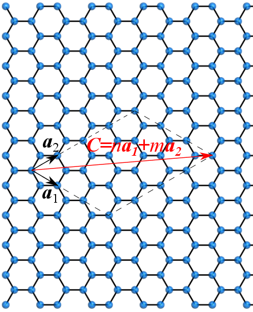
where $\hat{\boldsymbol{x}}$ and $\hat{\boldsymbol{y}}$ are two orthonormal vectors. The former is aligned along the armchair direction (Fig. 1). $\theta$ is the maximum stretch angle relative to the armchair direction and defined as

$$\begin{array}[]{lll}\theta\!\!\!&:=&\!\!\!\arccos{(\boldsymbol{Y}_{1}\cdot\hat{\boldsymbol{x}})}~{}.\end{array}$$ (47)

Figure 1: Orthonormal vectors characterizing the undeformed graphene lattice.

Then, the membrane strain energy density, per unit area of the initial configuration, can be decomposed into pure dilatation $W_{\text{m}}^{\mathrm{dil}}$ and deviatoric $W_{\text{m}}^{\mathrm{dev}}$ parts as

$$\begin{array}[]{l}W_{\text{m}}(\mathcal{J}_{1},\mathcal{J}_{2},\mathcal{J}_{3})=W_{\text{m}}^{\mathrm{dil}}(\mathcal{J}_{1})+W_{\text{m}}^{\mathrm{dev}}(\mathcal{J}_{2},\,\mathcal{J}_{3};\mathcal{J}_{1})~{}.\end{array}$$ (48)

The dilatation and deviatoric parts of the strain energy density are

$$\begin{array}[]{lll}W_{\text{m}}^{\mathrm{dil}}\!\!\!&:=&\!\!\!\varepsilon\big{[}1-(1+\hat{\alpha}\,\epsilon_{\mathrm{a}})\,\exp(-\hat{\alpha}\,\epsilon_{\mathrm{a}})\big{]}~{},\\[5.69054pt] W_{\text{m}}^{\mathrm{dev}}\!\!\!&:=&\!\!\!2\,\mu(\epsilon_{\mathrm{a}})\,\mathcal{J}_{2}+\eta(\epsilon_{\mathrm{a}})\,\mathcal{J}_{3}~{},\end{array}$$ (49)

where $\mu$ and $\eta$ are defined as

$$\begin{array}[]{lll}\mu(\epsilon_{\mathrm{a}})\!\!\!&:=&\!\!\!\mu_{0}-\mu_{1}\,e^{\hat{\beta}\,\epsilon_{\mathrm{a}}}~{},\\[5.69054pt] \eta(\epsilon_{\mathrm{a}})\!\!\!&:=&\!\!\!\eta_{0}-\eta_{1}\,\epsilon_{\mathrm{a}}^{2}~{}.\end{array}$$ (50)

The membrane model is thus characterized by the seven material constants $\varepsilon$, $\hat{\alpha}$, $\mu_{0}$, $\mu_{1}$, $\hat{\beta}$, $\eta_{0}$, and $\eta_{1}$ . They are given in Tab. 1. In that table, LDA and GGA are abbreviations for local density approximation and generalized gradient approximation. These are two approximations used in DFT simulations in order to compute the material constants. Using the relations given in the previous section, the contra-variant component of the Kirchhoff stress tensor for the cases of distinct and repeated eigenvalues are

$$\begin{array}[]{lll}\tau^{\alpha\beta}_{\text{m}}\!\!\!&=&\!\!\!\big{[}\varepsilon\,\hat{\alpha}^{2}\,\epsilon_{\mathrm{a}}\,e^{-\hat{\alpha}\,\epsilon_{\mathrm{a}}}-2\,(\eta_{1}\,\epsilon_{\mathrm{a}}\,\mathcal{J}_{3}+\mu_{1}\,\hat{\beta}\,\mathcal{J}_{2}\,e^{\hat{\beta}\,\epsilon_{\mathrm{a}}})\big{]}\,a^{\alpha\beta}+2\,\mu\,\ln\lambda\,\chi^{\alpha\,\beta}+\displaystyle\frac{1}{4}\,\eta\,\mu^{\alpha\beta},~{}\text{for}~{}\lambda_{1}\neq\lambda_{2}~{},\end{array}$$ (51)

and

$$\begin{array}[]{lll}\tau^{\alpha\beta}_{\text{m}}\!\!\!&=&\!\!\!\big{[}\varepsilon\,\hat{\alpha}^{2}\,\epsilon_{\mathrm{a}}\,e^{-\hat{\alpha}\,\epsilon_{\mathrm{a}}}\big{]}\,a^{\alpha\beta},~{}\text{for}~{}\lambda_{1}=\lambda_{2}~{},\end{array}$$ (52)

where $\mu^{\alpha\beta}$ and $\chi^{\alpha\,\beta}$ are defined as

$$\begin{array}[]{lll}\mu^{\alpha\beta}\!\!\!&:=&\!\!\!\displaystyle\sum\limits_{i,j=1,2}{f_{ij}\,P_{i}^{\alpha\gamma}\,T^{(0)}_{\gamma\delta}\,P_{j}^{\delta\beta}}~{},\end{array}$$ (53)

$$\begin{array}[]{lll}\chi^{\alpha\beta}\!\!\!&:=&\!\!\!\displaystyle\frac{1}{\lambda_{1}^{2}}\,P_{1}^{\alpha\beta}\,-\frac{1}{\lambda_{2}^{2}}\,P_{2}^{\alpha\beta}~{},\end{array}$$ (54)

and $f_{ij}$ is defined as

$$\begin{array}[]{lll}f_{ij}\!\!\!&:=&\!\!\!\left\{\begin{array}[]{l}\displaystyle\frac{1}{2\,\lambda_{i}^{2}}~{},\quad$if $i=j~{},\\[11.38109pt] \displaystyle\frac{\ln\lambda_{i}-\ln\lambda_{j}}{\lambda_{i}^{2}-\lambda_{j}^{2}}~{},\quad$if $i\neq j~{}.\end{array}\right.\end{array}$$ (55)

$T^{(0)}_{\gamma\delta}$ and the elasticity tensors related to Eqs. (51) and (52) are given in Appendix B.
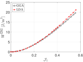
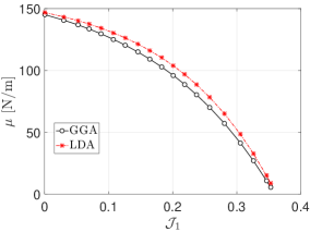
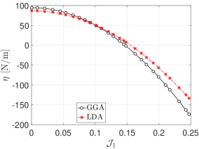
The variation of $W_{\text{m}}^{\mathrm{dil}}$, $\mu$ and $\eta$ with $\mathcal{J}_{1}$ are presented in Fig. 2. The elastic modulus of the current model is compared with reference data in Tab. 2. The elastic modulus of the current model is closer to existing experiments and ab-initio results than the exponential Cauchy-Born rule.

	$\hat{\alpha}$	$\varepsilon~{}[\textnormal{N/m}]$	$\mu_{0}~{}[\textnormal{N/m}]$	$\mu_{1}~{}[\textnormal{N/m}]$	$\hat{\beta}$	$\eta_{0}~{}[\textnormal{N/m}]$	$\eta_{1}~{}[\textnormal{N/m}]$
GGA	1.53	93.84	172.18	27.03	5.16	94.65	4393.26
LDA	1.38	116.43	164.17	17.31	6.22	86.93.1	3611.53.1

Table 1: Membrane behavior: Material constants of graphene (Kumar and Parks,, 2014).

	Elastic modulus E [${\color[rgb]{0,0,0}\mathrm{N/m}}$]
Exp. Cauchy-Born with FGBP (Arroyo and Belytschko, 2004a, )	236
Exp. Cauchy-Born with SGBP (Arroyo and Belytschko, 2004a, )	243
MM3 (Gupta and Batra,, 2010)	340
Current model with GGA (Kumar and Parks,, 2014)	349
Current model with LDA (Kumar and Parks,, 2014)	354
Ab initio (Kudin et al.,, 2001)	345
Experimental (Lee et al.,, 2008)	340

Table 2: Membrane behavior: Comparison of the elastic modulus for various methods. FGBP = first generation Brenner potential; SGBP = second generation Brenner potential; LDA = local density approximation; GGA = generalized gradient approximation.

(a)

(b)

(c)

Figure 2: Membrane behavior: Variation of (2(a)) dilatation Energy $W_{\text{m}}^{\mathrm{dil}}$, (2(b)) shear modulus $\mu$ and (2(c)) anisotropic part $\eta$ with $\mathcal{J}_{1}$ for the model of Kumar and Parks, (2014).

3.2 Bending energy

In this section, the membrane model of Kumar and Parks, (2014) is extended to a shell model by including a bending strain energy. In the current work, the uniaxial bending model of Lu et al., (2009) is extended to tensorial form using the tensorial invariants introduced in Sec. 2. Lu et al., (2009) show that the bending behavior of graphene is linear up to the curvature 1 $\mathrm{nm}^{-1}$ and the material response is isotropic below this limit. They used FGBP and SGBP to determine the material parameter of their bending model. In the former, only the bond angle is included and in the latter the dihedral angle is included in the potential. Lu et al., (2009) report the bending moduli 0.133 and 0.225 nN$\cdot$nm obtained from FGBP and SGBP (Brenner,, 1990; Brenner et al.,, 2002). The latter is much closer to existing ab-initio energy calcluations, which determine the bending modulus at 0.238 nN$\cdot$nm (Kudin et al.,, 2001). These bending parameters are summarized in Tab. 3. In all the following simulations the bending modulus is taken as 0.238 nN$\cdot$nm unless otherwise mentioned. The bending stiffness of graphene is not due to its thickness. The main source of the bending stiffness of graphene is the changing of bond angles and dihedral angles. The model of Canham, (1970) is a good candidate for modeling the bending of graphene. The Canham bending strain energy density per unit current area can be written as

$$\begin{array}[]{lll}w_{\mathrm{b}}=\displaystyle\frac{c}{2}\left(\kappa_{1}^{2}+\kappa_{2}^{2}\right)~{},\end{array}$$ (56)

where $c$ is a material constant. Since $\kappa_{1}$ and $\kappa_{2}$ depend on the in-plane stretch, model (56) introduces coupling between membrane and bending deformation. The bending strain energy per unit of current area can be transformed to the reference area as

$$\begin{array}[]{lll}\displaystyle W_{\mathrm{b}}=\displaystyle J\,\frac{c}{2}\left(\kappa_{1}^{2}+\kappa_{2}^{2}\right)~{}.\end{array}$$ (57)

The final form of the Kirchhoff stress and bending moment tensors due to bending are

$$\begin{array}[]{lll}\displaystyle\tau^{\alpha\beta}_{\mathrm{b}}\!\!\!&=&\!\!\!\displaystyle J\,\left[c\,(2H^{2}+\kappa)a^{\alpha\beta}-4c\,H\,b^{\alpha\beta}\right]~{},\end{array}$$ (58)

and

$$\begin{array}[]{lll}M^{\alpha\beta}_{0}=c\,J\,b^{\alpha\beta}~{}.\end{array}$$ (59)

The elasticity tensors for bending can be found in Sauer and Duong, (2017). As seen from (59), the Canham model leads to a simple linear relationship between curvature and bending moment. The coefficient of proportionality, $c$, corresponds to the bending stiffness. An advantage of the Canham model is that it does not require the notion of a thickness. An alternative approach is to use 3D elasticity and apply thickness integration as is considered in the formulation of Delfani and Shodja, (2016).

	FGBP	SGBP	QM
c [nN$\cdot$nm]	0.133	0.225	0.238

Table 3: Bending behavior: Bending stiffness according to various atomistic and quantum models (Lu et al.,, 2009; Kudin et al.,, 2001).

4 Finite element formulation

The presented graphene material model is implemented within the isogeometric rotation-free shell formulation of Duong et al., (2017), which is briefly summarized here. This section starts with the equilibrium equation and the corresponding discretization approximations. Then, the weak form is presented. Finally, the stiffness matrices are obtained based on standard linearization.

4.1 Equilibrium equation

The equilibrium equation for a Kirchhoff-Love shell can be written as

$$\begin{array}[]{l}\boldsymbol{T}_{;\alpha}^{\alpha}+\boldsymbol{f}=\rho\,\dot{\boldsymbol{v}}~{}~{}~{}\forall~{}\boldsymbol{x}~{}\in~{}\mathcal{B}~{},\end{array}$$ (60)

where “;” is the co-variant derivative, $\boldsymbol{T}^{\alpha}=\mbox{\boldmath$\sigma$}^{\mathrm{T}}\cdot\boldsymbol{a}^{\alpha}$ , and $\boldsymbol{f}$ and $\dot{\boldsymbol{v}}$ are body force and acceleration vectors. $\boldsymbol{f}$ and the boundary conditions can be defined as

$$\begin{array}[]{llll}\boldsymbol{f}&:=&f^{\alpha}\,\boldsymbol{a}_{\alpha}+p\,\boldsymbol{n}{}{}&\forall~{}\boldsymbol{x}~{}\in~{}~{}\mathcal{B}~{},\\[2.84526pt] \boldsymbol{u}&:=&\bar{\boldsymbol{u}}{}{}&\forall~{}\boldsymbol{x}~{}\in~{}\partial\mathcal{B}_{u}~{},\\[2.84526pt] \boldsymbol{n}&:=&\bar{\boldsymbol{n}}{}{}&\forall~{}\boldsymbol{x}~{}\in~{}\partial\mathcal{B}_{n}~{},\\[2.84526pt] \boldsymbol{t}&:=&\bar{\boldsymbol{t}}{}{}&\forall~{}\boldsymbol{x}~{}\in~{}\partial\mathcal{B}_{t}~{},\\[2.84526pt] m_{\tau}&:=&\bar{m}_{\tau}{}{}&\forall~{}\boldsymbol{x}~{}\in~{}\partial\mathcal{B}_{\tau}~{},\end{array}$$ (61)

where $\bar{\boldsymbol{u}}$ and $\bar{\boldsymbol{n}}$ are prescribed position and normal unit vector at the Dirichlet boundary, and $\bar{\boldsymbol{t}}$ and $\bar{m}_{\tau}$ are tractions and the bending moments at the Neumann boundary.

4.2 Discretization

The continua in current, $\mathcal{B}$ , and reference, $\mathcal{B}_{0}$ , configuration can be discretized with NURBS shape functions and control points as

$$\begin{array}[]{l}\boldsymbol{X}=\mathbf{N}\,\mathbf{X}_{n_{e}}~{};~{}\boldsymbol{x}=\mathbf{N}\,\mathbf{x}_{n_{e}}~{},\end{array}$$ (62)

where $\mathbf{N}$ and $n_{e}$ are the NURBS shape function matrix and the number of control points per element. Using the same shape functions, the following relations can be obtained

$$\begin{array}[]{lll}\delta\boldsymbol{x}\!\!\!&=&\!\!\!\mathbf{N}\,\delta\mathbf{x}_{n_{e}}~{},\\ \boldsymbol{a}_{\alpha}\!\!\!&=&\!\!\!\mathbf{N}_{,\alpha}\,\mathbf{x}_{n_{e}}~{},\\ \delta\boldsymbol{a}_{\alpha}\!\!\!&=&\!\!\!\mathbf{N}_{,\alpha}\,\delta\mathbf{x}_{n_{e}}~{},\\ \boldsymbol{a}_{\alpha,\beta}\!\!\!&=&\!\!\!\mathbf{N}_{,\alpha\beta}\,\mathbf{x}_{n_{e}}~{},\\ \boldsymbol{a}_{\alpha;\beta}\!\!\!&=&\!\!\!\tilde{\mathbf{N}}_{;\alpha\beta}\,\mathbf{x}_{n_{e}}~{},\\ \end{array}$$ (63)

where “,” is the parametric derivative and $\mathbf{N}$ , $\mathbf{N}_{,\alpha}$ , $\mathbf{N}_{,\alpha\beta}$ , and $\tilde{\mathbf{N}}_{;\alpha\beta}$ are defined as

$$\begin{array}[]{lll}\mathbf{N}\!\!\!&:=&\!\!\![N_{1}\,\boldsymbol{1},N_{2}\,\boldsymbol{1},\ldots,N_{n_{e}}\,\boldsymbol{1}]~{},\\[2.84526pt] \mathbf{N}_{,\alpha}\!\!\!&:=&\!\!\![N_{1,\alpha}\,\boldsymbol{1},N_{2,\alpha}\,\boldsymbol{1},\ldots,N_{n_{e},\alpha}\,\boldsymbol{1}]~{},\\[2.84526pt] \mathbf{N}_{,\alpha\beta}\!\!\!&:=&\!\!\![N_{1,\alpha\beta}\,\boldsymbol{1},N_{2,\alpha\beta}\,\boldsymbol{1},\ldots,N_{n_{e},\alpha\beta}\,\boldsymbol{1}]~{},\\[2.84526pt] \tilde{\mathbf{N}}_{;\alpha\beta}\!\!\!&:=&\!\!\!\mathbf{N}_{,\alpha\beta}-\Gamma_{\alpha\beta}^{\gamma}\,\mathbf{N}_{,\gamma}~{},\end{array}$$ (64)

where $N_{i}$ are NURBS shape functions. Using approximations (Eqs. (62) and (LABEL:e:dis_surface_object)), the weak form can be written as

$$\begin{array}[]{l}\displaystyle\sum\limits_{e=1}^{n_{\text{el}}}{(G_{\text{in}}^{e}+G_{\text{int}}^{e}+G_{\text{c}}^{e}-G_{\text{ext}}^{e})}=0~{},\forall~{}\delta\mathbf{x}_{e}\in\mathcal{B}~{},\end{array}$$ (65)

where $n_{\text{el}}$ is the number of elements. $G_{\mathrm{c}}^{e}$ is related to contact and is discussed in Appendix D.2. $G_{\text{in}}^{e}$, $G_{\text{int}}^{e}$, and $G_{\text{ext}}^{e}$ are inertial, internal and external parts and are defined as

$$\begin{array}[]{llll}G_{\text{in}}^{e}:=\delta\mathbf{x}_{e}^{\text{T}}\,\mathbf{f}_{\text{in}}^{e}~{};~{}~{}~{}\text{with}~{}~{}\mathbf{f}_{\text{in}}^{e}=\displaystyle\int\limits_{\mathcal{B}_{0}^{e}}{\mathbf{N}^{\text{T}}\,\rho\,\dot{\boldsymbol{v}}~{}\mathrm{d}A}~{},\end{array}$$ (66)

$$\begin{array}[]{lll}G_{\text{int}}^{e}:=\delta\mathbf{x}_{e}^{\text{T}}\,(\mathbf{f}_{\text{int}\tau}^{e}+\mathbf{f}_{\text{int}M}^{e})~{};~{}~{}\text{with}~{}~{}\mathbf{f}_{\text{int}\tau}^{e}=\displaystyle\int\limits_{\mathcal{B}_{0}^{e}}{\tau^{\alpha\beta}\,\mathbf{N}_{,\alpha}^{\text{T}}\,\boldsymbol{a}_{\beta}~{}\mathrm{d}A}~{};~{}\mathbf{f}_{\text{int}M}^{e}=\displaystyle\int\limits_{\mathcal{B}_{0}^{e}}{M_{0}^{\alpha\beta}\,\tilde{\mathbf{N}}_{;\alpha\beta}^{\text{T}}\,\boldsymbol{n}~{}\mathrm{d}A}~{},\end{array}$$ (67)

$$\begin{array}[]{lll}G_{\text{ext}}^{e}\!\!\!&:=&\!\!\!\delta\mathbf{x}_{e}^{\text{T}}\,\left(\mathbf{f}_{\text{ext}0}^{e}+\mathbf{f}_{\text{ext}p}^{e}+\mathbf{f}_{\text{ext}t}^{e}+\mathbf{f}_{\text{ext}m}^{e}\right)~{}.\end{array}$$ (68)

The terms in Eq. (68) are

$$\begin{array}[]{lll}\mathbf{f}_{\text{ext}0}^{e}\!\!\!&=&\!\!\!\displaystyle\int\limits_{\mathcal{B}_{0}^{e}}{\mathbf{N}^{\text{T}}\,\boldsymbol{f}_{0}~{}\mathrm{d}A}~{},\\[8.53581pt] \mathbf{f}_{\text{ext}p}^{e}\!\!\!&=&\!\!\!\displaystyle\int\limits_{\mathcal{B}^{e}}{\mathbf{N}^{\text{T}}\,p\,\boldsymbol{n}~{}\mathrm{d}a}~{},\\[8.53581pt] \mathbf{f}_{\text{ext}t}^{e}\!\!\!&=&\!\!\!\displaystyle\int\limits_{\partial_{t}\mathcal{B}^{e}}{\mathbf{N}^{\text{T}}\,\boldsymbol{t}~{}\mathrm{d}s}~{},\\[8.53581pt] \mathbf{f}_{\text{ext}m}^{e}\!\!\!&=&\!\!\!\displaystyle-\int\limits_{\partial_{m}\mathcal{B}^{e}}{\mathbf{N}_{,\alpha}^{\text{T}}\,\nu^{\alpha}\,m_{\tau}\,\boldsymbol{n}~{}\mathrm{d}s}~{},\end{array}$$ (69)

where along $\partial_{m}\mathcal{B}$ bending Neumann BCs are applied. $\nu^{\alpha}$ are the contra-variant components of the normal vector on the boundary $\partial\mathcal{B}$.

4.3 Stiffness matrix

The stiffness matrix appearing in the linearization of the discretized weak form, can be written as

$$\begin{array}[]{lll}\mathbf{k}^{e}\!\!\!&=&\!\!\!\mathbf{k}_{\tau\tau}^{e}+\mathbf{k}_{\tau M}^{e}+\mathbf{k}_{M\tau}^{e}+\mathbf{k}_{MM}^{e}+\mathbf{k}_{\tau}^{e}+\mathbf{k}_{M}^{e}+\mathbf{k}_{\text{extp}}^{e}+\mathbf{k}_{\text{extm}}^{\text{e}}+\mathbf{k}_{c}^{e}~{},\end{array}$$ (70)

where the material stiffness matrices are defined by

$$\begin{array}[]{lll}\mathbf{k}_{\tau\tau}^{e}\!\!\!&:=&\!\!\!\displaystyle\int\limits_{\mathcal{B}_{0}^{e}}{{c}^{\alpha\beta\gamma\delta}\,\mathbf{N}_{,\alpha}^{\text{T}}\,(\boldsymbol{a}_{\beta}\otimes\boldsymbol{a}_{\gamma})\,\mathbf{N}_{,\delta}~{}\mathrm{d}A}~{},\\[22.76219pt] \mathbf{k}_{\tau M}^{e}\!\!\!&:=&\!\!\!\displaystyle\int\limits_{\mathcal{B}_{0}^{e}}{{d}^{\alpha\beta\gamma\delta}\,\mathbf{N}_{,\alpha}^{\text{T}}\,(\boldsymbol{a}_{\beta}\otimes\boldsymbol{n})\,\tilde{\mathbf{N}}_{;\gamma\delta}~{}\mathrm{d}A}~{},\\[22.76219pt] \mathbf{k}_{M\tau}^{e}\!\!\!&:=&\!\!\!\displaystyle\int\limits_{\mathcal{B}_{0}^{e}}{{e}^{\alpha\beta\gamma\delta}\,\tilde{\mathbf{N}}_{;\alpha\beta}^{\text{T}}\,(\boldsymbol{n}\otimes\boldsymbol{a}_{\gamma})\,\mathbf{N}_{,\delta}~{}\mathrm{d}A}~{},\\[22.76219pt] \mathbf{k}_{MM}^{e}\!\!\!&:=&\!\!\!\displaystyle\int\limits_{\mathcal{B}_{0}^{e}}{{f}^{\alpha\beta\gamma\delta}\,\tilde{\mathbf{N}}_{;\alpha\beta}^{\text{T}}\,(\boldsymbol{n}\otimes\boldsymbol{n})\,\tilde{\mathbf{N}}_{;\gamma\delta}~{}\mathrm{d}A}~{},\end{array}$$ (71)

where the elasticity tensors are given in Appendix B and Sauer and Duong, (2017). Furthermore, the geometrical stiffness matrices are defined as

$$\begin{array}[]{lll}\mathbf{k}_{\tau}^{e}\!\!\!&:=&\!\!\!\displaystyle\int\limits_{\mathcal{B}_{0}^{e}}{\mathbf{N}_{,\alpha}^{\text{T}}\,\tau^{\alpha\beta}\,\mathbf{N}_{,\beta}~{}\mathrm{d}A}~{},\end{array}$$ (72)

$$\begin{array}[]{lll}\mathbf{k}_{M}^{e}\!\!\!&:=&\!\!\!\displaystyle\mathbf{k}_{M1}^{e}+\mathbf{k}_{M2}^{e}+(\mathbf{k}_{M2}^{e})^{\text{T}}~{},\end{array}$$ (73)

with

$$\begin{array}[]{lll}\mathbf{k}_{M1}^{e}\!\!\!&:=&\!\!\!\displaystyle-\int\limits_{\mathcal{B}_{0}^{e}}{b_{\alpha\beta}\,M^{\alpha\beta}_{0}\,a^{\gamma\delta}\,\mathbf{N}_{,\gamma}^{\text{T}}\,(\boldsymbol{n}\otimes\boldsymbol{n})\,\mathbf{N}_{,\delta}~{}\mathrm{d}A}~{},\\[22.76219pt] \mathbf{k}_{M2}^{e}\!\!\!&:=&\!\!\!\displaystyle-\int\limits_{\mathcal{B}_{0}^{e}}{M^{\alpha\beta}_{0}\,\mathbf{N}_{,\gamma}^{\text{T}}\,(\boldsymbol{n}\otimes\,a^{\gamma})\,\tilde{\mathbf{N}}_{;\alpha\,\beta}~{}\mathrm{d}A}~{}.\end{array}$$ (74)

The external tangent matrices $\mathbf{k}_{\text{extp}}^{e}$ and $\mathbf{k}_{\text{extm}}^{e}$ can be found in Sauer et al., (2014) and Duong et al., (2017), and the contact stiffness matrix $\mathbf{k}_{c}^{e}~{}$ is given in Appendix D.2.

5 Elementary model behavior

In this section, the elementary behavior of the model under some simple deformation states is investigated. Pure dilatation, uniaxial stretch, pure shear and pure bending are considered as test cases, and the FE implementation is verified by analytical solutions.

Figure 3: Elementary membrane deformations: (a) Pure dilatation; (b) uniaxial stretch; (c) pure shear; (d) considered FE mesh; linear Lagrangian elements are used and the nodes are indicated by $\bullet$. Angle $\theta$ denotes the orientation of the graphene lattice with respect to the direction of larger stretch $\lambda_{1}$ , and $\lambda_{0}>1$ is gradually increased.

5.1 Pure dilatation

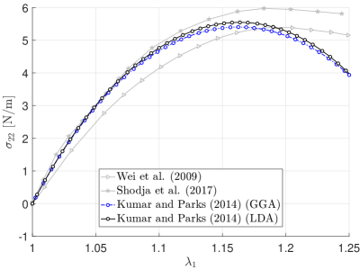
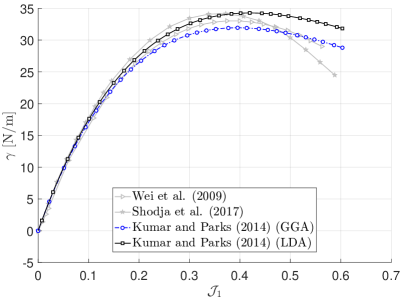
The numerical model consists of a square sheet stretched uniformly in two perpendicular directions. The boundary conditions and the lattice orientation are shown in Fig. 3a. The surface tension $\gamma:=\frac{1}{2}\mathrm{tr}\,(\mbox{\boldmath$\sigma$})$ is obtained with the LDA and the GGA parameters and the results are compared in Fig. 4. The current continuum model is compared with quantum results from the literature. The difference of LDA and GGA results is small for infinitesimal strains. But, the response is different for finite strains, where LDA shows a stiffer response. It should be noted that the material is unstable after the maximum value of the surface tension has been reached. The shear modulus is zero at this point and become negative afterwards. Displacement control is needed to go beyond that point.

Figure 4: Pure dilatation: Surface tension. The current continuum model is based on the quantum mechanical results of Kumar and Parks, (2014). Other quantum mechanical results are available in Wei et al., (2009) and Shodja et al., (2017).

5.2 Uniaxial stretch

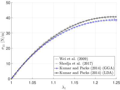
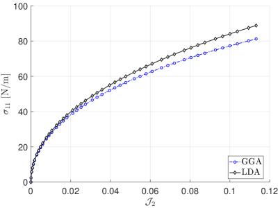
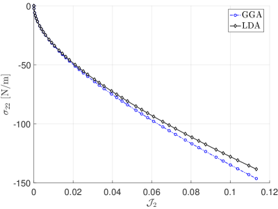
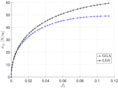
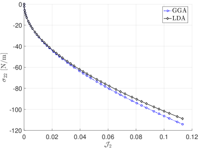
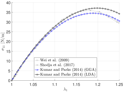
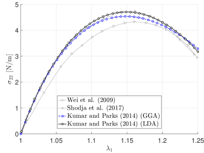
Uniaxial stretching is considered along different directions, i.e. different chiralities. The model is stretched in one direction and restrained in the perpendicular direction (Fig. 3b). In order to assess the FE solution, the Cartesian stress components $\sigma_{11}$ and $\sigma_{22}$ are examined. They are the normal stress components in the direction of the stretch and perpendicular to it. They are obtained analytically in Appendix C. The results of stretching the model in the armchair and the zigzag directions are presented in Figs. 5 and 6. The current continuum model is compared with quantum results from the literature. Like for dilatational loading, a material instability occurs after the maximum stress has been reached and the elasticity tensor loses its ellipticity at this point.
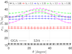
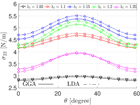
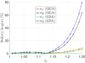
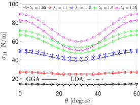
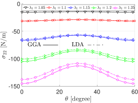
Next, the model is stretched in different directions, relative to the armchair direction, and the stress variation is examined for a set of stretch ratios in Fig. 7. As can be expected, the material response is periodic by $\pi/3$. Finally, the standard deviation and average of the stresses in one period is calculated for the different stretch ratios. The average and standard deviation can be calculated as

$$\begin{array}[]{lll}\displaystyle\text{Avg}(\sigma_{ij})\!\!\!&=&\!\!\!\displaystyle\langle\sigma_{ij}\rangle~{}=~{}\frac{3}{\pi}\int_{0}^{\pi/3}{\sigma_{ij}~{}{\color[rgb]{0,0,0}\mathrm{d}\theta~{},}}\end{array}$$ (75)

$$\begin{array}[]{lll}\displaystyle\text{Std}(\sigma_{ij})\!\!\!&=&\!\!\!\displaystyle\int_{0}^{\pi/3}{\sqrt{\frac{3}{\pi}(\sigma_{ij}-\langle\sigma_{ij}\rangle)^{2}}~{}\mathrm{d}\theta}~{}.\end{array}$$ (76)

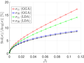
The standard deviation is normalized by the average stress and shown versus $\lambda_{1}$  in Fig. 7(c). The graph can be interpreted as the error caused by assuming isotropy. This error can reach up to 80% of the average response. So, an anisotropic model is necessary to capture the material behavior for finite deformations.

(a)

(b)

Figure 5: Uniaxial stretch in the armchair direction: (6(a)) Stress in the stretched direction, $\sigma_{11}$; (6(b)) stress in the perpendicular direction, $\sigma_{22}$. The current continuum model is based on the quantum mechanical results of Kumar and Parks, (2014). Other quantum mechanical results are available in Wei et al., (2009) and Shodja et al., (2017).

(a)

(b)

Figure 6: Uniaxial stretch in the zigzag direction: (6(a)) Stress in the stretched direction, $\sigma_{11}$; (6(b)) stress in the perpendicular direction, $\sigma_{22}$. The current continuum model is based on the quantum mechanical results of Kumar and Parks, (2014). Other quantum mechanical results are available in Wei et al., (2009) and Shodja et al., (2017).

(a)

(b)

(c)

Figure 7: Uniaxial stretch: Dependence of the stress components on stretch $\lambda_{1}$ and angle $\theta$, (7(a)) $\sigma_{11}$; (7(b)) $\sigma_{22}$. (7(c)) Dependence of the standard deviation of the stress on stretch $\lambda_{1}$.

5.3 Pure shear

Pure shear is considered in different directions, i.e. different chiralities. Therefore, the specimen is pulled in one direction and compressed in the perpendicular direction by $\lambda_{1}=\lambda_{0}>1$ and $\lambda_{2}=1/\lambda_{0}$ such that $J=\lambda_{1}\,\lambda_{2}=1$ (Fig. 3c). The Cartesian stress components $\sigma_{11}$ and $\sigma_{22}$ are introduced and analytically derived in Appendix  C. The stress variation versus $\mathcal{J}_{2}$, in the pull and compression direction, for the armchair and zigzag direction, are shown in Figs. 8 and 9.
Next, the loading is applied in different directions, relative to the armchair direction, and stress variation is demonstrated for a set of stretch ratios and GGA and LDA parameters in Fig. 10. The graphes show the similar periodic behavior as noted in the previous section. Finally, the standard deviation and average of the stresses in one period are calculated for the different stretch ratios. The standard deviation is normalized by the average stress and it is shown versus $\mathcal{J}_{2}$ in Fig. 10(c). Like for uniaxial stretch, the graph can be interpreted as the error caused by assuming isotropy. As shown, this error can reach up to 17 percent. The anisotropic behavior is increasing fast even for low values of $\mathcal{J}_{2}$.

(a)

(b)

Figure 8: Pure shear with pull in the armchair and compression in the zigzag direction ($\theta=0$ in Fig. 3): (8(a)) Stress in the pull direction, $\sigma_{11}$; (8(b)) stress in the compression direction, $\sigma_{22}$.

(a)

(b)

Figure 9: Pure shear with pull in the zigzag and compression in the armchair direction ($\theta=\pi/6$ in Fig. 3): (9(a)) Stress in the pull direction, $\sigma_{11}$; (9(b)) stress in the compression direction, $\sigma_{22}$.

(a)

(b)

(c)

Figure 10: Pure shear: Dependence of the stress components on stretch $\lambda_{1}$ and angle $\theta$, (10(a)) $\sigma_{11}$; (10(b)) $\sigma_{22}$. (10(c)) Dependence of the standard deviation of the stress on $\mathcal{J}_{2}$.

5.4 Pure bending

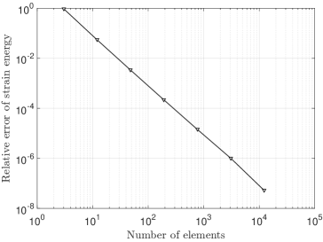
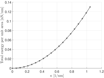
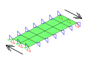
In this section, the bending formulation is validated by considering pure bending. The boundary conditions are shown in Fig. 11(a). The specimen’s width is restrained and it is stress free in the longitudinal direction. The details of the analytical solution for pure bending can be found in Sauer and Duong, (2017). The resultant force along the longitudinal direction, $N_{1}^{1}$ (see Eq. (43)), is zero for pure bending. $N_{1}^{1}=0$ is solved by the standard secant method to obtain the analytical solution. The final geometry is plotted in Fig. 11(b). The convergence of the total energy is obtained with mesh refinement (Fig. 12(a)). The bending strain energy per unit reference area is shown in Fig. 12(b). The relation between bending moment and curvature is linear.

(a)

(b)

Figure 11: Pure bending: (11(a)) boundary conditions (the green, blue and red triangles indicate restriction of displacement dofs in the longitudinal, lateral and perpendicular directions, respectively; the arrows indicate prescribed rotations); (11(b)) deformed geometry.

(a)

(b)

Figure 12: Pure bending: (12(a)) Error of strain energy relative to the finest mesh ($384\times 128$ quadratic NURBS elements); (12(b)) total energy per unit reference area.

6 Numerical examples

In the previous section, the proposed model is verified by standard tests. In the current section, several numerical benchmark examples are solved and compared with results from the literature. Considered are five examples: indentation and peeling of graphene, and torsion, bending and uniaxial stretch of carbon nanotubes (CNTs).

6.1 Indentation of graphene

In order to compare the developed model with experimental results, an indentation problem is considered in this section. The experimental results are taken from a setup with multiple cavities. Relative position of these cavities can affect experimental measurements. In current numerical simulations, only one cavity is modeled and frictional effects are neglected. In the following subsections, first the specimen details, boundary conditions, and loading are discussed. Finally, a parameter study is conducted for the adhesion strength and indentor radius. Kumar and Parks, (2015) investigated the same problem using the Morse potential to model substrate interactions and ABAQUS (Abaqus,, 2016) in an explicit dynamic manner. In the current work, the Lennard-Jones potential and a quasi-static formulation is used.

6.1.1 Specimen details, boundary conditions and substrate adhesion

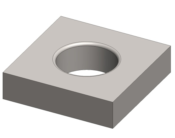
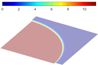
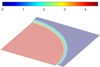
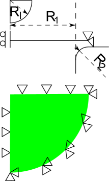
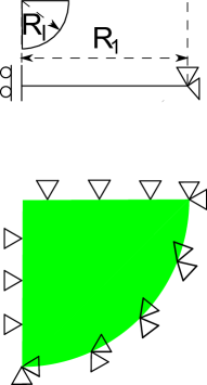
The problem setup consists of a sheet of graphene on a $\textnormal{SiO}_{2}$ substrate with a micro-cavity. The boundary conditions and geometry of the substrate are depicted in Fig. 13. For efficiency, only one quarter of the circular sheet is discretized. Thus, additional symmetry BCs have to be applied along the symmetry planes. In addition, the outer sheet boundary is fixed in all directions. The edge of the cavity is smoothed with a fillet radius of 50 nm. The adhesion plays an important role in the initial stress, stiffness and overall response of the sheet. A relaxation step is considered before the indentation loading. The adhesion between sheet and substrate is modeled via van der Waals (vdW) interaction (Appendix D). In the relaxation step, the adhesion parameter is increased from zero to its final value. At each step, a standard Newton Raphson iteration is utilized to determine equilibrium. The displacement and stress distribution of the relaxed geometry are shown in Fig. 14. This stress corresponds to a pre-stress within the graphene sheet that makes the structure stiffer.

(a)

(b)

(c)

Figure 13: Indentation setup: Outer boundary conditions and symmetry boundary conditions for (13(a)) adhesive substrate and (13(b)) substrate without adhesion; (13(c)) substrate geometry. $R_{I}$ is the indentor radius, $R_{1}$ the cavity radius and $R_{2}$ the fillet radius of the cavity.

(a)

(b)

Figure 14: Substrate adhesion of graphene: (14(a)) Displacement in the perpendicular direction to the graphene sheet after relaxation (in nm); (14(b)) $\text{tr}(\mbox{\boldmath$\sigma$})$ [N/m]. The adhesion strength $\Gamma$ and $\text{R}_{1}$ (see Fig. 13(a)) are set to 0.45 N/m and 500 nm, respectively. The maximum of tr($\sigma$) and the displacement are 4.95 N/m and 11.75 nm, respectively. In the simulation, all displacement dofs with a radial position greater than $R_{1}$ are fixed.

6.1.2 Indentation: Load step

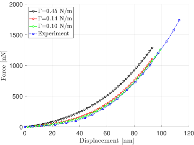
10000 quadratic isogeometric finite elements are used over a rectangular domain with the same number of elements in x and y directions. Before the indentation phase, a relaxation step is conducted. A wide range for adhesion strengths ($\Gamma=0.1\sim 0.45~{}\text{N/m}$) can be found in the literature discussed in Sec. 1. To study the influence of adhesion, the indentation simulation is conducted for a set of different $\Gamma$. The indented geometry is presented in Fig. 15. The indentor contact force is measured and compared with experimental results in Fig. 16(a). A higher adhesion strength results in a stiffer structure and a higher indentor reaction force.
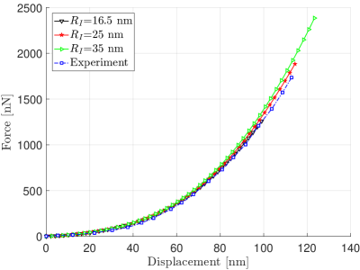
Next, to study the effect of the indentor size, a set of simulations are conducted for a series of indentors (Fig. 16(b)). They have the same force-displacement curve in the beginning of indentation. But, they have a different response for large indentation. In addition, a larger indentor has a larger reaction force.
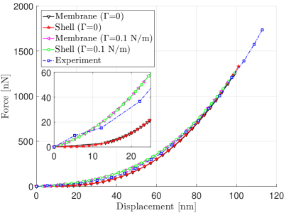
Finally, the problem is solved with zero bending stiffness (pure membrane model) and compared with the shell model for the substrate with and without adhesion. It is shown that the bending stiffness does not play an important role for the force-displacement curve (Fig. 17). In addition, in the cases without adhesion, it is assumed that the edge of the substrate cavity is not filleted and $R_{1}$ is selected to be consistent with the adhesive substrate setup (see Figs. 13(a) and 13(b)).

(a)

(b)

Figure 15: Graphene indentation: (15(a)) Indented profile (colored by tr$(\mbox{\boldmath$\sigma$})~{}[\text{N/m}]$); (15(b)) zoom of (15(a)). Adhesion parameter $\Gamma$, cavity radius $R_{1}$ and indentor radius $R_{I}$ are 0.45 N/m, 500 nm and 35 nm, respectively.

(a)

(b)

Figure 16: Graphene indentation, force-displacement curve of the indentor: (16(a)) Comparison between different adhesion parameters (for fixed $R_{1}=500$ nm and $R_{I}=16.5$ nm); (16(b)) comparison between different indentor radii (for fixed $\Gamma=0.1$ N/m and $R_{1}=500$ nm). The experimental results are taken from Kumar and Parks, (2015).

Figure 17: Graphene indentation: Comparison between membrane and shell models considering various values for $\Gamma$ (for fixed $R_{1}=500$ nm and $R_{I}=16.5$ nm). The experimental results are taken from Kumar and Parks, (2015).

6.2 Peeling of graphene

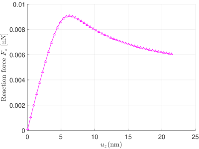
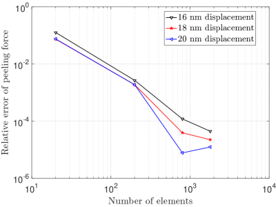
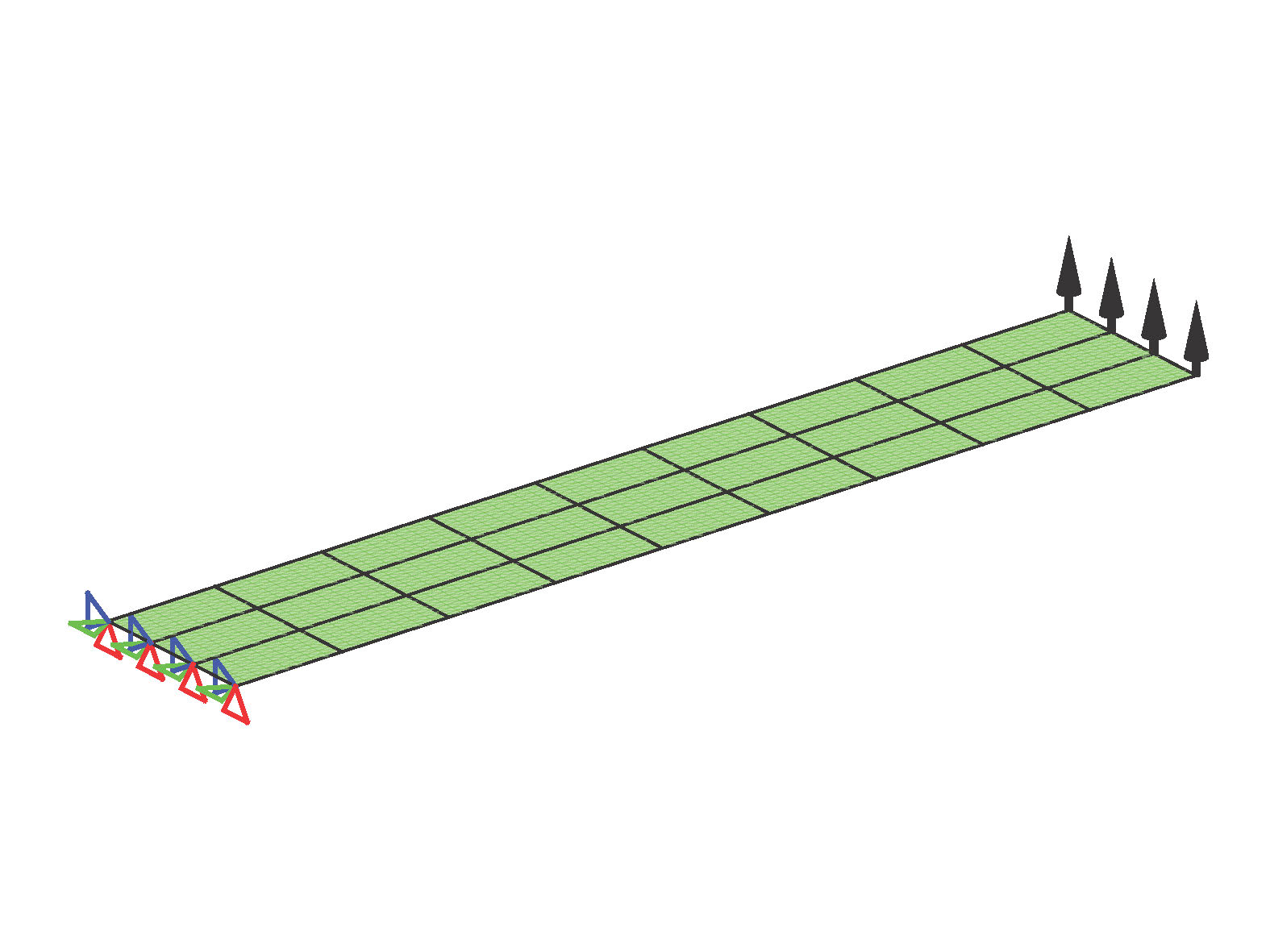
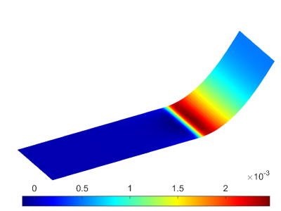
Peeling between graphene and an adhesive substrate is considered next. A rectangular graphene strip is considered that is initially positioned in equilibrium distance on a $\textnormal{SiO}_{2}$ substrate. The strip is restrained on one side and the other side is displaced in the perpendicular direction to the substrate ($u_{z}$) (Fig. 18(a)). The first 20 percent of the length of the strip are not absorbed to the substrate (the adhesion parameter is assumed to be zero in this area). Quadratic NURBS elements with the same element size in both directions are used in the simulation. The deformed geometry is plotted in Fig. 18(b). The convergence of the peeling force with mesh refinement is shown Fig. 19(b). Fig. 19(a) shows the peeling force against the peeling displacement. The peeling force exhibits an increasing and a decreasing part. They capture the elastic deformation and adhesive debonding of the strip, respectively.

(a)

(b)

Figure 18: Graphene peeling: (18(a)) The peeling setup (BC and loading). The size of the strip is $50\mathrm{nm}\times 10\mathrm{nm}$. (18(b)) The deformed geometry of the peeled strip colored by tr$(\mbox{\boldmath$\sigma$})~{}[\text{N/m}]$.

(a)

(b)

Figure 19: Graphene peeling: (19(a)) Peeling force vs. peeling displacement. (19(b)) Error of the peeling force for various peeling displacements relative to the finest mesh ($90\times 60$ quadratic NURBS elements). The LDA and FGBP parameter sets are used together with $\Gamma=0.14$ N/m.

6.3 Deformation of carbon nanotubes (CNTs)

In this section, the proposed shell model is applied to CNTs. First, the relaxation process is discussed. Then, the CNT behavior under torsional and bending loading is investigated. The results for torsion are compared and validated with atomistic results from the literature. In both loading scenarios, the buckling of shell walls is captured and the buckling load is accurately determined from the ratio of the membrane energy to the total energy. This energy ratio is determined from the strain energies introduced in Sec. 3.

6.3.1 Relaxation of CNTs

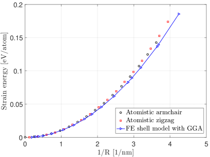
The CNT model needs to be relaxed in order to obtain a stress-free initial configuration (Favata et al.,, 2016). The internal energy is minimized in this relaxation process. During relaxation the CNT deforms radially while the length remains almost constant. The minimized strain energy per atom for CNTs with different chirality is compared with results from the literature in Fig. 20. The radius for CNT($n$,$m$) can be calculated as

$$\begin{array}[]{lll}R\!\!\!&=&\!\!\!\displaystyle\frac{\sqrt{3}a_{\text{cc}}}{2\pi}\sqrt{n^{2}+n\,m+m^{2}}~{},\end{array}$$ (77)

where the chirality parameters $n$ and $m$ indicate the number of the unit cells along the primary lattice vectors (Fig. 21). $a_{\text{cc}}=0.142$ nm is the equilibrium length of the carbon-carbon bond.

Figure 20: CNT relaxation: the strain energy per atom obtained after relaxation. $R$ denotes the radius of the CNT according to Eq. (77). For the finite element simulation different chiralities are used. The atomistic results are taken from Arroyo and Belytschko, 2004a .

Figure 21: CNT chirality: CNT($n$,0) and CNT($n$,$n$) indicate zigzag and armchair CNTs. $\boldsymbol{a}_{\alpha}$ are the primary lattice vectors.

6.3.2 Torsion of CNT

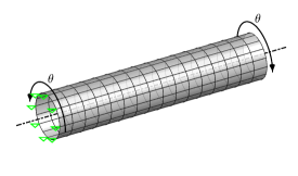
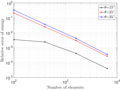
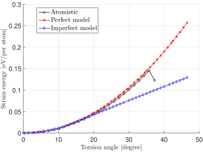
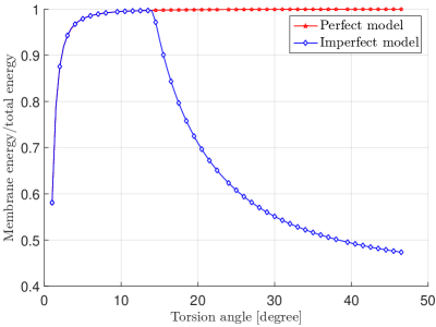
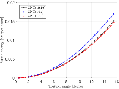
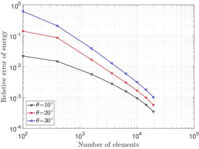
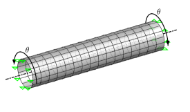
In this section, the behavior of an initially relaxed CNT under torsional loading is investigated. The loading can be conducted either by restraining the axial length of CNT (Fig. 22(a)) or letting the CNT deform in the axial direction (Fig. 22(b)). A torsion angle is applied to both ends of CNT, and the simulation is conducted with and without imperfection. The imperfection is applied as a torque in the middle of the CNT (Fig. 22(c)). The convergence is studied for the total energy (Fig. 23). The cross section of the model without imperfection remains cylindrical during torsion, i.e. it does not buckle, and the results converge faster in comparison to the model with imperfection. The strain energy per atom of CNT is plotted for the perfect and imperfect structures. The results from the presented model are compared to results from an atomistic simulation with a perfect crystal in Fig. 24(a). In the loading process, the CNT with the imperfection buckles, but the exact point of the instability is not easily found from the variation of the total energy. To estimate the instability point more accurately, the ratio of the membrane energy to the total energy is used. The sharp decreasing of energy ratio determines the buckling angle around ($\theta_{\mathrm{b}}=14^{\circ}$) (Fig. 24(b)). The strain energy is measured relative to the relaxed geometry. Next, a set of simulations is conducted for the different charities and the results are presented in Fig. 25. The deformed and sliced geometries are compared for different torsion angles (Fig. 26).

(a)

(b)

(c)

Figure 22: CNT twisting: BC for (22(a)) axially fixed case; (22(b)) axially free case; (22(c)) imperfection torque.

Figure 23: CNT twisting: Error of strain energy relative to the finest mesh ($100\times 100$ quadratic NURBS elements). CNT(12,6) with the length 6.74 nm is used for the axially fixed case (Fig. 22(a)).

(a)

(b)

Figure 24: CNT twisting: (24(a)) Strain energy per atom; (24(b)) ratio of the membrane energy to the total energy (measured relative to relaxed geometry). CNT(12,6) with the length 6.74 nm is used for the axially fixed case (Fig. 22(a)). The perfect and imperfect models are used for the simulation. The atomistic results are taken from Sun and Li, (2011).

Figure 25: CNT twisting: Strain energy per atom for different chiralities of CNTs with the length of 10 nm. CNTs are selected such that their radii are close to each other. The BC is set to the axially free case (Fig. 22(b)) and imperfection is applied to the model.

Figure 26: CNT twisting: Comparison of cross sections and tr($\sigma$) [N/m] at the torsion angles (a) $\theta=15^{\circ}$, (b) $\theta=25^{\circ}$, (c) $\theta=35^{\circ}$ and (d) $\theta=46.5^{\circ}$. CNT(12,6) with the length 6.74 nm is used. The BCs are applied according to the axially fixed case (Fig. 22(b)).

6.3.3 Bending of CNT

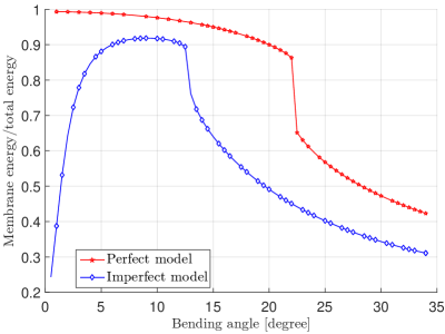
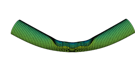
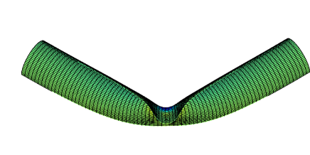
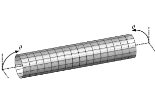
In this section, the behavior of a CNT under bending loading is investigated. CNT is bent by applying a bending angle equally at both ends (Fig. 27(a)). During bending, the end faces of the CNT are assumed to be rigid and remain planar, and the CNT can deform in axial direction in order to attain a state of pure bending loading. The strain energy convergence is studied with mesh refinement (Fig. 27(b)). The strain energy per atom is presented in Fig. 28(a) for perfect and imperfect structures and the buckling point is determined from the sharp variation in the ratio of the membrane energy to the total energy (Fig. 28(b)). It is shown that for the imperfect model, buckling occurs earlier. tr($\sigma$) is compared at different bending angles for the perfect and imperfect models (Fig. 29). Finally, the models are cut open along the axial direction to compare the buckled geometry of the perfect and imperfect CNTs (Fig. 30).

(a)

(b)

Figure 27: CNT bending: (27(a)) BC; (27(b)) Error of strain energy relative to the finest mesh ($200\times 200$ quadratic NURBS elements). CNT(10,10) with the length 10 nm and imperfection is used.

(a)

(b)

Figure 28: CNT bending: (28(a)) Comparison of strain energy per atom in perfect and imperfect cases; (28(b)) comparison of the ratio of the membrane energy to the total in perfect and imperfect cases. CNT(10,10) with the length 10 nm is used.

Figure 29: CNT bending: Comparison of tr($\sigma$) $[\text{N/m}]$ of the perfect and imperfect models for the bending angles (a) $\theta=10^{\circ}$, (b) $\theta=20^{\circ}$, (c) $\theta=30^{\circ}$ and (d) $\theta=34^{\circ}$. CNT(10,10) with the length 10 nm is used.

(a)

(b)

Figure 30: CNT bending: Cross sections of (30(a)) the perfect and (30(b)) the imperfect models ($\theta=34^{\circ}$). CNT(10,10) with the length 10 nm is used.

6.4 Stretch of chiral CNTs

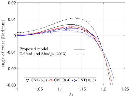
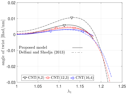
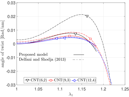
The deformation of chiral CNTs under axial loading is investigated here. The deformation includes a uniform extension and twisting along the axial direction of the CNT. The anisotropy of graphene is the source of this twisting. Three chiralities are selected, and the variation of the twist angle against the stretch is presented in Fig. 31. The results are compared with the results of Delfani and Shodja, (2013). There is very good agreement for large tube radii, but for small tube radii differences appear: Delfani and Shodja, (2013) find an initial twist at zero stretch that they argue appears from relaxing the initial energy of the original tube (that is a rolled graphene sheet with non-zero bending energy). The proposed model, on the other hand, relaxes the initial bending energy by a change of radius and does not predict an initial twist.

(a)

(b)

(c)

Figure 31: Stretch of chiral CNTs: Twist angle vs. stretch according to the proposed model and Delfani and Shodja, (2013) for various chirality angles. (31(a)) $\varphi=12.82^{\circ}$; (31(b)) $\varphi=13.90^{\circ}$ and (31(c)) $\varphi=19.11^{\circ}$. The chirality angle is defined as $\tan(\varphi):=\sqrt{3}\,m/(2n+m)$.

7 Conclusion

A new shell model is developed based on a new anisotropic membrane model and a new isogeometric shell formulation. The model is verified with standard biaxial, uniaxial and bending tests. It is used for the modeling of indentation and peeling of a graphene sheet, and the torsion, bending and stretching of a CNT. The new model is computationally more efficient than atomistic methods when the problem size reaches micrometer scale. In addition, the interatomic potentials presently used within the exponential Cauchy-Born rule (ECB) tend to underestimate the elastic modulus and bending stiffness obtained from quantum mechanics (QM). Also, molecular dynamics (MD) simulation have the same drawback as the ECB rule. The current model uses existing QM data to calibrate the material constants. The material response of the current model is therefore closer to existing ab-initio and experimental results. Thus the current model improves both accuracy and efficiency. Finally, the current model is fully nonlinear and can handle large deformations, buckling and postbuckling. The buckling points in torsional and bending loading are determined from the energy ratio, and the postbuckling behavior of CNTs is simulated.

Appendix A Tensorial derivative and curvilinear description of logarithmic strain

In this section, the derivative of eigenvalues and a formulation for the tensorial derivative of the logarithmic strain are given. Then, the logarithmic strain is described in curvilinear coordinates. The derivative of eigenvalues can be written as (Itskov,, 2015)

$$\begin{array}[]{l}\displaystyle\frac{\partial{\Lambda_{i}}}{\partial{\boldsymbol{C}}}=\displaystyle\frac{\partial{\Lambda_{i}}}{\partial{a_{\alpha\beta}}}\,\boldsymbol{A}_{\alpha}\otimes\boldsymbol{A}_{\beta}=P_{i}^{\alpha\beta}\,\boldsymbol{A}_{\alpha}\otimes\boldsymbol{A}_{\beta}~{};~{}~{}~{}\text{with}~{}~{}~{}i=1,2~{},\end{array}$$ (A.1)

where $P_{i}^{\alpha\beta}$ are

$$\begin{array}[]{l}P_{i}^{\alpha\beta}=A^{\alpha\gamma}\,P^{i}_{\gamma\delta}\,A^{\delta\beta}~{}.\end{array}$$ (A.2)

The derivative of the logarithmic strain can be written as (Itskov,, 2015)

$$\begin{array}[]{l}\displaystyle\frac{\partial{\boldsymbol{E}^{(0)}}}{\partial{\boldsymbol{C}}}=\displaystyle\sum_{i,j=1}^{2}{\displaystyle f_{ij}\,\left[\mathbf{P}_{i}\otimes\mathbf{P}_{j}\right]^{\mathrm{s}}}~{},\end{array}$$ (A.3)

where symmetrization operator $(\bullet)^{\mathrm{s}}$, transpose operator $(\bullet)^{\text{t}}$ and $f_{ij}$ are defined as

$$\begin{array}[]{lll}\mathcal{A}^{\mathrm{s}}:=\displaystyle\frac{1}{2}\left(\mathcal{A}+\mathcal{A}^{\text{t}}\right)~{},\end{array}$$ (A.4)

$$\begin{array}[]{lll}\left(\boldsymbol{a}\otimes\boldsymbol{b}\otimes\boldsymbol{c}\otimes\boldsymbol{d}\right)^{\text{t}}:=\left(\boldsymbol{a}\otimes\boldsymbol{c}\otimes\boldsymbol{b}\otimes\boldsymbol{d}\right)~{},\end{array}$$ (A.5)

$$\begin{array}[]{l}f_{ij}:=\left\{\begin{array}[]{l}\displaystyle\frac{1}{2\,\lambda_{i}^{2}}~{};\quad$if $i=j~{},\\[11.38109pt] \displaystyle\frac{\ln\lambda_{i}-\ln\lambda_{j}}{\lambda_{i}^{2}-\lambda_{j}^{2}}~{};\quad$if $i\neq j~{}.\end{array}\right.\end{array}$$ (A.6)

It is worth to note that there is another transpose operator $(\bullet)^{\text{T}}$ defined as

$$\begin{array}[]{lll}(\boldsymbol{a}\otimes\boldsymbol{b}\otimes\boldsymbol{c}\otimes\boldsymbol{d})^{\text{T}}:=(\boldsymbol{b}\otimes\boldsymbol{a}\otimes\boldsymbol{d}\otimes\boldsymbol{c})~{}.\end{array}$$ (A.7)

Next, $\boldsymbol{E}^{(0)}$ can be expressed in the curvilinear coordinate as

$$\begin{array}[]{l}\boldsymbol{E}^{(0)}=E^{(0)}_{\alpha\beta}\,\boldsymbol{A}^{\alpha}\otimes\boldsymbol{A}^{\beta}~{},\end{array}$$ (A.8)

with

$$\begin{array}[]{l}E^{(0)}_{\alpha\beta}:=\displaystyle\sum_{i=1}^{2}{\ln{\lambda_{i}}\,P^{i}_{\alpha\beta}}~{}.\end{array}$$ (A.9)

In addition, the co-variant and contra-variant components of the deviatoric logarithmic strain can be written as

$$\begin{array}[]{l}{\color[rgb]{0,0,0}E^{(0)}_{\text{dev}\,\alpha\beta}}:=\ln{\lambda}\,\left(P^{1}_{\alpha\beta}-P^{2}_{\alpha\beta}\right)~{},\end{array}$$ (A.10)

$$\begin{array}[]{l}{\color[rgb]{0,0,0}E^{(0)\,\alpha\beta}_{\text{dev}}}:=\ln{\lambda}\,\left(P^{\alpha\beta}_{1}-P^{\alpha\beta}_{2}\right)~{}.\end{array}$$ (A.11)

Appendix B Derivation of membrane constitution for curvilinear coordinates

In this section, the Kirchhoff stress and corresponding elastic tensors are derived. They are related to the membrane energy. The repeated and distinct eigenvalue cases are investigated and corresponding constitutive laws are given in both cases. Some relations are repeated to make it easier to follow the derivation.

B.1 Distinct eigenvalues

The case of distinct eigenvalues is considered in this section. The Kirchhoff stress tensor can be obtained by the chain rule as

$$\begin{array}[]{lll}\displaystyle\tau^{\alpha\beta}_{\text{m}}\!\!\!&=&\!\!\!\displaystyle\left(2\frac{\partial{W^{\mathrm{dil}}_{\text{m}}}}{\partial{\mathcal{J}_{1}}}+2\,\frac{\partial{W^{\mathrm{dev}}_{\text{m}}}}{\partial{\mathcal{J}_{1}}}\right)\frac{\partial{\mathcal{J}_{1}}}{\partial{a_{\alpha\beta}}}+2\,\frac{\partial{W^{\mathrm{dev}}_{\text{m}}}}{\partial{\mathcal{J}_{2}}}\frac{\partial{\mathcal{J}_{2}}}{\partial{a_{\alpha\beta}}}+2\,\frac{\partial{W^{\mathrm{dev}}_{\text{m}}}}{\partial{\mathcal{J}_{3}}}\frac{\partial{\mathcal{J}_{3}}}{\partial{a_{\alpha\beta}}}~{},\\[11.38109pt] \end{array}$$ (B.1)

with

$$\begin{array}[]{lll}\displaystyle 2\,\frac{\partial{W^{\mathrm{dil}}_{\text{m}}}}{\partial{\mathcal{J}_{1}}}\!\!\!&=&\!\!\!2\,\varepsilon\,\hat{\alpha}^{2}\,\epsilon_{\mathrm{a}}\,e^{-\hat{\alpha}\,\epsilon_{\mathrm{a}}}~{},\\[11.38109pt] \displaystyle 2\,\frac{\partial{W^{\mathrm{dev}}_{\text{m}}}}{\partial{\mathcal{J}_{1}}}\!\!\!&=&\!\!\!4\,\mathcal{J}_{2}\,\mu^{\prime}(\epsilon_{\mathrm{a}})+2\,\mathcal{J}_{3}\,\eta^{\prime}(\epsilon_{\mathrm{a}})=-4\,(\mu_{1}\,\hat{\beta}\,\mathcal{J}_{2}\,e^{\hat{\beta}\,\epsilon_{\mathrm{a}}}+\eta_{1}\,\epsilon_{\mathrm{a}}\,\mathcal{J}_{3})~{},\\[11.38109pt] \displaystyle 2\,\frac{\partial{W^{\mathrm{dev}}_{\text{m}}}}{\partial{\mathcal{J}_{2}}}\!\!\!&=&\!\!\!4\,\mu(\epsilon_{\mathrm{a}})~{},\\[11.38109pt] \displaystyle 2\,\frac{\partial{W^{\mathrm{dev}}_{\text{m}}}}{\partial{\mathcal{J}_{3}}}\!\!\!&=&\!\!\!2\,\eta(\epsilon_{\mathrm{a}})~{},\end{array}$$ (B.2)

$$\begin{array}[]{lll}\displaystyle\frac{\partial{\mathcal{J}_{1}}}{\partial{a_{\alpha\beta}}}\!\!\!&=&\!\!\!\displaystyle\frac{1}{2}\,a^{\alpha\beta}~{},\\[11.38109pt] \displaystyle\frac{\partial{\mathcal{J}_{2}}}{\partial{a_{\alpha\beta}}}\!\!\!&=&\!\!\!\displaystyle\frac{1}{2}\,\left(\frac{1}{\lambda_{1}^{2}}\,P_{1}^{\alpha\beta}-\frac{1}{\lambda_{2}^{2}}\,P_{2}^{\alpha\beta}\right)\,\ln\lambda~{},\\[11.38109pt] \end{array}$$ (B.3)

where $\mu^{\prime}$ and $\eta^{\prime}$ are defined as

$$\begin{array}[]{lll}{\color[rgb]{0,0,0}\mu^{\prime}}\!\!\!&:=&\!\!\!\displaystyle{\color[rgb]{0,0,0}\frac{\partial{\mu}}{\partial{\epsilon_{\mathrm{a}}}}~{},}\\[8.53581pt] {\color[rgb]{0,0,0}\eta^{\prime}}\!\!\!&:=&\!\!\!\displaystyle{\color[rgb]{0,0,0}\frac{\partial{\eta}}{\partial{\epsilon_{\mathrm{a}}}}~{}.}\\[8.53581pt] \end{array}$$ (B.4)

Using Eq. (44.3) and the chain rule, the derivative of $\mathcal{J}_{3}$ can be written as

$$\begin{array}[]{lll}\displaystyle\frac{\partial{\mathcal{J}_{3}}}{\partial{\boldsymbol{C}}}:=\displaystyle\frac{1}{8}\frac{\partial{(\gamma_{\theta}^{3})}}{\partial{\boldsymbol{E}^{(0)}}}:\frac{\partial{\boldsymbol{E}^{(0)}}}{\partial{\boldsymbol{C}}}~{},\end{array}$$ (B.5)

with

$$\begin{array}[]{lll}\boldsymbol{T}^{(0)}=\displaystyle\frac{\partial{(\gamma_{\theta}^{3})}}{\partial{\boldsymbol{E}^{(0)}}}={\color[rgb]{0,0,0}a_{\hat{M}}}\,{\color[rgb]{0,0,0}\hat{\boldsymbol{M}}}+{\color[rgb]{0,0,0}a_{\hat{N}}}\,{\color[rgb]{0,0,0}\hat{\boldsymbol{N}}}~{}.\end{array}$$ (B.6)

${\color[rgb]{0,0,0}\hat{\boldsymbol{M}}}$ and ${\color[rgb]{0,0,0}\hat{\boldsymbol{N}}}$ can be written in curvilinear coordinates as

$$\begin{array}[]{lll}{\color[rgb]{0,0,0}\hat{\boldsymbol{M}}}={\color[rgb]{0,0,0}\hat{M}_{\alpha\beta}}\,\boldsymbol{A}^{\alpha}\otimes\boldsymbol{A}^{\beta};~{}\quad{\color[rgb]{0,0,0}\hat{M}_{\alpha\beta}}\!\!\!&:=&\!\!\!\boldsymbol{A}_{\alpha}\cdot{\color[rgb]{0,0,0}\hat{\boldsymbol{M}}}\cdot\boldsymbol{A}_{\beta}~{},\\[5.69054pt] {\color[rgb]{0,0,0}\hat{\boldsymbol{N}}}={\color[rgb]{0,0,0}\hat{N}_{\alpha\beta}}\,\boldsymbol{A}^{\alpha}\otimes\boldsymbol{A}^{\beta};~{}\quad{\color[rgb]{0,0,0}\hat{N}_{\alpha\beta}}\!\!\!&:=&\!\!\!\boldsymbol{A}_{\alpha}\cdot{\color[rgb]{0,0,0}\hat{\boldsymbol{N}}}\cdot\boldsymbol{A}_{\beta}~{}.\end{array}$$ (B.7)

Using Eq. (A.9), ${\color[rgb]{0,0,0}a_{\hat{M}}}$ and ${\color[rgb]{0,0,0}a_{\hat{N}}}$ can be written as

$$\begin{array}[]{lll}{\color[rgb]{0,0,0}a_{\hat{M}}}\!\!\!&:=&\!\!\!3\,\left({\color[rgb]{0,0,0}\hat{M}_{\alpha\beta}}\,{\color[rgb]{0,0,0}E_{\text{dev}}^{(0)\alpha\beta}}\right)^{2}-3\,\left({\color[rgb]{0,0,0}\hat{N}_{\alpha\beta}}\,{\color[rgb]{0,0,0}E_{\text{dev}}^{(0)\alpha\beta}}\right)^{2}~{},\\[5.69054pt] {\color[rgb]{0,0,0}a_{\hat{N}}}\!\!\!&:=&\!\!\!-6\,\left({\color[rgb]{0,0,0}\hat{M}_{\alpha\beta}}\,{\color[rgb]{0,0,0}E_{\text{dev}}^{(0)\alpha\beta}}\right)\left({\color[rgb]{0,0,0}\hat{N}_{\gamma\delta}}\,{\color[rgb]{0,0,0}E_{\text{dev}}^{(0)\gamma\delta}}\right)~{}.\end{array}$$ (B.8)

Using Eqs. B.6, B.7 and B.8, the co-variant components of $\boldsymbol{T}^{(0)}$ can be obtained as

$$\begin{array}[]{lll}T^{(0)}_{\alpha\beta}={\color[rgb]{0,0,0}a_{\hat{M}}}\,{\color[rgb]{0,0,0}\hat{M}_{\alpha\beta}}+{\color[rgb]{0,0,0}a_{\hat{N}}}\,{\color[rgb]{0,0,0}\hat{N}_{\alpha\beta}}~{}.\end{array}$$ (B.9)

Substituting Eqs. (A.3) and (B.6) into Eq. (B.5) and using $\boldsymbol{X}:\left[\boldsymbol{Y}\otimes\boldsymbol{Z}\right]^{\mathrm{s}}=\left[\boldsymbol{Y}^{\mathrm{T}}\boldsymbol{X}\boldsymbol{Z}^{\mathrm{T}}\right]^{\mathrm{s}}$, see Itskov, (2015), $\displaystyle\frac{\partial{\mathcal{J}_{3}}}{\partial{\boldsymbol{C}}}$ can be written as

$$\begin{array}[]{lll}\displaystyle\frac{\partial{\mathcal{J}_{3}}}{\partial{\boldsymbol{C}}}=\displaystyle\frac{\partial{\mathcal{J}_{3}}}{\partial{a_{\alpha\beta}}}\,\boldsymbol{A}_{\alpha}\otimes\boldsymbol{A}_{\beta}=\displaystyle\frac{1}{8}\,\sum_{i,j=1}^{2}{f_{ij}\,\left[P_{i}^{\alpha\gamma}\,T^{(0)}_{\gamma\delta}\,P_{j}^{\delta\beta}\,\boldsymbol{A}_{\alpha}\otimes\boldsymbol{A}_{\beta}\right]^{\mathrm{s}}}=:\displaystyle\frac{1}{8}\,\mu^{\alpha\beta}\,\boldsymbol{A}_{\alpha}\otimes\boldsymbol{A}_{\beta}~{},\end{array}$$ (B.10)

where $\mu^{\alpha\beta}$ is defined as

$$\begin{array}[]{lll}\mu^{\alpha\beta}:=\displaystyle\sum_{i,j=1}^{2}{\,f_{ij}\,P_{i}^{\alpha\gamma}\,T^{(0)}_{\gamma\delta}\,P_{j}^{\delta\beta}}~{}.\end{array}$$ (B.11)

Using the obtained relations, the Kirchhoff stress tensor can be written as

$$\begin{array}[]{lll}\tau^{\alpha\beta}_{\text{m}}\!\!\!&=&\!\!\!\left[\varepsilon\,\hat{\alpha}^{2}\,\epsilon_{\mathrm{a}}\,e^{-\hat{\alpha}\,\epsilon_{\mathrm{a}}}-2\,(\eta_{1}\,\epsilon_{\mathrm{a}}\,\mathcal{J}_{3}+\mu_{1}\,\hat{\beta}\,\mathcal{J}_{2}\,e^{\beta\,\epsilon_{\mathrm{a}}})\right]\,a^{\alpha\beta}+2\,\mu\,\ln\lambda\,\chi^{\alpha\,\beta}+\displaystyle\frac{1}{4}\,\eta\,\mu^{\alpha\beta}~{},\end{array}$$ (B.12)

where $\chi^{\alpha\,\beta}$ is defined as

$$\begin{array}[]{lll}\displaystyle\chi^{\alpha\beta}\!\!\!&:=&\!\!\!\displaystyle\left(\frac{1}{\lambda_{1}^{2}}\,P_{1}^{\alpha\beta}\,-\frac{1}{\lambda_{2}^{2}}\,P_{2}^{\alpha\beta}\right)~{}.\end{array}$$ (B.13)

In addition, the elastic tensor can be obtained as

$$\begin{array}[]{lll}{c}^{\alpha\beta\gamma\delta}_{\text{m}}\displaystyle\!\!\!&=&\!\!\!\left[\varepsilon\,\hat{\alpha}^{2}\,(1-\hat{\alpha}\epsilon_{\mathrm{a}})\,e^{-\hat{\alpha}\,\epsilon_{\mathrm{a}}}\ -2(\eta_{1}\,\mathcal{J}_{3}+\mu_{1}\,\hat{\beta}^{2}\,\mathcal{J}_{2}\,e^{\hat{\beta}\,\epsilon_{\mathrm{a}}})\right]\,a^{\alpha\beta}\,a^{\gamma\delta}\\[11.38109pt] \!\!\!&-&\!\!\!\displaystyle\left[\,\frac{1}{2}\,\eta_{1}\,\epsilon_{\mathrm{a}}\,\mu^{\gamma\delta}+2\,\mu_{1}\,\hat{\beta}\,e^{\hat{\beta}\,\epsilon_{\mathrm{a}}}\ln\lambda\,\chi^{\gamma\,\delta}\right]a^{\alpha\beta}\\[11.38109pt] \!\!\!&+&\!\!\!\displaystyle 2\big{[}\varepsilon\,\hat{\alpha}^{2}\,\epsilon_{\mathrm{a}}\,e^{-\hat{\alpha}\,\epsilon_{\mathrm{a}}}-2\,(\eta_{1}\,\epsilon_{\mathrm{a}}\,\mathcal{J}_{3}+\mu_{1}\,\hat{\beta}\,\mathcal{J}_{2}\,e^{\hat{\beta}\,\epsilon_{\mathrm{a}}})\big{]}\,{a}^{\alpha\beta\gamma\delta}\\[11.38109pt] \!\!\!&-&\!\!\!2\,\mu_{1}\,\hat{\beta}\,e^{\hat{\beta}\,\epsilon_{\mathrm{a}}}\,\ln(\lambda)\,\chi^{\alpha\,\beta}\,a^{\gamma\delta}+\displaystyle\mu\,\chi^{\alpha\,\beta}\,\chi^{\gamma\,\delta}\\[11.38109pt] \!\!\!&+&\!\!\!\displaystyle 4\,\mu\,\ln\lambda\left(\frac{1}{\lambda_{2}^{4}}\,P_{2}^{\alpha\beta}\,P_{2}^{\gamma\delta}-\frac{1}{\lambda_{1}^{4}}\,P_{1}^{\alpha\beta}\,P_{1}^{\gamma\delta}\right)+4\,\mu\,\ln\lambda\left(\frac{1}{\lambda_{1}^{2}}\,\frac{\partial{P_{1}^{\alpha\beta}}}{\partial{a_{\gamma\delta}}}-\frac{1}{\lambda_{2}^{2}}\,\frac{\partial{P_{2}^{\alpha\beta}}}{\partial{a_{\gamma\beta}}}\right)\\[11.38109pt] \!\!\!&-&\!\!\!\displaystyle\frac{1}{2}\,\eta_{1}\,\epsilon_{\mathrm{a}}\,\mu^{\alpha\beta}\,a^{\gamma\delta}+\displaystyle\frac{1}{2}\,\eta\,\frac{\partial{f_{ij}}}{\partial{a_{\gamma\delta}}}\,\left[P_{i}^{\alpha\xi}\,T^{(0)}_{\xi\upsilon}\,P_{j}^{\upsilon\beta}\right]^{\mathrm{s}}\\[11.38109pt] \!\!\!&+&\!\!\!\displaystyle\frac{1}{2}\,\eta\,f_{ij}\,\left[\frac{\partial{P_{i}^{\alpha\xi}}}{\partial{a_{\gamma\delta}}}\,T^{(0)}_{\xi\upsilon}\,{P_{j}^{\upsilon\beta}}\right]^{\text{s}}\\[11.38109pt] \!\!\!&+&\!\!\!\displaystyle\frac{1}{2}\,\eta\,f_{ij}\,\left[P_{i}^{\alpha\xi}\,T^{(0)}_{\xi\upsilon}\,\frac{\partial{P_{j}^{\upsilon\beta}}}{\partial{{a_{\gamma\delta}}}}\right]^{\text{s}}\\[11.38109pt] \!\!\!&+&\!\!\!\displaystyle\frac{1}{2}\,\eta\,f_{ij}\,\left[P_{i}^{\alpha\xi}\,\frac{\partial{T^{(0)}_{\xi\upsilon}}}{\partial{a_{\gamma\delta}}}\,P_{j}^{\upsilon\beta}\right]^{\text{s}}~{},\end{array}$$ (B.14)

where $\frac{\partial{P_{1}^{\alpha\beta}}}{\partial{a_{\gamma\delta}}}$, $\frac{\partial{P_{2}^{\alpha\beta}}}{\partial{a_{\gamma\delta}}}$, $\frac{\partial{f_{ij}}}{\partial{a_{\gamma\delta}}}$, ${a}^{\alpha\beta\gamma\delta}$ and ${A}^{\alpha\beta\gamma\delta}$ can be written as

$$\begin{array}[]{lll}\displaystyle\frac{\partial{P_{1}^{\alpha\beta}}}{\partial{a_{\gamma\delta}}}\!\!\!&=&\!\!\!\displaystyle-\frac{{A}^{\alpha\beta\gamma\delta}+P_{2}^{\gamma\delta}\,A^{\alpha\beta}\,+(P_{1}^{\gamma\delta}-P_{2}^{\gamma\delta})\,P_{1}^{\alpha\beta}}{\Lambda_{1}-\Lambda_{2}}~{},\end{array}$$ (B.15)

$$\begin{array}[]{lll}\displaystyle\frac{\partial{P_{2}^{\alpha\beta}}}{\partial{a_{\gamma\delta}}}\!\!\!&=&\!\!\!\displaystyle-\frac{{A}^{\alpha\beta\gamma\delta}+P_{1}^{\gamma\delta}\,A^{\alpha\beta}+(P_{2}^{\gamma\delta}-P_{1}^{\gamma\delta})\,P_{2}^{\alpha\beta}}{\Lambda_{2}-\Lambda_{1}}~{},\end{array}$$ (B.16)

$$\begin{array}[]{lll}\displaystyle\frac{\partial{f_{ij}}}{\partial{a_{\gamma\delta}}}\!\!\!&=&\!\!\!\displaystyle\left\{\begin{array}[]{l}\displaystyle-\frac{1}{\,2\lambda_{i}^{4}}P_{i}^{\gamma\delta}~{};\quad$if $i=j~{},\\[11.38109pt] \displaystyle\frac{\frac{\lambda_{i}^{2}-\lambda_{j}^{2}}{\lambda_{i}^{2}}-2(\ln\lambda_{i}-\ln\lambda_{j})}{2(\lambda_{i}^{2}-\lambda_{j}^{2})^{2}}P_{i}^{\gamma\delta}-\displaystyle\frac{\frac{\lambda_{i}^{2}-\lambda_{j}^{2}}{\lambda_{j}^{2}}-2(\ln\lambda_{i}-\ln\lambda_{j})}{2(\lambda_{i}^{2}-\lambda_{j}^{2})^{2}}P_{j}^{\gamma\delta};\quad$if $i\neq j~{},\end{array}\right.\end{array}$$ (B.17)

$$\begin{array}[]{lll}\displaystyle{a}^{\alpha\beta\gamma\delta}\!\!\!&=&\!\!\!\displaystyle-\frac{1}{2}\left(a^{\alpha\gamma}a^{\beta\delta}+a^{\alpha\delta}a^{\beta\gamma}\right)~{},\end{array}$$ (B.18)

$$\begin{array}[]{lll}\displaystyle{A}^{\alpha\beta\gamma\delta}\!\!\!&=&\!\!\!\displaystyle-\frac{1}{2}\left(A^{\alpha\gamma}A^{\beta\delta}+A^{\alpha\delta}A^{\beta\gamma}\right)~{}.\end{array}$$ (B.19)

In addition, $\frac{\partial{T^{(0)}_{\xi\upsilon}}}{\partial{a_{\gamma\delta}}}$ can be obtained as

$$\begin{array}[]{lll}\displaystyle\frac{\partial{T^{(0)}_{\xi\upsilon}}}{\partial{\mathbf{C}}}\!\!\!&=&\!\!\!\displaystyle\frac{\partial{T^{(0)}_{\xi\upsilon}}}{\partial{\boldsymbol{E}^{(0)}}}:\frac{\partial{\boldsymbol{E}^{(0)}}}{\partial{\mathbf{C}}}=\frac{\partial{T^{(0)}_{\xi\upsilon}}}{\partial{a_{\gamma\delta}}}\boldsymbol{A}_{\gamma}\otimes\boldsymbol{A}_{\delta}~{},\end{array}$$ (B.20)

$$\begin{array}[]{lll}\displaystyle\frac{\partial{T^{(0)}_{\xi\upsilon}}}{\partial{a_{\gamma\delta}}}\!\!\!&=&\!\!\!\displaystyle\sum_{k,l=1}^{2}{f_{kl}\,\left[P_{k}^{\gamma\rho}\,H_{\xi\upsilon\rho\omega}\,P_{l}^{\omega\delta}\right]^{\mathrm{s}}}~{},\end{array}$$ (B.21)

where $H_{\xi\upsilon\rho\omega}$ can be related to the derivative of $\frac{\partial{T^{(0)}_{\xi\upsilon}}}{\partial{\boldsymbol{E}^{(0)}}}$ as

$$\begin{array}[]{lll}\displaystyle\frac{\partial{T^{(0)}_{\xi\upsilon}}}{\partial{\boldsymbol{E}^{(0)}}}\!\!\!&=&\!\!\!H_{\xi\upsilon\rho\omega}\,\boldsymbol{A}^{\rho}\otimes\boldsymbol{A}^{\omega}~{},\end{array}$$ (B.22)

$$\begin{array}[]{lll}\displaystyle H_{\xi\upsilon\rho\omega}\!\!\!&=&\!\!\!\displaystyle 6\,\left[{\color[rgb]{0,0,0}b_{\hat{M}\hat{M}}}\,{\color[rgb]{0,0,0}\hat{M}_{\xi\upsilon}}\,{\color[rgb]{0,0,0}\hat{M}_{\rho\omega}}+{\color[rgb]{0,0,0}b_{\hat{M}\hat{N}}}\,{\color[rgb]{0,0,0}\hat{M}_{\xi\upsilon}}\,{\color[rgb]{0,0,0}\hat{N}_{\rho\omega}}+{\color[rgb]{0,0,0}b_{\hat{N}\hat{M}}}\,{\color[rgb]{0,0,0}\hat{N}_{\xi\upsilon}}\,{\color[rgb]{0,0,0}\hat{M}_{\rho\omega}}+{\color[rgb]{0,0,0}b_{\hat{N}\hat{N}}}\,{\color[rgb]{0,0,0}\hat{N}_{\xi\upsilon}}\,{\color[rgb]{0,0,0}\hat{N}_{\rho\omega}}\right]~{},\end{array}$$ (B.23)

where ${\color[rgb]{0,0,0}b_{\hat{M}\hat{M}}}$, ${\color[rgb]{0,0,0}b_{\hat{M}\hat{N}}}$, ${\color[rgb]{0,0,0}b_{\hat{N}\hat{M}}}$ and ${\color[rgb]{0,0,0}b_{\hat{N}\hat{N}}}$ are defined as

$$\begin{array}[]{lll}{\color[rgb]{0,0,0}b_{\hat{M}\hat{M}}}\!\!\!&:=&\!\!\!{\color[rgb]{0,0,0}\hat{M}_{\xi\upsilon}}\,{\color[rgb]{0,0,0}E_{\text{dev}}^{(0)\xi\upsilon}}~{},\\[5.69054pt] {\color[rgb]{0,0,0}b_{\hat{M}\hat{N}}}\!\!\!&:=&\!\!\!-{\color[rgb]{0,0,0}\hat{N}_{\xi\upsilon}}\,{\color[rgb]{0,0,0}E_{\text{dev}}^{(0)\xi\upsilon}}~{},\\[5.69054pt] {\color[rgb]{0,0,0}b_{\hat{N}\hat{M}}}\!\!\!&:=&\!\!\!-{\color[rgb]{0,0,0}\hat{N}_{\xi\upsilon}}\,{\color[rgb]{0,0,0}E_{\text{dev}}^{(0)\xi\upsilon}}~{},\\[5.69054pt] {\color[rgb]{0,0,0}b_{\hat{N}\hat{N}}}\!\!\!&:=&\!\!\!-{\color[rgb]{0,0,0}\hat{M}_{\xi\upsilon}}\,{\color[rgb]{0,0,0}E_{\text{dev}}^{(0)\xi\upsilon}}~{}.\end{array}$$ (B.24)

The elastic tensor can then be simplified as

$$\begin{array}[]{lll}{c}^{\alpha\beta\gamma\delta}_{\text{m}}\!\!\!&=&\!\!\!\displaystyle\left[\varepsilon\,\hat{\alpha}^{2}\,(1-\hat{\alpha}\epsilon_{\mathrm{a}})\,e^{-\hat{\alpha}\,\epsilon_{\mathrm{a}}}\ -2(\eta_{1}\,\mathcal{J}_{3}+\mu_{1}\,\hat{\beta}^{2}\,\mathcal{J}_{2}\,e^{\hat{\beta}\,\epsilon_{\mathrm{a}}})\right]\,a^{\alpha\beta}\,a^{\gamma\delta}\\[11.38109pt] \!\!\!&-&\!\!\!\,\frac{1}{2}\,\eta_{1}\,\epsilon_{\mathrm{a}}\,\left[a^{\alpha\beta}\,\mu^{\gamma\delta}+\mu^{\alpha\beta}\,a^{\gamma\delta}\right]-2\,\mu_{1}\,\hat{\beta}\,e^{\hat{\beta}\,\epsilon_{\mathrm{a}}}\,\ln(\lambda)\left[\chi^{\alpha\,\beta}\,a^{\gamma\delta}+a^{\alpha\beta}\,\chi^{\gamma\,\delta}\right]\\[11.38109pt] \!\!\!&+&\!\!\!2\left[\varepsilon\,\hat{\alpha}^{2}\,\epsilon_{\mathrm{a}}\,e^{-\hat{\alpha}\,\epsilon_{\mathrm{a}}}-2\,(\eta_{1}\,\epsilon_{\mathrm{a}}\,\mathcal{J}_{3}+\mu_{1}\,\hat{\beta}\,\mathcal{J}_{2}\,e^{\hat{\beta}\,\epsilon_{\mathrm{a}}})\right]{a}^{\alpha\beta\gamma\delta}+\displaystyle\mu\,\chi^{\alpha\,\beta}\,\chi^{\gamma\,\delta}\\[11.38109pt] \!\!\!&+&\!\!\!\displaystyle 4\,\mu\,\ln\lambda\left(\frac{1}{\lambda_{2}^{4}}\,P_{2}^{\alpha\beta}\,P_{2}^{\gamma\delta}-\frac{1}{\lambda_{1}^{4}}\,P_{1}^{\alpha\beta}\,P_{1}^{\gamma\delta}\right)+4\,\mu\,\ln\lambda\left(\frac{1}{\lambda_{1}^{2}}\,\frac{\partial{P_{1}^{\alpha\beta}}}{\partial{a_{\gamma\delta}}}-\frac{1}{\lambda_{2}^{2}}\,\frac{\partial{P_{2}^{\alpha\beta}}}{\partial{a_{\gamma\beta}}}\right)\\[11.38109pt] \!\!\!&+&\!\!\!\displaystyle\frac{1}{2}\,\eta\,\biggl{\{}\,\frac{\partial{f_{ij}}}{\partial{a_{\gamma\delta}}}\,\upsilon_{ij}^{\alpha\,\beta}-\frac{f_{ij}}{\Lambda_{i}-\Lambda_{\bar{i}}}\big{[}2\upsilon_{ij}^{\alpha\,\beta}\,(P_{i}^{\gamma\delta}-P_{\bar{i}}^{\gamma\delta})+(\zeta_{j}^{\alpha\,\beta}+\zeta_{j}^{\beta\,\alpha})\,P_{\bar{i}}^{\gamma\,\delta}\\[11.38109pt] \!\!\!&-&\!\!\!\frac{1}{2}(A^{\alpha\gamma}\,\zeta_{j}^{\delta\,\beta}+A^{\alpha\delta}\,\zeta_{j}^{\gamma\,\beta}+\zeta_{j}^{\gamma\,\alpha}\,A^{\beta\delta}+\zeta_{j}^{\delta\,\alpha}\,A^{\beta\gamma})\big{]}+\bar{H}^{\alpha\beta\gamma\delta}\biggr{\}}~{},\end{array}$$ (B.25)

where $\bar{i}$ flips with $i$ ($\bar{i}$ is 2 when $i$ is 1 and vice versa) and $\upsilon_{ij}^{\alpha\,\beta}$, $\zeta_{j}^{\alpha\,\beta}$ and $\bar{H}^{\alpha\beta\gamma\delta}$ are defined as

$$\begin{array}[]{lll}\upsilon_{ij}^{\alpha\,\beta}\!\!\!&:=&\!\!\!P_{i}^{\alpha\xi}\,T_{\xi\upsilon}\,P_{j}^{\upsilon\,\beta}~{},\end{array}$$ (B.26)

$$\begin{array}[]{lll}\zeta_{j}^{\alpha\,\beta}\!\!\!&:=&\!\!\!A^{\alpha\,\xi}\,T_{\xi\upsilon}\,P_{j}^{\upsilon\,\beta}~{},\end{array}$$ (B.27)

$$\begin{array}[]{lll}\bar{H}^{\alpha\beta\gamma\delta}\!\!\!&:=&\!\!\!6[{\color[rgb]{0,0,0}b_{\hat{M}\hat{M}}}\,\kappa^{\alpha\beta}\,\kappa^{\gamma\delta}+{\color[rgb]{0,0,0}b_{\hat{M}\hat{N}}}\,\kappa^{\alpha\beta}\,\lambda^{\gamma\delta}+{\color[rgb]{0,0,0}b_{\hat{N}\hat{M}}}\,\lambda^{\alpha\beta}\,\kappa^{\gamma\delta}+{\color[rgb]{0,0,0}b_{\hat{N}\hat{N}}}\,\lambda^{\alpha\beta}\,\lambda^{\gamma\delta}]~{}.\end{array}$$ (B.28)

$\kappa^{\alpha\beta}$ and $\lambda^{\alpha\,\beta}$ are defined as

$$\begin{array}[]{lll}\displaystyle\kappa^{\alpha\beta}\!\!\!&:=&\!\!\!\displaystyle\sum_{i,j=1}^{2}{f_{ij}\,P_{i}^{\alpha\xi}\,{\color[rgb]{0,0,0}\hat{M}_{\xi\upsilon}}\,P_{j}^{\upsilon\,\beta}}~{},\end{array}$$ (B.29)

$$\begin{array}[]{lll}\displaystyle\lambda^{\alpha\,\beta}\!\!\!&:=&\!\!\!\displaystyle\sum_{i,j=1}^{2}{f_{ij}\,P_{i}^{\alpha\xi}\,{\color[rgb]{0,0,0}\hat{N}_{\xi\upsilon}}\,P_{j}^{\upsilon\,\beta}}~{}.\end{array}$$ (B.30)

B.2 Repeated eigenvalues

In addition, the special case of repeated eigenvalues ($\Lambda_{1}=\Lambda_{2}$) should be considered. In this case, the right Cauchy-Green tensor can be written as

$$\begin{array}[]{l}\boldsymbol{C}=\Lambda_{1}\,\boldsymbol{I}~{}.\end{array}$$ (B.31)

$\frac{\partial{\Lambda_{1}}}{\partial{\boldsymbol{C}}}$ can be written by the chain rule as

$$\begin{array}[]{lll}\displaystyle\frac{\partial{\Lambda_{1}}}{\partial{\boldsymbol{C}}}\!\!\!&=&\!\!\!\displaystyle\frac{\partial{\Lambda_{1}}}{\partial{a_{\alpha\beta}}}\,\frac{\partial{a_{\alpha\beta}}}{\partial{\boldsymbol{C}}}=\frac{\partial{\Lambda_{1}}}{\partial{a_{\alpha\beta}}}\,\boldsymbol{A}_{\alpha}\otimes\boldsymbol{A}_{\beta}~{}.\end{array}$$ (B.32)

In addition, $\frac{\partial{\Lambda_{1}}}{\partial{\boldsymbol{C}}}$ can be written as

$$\begin{array}[]{lll}\displaystyle\frac{\partial{\Lambda_{1}}}{\partial{\boldsymbol{C}}}\!\!\!&=&\!\!\!\displaystyle\boldsymbol{I}~{}.\end{array}$$ (B.33)

So, the following relation for $\frac{\partial{\Lambda_{1}}}{\partial{a_{\alpha\beta}}}$ can be obtained (Simo and Taylor,, 1991; Miehe,, 1993)

$$\begin{array}[]{lll}\displaystyle\frac{\partial{\Lambda_{1}}}{\partial{a_{\alpha\beta}}}\!\!\!&=&\!\!\!\displaystyle A^{\alpha\beta}~{}.\end{array}$$ (B.34)

$\frac{\partial{\boldsymbol{E}^{(0)}}}{\partial{\boldsymbol{C}}}$ can be written as

$$\begin{array}[]{lll}\displaystyle\frac{\partial{\boldsymbol{E}^{(0)}}}{\partial{\boldsymbol{C}}}\!\!\!&=&\!\!\!\displaystyle\frac{1}{2\lambda_{1}^{2}}\left[\boldsymbol{I}\otimes\boldsymbol{I}\right]^{s}~{}.\end{array}$$ (B.35)

The obtained relation for $\frac{\partial{\mathcal{J}_{1}}}{\partial{a_{\alpha\beta}}}$ is the same for distinct and repeated eigenvalues. But, $\frac{\partial{\mathcal{J}_{2}}}{\partial{a_{\alpha\beta}}}$ and $\frac{\partial{\mathcal{J}_{3}}}{\partial{a_{\alpha\beta}}}$ should be derived for repeated eigenvalues. $\frac{\partial{\mathcal{J}_{2}}}{\partial{\boldsymbol{C}}}$ can be expanded as

$$\begin{array}[]{lll}\displaystyle\frac{\partial{\mathcal{J}_{2}}}{\partial{\boldsymbol{C}}}\!\!\!&=&\!\!\!\displaystyle\frac{\partial{\mathcal{J}_{2}}}{\partial{\boldsymbol{E}^{(0)}}}:\frac{\partial{\boldsymbol{E}^{(0)}}}{\partial{\boldsymbol{C}}}=\displaystyle\frac{1}{4}\,\frac{\partial{\gamma^{2}_{i}}}{\partial{\boldsymbol{E}^{(0)}}}:\frac{\partial{\boldsymbol{E}^{(0)}}}{\partial{\boldsymbol{C}}}~{},\end{array}$$ (B.36)

where $\frac{\partial{\gamma^{2}_{i}}}{\partial{\boldsymbol{E}^{(0)}}}$ can be written as

$$\begin{array}[]{lll}\displaystyle\frac{\partial{\gamma^{2}_{i}}}{\partial{\boldsymbol{E}^{(0)}}}\!\!\!&=&\!\!\!\displaystyle 4{\color[rgb]{0,0,0}\boldsymbol{E}^{(0)}_{\text{dev}}}~{},\end{array}$$ (B.37)

Next, $\frac{\partial{\mathcal{J}_{2}}}{\partial{\boldsymbol{C}}}$ and $\frac{\partial{\mathcal{J}_{2}}}{\partial{a_{\alpha\beta}}}$ are connected as

$$\begin{array}[]{lll}\displaystyle\frac{\partial{\mathcal{J}_{2}}}{\partial{\boldsymbol{C}}}\!\!\!&=&\!\!\!\displaystyle\frac{\partial{\mathcal{J}_{2}}}{\partial{a_{\alpha\beta}}}\boldsymbol{A}_{\alpha}\otimes\boldsymbol{A}_{\beta}~{},\end{array}$$ (B.38)

Substituting Eqs. (B.37) and (B.35) into Eq. (B.36) and using Eq. (B.38) results in

$$\begin{array}[]{lll}\displaystyle\frac{\partial{\mathcal{J}_{2}}}{\partial{a_{\alpha\beta}}}\!\!\!&=&\!\!\!\displaystyle\frac{1}{2\lambda^{2}_{1}}\,{\color[rgb]{0,0,0}E^{(0)\alpha\beta}_{\text{dev}}}=\eta^{\alpha\beta}~{}.\end{array}$$ (B.39)

The same procedure should be repeated to obtain $\frac{\partial{\mathcal{J}_{3}}}{\partial{a_{\alpha\beta}}}$. $\frac{\partial{\mathcal{J}_{3}}}{\partial{\boldsymbol{C}}}$ can be written as

$$\begin{array}[]{lll}\displaystyle\frac{\partial{\mathcal{J}_{3}}}{\partial{\boldsymbol{C}}}\!\!\!&=&\!\!\!\displaystyle\frac{\partial{\mathcal{J}_{3}}}{\partial{\boldsymbol{E}^{(0)}}}:\frac{\partial{\boldsymbol{E}^{(0)}}}{\partial{\boldsymbol{C}}}~{}.\end{array}$$ (B.40)

Substituting Eqs. (B.6) and (B.35) into Eq. (B.40) results in

$$\begin{array}[]{lll}\displaystyle\frac{\partial{\mathcal{J}_{3}}}{\partial{\boldsymbol{C}}}\!\!\!&=&\!\!\!\displaystyle\frac{1}{16\lambda_{1}^{2}}\left[\boldsymbol{I}\,\boldsymbol{T}^{(0)}\,\boldsymbol{I}\right]^{s}=\frac{1}{16\lambda_{1}^{2}}\left[T^{(0)\alpha\beta}\,\boldsymbol{A}_{\alpha}\otimes\boldsymbol{A}_{\beta}\right]^{s}~{},\end{array}$$ (B.41)

where $T^{(0)\alpha\beta}$ is defined as

$$\begin{array}[]{lll}\displaystyle T^{(0)\alpha\beta}\!\!\!&:=&\!\!\!\displaystyle A^{\alpha\gamma}\,T^{(0)}_{\gamma\delta}\,A^{\beta\delta}~{}.\end{array}$$ (B.42)

Furthermore, $\frac{\partial{\mathcal{J}_{3}}}{\partial{\boldsymbol{C}}}$ and $\frac{\partial{\mathcal{J}_{3}}}{\partial{a_{\alpha\beta}}}$ are connected as

$$\begin{array}[]{lll}\displaystyle\frac{\partial{\mathcal{J}_{3}}}{\partial{\boldsymbol{C}}}\!\!\!&=&\!\!\!\displaystyle\frac{\partial{\mathcal{J}_{3}}}{\partial{a_{\alpha\beta}}}\,\boldsymbol{A}_{\alpha}\otimes\boldsymbol{A}_{\beta}~{}.\end{array}$$ (B.43)

So, $\frac{\partial{\mathcal{J}_{3}}}{\partial{a_{\alpha\beta}}}$ can be obtained as

$$\begin{array}[]{lll}\displaystyle\frac{\partial{\mathcal{J}_{3}}}{\partial{a_{\alpha\beta}}}\!\!\!&=&\!\!\!\displaystyle\frac{1}{16\lambda_{1}^{2}}\,T^{(0)\alpha\beta}=\frac{1}{8}\mu^{\alpha\beta}~{}.\end{array}$$ (B.44)

Using the obtained relations, the stress tensor can be written as

$$\begin{array}[]{lll}\tau^{\alpha\beta}_{\text{m}}\!\!\!&=&\!\!\!\left[\varepsilon\,\hat{\alpha}^{2}\,\epsilon_{\mathrm{a}}\,e^{-\hat{\alpha}\,\epsilon_{\mathrm{a}}}-2\,(\eta_{1}\,\epsilon_{\mathrm{a}}\,\mathcal{J}_{3}+\mu_{1}\,\hat{\beta}\,\mathcal{J}_{2}\,e^{\hat{\beta}\,\epsilon_{\mathrm{a}}})\right]\,a^{\alpha\beta}+4\,\mu\,\eta^{\alpha\beta}+\displaystyle\frac{1}{4}\,\eta\,\mu^{\alpha\beta}~{}.\end{array}$$ (B.45)

It should be noted that all $\mathcal{J}_{3}$, $\mathcal{J}_{2}$, $\eta^{\alpha\beta}$ and $\mu^{\alpha\beta}$ are zero in the case of repeated eigenvalues. But, they should be kept to take the second derivative and obtain the elastic tensor. It is easy to show $\frac{\partial{\mu^{\alpha\beta}}}{\partial{a_{\gamma\delta}}}$ is zero, so only $\frac{\partial{\eta^{\alpha\beta}}}{\partial{a_{\gamma\delta}}}$ plays a role in the elastic tensor. $\frac{\partial{\eta^{\alpha\beta}}}{\partial{a_{\gamma\delta}}}$ can be written as

$$\begin{array}[]{lll}\displaystyle\frac{\partial{\eta^{\alpha\beta}}}{\partial{a_{\gamma\delta}}}\!\!\!&=&\!\!\!\displaystyle-\frac{1}{2\Lambda^{2}_{1}}\,A^{\gamma\delta}\,{\color[rgb]{0,0,0}E^{(0)\,\alpha\beta}_{\text{dev}}}+\frac{1}{2\Lambda_{1}}\,\frac{\partial{{\color[rgb]{0,0,0}E^{(0)\,\alpha\beta}_{\text{dev}}}}}{\partial{a_{\gamma\delta}}}~{}.\end{array}$$ (B.46)

The first term on the right hand side of Eq. (B.46) is zero. The second term can be obtained from

$$\begin{array}[]{lll}\displaystyle\frac{\partial{{\color[rgb]{0,0,0}\boldsymbol{E}^{(0)}_{\text{dev}}}}}{\partial{\boldsymbol{C}}}\!\!\!&=&\!\!\!\displaystyle\frac{\partial{{\color[rgb]{0,0,0}\boldsymbol{E}^{(0)}_{\text{dev}}}}}{\partial{\boldsymbol{E}^{(0)}}}:\frac{\partial{\boldsymbol{E}^{(0)}}}{\partial{\boldsymbol{C}}}=\left(\left[\boldsymbol{I}\otimes\boldsymbol{I}\right]^{s}-\frac{\boldsymbol{I}\odot\boldsymbol{I}}{2}\right):\frac{1}{2\Lambda_{1}}\left[\boldsymbol{I}\otimes\boldsymbol{I}\right]^{s}~{}.\end{array}$$ (B.47)

Eq. (B.47) can be further simplified by considering the following relations,

$$\begin{array}[]{lll}\boldsymbol{I}\otimes\boldsymbol{I}:\boldsymbol{X}\!\!\!&=&\!\!\!\boldsymbol{X}:\boldsymbol{I}\otimes\boldsymbol{I}=\boldsymbol{X}~{},\\ \boldsymbol{I}\otimes\boldsymbol{I}:\mathcal{A}\!\!\!&=&\!\!\!\mathcal{A}:\boldsymbol{I}\otimes\boldsymbol{I}=\mathcal{A}~{},\\ (\boldsymbol{I}\otimes\boldsymbol{I})^{\text{t}}:\boldsymbol{X}\!\!\!&=&\!\!\!\boldsymbol{X}:(\boldsymbol{I}\otimes\boldsymbol{I})^{\text{t}}=\boldsymbol{X}^{\text{T}}~{},\\ \mathcal{A}:(\boldsymbol{I}\otimes\boldsymbol{I})^{\text{t}}\!\!\!&=&\!\!\!\mathcal{A}^{\text{t}}~{},\\ (\boldsymbol{I}\otimes\boldsymbol{I})^{\text{t}}:\mathcal{A}\!\!\!&=&\!\!\!\mathcal{A}^{\text{TtT}}~{},\\ (\boldsymbol{I}\otimes\boldsymbol{I})^{\text{t}}:(\boldsymbol{I}\otimes\boldsymbol{I})^{t}\!\!\!&=&\!\!\!\boldsymbol{I}\otimes\boldsymbol{I}~{},\end{array}$$ (B.48)

where $\boldsymbol{X}$ and $\mathcal{A}$ are second and fourth order tensors. The final simplified form of Eq. (B.47) is

$$\begin{array}[]{lll}\displaystyle\frac{\partial{{\color[rgb]{0,0,0}\boldsymbol{E}^{(0)}_{\text{dev}}}}}{\partial{\boldsymbol{C}}}\!\!\!&=&\!\!\!\displaystyle\frac{1}{2\Lambda_{1}}\left(\left[\boldsymbol{I}\otimes\boldsymbol{I}\right]^{s}-\frac{\boldsymbol{I}\odot\boldsymbol{I}}{2}\right)~{}.\end{array}$$ (B.49)

Next, $\frac{\partial{{\color[rgb]{0,0,0}\boldsymbol{E}^{(0)}_{\text{dev}}}}}{\partial{\boldsymbol{C}}}$ and $\frac{\partial{{\color[rgb]{0,0,0}E^{(0)\,\alpha\beta}_{\text{dev}}}}}{\partial{a_{\gamma\delta}}}$ are connected as

$$\begin{array}[]{lll}\displaystyle\frac{\partial{{\color[rgb]{0,0,0}E^{(0)\,\alpha\beta}_{\text{dev}}}}}{\partial{\boldsymbol{C}}}\!\!\!&=&\!\!\!\displaystyle\frac{\partial{{\color[rgb]{0,0,0}E^{(0)\,\alpha\beta}_{\text{dev}}}}}{\partial{a_{\gamma\delta}}}\,(\boldsymbol{A}_{\gamma}\otimes\boldsymbol{A}_{\delta})~{}.\end{array}$$ (B.50)

Finally, the basis vectors of $\frac{\partial{{\color[rgb]{0,0,0}E^{(0)\,\alpha\beta}_{\text{dev}}}}}{\partial{a_{\gamma\delta}}}$ should be rearranged as $\boldsymbol{A}^{\alpha}\,\otimes\,\boldsymbol{A}^{\beta}\,\odot\,\boldsymbol{A}^{\gamma}\,\otimes\,\boldsymbol{A}^{\delta}$ to be used in the FEM implementation. $\frac{\partial{{\color[rgb]{0,0,0}E^{(0)\,\alpha\beta}_{\text{dev}}}}}{\partial{a_{\gamma\delta}}}$, $\tau^{\alpha\beta}_{\text{m}}$ and ${c}^{\alpha\beta\gamma\delta}_{\text{m}}$ can be written as

$$\begin{array}[]{lll}\displaystyle\frac{\partial{{\color[rgb]{0,0,0}E^{(0)\,\alpha\beta}_{\text{dev}}}}}{\partial{a_{\gamma\delta}}}\!\!\!&=&\!\!\!\displaystyle-\frac{1}{4\Lambda_{1}}\,\left[2{A}^{\alpha\beta\gamma\delta}+A^{\alpha\beta}\,A^{\gamma\delta}\right]~{},\end{array}$$ (B.51)

$$\begin{array}[]{lll}\tau^{\alpha\beta}_{\text{m}}\!\!\!&=&\!\!\!\left[\varepsilon\,\hat{\alpha}^{2}\,\epsilon_{\mathrm{a}}\,e^{-\hat{\alpha}\,\epsilon_{\mathrm{a}}}\right]\,a^{\alpha\beta}~{},\end{array}$$ (B.52)

$$\begin{array}[]{lll}\displaystyle{c}^{\alpha\beta\gamma\delta}_{\text{m}}\!\!\!&=&\!\!\!\displaystyle\left[\varepsilon\,\hat{\alpha}^{2}\,(1-\hat{\alpha}\epsilon_{\mathrm{a}})\,e^{-\hat{\alpha}\,\epsilon_{\mathrm{a}}}\right]\,a^{\alpha\beta}\,a^{\gamma\delta}+2\left[\varepsilon\,\hat{\alpha}^{2}\,\epsilon_{\mathrm{a}}\,e^{-\hat{\alpha}\,\epsilon_{\mathrm{a}}}\right]{a}^{\alpha\beta\gamma\delta}-\displaystyle\frac{\mu}{\Lambda^{2}_{1}}\left[2{A}^{\alpha\beta\gamma\delta}+A^{\alpha\beta}\,A^{\gamma\delta}\right]~{}.\end{array}$$ (B.53)

Appendix C Analytical solution for arbitrary stretch in Cartesian coordinates

In this section, a analytical expression of the Cauchy stress tensor in a Cartesian coordinates system (Fig. C.1) is obtained for the case of arbitrary stretch along $\boldsymbol{e}_{1}$ and $\boldsymbol{e}_{2}$ directions. Then, a relation for pure shear is extracted from the solution of arbitrary stretch as a special case. This solution is used in the verification of the FE implementation in Sec. 5. It should be noted that the general expression for the Cartesian stress components can be directly obtained from Eq. (40) as

$$\begin{array}[]{lll}\sigma_{ij}\!\!\!&=&\!\!\!\displaystyle\boldsymbol{e}_{i}\cdot\mbox{\boldmath$\sigma$}\cdot\boldsymbol{e}_{j}~{}.\end{array}$$ (C.1)

This expression fully defines the stress state of the shell. In the following, the particular expressions for $\sigma_{11}$, $\sigma_{22}$ and $\sigma_{12}$ are derived for the case of a homogeneous membrane stretch, i.e. the deformation gradient is given by

$$\begin{array}[]{lll}\boldsymbol{F}\!\!\!&=&\!\!\!\lambda_{1}\,\boldsymbol{e}_{1}\otimes\boldsymbol{e}_{1}+\lambda_{2}\,\boldsymbol{e}_{2}\otimes\boldsymbol{e}_{2};~{}~{}~{}\lambda_{1}>\lambda_{2}~{},\end{array}$$ (C.2)

Figure C.1: Local Cartesian coordinate system

The right Cauchy-Green tensor, right stretch tensor and logarithmic volumetric and deviatoric strains can be written as

$$\begin{array}[]{lll}\boldsymbol{C}\!\!\!&=&\!\!\!\Lambda_{1}\,\boldsymbol{e}_{1}\otimes\boldsymbol{e}_{1}+\Lambda_{2}\,\boldsymbol{e}_{2}\otimes\boldsymbol{e}_{2}~{},\end{array}$$ (C.3)

$$\begin{array}[]{lll}\boldsymbol{U}\!\!\!&=&\!\!\!\lambda_{1}\,\boldsymbol{e}_{1}\otimes\boldsymbol{e}_{1}+\lambda_{2}\,\boldsymbol{e}_{2}\otimes\boldsymbol{e}_{2}~{},\end{array}$$ (C.4)

$$\begin{array}[]{lll}\displaystyle\epsilon_{\mathrm{a}}\!\!\!&=&\!\!\!\displaystyle\frac{1}{2}\ln(J)~{},\end{array}$$ (C.5)

$$\begin{array}[]{lll}{\color[rgb]{0,0,0}\boldsymbol{E}^{(0)}_{\text{dev}}}\!\!\!&=&\!\!\!\ln\lambda\,(\,\boldsymbol{e}_{1}\otimes\boldsymbol{e}_{1}-\,\boldsymbol{e}_{2}\otimes\boldsymbol{e}_{2})~{}.\end{array}$$ (C.6)

The logarithmic stress can be written as

$$\begin{array}[]{lll}\displaystyle\boldsymbol{S}^{(0)}\!\!\!&:=&\!\!\!\displaystyle\frac{\partial{W}}{\partial{\boldsymbol{E}^{(0)}}}=\left[\varepsilon\,\hat{\alpha}^{2}\,\epsilon_{\mathrm{a}}\,e^{-\hat{\alpha}\,\epsilon_{\mathrm{a}}}+2\,\mu^{\prime}(\epsilon_{\mathrm{a}})\,\mathcal{J}_{2}+\,\eta^{\prime}(\epsilon_{\mathrm{a}})\mathcal{J}_{3}\right]\boldsymbol{I}+2\mu\,(\epsilon_{\mathrm{a}})\,{\color[rgb]{0,0,0}\boldsymbol{E}^{(0)}_{\text{dev}}}+\frac{\eta(\epsilon_{\mathrm{a}})}{8}\boldsymbol{S}_{{\color[rgb]{0,0,0}\boldsymbol{E}^{(0)}_{\text{dev}}}}~{},\end{array}$$ (C.7)

where $\boldsymbol{S}_{{\color[rgb]{0,0,0}\boldsymbol{E}^{(0)}_{\text{dev}}}}$ is defined as

$$\begin{array}[]{lll}\displaystyle\boldsymbol{S}_{{\color[rgb]{0,0,0}\boldsymbol{E}^{(0)}_{\text{dev}}}}\!\!\!&:=&\!\!\!\displaystyle 3\left\{\left[\left({\color[rgb]{0,0,0}\hat{\boldsymbol{M}}}:{\color[rgb]{0,0,0}\boldsymbol{E}^{(0)}_{\text{dev}}}\right)^{2}-\left({\color[rgb]{0,0,0}\hat{\boldsymbol{N}}}:{\color[rgb]{0,0,0}\boldsymbol{E}^{(0)}_{\text{dev}}}\right)^{2}\right]\boldsymbol{M}-2\left[\left({\color[rgb]{0,0,0}\hat{\boldsymbol{M}}}:{\color[rgb]{0,0,0}\boldsymbol{E}^{(0)}_{\text{dev}}}\right)\left({\color[rgb]{0,0,0}\hat{\boldsymbol{N}}}:{\color[rgb]{0,0,0}\boldsymbol{E}^{(0)}_{\text{dev}}}\right)\right]\boldsymbol{N}\right\}~{}.\end{array}$$ (C.8)

${\color[rgb]{0,0,0}\hat{\boldsymbol{M}}}$ and ${\color[rgb]{0,0,0}\hat{\boldsymbol{N}}}$ can be written as

$$\begin{array}[]{lll}{\color[rgb]{0,0,0}\hat{\boldsymbol{M}}}\!\!\!&=&\!\!\!\hat{\boldsymbol{x}}\otimes\hat{\boldsymbol{x}}-\hat{\boldsymbol{y}}\otimes\hat{\boldsymbol{y}}=\cos(2\varphi)\,\boldsymbol{e}_{1}\otimes\boldsymbol{e}_{1}+\sin(2\varphi)\,(\boldsymbol{e}_{1}\otimes\boldsymbol{e}_{2}+\boldsymbol{e}_{2}\otimes\boldsymbol{e}_{1})-\cos(2\varphi)\,\boldsymbol{e}_{2}\otimes\boldsymbol{e}_{2}~{},\end{array}$$ (C.9)

$$\begin{array}[]{lll}\displaystyle{\color[rgb]{0,0,0}\hat{\boldsymbol{N}}}\!\!\!&=&\!\!\!\displaystyle\hat{\boldsymbol{x}}\otimes\hat{\boldsymbol{y}}+\hat{\boldsymbol{y}}\otimes\hat{\boldsymbol{x}}=-\sin(2\varphi)\,\boldsymbol{e}_{1}\otimes\boldsymbol{e}_{1}+\cos(2\varphi)\,(\boldsymbol{e}_{1}\otimes\boldsymbol{e}_{2}+\boldsymbol{e}_{2}\otimes\boldsymbol{e}_{1})+\sin(2\varphi)\,\boldsymbol{e}_{2}\otimes\boldsymbol{e}_{2}~{},\end{array}$$ (C.10)

where $\hat{\boldsymbol{x}}$ and $\hat{\boldsymbol{y}}$ are

$$\begin{array}[]{lll}\hat{\boldsymbol{x}}\!\!\!&=&\!\!\!\cos(\varphi)\,\boldsymbol{e}_{1}+\sin(\varphi)\,\boldsymbol{e}_{2}~{},\\ \hat{\boldsymbol{y}}\!\!\!&=&\!\!\!-\sin(\varphi)\,\boldsymbol{e}_{1}+\cos(\varphi)\,\boldsymbol{e}_{2}~{}.\end{array}$$ (C.11)

$\varphi$ is the angle between $\boldsymbol{e}_{1}$ and $\hat{\boldsymbol{x}}$. Using the following relations

$$\begin{array}[]{lll}{\color[rgb]{0,0,0}\hat{\boldsymbol{M}}}:{\color[rgb]{0,0,0}\boldsymbol{E}^{(0)}_{\text{dev}}}\!\!\!&=&\!\!\!\cos(2\varphi)\,\ln(\lambda^{2})~{},\\ {\color[rgb]{0,0,0}\hat{\boldsymbol{N}}}:{\color[rgb]{0,0,0}\boldsymbol{E}^{(0)}_{\text{dev}}}\!\!\!&=&\!\!\!-\sin(2\varphi)\,\ln(\lambda^{2})~{},\end{array}$$ (C.12)

Eq. (C.8) can be simplified as

$$\begin{array}[]{lll}\boldsymbol{S}_{{\color[rgb]{0,0,0}\boldsymbol{E}^{(0)}_{\text{dev}}}}\!\!\!&=&\!\!\!12\left(\cos(4\varphi)\,\mathcal{J}_{2}\,{\color[rgb]{0,0,0}\hat{\boldsymbol{M}}}+\sin(4\varphi)\,\mathcal{J}_{2}\,{\color[rgb]{0,0,0}\hat{\boldsymbol{N}}}\right)~{}.\end{array}$$ (C.13)

In addition, the logarithmic stress can be simplified as

$$\begin{array}[]{lll}\boldsymbol{S}^{(0)}\!\!\!&=&\!\!\!V_{1}\,\boldsymbol{I}+V_{2}\,{\color[rgb]{0,0,0}\boldsymbol{E}^{(0)}_{\text{dev}}}+V_{3}\,\boldsymbol{M}+V_{4}\,\boldsymbol{N}~{},\end{array}$$ (C.14)

where $V_{i}$ are defined as

$$\begin{array}[]{lll}\begin{array}[]{lll}V_{1}\!\!\!&:=&\!\!\!\varepsilon\,\hat{\alpha}^{2}\,\epsilon_{\mathrm{a}}\,e^{-\hat{\alpha}\,\epsilon_{\mathrm{a}}}+2\,\mu^{\prime}(\epsilon_{\mathrm{a}})\,\mathcal{J}_{2}+\,\eta^{\prime}(\epsilon_{\mathrm{a}})\,\mathcal{J}_{3}~{},\\[8.53581pt] V_{2}\!\!\!&:=&\!\!\!2\mu\,(\epsilon_{\mathrm{a}})~{},\\[8.53581pt] V_{3}\!\!\!&:=&\!\!\!\displaystyle\frac{3}{2}\eta(\epsilon_{\mathrm{a}})\,\cos(4\varphi)\,\mathcal{J}_{2}~{},\\[8.53581pt] V_{4}\!\!\!&:=&\!\!\!\displaystyle\frac{3}{2}\eta(\epsilon_{\mathrm{a}})\,\sin(4\varphi)\,\mathcal{J}_{2}~{}.\end{array}\end{array}$$ (C.15)

$\boldsymbol{S}^{(0)}$ can be converted to the second Piola-Kirchhoff stress tensor $\boldsymbol{S}^{(2)}$ as

$$\begin{array}[]{lll}\displaystyle\boldsymbol{S}^{(2)}\!\!\!&=&\!\!\!\displaystyle 2\frac{\partial{\boldsymbol{E}^{(0)}}}{\partial{\boldsymbol{C}}}:\boldsymbol{S}^{(0)}~{}.\end{array}$$ (C.16)

The eigenprojections for the assumed gradient deformation can be written as

$$\begin{array}[]{lll}\begin{array}[]{c}\boldsymbol{P}_{1}=\boldsymbol{e}_{1}\otimes\boldsymbol{e}_{1}~{},\\ \boldsymbol{P}_{2}=\boldsymbol{e}_{2}\otimes\boldsymbol{e}_{2}~{}.\end{array}\end{array}$$ (C.17)

Considering the following relations,

$$\begin{array}[]{lllllll}\boldsymbol{P}_{1}\otimes\boldsymbol{P}_{1}:\boldsymbol{I}&=&\boldsymbol{P}_{1}&;&\boldsymbol{P}_{2}\otimes\boldsymbol{P}_{2}:\boldsymbol{I}&=&\boldsymbol{P}_{2}~{},\\ \boldsymbol{P}_{1}\otimes\boldsymbol{P}_{2}:\boldsymbol{I}&=&\mathbf{0}&;&\boldsymbol{P}_{2}\otimes\boldsymbol{P}_{1}:\boldsymbol{I}&=&\mathbf{0}~{},\\ \boldsymbol{P}_{1}\otimes\boldsymbol{P}_{1}:{\color[rgb]{0,0,0}\boldsymbol{E}^{(0)}_{\text{dev}}}&=&\ln(\lambda)\,\boldsymbol{P}_{1}&;&\boldsymbol{P}_{2}\otimes\boldsymbol{P}_{2}:{\color[rgb]{0,0,0}\boldsymbol{E}^{(0)}_{\text{dev}}}&=&-\ln(\lambda)\,\boldsymbol{P}_{2}~{},\\ \boldsymbol{P}_{1}\otimes\boldsymbol{P}_{2}:{\color[rgb]{0,0,0}\boldsymbol{E}^{(0)}_{\text{dev}}}&=&\mathbf{0}&;&\boldsymbol{P}_{2}\otimes\boldsymbol{P}_{1}:{\color[rgb]{0,0,0}\boldsymbol{E}^{(0)}_{\text{dev}}}&=&\mathbf{0}~{},\\ \boldsymbol{P}_{1}\otimes\boldsymbol{P}_{1}:{\color[rgb]{0,0,0}\hat{\boldsymbol{M}}}&=&\cos(2\varphi)\,\boldsymbol{P}_{1}&;&\boldsymbol{P}_{2}\otimes\boldsymbol{P}_{2}:{\color[rgb]{0,0,0}\hat{\boldsymbol{M}}}&=&-\cos(2\varphi)\,\boldsymbol{P}_{2}~{},\\ \boldsymbol{P}_{1}\otimes\boldsymbol{P}_{2}:{\color[rgb]{0,0,0}\hat{\boldsymbol{M}}}&=&\sin(2\varphi)\,(\boldsymbol{e}_{1}\otimes\boldsymbol{e}_{2})&;&\boldsymbol{P}_{2}\otimes\boldsymbol{P}_{1}:{\color[rgb]{0,0,0}\hat{\boldsymbol{M}}}&=&\sin(2\varphi)\,(\boldsymbol{e}_{2}\otimes\boldsymbol{e}_{1})~{},\\ \boldsymbol{P}_{1}\otimes\boldsymbol{P}_{1}:{\color[rgb]{0,0,0}\hat{\boldsymbol{N}}}&=&-\sin(2\varphi)\,\boldsymbol{P}_{1}&;&\boldsymbol{P}_{2}\otimes\boldsymbol{P}_{2}:{\color[rgb]{0,0,0}\hat{\boldsymbol{N}}}&=&\sin(2\varphi)\,\boldsymbol{P}_{2}~{},\\ \boldsymbol{P}_{1}\otimes\boldsymbol{P}_{2}:{\color[rgb]{0,0,0}\hat{\boldsymbol{N}}}&=&\cos(2\varphi)\,(\boldsymbol{e}_{1}\otimes\boldsymbol{e}_{2})&;&\boldsymbol{P}_{2}\otimes\boldsymbol{P}_{1}:{\color[rgb]{0,0,0}\hat{\boldsymbol{N}}}&=&\cos(2\varphi)\,(\boldsymbol{e}_{2}\otimes\boldsymbol{e}_{1})~{},\end{array}$$ (C.18)

Eq. (C.16) can be simplified as

$$\begin{array}[]{lll}\displaystyle\boldsymbol{S}^{(2)}\!\!\!&=&\!\!\!\displaystyle V_{1}\left[\frac{1}{\Lambda_{1}}\boldsymbol{P}_{1}+\frac{1}{\Lambda_{2}}\boldsymbol{P}_{2}\right]\\[11.38109pt] \!\!\!&+&\!\!\!\displaystyle V_{2}\left[\frac{\ln(\lambda)}{\Lambda_{1}}\boldsymbol{P}_{1}-\frac{\ln(\lambda)}{\Lambda_{2}}\boldsymbol{P}_{2}\right]\\[11.38109pt] \!\!\!&+&\!\!\!\displaystyle V_{3}\left[\frac{\cos(2\varphi)}{\Lambda_{1}}\boldsymbol{P}_{1}-\frac{\cos(2\varphi)}{\Lambda_{2}}\boldsymbol{P}_{2}-\frac{\ln(\lambda^{4})}{\Lambda_{2}-\Lambda_{1}}\sin(2\varphi)\,(\boldsymbol{e}_{1}\otimes\boldsymbol{e}_{2}+\boldsymbol{e}_{2}\otimes\boldsymbol{e}_{1})\right]\\[11.38109pt] \!\!\!&+&\!\!\!\displaystyle V_{4}\left[-\frac{\sin(2\varphi)}{\Lambda_{1}}\boldsymbol{P}_{1}+\frac{\sin(2\varphi)}{\Lambda_{2}}\boldsymbol{P}_{2}-\frac{\ln(\lambda^{4})}{\Lambda_{2}-\Lambda_{1}}\cos(2\varphi)\,(\boldsymbol{e}_{1}\otimes\boldsymbol{e}_{2}+\boldsymbol{e}_{2}\otimes\boldsymbol{e}_{1})\right]~{}.\end{array}$$ (C.19)

$\boldsymbol{S}^{(2)}$ can be converted to $\sigma$ by using the following relation,

$$\begin{array}[]{lll}\displaystyle\mbox{\boldmath$\sigma$}\!\!\!&=&\!\!\!\displaystyle\frac{1}{J}\,\boldsymbol{F}\,\boldsymbol{S}^{(2)}\,\boldsymbol{F}^{\text{T}}~{}.\end{array}$$ (C.20)

Considering the following relations,

$$\begin{array}[]{lll}\boldsymbol{F}\,\boldsymbol{P}_{1}\,\boldsymbol{F}^{\text{T}}\!\!\!&=&\!\!\!\Lambda_{1}\,\boldsymbol{P}_{1}~{},\\ \boldsymbol{F}\,\boldsymbol{P}_{2}\,\boldsymbol{F}^{\text{T}}\!\!\!&=&\!\!\!\Lambda_{2}\,\boldsymbol{P}_{2}~{},\\ \boldsymbol{F}\,(\boldsymbol{e}_{1}\otimes\boldsymbol{e}_{2})\,\boldsymbol{F}^{\text{T}}\!\!\!&=&\!\!\!\lambda_{1}\,\lambda_{2}\,\boldsymbol{e}_{1}\,\otimes\,\boldsymbol{e}_{2}=J\,\boldsymbol{e}_{1}\,\otimes\,\boldsymbol{e}_{2}~{},\\ \boldsymbol{F}\,(\boldsymbol{e}_{2}\otimes\boldsymbol{e}_{1})\,\boldsymbol{F}^{\text{T}}\!\!\!&=&\!\!\!\lambda_{1}\,\lambda_{2}\,\boldsymbol{e}_{2}\,\otimes\,\boldsymbol{e}_{1}=J\,\boldsymbol{e}_{2}\,\otimes\,\boldsymbol{e}_{1}~{},\end{array}$$ (C.21)

the Cartesian components of $\sigma$ then become

$$\begin{array}[]{lll}\sigma_{11}\!\!\!&=&\!\!\!\displaystyle\frac{1}{J}\left[V_{1}+V_{2}\,\ln(\lambda)+V_{3}\,\cos(2\varphi)-V_{4}\,\sin(2\varphi)\right]~{},\\[8.53581pt] \sigma_{22}\!\!\!&=&\!\!\!\displaystyle\frac{1}{J}\left[V_{1}-V_{2}\,\ln(\lambda)-V_{3}\,\cos(2\varphi)+V_{4}\,\sin(2\varphi)\right]~{},\\[8.53581pt] \sigma_{12}\!\!\!&=&\!\!\!\displaystyle-\frac{\ln(\lambda^{4})}{\Lambda_{2}-\Lambda_{1}}\left[V_{3}\,\sin(2\varphi)+V_{4}\,\cos(2\varphi)\right]~{}.\end{array}$$ (C.22)

The analytical solution for pure shear can be easily obtained from Eq. (C.22) by assuming $\lambda_{2}=\frac{1}{\lambda_{1}}$.

Appendix D Coarse grained contact model (CGCM)

This section focuses on the modeling of the substrate. The CGCM is introduced and based on that, the equivalent contact force and stiffness matrix are obtained for the substrate. Next, the substrate geometry is formulated based on analytical geometries. The closest point project (CPP) and principal curvatures are obtained, which are used in the contact formulation.

D.1 Atomic interaction with a half space

The CGCM is used to avoid fully atomistic simulation of interactions between substrate and graphene. The type of interaction is van-der-Waals (vdW) interaction. It is assumed that the radius of curvature of any surface point of the substrate is much higher than the cut-off radius of the used potential. So, a half space approximation is a good estimation. In the following, an analytical solution for the interaction between graphene and the half space is given. The Lennard-Jones (L-J) potential is considered to model the atomistic interaction. The L-J potential between a pair of atoms $i$ and $j$ can be written as

$$\begin{array}[]{lll}\displaystyle\psi_{ij(\text{vdW})}\!\!\!&=&\!\!\!\displaystyle-\frac{C_{1}}{r^{6}}+\frac{C_{2}}{r^{12}}~{},\end{array}$$ (D.1)

where $C_{1}$ and $C_{2}$ are constants and $r$ is the distance between two atoms. The half space potential can be written as (Israelachvili,, 2011; Sauer and Li, 2007b, ; Sauer and Li, 2007a, ; Aitken and Huang,, 2010)

$$\begin{array}[]{lll}\Psi_{ij\text{(vdW)h}}\!\!\!&=&\!\!\!\displaystyle-\Gamma\left[\frac{3}{2}\left(\frac{h_{0}}{r}\right)^{3}-\frac{1}{2}\left(\frac{h_{0}}{r}\right)^{9}\right]~{},\end{array}$$ (D.2)

where $h_{0}$, $\Gamma$ and $r$ are the equilibrium distance, interfacial adhesion energy per unit area and normal distance of a point of the graphene sheet on the substrate. They are defined as

$$\begin{array}[]{lll}h_{0}\!\!\!&:=&\!\!\!\displaystyle\left(\frac{2C_{2}}{5C_{1}}\right)^{\frac{1}{6}}~{},\end{array}$$ (D.3)

$$\begin{array}[]{lll}\Gamma\!\!\!&:=&\!\!\!\displaystyle\frac{\pi\,\rho_{\mathrm{s}}\,\rho_{\mathrm{g}}\,C_{1}}{9h_{0}^{3}}~{},\end{array}$$ (D.4)

where $\rho_{\mathrm{s}}$ and $\rho_{\mathrm{g}}$ are the number of atoms per unit volume and area of the substrate and graphene, respectively. Hence, $C_{1}$ and $C_{2}$ can be written based on $h_{0}$ and $\Gamma$ as

$$\begin{array}[]{lll}C_{1}\!\!\!&=&\!\!\!\displaystyle\frac{9h_{0}^{3}\,\Gamma}{\pi\,\rho_{\mathrm{s}}\,\rho_{\mathrm{g}}}~{},\end{array}$$ (D.5)

$$\begin{array}[]{lll}C_{2}\!\!\!&=&\!\!\!\displaystyle\frac{45h_{0}^{9}\,\Gamma}{2\pi\,\rho_{\mathrm{s}}\,\rho_{\mathrm{g}}}~{}.\end{array}$$ (D.6)

The various $\Gamma$ and $h_{0}$ are provided in the literature (Hossain, (2009), Gao et al., (2014), Aitken and Huang, (2010)). It is usual to estimate $h_{0}$ as the graphite interlayer spacing, which is 0.34 nm.

D.2 Van der Waals contact force and its corresponding contact stiffness matrix

The required contact force and corresponding stiffness matrix for the FE formulation are determined in this section. The contact force can be obtained by taking the derivative from the half space potential. The contact stiffness matrix can be obtained by the linearization of the contact force. The details of the linearization of the contact force as well as the contact algorithm can be found in the literature (Sauer and De Lorenzis,, 2013, 2015; Sauer and Wriggers,, 2009). Here the required formulation is shortly reviewed. The formulation is simplified by assuming one of the bodies to be rigid. Based on this assumption, the contact force per unit current area of graphene can be written as

$$\begin{array}[]{lll}\displaystyle\boldsymbol{f}_{\mathrm{g}}=\displaystyle-\frac{\partial{\Psi_{ij\mathrm{(vdW)h}}}}{\partial{\boldsymbol{x}_{\mathrm{g}}}}=-\frac{\partial{\Psi_{ij\mathrm{(vdW)h}}}}{\partial{r}}\frac{\partial{r}}{\partial{\boldsymbol{x}_{\mathrm{g}}}}=f_{\mathrm{g}}\,\boldsymbol{n}_{\mathrm{p}}~{},\end{array}$$ (D.7)

where $\boldsymbol{x}_{\mathrm{g}}$ is a point on the graphene surface, and $\boldsymbol{r}$, $r$, $\boldsymbol{n}_{\mathrm{p}}$ and $f_{\mathrm{g}}$ are defined as

$$\begin{array}[]{lll}\displaystyle\boldsymbol{r}\!\!\!&:=&\!\!\!\displaystyle\boldsymbol{x}_{\mathrm{g}}-\boldsymbol{x}_{\mathrm{p}}~{},\\[8.53581pt] \displaystyle r\!\!\!&:=&\!\!\!\displaystyle\|\boldsymbol{r}\|~{},\\[8.53581pt] \displaystyle\boldsymbol{n}_{\mathrm{p}}\!\!\!&:=&\!\!\!\displaystyle\frac{\boldsymbol{r}}{r}~{},\\[8.53581pt] \displaystyle f_{\mathrm{g}}\!\!\!&:=&\!\!\!\displaystyle-\frac{\partial{\Psi_{ij\mathrm{(vdW)h}}}}{\partial{r}}~{}.\end{array}$$ (D.8)

$\boldsymbol{x}_{\mathrm{p}}$ is the CPP of $\boldsymbol{x}_{\mathrm{g}}$ onto the substrate. The corresponding contact potential can be written as

$$\begin{array}[]{lll}\displaystyle{G}_{\mathrm{c}}\!\!\!&=&\!\!\!\displaystyle\int\limits_{\partial\mathcal{B}_{\mathrm{c}}}{\delta\boldsymbol{\varphi}_{\mathrm{g}}\cdot\boldsymbol{f}_{\mathrm{g}}~{}\mathrm{d}a}=\int\limits_{\partial\mathcal{B}_{0\mathrm{c}}}{\delta\boldsymbol{\varphi}_{\mathrm{g}}\cdot\boldsymbol{f}_{\mathrm{g}}^{0}~{}\mathrm{d}A},\end{array}$$ (D.9)

where $\delta\boldsymbol{\varphi}_{\mathrm{g}}$ is an admissible variation for the graphene displacement. $\partial\mathcal{B}_{\mathrm{c}}$ and $\partial\mathcal{B}_{0\mathrm{c}}$ are the contact boundaries between graphene and the substrate in the current and reference configurations, respectively. $\boldsymbol{f}_{\mathrm{g}}^{0}$ and $\boldsymbol{f}_{\mathrm{g}}$ can be connected by $J$ as

$$\begin{array}[]{lll}\displaystyle\boldsymbol{f}_{\mathrm{g}}^{0}=J\,\boldsymbol{f}_{\mathrm{g}}~{}.\end{array}$$ (D.10)

$G_{\mathrm{c}}^{e}$ can be obtained by changing the integral domain to an element. The nodal contact force can be obtained as

$$\begin{array}[]{lll}\displaystyle\boldsymbol{\mathrm{f}}_{\mathrm{c}}^{e}\!\!\!&=&\!\!\!\displaystyle-\int\limits_{\partial\mathcal{B}_{\mathrm{c}}^{e}}{\mathbf{N}^{\text{T}}\,\boldsymbol{f}_{\mathrm{g}}~{}\mathrm{d}a}=-\int\limits_{\partial\mathcal{B}_{0\mathrm{c}}^{e}}{\mathbf{N}^{\text{T}}\,\boldsymbol{f}_{\mathrm{g}}^{0}~{}\mathrm{d}A}~{}.\end{array}$$ (D.11)

The substrate is assumed to be rigid and $\rho_{\mathrm{s}}$ is constant. Furthermore, $\rho_{\mathrm{g}}^{0}=J\rho_{\mathrm{g}}$ is the density in the reference configuration and can be considered constant in the linearization. Based on these assumptions, the contact stiffness matrix can be written as

$$\begin{array}[]{lll}\displaystyle\mathrm{\mathbf{k}}_{\text{c}}^{e}=-\int\limits_{\partial\mathcal{B}_{0c}^{e}}{\mathbf{N}^{\text{\text{T}}}\,\frac{\partial{\boldsymbol{f}_{\mathrm{g}}^{0}}}{\partial{\boldsymbol{u}_{e}}}~{}\mathrm{d}A}~{}.\end{array}$$ (D.12)

$\displaystyle\frac{\partial{\boldsymbol{f}_{\mathrm{g}}^{0}}}{\partial{\boldsymbol{u}_{e}}}$ can be written as

$$\begin{array}[]{lll}\displaystyle\frac{\partial{\boldsymbol{f}_{\mathrm{g}}^{0}}}{\partial{\boldsymbol{u}_{e}}}=\frac{\partial{\boldsymbol{f}_{\mathrm{g}}^{0}}}{\partial{\boldsymbol{x}_{\mathrm{g}}}}\,\frac{\partial{\boldsymbol{x}_{\mathrm{g}}}}{\partial{\boldsymbol{u}_{e}}}=\frac{\partial{\boldsymbol{f}_{\mathrm{g}}^{0}}}{\partial{\boldsymbol{x}_{\mathrm{g}}}}\,\mathbf{N}~{},\end{array}$$ (D.13)

where $\frac{\partial{\boldsymbol{f}_{\mathrm{g}}^{0}}}{\partial{\boldsymbol{x}_{\mathrm{g}}}}$ can be written as

$$\begin{array}[]{lll}\displaystyle\frac{\partial{\boldsymbol{f}_{\mathrm{g}}^{0}}}{\partial{\boldsymbol{x}_{\mathrm{g}}}}\!\!\!&=&\!\!\!\displaystyle\left(f_{\mathrm{g}}^{0}\right)^{\prime}\boldsymbol{n}_{\mathrm{p}}\otimes\boldsymbol{n}_{\mathrm{p}}+\frac{f_{\mathrm{g}}^{0}}{\bar{\kappa}_{1}^{-1}+r}\hat{\boldsymbol{a}}_{1}^{\mathrm{p}}\otimes\hat{\boldsymbol{a}}_{1}^{\mathrm{p}}+\frac{f_{\mathrm{g}}^{0}}{\bar{\kappa}_{2}^{-1}+r}\hat{\boldsymbol{a}}_{2}^{\mathrm{p}}\otimes\hat{\boldsymbol{a}}_{2}^{\mathrm{p}}~{}.\end{array}$$ (D.14)

$\hat{\boldsymbol{a}}_{\alpha}^{\mathrm{p}}$ are the normalized tangent vectors along the principal curvatures of the surface of the substrate. $(f_{\mathrm{g}}^{0})^{\prime}$ is defined as

$$\begin{array}[]{lll}\displaystyle\left(f_{\mathrm{g}}^{0}\right)^{\prime}\!\!\!&:=&\!\!\!\displaystyle\frac{\partial{f_{\mathrm{g}}^{0}}}{\partial{r}}~{}.\end{array}$$ (D.15)

Convex geometries are assumed to have a positive curvature in the computation of the contact stiffness. $\bar{\kappa}_{\alpha}$ are connected to the principal curvatures of the surface of the substrate $\kappa_{\alpha}$ by

$$\begin{array}[]{lll}\bar{\kappa}_{\alpha}\!\!\!&=&\!\!\!-\kappa_{\alpha}~{}.\end{array}$$ (D.16)

D.3 Modeling of the substrate geometry

In this section, an analytical description for the substrate geometry is presented. The substrate is divided into three area which are a flat, cylindrical and torus part. In each area, the normal unit vector to the surface, the principal curvatures and directions of the curvature tensor are given. These quantities are used in computation of the contact force and the contact stiffness matrix.

D.3.1 Torus part

The torus parametric description can be written as

$$\begin{array}[]{lll}\displaystyle\boldsymbol{r}(\varphi,\omega)=\left[R+r\cos(\omega)\right]\,\cos(\varphi)\,\boldsymbol{e}_{1}+\left[R+r\cos(\omega)\right]\sin(\varphi)\,\boldsymbol{e}_{2}+R\sin(\omega)\,\boldsymbol{e}_{3}~{},\end{array}$$ (D.17)

where $R$ and $r$ are major and minor radii of the torus. $\varphi$ and $\omega$ are parametric coordinates. The tangent vectors then follow as

$$\begin{array}[]{lll}\displaystyle\boldsymbol{a}_{1}=-\left[R+r\cos(\omega)\right]\sin(\varphi)\,\boldsymbol{e}_{1}+\left[R+r\cos(\omega)\right]\cos(\varphi)\,\boldsymbol{e}_{2}~{},\\[5.69054pt] \displaystyle\boldsymbol{a}_{2}=-R\cos(\varphi)\sin(\omega)\,\boldsymbol{e}_{1}-R\sin(\varphi)\sin(\omega)\,\boldsymbol{e}_{2}+R\cos(\omega)\,\boldsymbol{e}_{3}~{}.\end{array}$$ (D.18)

The co-variant components of curvature tensor become

$$\begin{array}[]{lll}\displaystyle b_{11}=-\left[R+r\cos(\omega)\right]\cos(\omega)~{},\\ \displaystyle b_{22}=-R~{},\\ \displaystyle b_{12}=b_{21}=0~{}.\end{array}$$ (D.19)

The principal curvatures of the torus can be written as

$$\begin{array}[]{lll}\displaystyle{\kappa}_{1}=b_{1}^{1}=\frac{b_{11}}{a_{11}}=-\frac{\cos(\omega)}{R+r\cos(\omega)}~{},\\ \displaystyle{\kappa}_{2}=b_{2}^{2}=\frac{b_{22}}{a_{22}}=-\frac{1}{r}~{},\end{array}$$ (D.20)

and $\bar{\kappa}_{\alpha}$ can be written as

$$\begin{array}[]{lll}\displaystyle\bar{\kappa}_{1}=\frac{\cos(\omega)}{R+r\cos(\omega)}~{},\\ \displaystyle\bar{\kappa}_{2}=\frac{1}{r}~{}.\end{array}$$ (D.21)

It should be denoted that the principal directions of the curvature tensor and the tangent vectors are identical in the torus. The CPP of a point $(x_{0},y_{0},z_{0})$ onto the surface of the torus can be written as (Li et al.,, 2016)

$$\begin{array}[]{lll}\boldsymbol{x}_{\mathrm{p}}^{\text{T}}=[x_{0}\,w_{0},y_{0}\,w_{0},z_{0}\,w_{1}]~{},\end{array}$$ (D.22)

where $w_{0}$ and $w_{1}$ are defined as

$$\begin{array}[]{lll}\displaystyle w_{1}\!\!\!&:=&\!\!\!\displaystyle\frac{r}{\sqrt{(\sqrt{x_{0}^{2}+y_{0}^{2}}-R)^{2}+z_{0}^{2}}}~{},\\ \displaystyle w_{0}\!\!\!&:=&\!\!\!\displaystyle\frac{R}{\sqrt{x_{0}^{2}+y_{0}^{2}}}+\left(1-\frac{R}{\sqrt{x_{0}^{2}+y_{0}^{2}}}\right)w_{1}~{}.\end{array}$$ (D.23)

The normal unit vector to the surface of the torus can be written as

$$\begin{array}[]{lll}\displaystyle\boldsymbol{n}_{\mathrm{p}}^{\text{T}}=[\cos(\varphi)\cos(\omega),~{}\sin(\varphi)\,\cos(\omega),~{}\sin(\omega)]~{}.\end{array}$$ (D.24)

A point on the axis and major circle of the torus has infinite number of projections. They are not considered in the CPP computation.

D.3.2 Cylinder and flat parts

The normal unit vector to the internal area of a cylinder is

$$\begin{array}[]{lll}\displaystyle\boldsymbol{n}_{\mathrm{p}}^{\text{T}}=-[\cos(\theta),\sin(\theta),0]~{},\end{array}$$ (D.25)

where $\theta$ is defined as

$$\begin{array}[]{lll}\displaystyle\theta\!\!\!&:=&\!\!\!\displaystyle\arctan\left(\frac{y_{0}}{x_{0}}\right)~{}.\end{array}$$ (D.26)

The principal curvatures $\kappa_{\alpha}$ of the internal surface of the cylinder are zero and $1/R$. The principal curvatures of a flat area are zero and the computation of its normal unit vector is trivial.

References

• Abaqus, (2016) Abaqus (2016). Abaqus website. Available at www.3ds.com/products-services/simulia/products/abaqus/.
• Aitken and Huang, (2010) Aitken, Z. H. and Huang, R. (2010). Effects of mismatch strain and substrate surface corrugation on morphology of supported monolayer graphene. J. Appl. Phys., 107(12). DOI: 10.1063/1.3437642.
• Ansari et al., (2012) Ansari, R., Ajori, S., and Motevalli, B. (2012). Mechanical properties of defective single-layered graphene sheets via molecular dynamics simulation. Superlattices Microstruct., 51(2):274–289.
• Arroyo and Belytschko, (2002) Arroyo, M. and Belytschko, T. (2002). An atomistic-based finite deformation membrane for single layer crystalline films. J. Mech. Phys. Solids, 50(9):1941 – 1977.
• (5) Arroyo, M. and Belytschko, T. (2004a). Finite crystal elasticity of carbon nanotubes based on the exponential cauchy-born rule. Phys. Rev. B, 69:115415. DOI: 10.1103/PhysRevB.69.115415.
• (6) Arroyo, M. and Belytschko, T. (2004b). Finite element methods for the non-linear mechanics of crystalline sheets and nanotubes. Int. J. Numer. Methods Eng., 59(3):419–456.
• Arroyo and Belytschko, (2005) Arroyo, M. and Belytschko, T. (2005). Continuum mechanics modeling and simulation of carbon nanotubes. Meccanica, 40(4):455–469.
• Balandin, (2011) Balandin, A. A. (2011). Thermal properties of graphene and nanostructured carbon materials. Nat. Mater., 10(8):569–581.
• Bellido and Seminario, (2010) Bellido, E. P. and Seminario, J. M. (2010). Molecular dynamics simulations of folding of supported graphene. J. Phys. Chem. C, 114(51):22472–22477.
• Boddeti et al., (2013) Boddeti, N. G., Liu, X., Long, R., Xiao, J., Bunch, J. S., and Dunn, M. L. (2013). Graphene blisters with switchable shapes controlled by pressure and adhesion. Nano Lett., 13(12):6216–6221. PMID: 24224793.
• Boddeti et al., (2016) Boddeti, N. G., Long, R., and Dunn, M. L. (2016). Adhesion mechanics of graphene on textured substrates. Int. J. Solids Struct., 97:56–74.
• Brenner, (1990) Brenner, D. W. (1990). Empirical potential for hydrocarbons for use in simulating the chemical vapor deposition of diamond films. Phys. Rev. B, 42:9458–9471.
• Brenner et al., (2002) Brenner, D. W., Shenderova, O. A., Harrison, J. A., Stuart, S. J., Ni, B., and Sinnott, S. B. (2002). A second-generation reactive empirical bond order (rebo) potential energy expression for hydrocarbons. J. Phys.: Condens. Matter, 14(4):783. DOI: 10.1088/0953-8984/14/4/312.
• Bunch and Dunn, (2012) Bunch, J. and Dunn, M. (2012). Adhesion mechanics of graphene membranes. Solid State Commun., 152(15):1359 – 1364. Exploring Graphene, Recent Research Advances.
• Canham, (1970) Canham, P. (1970). The minimum energy of bending as a possible explanation of the biconcave shape of the human red blood cell. J. Theor. Biol., 26(1):61 – 81.
• Cao, (2014) Cao, G. (2014). Atomistic studies of mechanical properties of graphene. Polymers, 6(9):2404.
• Cauchy, (1851) Cauchy, A.-L. (1851). Note sur l‘équilibre et les mouvements vibratoires des corps solides. Comptes-Rendus, 32:323–326.
• Cottrell et al., (2009) Cottrell, J., Hughes, T., and Bazilevs, Y. (2009). Isogeometric Analysis: Toward Integration of CAD and FEA. Wiley.
• Delfani and Shodja, (2015) Delfani, M. and Shodja, H. (2015). An exact analysis for the hoop elasticity and pressure-induced twist of cnt-nanovessels and cnt-nanopipes. Mech. Mater., 82:47 – 62.
• Delfani and Shodja, (2016) Delfani, M. and Shodja, H. (2016). A large-deformation thin plate theory with application to one-atom-thick layers. J. Mech. Phys. Solids, 87:65 – 85.
• Delfani et al., (2013) Delfani, M., Shodja, H., and Ojaghnezhad, F. (2013). Mechanics and morphology of single-walled carbon nanotubes: from graphene to the elastica. Philos. Mag., 93(17):2057–2088.
• Delfani and Shodja, (2013) Delfani, M. R. and Shodja, H. M. (2013). An enhanced continuum modeling of the ideal strength and the angle of twist in tensile behavior of single-walled carbon nanotubes. J. Appl. Phys., 114(5):053521.
• Duong et al., (2017) Duong, T. X., Roohbakhshan, F., and Sauer, R. A. (2017). A new rotation-free isogeometric thin shell formulation and a corresponding continuity constraint for patch boundaries. Comput. Methods in Appl. Mech. Eng., 316(Supplement C):43 – 83. Special Issue on Isogeometric Analysis: Progress and Challenges.
• Ericksen, (1979) Ericksen, J. L. (1979). On the symmetry of deformable crystals. Arch. Ration. Mech. Anal., 72(1):1–13.
• Fadda and Zanzotto, (2000) Fadda, G. and Zanzotto, G. (2000). The arithmetic symmetry of monoatomic 2-nets. Acta Crystallographica Section A, 56(1):36–48.
• Favata et al., (2016) Favata, A., Micheletti, A., Podio-Guidugli, P., and Pugno, N. M. (2016). Geometry and self-stress of single-wall carbon nanotubes and graphene via a discrete model based on a 2nd-generation rebo potential. J. Elast., 125(1):1–37.
• Gao et al., (2014) Gao, W., Xiao, P., Henkelman, G., Liechti, K. M., and Huang, R. (2014). Interfacial adhesion between graphene and silicon dioxide by density functional theory with van der Waals corrections. J. Phys. D: Appl. Phys., 47(25):255301. DOI: 10.1088/0022-3727/47/25/255301.
• Gao et al., (2016) Gao, X., Li, C., Song, Y., and Chou, T.-W. (2016). A continuum mechanics model of multi-buckling in graphene - substrate systems with randomly distributed debonding. Int. J. Solids Struct., 97–98:510 – 519.
• Ghaffari et al., (2015) Ghaffari, R., Alipour, K., Solgi, S., Irani, S., and Haddadpour, H. (2015). Investigation of surface stress effect in 3D complex nano parts using FEM and modified boundary cauchy-born method. J. Comput. Sci., 10:1 – 12.
• Ghiba et al., (2015) Ghiba, I.-D., Neff, P., and Šilhavỳ, M. (2015). The exponentiated Hencky-logarithmic strain energy. improvement of planar polyconvexity. Int. J. Non Linear Mech., 71:48–51.
• Gupta and Batra, (2010) Gupta, S. S. and Batra, R. C. (2010). Elastic Properties and Frequencies of Free Vibrations of Single-Layer Graphene Sheets. J. Comput. Theor. Nanosci., 7(10):2151–2164.
• Han et al., (2015) Han, J., Pugno, N. M., and Ryu, S. (2015). Nanoindentation cannot accurately predict the tensile strength of graphene or other 2D materials. Nanoscale, 7:15672–15679.
• He et al., (2013) He, Y., Chen, W. F., Yu, W. B., Ouyang, G., and Yang, G. W. (2013). Anomalous interface adhesion of graphene membranes. Sci. Rep., 3:2660 EP –. DOI: 10.1038/srep02660.
• Hossain, (2009) Hossain, M. Z. (2009). Chemistry at the graphene-SiO2subscriptSiO2\mathrm{SiO}_{2} interface. Appl. Phys. Lett., 95(14). DOI: /10.1063/1.3247964.
• Ishigami et al., (2007) Ishigami, M., Chen, J. H., Cullen, W. G., Fuhrer, M. S., and Williams, E. D. (2007). Atomic structure of graphene on SiO2subscriptSiO2\mathrm{SiO}_{2}. Nano Lett., 7(6):1643–1648.
• Israelachvili, (2011) Israelachvili, J. (2011). Intermolecular and Surface Forces: Revised Third Edition. Intermolecular and Surface Forces. Elsevier Science.
• Itskov, (2015) Itskov, M. (2015). Tensor Algebra and Tensor Analysis for Engineers: With Applications to Continuum Mechanics. Mathematical Engineering. Springer International Publishing.
• Javili et al., (2014) Javili, A., McBride, A., Steinmann, P., and Reddy, B. D. (2014). A unified computational framework for bulk and surface elasticity theory: a curvilinear-coordinate-based finite element methodology. Comput. Mech., 54(3):745–762.
• Jomehzadeh and Pugno, (2015) Jomehzadeh, E. and Pugno, N. (2015). Bending stiffening of graphene and other 2d materials via controlled rippling. Compos. Part B: Eng., 83:194 – 202.
• Koenig et al., (2011) Koenig, S. P., Boddeti, N. G., Dunn, M. L., and Bunch, J. S. (2011). Ultrastrong adhesion of graphene membranes. Nat. Nanotechnol., 6(9):543–546.
• Kudin et al., (2001) Kudin, K. N., Scuseria, G. E., and Yakobson, B. I. (2001). C2F,subscriptC2F\mathrm{C}_{2}\mathrm{F}, BN, and C nanoshell elasticity from ab initio computations. Phys. Rev. B, 64:235406.
• Kumar and Parks, (2014) Kumar, S. and Parks, D. M. (2014). On the hyperelastic softening and elastic instabilities in graphene. Proceedings of the Royal Society of London A: Mathematical, Physical and Engineering Sciences, 471(2173). DOI: 10.1098/rspa.2014.0567.
• Kumar and Parks, (2015) Kumar, S. and Parks, D. M. (2015). Strain shielding from mechanically activated covalent bond formation during nanoindentation of graphene delays the onset of failure. Nano Lett., 15(3):1503–1510.
• Larsson and Samadikhah, (2011) Larsson, R. and Samadikhah, K. (2011). Atomistic continuum modeling of graphene membranes. Comput. Mater. Sci., 50(5):1744–1753.
• Lee et al., (2008) Lee, C., Wei, X., Kysar, J. W., and Hone, J. (2008). Measurement of the elastic properties and intrinsic strength of monolayer graphene. Science, 321(5887):385–388.
• Li and Zhang, (2010) Li, T. and Zhang, Z. (2010). Snap-through instability of graphene on substrates. Nanoscale Res. Lett., 5(1):169–173.
• Li et al., (2016) Li, X., Wu, Z., Hou, L., Wang, L., and Yue, C. (2016). The accurate method for computing the minimum distance between a point and an elliptical torus. Computers, 5(1):4.
• Lindsay and Broido, (2010) Lindsay, L. and Broido, D. A. (2010). Optimized tersoff and brenner empirical potential parameters for lattice dynamics and phonon thermal transport in carbon nanotubes and graphene. Phys. Rev. B, 81:205441.
• Lu et al., (2009) Lu, Q., Arroyo, M., and Huang, R. (2009). Elastic bending modulus of monolayer graphene. J. Phys. D: Appl. Phys., 42(10):102002.
• Lu and Dunn, (2010) Lu, Z. and Dunn, M. L. (2010). Wan der Waals adhesion of graphene membranes. J. Appl. Phys., 107(4).
• Maboudian and Howe, (1997) Maboudian, R. and Howe, R. T. (1997). Critical review: Adhesion in surface micromechanical structures. J. Vac. Sci. Technol., B, 15(1):1–20.
• Marinho et al., (2012) Marinho, B., Ghislandi, M., Tkalya, E., Koning, C. E., and de With, G. (2012). Electrical conductivity of compacts of graphene, multi-wall carbon nanotubes, carbon black, and graphite powder. Powder Technol., 221:351–358.
• Miehe, (1993) Miehe, C. (1993). Computation of isotropic tensor functions. Commun. Numer. Methods Eng., 9(11):889–896.
• Montella et al., (2016) Montella, G., Govindjee, S., and Neff, P. (2016). The exponentiated Hencky strain energy in modeling tire derived material for moderately large deformations. J. Eng. Mater. Technol., 138(3):031008. DOI: 10.1115/1.4032749.
• Neff et al., (2013) Neff, P., Eidel, B., Osterbrink, F., and Martin, R. (2013). The Hencky strain energy log𝑼2subscriptnorm𝑼2\|\log\boldsymbol{U}\|_{2} measures the geodesic distance of the deformation gradient to SO(n) in the canonical left-invariant riemannian metric on GL (n). PAMM, 13(1):369–370.
• Neff and Ghiba, (2016) Neff, P. and Ghiba, I.-D. (2016). The exponentiated Hencky-logarithmic strain energy: part III coupling with idealized multiplicative isotropic finite strain plasticity. Continuum Mech. Thermodyn., 28(1-2):477–487.
• (57) Neff, P., Ghiba, I.-D., and Lankeit, J. (2015a). The exponentiated Hencky-logarithmic strain energy. part I: constitutive issues and rank-one convexity. J. Elast., 121(2):143–234.
• (58) Neff, P., Lankeit, J., Ghiba, I.-D., Martin, R., and Steigmann, D. (2015b). The exponentiated Hencky-logarithmic strain energy. part II: Coercivity, planar polyconvexity and existence of minimizers. Zeitschrift für angewandte Mathematik und Physik, 66(4):1671–1693.
• Park et al., (2006) Park, H. S., Klein, P. A., and Wagner, G. J. (2006). A surface cauchy-born model for nanoscale materials. Int. J. Numer. Methods Eng., 68(10):1072–1095.
• Pitteri, (1985) Pitteri, M. (1985). On ν𝜈\nu+ 1-lattices. J. Elast., 15(1):3–25.
• Qomi et al., (2011) Qomi, M. J. A., Aghaei, A., and Khoei, A. R. (2011). Multi-scale modeling of surface effect via the boundary cauchy-born method. Int. J. Numer. Methods Eng., 85(7):827–846.
• Roohbakhshan et al., (2016) Roohbakhshan, F., Duong, T. X., and Sauer, R. A. (2016). A projection method to extract biological membrane models from 3D material models. J. Mech. Behav. Biomed. Mater., 58:90 – 104. Special issue: Mechanics of biological membranes.
• Sauer and De Lorenzis, (2013) Sauer, R. A. and De Lorenzis, L. (2013). A computational contact formulation based on surface potentials. Comput. Methods in Appl. Mech. Eng., 253:369 – 395.
• Sauer and De Lorenzis, (2015) Sauer, R. A. and De Lorenzis, L. (2015). An unbiased computational contact formulation for 3D friction. Int. J. Numer. Methods Eng., 101(4):251–280.
• Sauer and Duong, (2017) Sauer, R. A. and Duong, T. X. (2017). On the theoretical foundations of thin solid and liquid shells. Math. Mech. Solids, 22(3):343–371.
• Sauer et al., (2014) Sauer, R. A., Duong, T. X., and Corbett, C. J. (2014). A computational formulation for constrained solid and liquid membranes considering isogeometric finite elements. Comput. Methods in Appl. Mech. Eng., 271:48 – 68.
• (67) Sauer, R. A. and Li, S. (2007a). An atomic interaction-based continuum model for adhesive contact mechanics. Finite Elem. Anal. Des., 43(5):384 – 396. The Eighteenth Robert J. Melosh Competition.
• (68) Sauer, R. A. and Li, S. (2007b). A contact mechanics model for quasi-continua. Int. J. Numer. Methods Eng., 71(8):931–962.
• Sauer and Wriggers, (2009) Sauer, R. A. and Wriggers, P. (2009). Formulation and analysis of a three-dimensional finite element implementation for adhesive contact at the nanoscale. Comput. Methods in Appl. Mech. Eng., 198(49 – 52):3871 – 3883.
• (70) Sfyris, D., Sfyris, G., and Galiotis, C. (2014a). Curvature dependent surface energy for a free standing monolayer graphene: Some closed form solutions of the non-linear theory. Int. J. Non Linear Mech., 67:186 – 197.
• (71) Sfyris, D., Sfyris, G., and Galiotis, C. (2014b). Curvature dependent surface energy for free standing monolayer graphene: Geometrical and material linearization with closed form solutions. Int. J. Eng. Sci., 85:224 – 233.
• Sfyris et al., (2015) Sfyris, D., Sfyris, G., and Galiotis, C. (2015). Constitutive modeling of some 2D crystals: Graphene, hexagonal BN, MoS2subscriptMoS2\text{MoS}_{2}, WSe2subscriptWSe2\text{WSe}_{2} and NbSe2subscriptNbSe2\text{NbSe}_{2}. Int. J. Solids Struct., 66:98 – 110.
• Sfyris and Sfyris, (2017) Sfyris, D. and Sfyris, G. I. (2017). Influence of partial blistering on the global and the local stress and couple stress field for a monolayer graphene resting on substrate. Math. Mech. Solids, page 1081286516684665. DOI: 10.1177/1081286516684665.
• Shodja et al., (2017) Shodja, H. M., Ojaghnezhad, F., Etehadieh, A., and Tabatabaei, M. (2017). Elastic moduli tensors, ideal strength, and morphology of stanene based on an enhanced continuum model and first principles. Mech. Mater., 110:1 – 15.
• Simo and Taylor, (1991) Simo, J. C. and Taylor, R. L. (1991). Quasi-incompressible finite elasticity in principal stretches. continuum basis and numerical algorithms. Comput. Methods in Appl. Mech. Eng., 85(3):273 – 310.
• Sun and Li, (2011) Sun, F. and Li, H. (2011). Torsional strain energy evolution of carbon nanotubes and their stability with encapsulated helical copper nanowires. Carbon, 49(4):1408 – 1415.
• Wei et al., (2009) Wei, X., Fragneaud, B., Marianetti, C. A., and Kysar, J. W. (2009). Nonlinear elastic behavior of graphene: Ab initio calculations to continuum description. Phys. Rev. B, 80:205407.
• Xu et al., (2012) Xu, M., Paci, J. T., Oswald, J., and Belytschko, T. (2012). A constitutive equation for graphene based on density functional theory. Int. J. Solids Struct., 49(18):2582 – 2589.
• Zheng, (1994) Zheng, Q.-S. (1994). Theory of representations for tensor functions: a unified invariant approach to constitutive equations. Appl. Mech. Rev., 47(11):545–587.