Signifying the Schrodinger cat in the context of testing macroscopic realism

Abstract

Macroscopic realism (MR) specifies that where a system can be found in one of two macroscopically distinguishable states (a cat being dead or alive), the system is always predetermined to be in one or other of the two states (prior to measurement). Proposals to test MR generally introduce a second premise to further qualify the meaning of MR. This paper examines two such models, the first where the second premise is that the macroscopically distinguishable states are quantum states (MQS) and the second where the macroscopcially distinguishable states are localised hidden variable states (LMHVS). We point out that in each case in order to negate the model, it is necessary to assume that the predetermined states give microscopic detail for predictions of measurements. Thus, it is argued that many cat-signatures do not negate MR but could be explained by microscopic effects such as a photon-pair nonlocality. Finally, we consider a third model, macroscopic local realism (MLR), where the second premise is that measurements at one location cannot cause an instantaneous macroscopic change to the system at another. By considering amplification of the quantum noise level via a measurement process, we discuss how negation of MLR may be possible.

I Introduction

In his essay of 1935, Schrodinger considered the quantum interaction of a microscopic system with a macroscopic system Schrodinger-1 . After the interaction, the two systems become entangled. If the macroscopic system were likened to a cat, then according to the standard interpretation of quantum mechanics, it would seem possible for the cat to be in a state that is neither dead nor alive. The “Schrodinger cat-state” can take many different forms, depending on the particular realisation employed for the microscopic and macroscopic systems and their interaction cats ; cats2 ; catsphil ; svetcats ; ystbeamsplit-1-1 ; lgcats ; mirrorcats .

In this paper, I consider how to experimentally test the interpretation of the Schrodinger cat-state. The quantum state describing the microscopic and macroscopic systems after the interaction can be written as

$$|\psi\rangle=\frac{1}{\sqrt{2}}\Bigl{(}|dead\rangle_{C}|\downarrow\rangle_{S}+|alive\rangle_{C}|\uparrow\rangle_{S}\Bigr{)}$$ (1)

Here $|\uparrow\rangle$ and $|\downarrow\rangle$ represent two distinct states for the microscopic sytsem $S$, and the $|dead\rangle$ and $|alive\rangle$ symbolise two macroscopically distinct states for the macroscopic system $C$ (that we will call the “cat” or the “cat-system”). The interpretation of the “cat” in the superposition state (1) is that it is “neither dead nor alive”. If the cat-system is a pointer of measurement apparatus that has coupled to the microscopic spin system, then the interpretation is suggestive that the pointer is in “two places at once” pointer . While different signatures have been proposed for Schrodinger cat states catmeasures ; macro-coh_verdral ; bognoon ; eric_marg ; eprcat ; LG ; lgpapers ; svet , they are not all equivalent. The words “neither dead nor alive” can be interpreted in different ways.

The issue of testing the interpretation of the cat-state amounts to testing the classical premise of “macroscopic realism” (MR). Leggett and Garg gave a proposal for such a test, in their formuation of the Leggett-Garg inequalities LG . They introduced a framework for the meaning of MR, which was to consider a system that would always be found in one of two macroscopically distinguishable states (e.g. “dead” or “alive”). They stated as the premise of MR that the system is always in one or other of these states prior to measurement. A hidden variable is introduced, to denote which of these states the system is in, prior to the measurement. We will denote this hidden variable by $\lambda_{M}$ and refer to it as the “macroscopic hidden variable”.

The objective of this paper is to consider ways to test MR and to link these tests with signatures of the Schrodinger cat-state. To do this, we are careful at the outset to clarify the definition of MR. MR asserts that the result of a measurement $\hat{M}$ that is used to distinguish whether the cat-system is dead or alive is predetermined. Because the dead and alive states are macroscopically distinguishable, the measurement $\hat{M}$ can be made with a very large uncertainty (lack of resolution in the outcomes) and still be 100% effective. This means that in assuming MR, we classify the state of the cat by the single parameter $\lambda_{M}$ and do not concern ourselves with microscopic properties or predictions of that state.

In order to provide a workable signature for an experiment, previous tests of macroscopic realism have introduced a second premise. Once the second premise is introduced, there is no longer a direct test of MR, because the signature if verified experimentally can be due to failure of the second premise, rather than MR. It is essential therefore that the second premise be as powerful as the assumption of MR itself. Leggett and Garg introduced the second premise of macroscopic noninvasive measurability LG , which can be difficult to justify in real experiments and which has motivated various forms of non-invasive measurement lgpapers .

In this paper we examine three alternative approaches. First, in Sections II and III, we analyse the common methodologies for signifying a Schrodinger cat state, pointing out that there again a second premise apart from MR is assumed. Depending on which signature is used, the second premise is that the macroscopically distinguishable states of the system are quantum states, or else localised hidden variable states. These two different sorts of signatures, that we call Type I and II, are discussed in Sections II and III. In each case, assumptions are made about the microscopic predictions of those states for measurements other than $\hat{M}$. This means that the signatures do not imply negation of MR (as defined by the macroscopic hidden variable $\lambda_{M}$), but could be explained if we allow that the cat-system be described by hidden variable states, or else if we allow that there are microscopic nonlocal effects on the cat-system. Examples of signatures include violations of Svetlichny-type inequalities that reveal genuine multipartite Bell nonlocality for Greenberger-Horne-Zeilinger (GHZ) states svet .

In the third approach, presented in Section V, we introduce as the second premise the assumption of macroscopic locality (ML). ML asserts that measurements at one location cannot cause an instantaneous macroscopic change to the system at another. The combined premises of MR and ML are called macroscopic local realism (MLR) MLR ; mdrmlr ; mdrmlr2 . A test of MLR can be constructed using Bell inequalities predicted to hold for two spatially separated cat-systems. We point out that MLR cannot generally be expected to fail, because of bounds placed on the predictions of quantum mechanics by the uncertainty relation MLR-uncert ; gisinuncert . However, we show such tests become possible if one considers experiments that as part of the measurement process provide amplification of the quantum noise level mdrmlr2 ; MLR . In this case, the meaning of “macroscopically distinguishable” refers to particle number differences $\delta$ that are large in an absolute sense, but small compared to the total number of particles of the system. The second premise is the necessary co-premise of MR for the experimental scenario where there are two cat-systems. Proposed experimental arrangements are based on states that predict a violation of Bell inequalities for continuous variable measurements cvbell ; noonbellalex ; pair-coh .

In Section IV, it is explained that the signatures considered in Section II and III do not allow a direct negation of the macroscopic realism (MR) i. e. they do not directly falsify the macroscopic hidden variable $\lambda_{M}$. Logically, the signatures can be realised if the second premise fails with the first one (MR) upheld. This leaves open the simplest interpretation of the macroscopic pointer (of the cat-state (1)), that the pointer is located at one position or another but subject to microscopic nonlocal effects due to the entanglement with the spin system. By contrast, the tests of Section V are predicted to reveal mesoscopic nonlocal interactions between two pointers. We give a discussion of the correlation between these pointers and the possibility of inferring a “both worlds” (that the cat is “dead and alive”) interpretation.

II Type I cat-signatures: negating macroscopic quantum realism

We consider a macroscopic or mesoscopic system $C$ (called the “cat”) and a measurement $\hat{M}$ on the system that yields binary outcomes. The outcomes are distinct by a quantifiable amount (referred to as $N$) and correspond to states that we regard as macroscopically distinct in the limit $N\rightarrow\infty$. The two outcomes are labelled “dead” and “alive” for simplicity, though for finite $N$ the outcomes are only “$N$-scopically distinct”. The outcomes for the measurement $\hat{M}$ may arise from an observable whose results are binned into two categories, bin $1$ giving the outcome “dead” and bin 2 giving the outcome “alive”.

The signature for an “$N$-scopic cat-state” is a negation that the system $C$ can be described as a classical probabilistic mixture of states that are either “dead” or “alive”. For a Type I signature there is the extra assumption that the “dead” and “alive” states are necessarily given by a quantum density operator description. Such classical mixtures can be expressed as bognoon

$$\rho=P_{1}\rho_{1}+P_{2}\rho_{2}$$ (2)

Here $\rho_{1}$ is a density operator for the system $C$ giving a result for measurement $\hat{M}$ in bin $1$ (and is thus a “dead” state); and $\rho_{2}$ is a density operator giving a result in bin $2$ (and is thus an “alive” state). The $P_{1}$, $P_{2}$ are probabilities for the system being in state $\rho_{1}$ or $\rho_{2}$ respectively ($P_{1}+P_{2}=1$). We call the negation of the models (2) the falsification of macroscopic quantum realism.

The model (2) can be negated given the restrictions imposed because $\rho$ is a mixture of quantum states, and also because the $\rho_{i}$ are quantum density operators. It is straightforward to find criteria to negate (2). These criteria, that negate all relevant classical mixtures where the regions $1$ and $2$ suitably defined, provide Type I signatures of a Schrodinger cat-state.

To illustrate, let us consider the superposition state

$$|\psi_{N}\rangle=\frac{1}{\sqrt{2}}\Bigl{(}|N\rangle+e^{i\phi}|0\rangle\Bigr{)}$$ (3)

Here $|n\rangle$ is the eigenstate of mode number $\hat{n}$ with number eigenvalue $n$ and we let $\hat{M}=\hat{n}$. The binned regions $1$ (“dead”) and $2$ (“alive”) are those that give outcomes for $\hat{n}$ as less than $N/2$, or greater than or equal to $N/2$, respectively (Figure 1). To signify that an experimental system $C$ cannot be described as a mixture (2), we proceed as follows: For any model (2), we denote the mean and variance in the predictions for $\hat{n}$ given the system is in $\rho_{i}$ by $\langle\hat{n}\rangle_{i}$ and $(\Delta\hat{n})_{i}^{2}$ ($i=1,2$). For any mixture (2), the inequality

$$\Bigl{(}\sum_{i}(\Delta\hat{n})_{i}^{2}\Bigr{)}(\Delta\hat{P}^{N})^{2}\geq\frac{1}{4}|\langle\hat{C}\rangle|^{2}$$ (4)

holds. Here $\hat{C}=\left[\hat{n},\hat{P^{N}}\right]$ and $\hat{P}=(\hat{a}-\hat{a}^{\dagger})/i$ is the mode quadrature amplitude, the $\hat{a}^{\dagger}$, $\hat{a}$ being the creation, destruction operators for the single-mode system. The proof is given in Ref. rynoonpaper and is based on the fact that for any observable $\hat{B}$, the mixture (2) implies $(\Delta\hat{B})^{2}\geq\sum_{i}P_{i}(\Delta\hat{B})_{i}^{2}$ where $(\Delta\hat{B})_{i}^{2}$ is the variance of $\hat{B}$ for the state $\rho_{i}$. It is also necessary to use that each $\rho_{i}$ is a quantum state and therefore for two conjugate observables $\hat{A}$ and $\hat{B}$ such that $\hat{C}=[\hat{A},\hat{B}]$, the quantum uncertainty relation $\Delta\hat{A}\Delta\hat{B}\geq\frac{1}{2}|\langle\hat{C}\rangle|$ must hold. We see then that the violation of the inequality (4) is a Type I signature for a cat-state.

The superposition $|\psi_{N}\rangle$ violates the inequality (4). The predicted experimental outputs for $\hat{n}$ are given in Figure 1 which implies $(\Delta\hat{n})_{i}^{2}=0$. The work of Ref. shows that for the state $|\psi_{N}\rangle$, $\langle\hat{C}\rangle$ is nonzero. The experimental observation of the violation of (4) would signify failure of all relevant classical mixture models, and for a given $N$ is a Type I signature of the $N$-scopic cat-state.

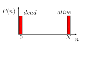
Figure 1: Signifying a cat-state by falsifying the quantum realism model (2). Measurements $\hat{M}$ on a system yield binary outputs. The Type I signature negates the model (2) for this system, where the quantum density operators $\rho_{1}$ and $\rho_{2}$ give the “dead” and “alive” results respectively.

Similar considerations give Type I signatures for the two-mode NOON superposition state

$$|\psi_{NOON}\rangle=\frac{1}{\sqrt{2}}\Bigl{(}|N\rangle_{A}|0\rangle_{B}+|0\rangle_{A}|N\rangle_{B}\Bigr{)}$$ (5)

that has been prepared in the laboratory opticalNOON-1 . The $\hat{a},$ $\hat{b}$ are boson destruction operators for two modes denoted $A$ and $B$, respectively. The $|n\rangle_{A}$ is the eigenstate of mode number $\hat{n}_{a}=\hat{a}^{\dagger}\hat{a}$ and similarly $|n\rangle_{B}$ is the eigenstate of $\hat{n}_{b}=\hat{b}^{\dagger}\hat{b}$. One can define $\hat{M}$ as the mode number difference $J_{z}=(\hat{n}_{a}-\hat{n}_{b})/2$. The binned regions $1$ and $2$ are those that give outcomes for $J_{z}$ as either negative or positive, respectively. Similar to the above case (3), the NOON state $|\psi_{NOON}\rangle$ predicts a binary distribution as in Figure 1. As one example of a Type I signature, the system prepared in a NOON state can be rigorously distinguished from all classical mixtures (2) by the observation of $\langle\hat{a}^{\dagger N}\hat{b}^{N}\rangle\neq 0$ bognoon ; murray . This moment has been measured by higher order interference fringe patterns as explained in Refs. opticalNOON-1 ; bognoon .

We conclude this section by noting that most previous approaches for signifying a Schrodinger cat-state use a Type I signature of some sort (though sometimes with additional assumptions) e.g. see Refs. ystbeamsplit-1-1 ; cats ; cats2 ; catsphil .

III Type II cat-signatures: Negating localised macroscopic hidden variable state realism

The next question is how to negate probabilistic classical mixtures where the cat-system can be “dead” or “alive”, without the assumption that the component states of the mixtures are necessarily quantum states. This question has been analysed in the literature, but different analyses have introduced different extra assumptions (e.g. we will compare Refs. LG ; svet ; MLR ; mdrmlr2 ; eprcat ; noonbellalex ). In this Section, we examine signatures for the cat-state based on the additional assumption of locality between the cat-system $C$ and a second remote system $S$.

III.1 Localised macroscopic hidden variable states

We consider Schrodinger’s original formulation of the cat-paradox, where the cat-system is entangled with a second system: A common example is cats

$$|\psi\rangle=\frac{1}{\sqrt{2}}\Bigl{(}|-\alpha\rangle_{C}|\downarrow\rangle_{S}+|\alpha\rangle_{C}|\uparrow\rangle_{S}\Bigr{)}$$ (6)

Here $|\uparrow\rangle$, $|\downarrow\rangle$ are the spin-$1/2$ eigenstates for $\hat{J}_{z}$ and the cat-system is modelled as the single bosonic mode in a coherent state $|\alpha\rangle$.

A second example is the Greenberger-Horne-Zeilinger (GHZ) state comprising $N$ spin-$1/2$ particles svetcats ; svet :

$$|\psi_{GHZ}\rangle=\frac{1}{\sqrt{2}}\Bigl{(}|\uparrow\rangle^{\otimes N}-|\downarrow\rangle^{\otimes N}\Bigr{)}$$ (7)

This system can be divided into two subsystems and written as

$$|\psi_{GHZ}\rangle=\frac{1}{\sqrt{2}}\Bigl{(}|\uparrow\rangle_{C}^{\otimes N-k}|\uparrow\rangle_{S}^{\otimes k}-|\downarrow\rangle_{C}^{\otimes N-k}|\downarrow\rangle_{S}^{\otimes(k)}\Bigr{)}$$ (8)

Here $|\uparrow\rangle^{\oplus N-k}=\prod_{m=1}^{N-k}|\uparrow\rangle^{(m)}$ and $|\uparrow\rangle^{\oplus k}=\prod_{m=N-k+1}^{N}|\uparrow\rangle^{(m)}$ where $|\uparrow\rangle^{(m)}$ is the spin eigenstate for $\hat{\sigma}_{Z}^{(m)}$, the $\hat{\sigma}_{Z}$ observable for the $m$-th particle. The $|\downarrow\rangle^{\oplus N-k}$ and $|\downarrow\rangle^{\oplus k}$ are defined similarly in terms of the eigenstates $|\downarrow\rangle$. The $\hat{\sigma}_{Z}$, $\hat{\sigma}_{X}$ and $\hat{\sigma}_{Y}$ are the Pauli spin observables. We classify the first $N-k$ particles as being part of the cat-system $C$ and the remaining $k$ particles as forming the second system denoted $S$. In this case, the measurement $\hat{M}$ is the collective spin $\sum_{m=1}^{N-k}\hat{\sigma}_{Z}^{(m)}$ of the cat-system $C$ and the “dead” and “alive” outcomes symbolised in Figure 1 correspond to the results $N-k$ and $-(N-k)$.

Another example of an entangled cat-system is the NOON state (5) where the mode $A$ is the cat-system $C$ and the mode $B$ is the system $S$. Here, $\hat{M}=\hat{n}_{a}$ and the dead and alive outcomes are numbers $0$ and $N$ as in Figure 1.

To describe a Schrodinger cat state without the assumption that the dead and alive states are quantum states, we assume a hidden variable model in which the cat-system $C$ is always either in a hidden variable state for which the cat is “dead”, or in a hidden variable state for which the cat is “alive”. These two hidden variable states need not be quantum states, which limits the criteria that can be applied to negate such a model. For example the Type 1 signature (4) that assumes the uncertainty relation for each dead and alive state is no longer useful. In order to derive suitable criteria, we introduce the further assumption of locality between the two systems $C$ and $S$ of the cat-states (6)-(8) and (5). We call such dead and alive hidden variable states (subject to the assumption of locality) localised macroscopic hidden variable states.

The locality assumption is based on the principle that the two subsystems, the “cat” $C$ and the spin $S$, can become spatially separated, so that measurements made on them can be space-like separated. The assumption of local hidden variables states implies that the joint probability for a result $x_{c}$ and $x_{s}$ upon measurements $X_{C}(\theta)$ and $X_{S}(\phi)$ on the cat and spin systems respectively can be written in the form of Bell’s local hidden variable model (LHV):

$$P(x_{c},x_{s})=\int\rho(\lambda)P_{C}(x_{c}|\theta,\lambda)P_{S}(x_{s}|\phi,\lambda)d\lambda$$ (9)

Here the hidden variable state is given by a set of variables denoted $\lambda$ and $\rho(\lambda)$ is the associated probability density. The $\theta$ and $\phi$ represent the choice of measurement made at $C\equiv A$ and $S\equiv B$. The $P_{C}(x_{c}|\theta,\lambda)$ and $P_{S}(x_{s}|\phi,\lambda)$ are probabilities for the outcome $x_{c}$ (or $x_{s}$) given the hidden state $\lambda$. The factorisation in the integrand reflects the locality assumption that the probability of the outcome at one site does not depend on the choice of measurement made at the other site.

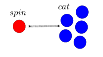
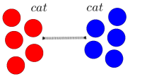
Figure 2: Signifying a Schrodinger cat-system (8) by falsifying all localised macroscopic hidden variable state (LMHVS) models (10). Locality is assumed between the two subsystems $S$ (red) and $C$ (blue), but not within each subsystem. The violation of the Svetlichny-type multipartite Bell inequality falsifies all such models for the GHZ state, including for the system of two cats (top right).

III.2 The macroscopic hidden variable $\lambda_{M}$: Correlation, LHV models and the macroscopic pointer

The premise of macroscopic realism (MR) for the cat-system $C$ places an additional restriction on the LHV model (9). For consistency with MR, each hidden variable state $\lambda_{M}$ comprises a macroscopic hidden variable, $\lambda_{M}$, which takes the value $+1$ if the cat-system is “alive”, and $-1$ if the cat-system is “dead”.

However, in the specific examples of the cat-states (6), (8) and (5), this condition does not have to be imposed because for these particular correlated states, it arises naturally as a consequence of the LHV assumption (9). In each case, there is a correlation between the systems $C$ and $S$, so that a measurement on the system $S$ will imply the outcome (whether “alive” or “dead”) for the cat-system $C$. For example, for the GHZ state (8) the value of $\hat{M}$ can be inferred from the collective spin measurement $\hat{O_{S}}=\sum_{m=N-k+1}^{N}\hat{\sigma}_{Z}^{(m)}$ of the system $S$. Similarly for the NOON state, the value of $\hat{M}=\hat{n}_{a}$ can be inferred from measurement $\hat{O}_{S}=\hat{n}_{b}$ on $S$. Consistency with the LHV model then imposes the condition that there be a macroscopic hidden variable $\lambda_{M}$, to denote that the for the cat-system $C$, the measurement $\hat{M}$ has a predetermined outcome i.e. that the “cat” is predetermined “dead” or “alive”. This result is proved in Ref. mdrcat but is part of the original analysis of “elements of reality” given by Einstein-Podolsky-Rosen epr .

To remind us of the need for consistency with MR, we rewrite the LHV model (9) as

$$P(x_{C},x_{S}) = \int\rho(\lambda,\lambda_{M})P_{C}(x_{c}|\theta,\lambda,\lambda_{M})$$ (10)

$$\ \ \ \ P_{S}(x_{s}|\phi,\lambda,\lambda_{M})d\lambda d\lambda_{M}$$

where we make the macroscopic hidden variable $\lambda_{M}$ explicit in the notation. We call this model a localised macroscopic hidden variable state model (LMHVS). We also note that this model for the quantum states (6), (8) and (5) is a model for a quantum measurement of the system $S$. The second system $C$ (the cat) acts as the measurement pointer of a measurement apparatus that measures an observable $\hat{O}_{S}$ of $S$. This is because the result for $\hat{M}$ (which gives the measured state of the “cat”, whether “dead” or “alive”) indicates the result of the measurement of the observable $\hat{O}_{S}$ of the first system $S$. The association in the model (10) of a macroscopic hidden variable $\lambda_{M}$ gives a theory in which the macroscopic pointer is pointing “either dead or alive” at all times.

III.3 Negating localised macroscopic hidden variable state realism

The negation of the LMHVS model (10) is possible using certain Bell inequalities. To avoid the issue about which hidden variable states are falsified (those of the cat system $C$ or the system $S$), we consider the entangled cat-states where both systems $A\equiv C$ and $B\equiv S$ are large. Specifically, we consider the GHZ state comprising $N$ spin-$1/2$ particles as two separated spin-systems (Figure 2b) where both $k$ and $N-k$ are large. The negation of the LHV model (9) for this system would tell us that there can be no hidden variable state for each subsystem that is consistent with locality between the two systems $C$ and $S$. In particular, this negates that there can be any mixture for (at least one of) the cat systems which enable the cat to be in a “dead” or “alive” local state.

For a system prepared in the GHZ state (8), the negation of the LMHVS (10) can be proved using Svetlichny Bell inequalities derived in Refs. svet . To summarise, consider the complex operator $\Pi_{M}=\prod_{j=1}^{M}F_{j}$, $M\leq N$ where $F_{j}=\sigma_{X}^{(j)}+i\sigma_{Y}^{(j)}$ ($j\neq N$) at each of the sites and $F_{N}=\sigma_{\pi/4}^{(N)}+i\sigma_{3\pi/4}^{(N)}$ ($\sigma_{\theta}^{(j)}=\sigma_{X}^{(j)}\cos\theta+\sigma_{Y}^{(j)}\sin\theta$). Observables $\mathrm{Re}\Pi_{M}$ and $\mathrm{Im}\Pi_{M}$ are defined according to $\Pi_{M}=\mathrm{Re}\Pi_{M}+i\mathrm{Im}\Pi_{M}$. That there cannot be a hidden variable set consistent the LMHVS model (10) is proved using the fact that there are algebraic bounds $\langle\mathrm{Re}\Pi_{M}\rangle,\langle\mathrm{Im}\Pi_{M}\rangle\leq 2^{M-1}$ and $\langle\mathrm{Re}\Pi_{M}\rangle+\langle\mathrm{Im}\Pi_{M}\rangle\leq 2^{M}$ for any such underlying hidden variable state. The LHV model leads to the Svetlichny-Bell inequality svet

$$\langle\mathrm{Re}\Pi_{N}\rangle+\langle\mathrm{Im}\Pi_{N}\rangle\leq 2^{N-1}$$ (11)

The inequalities are predicted to be violated by the GHZ state, which gives the prediction

$$\langle\mathrm{Re}\Pi_{N}\rangle+\langle\mathrm{Im}\Pi_{N}\rangle=2^{N-1/2}$$ (12)

In fact the violation holds for all bipartitions (8) of the $N$ spin systems i.e. for all values of $k$. In this way, we see that we negate any hidden variable model for the “cat” system of any size, conditional that the state be consistent with the locality assumption between the two (potentially macroscopic) systems $C$ and $S$.

Other Bell inequalities have been constructed that could be applied to negate the LMHVS model for the NOON state (5) and the entangled cat-state noonbellalex

$$|\psi\rangle=\frac{1}{\sqrt{2}}\{|-\alpha\rangle|-\alpha\rangle+|\alpha\rangle|\alpha\rangle\}$$ (13)

These violations have been tested in some experimental situations bellcatexp . Such violations demonstrate the failure of any hidden variable state to describe a cat-system, given that this state must be consistent with the assumption of locality between the cat-system $C$ and a second system $S$.

IV Interpreting the Type I and II cat-signatures

IV.1 Microscopic effects

If a Type I or II cat-signature is observed in an experiment, then it cannot be ruled out that the signature is due to a microscopic quantum effect. This is because the Type I and II cat-signatures involve predictions for measurements other than the macroscopic measurement $\hat{M}$. In order to signify the cat-state using these signatures, it is necessary to make assumptions about the microscopic predictions for these measurements $-$ for example that they are consistent with locality down to a single atom or photon level. The consequence is that the Type I and II cat-signatures are not sufficient to negate the validity of the macroscopic hidden variable $\lambda_{M}$ mdrcat .

To illustrate, the Type I signature given by $\langle\hat{a}^{\dagger N}\hat{b}^{N}\rangle\neq 0$ for the NOON state is observable as an interference pattern with frequency proportional to $N$ (see Refs. opticalNOON-1 ). The pattern is increasingly difficult to resolve as $N\rightarrow\infty$ e.g. all photons need to be detected at either one location or another. (See Ref. gisinuncert for more general results).

Similarly, the Type II signature given by the violation of the Svetlichny Bell inequality (11) requires measurement of the spins $\hat{\sigma}_{X}$, $\hat{\sigma}_{Y}$ of all the $N$ particles. To negate the hidden variable model (10), it is therefore necessary to assume that the hidden variable states $\lambda$ give predictions for microscopic features of the cat-system. Bounds on the detail required to signify certain cat-states by a Type II signature have been given in Ref. MLR-uncert ; mdrcat where it is shown that a measurement resolution at the quantum noise level is necessary.

To summarise: The Type I and II signatures of the cat-state are a negation that the cat is in an alive or dead state, where the meaning of “state” is that the “state” gives microscopic details in the predictions of measurements made on the cat-system. e.g. the Type II signatures are a negation of the hidden variable states that give microscopic detail in the predictions. Thus, if we signify the cat-state, we can only say that the cat is neither in a dead state, nor in an alive state, where the “state” means a description of the system that gives microscopic details of certain measurements.

IV.2 Macroscopic pointer

Bearing in mind that the macroscopic hidden variable predetermines the result for the macroscopic measurement, if we cannot negate the macroscopic hidden variable $\lambda_{M}$, then the simplest interpretation is that the cat was indeed “dead” or “alive” prior to the measurement, and that the signature of the cat-state is evidence of failure of the assumptions made about the microscopic predictions for the system mdrcat .

For example, it cannot be excluded that the signatures are due to a microscopic nonlocal effect. The LHV model (10) assumes full locality between the two systems $C$ and $S$. If this full locality is relaxed by a small amount (to allow small changes of size $\delta$ in the cat-state due to measurements on the spin), then the signature of the cat-state is nullified.

The interpretation is depicted in Figure 3. Here, the macroscopic pointer does indeed point to one of two macroscopically distinct locations $x_{1}$ and $x_{2}$ on a measurement dial. In terms of the state (6), the positions represent the $\hat{x}$ outcomes $x_{1}$ and $x_{2}$ corresponding to the coherent states $|\alpha\rangle$ or $|-\alpha\rangle$ respectively ($\alpha$ is real). The positions are not defined with a microscopic precision, however, and the pointer may have an indeterminacy $\delta$ in position/ momenta. This is associated with a potential nonlocal effect of size $\delta$.

In the context of many cat-signatures (see Refs. mdrcat ; mdrmlr2 ; MLR-uncert ; ystbeamsplit-1-1 ), “microscopic” implies a size $\delta$ of an order defined by the Heisenberg uncertainty bound. In the above, the addition of noise $\delta_{x}$ and $\delta_{p}$ to the measurements of $x$ and $p$ where $\delta_{x}\delta_{p}\sim 1/2$ is known to destroy the quantum effect $-$namely, the signature of the cat MLR-uncert .

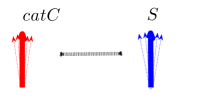
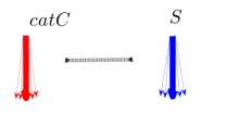
Figure 3: Macroscopic pointer: The pointer in a quantum measurement process is modelled as the cat-system $C$ of the cat-state (1). The system being measured is modelled as the spin-system $S$. When a measurement of the spin $\sigma_{Z}$ occurs, there are two final positions for the pointer. While a possible quantum interpretation of the cat-state is that the pointer is “simultaneously in both positions”, the Type I and II signatures of the cat-state cannot negate the macroscopic hidden variable $\lambda_{M}$ that predetermines the pointer to be at one location or the other. It cannot be excluded that the Type II signature is due to microscopic nonlocal effects of size $\sim\delta$ between the pointer $C$ and the spin $S$ (lower diagram). The cat-state is consistent with the pointer being in one position or the other (though with a microscopic indeterminacy associated with the microscopic nonlocality).

V Type III cat-signatures: Negating macroscopic local realism

A strong way to signify a Schrodinger cat-state is to falsify the macroscopic hidden variable $\lambda_{M}$. Since this hidden variable is a predetermination of the macroscopic measurement $M$ only (not other measurements), the falsification of this variable would imply a genuine negation of “macroscopic reality (MR)”. In that case, one can say the “cat” is neither dead nor alive, where this means the measurement outcome for $\hat{M}$ is not predetermined, in analogy with interpretation discusssed in Schrodinger’s essay. There have been proposals to falsify MR by negating the macroscopic hidden variable $\lambda_{M}$, a well-known example being the Leggett-Garg proposal LG . This proposal however involves a second premise. Logically, wherever a second premise is introduced, it is necessary to examine the second premise closely, since a signature can occur if the second premise fails, with the first premise (macroscopic realism) being upheld.

In this Section, we examine an alternative test of macroscopic realism, one in which macroscopic realism is defined in conjunction with the second premise of macroscopic locality. This means that we consider two spatially separated systems $A$ and $B$, and spacelike separated measurements made on each one. The combined premise we refer to as macroscopic local realism (MLR). We argue that the premise of macroscopic locality is a suitable co-premise of macroscopic realism, in that the falsification of MLR is as significant as falsification of MR.

V.1 Bell Inequalities for MLR

The premise of MLR combines the premises of macroscopic realism and macroscopic locality. Macroscopic realism is that the system $A$ (or $B$) is in one of two macroscopically distinguishable states at all time, in the sense of the macroscopic hidden variable $\lambda_{M}^{A}$ (or $\lambda_{M}^{B}$) being predetermined. It is thus assumed that a measurement $\hat{M}^{A}$ made on system $A$ reads out the value of the hidden variable $\lambda_{M}^{A}$, defined with a macroscopic degree of fuzziness; and similarly for a measurement $\hat{M}^{B}$ at $B$. Macroscopic locality is that the measurement $\hat{M}$ on one system cannot bring about an immediate macroscopic change to the system at the other location. By a macroscopic change in this context, we mean a transition of the macroscopic hidden variable $\lambda_{M}$ being $+1$ to being $-1$ or vice versa i.e. a transition between “dead” and “alive”. The premise of macroscopic locality asserts that a measurement cannot make a macroscopic change to another system, but we cannot exclude that it can make a microscopic one. The premise is therefore less strict than the premise of locality (or local realism) which excludes all changes, microscopic and macroscopic, and which has been negated.

Let us consider two spatially separated systems $A$ and $B$ and spacelike separated measurements $\hat{M}_{\theta}^{A}$ and $\hat{M}_{\phi}^{B}$ that can be made on each system. Here $\theta$ and $\phi$ are measurement settings and we consider two measurement choices $\theta$, $\theta^{\prime}$ and $\phi$, $\phi^{\prime}$ for each system. We suppose that the measurements $\hat{M}_{\theta}^{A}$, $\hat{M}_{\theta^{\prime}}^{A}$ and $\hat{M}_{\phi^{\prime}}^{B}$, $\hat{M}_{\phi}^{B}$ each give macroscopically distinct binary outcomes which are denoted $+1$ and $-1$ (corresponding to “alive” and “dead” regimes 2 and 1 shown in Figure 4). If we assume macroscopic local realism, the following CHSH Bell inequality will hold MLR

$$\langle\hat{M}_{\theta}^{A}\hat{M}_{\phi}^{B}\rangle-\langle\hat{M}_{\theta}^{A}\hat{M}_{\phi^{\prime}}^{B}\rangle+\langle\hat{M}_{\theta^{\prime}}^{A}\hat{M}_{\phi}^{B}\rangle+\langle\hat{M}_{\theta^{\prime}}^{A}\hat{M}_{\phi^{\prime}}^{B}\rangle \leq 2$$

The MLR model is an example of an LHV model and the derivation of (LABEL:eq:bell-1) is therefore that of the standard CHSH Bell inequality that applies to all LHV models where the measurements have binary outcomes CHSHBell . The violation of (LABEL:eq:bell-1) will imply failure of MLR. Violations of Bell inequalities for cat-states have been predicted and observed experimentally bellcatexp ; noonbellalex ; svetcats . However these do not involve macroscopic outcomes for all measurements $\theta$, $\theta^{\prime}$, $\phi$ and $\phi^{\prime}$ and hence do not violate (LABEL:eq:bell-1). That signatures of a cat-state require at least one measurement to be finely resolved is a generic property discussed in Refs gisinuncert ; mdrcat ; ystbeamsplit-1-1 . This would seem to make the violation of (LABEL:eq:bell-1) impossible.

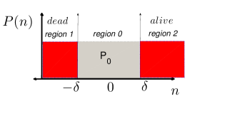
Figure 4: Practical method for testing $\delta$-scopic LR. The outcomes of each measurement indicated in Figure 5 is binned into one of the regions $1,0,2$. As $\alpha\rightarrow\infty$, $P_{0}\rightarrow 0$.

As might be expected, however, the possibility of violating the inequality (LABEL:eq:bell-1) depends on how we interpret “macroscopic”. First, we generalise the definition of MLR by defining $\delta$-scopic local realism ($\delta$-LR). The $\delta$-scopic LR is falsified where the separation between the outcomes for the measurements $\hat{M}_{\theta}^{A}$, $\hat{M}_{\theta^{\prime}}^{A}$ and $\hat{M}_{\phi^{\prime}}$, $\hat{M}_{\phi}^{B}$ is greater than or equal to $2\delta$ (Figure 4). We next examine scenarios where it may be possible to falsify $\delta$-scopic local realism for some quantifiable $\delta$ that can be made large by an amplification process that involves measurement of quantum noise. In the scenarios that we consider, the amplifcation process occurs as part of a measurement process, similar to the Schrodinger-cat gedanken experiment.

V.2 Amplification of the quantum noise level

We now consider in detail proposals that have been put forward for violating $\delta$-scopic local realism using field quadrature phase amplitude observables. The crucial point is that measurement of the field amplitudes takes place via an amplification process that involves a second field, so that the final measurement is of a Schwinger spin mdrmlr2 ; MLR . The uncertainty principle for spin is

$$\Delta\hat{J}_{X}^{A}\Delta\hat{J}_{Y}^{A}\geq|\langle\hat{J}_{Z}^{A}\rangle|/2$$ (15)

One is able to create a situation where the quantum noise level given by $|\langle\hat{J}_{Z}^{A}\rangle|/2$ is amplified to a very large photon number difference (field intensity). This allows consideration of changes of order $\delta$ where $\delta$ is large in the absolute sense of particle number (intensity) but small compared to the quantum noise level. The highly non-classical mesoscopic effects that are predicted can then be understood as a property of amplified quantum fluctuations.

The system we consider comprises two spatially separated modes at $A$ and $B$ (Figure 5). We denote the modes at $A$ and $B$ by the boson operators, $\hat{a}_{1}$ and $\hat{b}_{1}$, respectively. At each location, the mode $\hat{a}_{1}$ (or $\hat{b}_{1}$) is combined with a second mode $\hat{a}_{2}$ (or $\hat{b}_{2}$) respectively. This combination can occur through a $50/50$ beam splitter. The outputs at each location are rotated modes with boson operators given as $\hat{c}_{+}=(\hat{a}_{1}+\hat{a}_{2})\sqrt{2}$ and $\hat{c}_{-}=(-\hat{a}_{1}+\hat{a}_{2})/\sqrt{2}$ for $A$, and $\hat{d}_{+}=(\hat{b}_{1}+\hat{b}_{2})/\sqrt{2}$ and $\hat{d}_{-}=(-\hat{b}_{1}+\hat{b}_{2})/\sqrt{2}$ for $B$. At each location, an experimentalist makes a measurement of a number difference $N_{+}-N_{-}$ defined

$$\hat{J}_{\theta}^{A}(\varphi)=(N_{+}-N_{-})/2=(\hat{c}_{2}^{\dagger}\hat{c}_{2}-\hat{c}_{1}^{\dagger}\hat{c}_{1})/2$$ (16)

where $\hat{c}_{2}=\hat{c}{}_{+}\cos\theta+e^{i\varphi}\hat{c}_{1}\sin\theta$ and $\hat{c}_{1}=-\hat{c}_{+}\sin\theta+e^{i\varphi}\hat{c}_{-}\cos\theta$. This could be carried out using a phase shift $\varphi$ and polarising beam splitters rotated to $\theta$ with the modes $c_{+}$ and $c_{-}$ as inputs. The measurement (16) corresponds to a measurement of the Schwinger spin observables $\hat{J}_{X}^{A}$, $\hat{J}_{Y}^{A}$, $\hat{J}_{Z}^{A}$ at $A$ for the operators $a_{1}$ and $a_{2}$.

$$\hat{J}_{X}^{A}=\hat{J}_{0}^{A}(\varphi) = (\hat{a}_{2}^{\dagger}\hat{a}_{1}+\hat{a}_{1}^{\dagger}\hat{a}_{2})/2$$

$$J_{Y}^{A}=\hat{J}_{\pi/4}(\pi/2) = (\hat{a}_{2}^{\dagger}\hat{a}_{1}-\hat{a}_{1}^{\dagger}\hat{a}_{2})/(2i)$$

$$\hat{J}_{Z}=\hat{J}_{\pi/4}(0) = (\hat{a}_{2}^{\dagger}\hat{a}_{2}-\hat{a}_{1}^{\dagger}\hat{a}_{1})/2$$ (17)

The spin observables at $B$ are defined similarly as

$$\hat{J}_{\phi}^{B}(\gamma)=(\hat{d}_{2}^{\dagger}\hat{d}_{2}-\hat{d}_{1}^{\dagger}\hat{d}_{1})/2$$ (18)

where $\hat{d}_{2}=\hat{d}{}_{+}\cos\phi+e^{i\gamma}\hat{d}{}_{-}\sin\phi$ and $\hat{d}_{1}=-\hat{d}_{+}\sin\varphi+e^{i\gamma}\hat{d}_{-}\cos\varphi$. We define the Schwinger observables at $B$ as $\hat{J}_{X}^{B}=(\hat{b}_{2}^{\dagger}\hat{b}_{1}+\hat{b}_{1}^{\dagger}\hat{b}_{2})/2$, $\hat{J}_{Y}^{B}=(\hat{b}_{2}^{\dagger}\hat{b}_{1}-\hat{b}_{1}^{\dagger}\hat{b}_{2})/(2i)$ and $\hat{J}_{Z}^{B}=(\hat{b}_{2}^{\dagger}\hat{b}_{2}-\hat{b}_{1}^{\dagger}\hat{b}_{1})/2$.

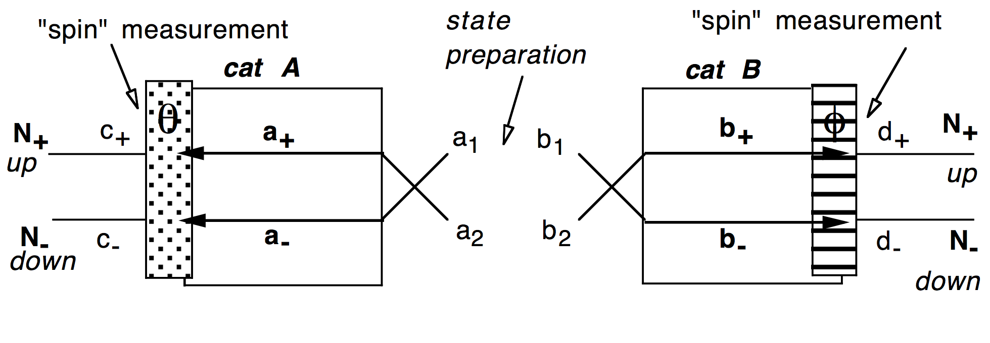
Figure 5: Two Schrodinger cat-type states created as part of the measurement process: The modes $a_{1}$ and $b_{1}$ are created in an entangled state $|\psi\rangle$. The final measurement of the number difference $J=(N_{+}-N_{-})/2$ at each detector is an “amplified” value of the quadrature phase amplitudes $x_{\theta}$ and $x_{\phi}$ of the fields $a_{1}$ and $b_{1}$. The amplifcation is created at the beam splitter where the fields $a_{2}$ and $b_{2}$ are independent intense coherent states $|\alpha\rangle$. A Schrodinger cat-type system is then created at each site $A$ and $B$.

Experiments have been performed where the modes $a_{1}$ and $b_{1}$ are created in an entangled state and the fields $a_{2}$ and $b_{2}$ are (to a good approximation) intense classical fields of amplitude $\alpha$ (which we take to be real), similar to local oscillator fields polsqueezing ; polsqother . Thus, each of the modes $c_{\pm}$ prior to the polarisation measurement $\hat{J}_{\theta}^{A}(\varphi)$ has (potentially) a macroscopic photon number (and similarly for the fields at $B$). In the experiments, a final polarisation entanglement between the fields at $A$ and $B$ is signified via measurements of $\hat{J}_{\theta}^{A}(\varphi)$ and $\hat{J}_{\phi}^{B}(\gamma)$. The measurements $\hat{J}_{\theta}^{A}(\varphi)$ and $\hat{J}_{\phi}^{B}(\gamma)$ are also measurements of the quadrature phase amplitudes $\hat{x},\hat{p}$ of the original modes $a_{1}$ and $b_{1}$. This is because we can simplify:

$$\hat{J}_{X}^{A}=\hat{J}_{0}^{A}(\pi/2) = \alpha(a_{1}+a_{1}^{\dagger})/2=\alpha\sqrt{2}\hat{x}^{A}$$

$$\hat{J}_{Y}^{A}=\hat{J}_{\pi/4}(\pi/2) = \alpha(a_{1}-a_{1}^{\dagger})/(2i)=\alpha\sqrt{2}\hat{p}^{A}$$

$$\hat{J}_{Z}=\hat{J}_{\pi/4}(0) = \alpha^{2}/2$$ (19)

where $\hat{x}^{A}=(\hat{a}_{1}^{\dagger}+\hat{a}_{1})/\sqrt{2}$ and $\hat{p}^{A}=i(a_{1}^{\dagger}-a_{1})/\sqrt{2}$. The Heisenberg uncertainty relation is $\Delta\hat{x}^{A}\Delta\hat{p}^{A}\geq 1/2$. A similar result holds for the quadrature phase amplitudes $\hat{x}^{B}=(\hat{b}_{1}^{\dagger}+\hat{b}_{1})/\sqrt{2}$ and $\hat{p}^{B}=i(\hat{b}_{1}^{\dagger}-\hat{b}_{1})/\sqrt{2}$ defined at $B$. In fact $\hat{J}_{\theta}(\pi/2)=\alpha\sqrt{2}\hat{x}_{2\theta}^{A}$ where $\hat{x}_{\theta}=\hat{x}\cos\theta+\hat{p}\sin\theta$.

We envisage an experiment where at site $A$, the experimentalist can measure either $\hat{J}_{X}^{A}=\hat{J}_{0}^{A}(\pi/2)$ or $\hat{J}_{Y}^{A}=\hat{J}_{\pi/4}(\pi/2)$. In terms of the original fields, using the result (19), this corresponds to either $\alpha\sqrt{2}\hat{x}^{A}$ or $\alpha\sqrt{2}\hat{p}^{A}$. Each of $\hat{J}_{X}^{A}$ and $\hat{J}_{Y}^{A}$ is a measurement of a particle number difference according to the expression (18). The choice of whether to measure $\hat{J}_{X}$ or $\hat{J}_{Y}$ is made after the combination of the mode $a_{1}$ with the strong field $a_{2}$. The $\hat{J}_{X}^{A}$ and $\hat{J}_{Y}^{A}$ are thus measurements of the amplified quadrature phase amplitudes $\alpha\sqrt{2}\hat{x}^{A}$ and $\alpha\sqrt{2}\hat{p}^{A}$. Similar measurements are made at $B$, where one would measure either $\alpha\sqrt{2}\hat{x}^{A}$ or $\alpha\sqrt{2}\hat{p}^{A}$. Hence if one considers a change $\delta_{X}$ (or $\delta_{P}$) in the quadrature phase amplitude $\hat{X}$ (or $\hat{P}$), one can define in this context an amplified change $\delta=\alpha\sqrt{2}\delta_{X}$ (or $\alpha\sqrt{2}\delta_{P}$) for the particle number difference measured by $\hat{J}_{X}$ (or $\hat{J}_{Y}$). The change can be made arbitrarily large, in an absolute sense, by increasing $\alpha$.

We note the increase in $\alpha$ also amplifies the total number of particles at each site (this being determined by $|\alpha|^{2}$). The nature of the amplification is evident by the uncertainty relation (15) for the actual spin measurements which reduces in this case to

$$\Delta\hat{J}_{X}^{A}\Delta\hat{J}_{Y}^{A}\geq|\alpha|^{2}/4$$ (20)

since $\alpha$ is taken to be very large. The amplification that is crucial to creating the macroscopic states at the locations $A$ and $B$ is also an amplification of the quantum noise level, and there is no amplification relative to this level.

V.3 Using states that violate Continuous Variable Bell inequalities

One can now design experiments that are predicted to falsify a $\delta$-scopic local realism. For some states, the correlations obtained for the quadrature phase amplitude measurements $\hat{x}_{\theta}^{A}$ and $\hat{x}_{\phi}^{B}$ at each site are predicted to violate a Bell inequality. The outcome $x$ for the measurement $\hat{x}$ at each site can be binned into regions of positive and negative values. We define an observable $\hat{S}_{\theta}^{A}$ whose value is $+1$ if $x_{\theta}^{A}\geq 0$ and $-1$ otherwise. A similar observable $\hat{S}_{\phi}^{B}$ is defined at $B$, based on the quadrature phase amplitude $\hat{x}_{\phi}^{B}$. It has been shown that for certain states $|\psi\rangle$ and for certain angles $\phi$, $\phi^{\prime}$, $\theta^{\prime}$ and $\theta$, the following Bell inequality is violated

$$E=\langle S_{\theta}^{A}S_{\phi}^{B}\rangle-\langle S_{\theta}^{A}S_{\phi^{\prime}}^{B}\rangle+\langle S_{\theta^{\prime}}^{A}S_{\phi}^{B}\rangle+\langle S_{\theta^{\prime}}^{A}S_{\phi^{\prime}}^{B}\rangle\leq 2$$ (21)

thus negating the possibility of an LHV model describing the results of those measurements. Since we can also write $\hat{J}_{\theta}^{A}=\alpha\sqrt{2}\hat{x}_{2\theta}^{A}$ and $\hat{J}_{\phi}^{B}=\alpha\sqrt{2}\hat{x}_{2\phi}^{B}$, this inequality is also violated if we define $\hat{S}_{\theta}^{A}$ as the observable with value $+1$ if $J_{\theta}^{A}\geq 0$ and $-1$ otherwise and $\hat{S}_{\phi}^{B}$ as the observable with value $+1$ if $J_{\phi}^{B}\geq 0$ and $-1$ otherwise. The violation implies that there is no predetermined (local) hidden variable description for the sign of the number differences $J_{\theta}^{A}$, $J_{\phi}^{B}$. This has been pointed out in the Ref. mdrmlr2 . Because we can amplify $\alpha$, this gives a situation whereby one can falsify local hidden variables for measurements of particle number difference that can tolerate an uncertainty (or poor resolution) that increases as $\alpha$ increases, the uncertainty becoming macroscopic as $\alpha\rightarrow\infty$. An example of the state $|\psi\rangle$ is the pair coherent state

$$|\psi\rangle=\frac{e^{r_{0}^{2}}}{2\pi\sqrt{I_{0}(2r_{0}^{2})}}\int_{0}^{2\pi}|r_{0}e^{i\zeta}\rangle|r_{0}e^{-i\zeta}\rangle d\zeta$$ (22)

($I_{0}$ is the modifed Bessel function, $r_{0}=1.1$) that is generated near the threshold of nondegenerate parametric oscillation pair-coh .

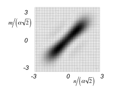
Figure 6: Signature of the Schrodinger cat state created by apparatus of Figure 4: The number differences $J=(N_{+}-N_{-})/2$ at the site $A$ and $B$ are denoted $n$ and $m$ respectively, and are binned to the values $S=1$ or $-1$ according to sign as described in text. Left: The expectation values $E$ violate the Bell inequality (21) for all $\alpha\rightarrow\infty$. Right: A contour graph of the probability for joint outputs $n$ and $m$. The absolute values of the number difference outputs $n$, $m$ increase with $\alpha$.

As $\alpha$ increases, we argue that the $+1$ and $-1$ outcomes for $\hat{S}_{\theta}^{A}$ ultimately become macroscopically distinct (and similarly the $+1$, $-1$ outcomes for $\hat{S}_{\phi}^{B}$ become macroscopically distinct). The measurements $\hat{S}_{\theta}^{A}$ and $\hat{S}_{\phi}^{B}$ are then examples of macroscopic measurements $\hat{M}_{\theta}^{A}$ and $\hat{M}_{\phi}^{B}$ and the violation of (21) is a violation of (LABEL:eq:bell-1). In this limit we would violate “macroscopic local realism”.

To understand the argument, we define a region of measurement outcome $x$ for $\hat{J}_{\theta}^{A}$ where the result falls between $-\delta$ and $+\delta$ for some $\delta\neq 0$ (see Figure 4). We call this region $0$, and also define the region of outcome $x\geq\delta$ as region $2$, and the region of outcome $x\leq-\delta$ as region $1$. Then for fixed $\delta$, the probability $P_{0}$ of a result in the region $0$ becomes zero as $\alpha\rightarrow\infty$. Yet the violation of the Bell inequality is unchanged with $\alpha$ (Figure 6). Hence, violation of the inequality (LABEL:eq:bell-1) is possible for the two outcomes $+1$ and $-1$ that for large enough $\alpha$ can be justified as separated by a region of width $2\delta$. This is true for any arbitrarily large fixed $\delta$, because $\alpha$ can be made larger without altering the Bell violation. Hence, there is a prediction for a violation of mesoscopic/ macroscopic local realism.

The violation of the inequality (21) would imply a violation of $\delta-$scopic local realism where $2\delta$ is the separation between the outcomes $+$ and $-1$. For a realisation of the experiment, however, there will be a small nonzero probability for a result in the region $0$ and this must be taken into account. A method for doing this is explained in the next section.

V.4 Practical quantifiable $\delta$-scopic local realism tests

The macroscopic realism premise (MR) would apply if $\delta$ is macroscopic and $P_{0}=0$. Then MR asserts that if we consider two states with outcomes confined to regions $1$ and $2$ respectively, the system must be in a probabilistic mixture of those two states. The meaning of MR for the more general case where $P_{0}\neq 1$ is discussed in the paper of Leggett and Garg LG and further in Refs. eric_marg ; lauralg ; bognoon .

The MR premise for this generalised case is that the system be described as a probabilistic mixture of two overlapping states: the first gives outcomes in regions “$1$” or “$0$”; the second gives outcomes in regions “$0$” or “$2$”. The MR assumption excludes the possibility that the system can be in a superposition of two states, one that gives outcomes in region $1$ and the second that gives outcomes in $2$. It does not however exclude superpositions of states with outcomes in region 1 and 0, or superpositions of states with outcomes in regions 0 and 2. Where $\delta$ is finite and not necessarily macroscopic, we use the term $\delta$LR to describe the premise that is used.

We follow the approach of Ref. lauralg , and denote the hidden variable state associated with the outcomes in regions “$1$” or “$0$” for the system at $A$ by the variable $\tilde{S}^{A}=-1$ and the hidden variable state that generates outcomes in regions “0” and “2” by $\tilde{S}^{A}=1$. We define the variable $\tilde{S}^{B}$ similarly. The macroscopic locality assumption applies to assert that the measurement at one location cannot change the result at the other in such a way that the system changes value of $\tilde{S}$ from $+1$ to $-1$, vice versa. We can define $P_{+}$ and $P_{-}$ as the probability that the system is in the state with $\tilde{S}=+1$ or the other state with $\tilde{S}=-1$. Then we note that the $\delta$-LR assumptions would predict the Bell inequality

$$E = \langle\tilde{S}_{\theta}^{A}\tilde{S}_{\phi}^{B}\rangle-\langle\tilde{S}_{\theta}^{A}\tilde{S}_{\phi^{\prime}}^{B}\rangle+\langle\tilde{S}_{\theta^{\prime}}^{A}\tilde{S}_{\phi}^{B}\rangle+\langle\tilde{S}_{\theta^{\prime}}^{A}\tilde{S}_{\phi^{\prime}}^{B}\rangle\leq 2$$

However, the moments $K_{\theta\phi}=\langle\tilde{S}_{\theta}^{A}\tilde{S}_{\phi}^{B}\rangle$ are no longer directly measurable, because an outcome between $-\delta$ and $+\delta$ could arise from either state, $\tilde{S}=-1$ or $+1$. However, we can always conclude that $P_{1}\leq P_{-}\leq P_{1}+P_{0}$ and $P_{2}\leq P_{+}\leq P_{2}+P_{0}$, where $P_{1},$ $P_{2}$ and $P_{0}$ are the measurable probabilities of obtaining a result in regions $1$, $2$ and $0$ respectively (Figure 4). Hence, we establish bounds on the correlations assuming $\delta$LR, even if the $P_{0}$ are measured to have a nonzero probability. The modified inequality is

$$E_{\delta}=K_{\theta,\phi}^{lower}-K_{\theta\phi^{\prime}}^{upper}+K_{\theta^{\prime}\phi}^{lower}+K_{\theta^{\prime}\phi^{\prime}}^{lower}\leq 2$$ (24)

where $K_{\theta\phi}^{lower}$ and $K_{\theta\phi}^{upper}$ are lower and upper bounds to $K_{\theta\phi}$ i.e. $K_{\theta\phi}^{lower}\leq K_{\theta\phi}\leq K_{\theta\phi}^{upper}$. We see that $K_{\theta\phi}^{lower}=P_{2,2}(\theta,\phi)+P_{1,1}(\theta,\phi)-P_{10,20}(\theta,\phi)-P_{20,10}(\theta,\phi)$ and $K_{\theta\phi}^{upper}=P_{20,20}(\theta,\phi)+P_{10,10}(\theta,\phi)-P_{1,2}(\theta,\phi)-P_{2,1}(\theta,\phi)$. We introduce the notation that $P_{20,10}$, for example, is the joint probability for an outcome $J_{z}$ in regions $2$ or $0$ at $A$ with the measurement angle set at $\theta$ and an outcome $x$ in $1$ or $0$ at $B$ with the measurement angle set at $\phi$.

The modified inequality (24) gives a practical means to demonstrate a violation of an $\delta$-scopic local realism for a finite $\delta$ where there is a small probability $P_{0}$ of an outcome in the region defined by $-\delta<x<\delta$. A similar inequality has been derived for Leggett-Garg experiments lauralg . For realistic tests based on current experiments, the shifts $\delta$ may not be macroscopic, but nonetheless offer a route to test local realism beyond the single particle level considered in experiments so far.

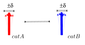
Figure 7: Macroscopic pointers: The macroscopic observables $J_{\theta}$, $J_{\phi}$ for two cat-systems $A$ and $B$ depicted in Figure 5 are the macroscopic pointers for the quadrature phase amplitude measurements of the microscopic systems $a_{1}$ and $b_{1}$. The violation of the inequality (24) reveals a nonlocal effect of size $\delta$ between the two pointers. This provides a test in which the signature negates a genuine indeterminacy of the position of the pointer, to within the $\pm\delta$. The size of $\delta$ can be amplified by increasing the value of the coherent amplitude $\alpha$. However, the indeterminacy is at the quantum noise level, and the two pointers are not correlated at that level.

V.5 The macroscopic pointers

In the experiment of Figure 5, the two cat-states at $A$ and $B$ act as two pointers for the microscopic quadrature phase amplitudes of the original entangled field modes denoted $a_{1}$ and $a_{2}$. There is a correlation between the “position” $J$ of each pointer as indicated by a particle number difference $N_{+}-N_{-}$ and the original amplitude of the mode. However, the “positions” of the two pointers are not well-correlated i.e. one pointer does not accurately measure the position of the other, at least not to a precision given by the quantum noise level of the uncertainty relation (20). This is evident by the plot of Figure 6b which shows a weak correlation between the quadrature phase amplitudes at each location. While the pointers are entangled, they are not well-correlated: The range of positions over which a pointer become interpretable as “being in simultaneously in both places” (or else shifted between those two places by measurements on a second pointer) is at this quantum noise level.

VI Discussion and Conclusion

In summary we have examined different approaches to signifying a Schrodinger cat-state, and contrasted with testing macroscopic realism. In Section II we considered a model of a cat-system in which the cat is described as a probabilistic mixture of two distinguishable quantum states, one describing the “cat” being “dead” and the other the “cat” being “alive”. Criteria to negate this model (which we call macroscopic quantum realism MQR) were derived in the form of inequalities based on the assumption that uncertainty relations hold for all quantum states. We called this negation a Type I signature of a cat-state.

In Section III we examined models for the cat-system that do not require the dead and alive states of the cat to be quantum states, but rather allow them to be hidden variable states subject to the condition of locality between the cat-system and a second remote system $S$. We called this model a localised macroscopic hidden variable state model (LMHVS). Criteria to negate the LMVS model were called Type II signatures, and included the violation of multipartite Bell inequalities.

It was explained in Section IV that both the MQR and LMHVS models make assumptions about microscopic predictions for measurements. Hence the Type I and Type II signatures do not directly falsify macroscopic realism. Macroscopic realism (MR) asserts that the cat is predetermined dead or alive, prior to a coarse-grained measurement $\hat{M}$ that distinguishes whether the cat is dead or alive (without measurement of the other details of the system). Macroscopic realism therefore asserts the validity of a macroscopic hidden variable $\lambda_{M}$ to describe the system: the $\lambda_{M}$ predetermines whether the cat will be measured dead or alive according to a measurement $\hat{M}$. Both the MQR and LMHVS models incorporate the macroscopic hidden variable $\lambda_{M}$, but also assume other hidden variables that give a predetermination for other measurements that are finely resolved. We cannot therefore exclude that the results of an experiment signifying the cat-state are caused by a microscopic nonlocal effect (such as a change of spin of one of the particles in a GHZ state) rather than a failure of MR.

In Section IV, we considered the classic example where the cat-system $C$ models the macroscopic pointer of a measurement apparatus that measures the spin of system $S$. After a measurement interaction, quantum theory predicts the pointer $C$ to be entangled with the system $S$. The entangled states are of the form of the cat-states that we considered in Sections II and III. We argue that without the negation of the macroscopic hidden variable of the pointer system, the simplest interpretation of the pointer is not that it negates macroscopic realism (where the needle is pointing “in two places at once”). Rather, it can be interpreted that the pointer is (approximately) at one place or the other but with small nonlocal effects between the pointer $C$ and the measured system $S$.

The key question then becomes to find a scenario for testing macroscopic realism where the observed effect cannot be explained by microscopic nonlocality. We show in Section V how this might be possible provided “macroscopically distinguishable outcomes” refers to outcomes with a large shift $\delta$ in particle number relative to two spatial locations. For the examples that we consider however, the shift although large in absolute terms is small relative to the total number of particles of the system. Using this meaning of “macroscopic”, we outline a proposal to test macroscopic local realism where two cat-systems are generated using two entangled field modes prepared in a state predicted to violate a continuous variable Bell inequality. A practical method for testing mesoscopic local realism is outlined. The cat-systems and the two macroscopically distinguishable outcomes for each cat-system are created using an amplification brought about by local oscillator fields. This amplification can be interpreted as part of the measurement process, similar to Schrodinger’s original example. In the proposed experiments, the measurement process amplifies the microscopic quantum noise levels into the more macroscopic fluctuations of a macroscopic particle number difference observable. The highly non-classical mesoscopic effects that are predicted can then be understood as a property of amplified quantum fluctuations.

- (1) E. Schroedinger, Naturwiss. 23, 807 (1935).
- (2) M. Brune et al., Phys. Rev. Lett. 77, 4887 (1996). C. Monroe et al., Science 272, 1131 (1996).
- (3) A. Ourjoumtsev et al., Nature 448, 784 (2007).
- (4) B. Yurke and D. Stoler, Phys. Rev. Lett. 57, 13 (1986).
- (5) D. Leibfried et al., Nature 438, 04251 (2005). T. Monz et al., Phys. Rev. Lett. 106, 130506 (2011).
- (6) J. Friedman et al, Nature 406 43 (2000). A. Palacios-Laloy, et al., Nature Phys. 6, 442 (2010).
- (7) J. Lavioe et al., New J. Phys 11, 073051 (2009). H. Lu et al., Phys. Rev. A 84, 012111 (2011).
- (8) W. Marshall, C. Simon, R. Penrose and D. Bouwmeester, Phys. Rev. Lett., 91, 130401 (2003).
- (9) See for example pp 221- 225 “Quantum Mechanics”, A. Rae (Adam Hilger, Bristol and New York, 1990).
- (10) S. Nimmrichter and K. Hornberger, Phys. Rev. Lett. 110, 160403 (2013).
- (11) E. G. Cavalcanti and M. Reid, Phys. Rev. Lett., 97, 170405 (2006); Phys. Rev. A. 77, 062108 (2008).
- (12) F. Fröwis, P. Sekatski, D. Pavel and W. Dür, Phys. Rev. Lett. 116 090801 (2016). B. Yadin and V. Vedral, Phys. Rev. A 93, 022122 (2016).
- (13) A. J. Leggett and A. Garg, Phys. Rev. Lett. 54, 857 (1985).
- (14) C. Emary, N. Lambert and F. Nori, Rep. Prog. Phys 77, 016001 (2014).
- (15) G. Svetlichny, Phys Rev D35, 3066 (1987). D. Collins et al., Phys. Rev. Lett. 88, 040404 (2002).
- (16) M. D. Reid and P. Deuar, Annal. Phys. 265, 52 (1998).
- (17) M. D. Reid, Phys. Rev. Lett. 84, 2765 (2000); Phys. Rev. A 62, 022110 (2000).
- (18) M. Reid, in Proceedings of the 3rd Workshop on Mysteries, Puzzles and Paradoxes in Quantum Mechanics, Gargnano, 2000, editors R. Bonifacio, B. G. Englert and D. Vitali. p220. M. D. Reid, arXiv preprint quant-ph/0101052.
- (19) A. Peres, “Quantum Theory Conepts and Methods”, (Kluwer Academic Publishers) (1995). J. Kofler and C. Brukner, Phys. Rev. Lett. 99, 180403 (2007). Phys. Rev. Lett. 101, 090403 (2008).
- (20) P. Sekatski, N. Gisin and N. Sangouard, Phys. Rev. Lett. 113, 090403 (2014). F. Frowis, P. Sekatsiki and W. Dur, arXiv 1509.03334 [quant-ph] (2015).
- (21) U. Leonhardt and J. Vaccaro, J. Mod. Opt. 42, 939 (1995).
- (22) A. Gilchrist, P. Deuar and M. Reid, Phys. Rev. Lett. 80 3169 (1998).
- (23) K. Banaszek and K. Wodkiewicz, Phys. Rev. Lett. 82 2009 (1999). A. Gilchrist, P. Deuar and M. Reid, Phys. Rev. A60, 4259 (1999).
- (24) B. Opanchuk, L. Rosales-Zarate, R. Y Teh, and M. D. Reid, arXiv 1609.06028 [quant-ph] (2016).
- (25) R. Y. Teh, L. Rosales-Zarate, B. Opanchuk and M. D. Reid, arXiv 1548638 [quant-ph] 2016. .
- (26) P. Walther et al., Nature 429, 158 (2004). M. W. Mitchell, J. S. Lundeen and A. M. Steinberg, Nature 429, 161 (2004).
- (27) T. J. Haigh, A. J. Ferris, and M. K Olsen, Opt. Commun. 283, 3540 (2010).
- (28) B. Vlastakis et al., Science 342, 607 (2013). C. Wang et al., to be published.
- (29) L. Rosales-Zarate et al., J. Opt. Soc. Am. B 32 A82 (2015).
- (30) J. S. Bell, Physics 1, 195 (1964).
- (31) M. D. Reid, arXiv 1524417 [quant-ph] v2 2016.
- (32) A. Einstein, B. Podolsky, and N. Rosen, Phys. Rev., 47, 777 (1935).
- (33) N. Brunner et al., Rev. Mod. Phys. 86, 419 (2014). J. F. Clauser, M. A. Horne, A. Shimony, R. A. Holt, Phys. Rev. Lett. 23, 880 (1969).
- (34) N. V. Korolkova et al., Phys. Rev. A 65, 052306 (2002). W. Bowen et al., Phys. Rev. Lett. 89, 253601 (2002).
- (35) . B. Julsgaard, A. Kozhekin and E. S. Polzik, Nature 413, 400 (2001). C. Gross et al., 480, 219 (2011).
- (36) M. D. Reid and L. Krippner, Phys. Rev. A47, 552 (1993).
- (37) L. Rosales-Zarate, B. Opanchuk, Q. Y. He and M. D. Reid, to be published.