Local impurity in multichannel Luttinger liquid

Abstract

We investigate the stability of conducting and insulating phases in multichannel Luttinger liquids with respect to embedding a single impurity. We devise a general approach for finding critical exponents of the conductance in the limits of both weak and strong scattering. In contrast to the one-channel Luttinger liquid, the system state in certain parametric regions depends on the scattering strength which results in the emergence of a bistability. Focusing on the two-channel liquid, the method developed here enables us to provide a generic analysis of phase boundaries governed by the most relevant (i.e. not necessarily single-particle) scattering mechanism. The present approach is applicable to channels of different nature as in fermion-boson mixtures, or to identical ones as on the opposite edges of a topological insulator. We show that interaction per se cannot provide protection in particular case of topological insulators realized in narrow Hall bars.

I Introduction

The recent advances in study of topological insulators have led to a wider search for non-Abelian states in condensed matter systems and brought to life a set of effective theories describing such exotic states. One of the promising models capable of catching the essential physics of non-Abelian quantum Hall states is an anisotropic system consisting of array of coupled one-dimensional (1D) wires Teo and Kane (2014). This model was used for construction of integer Sondhi and Yang (2001) and fractional quantum Hall states Kane et al. (2002). Sliding phases in classical $XY$ models O’Hern et al. (1999), smectic metals Vishwanath and Carpentier (2001) and many other exotic states are all described by the sliding Luttinger liquid (LL) model Mukhopadhyay et al. (2001). In general, in these and other models of multichannel LL of translationally invariant (clean) systems, interactions may only open a gap blocking some degrees of freedom and leading to new gapless states for the remaining gapless excitations.

This is one of the reasons of focusing research interest on a multichannel LL with translational invariance broken by a single or multiple impurities. Many specific studies of various two-channel LL with broken translational invariance, like 1D binary cold-atomic mixtures, Cazalilla and Ho (2003); *FB-Mat&&LukDem; Crépin et al. (2010); *BF-Simon:12 electron-phonon LL, San-Jose et al. (2005); Galda et al. (2011a); *GYL:2011a; *YGYL:2013; Yurkevich (2013); *YY2014 or topological insulators with impurity scattering between opposite edge currents, Hou et al. (2009); Santos and Gutman (2015) have been based on the seminal renormalization group (RG) analysis Kane and Fisher (1992a); *KaneFis:92b; *KF:92b of the impact of a single impurity on the conductance of a single-channel LL. This analysis shows that such an impact is fully governed by the value of the Luttinger parameter $K$. At temperatures $T\to 0$ the LL becomes a complete insulator for any strength of backscattering from impurity for $K<1$ (fermions with repulsion), or behaves as translationally invariant LL (i.e. becomes an ideal conductor Maslov and Stone (1995); *Ponomarenko:95; *SafiSch:95) for $K>1$ (bosons with repulsion or fermions with attraction). All these examples were special: for chiral currents on the opposite edges of a topological insulator the Luttinger parameters were the same Hou et al. (2009); Santos and Gutman (2015) while there was no intra-channel interaction in one of the channels (fermions in the binary cold-atomic mixtures or phonons in the electron-phonon LL) in other examples of the two-channel LL Cazalilla and Ho (2003); *FB-Mat&&LukDem; Crépin et al. (2010); *BF-Simon:12; San-Jose et al. (2005); Galda et al. (2011a); *GYL:2011a; *YGYL:2013; Yurkevich (2013); *YY2014.

In this paper we develop a general formalism for the RG analysis of the impact of a single impurity on the conductance of an multichannel LL. The results are also applicable to a disordered multichannel LL at moderate temperatures when the thermal length is smaller than mean distance between impurities – the limit opposite to that required for the Anderson or many-body localization Giamarchi and Schulz (1988); Basko et al. (2006); *BAA2; *AlAlS:2010. We show that the RG dimensions are governed by a real symmetric $N\times N$ ‘Luttinger’ matrix ${\mathsf{K}}$ whose diagonal elements are defined via the Luttinger parameters and velocities in each channel while off-diagonal ones involve the inter-channel interaction strengths.

We apply the formalism to analyze in detail the conductance of a two-channel LL with arbitrary parameters as well as easily reproduce known results Hou et al. (2009) for scattering between two opposite edge states in a topological insulator. The LL can be built, e.g., from the binary cold-atomic mixtures where the values of the Luttinger parameters in each channel can be arbitrary. Although the RG flows are governed by ${\mathsf{K}}$, this might be not sufficient to define the conducting state of the LL: it is possible that for the same values of the elements of ${\mathsf{K}}$ both the conducting and insulating channels are stable against embedding the impurity, signalling the existence of an unstable fixed point with the RG flows in its vicinity governed by the impurity scattering strength. We also discuss the possibility of the two- or multi-particle scattering from the impurity becoming more relevant than a single-particle one in a certain parametric interval KLY (a). In this case there exists a region of parameters where both insulating and conducting phases become unstable, indicating the existence of an attractive fixed point or the possibility to construct different initial channels.

II Model

We consider a generic multichannel Luttinger liquid with inter-channel interactions but only intra-channel scattering from impurities, focusing on the two standard limits of a weak scattering (WS) from the impurity or a weak link (WL) connecting two clean semi-infinite channels. The conductance of an ideal single-channel LL is known Maslov and Stone (1995); *Ponomarenko:95; *SafiSch:95 to be equal to $e^{2}/h$ independently of the interaction strength parameterized with the Luttinger parameter $K$. The RG analysis of the impurity impact (whether it is WS or WL) on the conductance $G$ shows Kane and Fisher (1992a); *KaneFis:92b; *KF:92b that it is fully governed by $K$: when the temperature tends to zero $G$ vanishes for $K<1$ or goes over to the ideal limit, $e^{2}/h$, for $K>1$.

We will show that a phase diagram for the multichannel LL can be drastically different, with the emergence of a region where for a given set of Luttinger parameters the limiting conductance of some or all channels might depend on the scattering strengths. The pivotal role in determining the conducting properties of the multichannel LL is played by the Luttinger matrix $\mathsf{K}$ that generalizes $K$. Its form does not depend on the scattering so that we start with defining $\mathsf{K}$ in the clean limit.

II.1 Multichannel Luttinger liquid

The low-energy Hamiltonian of the usual single-channel LL can be written in the Haldane representation Haldane (1981) as

$${\hat{H}}_{1} =\frac{v}{2\pi}\int dx\left[\frac{1}{K}(\partial_{x}{\hat{\theta}})^{2}+K(\partial_{x}{\hat{\varphi}})^{2}\right]\,,$$ (1)

where $v$ is the velocity, $K$ is the Luttinger parameter, and the canonically conjugate operators $\hat{\theta}$ and $\hat{\varphi}$ describe correspondingly the density fluctuations, $\delta{\hat{n}}=\partial_{x}{\hat{\theta}}/\pi$, and current, ${\hat{j}}={\partial_{x}\hat{\varphi}}/\pi$, and obey the commutation relation

$$\Big{[}{\hat{\theta}}(x)\,,{\hat{\varphi}(x^{\prime})}\Big{]}=\frac{i\pi}{2}\,\operatorname{sgn}(x-x^{\prime})\,.$$ (2)

The corresponding Lagrangian density, $\mathcal{L}_{1}$, can be written in matrix notations as

$$\mathcal{L}_{1}=\frac{1}{2\pi}(\theta,\,\varphi)\left[\tau_{1}\,\partial_{t}+\begin{pmatrix}vK^{-1}&0\\ 0&vK\\ \end{pmatrix}\partial_{x}\right]\partial_{x}\!\begin{pmatrix}\theta\\ \varphi\\ \end{pmatrix}$$ (3)

where $\tau_{1}$ is the Pauli matrix and $\theta$ and $\varphi$ are the bosonic fields corresponding to the operators $\hat{\theta}$ and $\hat{\varphi}$.

The Lagrangian density of the $N$-channel LL with channels coupled only by interactions can be represented in a similar way as

$$\mathcal{L}=\frac{1}{2\pi}({\bm{\theta}}^{\rm T},\,{\bm{\varphi}}^{\rm T})\left[\tau_{1}\,\partial_{t}+\begin{pmatrix}{\mathsf{V}}_{\theta}&0\\ 0&{\mathsf{V}}_{\varphi}\\ \end{pmatrix}\partial_{x}\right]\partial_{x}\!\begin{pmatrix}\bm{\theta}\\ \bm{\varphi}\\ \end{pmatrix}$$ (4)

where the density fluctuations and currents in each channel are combined to form the vectors

$${\bm{\theta}}^{\rm T}=(\theta_{1},\,\theta_{2},...,\theta_{N})\,;\quad{\bm{\varphi}}^{\rm T}=(\varphi_{1},\,\varphi_{2},...,\varphi_{N})\,.$$ (5)

The cross-terms $\propto\partial_{x}\bm{\varphi}^{\mathrm{T}}\cdot\partial_{x}\bm{\theta}$, are absent since they would break inversion symmetry. The diagonal elements of the real symmetric density-density and current-current interaction matrices, ${\mathsf{V}}_{\theta}$ and ${\mathsf{V}}_{\varphi}$,

$${V}^{ii}_{\theta}=\frac{v_{i}}{K_{i}}\,,\quad{V}^{ii}_{\varphi}=v_{i}\,K_{i}\,,$$ (6)

account for intra-channel interactions. They are parameterized by the (renormalized) velocities, $v_{i}$, and the Luttinger parameters, $K_{i}$, in each channel. The inter-channel interactions are accounted for by the off-diagonal matrix elements ${V}_{\theta}^{ij}$ and ${V}_{\varphi}^{ij}$ of ${\mathsf{V}}_{\theta}$ and ${\mathsf{V}}_{\varphi}$.

Sometimes it is convenient to represent the Lagrangian in terms of the fields ${\bm{\varphi}}_{{\mathrm{R,L}}}$ of chiral left- and right-movers, which are related to ${\bm{\theta}}$ and ${\bm{\varphi}}$ by the standard rotation

$${{\bm{\theta}}} =\tfrac{1}{2}\big{(}{{\bm{\varphi}}}_{\mathrm{R}}-{{\bm{\varphi}}}_{\mathrm{L}}\big{)}\,, {{\bm{\varphi}}} =\tfrac{1}{2}\big{(}{{\bm{\varphi}}}_{\mathrm{R}}+{{\bm{\varphi}}}_{\mathrm{L}}\big{)}\,.$$ (7)

Generalizing the usual $g$-ology notations, we denote the $i$-$j$ channel interactions of the density components of the same chirality as $V_{4}^{ij}\propto\widetilde{g}_{4}^{ij}$, and of the opposite chirality as $V_{2}^{ij}\propto\widetilde{g}_{2}^{ij}$. The rotation, (7), leads to the relation $V^{ij}_{\theta,\varphi}\propto\widetilde{g}_{4}^{ij}\pm\widetilde{g}_{2}^{ij}$ which will be useful later on.

To diagonalize the Lagrangian, (4), we first transform the fields $\bm{\theta}$ and $\bm{\varphi}$ as follows

$${\bm{\theta}}={\mathsf{M}}\,{\widetilde{\bm{\theta}}}\,,\quad{\bm{\varphi}}=({\mathsf{M}}^{\mathrm{T}})^{-1}\,{\widetilde{\bm{\varphi}}}\,,$$ (8)

so that the commutation relations similar to those in (2) between different the components of the corresponding operators are preserved. Then it is convenient Yurkevich (2013); *YY2014 to choose the matrix ${\mathsf{M}}$ in such a way that the two interaction matrices are reduced to the same diagonal velocity matrix $\mathsf{u}=\operatorname{diag}({u_{1},\ldots,u_{N}})$:

$$\mathsf{M}^{\rm T}\mathsf{V}_{\theta}\mathsf{M}=\mathsf{M}^{-1}\mathsf{V}_{\varphi}(\mathsf{M^{\mathrm{T}}})^{-1} =\mathsf{u}\,.$$ (9)

Introducing the matrix ${\mathsf{K}}\equiv{\mathsf{MM^{\mathrm{T}}}}$, we rewrite this transformation as follows:

$$\mathsf{K}\,\mathsf{V}_{\theta}\,\mathsf{K} =\mathsf{V}_{\varphi}={\mathsf{MuM^{\mathrm{T}}}}\,.$$ (10)

The representation of form ${\mathsf{B=KAK}}$ exists for any two positive-definite real symmetric matrices ${\mathsf{A}}\equiv\{{a^{ij}}\}$ and ${\mathsf{B}}\equiv\{{b^{ij}}\}$. In particular, for $2\times 2$ matrices ${\mathsf{K}}$ is expressed via matrix elements of ${\mathsf{A}}$ and ${\mathsf{B}}$ and $\kappa\equiv\det{\mathsf{K}}=\sqrt{\det{\mathsf{B}}/\det{\mathsf{A}}}$ as followsKLY (b)

$${\mathsf{K}} =\sqrt{\frac{\kappa}{ac-b^{2}}}\begin{pmatrix}a&b\\ b&c\\ \end{pmatrix}, \left\{\begin{array}[]{rcl}a&=&b_{11}+\kappa a_{22}\\ b&=&b_{12}-\kappa a_{12}\\ c&=&b_{22}+\kappa a_{11}\end{array}\right..$$ (14)

The Lagrangian density in terms of the new fields, (8), is given by

$$\mathcal{L}=\frac{1}{2\pi}(\widetilde{{\bm{\theta}}}^{\,\rm T},\,\widetilde{{\bm{\varphi}}}^{\rm T})\Big{[}\tau_{1}\,\partial_{t}+\tau_{0}{\mathsf{u}}\,\partial_{x}\Big{]}\partial_{x}\!\begin{pmatrix}\widetilde{\bm{\theta}}\\ \widetilde{\bm{\varphi}}\\ \end{pmatrix},$$ (15)

where $\tau_{0}$ is the block-diagonal unit matrix in the $\widetilde{\bm{\theta}}$-$\widetilde{\bm{\varphi}}$ space and ${\mathsf{u}}$ is the velocity vector, (9). This can be finally diagonalized by rotating to the chiral fields, introduced similar to (7), resulting in the Lagrangian density

$$\mathcal{L} =\sum_{\eta=\pm 1}\frac{\eta}{4\pi}\widetilde{\bm{\varphi}}_{\eta}^{\mathrm{T}}\partial_{\eta}\partial_{x}\widetilde{\bm{\varphi}}_{\eta}\,, \partial_{\eta}\equiv\partial_{t}+\eta{\mathsf{u}}\partial_{x},$$ (16)

where $\eta=\pm 1$ labels the fields of the right- and left-movers.

As we consider a local impurity that leads to intra-channel backscattering within the original channels, we will need the correlation functions of the original fields ${\bm{\varphi}}$ and ${\bm{\theta}}$ to describe its impact. To find them we start in Section III with the straightforward correlations of $\widetilde{{\bm{\varphi}}}$ and $\widetilde{{\bm{\theta}}}$ governed by the multichannel LL Lagrangian in diagonal form, (16), and use (8) to transform back to the original fields. Then we will show that it is the matrix ${\mathsf{K}}$, (10), rather than the diagonalizing matrix ${\mathsf{M}}$, that governs the RG flows for the conductance of the multichannel LL in the presence of the local impurity.

II.2 Intra-channel scattering

The RG analysis Kane and Fisher (1992a) of the impact of a local impurity embedded into a single-channel LL was actually the analysis of stability of the initially continuous channel (which has ideal conductance $e^{2}/h$ Maslov and Stone (1995); *Ponomarenko:95; *SafiSch:95 for any value of $K$) against embedding a weak scatterer, and of stability of the initially split (and thus insulating) channel against connecting its two parts by a weak link.

In what follows we represent initially continuous or split channels of the multichannel LL by boundary conditions for $\theta$ and $\varphi$ at the point $x=0$ where a WS or WL will be inserted. To treat both the insulating and conducting limits on equal footing we parameterize the boundary conditions in terms of the jumps at $x=0$, $\Delta\theta(t)\equiv\theta({+0,t})-\theta({-0,t})$ and $\Delta\varphi(t)\equiv\varphi({+0,t})-\varphi({-0,t})$, as follows:

$$\Delta\theta(t) =0\,, \Delta\varphi(t) =-2\xi\,\theta(0,t)\,.$$ (17)

Here the limit $\xi\to 0$ represents a continuous channel and $\xi\to\infty$ represents a split channel for which there is no current across the split so that $\theta$ vanishes on both its sides while the values $\varphi({+0})$ and $\varphi({-0})$ are mutually independent.

The RG analysis Kane and Fisher (1992a) shows that the continuous channel is stable against embedding a WS, $\mathcal{L}_{\rm ws}\sim\sum_{n}v_{n}^{{\mathrm{bs}}}{\mathrm{e}}^{2i{n}\theta}$, for $K>1$ while the split one is stable against embedding a WL, $\mathcal{L}_{\rm wl}\sim\sum_{n}v_{n}^{{\mathrm{tun}}}{\mathrm{e}}^{i{n}\Delta\varphi}$, for $K<1$.

The boundary conditions, (17), are generalized for the multichannel case as

$$\Delta\bm{\theta}(t) =0\,, \Delta\bm{\varphi}(t) =-2\Xi\,{\bm{\theta}}(0,t)\,,$$ (18)

where $\Xi\equiv\operatorname{diag}(\xi_{1},\xi_{2},...,\xi_{N})$. In the final answers we shall take the physical limit (denoted below as $\lim_{\xi}$) in which $\xi_{i}\to 0$ for all the continuous channels and $\xi_{j}\to\infty$ for all the split channels.

Our aim is to analyze the RG stability of the boundary conditions in (18) with respect to inserting a WS (at $x=0$) into each continuous channel (where $\xi_{i}\to 0$ ), or inserting a WL into each split channel ($\xi_{j}\to\infty$). We assume that neither WS nor WL leads to inter-channel scattering. This assumption encompasses most relevant cases of carriers with different spins (e.g., helical channels in topological insulators), or different species (e.g., fermion-boson mixtures), or spatially separated edge currents. Under this assumption the Lagrangian density of the corresponding local perturbation can be written in a uniform way as

$$\mathcal{L}_{\rm sc}=\sum_{\bm{n}}\,v_{\bm{n}_{\mathrm{bs}},{\bm{n}_{\mathrm{tun}}}}\,{\mathrm{e}}^{2i{\bm{n}}_{\rm bs}\bm{\cdot\theta}({t})+i{\bm{n}}_{\rm tun}\bm{\cdot}\Delta\bm{\varphi}({t})}+{\rm c.c.}$$ (19)

Here $v_{\bm{n}_{\mathrm{bs}},{\bm{n}_{\mathrm{tun}}}}$ is an amplitude of backscattering in continuous channels or tunneling through split channels with multiplicity of each process characterized by vectors ${\bm{n}}_{\rm bs}$ and ${\bm{n}}_{\rm tun}$, respectively, where the former has integer components in continuous and zero in split channels, while the latter integer in split and zero in continuous channels.

It is convenient to reformulate the boundary conditions, (18), in terms of the $in-$ and $out-$ chiral fields connected by an ${{S}}$-matrix, ${{\bm{\Psi}}}_{\rm out}={{{\mathsf{S}}}}\,{{\bm{\Psi}}}_{\rm in}$:

$${{\bm{\Psi}}}_{\rm out}({t}) \!=\!\begin{pmatrix}{{\bm{\varphi}}}_{\mathrm{R}}(+0,t)\\ {{\bm{\varphi}}}_{\mathrm{L}}(-0,t)\\ \end{pmatrix}\!, {{\bm{\Psi}}}_{\rm in}({t}) \!=\!\begin{pmatrix}{{\bm{\varphi}}}_{\mathrm{L}}(+0,t)\\ {{\bm{\varphi}}}_{\mathrm{R}}(-0,t)\\ \end{pmatrix},$$ (20)

where $\bm{\varphi}_{\mathrm{R,L}}\equiv\bm{\varphi}\pm\bm{\theta}$, and the ${{S}}$-matrix is given by

$${{{{\mathsf{S}}}}} =\begin{pmatrix}{{\mathsf{{R}}}}&{{\mathsf{{T}}}}\\ {{\mathsf{{T}}}}&{{\mathsf{{R}}}}\\ \end{pmatrix}, {{\mathsf{{T}}}}={\mathsf{1}}-{{\mathsf{{R}}}} =\left({{\mathsf{1}}+{\Xi}}\right)^{-1}\,,$$ (21)

with ${\mathsf{R}}$ and ${\mathsf{T}}$ being diagonal matrices made of reflection and transmission coefficients in each channel. In the physical limit,

$$\mathrm{lim}_{\xi}{\mathsf{R}} =\mathsf{P}_{\mathrm{c}}, \mathrm{lim}_{\xi}{\mathsf{T}} =\mathsf{P}_{\mathrm{i}},$$ (22)

where ${\mathsf{P}}_{\mathrm{c(i)}}$ is the projector onto the subspaces of continuous (split) channels, i.e. the diagonal matrix whose elements equal $1$ for the conducting and $0$ for the insulating channels (or vice versa).

The scattering and tunneling multiplicity vectors in (19) can be formally represented via these projectors as ${\bm{n}}_{\rm bs}={\mathsf{P}}_{\mathrm{c}}{\bm{n}}$ and ${\bm{n}}_{\rm tun}={\mathsf{P}}_{\mathrm{i}}{\bm{n}}$ with ${\bm{n}}$ being a generic vector with $N$ integer components, $\bm{n}=({n_{1},n_{2},\dots,n_{N}})^{\mathrm{T}}$. The integers in ${\bm{n}}$ can be of any sign reflecting the fact that directions of backscattering (or tunneling) in continuous (or split) channels can be opposite in different channels.

In the following section we will use the model formulated here for an RG analysis of the impact of the intra-channel local perturbation, (19), on the conductance of the multichannel LL.

III Scaling dimensions for scattering amplitudes

The RG analysis of the impact of the scattering term, (19), requires the correlation functions of the fields with the action defined by the Lagrangian density of (4). Since the inter-channel interaction mixes the original channels, it is worth starting with the correlations in terms of the new fields, (8), in which the Lagrangian of interacting multichannel LL is diagonal. To this end, we rewrite the boundary conditions of (18) in terms of this fields:

$$\Delta{\widetilde{\bm{\theta}}}(t) =0\,, \Delta{\widetilde{\bm{\varphi}}}(t) =-2{\widetilde{\Xi}}\,{\widetilde{\bm{\theta}}}(0)\,, {\widetilde{\Xi}} ={\mathsf{M}}^{\rm T}\Xi\,{\mathsf{M}}.$$ (23)

This can be rewritten as in (20) via the chiral fields, $\widetilde{\bm{\varphi}}_{\mathrm{R,L}}\equiv\widetilde{\bm{\varphi}}\pm\widetilde{\bm{\theta}}$, as

$${\widetilde{{\bm{\Psi}}}}_{\rm out} ={{{\mathsf{\widetilde{S}}}}}\,{\widetilde{{\bm{\Psi}}}}_{\rm in}, \widetilde{\mathsf{S}} =\begin{pmatrix}\widetilde{{\mathsf{R}}}&\widetilde{{\mathsf{T}}}\\ \widetilde{{\mathsf{T}}}&\widetilde{{\mathsf{R}}}\\ \end{pmatrix},$$ (24)

where non-diagonal reflection and transmission matrices are related to $\widetilde{\Xi}$ by $\widetilde{{\mathsf{T}}}=1-\widetilde{{\mathsf{R}}}=({1+\widetilde{\Xi}})^{-1}$, and ${\widetilde{{\bm{\Psi}}}}_{\rm out}$ and ${\widetilde{{\bm{\Psi}}}}_{\rm in}$ to $\widetilde{\bm{\varphi}}_{\mathrm{R,L}}({\pm 0})$ as the original fields in (20).

The correlation functions of the fields $\widetilde{\bm{\varphi}}$ and $\widetilde{\bm{\theta}}$ with the Lagrangian density of (15) can be easily found using its diagonal form, (16). Incorporating the above boundary conditions results in the following correlations of the local fields Yurkevich (2013); *YY2014; KLY (c) :

$$\begin{aligned} \langle{2{\widetilde{{\bm{\theta}}}({t})}}\otimes 2{\widetilde{\bm{\theta}}}^{\mathrm{T}}({t^{\prime}})\rangle&=-2\,\widetilde{{\mathsf{T}}}\,\ell\,,\\ \langle\Delta{\widetilde{\bm{\varphi}}}({t})\otimes\Delta{\widetilde{\bm{\varphi}}}^{\rm T}({t^{\prime}})\rangle&=-2\,\widetilde{{\mathsf{R}}}\,\ell\,,\end{aligned}$$ (25)

where $\ell\equiv\ln(t-t^{\prime})$. The correlation functions of the original fields $\bm{\theta}$ and ${\bm{\varphi}}$ are obtained from the field transformation (8) as follows:

$${-\tfrac{1}{2}}\langle{2{{{\bm{\theta}}}({t})}}\otimes 2{{\bm{\theta}}}^{\mathrm{T}}({t^{\prime}})\rangle ={{\mathsf{M\widetilde{T}M^{\mathrm{T}}}}}\ell=[{{\mathsf{K}}^{-1}+\Xi}]^{-1}\ell;$$ (26a)

$${-\tfrac{1}{2}}\langle\Delta{{\bm{\varphi}}}({t})\otimes\Delta{{\bm{\varphi}}}^{\rm T}({t^{\prime}})\rangle ={{\mathsf{(M^{\mathrm{T}})^{-1}\widetilde{R}M^{-1}}}}\ell=[{{\mathsf{K}}+\Xi^{-1}}]^{-1}\ell\,.$$ (26b)

Taking the physical limit described after (18) eliminates in (26a) rows and columns corresponding to the continuous channels, and in (26b) rows and columns corresponding to the split channels. The fact that the correlation functions are governed only by matrix ${\mathsf{K}}$ justifies referring to it as the Luttinger matrix.

The RG flow of each amplitude $v_{\bm{n}_{\mathrm{bs}},{\bm{n}_{\mathrm{tun}}}}$ describing different configurations of continuous and split channels in (19) is defined by its scaling dimension, $\Delta_{\mathrm{conf}}$. Using the correlation functions of (26) to generalize the RG analysis Kane and Fisher (1992a) for the multichannel LL, we find these dimensions as follows (see Appendix A for details):

$$\Delta_{\mathrm{conf}}={\bm{n}}^{\mathrm{T}}\left[{\mathsf{P}}_{\mathrm{i}}{\mathsf{K}}{\mathsf{P}}_{\mathrm{i}}+{\mathsf{P}}_{\mathrm{c}}{\mathsf{K}}^{-1}{\mathsf{P}}_{\mathrm{c}}\right]^{-1}{\bm{n}}\,.$$ (27)

The RG dimension $\Delta_{\mathrm{conf}}$ is fully governed by the Luttinger matrix ${\mathsf{K}}$, (10). Thus its role in defining the RG flows is similar to that of the Luttinger parameter $K$ for the single-channel LL. Any channel configuration remains stable against embedding the local impurity, (19), as long as $\Delta_{\mathrm{conf}}>1$. Obviously, $K_{i}=1$ does no longer separates the conducting and insulating state of the $i$-th channel. More interesting is that, generically, there exist regions in the phase diagram where both the conducting and insulating boundary conditions are either simultaneously stable or simultaneously unstable, as we detail in the following section for the two-channel LL. In the former case, a phase coexistence emerges where the parameters of the unperturbed Lagrangian (4) do not determine the conducting state of the system: there should exist an unstable fixed point with the RG flows in its vicinity depending on the scattering strength of the perturbation (19). In the latter case, when neither zero nor ideal conductance is stable, it may flow to an intermediate value smaller than $e^{2}/h$, although there is no techniques, short of an exact solution, to determine this value.

IV Two-channel liquid

Here we consider a two-channel LL implying that each channel has both right- and left-moving particles. In the absence of the inter-channel interaction such a two-channel LL has three distinct conducting configurations, as each of the two channels can be either conducting (labeled as ‘c’) or insulating (labeled as ‘i’). We analyze their RG stability with the interaction switched on. The RG dimension in (27) is fully governed by the three independent elements of the Luttinger matrix ${\mathsf{K}}$ that can be deduced from (4)–(14). We start with some generic analysis in terms of the matrix elements of ${\mathsf{K}}$, and express these elements via the parameters of the Lagrangian in the subsequent section.

IV.1 Generic analysis

The boundaries between different phases are governed by the stability conditions $\Delta_{{\mathrm{conf}}}>1$ , where the RG dimension $\Delta_{{\mathrm{conf}}}$ is given by (28), that must be satisfied for all the scattering processes (i.e. for $n_{1,2}=0,\pm 1,\pm 2\dots$). In this section we derive the parametric requirements for one- and two-particle scattering to dominate KLY (a). For clarity, we explicitly rewrite the stability conditions for all the two-channel configurations. We remind that in the absence of the inter-channel interaction the channels with $K_{i}>1$ ($K_{j}<1)$ remain continuous (split) for any scattering strength.

2. both channels are initially continuous. In this case the projectors in (27) are ${\mathsf{P}}_{\mathrm{c}}=\operatorname{diag}({1,1})$ and ${\mathsf{P}}_{\mathrm{i}}={\mathsf{0}}$, so that the configuration is stable when

   $$\Delta_{\rm cc}=n_{1}^{2}K_{11}+2n_{1}n_{2}K_{12}+n_{2}^{2}K_{22}>1\,.$$ (28a)

3. the channels are initially split, ${\mathsf{P}}_{\mathrm{i}}=\operatorname{diag}({1,1})$ and ${\mathsf{P}}_{\mathrm{c}}={\mathsf{0}}$, so that the RG dimension is given by $\Delta_{\rm ii}=n_{1}^{2}({{\mathsf{K}}}^{-1})_{11}+2n_{1}n_{2}({{\mathsf{K}}}^{-1})_{12}+n_{2}^{2}({{\mathsf{K}}}^{-1})_{22}$; expressing the elements of the inverse Luttinger matrix in terms of $\kappa\equiv\det{\mathsf{K}}>0$, we write the stability condition for this configuration as

   $$\kappa\Delta_{\rm ii}=n_{1}^{2}K_{22}-2n_{1}n_{2}K_{12}+n_{2}^{2}K_{11}>\kappa\,.$$ (28b)

4. the first channel is initially continuous while the second is split, ${\mathsf{P}}_{\mathrm{i}}=\operatorname{diag}({1,0})$ and ${\mathsf{P}}_{\mathrm{c}}=\operatorname{diag}({0,1})$; the configuration is stable when

   $$\Delta_{\rm ic}=\frac{n_{1}^{2}}{{K}_{11}}+\frac{\kappa n_{2}^{2}}{K_{11}}>1.$$ (28c)

5. here ${\mathsf{P}}_{\mathrm{i}}=\operatorname{diag}({0,1})$ and ${\mathsf{P}}_{\mathrm{c}}=\operatorname{diag}({1,0})$ so that the stability condition is obtained by interchanging $1\rightleftarrows 2$ in the r.h.s. of (28c):

   $$\Delta_{\rm ci}=\frac{n_{2}^{2}}{{K}_{22}}+\frac{\kappa n_{1}^{2}}{K_{22}}>1.$$ (28d)

We will show in the next subsection that $K_{12}$ is proportional to the inter-channel interaction strength. In its absence, when $K_{12}=0$, $K_{11}=K_{1}$ and $K_{22}=K_{2}$, the following statements hold: (i) the one-particle scattering is most relevant as the scaling dimensions in each channel are mutually independent; (ii) there is an obvious duality Kane and Fisher (1992a) between WS and WL as $\Delta_{\mathrm{c}}=K$ and $\Delta_{\mathrm{i}}=1/K$ so that one (and only one) of the insulating or conducting phase is necessarily unstable.

None of these statements remains necessarily valid in the presence of the inter-channel interaction. We will show that the conditions in (28a) and (28b) can be simultaneously held in a certain parametric region, indicating the existence of an unstable critical point with RG flows being dependent on the scattering strength. Furthermore, for a sufficiently strong inter-channel interaction a multiple scattering becomes more RG relevant than the one-particle scattering resulting in the conditions in (28a) and (28b) being simultaneously broken KLY (a).

Before illustrating this, let us consider a straightforward case of no scattering in the conducting channel 2, $n_{2}\equiv 0$. This might happen when the channels are totally independent, e.g. they are spatially remote or have different physical nature, like in the electron-phonon LL San-Jose et al. (2005); Galda et al. (2011a); *GYL:2011a; *YGYL:2013; Yurkevich (2013); *YY2014. In this case channel 2 remains conducting whereas one-particle scattering is dominant in channel 1, so that for isolated channels are either in the cc (for $K_{1}>1$) or the ic (for $K_{1}<1$) configuration. The inter-channel interaction shifts the boundary between the conducting and insulating behavior to $K_{11}=1$ which now depends on characteristics of both channels. However, as $\Delta_{{\mathrm{cc}}}=K_{11}$ and $\Delta_{{\mathrm{ic}}}=1/K_{11}$, the duality condition, $\Delta_{{\mathrm{cc}}}\Delta_{{\mathrm{ic}}}=1$, still holds.

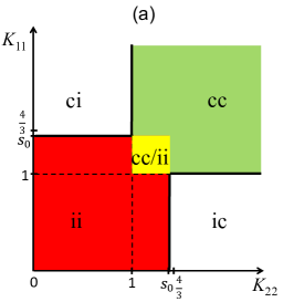
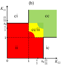
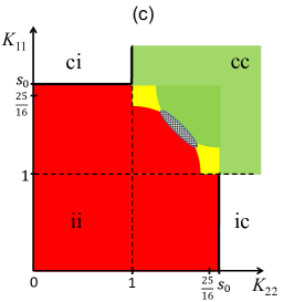
Figure 1: Schematic phase diagrams: (a) Under condition (30), when the one-particle scattering is dominant for all $K_{11}$ and $K_{22}$, the ${\mathrm{cc}}$ and ${\mathrm{ii}}$ phases are both stable with respect to one-particle scattering from a WS or a WL, respectively, in the square $1<K_{11},\,K_{22}<s_{0}$.  (b) With the inter-channel interaction increasing, the square of the ${\mathrm{cc}}$ - ${\mathrm{ii}}$ phase coexistence grows; however, for $s_{0}>\frac{4}{3}$ the ${\mathrm{cc}}$ (or ${\mathrm{ii}}$) phase becomes unstable with respect to two-particle scattering from a WS (or WL) in the lower (upper) corner of this square. (c) With further increase of $K_{12}$, at $|\cos\gamma|>3/5$, the two-particle scattering results in the appearance of the cross-hatched region on the phase diagram where both the ${\mathrm{ii}}$ and ${\mathrm{cc}}$ phases are unstable.

When scattering is possible in both channels, a more complicated picture emerges. To analyze which scattering configuration is RG dominant we represent ${\mathsf{K}}$ as a Gram matrix built of two vectors, $\{{K_{ij}}\}=\bm{g}_{i}\cdot\bm{g}_{j}$, where $|{\bm{g}}_{i}|=\sqrt{K_{ii}}$, while the angle $\gamma=\widehat{{\bm{g}}_{1}{\bm{g}}_{2}}$ is given by

$$\cos\gamma=\frac{K_{12}}{\sqrt{K_{11}K_{22}}}$$ (29)

Such a representation is possible when the inter-channel interaction is not too strong: for $K_{12}\geqslant\sqrt{K_{11}K_{22}}$ one enters the region of the Wentzel–Bardeen instability KLY (b) where the channels should be totally restructured. In the subsequent analysis we will stay clear of this region. In this representation $\Delta_{\mathrm{cc}}={\bm{G}}^{2}$ where ${\bm{G}}=n_{1}{\bm{g}}_{1}+n_{2}{\bm{g}}_{2},$ and a similar expression holds for $\Delta_{{\mathrm{ii}}}$ in terms of the inverse Luttinger matrix. Then the problem of finding a configuration corresponding to the most RG relevant scattering (which has the smallest $\Delta_{\mathrm{conf}}$) is reduced to that of finding the shortest vector on a $2D$ lattice spanned by ${\bm{g}}_{1}$ and ${\bm{g}}_{2}$. In general, this shortest vector problem (SVP) does not have an analytic solution and is known to be computationally hard Arora et al. (1997); *SVP. It is, however, possible to formulate the parametric conditions for which one-particle scattering, $n_{1}=1,\,n_{2}=0$ or $n_{1}=0,\,n_{2}=1$, dominates the RG flows KLY (a). It is shown in Appendix B that the sufficient condition for one-particle scattering to dominate is

$$K_{12}<\tfrac{1}{2}\min\{{K_{11},\,K_{22}}\}\quad\Leftrightarrow\quad|\cos\gamma|<\tfrac{1}{2}.$$ (30)

As $K_{12}$ is proportional to the inter-channel interaction strength, the above inequality holds when this interaction is sufficiently small.

To determine the boundaries between nontrivial phases in this case, we substitute $|n_{1}|=1,\,n_{2}=0$ or $n_{1}=0$, $|n_{2}|=1$ into the stability conditions of (28). Expressing $\kappa\equiv\det{\mathsf{K}}$ in terms of $\gamma$ as $\kappa=K_{11}K_{22}\sin^{2}\gamma$, we represent these conditions (with $s_{0}\equiv 1/{\sin^{2}\gamma}$) as

$$\begin{aligned} K_{11},\,K_{22}&>1\;\;({\mathrm{cc}});&K_{11},\,K_{22}&<s_{0}&&(\mathrm{ii});\\ \!\!\!K_{11}<1,\,K_{22}&>s_{0}\;({\mathrm{ic}});&K_{22}<1,\,K_{11}&>s_{0}&&(\mathrm{ci}).\end{aligned}$$ (31)

Since $s_{0}>1$ the boundaries of the cc and ii phases inevitably overlap, as illustrated in Fig. 1(a): inside the central square, i.e. for $1<K_{11},\,K_{22}<1/\sin^{2}\gamma$, the phase where both channels are conducting is stable against weak scattering while the phase where both are insulating is stable against weak tunneling. As the elements of ${\mathsf{K}}$ are the same for both phases, they can be only distinguished by the impurity scattering strength implicit in (19). Therefore, a new unstable fixed point characterized by some critical value of scattering should exist for any given ${\mathsf{K}}$. Such a scattering-dependent fixed point describes a transition between insulating and conducting phases simultaneous for both channels. Any transition between the ${\mathrm{c}}$ and ${\mathrm{i}}$ phases that happens only in one of the channels is fully defined by the parameters of the Lagrangian in (4) independently of the scattering strength. This is illustrated by the solid phase boundaries between ${\mathrm{ii}}$ and ${\mathrm{ic}}$ phases, etc., in Fig. 1.

When the inequality in (30) fails with increasing $K_{12}$, (29), which characterizes the inter-channel interaction, the one-particle scattering still dominates in certain parts of the phase diagram; the appropriate necessary conditions are derived in Appendix B. However, many-particle (first of all, two-particle) scattering starts to change the phase diagram. Note that the change affects only the ${\mathrm{cc}}$ and ${\mathrm{ii}}$ phases while the stability of the ${\mathrm{ic}}$ or ${\mathrm{ci}}$ phases is unaffected by the many-particle scattering, as seen from Eq. (28c,d).

We consider the most relevant case KLY (a) of the stability conditions, Eq. (28a,b), broken by the two-particle scattering. Substituting $|n_{1,2}|=1$ into (28a) and (28b) we find the two-particle instability conditions as follows:

$$\begin{aligned} \!\!\!\!K_{11}\pm 2\sqrt{K_{11}K_{22}}\cos\gamma\!+\!K_{22}&<1;&(\mathrm{cc})&\\ \!\!\!\!K_{11}\pm 2\sqrt{K_{11}K_{22}}\cos\gamma\!+\!K_{22}&<K_{11}K_{22}\sin^{2}\gamma.\!\!\!\!&(\mathrm{ii})&\end{aligned}$$ (32)

When $|\cos\gamma|>\frac{1}{2}$ (i.e. $s_{0}>\frac{4}{3}$), both these inequalities hold inside the parametric region of (31), where the $\mathrm{ii}$ and $\mathrm{cc}$ phases are stable with respect to the one-particle scattering. Thus going beyond the one-particle stability condition, (30), results in a more complicated form of the region of the phase coexistence as schematically illustrated in Fig. 1(b). There the yellow square, corresponding to the region of simultaneous stability of the $\mathrm{ii}$ and $\mathrm{cc}$ phases with respect to the one-particle scattering, increases; however, both these phases become unstable with respect to two-particle scattering in the corners of this square. The exact shape of the phase boundaries is not relevant but can be easily found from (32).

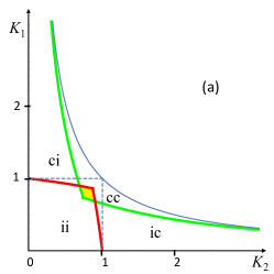
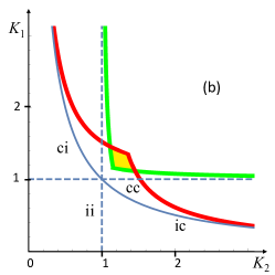
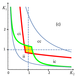
Figure 2: Phase diagrams for $\beta=1$ and different values of the inter-channel interaction parameters: (a) ${\widetilde{g}}_{4}=\widetilde{g}_{2}=0.5\,$; (b) $\widetilde{g}_{4}=-\widetilde{g}_{2}=0.5\,$; (c) $\widetilde{g}_{4}=0;\;\widetilde{g}_{2}=0.6\,$. The blue curves on each graph show the boundary of the Wentzel – Bardeen instability region, KLY (b) while in the yellow region both ${\mathrm{ii}}$ and ${\mathrm{cc}}$ phases are stable with respect to one-particle scattering. Here we assume that the condition of (30) is fulfilled, i.e. multiple scattering is irrelevant.

With further increase of the inter-channel interaction, (29), the regions of the two-particle instability start to overlap when both the inequalities in (32) hold simultaneously, see Fig. 1(c). This first happens in the center of the phase coexistence region, where $K_{11}=K_{22}$ which gives $|\cos\gamma|=\frac{3}{5}$ (i.e. $s_{0}=\frac{25}{16}$). Thus a totally new situation might emerge KLY (d) for $|\cos\gamma|>\frac{3}{5}$ where the ${\mathrm{cc}}$ phase is unstable against weak scattering, while the ${\mathrm{ii}}$ phase is unstable against a weak link. This signals the existence of a non-trivial attractive fixed point at some intermediate value of the scattering strength. Again, the RG flows in its vicinity depend on the impurity scattering strength. The conductance of each channel in such a case is finite, but smaller than the ideal value. It might be possible in such a case to redefine the channels so that one of them would become fully insulating while the other ideally conducting, as we illustrate in Section V.

IV.2 Scattering boundaries in two-channel LL

The elements of the Luttinger matrix that define the phase stability conditions and thus the boundaries of all the phases are implicitly dependent on the inter-channel interaction strengths, $V_{\theta,\varphi}$, as well as on the particle velocities, $v_{1,2}$, and the Luttinger parameters, $K_{1,2}$, in both the channels. Here we explicitly derive this dependence.

The $2\times 2$ Luttinger matrix ${\mathsf{K}}$, which governs the stability conditions (28), is defined via the interaction matrices, ${\mathsf{V}}_{\theta}$ and ${\mathsf{V}}_{\varphi}$, by (10). Now we will express ${\mathsf{K}}$ explicitly in terms of matrix elements of ${\mathsf{V}}_{\theta,\varphi}$. In the two-channel case these matrices, which define the Lagrangian (4), are represented in terms of the inter-channel density-density and current-current interaction strengths, $V_{\varphi}$ and $V_{\theta}$, the Luttinger parameters, $K_{1,2}$, and renormalized velocities, $v_{1,2}$, in each channel as follows:

$${\mathsf{V}}_{\theta} =\begin{pmatrix}v_{1}K_{1}^{-1}&V_{\theta}\\ V_{\theta}&v_{2}K_{2}^{-1}\\ \end{pmatrix}, {\mathsf{V}}_{\varphi} =\begin{pmatrix}v_{1}K_{1}&V_{\varphi}\\ V_{\varphi}&v_{2}K_{2}\\ \end{pmatrix}.$$ (33)

Using the fact that the determinants of ${\mathsf{V}}_{{\theta,\varphi}}$ are positive KLY (b), we represent them as

$$\det{\mathsf{V}}_{\theta} =\frac{v_{1}v_{2}\cos^{2}\alpha_{\theta}}{K_{1}K_{2}}, \det{\mathsf{V}}_{\varphi} ={v_{1}v_{2}K_{1}K_{2}}\cos^{2}\alpha_{\varphi},$$ (34a)

where

$$\begin{aligned} \sin\alpha_{\theta}&\equiv\sqrt{\frac{K_{1}K_{2}}{v_{1}v_{2}}}V_{\theta}\equiv\sqrt{K_{1}K_{2}}({\widetilde{g}_{4}+\widetilde{g}_{2}}),\\ \sin\alpha_{\varphi}&\equiv\frac{V_{\varphi}}{\sqrt{K_{1}K_{2}}}\equiv\frac{{\widetilde{g}_{4}-\widetilde{g}_{2}}}{\sqrt{K_{1}K_{2}}},\end{aligned}$$ (34b)

and $\widetilde{g}_{4,2}$ characterize inter-channel interactions of the density components of the same or opposite chirality. Substituting this into (14), with ${\mathsf{A}}\equiv{\mathsf{V}}_{\theta}$ and ${\mathsf{B}}\equiv{\mathsf{V}}_{\varphi}$, we arrive at the following representation of the Luttinger matrix:

$${\mathsf{K}} =\frac{1}{B}\begin{pmatrix}K_{1}(\beta+\rho)&{\frac{\sqrt{\beta K_{1}K_{2}}\sin({\alpha_{\varphi}-\alpha_{\theta}})}{\cos\alpha_{\theta}}}\\[6.0pt] {\frac{\sqrt{\beta K_{1}K_{2}}\sin({\alpha_{\varphi}-\alpha_{\theta}})}{\cos\alpha_{\theta}}}&K_{2}({1+\beta\rho})\end{pmatrix}$$

$$=\begin{pmatrix}{K_{1}}/{K_{{\mathrm{c}}1}}&K_{12}\\[6.0pt] K_{12}&{K_{2}}/{K_{{\mathrm{c}}2}}\\ \end{pmatrix},\quad\begin{array}[]{lcl}K_{\mathrm{c}1}&\equiv&\frac{B}{\beta+\rho}\\[6.0pt] K_{\mathrm{c}2}&\equiv&\frac{B}{1+\beta\rho}\end{array}$$ (37)

where $B\equiv\sqrt{1+\beta^{2}+2\beta\cos({\alpha_{\varphi}-\alpha_{\theta}})},$ $\beta\equiv{v_{1}}/{v_{2}},$ and $\rho\equiv{\cos\alpha_{\varphi}}/{\cos\alpha_{\theta}}.$

To express the phase boundaries in Fig. 1 in these terms, we note that $\kappa\equiv\det{\mathsf{K}}=K_{1}K_{2}|\rho|$ as follows from (10) and (34). On the other hand, $\kappa=K_{11}K_{22}\sin^{2}\gamma$. Therefore, substituting $1/s_{0}\equiv\sin^{2}\gamma=\rho K_{{\mathrm{c1}}}K_{\mathrm{c2}}$ in (31) we find

$$\begin{aligned} K_{1}&>K_{{\mathrm{c}}1}\cr K_{2}&>K_{\mathrm{c}2}\end{aligned}{\mathrm{(cc)}} \begin{aligned} K_{1}&<1/\rho{K_{{\mathrm{c}}2}};\cr K_{2}&<1/\rho{K_{{\mathrm{c}}1}}\end{aligned}{\mathrm{(ii)}}.$$ (38)

Thus the phase diagram with allowance only for the one-particle scattering looks on the $K_{1}$ - $K_{2}$ plane exactly as that in Fig. 1(a) with the straight boundaries being defined by the inequalities (38).

However, such a picture is deceptively simple: both $K_{{\mathrm{c}}1}$ and $K_{{\mathrm{c}}2}$ nontrivially depend on the five parameters in (37) that define the clean two-channel Luttinger liquid: the Luttinger parameters in each channel themselves, the velocity ratio, and the two inter-channel interaction parameters. We illustrate such a dependence by fixing the values of some of these parameters. Choosing $v_{1}=v_{2}\equiv v$ simplifies the expressions for the boundaries: it follows from (37) that $K_{\mathrm{c}}\equiv K_{\mathrm{c1}}=K_{\mathrm{c2}}=\cos\alpha_{\theta}/\cos\frac{1}{2}({\alpha_{\theta}+\alpha_{\varphi}})$ and $1/\rho K_{\mathrm{c}}=\cos\frac{1}{2}({\alpha_{\theta}+\alpha_{\varphi}})/\cos\alpha_{\varphi}$. Specifying three different choices of the inter-channel interaction in (34) via $\widetilde{g}_{4,2}$, with $V_{\theta,\varphi}\equiv v({\widetilde{g}_{4}\pm\widetilde{g}_{2}})$, we arrive at three examples in Fig. 2. Note that, although we have chosen $\beta=1$ for illustrations, there is an important robust feature on these phase diagram: for any $\beta$ the yellow region, representing the $\mathrm{cc}$-$\mathrm{ii}$ phase coexistence, is always below the lines $K_{1,2}=1$ for $\alpha_{\theta}>\alpha_{\varphi}>0$ (a), or above these lines for $\alpha_{\varphi}>\alpha_{\theta}>0$ (b), while the noninteracting point $K_{1}=K_{2}=1$ is inside these region when the signs of the inter-channel interaction parameters $\alpha_{\theta,\varphi}$ are opposite (c). We do not show in Fig. 2 the boundaries of two-particle instability, which is analytically obtained in Appendix B by substituting elements of matrix ${\mathsf{K}}$, (37), into condition (32).

V Weak scatterer and weak link in two-channel topological insulators

Now let us consider in more detail another example of a two-channel LL: a 2D topological insulator supporting two helical states at each edge Hou et al. (2009); Santos and Gutman (2015). We analyze whether current-carrying edge states remain stable against potential scattering as in (19). The time-reversal symmetry forbids intra-edge scattering, while a spin-conserving backscattering between the edges is allowed. The scattering amplitude can be regulated by a distance between the edge states and can be locally increased when they approach each other, e.g., like in quantum point contacts (QPC) in a narrow Hall bar geometry Choi et al. (2015). Assuming that both these channels are of the same physical nature so that $K_{1}=K_{2}\equiv K$ and $\beta\equiv v_{1}/v_{2}=1$, it is convenient to form the initial channels from spin-up and spin-down electrons so that left- and right-movers in each channel belong to the opposite edge. The backscattering then becomes an intra-channel process while the inter-channel scattering is forbidden by time-reversal symmetry.

With such a choice of the channels, the present case falls within the generic analysis of the previous sections. The two-channel Luttinger matrix (37) simplifies:

$${\mathsf{K}} =\dfrac{K{\mathrm{sgn}[\cos\frac{\alpha_{\varphi}-\alpha_{\theta}}{2}]}}{\cos\alpha_{\theta}}\begin{pmatrix}\cos\frac{\alpha_{\varphi}+\alpha_{\theta}}{2}&\sin\frac{\alpha_{\varphi}-\alpha_{\theta}}{2}\\[4.0pt] \sin\frac{\alpha_{\varphi}-\alpha_{\theta}}{2}&\cos\frac{\alpha_{\varphi}+\alpha_{\theta}}{2}\\ \end{pmatrix}.$$ (39)

Note that in this case the mixed ${\mathrm{ci/ic}}$ phases are inevitably unstable against one-particle scattering as the diagonal elements of the Luttinger matrix above are equal to each other thus violating the stability conditions for these phases in (31).

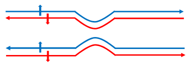
Figure 3: Helical edge currents in a topological insulator with QPC. We re-label the channels so that spin-up electrons at the opposite edges form one channel and spin-down the other. In this nomenclature, only a local intra-channel scattering is allowed at the QPC since the inter-channel one is forbidden by the time-reversal symmetry. On the other hand, the interaction between the modes of opposite helicity at each edge is translated into the inter-channel interaction while the intra-channel one is suppressed due to a spatial separation between the modes belonging to the same channel.

It is reasonable to assume that only particles at the same edge are interacting (apart from relatively short regions of QPC where the interaction can be absorbed into the scattering coefficients). Then the inter-channel interaction is always between the particles of the opposite chirality, $\widetilde{g}_{4}=0$, i.e. $V_{\theta}=-V_{\varphi}$ in (34) resulting in $\sin\alpha_{\varphi}=-\sin\alpha_{\theta}/K^{2}$ so that the Luttinger matrix (39) depends only on two parameters. In a particular case of the channels in Fig. 3 built from the interacting electrons, the intra-channel interaction contains only $g_{4}$-proportional term resulting Giamarchi (2004) in $K=1$. In this case from $V_{\theta}=-V_{\varphi}$ follows $\alpha_{\theta}=-\alpha_{\varphi}\equiv\alpha$ so that (39) reduces to

$${\mathsf{K}} =\frac{1}{|\cos\alpha|}\begin{pmatrix}1&-\sin\alpha\\ -\sin\alpha&1\\ \end{pmatrix}.$$ (40)

Graphically, this state corresponds to the middle point, $K_{1}=K_{2}=1$, in the phase diagram (c) in Fig. 2 which lies in the ${\mathrm{ii}}$ – ${\mathrm{cc}}$ phase coexistence region where both these phases are stable with respect to one-particle scattering. There the ultimate choice of the phase depends on the impurity scattering strength. Thus, although the ${\mathrm{cc}}$ state is protected against weak scattering, as has been noted earlier Santos and Gutman (2015), no protection against strong scattering exists.

Even such a limited ‘protection’ fails with increasing the inter-channel interaction so that two-particle scattering becomes relevant. This happens at $|\sin\alpha|\geqslant\frac{3}{5}$ after the two instability regions meet at the center, $K_{1}=K_{2}=1$, in Fig. 1(c). To prove this, it is worth rewriting the RG exponents for the ${\mathrm{ii}}$ and ${\mathrm{cc}}$ phases, (28), for the present case:

$$\Delta_{{\mathrm{cc}/\mathrm{ii}}}=\frac{n_{\uparrow}^{2}+n_{\downarrow}^{2}\mp 2n_{\uparrow}n_{\downarrow}\sin\alpha}{|\cos\alpha|}.$$ (41)

For the two-particle scattering, $|n_{\uparrow}|=|n_{\downarrow}|=1$, these exponents are smaller than $1$ (making the phases unstable) for $|\sin\alpha|>\frac{3}{5}$. Naturally, this condition is equivalent to the general one, $|\cos\gamma|>\frac{3}{5}$, Fig. 1(c), as it follows from the definition of $\gamma$, (29), that $\cos\gamma=-\sin\alpha$ for the matrix (40). Under this condition there should exist, as described earlier, an intermediate stable fixed point corresponding to finite conductance of both the spin-up and spin-down channel.

Such a finite conductance, however, usually signifies the possibility of introducing composite channels, one continuous (ideal conductance) and one split (no conductance). In the present case, they correspond to the standard ‘charge-spin separation’ choice of channels. Indeed, introducing $n_{\mathrm{ch}}=n_{\uparrow}+n_{\downarrow}$ and $n_{\mathrm{sp}}=n_{\uparrow}-n_{\downarrow}$ diagonalizes (41) for the RG exponents: $\Delta_{\mathrm{cc}}=\frac{1}{2}(K_{\mathrm{ch}}n_{\mathrm{ch}}^{2}+K_{\mathrm{sp}}n_{\mathrm{sp}}^{2})$ and $\Delta_{\mathrm{ii}}=\frac{1}{2}(K_{\mathrm{ch}}^{-1}n_{\mathrm{ch}}^{2}+K_{\mathrm{sp}}^{-1}n_{\mathrm{sp}}^{2})$ where $K_{\mathrm{ch}}=K_{\mathrm{sp}}^{-1}=({1-\sin\alpha})/|\cos\alpha|$. As $n_{\mathrm{ch}}+n_{\mathrm{sp}}$ must be even, the lowest order scattering process is $|n_{\mathrm{ch}}|=|n_{\mathrm{sp}}|=1$, corresponding to the (RG irrelevant) one-particle scattering in the ‘old’ spin-up and spin-down channels. For such a process $\Delta_{\mathrm{cc}}=\Delta_{\mathrm{ii}}=\frac{1}{2}({K_{\mathrm{ch}}+K_{\mathrm{ch}}^{-1}})=1/|\cos\alpha|>1$.

The lowest-order charge-only ($|n_{\mathrm{ch}}|=2$) or spin-only ($|n_{\mathrm{sp}}|=2$) scattering processes correspond to the two-particle scattering in the ‘old’ channels with $n_{\uparrow}=n_{\downarrow}=\pm 1$ or $n_{\uparrow}=-n_{\downarrow}=\pm 1$, respectively. Thus, although both the ${\mathrm{cc}}$ and ${\mathrm{ii}}$ phases are unstable with respect to the two-particle scattering for $|\sin\alpha|>\frac{3}{5}$, the instability reveals itself in different ways depending on the sign of $\alpha$. For the repulsive inter-channel interaction ($\alpha>0$), the charge channel becomes insulating while the spin one remains ideally conducting, while for the attractive interaction ( $\alpha<0$) the roles of the charge and spin channels are inverted. For the weak or intermediate inter-channel interaction, $|\sin\alpha|<\frac{3}{5}$, both new channels remain conducting so that both ${\mathrm{cc}}$ and ${\mathrm{ii}}$ phases remain stable, corresponding to the existence of an unstable fixed point with RG flows depending on the scattering strength.

Any two-channel LL with the intra-channel interaction and inter-channel scattering suppressed fits into the scenario described in this section. In particular, it reproduces the earlier result Hou et al. (2009) on a corner junction between the edge currents in topological insulators. Let us also repeat that the idea of ‘interaction-protected’ transport verified for weak scattering Santos and Gutman (2015) needs analysis also for strong scattering (weak links). The results of this section show that for any intra-level interaction the edge currents are only stable against weak scattering, while allowing for two-particle scattering in the presence of a sufficiently strong intra-level interaction completely suppresses the edge currents.

VI Conclusion

We have developed a powerful approach to deal with a local impurity in multichannel Luttinger liquids. We have identified the Luttinger matrix, (9), (10) and (37), that controls scaling dimensions of all perturbations in all possible phases. Thus we have obtained the phase diagram for a generic two-channel Luttinger liquid, Fig. 1, that in certain parametric regions is governed by multiple scattering from the impurity KLY (a). We have constructed the phase boundaries that depend on the strength of inter-channel interaction as well as on the intra-channel LL characteristics, Fig. 2. The presented approach is applicable to channels of different nature as in fermion-boson mixtures, or to identical ones as on the opposite edges of a topological insulator. In the future we will extend it to particular interesting cases of a multi-channel LL.

Appendix A Scaling dimensions

As the Lagrangian in terms of the fields $\widetilde{{\bm{\theta}}}$ and $\widetilde{{\bm{\varphi}}}$, (15) and (16), is diagonal, the correlation functions are standard. Incorporating the boundary conditions, (23), results Yurkevich (2013); *YY2014 in the $\widetilde{\theta}$-$\widetilde{\theta}$ and $\widetilde{\varphi}$-$\widetilde{\varphi}$ correlations of (25), and the following antisymmetric correlations of $\widetilde{{\bm{\theta}}}$ and $\widetilde{{\bm{\varphi}}}$:

$$-\langle\Delta{\widetilde{\bm{\varphi}}}(t)\otimes 2{\widetilde{\bm{\theta}}}^{\rm T}\!(t^{\prime})\rangle =\langle{2\widetilde{\bm{\theta}}}(t)\otimes\Delta{\widetilde{\bm{\varphi}}}^{\rm T}\!(t^{\prime})\rangle=({\widetilde{\mathsf{R}}}-{\widetilde{\mathsf{T}}})\ell$$ (42)

with $\ell\equiv\ln(t-t^{\prime})$. This results after rotation (8) in the correlations of the original fields ${{\bm{\theta}}}$ and ${{\bm{\varphi}}}$ given in (26) and their cross-correlation given below:

$$\langle{\bm{\theta}}(t)\otimes\Delta{\bm{\varphi}}^{\rm T}\!({t^{\prime}})\rangle =\phantom{-}\frac{\Xi{\mathsf{K}}}{1+\Xi{\mathsf{K}}}\ell\,,$$ (43)

$$\langle{\Delta{\bm{\varphi}}\otimes\bm{\theta}}(t)^{\rm T}\!({t^{\prime}})\rangle =-\frac{{\mathsf{K}}\Xi}{1+{\mathsf{K}}\Xi}\ell\,.$$ (44)

The above structure guarantees that the cross-correlations will not affect correlation functions of linear combinations of the type ${\bm{a\cdot\theta}}+{\bm{b\cdot}}\Delta{\bm{\varphi}}$, and thus will not enter the RG dimensions calculated below.

In the physical limit described after (18) the boundary conditions for ${\bm{\theta}}$ are relevant in continuous channels and for ${\bm{\varphi}}$ in split channels. To take the limit, we relabel the channels so that the first $n$ are continuous and the rest $N-n$ are split. In such a basis the Luttinger matrix and its inverse can be written as

while $\Xi\equiv\operatorname{diag}(\hat{\xi}_{\mathrm{c}},\hat{\xi}_{\mathrm{i}})$ where in the physical limit all the elements of the diagonal $n\times n$ matrix $\hat{\xi}_{\mathrm{c}}$ go to zero, and all the elements of the diagonal $(N-n)\times({N-n})$ matrix $\hat{\xi}_{\mathrm{i}}$ to infinity. Obviously, $\overline{{\mathsf{K}}}_{\mathrm{cc}}\neq{{\mathsf{K}}}_{\mathrm{cc}}^{-1}$, as the elements of the former matrix depend on all the elements of matrix ${\mathsf{K}}$. In these notations one finds that

$$\begin{aligned} \lim_{\xi}\left[{\mathsf{K}}^{-1}+\Xi\right]^{-1}&=\left(\begin{array}[]{cc}\overline{{\mathsf{K}}}_{\mathrm{cc}}^{\,\,-1}&0\\ 0&0\\ \end{array}\right)\,,\\ \lim_{\xi}\left[{\mathsf{K}}+\Xi^{-1}\right]^{-1}&=\left(\begin{array}[]{cc}0&0\\ 0&{{\mathsf{K}}}_{\mathrm{ii}}^{\,-1}\\ \end{array}\right)\,.\end{aligned}$$ (45)

Thus in terms of the relabeled channels the right-hand sides of (26a) and (26b) go over to $\overline{{\mathsf{K}}}_{\mathrm{cc}}^{\,\,-1}\ell$ and ${{\mathsf{K}}}_{\mathrm{ii}}^{\,-1}\ell$, respectively.

Using the relabeled channels, we rewrite the Lagrangian density of (19) as

$${\cal L}_{\rm sc} =\sum_{{\bm{n}}}v_{\bm{n}}\,e^{i{\bm{n}}\cdot{\bm{\Phi}}}+\mathrm{c.c.}\,, {\bm{\Phi}} =\begin{pmatrix}2{\bm{\theta}}\\ \Delta{\bm{\varphi}}\\ \end{pmatrix}, {\bm{n}} =\begin{pmatrix}{\bm{n}}_{c}\\ {\bm{n}}_{i}\\ \end{pmatrix}\,,$$ (46)

where ${\bm{n}}_{c}$ and ${\bm{n}}_{i}$ are integer-valued vectors belonging to the ${\mathrm{c}}$- and ${\mathrm{i}}$-subspaces, respectively, that describe the multiplicity of backscattering in the former and of tunneling in the latter. The correlation function of fields ${\bm{\Phi}}$ is not contributed by the the off-diagonal correlation of (43) and is obtained from (26) in the limit (45) as follows:

$$\tfrac{1}{2}\,\langle{\bm{\Phi}}(t)\otimes{\bm{\Phi}}^{\rm T}\!({t^{\prime}})\rangle=\begin{pmatrix}\overline{{\mathsf{K}}}_{\mathrm{cc}}^{\,\,-1}&0\\ 0&{\mathsf{K}}_{{\mathrm{ii}}}^{-1}\\ \end{pmatrix}=\begin{pmatrix}\overline{{\mathsf{K}}}_{\mathrm{cc}}^{\phantom{-1}}\!\!\!\!&0\\ 0&{\mathsf{K}}_{{\mathrm{ii}}}^{\phantom{-1}}\!\!\!\!\\ \end{pmatrix}^{-1}\!\!\!\!.$$ (47)

Therefore, the scaling dimension of each term in Lagrangian (46) can be written as

$${\mathrm{dim}}\left[v_{\bm{n}}\,e^{i{\bm{n}}^{\rm T}{\bm{\Phi}}}\right]={\bm{n}}^{\rm T}\left(\begin{array}[]{cc}{\bar{\mathsf{K}}}_{\rm cc}&0\\ 0&{\mathsf{K}}_{\rm ii}\\ \end{array}\right)^{-1}{\bm{n}}\,.$$ (50)

Now we use the projector operators of (22) to restore the original numbering of the channels which gives

$${\overline{{\mathsf{K}}}}_{\rm cc} \to{\mathsf{P}}_{\rm c}\,{\mathsf{K}}^{-1}\,{\mathsf{P}}_{\rm c}\,, {\mathsf{K}}_{\rm ii} \to{\mathsf{P}}_{\rm i}\,{\mathsf{K}}\,{\mathsf{P}}_{\rm i}\,,$$ (51)

Combining this with (50) results in (27) in the main text.

Appendix B the shortest vector problem

Finding the minimum of a quadratic form built on integer-valued vectors is equivalent to finding the shortest vector connecting nodes on a lattice. Although this problem in its completeness is known to be computationally hard Arora et al. (1997); *SVP determining the sufficient condition for the shortest vector to be not an elementary lattice vector is straightforward. This is all we need to define the parametric region in which one-particle scattering is not necessarily RG-dominant.

The elements of the $2\times 2$ Luttinger matrix ${\mathsf{K}}$ in the Gram representation are written as $\{{K_{ij}}\}=\bm{g}_{i}\cdot\bm{g}_{j}$, where $|{\bm{g}}_{i}|=\sqrt{K_{ii}}$, while the angle $\gamma=\widehat{{\bm{g}}_{1}{\bm{g}}_{2}}$ is given by (29). Then one has to find the minimum of $|\bm{G}|^{2}$ where ${\bm{G}}=n_{1}{\bm{g}}_{1}+n_{2}{\bm{g}}_{2}$, i.e. the minimal distance between two nodes on a two-dimensional lattice spanned by the basis vectors ${\bm{g}}_{1,2}$. For a rectangular lattice ($\cos\gamma=0$) the solution is the shortest lattice spacing, corresponding to $n_{1}=0\,,\,n_{2}=\pm 1$ (assuming $g_{1}>g_{2}$).

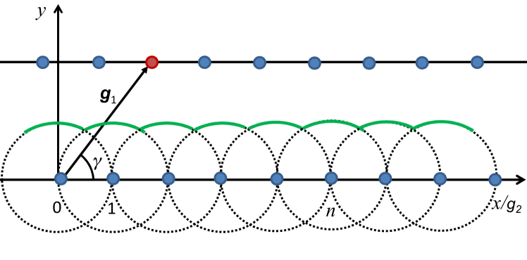
Figure 4: The SVP illustration. With $\gamma$ decreasing, the nearest horizontal chains of the lattice become closer. At some critical angle, the upper chain crosses the boundary made by circles of radius $g_{2}$ around each node of the lower chain. Then the shortest distance between the nodes of the upper and lower chains is less than the length of the shortest basis vector $\bm{g}_{2}$.

On decreasing the lattice angle $\gamma$ with $g_{1}\geqslant g_{2}$ being constant, the horizontal lattice chains become closer as illustrated in Fig. 4. We draw there the circles of radius $g_{2}$ centered at the lattice nodes on the low horizontal chain (with $y=0$). Measuring all lengths in units of $g_{2}$, the $y$ coordinate of the upper boundary of these circles can be written as $y=\sqrt{1-\{{R\cos\gamma}\}^{2}}$, where $R\equiv g_{1}/g_{2}\geqslant 1$ and $\{{A}\}$ is the distance of $A$ to the closest integer $n$ (so that $-\frac{1}{2}\leqslant\{{A}\}\leqslant\frac{1}{2}$). When the end of basis vector $\bm{g}_{1}$ touches this boundary, the distance between the zeroth node of the upper and the $n^{{\mathrm{th}}}$ node of the lower chains equals $g_{2}$ and becomes smaller with $\gamma$ further decreasing – this is where the $n$-particle scattering becomes more RG-relevant than the one-particle. As the $x$ coordinate of $\bm{g}_{1}$ equals $R\sin\gamma$, the condition for this not to happen for any $n$ is

$$R^{2}\sin^{2}\gamma+\{R\cos\gamma\}^{2}>1\,,$$ (52)

Since $R\equiv g_{1}/g_{2}\geqslant 1$ and $\{R\cos\gamma\}^{2}\leqslant\frac{1}{4}$, the inequality is satisfied for any $R$ when $\cos\gamma<\frac{1}{2}$. When the inequality fails, the multiplicity $n$ of the scattering process which is more RG relevant than one-particle scattering is given by $n=\left[R\cos\gamma\right]+1$ where $\left[A\right]$ is an integer closest to $A$. Thus, depending on the ratio $R$, it could arbitrary large. For the important case of $R=1$ (considered in Section V), it is the physically relevant KLY (a) two-particle scattering that becomes more RG relevant than one-particle for $\cos\gamma<\frac{1}{2}$.

References

- Teo and Kane (2014) Jeffrey C Y Teo and C L Kane, “From Luttinger liquid to non-Abelian quantum Hall states,” Phys. Rev. B 89, 085101 (2014).
- Sondhi and Yang (2001) S. L. Sondhi and Kun Yang, “Sliding phases via magnetic fields,” Phys. Rev. B 63, 054430 (2001).
- Kane et al. (2002) C L Kane, R Mukhopadhyay, and T C Lubensky, “Fractional quantum Hall effect in an array of quantum wires,” Phys. Rev. Lett. 88, 036401 (2002).
- O’Hern et al. (1999) C. S. O’Hern, T. C. Lubensky, and J. Toner, “Sliding phases in models, crystals, and cationic lipid-DNA complexes,” Phys. Rev. Lett. 83, 2745–2748 (1999).
- Vishwanath and Carpentier (2001) Ashvin Vishwanath and David Carpentier, “Two-dimensional anisotropic non-Fermi-liquid phase of coupled Luttinger liquids,” Phys. Rev. Lett. 86, 676–679 (2001).
- Mukhopadhyay et al. (2001) Ranjan Mukhopadhyay, C. L. Kane, and T. C. Lubensky, “Crossed sliding Luttinger liquid phase,” Phys. Rev. B 63, 081103 (2001).
- Cazalilla and Ho (2003) M. A. Cazalilla and A. F. Ho, “Instabilities in binary mixtures of one-dimensional quantum degenerate gases,” Phys. Rev. Lett. 91, 150403 (2003).
- Mathey et al. (2004) L. Mathey, D.-W. Wang, W. Hofstetter, M. D. Lukin, and Eugene Demler, “Luttinger liquid of polarons in one-dimensional boson-fermion mixtures,” Phys. Rev. Lett. 93, 120404 (2004).
- Crépin et al. (2010) F Crépin, Gergely Zaránd, and Pascal Simon, “Disordered one-dimensional Bose-Fermi mixtures: The Bose-Fermi glass,” Phys. Rev. Lett. 105, 115301 (2010).
- Crépin et al. (2012) F Crépin, Gergely Zaránd, and Pascal Simon, “Mixtures of ultracold atoms in one-dimensional disordered potentials,” Phys. Rev. A 85, 023625 (2012).
- San-Jose et al. (2005) Pablo San-Jose, Francisco Guinea, and Thierry Martin, “Electron backscattering from dynamical impurities in a Luttinger liquid,” Phys. Rev. B 72, 165427 (2005).
- Galda et al. (2011a) Alexey Galda, Igor V. Yurkevich, and Igor V. Lerner, “Impurity scattering in a Luttinger liquid with electron-phonon coupling,” Phys. Rev. B 83, R041106 (2011a).
- Galda et al. (2011b) A. Galda, I. V. Yurkevich, and I. V. Lerner, “Effect of electron-phonon coupling on transmission through Luttinger liquid hybridized with resonant level,” EPL 93, 17009 (2011b).
- Yurkevich et al. (2013) Igor V. Yurkevich, Alexey Galda, Oleg M. Yevtushenko, and Igor V. Lerner, “Duality of weak and strong scatterer in a Luttinger liquid coupled to massless bosons,” Phys. Rev. Lett. 110, 136405 (2013).
- Yurkevich (2013) Igor V. Yurkevich, “Duality in multi-channel Luttinger liquid with local scatterer,” EPL 104, 37004 (2013).
- Yurkevich and Yevtushenko (2014) Igor V. Yurkevich and Oleg M. Yevtushenko, “Universal duality in a Luttinger liquid coupled to a generic environment,” Phys. Rev. B 90, 115411 (2014).
- Hou et al. (2009) Chang-Yu Hou, Eun-Ah Kim, and Claudio Chamon, “Corner junction as a probe of helical edge states,” Phys. Rev. Lett. 102, 076602 (2009).
- Santos and Gutman (2015) Raul A. Santos and D. B. Gutman, “Interaction-protected topological insulators with time reversal symmetry,” Phys. Rev. B 92, 075135 (2015).
- Kane and Fisher (1992a) C L Kane and M P A Fisher, “Transport in a one-channel Luttinger liquid,” Phys. Rev. Lett. 68, 1220 (1992a).
- Kane and Fisher (1992b) C L Kane and M P A Fisher, “Resonant tunneling in an interacting one-dimensional electron gas,” Phys. Rev. B 46, 7268(R) (1992b).
- Kane and Fisher (1992c) C. L. Kane and Matthew P. A. Fisher, “Transmission through barriers and resonant tunneling in an interacting one-dimensional electron gas,” Phys. Rev. B 46, 15233–15262 (1992c).
- Maslov and Stone (1995) D L Maslov and M Stone, “Landauer conductance of Luttinger liquids with leads,” Phys. Rev. B 52, R5539 (1995).
- Ponomarenko (1995) V. V. Ponomarenko, “Renormalization of the one-dimensional conductance in the Luttinger-liquid model,” Phys. Rev. B 52, R8666–R8667 (1995).
- Safi and Schulz (1995) I. Safi and H. J. Schulz, “Transport in an inhomogeneous interacting one-dimensional system,” Phys. Rev. B 52, R17040–R17043 (1995).
- Giamarchi and Schulz (1988) T. Giamarchi and H. J. Schulz, “Anderson localization and interactions in one-dimensional metals,” Phys. Rev. B 37, 325–340 (1988).
- Basko et al. (2006) D M Basko, I L Aleiner, and B L Altshuler, “Metal-insulator transition in a weakly interacting many-electron system with localized single-particle states,” Ann. Phys. 321, 1126 (2006).
- Basko et al. (2007) D. M. Basko, I. L. Aleiner, and B. L. Altshuler, “Possible experimental manifestations of the many-body localization,” Phys. Rev. B 76, 052203 (2007).
- Aleiner et al. (2010) I. L. Aleiner, B. L. Altshuler, and G. V. Shlyapnikov, “A finite-temperature phase transition for disordered weakly interacting bosons in one dimension,” Nature Phys. 6, 900 (2010).
- KLY (a) The most RG-relevant scattering corresponds to the configuration with the lowest scaling dimension, see Eq. (27). However, bare amplitudes of multiparticle scattering are proportional to the appropriate power of a small parameter so that the regime where the most relevant multipatricle scattering dominates might only be reached at very lowe temperatures.,.
- Haldane (1981) F D M Haldane, “Luttinger liquid theory of one-dimensional quantum fluids,” J. Phys. C 14, 2585 (1981).
- KLY (b) In the present case, both and must be positive to avoid instabilities of the Wentzel–Bardeen type originally found Wentzel (1951); *Bardeen:51 for the electron-phonon interaction in . .
- KLY (c) The cross-correlations of and are antisymmetric, see Appendix A, and thus do not contribute to RG flows of the scattering terms of Eq. (19).
- Arora et al. (1997) S Arora, L Babai, J Stern, and Z Sweedyk, “The hardness of approximate optima in lattices, codes, and systems of linear equations,” J Comput Syst Sci 54, 317 (1997).
- Micciancio (2014) D. Micciancio, “The shortest vector in a lattice is hard to approximate to within some constant,” SIAM J. Comput. 30, 2008 (2014).
- KLY (d) Such an instability can be due to an unreasonable original choice of the channels, e.g., electrons with opposite spins, when a WS suppresses charge current but has no impact on a spin current, leading to a finite conductivity of each original channel. However, a non-trivial situation emerges where the original choice is fixed by the boundary conditions on the leads, or spatial positions of the interacting channels, or different nature of them like in the fermion-boson case, etc.
- Choi et al. (2015) H. K. Choi, I. Sivan, A. Rosenblatt, M. Heiblum, V. Umansky, and D. Mahalu, “Robust electron pairing in the integer quantum hall effect regime,” Nat Commun 6, 7435 (2015).
- Giamarchi (2004) T Giamarchi, Quantum Physics in One Dimension (Clarendon Press, London, 2004).
- Wentzel (1951) Gregor Wentzel, “The interaction of lattice vibrations with electrons in a metal,” Phys. Rev. 83, 168–169 (1951).
- Bardeen (1951) J Bardeen, “Electron-vibration interactions and superconductivity,” Rev. Mod. Phys. 23, 261 (1951).