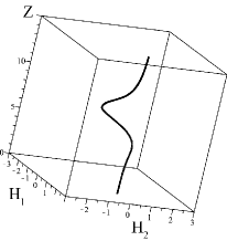
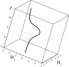
Nonlinear Dynamo

1,2M.I.Kopp, 3A.V.Tur 1,2V.V.Yanovsky
Abstract

In this manuscript using the asymptotic method of multiscale nonlinear theory we construct a nonlinear theory of the appearance of large-scale structures in the stratified conductive medium with the presence of small-scale oscillations of the velocity field and magnetic fields. These small-scale stationary oscillations are maintained by small external sources at low Reynolds numbers. We obtain a nonlinear system of equations describing the evolution of large-scale structures of the velocity field and magnetic fields. The linear stage of evolution leads to the known instability. In this article we consider the stationary large-scale structures of a magnetic field arising at stabilization of linear instability.

1Institute for Single Crystals, NAS Ukraine, Nauky Ave. 60, Kharkov 31001, Ukraine

2 V.N. Karazin Kharkiv National University 4 Svobody Sq., Kharkov 61022, Ukraine

3Universite de Toulouse [UPS], CNRS, Institut de Recherche en Astrophysique et Planetologie, 9 avenue du Colonel Roche, BP 44346, 31028 Toulouse Cedex 4, France


1 Introduction

It is known, that the term “dynamo” originated in theory of the generation of large-scale magnetic fields in magnetic hydrodynamics, mainly in its applications to astrophysics and geophysics. The main mechanism of the generation of large-scale magnetic fields (i.e., the dynamo mechanism) is a violation of the parity of fluid velocity field. In particular, a violation of parity leads to a non-zero velocity field helicity α=<VrotV>𝛼expectation𝑉𝑟𝑜𝑡𝑉\alpha=<\vec{V}rot\vec{V}> (α𝛼\alpha-effect). Here α is pseudo scalar . More generally, the violation of parity gives AKA effect (anisotropic kinetic α effect). In turn, these effects generate large-scale magnetic field instability and generate large-scale vortex instability of fluid. In recent years, this effect got the name of vortex dynamo. Currently the theory of magnetic dynamo is well developed in the kinematic formulation, when we assume that the velocity field is given. This theory is presented in numerous articles and books (e.g. [1], [2], [3], [4], [5], [6]). The theory of the vortex dynamo is younger, but it is also the subject of many papers (e.g. [7]-[10]). The main application of the vortex dynamo theory is the generation of localized vortex structures in the atmosphere, for example, such as tropical cyclones [8], [10]. Actually the large-scale vortex structures can be generated by the same dynamo mechanism in the conductive fluid, like the magnetic field. The question then, is how these vortex structures coexist with the magnetic structures and what is the nonlinear dynamics of magnetic and vortex structures. These issues are the subject of this article.

In this paper, we consider that a small-scale external force with a nonzero helicity operates in the conductive fluid, which engenders the helical velocity field fluctuations, i.e. models helical turbulence. Note that we understand under the large scale structure the structures which the characteristic scale is much larger than the scale of external force or of turbulence which generates them. As a mathematical technique which allows to study the nonlinear dynamo we use the method of multiscale developments proposed in [11]. In this method, the asymptotic development is carried out according to the small Reynolds number R1much-less-than𝑅1R\ll 1. This makes possible to obtain the closed equations for large-scale fields and study the linear and nonlinear instabilities. As a result, we observe a large number of different nonlinear vortices and magnetic structures: nonlinear waves, solitons, kinks and chaotic structures.

Strictly speaking, this theory is applicable at small Reynolds numbers, i.e. for motion of conducting fluid with a sufficiently high viscosity, for example a liquid core of the Earth. Actually in astrophysics, the Reynolds number is usually large and the motion of conducting fluid is turbulent. If we use the turbulent viscosity to estimate the Reynolds number, the effective Reynolds number can be reduced to a value of the order of unity. It enables to use the theory presented in this article for qualitative estimations. Some examples of such assessments to the photosphere of the Sun will be given further.

The paper is organized as follows. In Sec.2 are set out the basic equations and the formulation of the problem. In Sec.3 are derived the basic equations of the nonlinear dynamo. In Sec.4 is described the large-scale linear instability. In Sec.5 are described the stationary nonlinear magnetic structures. In the appendices are described various technical issues, such as multi-scale asymptotic developments and the closure of the Reynolds stresses.

2 Basic equations and formulation of the problem

Let us consider equations of motion of the incompressible electroconducting medium with a constant temperature gradient in Boussinesq approximation [12]:

Vt+(V)V=Pρ00+νΔV+14πρ00[rotB×B]+gβTe+F0,𝑉𝑡𝑉𝑉Psubscript𝜌00𝜈Δ𝑉14𝜋subscript𝜌00delimited-[]𝑟𝑜𝑡𝐵𝐵𝑔𝛽𝑇𝑒subscript𝐹0\frac{{\partial\vec{V}}}{{\partial t}}+\left({\vec{V}\nabla}\right)\vec{V}=-\frac{{\nabla{\rm{P}}}}{{{\rho_{00}}}}+\nu\Delta\vec{V}+\frac{1}{{4\pi{\rho_{00}}}}\left[{rot\vec{B}\times\vec{B}}\right]+g\beta T\vec{e}+{\vec{F}_{0}}, (1)
Tt+(V)T=χΔTVzA,𝑇𝑡𝑉𝑇𝜒Δ𝑇subscript𝑉𝑧𝐴\frac{{\partial T}}{{\partial t}}+\left({\vec{V}\nabla}\right)T=\chi\Delta T-{V_{z}}A, (2)

where e=(0,0,1)𝑒001\vec{e}=(0,0,1) is the unit vector in the direction of the axis z𝑧z, β𝛽\beta is the thermal development coefficient, A=dT00dz𝐴𝑑subscript𝑇00𝑑𝑧A=\frac{{d{T_{00}}}}{{dz}} is the constant temperature gradient, A=const𝐴𝑐𝑜𝑛𝑠𝑡A=const, A>0𝐴0A>0. To the equations (1)-(2) should be added the equations for magnetic induction B𝐵\vec{B} and solenoidality conditions for fields V𝑉\vec{V} and B𝐵\vec{B}:

Bt=rot[V×B]+νmΔB𝐵𝑡𝑟𝑜𝑡delimited-[]𝑉𝐵subscript𝜈𝑚Δ𝐵\frac{{\partial\vec{B}}}{{\partial t}}=rot\left[{\vec{V}\times\vec{B}}\right]+{\nu_{m}}\Delta\vec{B}\; (3)
divB=0,divV=0formulae-sequence𝑑𝑖𝑣𝐵0𝑑𝑖𝑣𝑉0div\vec{B}=0,\quad\quad div\vec{V}=0 (4)

Here, νm=c24πσsubscript𝜈𝑚superscript𝑐24𝜋𝜎{\nu_{m}}=\frac{c^{2}}{{4\pi\sigma}} is the the coefficient of magnetic viscosity, σ𝜎\sigma is the electrical conductivity of the medium. The system of equations (1)-(4) describes the evolution of disturbances on the background of the equilibrium state defined by the equilibrium condition:

P00=ρ00gβT00subscript𝑃00subscript𝜌00𝑔𝛽subscript𝑇00\nabla{P_{00}}={\rho_{00}}g\beta{T_{00}} (5)

ρ00=constsubscript𝜌00𝑐𝑜𝑛𝑠𝑡{\rho_{00}}=const is the density of medium, χ𝜒\chi is the thermal conductivity of the medium. We chose these unusual designations for an equilibrium state to avoid further any confusion with asymptotic development. Equation (1) contains the external force F0subscript𝐹0{\vec{F}_{0}} which has the following property:

F0=f0F0(xλ0;tt0),divF0=0,F0rotF00formulae-sequencesubscript𝐹0subscript𝑓0subscript𝐹0𝑥subscript𝜆0𝑡subscript𝑡0formulae-sequence𝑑𝑖𝑣subscript𝐹00subscript𝐹0𝑟𝑜𝑡subscript𝐹00{\vec{F}_{0}}={f_{0}}{\vec{F}_{0}}\left({\frac{x}{{{\lambda_{0}}}};\frac{t}{{{t_{0}}}}}\right),\quad\quad div{\vec{F}_{0}}=0,\quad\quad{\vec{F}_{0}}\cdot rot{\vec{F}_{0}}\neq 0 (6)

where λ0subscript𝜆0{\lambda_{0}} - the characteristic scale, t0subscript𝑡0{t_{0}} - the characteristic time, f0subscript𝑓0{f_{0}} - the characteristic amplitude of the force. The main role of this force is to create the helical velocity field v0subscript𝑣0{\vec{v}_{0}} with a low Reynolds number R=v0t0λ01𝑅subscript𝑣0subscript𝑡0subscript𝜆0much-less-than1R=\frac{{{v_{0}}{t_{0}}}}{{{\lambda_{0}}}}\ll 1 in the medium of small-scale fluctuations. In other words, to maintain the small-scale helical turbulence. It is easy to notice that the characteristic velocity v0subscript𝑣0{v_{0}}, generated by an external force, has the same characteristic scales:

v0=v0(xλ0,tt0)subscript𝑣0subscript𝑣0𝑥subscript𝜆0𝑡subscript𝑡0{v_{0}}={v_{0}}\left({\frac{x}{{{\lambda_{0}}}},\frac{t}{{{t_{0}}}}}\right) (7)

Now we write the system of equations (1)-(4) in dimensionless variables:

xxλ0,ttt0,v0v0v0,F0F0f0,PPρ00P0,formulae-sequence𝑥𝑥subscript𝜆0formulae-sequence𝑡𝑡subscript𝑡0formulae-sequencesubscript𝑣0subscript𝑣0subscript𝑣0formulae-sequencesubscript𝐹0subscript𝐹0subscript𝑓0𝑃𝑃subscript𝜌00subscript𝑃0\vec{x}\to\frac{{\vec{x}}}{{{\lambda_{0}}}},\quad t\to\frac{t}{{{t_{0}}}},\quad{\vec{v}_{0}}\to\frac{{{{\vec{v}}_{0}}}}{{{v_{0}}}},\quad{\vec{F}_{0}}\to\frac{{{{\vec{F}}_{0}}}}{{{f_{0}}}},\quad P\to\frac{P}{{{\rho_{00}}{P_{0}}}}, (8)
BBB0,t0=λ02ν,P0=v0νλ02,TTλ0Aformulae-sequence𝐵𝐵subscript𝐵0formulae-sequencesubscript𝑡0superscriptsubscript𝜆02𝜈formulae-sequencesubscript𝑃0subscript𝑣0𝜈superscriptsubscript𝜆02𝑇𝑇subscript𝜆0𝐴\vec{B}\to\frac{{\vec{B}}}{{{B_{0}}}},\quad{t_{0}}=\frac{{\lambda_{0}^{2}}}{\nu},\quad{P_{0}}=\frac{{{v_{0}}\nu}}{{\lambda_{0}^{2}}}\;,\;\;T\to\frac{T}{{{\lambda_{0}}A}}\;

In these variables, equations (1)-(4) take the form:

Vt+R(V)V=P+ΔV+Ra~Te+Q~R[rotB×B]+F0𝑉𝑡𝑅𝑉𝑉𝑃Δ𝑉~𝑅𝑎𝑇𝑒~𝑄𝑅delimited-[]𝑟𝑜𝑡𝐵𝐵subscript𝐹0\frac{{\partial\vec{V}}}{{\partial t}}+R\left({\vec{V}\nabla}\right)\vec{V}=-\nabla P+\Delta\vec{V}+\widetilde{Ra}T\vec{e}+\widetilde{Q}R\left[{rot\vec{B}\times\vec{B}}\right]+{\vec{F}_{0}} (9)
TtPr1ΔT=R(V)TVz𝑇𝑡𝑃superscript𝑟1Δ𝑇𝑅𝑉𝑇subscript𝑉𝑧\frac{{\partial T}}{{\partial t}}-P{r^{-1}}\Delta T=-R\left({\vec{V}\nabla}\right)T-{V_{z}} (10)
BtPm1ΔB=Rrot[V×B]𝐵𝑡𝑃superscript𝑚1Δ𝐵𝑅𝑟𝑜𝑡delimited-[]𝑉𝐵\frac{{\partial\vec{B}}}{{\partial t}}-P{m^{-1}}\Delta\vec{B}=R{\kern 1.0pt}rot\left[{\vec{V}\times\vec{B}}\right] (11)

where Ra~=RaPr~𝑅𝑎𝑅𝑎𝑃𝑟\widetilde{Ra}=\frac{{Ra}}{{Pr}}, Ra=gβAλ04νχ𝑅𝑎𝑔𝛽𝐴superscriptsubscript𝜆04𝜈𝜒Ra=\frac{{g\beta A\lambda_{0}^{4}}}{{\nu\chi}} is the Rayleigh number on the scale of λ0subscript𝜆0{\lambda_{0}}; Pr=νχ𝑃𝑟𝜈𝜒Pr=\frac{\nu}{\chi} is the Prandtl number; Q~=QPm~𝑄𝑄𝑃𝑚\widetilde{Q}=\frac{Q}{{Pm}}, Q=σB02λ02c2ρ00ν𝑄𝜎superscriptsubscript𝐵02superscriptsubscript𝜆02superscript𝑐2subscript𝜌00𝜈Q=\frac{{\sigma B_{0}^{2}\lambda_{0}^{2}}}{{{c^{2}}{\rho_{00}}\nu}} is the Chandrasekhar number of scale λ0subscript𝜆0{\lambda_{0}}; Pm=ννm𝑃𝑚𝜈subscript𝜈𝑚Pm=\frac{\nu}{{{\nu_{m}}}} is the magnetic Prandtl number; B0subscript𝐵0{B_{0}} - the characteristic small-scale magnetic field, which we consider as initial small magnetic field [3] ). Let us consider as the small parameter of the asymptotic development the Reynolds number R𝑅R of the small-scale turbulence. Smallness of the remaining parameters is not supposed and the parameters of Ra𝑅𝑎Ra and Q𝑄Q, do not influence the scheme of asymptotic development.

We turn now to the next formulation of the problem. Let the external force F0subscript𝐹0{F_{0}} be helical, small-scale and high-frequency. This force engenders the small-scale fluctuations of velocity and temperature compared to the equilibrium state. Small-scale fluctuations of a magnetic field are generated by non turbulent mechanisms, for example, by means of thermo-effects [13], [6], plasma instabilities [14], [15], etc. When averaging the rapidly oscillating small-scale fluctuations give zero. However, due to the nonlinear interaction between them, there may be terms which do not vanish in the averaging. These terms are called secular, and they are condition of solvability of multi-scale asymptotic developpement. So the main problem is to find and study the solvability equations, i.e., the equations for large-scale perturbations.

3 Equations of non-linear dynamo in ”quasi two-dimensional” model

Let us consider in more detail the application of the method of multi-scale asymptotic development to the problem of nonlinear evolution of the large-scale vortex and magnetic perturbations in the convective and electrically conductive medium. In order to construct the multi-scale asymptotic developments we will use the methods of [16], [17]. Let us denote the small-scale variables x0=(x0,t0)subscript𝑥0subscript𝑥0subscript𝑡0{x_{0}}=({\vec{x}_{0}},{t_{0}}), and the large-scale X=(X,T)𝑋𝑋𝑇X=(\vec{X},T). The derivative of x0isuperscriptsubscript𝑥0𝑖\frac{\partial}{{\partial x_{0}^{i}}} is denoted by isubscript𝑖{\partial_{i}}, and the derivative t0subscript𝑡0\frac{\partial}{{\partial{t_{0}}}} as tsubscript𝑡{\partial_{t}}. Further, the large-scale spatial and temporal derivatives will be denoted as:

Xii,subscript𝑋𝑖subscript𝑖\frac{\partial}{{\partial{X_{i}}}}\equiv{\nabla_{i}},
TT.𝑇subscript𝑇\frac{\partial}{{\partial T}}\equiv{\partial_{T}}.

In accordance with the method of multiple scales represent the spatial and temporal derivatives in equations (9)-(11) in the form of derivatives of the small-scale and large-scale variables:

xii+R2isubscript𝑥𝑖subscript𝑖superscript𝑅2subscript𝑖\frac{\partial}{{\partial{x_{i}}}}\to{\partial_{i}}+{R^{2}}{\nabla_{i}} (12)
tt+R4T𝑡subscript𝑡superscript𝑅4subscript𝑇\frac{\partial}{{\partial t}}\to{\partial_{t}}+{R^{4}}{\partial_{T}} (13)

Now the perturbed fields V𝑉\vec{V}, T𝑇T, B𝐵\vec{B} and P𝑃P we develop into series over the small parameter R𝑅R and we obtain:

V(x,t)=1RW1(X)+v0(x0)+Rv1+R2v2+R3v3+𝑉𝑥𝑡1𝑅subscript𝑊1𝑋subscript𝑣0subscript𝑥0𝑅subscript𝑣1superscript𝑅2subscript𝑣2superscript𝑅3subscript𝑣3\vec{V}(\vec{x},t)\;\;=\frac{1}{R}{W_{-1}}\left(X\right)+{\vec{v}_{0}}\left({{x_{0}}}\right)+R{\vec{v}_{1}}+{R^{2}}{\vec{v}_{2}}+{R^{3}}{\vec{v}_{3}}+\cdots
T(x,t)=1RT1(X)+T0(x0)+RT1+R2T2+R3T3+𝑇𝑥𝑡1𝑅subscript𝑇1𝑋subscript𝑇0subscript𝑥0𝑅subscript𝑇1superscript𝑅2subscript𝑇2superscript𝑅3subscript𝑇3T(\vec{x},t)=\frac{1}{R}{T_{-1}}\left(X\right)+{T_{0}}\left({{x_{0}}}\right)+R{T_{1}}+{R^{2}}{T_{2}}+{R^{3}}{T_{3}}+\cdots
B(x,t)=1RB1(X)+B0(x0)+RB1+R2B2+R3B3+𝐵𝑥𝑡1𝑅subscript𝐵1𝑋subscript𝐵0subscript𝑥0𝑅subscript𝐵1superscript𝑅2subscript𝐵2superscript𝑅3subscript𝐵3\vec{B}\left({\vec{x},t}\right)=\frac{1}{R}{\vec{B}_{-1}}\left(X\right)+{\vec{B}_{0}}\left({{x_{0}}}\right)+R{\vec{B}_{1}}+{R^{2}}{\vec{B}_{2}}+{R^{3}}{\vec{B}_{3}}+\cdots
P(x,t)=1R3P3+1R2P2+1RP1+P0+R(P1+P¯1(X))+R2P2+R3P3+𝑃𝑥𝑡1superscript𝑅3subscript𝑃31superscript𝑅2subscript𝑃21𝑅subscript𝑃1subscript𝑃0𝑅subscript𝑃1subscript¯𝑃1𝑋superscript𝑅2subscript𝑃2superscript𝑅3subscript𝑃3P(\vec{x},t)=\frac{1}{{{R^{3}}}}{P_{-3}}+\frac{1}{{{R^{2}}}}{P_{-2}}+\frac{1}{R}{P_{-1}}+{P_{0}}+R({P_{1}}+{\overline{P}_{1}}\left(X\right))+{R^{2}}{P_{2}}+{R^{3}}{P_{3}}+\cdots (14)

Here the contribution of P1subscript𝑃1{P_{1}} depends on small-scale variables and P¯1(X)subscript¯𝑃1𝑋{\overline{P}_{1}}\left(X\right) only on large scale. Substituting (12)-(14) in the system of equations (9)-(11) and putting together terms of the same order for the R𝑅R including R3superscript𝑅3{R^{3}}, we obtain a system of equations of multi-scale asymptotic developments. The main problem is to isolate from these equations the secular conditions which determine the dynamics of disturbances on a large scale. The algebraic structure of the asymptotic development of the equations (9)-(11) in different orders of R𝑅R is given in Appendix I. It is also shown that the main secular equation, i.e. equation for large-scale fields is obtained in the order R3superscript𝑅3{R^{3}}:

TWiΔWi+k(v0kv0i)¯=iP¯+Q~(k(B0iB0k¯)i2(B0k¯)2)subscript𝑇subscript𝑊𝑖Δsubscript𝑊𝑖subscript𝑘¯superscriptsubscript𝑣0𝑘superscriptsubscript𝑣0𝑖subscript𝑖¯𝑃~𝑄subscript𝑘¯superscriptsubscript𝐵0𝑖superscriptsubscript𝐵0𝑘subscript𝑖2superscript¯superscriptsubscript𝐵0𝑘2{\partial_{T}}{W_{i}}-\Delta{W_{i}}+{\nabla_{k}}\overline{(v_{0}^{k}v_{0}^{i})}=-{\nabla_{i}}\overline{P}+\widetilde{Q}\left({{\nabla_{k}}\left({\overline{B_{0}^{i}B_{0}^{k}}}\right)-\frac{{{\nabla_{i}}}}{2}{{\left({\overline{B_{0}^{k}}}\right)}^{2}}}\right) (15)
THiPm1ΔHi=j(v0iB0j¯)j(v0jB0i¯)subscript𝑇subscript𝐻𝑖𝑃superscript𝑚1Δsubscript𝐻𝑖subscript𝑗¯superscriptsubscript𝑣0𝑖superscriptsubscript𝐵0𝑗subscript𝑗¯superscriptsubscript𝑣0𝑗superscriptsubscript𝐵0𝑖{\partial_{T}}{H_{i}}-P{m^{-{1}}}\Delta{H_{i}}={\nabla_{j}}\left({\overline{v_{0}^{i}B_{0}^{j}}}\right)-{\nabla_{j}}\left({\overline{v_{0}^{j}B_{0}^{i}}}\right) (16)
TΘPr1ΔΘ+k(v0kT0¯)=0subscript𝑇Θ𝑃superscript𝑟1ΔΘsubscript𝑘¯superscriptsubscript𝑣0𝑘subscript𝑇00{\partial_{T}}\Theta-P{r^{-1}}\Delta\Theta+{\nabla_{k}}\left({\overline{v_{0}^{k}{T_{0}}}}\right)=0 (17)

Secular equations, derived in Appendix I are added to the Equations (15)-(17):

k(WkWi)=iP¯1+Q~(kHiiHk)Hksubscript𝑘subscript𝑊𝑘subscript𝑊𝑖subscript𝑖subscript¯𝑃1~𝑄subscript𝑘subscript𝐻𝑖subscript𝑖subscript𝐻𝑘subscript𝐻𝑘{\nabla_{k}}\left({{W_{k}}{W_{i}}}\right)=-{\nabla_{i}}{\overline{P}_{-1}}+\widetilde{Q}({\nabla_{k}}{H_{i}}-{\nabla_{i}}{H}_{k}){H_{k}}
k(WkΘ)=0subscript𝑘subscript𝑊𝑘Θ0{\nabla_{k}}\left({{W_{k}}\Theta}\right)=0
WjjHi=HjjWisubscript𝑊𝑗subscript𝑗subscript𝐻𝑖subscript𝐻𝑗subscript𝑗subscript𝑊𝑖{W_{j}}{\nabla_{j}}{H_{i}}={H_{j}}{\nabla_{j}}{W_{i}}
iWi=0,iHi=0,Wz=0formulae-sequencesubscript𝑖subscript𝑊𝑖0formulae-sequencesubscript𝑖subscript𝐻𝑖0subscript𝑊𝑧0{\nabla_{i}}{W_{i}}=0,\quad\quad{\nabla_{i}}{H_{i}}=0,\quad\quad{W_{z}}=0

Thus, to obtain equations (15)-(16), which describes the evolution of large-scale fields W𝑊\vec{W} and H𝐻\vec{H} it is necessary to reach the third order of perturbation theory. This is a quite typical phenomenon when applying the method of multiscale developments. Equations (15)-(16) become closed after calculation of the correlation functions of Reynolds stress:

v0kv0i¯=v01k(v01i)¯+(v01k)v01i¯+v03k(v03i)¯+(v03k)v03¯i=T(1)ki+T(2)ki,¯superscriptsubscript𝑣0𝑘superscriptsubscript𝑣0𝑖¯superscriptsubscript𝑣01𝑘superscriptsuperscriptsubscript𝑣01𝑖¯superscriptsuperscriptsubscript𝑣01𝑘superscriptsubscript𝑣01𝑖¯superscriptsubscript𝑣03𝑘superscriptsuperscriptsubscript𝑣03𝑖superscript¯superscriptsuperscriptsubscript𝑣03𝑘subscript𝑣03𝑖superscriptsubscript𝑇1𝑘𝑖superscriptsubscript𝑇2𝑘𝑖\overline{v_{0}^{k}v_{0}^{i}}=\overline{v_{01}^{k}{{(v_{01}^{i})}^{*}}}+\overline{{{(v_{01}^{k})}^{*}}v_{01}^{i}}+\overline{v_{03}^{k}{{(v_{03}^{i})}^{*}}}+\overline{{{(v_{03}^{k})}^{*}}v_{0}3}^{i}=T_{(1)}^{ki}+T_{(2)}^{ki},

Maxwell stresses:

B0iB0k¯=B01i(B01k)¯+(B01i)B01k¯+B03i(B03k)¯+(B03i)B03k¯=S(1)ik+S(2)ik,¯superscriptsubscript𝐵0𝑖superscriptsubscript𝐵0𝑘¯superscriptsubscript𝐵01𝑖superscriptsuperscriptsubscript𝐵01𝑘¯superscriptsuperscriptsubscript𝐵01𝑖superscriptsubscript𝐵01𝑘¯superscriptsubscript𝐵03𝑖superscriptsuperscriptsubscript𝐵03𝑘¯superscriptsuperscriptsubscript𝐵03𝑖superscriptsubscript𝐵03𝑘superscriptsubscript𝑆1𝑖𝑘superscriptsubscript𝑆2𝑖𝑘\overline{B_{0}^{i}B_{0}^{k}}=\overline{B_{01}^{i}{{(B_{01}^{k})}^{*}}}+\overline{{{(B_{01}^{i})}^{*}}B_{01}^{k}}+\overline{B_{03}^{i}{{(B_{03}^{k})}^{*}}}+\overline{{{(B_{{0}3}^{i})}^{*}}B_{03}^{k}}=S_{(1)}^{ik}+S_{(2)}^{ik},

and correlators entering in the definition of turbulent e.m.f n=εnijv0iB0j¯subscript𝑛subscript𝜀𝑛𝑖𝑗¯superscriptsubscript𝑣0𝑖superscriptsubscript𝐵0𝑗{{\cal E}_{n}}={\varepsilon_{nij}}\overline{v_{0}^{i}B_{0}^{j}} (see for example [3]):

v0iB0j¯=v01i(B01j)¯+(v01i)B01j¯+v03i(B03j)¯+(v03i)B03j¯=G(1)ij+G(2)ij.¯superscriptsubscript𝑣0𝑖superscriptsubscript𝐵0𝑗¯superscriptsubscript𝑣01𝑖superscriptsuperscriptsubscript𝐵01𝑗¯superscriptsuperscriptsubscript𝑣01𝑖superscriptsubscript𝐵01𝑗¯superscriptsubscript𝑣03𝑖superscriptsuperscriptsubscript𝐵03𝑗¯superscriptsuperscriptsubscript𝑣03𝑖superscriptsubscript𝐵03𝑗superscriptsubscript𝐺1𝑖𝑗superscriptsubscript𝐺2𝑖𝑗\overline{v_{0}^{i}B_{0}^{j}}=\overline{v_{01}^{i}{{(B_{01}^{j})}^{*}}}+\overline{{{(v_{01}^{i})}^{*}}B_{01}^{j}}+\overline{v_{03}^{i}{{(B_{03}^{j})}^{*}}}+\overline{{{(v_{03}^{i})}^{*}}B_{03}^{j}}=G_{(1)}^{ij}+G_{(2)}^{ij}.

Complex conjugate values here and later will be designated by an asterisk. The ”quasi two-dimensional” approach is often used in many astrophysical and geophysical problems to describe the dynamics of large-scale vortex and magnetic fields [18], [16], [17], [6]. In the frame of this approximation, we assume that the large-scale derivative over Z𝑍Z is much more than others derivatives, i.e.,

ZX,Y,much-greater-than𝑍𝑋𝑌\quad\quad\frac{\partial}{{\partial Z}}\gg\frac{\partial}{{\partial X}},\,\,\frac{\partial}{{\partial Y}},

and the geometry of the large-scale fields is as follows:

W=(W1(Z),W2(Z), 0),H=(H1(Z),H2(Z), 0)formulae-sequence𝑊subscript𝑊1𝑍subscript𝑊2𝑍 0𝐻subscript𝐻1𝑍subscript𝐻2𝑍 0\vec{W}=\left({{W_{1}}\left(Z\right),\;{W_{2}}\left(Z\right),\;0}\right),\quad\vec{H}=\left({{H_{1}}\left(Z\right),\;{H_{2}}\left(Z\right),\;0}\right) (18)

This geometry corresponds to the large-scale field (Beltrami field): W×rotW=0𝑊𝑟𝑜𝑡𝑊0\vec{W}\times rot\vec{W}=0 and H×rotH=0𝐻𝑟𝑜𝑡𝐻0\vec{H}\times rot\vec{H}=0. Finally, taking into account the geometry of the problem (18), the equation for large-scale disturbances take the form:

TW1Z2W1+Z(v0zv0x¯)=Q~Z(B0zB0x¯)subscript𝑇subscript𝑊1superscriptsubscript𝑍2subscript𝑊1subscript𝑍¯superscriptsubscript𝑣0𝑧superscriptsubscript𝑣0𝑥~𝑄subscript𝑍¯superscriptsubscript𝐵0𝑧superscriptsubscript𝐵0𝑥{\partial_{T}}{W_{1}}-\nabla_{Z}^{2}{W_{1}}+{\nabla_{Z}}\left({\overline{v_{0}^{z}v_{0}^{x}}}\right)=\widetilde{Q}{\nabla_{Z}}(\overline{B_{0}^{z}B_{0}^{x}}) (19)
TW2Z2W2+Z(v0zv0y¯)=Q~Z(B0zB0y¯)subscript𝑇subscript𝑊2superscriptsubscript𝑍2subscript𝑊2subscript𝑍¯superscriptsubscript𝑣0𝑧superscriptsubscript𝑣0𝑦~𝑄subscript𝑍¯superscriptsubscript𝐵0𝑧superscriptsubscript𝐵0𝑦{\partial_{T}}{W_{2}}-\nabla_{Z}^{2}{W_{2}}+{\nabla_{Z}}\left({\overline{v_{0}^{z}v_{0}^{y}}}\right)=\widetilde{Q}{\nabla_{Z}}(\overline{B_{0}^{z}B_{0}^{y}}) (20)
TH1Pm1Z2H1=Z(v0xB0z¯)Z(v0zB0x¯)subscript𝑇subscript𝐻1𝑃superscript𝑚1superscriptsubscript𝑍2subscript𝐻1subscript𝑍¯superscriptsubscript𝑣0𝑥superscriptsubscript𝐵0𝑧subscript𝑍¯superscriptsubscript𝑣0𝑧superscriptsubscript𝐵0𝑥{\partial_{T}}{H_{1}}-P{m^{-1}}\nabla_{Z}^{2}{H_{1}}={\nabla_{Z}}\left({\overline{v_{0}^{x}B_{0}^{z}}}\right)-{\nabla_{Z}}(\overline{v_{0}^{z}B_{0}^{x}}) (21)
TH2Pm1ΔH2=Z(v0yB0z¯)Z(v0zB0x¯)subscript𝑇subscript𝐻2𝑃superscript𝑚1Δsubscript𝐻2subscript𝑍¯superscriptsubscript𝑣0𝑦superscriptsubscript𝐵0𝑧subscript𝑍¯superscriptsubscript𝑣0𝑧superscriptsubscript𝐵0𝑥{\partial_{T}}{H_{2}}-P{m^{-1}}\Delta{H_{2}}={\nabla_{Z}}\left({\overline{v_{0}^{y}B_{0}^{z}}}\right)-{\nabla_{Z}}(\overline{v_{0}^{z}B_{0}^{x}}) (22)
TΘPr1Z2Θ+Z(v0zT0¯)=0subscript𝑇Θ𝑃superscript𝑟1superscriptsubscript𝑍2Θsubscript𝑍¯superscriptsubscript𝑣0𝑧subscript𝑇00{\partial_{T}}\Theta-P{r^{-1}}\nabla_{Z}^{2}\Theta+{\nabla_{Z}}\left({\overline{v_{0}^{z}{T_{0}}}}\right)=0 (23)
Ra~Θez=ZP3,ZZformulae-sequence~𝑅𝑎Θsubscript𝑒𝑧subscript𝑍subscript𝑃3subscript𝑍𝑍\widetilde{Ra}\Theta{e_{z}}={\nabla_{Z}}{P_{-3}},\;\;{\nabla_{Z}}\equiv\frac{\partial}{{\partial Z}} (24)

For equations (19)-(22) in closed form, we use solutions of equations for small-scale fields in zero order of R𝑅R, obtained in Appendix II. Further it is necessary to calculate the correlators included in the system of equations (19) - (22). The technical aspect of this issue is described in detail in Annex III. in Appendix III. As a result of these the calculations of components T(2)31superscriptsubscript𝑇231T_{(2)}^{31}, T(1)32superscriptsubscript𝑇132T_{(1)}^{32}, S(2)31superscriptsubscript𝑆231S_{(2)}^{31}, S(1)32superscriptsubscript𝑆132S_{(1)}^{32}, δG(2)=G(2)13G(2)31𝛿subscript𝐺2superscriptsubscript𝐺213superscriptsubscript𝐺231\delta{G_{(2)}}=G_{(2)}^{13}-G_{(2)}^{31}, δG(1)=G(1)23G(1)32𝛿subscript𝐺1superscriptsubscript𝐺123superscriptsubscript𝐺132\delta{G_{(1)}}=G_{(1)}^{23}-G_{(1)}^{32}, we get a closed equation for large scale velocity fields (W1,W2)subscript𝑊1subscript𝑊2({W_{1}},{W_{2}}) and magnetic field (H1,H2)subscript𝐻1subscript𝐻2({H_{1}},{H_{2}}) in the following form:

TW1Z2W1Z[α(2)(1W2)(1H22PmQ(1+Pm2(1W2)2))]=0subscript𝑇subscript𝑊1superscriptsubscript𝑍2subscript𝑊1subscript𝑍superscript𝛼21subscript𝑊21superscriptsubscript𝐻22𝑃𝑚𝑄1𝑃superscript𝑚2superscript1subscript𝑊220{\partial_{T}}{W_{1}}-\nabla_{Z}^{2}{W_{1}}-{\nabla_{Z}}\left[{{\alpha^{(2)}}\cdot\left({1-{W_{2}}}\right)\left({1-\frac{{H_{2}^{2}PmQ}}{{\left({1+P{m^{2}}{{\left({1-{W_{2}}}\right)}^{2}}}\right)}}}\right)}\right]=0 (25)
TW2Z2W2+Z[α(1)(1W1)(1H12PmQ(1+Pm2(1W1)2))]=0subscript𝑇subscript𝑊2superscriptsubscript𝑍2subscript𝑊2subscript𝑍superscript𝛼11subscript𝑊11superscriptsubscript𝐻12𝑃𝑚𝑄1𝑃superscript𝑚2superscript1subscript𝑊120{\partial_{T}}{W_{2}}-\nabla_{Z}^{2}{W_{2}}+{\nabla_{Z}}\left[{{\alpha^{(1)}}\cdot\left({1-{W_{1}}}\right)\left({1-\frac{{H_{1}^{2}PmQ}}{{\left({1+P{m^{2}}{{\left({1-{W_{1}}}\right)}^{2}}}\right)}}}\right)}\right]=0 (26)
TH1Pm1Z2H1Z(αH(2)H2)=0subscript𝑇subscript𝐻1𝑃superscript𝑚1superscriptsubscript𝑍2subscript𝐻1subscript𝑍superscriptsubscript𝛼𝐻2subscript𝐻20{\partial_{T}}{H_{1}}-P{m^{-1}}\nabla_{Z}^{2}{H_{1}}-{\nabla_{Z}}\left({\alpha_{H}^{(2)}\cdot{H_{2}}}\right)=0 (27)
TH2Pm1Z2H2+Z(αH(1)H1)=0subscript𝑇subscript𝐻2𝑃superscript𝑚1superscriptsubscript𝑍2subscript𝐻2subscript𝑍superscriptsubscript𝛼𝐻1subscript𝐻10{\partial_{T}}{H_{2}}-P{m^{-1}}\nabla_{Z}^{2}{H_{2}}+{\nabla_{Z}}\left({\alpha_{H}^{(1)}\cdot{H_{1}}}\right)=0 (28)

Equations (25)-(28) describe the nonlinear dynamics of the large-scale fields in electroconductive medium with temperature inhomogeneity. Connection between the components of a large-scale vortex and magnetic field is carried out by means of the coefficients of the nonlinear hydrodynamic (HD) α(1)superscript𝛼1{\alpha^{(1)}}, α(2)superscript𝛼2{\alpha^{(2)}} and magnetohydrodynamic (MHD) αH(1)superscriptsubscript𝛼𝐻1\alpha_{H}^{(1)}, αH(2)superscriptsubscript𝛼𝐻2\alpha_{H}^{(2)} α𝛼\alpha-effect. Moreover, the coefficients of nonlinear HD and MHD α𝛼\alpha-effect are functions of large-scale velocity fields W𝑊\vec{W} and the magnetic field H𝐻\vec{H}:

α(1)=Ra~(1+Pm2W~12)[(1+Pr)(1+Pm2W~12)+QH12(PrPm)]2[(1PmW~12+QH12)2+W~12(1+Pm)2]×{\alpha^{(1)}}=\frac{{\widetilde{Ra}(1+P{m^{2}}\widetilde{W}_{1}^{2})\left[{\left({1+\Pr)(1+P{m^{2}}\widetilde{W}_{1}^{2}\;}\right)+QH_{1}^{2}(Pr-Pm)}\right]}}{{2\left[{{{(1-Pm\widetilde{W}_{1}^{2}+QH_{1}^{2})}^{2}}+\widetilde{W}_{1}^{2}{{(1+Pm)}^{2}}}\right]}}\times
×[((1PmW~12+QH12)2+W~12(1+Pm)2)(1+Pr2W~12)+\times\left[{\left({{{\left({1-Pm\widetilde{W}_{1}^{2}+QH_{1}^{2}}\right)}^{2}}+\widetilde{W}_{1}^{2}{{\left({1+Pm}\right)}^{2}}}\right)\left({1+P{r^{2}}\widetilde{W}_{1}^{2}}\right)+}\right.
+2Ra((1PrW~12)(1+Pm2W~12)+QH12(1+PmW~12))+limit-from2𝑅𝑎1𝑃𝑟superscriptsubscript~𝑊121𝑃superscript𝑚2superscriptsubscript~𝑊12𝑄superscriptsubscript𝐻121𝑃𝑚superscriptsubscript~𝑊12+2Ra\left({\left({1-Pr\widetilde{W}_{1}^{2}}\right)\left({1+P{m^{2}}\widetilde{W}_{1}^{2}}\right)+QH_{1}^{2}\left({1+Pm\widetilde{W}_{1}^{2}}\right)}\right)+
+Ra2(1+Pm2W~12)]1,{\left.{+R{a^{2}}(1+P{m^{2}}\widetilde{W}_{1}^{2})}\right]^{-1}}, (29)
α(2)=Ra~(1+Pm2W~22)[(1+Pr)(1+Pm2W~22)+QH22(PrPm)]2[(1PmW~22+QH22)2+W~22(1+Pm)2]×{\alpha^{(2)}}=\frac{{\widetilde{Ra}(1+P{m^{2}}\widetilde{W}_{2}^{2})\left[{\left({1+\Pr{)}(1+P{m^{2}}\widetilde{W}_{2}^{2}\;}\right)+QH_{2}^{2}(Pr-Pm)}\right]}}{{2\left[{{{(1-Pm\widetilde{W}_{2}^{2}+QH_{2}^{2})}^{2}}+\widetilde{W}_{2}^{2}{{(1+Pm)}^{2}}}\right]}}\times
×[((1PmW~22+QH22)2+W~22(1+Pm)2)(1+Pr2W~22)+\times\left[{\left({{{\left({1-Pm\widetilde{W}_{2}^{2}+QH_{2}^{2}}\right)}^{2}}+\widetilde{W}_{2}^{2}{{\left({1+Pm}\right)}^{2}}}\right)\left({1+P{r^{2}}\widetilde{W}_{2}^{2}}\right)+}\right.
+2Ra((1PrW~22)(1+Pm2W~22)+QH22(1+PmW~22))+limit-from2𝑅𝑎1𝑃𝑟superscriptsubscript~𝑊221𝑃superscript𝑚2superscriptsubscript~𝑊22𝑄superscriptsubscript𝐻221𝑃𝑚superscriptsubscript~𝑊22+2Ra\left({\left({1-Pr\widetilde{W}_{2}^{2}}\right)\left({1+P{m^{2}}\widetilde{W}_{2}^{2}}\right)+QH_{2}^{2}\left({1+Pm\widetilde{W}_{2}^{2}}\right)}\right)+
+Ra2(1+Pm2W~22)]1,{\left.{+R{a^{2}}(1+P{m^{2}}\widetilde{W}_{2}^{2})}\right]^{-1}}, (30)
αH(1)=Pm((1PmW~12+QH12)2+W~12(1+Pm)2){1\alpha_{H}^{(1)}=\frac{{Pm}}{{({{\left({1-Pm\widetilde{W}_{1}^{2}+QH_{1}^{2}}\right)}^{2}}+\widetilde{W}_{1}^{2}{{\left({1+Pm}\right)}^{2}})}}\left\{{1-\frac{}{}}\right.
Ra[(1PrW~12)+QH12(1+PrPmW~12)(1+Pm2W~12)+Ra]×-Ra\left[{\left({1-Pr\widetilde{W}_{1}^{2}}\right)+\frac{{QH_{1}^{2}(1+PrPm\widetilde{W}_{1}^{2})}}{{(1+P{m^{2}}\widetilde{W}_{1}^{2})}}+Ra}\right]\times
×[((1PmW~12+QH12)2+W~12(1+Pm)2)(1+Pr2W~12)(1+Pm2W~12)+\times\left[{\left({{{\left({1-Pm\widetilde{W}_{1}^{2}+QH_{1}^{2}}\right)}^{2}}+\widetilde{W}_{1}^{2}{{\left({1+Pm}\right)}^{2}}}\right)\frac{{\left({1+P{r^{2}}\widetilde{W}_{1}^{2}}\right)}}{{\left({1+P{m^{2}}\widetilde{W}_{1}^{2}}\right)}}+}\right.
+2Ra[(1PrW~12)+QH12(1+PrPmW~12)(1+Pm2W~12)]+Ra2]1},\left.{{{\left.{+2Ra\left[{\left({1-Pr\widetilde{W}_{1}^{2}}\right)+\frac{{QH_{1}^{2}\left({1+PrPm\widetilde{W}_{1}^{2}}\right)}}{{\left({1+P{m^{2}}\widetilde{W}_{1}^{2}}\right)}}}\right]+R{a^{2}}}\right]}^{-1}}}\right\}, (31)
αH(2)=Pm((1PmW~22+QH22)2+W~22(1+Pm)2)×\alpha_{H}^{(2)}=\frac{{Pm}}{{({{\left({1-Pm\widetilde{W}_{2}^{2}+QH_{2}^{2}}\right)}^{2}}+\widetilde{W}_{2}^{2}{{\left({1+Pm}\right)}^{2}})}}\times
×{1Ra[(1PrW~22)+QH22(1+PrPmW~22)(1+Pm2W~22)+Ra]×\times\left\{{1-Ra\left[{\left({1-Pr\widetilde{W}_{2}^{2}}\right)+\frac{{QH_{2}^{2}(1+PrPm\widetilde{W}_{2}^{2})}}{{(1+P{m^{2}}\tilde{W}_{2}^{2})}}+Ra}\right]\times}\right.
×[((1PmW~22+QH22)2+W~22(1+Pm)2)(1+Pr2W~22)(1+Pm2W~22)+\times\left[{\left({{{\left({1-Pm\widetilde{W}_{2}^{2}+QH_{2}^{2}}\right)}^{2}}+\widetilde{W}_{2}^{2}{{\left({1+Pm}\right)}^{2}}}\right)\frac{{\left({1+P{r^{2}}\widetilde{W}_{2}^{2}}\right)}}{{\left({1+P{m^{2}}\widetilde{W}_{2}^{2}}\right)}}+}\right.
+2Ra[(1PrW~22)+QH22(1+PrPmW~22)(1+Pm2W~22)]+Ra2]1}\left.{{{\left.{+2Ra\left[{\left({1-Pr\widetilde{W}_{2}^{2}}\right)+\frac{{QH_{2}^{2}\left({1+PrPm\widetilde{W}_{2}^{2}}\right)}}{{\left({1+P{m^{2}}\widetilde{W}_{2}^{2}}\right)}}}\right]+R{a^{2}}}\right]}^{-1}}}\right\} (32)
Refer to caption
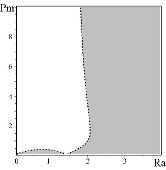
Figure 1: On the the parameter plane (Ra,Pm)𝑅𝑎𝑃𝑚(Ra,Pm) the gray area shows the γ>1𝛾1\gamma>1 and the white shows the region γ<1𝛾1\gamma<1.

Here we use the notation W~1=1W1subscript~𝑊11subscript𝑊1{\widetilde{W}_{1}}=1-{W_{1}}, W~2=1W2subscript~𝑊21subscript𝑊2{\widetilde{W}_{2}}=1-{W_{2}} in order to shorten the recording of formulas (29)-(32). Let us note, that HD nonlinear α𝛼\alpha-effect described by the system of equations (25)-(26), is possible in presence of temperature stratification, i.e., Rayleigh number of Ra0𝑅𝑎0Ra\neq 0 and the external helical forces f00subscript𝑓00{\vec{f}_{0}}\neq 0. On the contrary, a MHD nonlinear α𝛼\alpha-effect occurs, when there is no heating of Ra=0𝑅𝑎0Ra=0. In the non electroconductive medium with σ=0𝜎0\sigma=0, the equation (25)-(26) coincide with the results of [16], [17]. Like in [17], we consider first of all the stability of the small field disturbances (linear theory), and then examine the possibility of the existence of stationary structures.

4 Large-scale instability

Let us consider the initial stage of development of the perturbations (W1,W2)subscript𝑊1subscript𝑊2({W_{1}},{W_{2}}) and (H1,H2)subscript𝐻1subscript𝐻2({H_{1}},{H_{2}}). Then, for small values of W1,W2subscript𝑊1subscript𝑊2{W_{1}},{W_{2}} and H1,H2subscript𝐻1subscript𝐻2{H_{1}},{H_{2}} the equations (25)-(28) are linearized and can be reduced to the following system of linear equations:

TW1Z2W1+αZW2=0subscript𝑇subscript𝑊1superscriptsubscript𝑍2subscript𝑊1𝛼subscript𝑍subscript𝑊20{\partial_{T}}{W_{1}}-\nabla_{Z}^{2}{W_{1}}+\alpha{\nabla_{Z}}{W_{2}}=0 (33)
TW2Z2W2αZW1=0subscript𝑇subscript𝑊2superscriptsubscript𝑍2subscript𝑊2𝛼subscript𝑍subscript𝑊10{\partial_{T}}{W_{2}}-\nabla_{Z}^{2}{W_{2}}-\alpha{\nabla_{Z}}{W_{1}}=0 (34)
TH1Z2H1αHZH2=0subscript𝑇subscript𝐻1superscriptsubscript𝑍2subscript𝐻1subscript𝛼𝐻subscript𝑍subscript𝐻20{\partial_{T}}{H_{1}}-\nabla_{Z}^{2}{H_{1}}-{\alpha_{H}}{\nabla_{Z}}{H_{2}}=0 (35)
TH2Z2H2+αHZH1=0subscript𝑇subscript𝐻2superscriptsubscript𝑍2subscript𝐻2subscript𝛼𝐻subscript𝑍subscript𝐻10{\partial_{T}}{H_{2}}-\nabla_{Z}^{2}{H_{2}}+{\alpha_{H}}{\nabla_{Z}}{H_{1}}=0 (36)

where

α=Ra(42Ra)(4+Ra2)2for numbersPr=1formulae-sequence𝛼𝑅𝑎42𝑅𝑎superscript4𝑅superscript𝑎22for numbers𝑃𝑟1\alpha=-\frac{{Ra(4-2Ra)}}{{{{(4+R{a^{2}})}^{2}}}}\quad\text{for numbers}\quad Pr=1 (37)
αH=2Pm(1+Pm2)(4+Ra2)subscript𝛼𝐻2𝑃𝑚1𝑃superscript𝑚24𝑅superscript𝑎2{\alpha_{H}}=\frac{{2Pm}}{{\left({1+P{m^{2}}}\right)(4+R{a^{2}})}} (38)

From the equations (33)-(36) we can see that under small perturbations of fields the self-consistent system of equations (25)-(28) splis into two pairs of equations for large-scale field W𝑊\vec{W} and magnetic field H𝐻\vec{H} respectively. The first pair of equations (33)-(34) are similar to the hydrodynamic equations for α𝛼\alpha-effect [7], [9], wich generate large-scale vortex structures. The second pair of equations (35)-(36) describes a well-known theory of the dynamo [3] - [5], [19], the α𝛼\alpha-effect amplifies the large-scale magnetic field by the small-scale helical turbulence. In the linear theory considered here, the generation coefficients α𝛼\alpha and αHsubscript𝛼𝐻{\alpha_{H}} do not depend on fields amplitudes but depend only on the characteristics of the medium. For the study of large-scale instability, described by the equations (33)-(36), we choose perturbations of velocity (W1,W2)subscript𝑊1subscript𝑊2({W_{1}},{W_{2}}) and magnetic induction (H1,H2)subscript𝐻1subscript𝐻2({H_{1}},{H_{2}}) in the form of flat circular polarized waves:

W1=AWexp(Γt)sinKZ,W2=BWexp(Γt)cosKZformulae-sequencesubscript𝑊1subscript𝐴𝑊Γ𝑡𝑠𝑖𝑛𝐾𝑍subscript𝑊2subscript𝐵𝑊Γ𝑡𝐾𝑍{W_{1}}={A_{W}}\exp\left({\Gamma t}\right)\;sinKZ,\;{W_{2}}={B_{W}}\exp\left({\Gamma t}\right)\;\cos KZ (39)
H1=AHexp(Γt)sinKZ,H2=BHexp(Γt)cosKZformulae-sequencesubscript𝐻1subscript𝐴𝐻Γ𝑡𝑠𝑖𝑛𝐾𝑍subscript𝐻2subscript𝐵𝐻Γ𝑡𝐾𝑍{H_{1}}={A_{H}}\exp\left({\Gamma t}\right)\;sinKZ,\;{H_{2}}={B_{H}}\exp\left({\Gamma t}\right)\;\cos KZ (40)
Refer to caption
Refer to caption
Refer to caption
Refer to caption
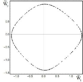
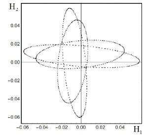
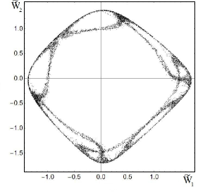
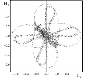
Figure 2: Poincare section for two trajectories. The upper, for the trajectory with the initial conditions W~1(0)=0.8subscript~𝑊100.8{\widetilde{W}_{1}}(0)=0.8, W~2(0)=0.8subscript~𝑊200.8{\widetilde{W}_{2}}(0)=0.8, H1(0)=0.01subscript𝐻100.01{H_{1}}(0)=0.01, H2(0)=0.01subscript𝐻200.01{H_{2}}(0)=0.01 and the lower with the initial conditions W~1(0)=0.9subscript~𝑊100.9{\widetilde{W}_{1}}(0)=0.9, W~2(0)=0.9subscript~𝑊200.9{\widetilde{W}_{2}}(0)=0.9, H1(0)=0.01subscript𝐻100.01{H_{1}}(0)=0.01, H2(0)=0.01subscript𝐻200.01{H_{2}}(0)=0.01. For the left figures, the cutting plane is stretched to single coordinate vectors of the velocity, and for the right ones to coordinate vectors of the magnetic field. One can see that the trajectory corresponding to the upper figures is wounded on tori. These trajectories are regular. The lower figures show stochastic layers. The corresponding chaotic trajectories belong to them.

Substituting (39) in the system of equations (33)-(34), and (40) in (35)-(36), we obtain two instability increments:

Γ1=±αKK2subscriptΓ1plus-or-minus𝛼𝐾superscript𝐾2{\Gamma_{1}}=\pm\alpha K-{K^{2}} (41)
Γ2=±αHKK2Pm1subscriptΓ2plus-or-minussubscript𝛼𝐻𝐾superscript𝐾2𝑃superscript𝑚1{\Gamma_{2}}=\pm{\alpha_{H}}K-{K^{2}}P{m^{-1}} (42)

The growing solution with the first increment, describes the generation of helical vortex structures of Beltrami type. The maximum of increment Γ1max=α24subscriptΓ1𝑚𝑎𝑥superscript𝛼24{\Gamma_{1max}}=\frac{{{\alpha^{2}}}}{4} is reached at Kmax=α2subscript𝐾𝑚𝑎𝑥𝛼2{K_{max}}=\frac{\alpha}{2}. In the same way, we find from formula (42) the maximum increment of large-scale magnetic field generation Γ2max=αH24PmsubscriptΓ2𝑚𝑎𝑥superscriptsubscript𝛼𝐻24𝑃𝑚{\Gamma_{2max}}=\frac{{\alpha_{H}^{2}}}{4}Pm at Kmax=αH2Pmsubscript𝐾𝑚𝑎𝑥subscript𝛼𝐻2𝑃𝑚{K_{max}}=\frac{{{\alpha_{H}}}}{2}Pm.

If the external force has zero helicity F0rotF0=0subscript𝐹0𝑟𝑜𝑡subscript𝐹00{\vec{F}_{0}}rot{\vec{F}_{0}}=0, the two α𝛼\alpha-effects disappear: α=0𝛼0\alpha=0, αH=0subscript𝛼𝐻0{\alpha_{H}}=0. In addition, when the temperature gradient is vanishing, the hydrodynamic α𝛼\alpha-effect also disappears, but MHD α𝛼\alpha-effect remains. So in these conditions, the magnetic field continues to grow. In order to understand for which Rayleigh number Ra𝑅𝑎Ra are generated large-scale vortices or magnetic disturbances it is convenient to introduce the coefficient of relative growth rate of perturbations γ=Γ1max/Γ2max𝛾subscriptΓ1subscriptΓ2\gamma={\Gamma_{1\max}}/{\Gamma_{2\max}}:

γ=Γ1maxΓ2max=Ra2(42Ra)2(1+Pm2)24Pm3(4+Ra2)2𝛾subscriptΓ1𝑚𝑎𝑥subscriptΓ2𝑚𝑎𝑥𝑅superscript𝑎2superscript42𝑅𝑎2superscript1𝑃superscript𝑚224𝑃superscript𝑚3superscript4𝑅superscript𝑎22\gamma=\frac{{{\Gamma_{1max}}}}{{{\Gamma_{2max}}}}=\frac{{R{a^{2}}{{(4-2Ra)}^{2}}{{(1+P{m^{2}})}^{2}}}}{{4P{m^{3}}{{(4+R{a^{2}})}^{2}}}} (43)

From this we can see that at small magnetic Prandtl Pm1much-less-than𝑃𝑚1Pm\ll 1 and Rayleigh numbers of Ra>2𝑅𝑎2Ra>2 there is the most effective generation of large-scale vortex disturbances. The small magnetic Prandtl numbers of Pm𝑃𝑚Pm can be due to the low electrical conductivity (σ0)𝜎0(\sigma\to 0) medium and very low kinematic viscosity (ν0)𝜈0(\nu\to 0) of medium. Now consider the case of low electroconductivity medium (σ0)𝜎0(\sigma\to 0) with ν0𝜈0\nu\neq 0, then the magnetic number of Prandtl and Chandrasekhar number are small : Pm0𝑃𝑚0Pm\to 0, Q0𝑄0Q\to 0. In this medium, the generation of large-scale magnetic field is not effective H1,21much-less-thansubscript𝐻121{H_{1,2}}\ll 1 because the coefficient γ1much-greater-than𝛾1\gamma\gg 1, and under the influence of external helical small-scale force the generation of large-scale vortex structures is possible in the convective medium which are described in detail in works [16], [17]. We turn now to the case of an electrically conductive medium, i.e., when the magnetic number of Prandtl is non zero Pm0𝑃𝑚0Pm\neq 0. From the numerical analysis of the formula (43) (see fig.1) it follows that the generation of vortex disturbances is most effecient when Rayleigh numbers are Ra>2𝑅𝑎2Ra>2. White area in the figure1 shows the area of the preferential generation of magnetic disturbances. We can state that the magnetic field generation is most effective for Rayleigh numbers in the interval Ra[0,2]𝑅𝑎02Ra\in[0,2]. The linear theory is not correct when the large-scale perturbations are strong enough. Therefore it is necessary to take into account the nonlinear effects.

5 Stationary nonlinear magnetic structures

We turn now to a discussion of the nonlinear stage. Taking into account the dependence of the right sides of the system of nonlinear equations of W𝑊\vec{W}, H𝐻\vec{H}, one would expect that with the growth of perturbations the nonlinear coefficients of α(1)superscript𝛼1{\alpha^{(1)}}, α(2)superscript𝛼2{\alpha^{(2)}}, αH(1)superscriptsubscript𝛼𝐻1\alpha_{H}^{(1)}, αH(2)superscriptsubscript𝛼𝐻2\alpha_{H}^{(2)} decrease and the instability is stabilized. As a result the nonlinear stationary structures are formed. To describe these structures let us examine the nonlinear system of equations (25) - (28) in the stationary case, taking TW1=TW2=TH1=TH2=0subscript𝑇subscript𝑊1subscript𝑇subscript𝑊2subscript𝑇subscript𝐻1subscript𝑇subscript𝐻20{\partial_{T}}{W_{1}}={\partial_{T}}{W_{2}}={\partial_{T}}{H_{1}}={\partial_{T}}{H_{2}}=0. Integrating these equations on Z𝑍Z we obtain:

dW~1dZ=α(2)W~2(1QH22Pm1+Pm2W~22)+C1𝑑subscript~𝑊1𝑑𝑍superscript𝛼2subscript~𝑊21𝑄superscriptsubscript𝐻22𝑃𝑚1𝑃superscript𝑚2superscriptsubscript~𝑊22subscript𝐶1\frac{{d{{\widetilde{W}}_{1}}}}{{dZ}}={\alpha^{(2)}}{\widetilde{W}_{2}}\left({1-\frac{{QH_{2}^{2}Pm}}{{1+P{m^{2}}\widetilde{W}_{2}^{2}}}}\right)+{C_{1}} (44)
dW~2dZ=α(1)W~1(1QH12Pm1+Pm2W~12)+C2𝑑subscript~𝑊2𝑑𝑍superscript𝛼1subscript~𝑊11𝑄superscriptsubscript𝐻12𝑃𝑚1𝑃superscript𝑚2superscriptsubscript~𝑊12subscript𝐶2\frac{{d{{\widetilde{W}}_{2}}}}{{dZ}}=-{\alpha^{(1)}}{\widetilde{W}_{1}}\left({1-\frac{{QH_{1}^{2}Pm}}{{1+P{m^{2}}\widetilde{W}_{1}^{2}}}}\right)+{C_{2}} (45)
1PmdH1dZ=αH(2)H2+C31𝑃𝑚𝑑subscript𝐻1𝑑𝑍superscriptsubscript𝛼𝐻2subscript𝐻2subscript𝐶3\frac{1}{{Pm}}\frac{{d{H_{1}}}}{{dZ}}=-\alpha_{H}^{(2)}{H_{2}}+{C_{3}} (46)
1PmdH2dZ=αH(1)H1+C41𝑃𝑚𝑑subscript𝐻2𝑑𝑍superscriptsubscript𝛼𝐻1subscript𝐻1subscript𝐶4\frac{1}{{Pm}}\frac{{d{H_{2}}}}{{dZ}}=\alpha_{H}^{(1)}{H_{1}}+{C_{4}} (47)

Here C1subscript𝐶1{C_{1}}, C2subscript𝐶2{C_{2}}, C3subscript𝐶3{C_{3}}, C4subscript𝐶4{C_{4}} are arbitrary constants of integration. Equations (44) - (47) present the nonlinear dynamical system in four-dimensional phase space. It can be proved that this system of equations is conservative. However to find the Hamiltonian of this nonlinear system is technically bulky task. Even if it exists, it can only be obtained in quadratures and the execution of integration removes it beyond the class of elementary functions.

Refer to caption
Refer to caption
Refer to caption
Refer to caption
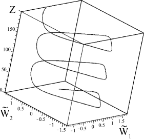
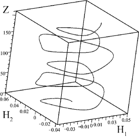
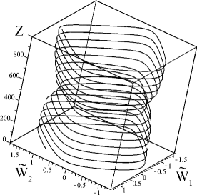
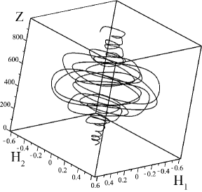
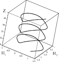
Figure 3: The upper part shows the velocity and magnetic field dependence on the height for the numerical solution of equations (44) - (47) with the initial conditions: W~1(0)=0.8subscript~𝑊100.8{\widetilde{W}_{1}}(0)=0.8, W~2(0)=0.8subscript~𝑊200.8{\widetilde{W}_{2}}(0)=0.8, H1(0)=0.01subscript𝐻100.01{H_{1}}(0)=0.01, H2(0)=0.01subscript𝐻200.01{H_{2}}(0)=0.01. This dependence corresponds to regular motion of the Poincare section shown on top of Fig. 2. Below a similar dependence for the numerical solution of equations ((44)) - ((47)) with the initial conditions: W~1(0)=0.9subscript~𝑊100.9{\widetilde{W}_{1}}(0)=0.9, W~2(0)=0.9subscript~𝑊200.9{\widetilde{W}_{2}}(0)=0.9, H1(0)=0.01subscript𝐻100.01{H_{1}}(0)=0.01, H2(0)=0.01subscript𝐻200.01{H_{2}}(0)=0.01. This chaotic dependence corresponds to Poincare sections in Fig.2 shown at the bottom.

In general case this conservative nonlinear system of four coupled equations has no attractors in phase space. The high dimensionality of the phase space and a large number of parameters in the system make very diffucult the full qualitative analysis of this system. One of the common features is the invariance of the system under the transformation (W~1,W~2,H1,H2)(W~1,W~2,H1,H2)subscript~𝑊1subscript~𝑊2subscript𝐻1subscript𝐻2subscript~𝑊1subscript~𝑊2subscript𝐻1subscript𝐻2({\widetilde{W}_{1}},{\widetilde{W}_{2}},{H_{1}},{H_{2}})\to(-{\widetilde{W}_{1}},-{\widetilde{W}_{2}},-{H_{1}},-{H_{2}}). With zero constant C1=C2=C3=C4=0subscript𝐶1subscript𝐶2subscript𝐶3subscript𝐶40{C_{1}}={C_{2}}={C_{3}}={C_{4}}=0 in the phase space a fixed point exists at the origin of the phase space. In the phase space of such a system the presence of resonant and nonresonant tori can be expected. In its turn this means the existence of chaotic stationary structures of hydrodynamic and magnetic fields. To prove the existence of these stationary trajectories let us consider the Poincare section of the trajectories in the phase space. Fig.2 shows examples of the cross-sections obtained numerically for the dimensionless parameters Q=Pm=Pr=1𝑄𝑃𝑚𝑃𝑟1Q=Pm=Pr=1, Ra=2𝑅𝑎2Ra=2 and the constants C1=C2=0.01subscript𝐶1subscript𝐶20.01{C_{1}}={C_{2}}=0.01, C3=C4=0.001subscript𝐶3subscript𝐶40.001{C_{3}}={C_{4}}=0.001. The upper part of Fig.2 demonstrates the Poincare section of regular trajectory for the velocity and magnetic fields. The structure of the chaotic layer, which belongs to the selected path is clearly visible on the lower section. The presence of such chaotic trajectories implies the existence of a stationary random structure of the velocity and magnetic fields. The chaotic change of velocity direction of magnetic fields according to the height Z𝑍Z is typical for these trajectories. Thus this set of equations has stationary chaotic solutions. Fig.3 shows the dependence of stationary large-scale fields on the height of Z𝑍Z, which was obtained numerically for the initial conditions, which correspond to the Poincare sections in Fig.2. These figures show also the appearance of stationary random solutions for magnetic and vortex fields. It should be noted that the structure of the magnetic field at the bottom of Fig.3 demonstrates with the increasing of height the intermittency structure. In the numerical solution of equations (44)-(47) occur chaotic structures observed with the increase of the initial velocity amplitudes. For small initial velocities and magnetic fields regular trajectories are typical. With increasing of velocity amplitude, above a certain critical value the chaotic trajectories appear. With increasing of the initial velocity the part of the space occupied by the chaotic trajectories points grows on the Poincare sections. Under these conditions, typical solutions become chaotic.

Let us now consider in more detail which nonlinear structure may occur in the convective electrically conductive turbulent medium, in some limit cases. Let us suppose that the generation of large-scale vortex disturbances in the convective medium is not yet in the stationary mode, but large-scale perturbations of the magnetic field are already reached their saturation on stationary level. Then the influence of the small amplitude of large-scale vortex disturbances W1,21much-less-thansubscript𝑊121{W_{1,2}}\ll 1 on the evolution of large-scale magnetic fields can be neglected. As a result, from the equations of the nonlinear dynamo (25) - (28), we obtain the equations for the evolution of the large-scale stationary magnetic field:

dH1dZ=H2(Q2H24+RaQH22+4)(Q2H24+4)(Q2H24+2RaQH22+Ra2+4)+C3𝑑subscript𝐻1𝑑𝑍subscript𝐻2superscript𝑄2superscriptsubscript𝐻24𝑅𝑎𝑄superscriptsubscript𝐻224superscript𝑄2superscriptsubscript𝐻244superscript𝑄2superscriptsubscript𝐻242𝑅𝑎𝑄superscriptsubscript𝐻22𝑅superscript𝑎24subscript𝐶3\frac{{d{H_{1}}}}{{dZ}}=-\frac{{{H_{2}}({Q^{2}}H_{2}^{4}+RaQH_{2}^{2}+4)}}{{({Q^{2}}H_{2}^{4}+4)({Q^{2}}H_{2}^{4}+2RaQH_{2}^{2}+R{a^{2}}+4)}}+{C_{3}} (48)
dH2dZ=H1(Q2H14+RaQH12+4)(Q2H14+4)(Q2H14+2RaQH12+Ra2+4)+C4𝑑subscript𝐻2𝑑𝑍subscript𝐻1superscript𝑄2superscriptsubscript𝐻14𝑅𝑎𝑄superscriptsubscript𝐻124superscript𝑄2superscriptsubscript𝐻144superscript𝑄2superscriptsubscript𝐻142𝑅𝑎𝑄superscriptsubscript𝐻12𝑅superscript𝑎24subscript𝐶4\frac{{d{H_{2}}}}{{dZ}}=\frac{{{H_{1}}({Q^{2}}H_{1}^{4}+RaQH_{1}^{2}+4)}}{{({Q^{2}}H_{1}^{4}+4)({Q^{2}}H_{1}^{4}+2RaQH_{1}^{2}+R{a^{2}}+4)}}+{C_{4}} (49)

Here, to simplify the calculation we use the Prandtl numbers: Pr=Pm=1𝑃𝑟𝑃𝑚1Pr=Pm=1.

Refer to caption
Refer to caption
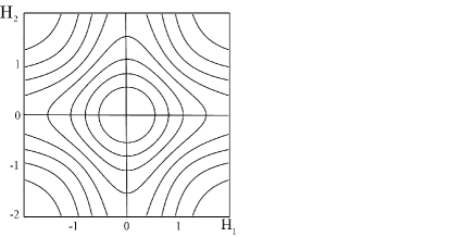
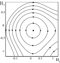
Figure 4: On the left the phase portrait of Hamiltonian equations (51) at C3=C4=0subscript𝐶3subscript𝐶40{C_{3}}={C_{4}}=0; on the right, the solution corresponding to the nonlinear wave.

Equation (48)-(49) can be written in the Hamiltonian form:

dX~dt=ddP~,dP~dt=ddX~formulae-sequence𝑑~𝑋𝑑𝑡𝑑𝑑~𝑃𝑑~𝑃𝑑𝑡𝑑𝑑~𝑋\frac{{d\widetilde{X}}}{{dt}}=-\frac{{d{\cal H}}}{{d\widetilde{P}}},\;\;\frac{{d\widetilde{P}}}{{dt}}=\frac{{d{\cal H}}}{{d\widetilde{X}}} (50)

where we have introduced new variables X~=QH1~𝑋𝑄subscript𝐻1\widetilde{X}=\sqrt{Q}{H_{1}}, P~=QH2~𝑃𝑄subscript𝐻2\widetilde{P}=\sqrt{Q}{H_{2}}, t=Z𝑡𝑍t=Z. The Hamiltonian of the magnetic field {\cal H} is of the form:

=U(P~)+U(X~)C~3P+C~4X+C5𝑈~𝑃𝑈~𝑋subscript~𝐶3𝑃subscript~𝐶4𝑋subscript𝐶5{\cal H}=U(\widetilde{P})+U(\widetilde{X})-{\widetilde{C}_{3}}P+{\widetilde{C}_{4}}X+{C_{5}} (51)

where the function U(y)𝑈𝑦U(y) is equal to:

U(y)=Ra4(Ra2+16)ln(y4+4y4+4+2Ray2+Ra2)+𝑈𝑦limit-from𝑅𝑎4𝑅superscript𝑎216superscript𝑦44superscript𝑦442𝑅𝑎superscript𝑦2𝑅superscript𝑎2U(y)=\frac{{Ra}}{{4(R{a^{2}}+16)}}\ln\left({\frac{{{y^{4}}+4}}{{{y^{4}}+4+2Ra{y^{2}}+R{a^{2}}}}}\right)+
+2Ra2+16(arctg(y22)+arctg(y2+Ra2))2𝑅superscript𝑎216𝑎𝑟𝑐𝑡𝑔superscript𝑦22𝑎𝑟𝑐𝑡𝑔superscript𝑦2𝑅𝑎2+\frac{2}{{R{a^{2}}+16}}\left({arctg\left({\frac{{{y^{2}}}}{2}}\right)+arctg\left({\frac{{{y^{2}}+Ra}}{2}}\right)}\right) (52)

The constant C~3subscript~𝐶3{\widetilde{C}_{3}} and C~4subscript~𝐶4{\widetilde{C}_{4}}, respectively, are: C~3=QC3subscript~𝐶3𝑄subscript𝐶3{\widetilde{C}_{3}}=\sqrt{Q}{C_{3}}, C~4=QC4subscript~𝐶4𝑄subscript𝐶4{\widetilde{C}_{4}}=\sqrt{Q}{C_{4}}. We examine now the the types of stationary magnetic structures described by equations (50). First of all we consider in detail the limit case Ra0𝑅𝑎0Ra\to 0. Then the Hamiltonian (51) takes the following form:

=14Qarctg(QH122)+14Qarctg(QH222)+C4H1C3H2+C~5superscript14𝑄𝑎𝑟𝑐𝑡𝑔𝑄superscriptsubscript𝐻12214𝑄𝑎𝑟𝑐𝑡𝑔𝑄superscriptsubscript𝐻222subscript𝐶4subscript𝐻1subscript𝐶3subscript𝐻2subscript~𝐶5{\cal H}\to{\cal H}^{\prime}=\frac{1}{{4Q}}arctg\left({\frac{{QH_{1}^{2}}}{2}}\right)+\frac{1}{{4Q}}arctg\left({\frac{{QH_{2}^{2}}}{2}}\right)+{C_{4}}{H_{1}}-{C_{3}}{H_{2}}+{\widetilde{C}_{5}} (53)

The Hamiltonian equations (50) mean that in the phase space only fixed points of two types can be observed: elliptical and hyperbolic fixed points. At zero values of the constants C3=C4=0subscript𝐶3subscript𝐶40{C_{3}}={C_{4}}=0 it is possible to construct the phase portrait of Hamiltonian (53) from which it is clear that there is only one elliptic point (see Fig.4). Around the elliptic points are observed the nonlinear waves only. The numerical stationary solution of equations (48)-(49) in the limit of Ra0𝑅𝑎0Ra\to 0 corresponds to a nonlinear wave of finite amplitude and is shown in Fig.4. Calculating the maximum and minimum of (H1,2Q2H1,24+4)subscript𝐻12superscript𝑄2superscriptsubscript𝐻1244\left({\frac{{{H_{1,2}}}}{{{Q^{2}}H_{1,2}^{4}+4}}}\right) we find the area of the parameter (C3,C4)subscript𝐶3subscript𝐶4({C_{3}},{C_{4}}) change defined by the inequalities:

χ<C3<χ𝜒subscript𝐶3𝜒-\chi<{C_{3}}<\chi
χ<C4<χ𝜒subscript𝐶4𝜒-\chi<{C_{4}}<\chi

where χ=33/4162Q𝜒superscript334162𝑄\chi=\frac{{{3^{3/4}}}}{{16}}\sqrt{\frac{2}{Q}} depends on the choice of the parameter Q𝑄Q.

Refer to caption
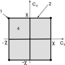
Figure 5: On the parameter plane (C3,C4)subscript𝐶3subscript𝐶4({C_{3}},{C_{4}}) gray area shows the presence of four fixed points. For constants (C3=0,C4=0)formulae-sequencesubscript𝐶30subscript𝐶40({C_{3}}=0,{C_{4}}=0), there is only one fixed point. The bold lines mark the values of the constants which correspond to the two fixed points on phase portrait. The vertices of the square area correspond to the values at which exist one fixed point. For values outside this area fixed points are absent.

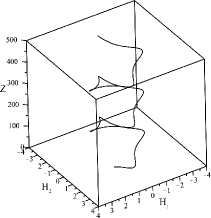
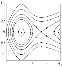
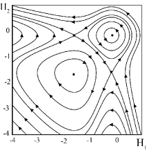
In Fig.5 the corresponding area is presented with the number of fixed points. In the vertices of square area of the parameters (C3,C4)subscript𝐶3subscript𝐶4({C_{3}},{C_{4}}) is located a fixed point of the elliptical type. The type of fixed point is determined by the form of phase portrait of Hamiltonian (53) for the constants C3=±χsubscript𝐶3plus-or-minus𝜒{C_{3}}=\pm\chi and C4=±χsubscript𝐶4plus-or-minus𝜒{C_{4}}=\pm\chi (see Fig.6). On the boundary of (C3,C4)subscript𝐶3subscript𝐶4({C_{3}},{C_{4}}) are two fixed points: the elliptical and hyperbolic one. Phase portrait for these points is shown in Fig.6. For constants (C3=0,C4=([χ,0[,]0,χ]))({C_{3}}=0,{C_{4}}=([-\chi,0[,]0,-\chi])), C3=([χ,0[,]0,χ]),C4=0){C_{3}}=([-\chi,0[,]0,-\chi]),{C_{4}}=0) there are also two fixed points: the elliptical and hyperbolic one. The phase portrait for this point is shown in Fig.6. At last, within each sector of the area (C3,C4)subscript𝐶3subscript𝐶4({C_{3}},{C_{4}}) are four fixed points, two elliptical and two hyperbolic. Phase portraits for these points, are shown in Fig.6. Fig.7 shows a three-dimensional image of the limited stationary structures corresponding to the phase portraits presented in Fig.7. The left side of Fig.7 shows the numerical solution corresponding to a nonlinear wave that occurs in the vicinity of elliptic point in the phase space. The central part of Fig.7 shows the solitons solution, which correspond to the separatrix part going out and in the hyperbolic point. Finally, the right side of Fig.7 presents a solution for the kink, which corresponds to the part of the separatrix linking two hyperbolic points.

Refer to caption
Refer to caption
Refer to caption
Figure 6: On the left the phase portrait for the fixed points located at vertices of the square area of parameters (C3,C4)subscript𝐶3subscript𝐶4({C_{3}},{C_{4}}); the center-phase portrait for the fixed points on the boundary of the parameters (C3,C4)subscript𝐶3subscript𝐶4({C_{3}},{C_{4}}), fixed points when (C3=0,C4=±χ)formulae-sequencesubscript𝐶30subscript𝐶4plus-or-minus𝜒({C_{3}}=0,{C_{4}}=\pm\chi); (C3=±χ,C4=0)formulae-sequencesubscript𝐶3plus-or-minus𝜒subscript𝐶40({C_{3}}=\pm\chi,{C_{4}}=0); on the right the phase portrait for the fixed points inside the square area of parameters (C3,C4)subscript𝐶3subscript𝐶4({C_{3}},{C_{4}}).

Let us now turn to the evolution of large-scale stationary magnetic field for the case when the Rayleigh number Ra2𝑅𝑎2Ra\to 2. In this limit, the Hamiltonian (51) takes the following form:

=140Qln(Q2H14+4Q2H14+4QH12+8)+140Qln(Q2H24+4Q2H24+4QH22+8)+superscript140𝑄superscript𝑄2superscriptsubscript𝐻144superscript𝑄2superscriptsubscript𝐻144𝑄superscriptsubscript𝐻128limit-from140𝑄superscript𝑄2superscriptsubscript𝐻244superscript𝑄2superscriptsubscript𝐻244𝑄superscriptsubscript𝐻228{\cal H}\to{\cal H}^{\prime}=\frac{1}{{40Q}}\ln\left({\frac{{{Q^{2}}H_{1}^{4}+4}}{{{Q^{2}}H_{1}^{4}+4QH_{1}^{2}+8}}}\right)+\frac{1}{{40Q}}\ln\left({\frac{{{Q^{2}}H_{2}^{4}+4}}{{{Q^{2}}H_{2}^{4}+4QH_{2}^{2}+8}}}\right)+
+110Qarctg(4(QH12+1)4Q2H142QH12)+110Qarctg(4(QH22+1)4Q2H242QH22)110𝑄𝑎𝑟𝑐𝑡𝑔4𝑄superscriptsubscript𝐻1214superscript𝑄2superscriptsubscript𝐻142𝑄superscriptsubscript𝐻12110𝑄𝑎𝑟𝑐𝑡𝑔4𝑄superscriptsubscript𝐻2214superscript𝑄2superscriptsubscript𝐻242𝑄superscriptsubscript𝐻22+\frac{1}{{10Q}}arctg\left({\frac{{4(QH_{1}^{2}+1)}}{{4-{Q^{2}}H_{1}^{4}-2QH_{1}^{2}}}}\right)+\frac{1}{{10Q}}arctg\left({\frac{{4(QH_{2}^{2}+1)}}{{4-{Q^{2}}H_{2}^{4}-2QH_{2}^{2}}}}\right)
+C4H1C3H2+C~5subscript𝐶4subscript𝐻1subscript𝐶3subscript𝐻2subscript~𝐶5+{C_{4}}{H_{1}}-{C_{3}}{H_{2}}+{\widetilde{C}_{5}} (54)

At zero values of the constants C3=C4=0subscript𝐶3subscript𝐶40{C_{3}}={C_{4}}=0 the phase portrait of Hamiltonian ((54)) is similar to the Fig.4. which implies the appearance of only one elliptic point in the phase space. In this case, all appearing stationary solutions coincide with the nonlinear waves. The stationary solution corresponding to the nonlinear finite amplitude wave are similar to the Fig.4.

As in the previous case it is easy to set the parameters for the area C3,C4subscript𝐶3subscript𝐶4{C_{3}},{C_{4}} with a different number of fixed points. We notice that the region of existence of fixed points of the parameter plane (C3,C4)subscript𝐶3subscript𝐶4({C_{3}},{C_{4}}) is determined by the inequalities:

χ~<C3<χ~~𝜒subscript𝐶3~𝜒-\widetilde{\chi}<{C_{3}}<\widetilde{\chi}
χ~<C4<χ~~𝜒subscript𝐶4~𝜒-\widetilde{\chi}<{C_{4}}<\widetilde{\chi}

where χ~=max(H1(Q2H14+RaQH12+4)(Q2H14+4)(Q2H14+2RaQH12+Ra2+4))~𝜒subscript𝐻1superscript𝑄2superscriptsubscript𝐻14𝑅𝑎𝑄superscriptsubscript𝐻124superscript𝑄2superscriptsubscript𝐻144superscript𝑄2superscriptsubscript𝐻142𝑅𝑎𝑄superscriptsubscript𝐻12𝑅superscript𝑎24\widetilde{\chi}=\max\left({\frac{{{H_{1}}({Q^{2}}H_{1}^{4}+RaQH_{1}^{2}+4)}}{{({Q^{2}}H_{1}^{4}+4)({Q^{2}}H_{1}^{4}+2RaQH_{1}^{2}+R{a^{2}}+4)}}}\right) when H1subscript𝐻1{H_{1}}is changing. For fixed values of the parameters Ra,Q𝑅𝑎𝑄Ra,Q, this maximum can be easily calculated. From the results of these calculations, we obtain the similar phase portraits of the Hamiltonian (54) and numerical solutions of equations (48)-(49) at Ra2𝑅𝑎2Ra\to 2 like in the previous case. Thus, comparing the growth rate of the vortex and magnetic disturbances at the initial stage of large-scale development of the instability, we considered the emergence of large-scale stationary magnetic structures. These structures are classified as stationary solutions of three types: nonlinear waves, solitons and kinks.

6 Conclusions

In this paper the closed system of nonlinear equations was obtained using the asymptotic method. These equations describe both linear and nonlinear increase stages of hydrodynamic flows and magnetic fields in a electroconducting medium. This system of equations allows to explain emergence and stabilization of large-scale magnetic fields of some astrophysical objects, stars, in particular. It is also interesting to use it to describe the generation of large-scale fields by convection in electrically conductive medium in the interior of planets. It should be noted that despite the asymptotic technique based on the presence of small-scale oscillations that is used, it is expected that the results can be applicable to the turbulent media. The turbulent case has the whole range of these small-scale oscillations. Qualitative evaluation of the linear stage for the solar conditions [20] allow us to state a good coincidence of the resulting hydrodynamic structures characteristic scales and times with observation data [21]. This fact suggests that other stationary magneto-hydrodynamic structures, like soliton exist in the Sun photosphere.

Refer to caption
Refer to caption
Refer to caption
Figure 7: The numerical stationary solutions of equations (48) - (49) at Ra0𝑅𝑎0Ra\to 0 in the form of nonlinear wave, soliton and kink. They correspond to the phase portraits, shown in Figure 4.

Appendix I. Multiscale asymptotic developments

Let us find the algebraic structure of the asymptotic development in various orders of R𝑅R, starting with the lowest. In order of R3superscript𝑅3{R^{-3}} there is only one equation:

iP3=0P3=P3(X)subscript𝑖subscript𝑃30subscript𝑃3subscript𝑃3𝑋{\partial_{i}}{P_{-3}}=0\Rightarrow\;{P_{-3}}={P_{-3}}(X) (55)

In order R2superscript𝑅2{R^{-2}} appears equation:

iP2=0P2=P2(X){\partial_{i}}{P_{-2}}=0\quad\quad\Rightarrow\;\;{P_{-2}}={P_{-2}}\left(X\right) (56)

Consequently, quantities P3subscript𝑃3{P_{-3}} and P2subscript𝑃2{P_{-2}} depend only on fast variables. In order R1superscript𝑅1{R^{-1}}, we obtain more complicated system of equations:

tW1i+W1kkW1i=iP1iP3+k2W1i+subscript𝑡superscriptsubscript𝑊1𝑖superscriptsubscript𝑊1𝑘subscript𝑘superscriptsubscript𝑊1𝑖subscript𝑖subscript𝑃1subscript𝑖subscript𝑃3limit-fromsuperscriptsubscript𝑘2superscriptsubscript𝑊1𝑖{\partial_{t}}W_{-1}^{i}+W_{-1}^{k}{\partial_{k}}W_{-1}^{i}=-{\partial_{i}}{P_{-1}}-{\nabla_{i}}{P_{-3}}+\partial_{k}^{2}W_{-1}^{i}+
+Ra~eiT1+Q~εijkεjmlmB1lB1k~𝑅𝑎subscript𝑒𝑖subscript𝑇1~𝑄subscript𝜀𝑖𝑗𝑘subscript𝜀𝑗𝑚𝑙subscript𝑚superscriptsubscript𝐵1𝑙superscriptsubscript𝐵1𝑘+\widetilde{Ra}{e_{i}}{T_{-1}}+\widetilde{Q}{\varepsilon_{ijk}}{\varepsilon_{jml}}{\partial_{m}}B_{-1}^{l}B_{-1}^{k} (57)
tB1iPm1k2B1i=εijkεknpjW1nB1psubscript𝑡superscriptsubscript𝐵1𝑖𝑃superscript𝑚1superscriptsubscript𝑘2superscriptsubscript𝐵1𝑖subscript𝜀𝑖𝑗𝑘subscript𝜀𝑘𝑛𝑝subscript𝑗superscriptsubscript𝑊1𝑛superscriptsubscript𝐵1𝑝{\partial_{t}}B_{-1}^{i}-P{m^{-1}}\partial_{k}^{2}B_{-1}^{i}={\varepsilon_{ijk}}{\varepsilon_{knp}}{\partial_{j}}W_{-1}^{n}B_{-1}^{p} (58)
tT1Pr1k2T1=W1kkT1W1zsubscript𝑡subscript𝑇1𝑃superscript𝑟1superscriptsubscript𝑘2subscript𝑇1superscriptsubscript𝑊1𝑘subscript𝑘subscript𝑇1superscriptsubscript𝑊1𝑧{\partial_{t}}{T_{-1}}-P{r^{-1}}\partial_{k}^{2}{T_{-1}}=-W_{-1}^{k}{\partial_{k}}{T_{-1}}-W_{-1}^{z} (59)
iW1i=0,iB1i=0formulae-sequencesubscript𝑖superscriptsubscript𝑊1𝑖0subscript𝑖superscriptsubscript𝐵1𝑖0{\partial_{i}}W_{-1}^{i}=0,\quad\quad{\partial_{i}}B_{-1}^{i}=0 (60)

The averaging of equations (57)-(60) on the fast variables give the following secular equations:

iP3+Ra~eiT1=0subscript𝑖subscript𝑃3~𝑅𝑎subscript𝑒𝑖subscript𝑇10-{\nabla_{i}}{P_{-3}}+\widetilde{Ra}{e_{i}}{T_{-1}}=0 (61)
W1z=0superscriptsubscript𝑊1𝑧0W_{-1}^{z}=0 (62)

In zero order in R𝑅R we have the equations:

tv0i+W1kkv0i+v0kkW1i=iP0iP2+subscript𝑡superscriptsubscript𝑣0𝑖superscriptsubscript𝑊1𝑘subscript𝑘superscriptsubscript𝑣0𝑖superscriptsubscript𝑣0𝑘subscript𝑘superscriptsubscript𝑊1𝑖subscript𝑖subscript𝑃0limit-fromsubscript𝑖subscript𝑃2{\partial_{t}}v_{0}^{i}+W_{-1}^{k}{\partial_{k}}v_{0}^{i}+v_{0}^{k}{\partial_{k}}W_{-1}^{i}=-{\partial_{i}}{P_{0}}-{\nabla_{i}}{P_{-2}}+
+k2v0i+Ra~eiT0+Q~εijkεjml(mB1lB0k+mB0lB1k)+F0isuperscriptsubscript𝑘2superscriptsubscript𝑣0𝑖~𝑅𝑎subscript𝑒𝑖subscript𝑇0~𝑄subscript𝜀𝑖𝑗𝑘subscript𝜀𝑗𝑚𝑙subscript𝑚superscriptsubscript𝐵1𝑙superscriptsubscript𝐵0𝑘subscript𝑚superscriptsubscript𝐵0𝑙superscriptsubscript𝐵1𝑘superscriptsubscript𝐹0𝑖+\partial_{k}^{2}v_{0}^{i}+\widetilde{Ra}{e_{i}}{T_{0}}+\widetilde{Q}{\varepsilon_{ijk}}{\varepsilon_{jml}}\left({{\partial_{m}}B_{-1}^{l}B_{0}^{k}+{\partial_{m}}B_{0}^{l}B_{-1}^{k}}\right)+F_{0}^{i} (63)
tB0iPm1k2B0i=εijkεknp(jW1nB0p+jv0nB1p)subscript𝑡superscriptsubscript𝐵0𝑖𝑃superscript𝑚1superscriptsubscript𝑘2superscriptsubscript𝐵0𝑖subscript𝜀𝑖𝑗𝑘subscript𝜀𝑘𝑛𝑝subscript𝑗superscriptsubscript𝑊1𝑛superscriptsubscript𝐵0𝑝subscript𝑗superscriptsubscript𝑣0𝑛superscriptsubscript𝐵1𝑝{\partial_{t}}B_{0}^{i}-P{m^{-1}}\partial_{k}^{2}B_{0}^{i}={\varepsilon_{ijk}}{\varepsilon_{knp}}\left({{\partial_{j}}W_{-1}^{n}B_{0}^{p}+{\partial_{j}}v_{0}^{n}B_{-1}^{p}}\right) (64)
tT0Pr1k2T0=W1kkT0k(v0kT1)v0zsubscript𝑡subscript𝑇0𝑃superscript𝑟1superscriptsubscript𝑘2subscript𝑇0superscriptsubscript𝑊1𝑘subscript𝑘subscript𝑇0subscript𝑘superscriptsubscript𝑣0𝑘subscript𝑇1superscriptsubscript𝑣0𝑧{\partial_{t}}{T_{0}}-P{r^{-1}}\partial_{k}^{2}{T_{0}}=-W_{-1}^{k}{\partial_{k}}{T_{0}}-{\partial_{k}}(v_{0}^{k}{T_{-1}})-v_{0}^{z} (65)
iv0i=0,iB0i=0formulae-sequencesubscript𝑖superscriptsubscript𝑣0𝑖0subscript𝑖superscriptsubscript𝐵0𝑖0{\partial_{i}}v_{0}^{i}=0,\quad\quad{\partial_{i}}B_{0}^{i}=0 (66)

These equations give one secular equation:

P2=0P2=constformulae-sequencesubscript𝑃20subscript𝑃2𝑐𝑜𝑛𝑠𝑡\nabla{P_{-2}}=0\quad\quad\Rightarrow\quad\quad{P_{-2}}=const (67)

Let us consider the equations of the first approximation R1superscript𝑅1{R^{1}}:

tv1i+W1kkv1i+v0kkv0i+v1kkW1i+W1kkW1i=subscript𝑡superscriptsubscript𝑣1𝑖superscriptsubscript𝑊1𝑘subscript𝑘superscriptsubscript𝑣1𝑖superscriptsubscript𝑣0𝑘subscript𝑘superscriptsubscript𝑣0𝑖superscriptsubscript𝑣1𝑘subscript𝑘superscriptsubscript𝑊1𝑖superscriptsubscript𝑊1𝑘subscript𝑘superscriptsubscript𝑊1𝑖absent{\partial_{t}}v_{1}^{i}+W_{-1}^{k}{\partial_{k}}v_{1}^{i}+v_{0}^{k}{\partial_{k}}v_{0}^{i}+v_{1}^{k}{\partial_{k}}W_{-{1}}^{i}+W_{-{1}}^{k}{\nabla_{k}}W_{-{1}}^{i}=
=iP1i(P1+P¯1)+k2v1i+2kkW1i+Ra~eiT1+absentsubscript𝑖subscript𝑃1subscript𝑖subscript𝑃1subscript¯𝑃1superscriptsubscript𝑘2superscriptsubscript𝑣1𝑖2subscript𝑘subscript𝑘superscriptsubscript𝑊1𝑖limit-from~𝑅𝑎subscript𝑒𝑖subscript𝑇1=-{\nabla_{i}}{P_{-{1}}}-{\partial_{i}}\left({{P_{1}}+{{\overline{P}}_{1}}}\right)+\partial_{k}^{2}{v_{1}}^{i}+2{\partial_{k}}{\nabla_{k}}W_{-1}^{i}+\widetilde{Ra}{e_{i}}T_{1}+
+Q~εijkεjmlmB1lB1k+mB0lB0k+mB1lB1k+mB1lB1k)+\widetilde{Q}{\varepsilon_{ijk}}{\varepsilon_{jml}}{\partial_{m}}B_{-{1}}^{l}B_{1}^{k}+{\partial_{m}}B_{0}^{l}B_{0}^{k}+{\partial_{m}}B_{1}^{l}B_{-{1}}^{k}+{\nabla_{m}}B_{-{1}}^{l}B_{-{1}}^{k}{)} (68)
tB1iPm1k2B1iPm12kkB1i=subscript𝑡superscriptsubscript𝐵1𝑖𝑃superscript𝑚1superscriptsubscript𝑘2superscriptsubscript𝐵1𝑖𝑃superscript𝑚12subscript𝑘subscript𝑘superscriptsubscript𝐵1𝑖absent{\partial_{t}}B_{1}^{i}-P{m^{-1}}\partial_{k}^{2}B_{1}^{i}-P{m^{-1}}2{\partial_{k}}{\nabla_{k}}B_{-1}^{i}=
=εijkεknp(jW1nB1p+jv0nB0p+jv1nB1p+jW1nB1p)absentsubscript𝜀𝑖𝑗𝑘subscript𝜀𝑘𝑛𝑝subscript𝑗superscriptsubscript𝑊1𝑛superscriptsubscript𝐵1𝑝subscript𝑗superscriptsubscript𝑣0𝑛superscriptsubscript𝐵0𝑝subscript𝑗superscriptsubscript𝑣1𝑛superscriptsubscript𝐵1𝑝subscript𝑗superscriptsubscript𝑊1𝑛superscriptsubscript𝐵1𝑝={\varepsilon_{ijk}}{\varepsilon_{knp}}({\partial_{j}}W_{-1}^{n}B_{1}^{p}+{\partial_{j}}v_{0}^{n}B_{0}^{p}+{\partial_{j}}v_{1}^{n}B_{-1}^{p}+{\nabla_{j}}W_{-1}^{n}B_{-1}^{p}) (69)
tT1Pr1k2T1Pr12kkT1=subscript𝑡subscript𝑇1𝑃superscript𝑟1superscriptsubscript𝑘2subscript𝑇1𝑃superscript𝑟12subscript𝑘subscript𝑘subscript𝑇1absent{\partial_{t}}{T_{1}}-P{r^{-1}}\partial_{k}^{2}{T_{1}}-P{r^{-1}}2{\partial_{k}}{\nabla_{k}}{T_{-1}}=
=W1kkT1W1kkT1v0kkT0v1kkT1v1zabsentsuperscriptsubscript𝑊1𝑘subscript𝑘subscript𝑇1superscriptsubscript𝑊1𝑘subscript𝑘subscript𝑇1superscriptsubscript𝑣0𝑘subscript𝑘subscript𝑇0superscriptsubscript𝑣1𝑘subscript𝑘subscript𝑇1superscriptsubscript𝑣1𝑧=-W_{-1}^{k}{\partial_{k}}{T_{1}}-W_{-1}^{k}{\nabla_{k}}{T_{-1}}-v_{0}^{k}{\partial_{k}}{T_{0}}-v_{1}^{k}{\partial_{k}}{T_{-1}}-v_{1}^{z} (70)
iv1i+iW1i=0,iB1i+iB1i=0formulae-sequencesubscript𝑖superscriptsubscript𝑣1𝑖subscript𝑖superscriptsubscript𝑊1𝑖0subscript𝑖superscriptsubscript𝐵1𝑖subscript𝑖superscriptsubscript𝐵1𝑖0{\partial_{i}}v_{1}^{i}+{\nabla_{i}}W_{-1}^{i}=0,\quad\quad{\partial_{i}}B_{1}^{i}+{\nabla_{i}}B_{-1}^{i}=0 (71)

The secular equations follow from this system of equations:

W1kkW1i=iP1+Q~εijkεjmlmB1lB1ksuperscriptsubscript𝑊1𝑘subscript𝑘superscriptsubscript𝑊1𝑖subscript𝑖subscript𝑃1~𝑄subscript𝜀𝑖𝑗𝑘subscript𝜀𝑗𝑚𝑙subscript𝑚superscriptsubscript𝐵1𝑙superscriptsubscript𝐵1𝑘W_{-1}^{k}{\nabla_{k}}W_{-1}^{i}=-{\nabla_{i}}{P_{-1}}+\widetilde{Q}{\varepsilon_{ijk}}{\varepsilon_{jml}}{\nabla_{m}}B_{-1}^{l}B_{-1}^{k} (72)
εijkεknpjW1nB1p=0subscript𝜀𝑖𝑗𝑘subscript𝜀𝑘𝑛𝑝subscript𝑗superscriptsubscript𝑊1𝑛superscriptsubscript𝐵1𝑝0{\varepsilon_{ijk}}{\varepsilon_{knp}}{\nabla_{j}}W_{-1}^{n}B_{-1}^{p}=0 (73)
W1kkT1=0,superscriptsubscript𝑊1𝑘subscript𝑘subscript𝑇10W_{-1}^{k}{\nabla_{k}}{T_{-1}}=0, (74)
iW1i=0,iB1i=0formulae-sequencesubscript𝑖superscriptsubscript𝑊1𝑖0subscript𝑖superscriptsubscript𝐵1𝑖0{\nabla_{i}}W_{-1}^{i}=0,\quad\quad{\nabla_{i}}B_{-1}^{i}=0 (75)

The secular equation (72)-(75) are satisfied by choosing the following geometry for the velocity and magnetic fields (Beltrami fields):

W1=(Wx(Z),Wy(Z),0),subscript𝑊1subscript𝑊𝑥𝑍subscript𝑊𝑦𝑍0{\vec{W}_{-1}}=\left({{W_{x}}(Z),{W_{y}}(Z),0}\right),
B1=(B1x(Z),B1y(Z),0),T1=T1(Z),P1=constformulae-sequencesubscript𝐵1superscriptsubscript𝐵1𝑥𝑍superscriptsubscript𝐵1𝑦𝑍0formulae-sequencesubscript𝑇1subscript𝑇1𝑍subscript𝑃1𝑐𝑜𝑛𝑠𝑡{\vec{B}_{-1}}=\left({B_{-1}^{x}(Z),B_{-1}^{y}(Z),0}\right),\quad{T_{-1}}={T_{-1}}(Z),\quad{P_{-1}}=const (76)

In the second order R2superscript𝑅2{R^{2}}, we obtain the equations:

tv2i+W1kkv2i+v0kkv1i+W1kkv0i+v0kkW1i+v1kkv0i+v2kkW1i=subscript𝑡superscriptsubscript𝑣2𝑖superscriptsubscript𝑊1𝑘subscript𝑘superscriptsubscript𝑣2𝑖superscriptsubscript𝑣0𝑘subscript𝑘superscriptsubscript𝑣1𝑖superscriptsubscript𝑊1𝑘subscript𝑘superscriptsubscript𝑣0𝑖superscriptsubscript𝑣0𝑘subscript𝑘superscriptsubscript𝑊1𝑖superscriptsubscript𝑣1𝑘subscript𝑘superscriptsubscript𝑣0𝑖superscriptsubscript𝑣2𝑘subscript𝑘superscriptsubscript𝑊1𝑖absent{\partial_{t}}v_{2}^{i}+W_{-{1}}^{k}{\partial_{k}}v_{2}^{i}+v_{0}^{k}{\partial_{k}}v_{1}^{i}+W_{-{1}}^{k}{\nabla_{k}}v_{0}^{i}+v_{0}^{k}{\nabla_{k}}W_{-{1}}^{i}+v_{1}^{k}{\partial_{k}}v_{0}^{i}+v_{2}^{k}{\partial_{k}}W_{-{1}}^{i}=
=iP2iP0+k2v2i+2kkv0i+Ra~eiT2+Q~εijkεjml(mB1lB2k+=-{\nabla_{i}}{P_{2}}-{\nabla_{i}}{P_{0}}+\partial_{k}^{2}v_{2}^{i}+2{\partial_{k}}{\nabla_{k}}v_{0}^{i}+\widetilde{Ra}{e_{i}}{T_{2}}+\widetilde{Q}{\varepsilon_{ijk}}{\varepsilon_{jml}}\left({{\partial_{m}}B_{-1}^{l}B_{2}^{k}+}\right.
+mB0lB1k+mB1lB0k+mB2lB1k+mB1lB0k+mB0lB1k)+{\partial_{m}}B_{0}^{l}B_{1}^{k}+{\partial_{m}}B_{1}^{l}B_{0}^{k}+{\partial_{m}}B_{2}^{l}B_{-1}^{k}+\left.{{\nabla_{m}}B_{-1}^{l}B_{0}^{k}+{\nabla_{m}}B_{0}^{l}B_{-1}^{k}}\right) (77)
tB2iPm1k2B2iPm12kkB0i=εijkεknp(jW1nB2p+{\partial_{t}}B_{2}^{i}-P{m^{-1}}\partial_{k}^{2}B_{2}^{i}-P{m^{-1}}2{\partial_{k}}{\nabla_{k}}B_{0}^{i}={\varepsilon_{ijk}}{\varepsilon_{knp}}\left({{\partial_{j}}W_{-{1}}^{n}B_{2}^{p}+}\right.
+jv0nB1p+jv1nB0p+jv2nB1p+jW1nB0p+jv0nB1p)\left.{+{\partial_{j}}v_{0}^{n}B_{1}^{p}+{\partial_{j}}v_{1}^{n}B_{0}^{p}+{\partial_{j}}\;v_{2}^{n}\;B_{-{1}}^{p}+{\nabla_{j}}W_{-{1}}^{n}B_{0}^{p}+{\nabla_{j}}v_{0}^{n}\;B_{-1}^{p}}\right) (78)
tT2Pr1k2T2Pr12kkT0=W1kkT2W1kkT0subscript𝑡subscript𝑇2𝑃superscript𝑟1superscriptsubscript𝑘2subscript𝑇2𝑃superscript𝑟12subscript𝑘subscript𝑘subscript𝑇0superscriptsubscript𝑊1𝑘subscript𝑘subscript𝑇2limit-fromsuperscriptsubscript𝑊1𝑘subscript𝑘subscript𝑇0{\partial_{t}}{T_{2}}-P{r^{-1}}\partial_{k}^{2}{T_{2}}-P{r^{-1}}2{\partial_{k}}{\nabla_{k}}{T_{0}}=-W_{-1}^{k}{\partial_{k}}{T_{2}}-W_{-1}^{k}{\nabla_{k}}{T_{0}}-
v0kkT1v0kkT1v1kkT0v2kkT1v2zsuperscriptsubscript𝑣0𝑘subscript𝑘subscript𝑇1superscriptsubscript𝑣0𝑘subscript𝑘subscript𝑇1superscriptsubscript𝑣1𝑘subscript𝑘subscript𝑇0superscriptsubscript𝑣2𝑘subscript𝑘subscript𝑇1superscriptsubscript𝑣2𝑧-v_{0}^{k}{\partial_{k}}{T_{1}}-v_{0}^{k}{\nabla_{k}}{T_{-1}}-v_{1}^{k}{\partial_{k}}{T_{0}}-v_{2}^{k}{\partial_{k}}{T_{-{1}}}-v_{2}^{z} (79)
iv2i+iv0i=0,iB2i+iB0i=0formulae-sequencesubscript𝑖superscriptsubscript𝑣2𝑖subscript𝑖superscriptsubscript𝑣0𝑖0subscript𝑖superscriptsubscript𝐵2𝑖subscript𝑖superscriptsubscript𝐵0𝑖0{\partial_{i}}v_{2}^{i}+{\nabla_{i}}v_{0}^{i}=0,\quad\quad{\partial_{i}}B_{2}^{i}+{\nabla_{i}}B_{0}^{i}=0 (80)

It is easy to see that there are no secular terms in this order. Let us consider now the most important order R3superscript𝑅3{R^{3}}. In this order we obtain the equations:

tv3i+TW1i+W1kkv3i+v0kkv2i+subscript𝑡superscriptsubscript𝑣3𝑖subscript𝑇superscriptsubscript𝑊1𝑖superscriptsubscript𝑊1𝑘subscript𝑘superscriptsubscript𝑣3𝑖limit-fromsuperscriptsubscript𝑣0𝑘subscript𝑘superscriptsubscript𝑣2𝑖{\partial_{t}}v_{3}^{i}+{\partial_{T}}W_{-1}^{i}+W_{-1}^{k}{\partial_{k}}v_{3}^{i}+v_{0}^{k}{\partial_{k}}v_{2}^{i}+
+W1kkv1i+v0kkv0i+v1kkv1i+v2kkv0i+v1kkW1i+v3kkW1i=superscriptsubscript𝑊1𝑘subscript𝑘superscriptsubscript𝑣1𝑖superscriptsubscript𝑣0𝑘subscript𝑘superscriptsubscript𝑣0𝑖superscriptsubscript𝑣1𝑘subscript𝑘superscriptsubscript𝑣1𝑖superscriptsubscript𝑣2𝑘subscript𝑘superscriptsubscript𝑣0𝑖superscriptsubscript𝑣1𝑘subscript𝑘superscriptsubscript𝑊1𝑖superscriptsubscript𝑣3𝑘subscript𝑘superscriptsubscript𝑊1𝑖absent+W_{-1}^{k}{\nabla_{k}}v_{1}^{i}+v_{0}^{k}{\nabla_{k}}v_{0}^{i}+v_{1}^{k}{\partial_{k}}v_{1}^{i}+v_{2}^{k}{\partial_{k}}v_{0}^{i}+v_{1}^{k}{\nabla_{k}}W_{-1}^{i}+v_{3}^{k}{\partial_{k}}W_{-1}^{i}=
=iP3i(P1+P¯1)+k2v3i+2kkv1i+ΔW1i+Ra~eiT3+absentsubscript𝑖subscript𝑃3subscript𝑖subscript𝑃1subscript¯𝑃1superscriptsubscript𝑘2superscriptsubscript𝑣3𝑖2subscript𝑘subscript𝑘superscriptsubscript𝑣1𝑖Δsuperscriptsubscript𝑊1𝑖limit-from~𝑅𝑎subscript𝑒𝑖subscript𝑇3=-{\partial_{i}}{P_{3}}-{\nabla_{i}}\left({{P_{1}}+{{\overline{P}}_{1}}}\right)+\partial_{k}^{2}v_{3}^{i}+2{\partial_{k}}{\nabla_{k}}v_{1}^{i}+\Delta W_{-{1}}^{i}+\widetilde{Ra}{e_{i}}{T_{3}}+
+Q~εijkεjml(mB1lB3k+mB0lB2k+mB1lB1k++\widetilde{Q}{\varepsilon_{ijk}}{\varepsilon_{jml}}\left({{\partial_{m}}B_{-{1}}^{l}B_{3}^{k}+{\partial_{m}}B_{0}^{l}B_{2}^{k}+{\partial_{m}}B_{1}^{l}B_{1}^{k}}\right.+
+mB2lB0k+mB1lB1k+mB0lB0k),+\left.{{\partial_{m}}B_{2}^{l}B_{0}^{k}+{\nabla_{m}}B_{-{1}}^{l}B_{1}^{k}+{\nabla_{m}}B_{0}^{l}B_{0}^{k}}\right), (81)
tB3i+TB1iPm1k2B3iPm12kkB1iPm1ΔB1i=subscript𝑡superscriptsubscript𝐵3𝑖subscript𝑇superscriptsubscript𝐵1𝑖𝑃superscript𝑚1superscriptsubscript𝑘2superscriptsubscript𝐵3𝑖𝑃superscript𝑚12subscript𝑘subscript𝑘superscriptsubscript𝐵1𝑖𝑃superscript𝑚1Δsuperscriptsubscript𝐵1𝑖absent{\partial_{t}}B_{3}^{i}+{\partial_{T}}B_{-{1}}^{i}-P{m^{-{1}}}\partial_{k}^{2}B_{3}^{i}-P{m^{-{1}}}{2}{\partial_{k}}{\nabla_{k}}B_{1}^{i}-P{m^{-{1}}}\Delta B_{-{1}}^{i}=
=εijkεknp(jW1nB3p+jv0nB2p+jv1nB1p+jv2nB0p+={\varepsilon_{ijk}}{\varepsilon_{knp}}\left({{\partial_{j}}W_{-{1}}^{n}B_{3}^{p}+{\partial_{j}}v_{0}^{n}B_{2}^{p}+{\partial_{j}}v_{1}^{n}B_{1}^{p}+{\partial_{j}}v_{2}^{n}B_{0}^{p}+}\right.
+jW1nB1p+jv0nB0p),+\left.{{\nabla_{j}}W_{-{1}}^{n}B_{1}^{p}+{\nabla_{j}}v_{0}^{n}B_{0}^{p}}\right), (82)
tT3+TT1Pr1k2T3Pr12kkT1Pr1ΔT1=subscript𝑡subscript𝑇3subscript𝑇subscript𝑇1𝑃superscript𝑟1superscriptsubscript𝑘2subscript𝑇3𝑃superscript𝑟12subscript𝑘subscript𝑘subscript𝑇1𝑃superscript𝑟1Δsubscript𝑇1absent{\partial_{t}}{T_{3}}+{\partial_{T}}{T_{-{1}}}-P{r^{-{1}}}\partial_{k}^{2}{T_{3}}-P{r^{-{1}}}{2}{\partial_{k}}{\nabla_{k}}{T_{1}}-P{r^{-{1}}}\Delta{T_{-{1}}}=
=W1kkT3W1kkT1v0kkT2v0kkT0v1kkT1absentsuperscriptsubscript𝑊1𝑘subscript𝑘subscript𝑇3superscriptsubscript𝑊1𝑘subscript𝑘subscript𝑇1superscriptsubscript𝑣0𝑘subscript𝑘subscript𝑇2superscriptsubscript𝑣0𝑘subscript𝑘subscript𝑇0limit-fromsuperscriptsubscript𝑣1𝑘subscript𝑘subscript𝑇1=-W_{-1}^{k}{\partial_{k}}{T_{3}}-W_{-1}^{k}{\nabla_{k}}{T_{1}}-v_{0}^{k}{\partial_{k}}{T_{2}}-v_{0}^{k}{\nabla_{k}}{T_{0}}-v_{1}^{k}{\partial_{k}}{T_{1}}-
v1kkT1v2kkT0v3kkT1v3zsuperscriptsubscript𝑣1𝑘subscript𝑘subscript𝑇1superscriptsubscript𝑣2𝑘subscript𝑘subscript𝑇0superscriptsubscript𝑣3𝑘subscript𝑘subscript𝑇1superscriptsubscript𝑣3𝑧-v_{1}^{k}{\nabla_{k}}{T_{-1}}-v_{2}^{k}{\partial_{k}}{T_{0}}-v_{3}^{k}{\partial_{k}}{T_{-1}}-v_{3}^{z} (83)
iv3i+iv1i=0,iB3i+iB1i=0formulae-sequencesubscript𝑖superscriptsubscript𝑣3𝑖subscript𝑖superscriptsubscript𝑣1𝑖0subscript𝑖superscriptsubscript𝐵3𝑖subscript𝑖superscriptsubscript𝐵1𝑖0{\partial_{i}}v_{3}^{i}+{\nabla_{i}}v_{1}^{i}=0,\quad\quad{\partial_{i}}B_{3}^{i}+{\nabla_{i}}B_{1}^{i}=0 (84)

After averaging this system of equations over fast variables, we obtain the main system of secular equations to describe the evolution of large-scale perturbations:

tW1iΔW1i+k(v0kv0i¯)=iP¯1+Q~εijkεjml(mB0lB0k¯)subscript𝑡superscriptsubscript𝑊1𝑖Δsuperscriptsubscript𝑊1𝑖subscript𝑘¯superscriptsubscript𝑣0𝑘superscriptsubscript𝑣0𝑖subscript𝑖subscript¯𝑃1~𝑄subscript𝜀𝑖𝑗𝑘subscript𝜀𝑗𝑚𝑙¯subscript𝑚superscriptsubscript𝐵0𝑙superscriptsubscript𝐵0𝑘{\partial_{t}}W_{-1}^{i}-\Delta W_{-1}^{i}+{\nabla_{k}}\left({\overline{v_{0}^{k}v_{0}^{i}}}\right)=-{\nabla_{i}}{\overline{P}_{1}}+\widetilde{Q}{\varepsilon_{ijk}}{\varepsilon_{jml}}\left({\overline{{\nabla_{m}}B_{0}^{l}B_{0}^{k}}}\right) (85)
tB1iPm1ΔB1i=εijkεknpj(v0nB0p)¯subscript𝑡superscriptsubscript𝐵1𝑖𝑃superscript𝑚1Δsuperscriptsubscript𝐵1𝑖subscript𝜀𝑖𝑗𝑘subscript𝜀𝑘𝑛𝑝subscript𝑗¯superscriptsubscript𝑣0𝑛superscriptsubscript𝐵0𝑝{\partial_{t}}B_{-1}^{i}-P{m^{-1}}\Delta B_{-1}^{i}={\varepsilon_{ijk}}{\varepsilon_{knp}}{\nabla_{j}}\overline{(v_{0}^{n}B_{0}^{p})} (86)
tT1Pr1ΔT1=k(v0kT0¯)subscript𝑡subscript𝑇1𝑃superscript𝑟1Δsubscript𝑇1subscript𝑘¯superscriptsubscript𝑣0𝑘subscript𝑇0{\partial_{t}}{T_{-1}}-P{r^{-1}}\Delta{T_{-1}}=-{\nabla_{k}}(\overline{v_{0}^{k}{T_{0}}}) (87)

Using the well-known tensor identities:

εijkεjml=δkmδilδimδkl,subscript𝜀𝑖𝑗𝑘subscript𝜀𝑗𝑚𝑙subscript𝛿𝑘𝑚subscript𝛿𝑖𝑙subscript𝛿𝑖𝑚subscript𝛿𝑘𝑙{\varepsilon_{ijk}}{\varepsilon_{jml}}={\delta_{km}}{\delta_{il}}-{\delta_{im}}{\delta_{kl}},
εijkεknp=δinδjpδipδjpsubscript𝜀𝑖𝑗𝑘subscript𝜀𝑘𝑛𝑝subscript𝛿𝑖𝑛subscript𝛿𝑗𝑝subscript𝛿𝑖𝑝subscript𝛿𝑗𝑝{\varepsilon_{ijk}}{\varepsilon_{knp}}={\delta_{in}}{\delta_{jp}}-{\delta_{ip}}{\delta_{jp}}

and introducing for convenience designations W=W1𝑊subscript𝑊1\vec{W}={\vec{W}_{-1}}, H=B1𝐻subscript𝐵1\vec{H}={\vec{B}_{-1}}, Θ=T1Θsubscript𝑇1\Theta={T_{-1}}, we write equations (85)-(87) in the following form:

TWiΔWi+k(v0kv0i)¯=iP¯+Q~(k(B0iB0k¯)i2(B0k¯)2)subscript𝑇subscript𝑊𝑖Δsubscript𝑊𝑖subscript𝑘¯superscriptsubscript𝑣0𝑘superscriptsubscript𝑣0𝑖subscript𝑖¯𝑃~𝑄subscript𝑘¯superscriptsubscript𝐵0𝑖superscriptsubscript𝐵0𝑘subscript𝑖2superscript¯superscriptsubscript𝐵0𝑘2{\partial_{T}}{W_{i}}-\Delta{W_{i}}+{\nabla_{k}}\overline{(v_{0}^{k}v_{0}^{i})}=-{\nabla_{i}}\overline{P}+\widetilde{Q}\left({{\nabla_{k}}\left({\overline{B_{0}^{i}B_{0}^{k}}}\right)-\frac{{{\nabla_{i}}}}{2}{{\left({\overline{B_{0}^{k}}}\right)}^{2}}}\right) (88)
THiPm1ΔHi=j(v0iB0j¯)n(v0nB0i¯)subscript𝑇subscript𝐻𝑖𝑃superscript𝑚1Δsubscript𝐻𝑖subscript𝑗¯superscriptsubscript𝑣0𝑖superscriptsubscript𝐵0𝑗subscript𝑛¯superscriptsubscript𝑣0𝑛superscriptsubscript𝐵0𝑖{\partial_{T}}{H_{i}}-P{m^{-{1}}}\Delta{H_{i}}{=}{\nabla_{j}}\left({\overline{v_{0}^{i}B_{0}^{j}}}\right)-{\nabla_{n}}\left({\overline{v_{0}^{n}B_{0}^{i}}}\right) (89)
TΘPr1ΔΘ+k(v0kT0¯)=0subscript𝑇Θ𝑃superscript𝑟1ΔΘsubscript𝑘¯superscriptsubscript𝑣0𝑘subscript𝑇00{\partial_{T}}\Theta-P{r^{-1}}\Delta\Theta+{\nabla_{k}}\left({\overline{v_{0}^{k}{T_{0}}}}\right)=0 (90)

Appendix II. Small-scale fields

In Appendix I, we obtain the equations in the zero order in R𝑅R, which can be written using a more compact degnations for operators:

D^W=t2+W1kk,subscript^𝐷𝑊subscript𝑡superscript2superscriptsubscript𝑊1𝑘subscript𝑘{\hat{D}_{W}}{=}{\partial_{t}}-{\partial^{2}}+W_{-1}^{k}{\partial_{k}},
D^H=tPm12+W1kk,D^θ=tPr12+W1kk,formulae-sequencesubscript^𝐷𝐻subscript𝑡𝑃superscript𝑚1superscript2superscriptsubscript𝑊1𝑘subscript𝑘subscript^𝐷𝜃subscript𝑡𝑃superscript𝑟1superscript2superscriptsubscript𝑊1𝑘subscript𝑘{\hat{D}_{H}}{=}{\partial_{t}}-P{m^{-{1}}}{\partial^{2}}+W_{-1}^{k}{\partial_{k}}{,}\;{\hat{D}_{\theta}}{=}{\partial_{t}}-P{r^{-{1}}}{\partial^{2}}+W_{-1}^{k}{\partial_{k}}, (91)

Then the set of equations (63)-(66) takes the form:

D^Wv0i=iP0+Ra~eiT0+Q~Hk(kB0iiB0k)+F0i,subscript^𝐷𝑊superscriptsubscript𝑣0𝑖subscript𝑖subscript𝑃0~𝑅𝑎subscript𝑒𝑖subscript𝑇0~𝑄subscript𝐻𝑘subscript𝑘superscriptsubscript𝐵0𝑖subscript𝑖superscriptsubscript𝐵0𝑘superscriptsubscript𝐹0𝑖{\hat{D}_{W}}v_{0}^{i}=-{\partial_{i}}{P_{0}}+\widetilde{Ra}{e_{i}}{T_{0}}+\widetilde{Q}{H_{k}}\left({{\partial_{k}}B_{0}^{i}-{\partial_{i}}B_{0}^{k}}\right)+F_{0}^{i}, (92)
D^HB0i=Hppv0i,subscript^𝐷𝐻superscriptsubscript𝐵0𝑖subscript𝐻𝑝subscript𝑝superscriptsubscript𝑣0𝑖{\hat{D}_{H}}B_{0}^{i}={H_{p}}{\partial_{p}}v_{0}^{i}, (93)
D^θT0=ekv0k,subscript^𝐷𝜃subscript𝑇0subscript𝑒𝑘superscriptsubscript𝑣0𝑘{\hat{D}_{\theta}}{T_{0}}=-{e_{k}}v_{0}^{k}, (94)
iv0i=kB0k=0,subscript𝑖superscriptsubscript𝑣0𝑖subscript𝑘superscriptsubscript𝐵0𝑘0{\partial_{i}}v_{0}^{i}={\partial_{k}}B_{0}^{k}=0, (95)

It is not difficult to find expressions for the small-scale field B0subscript𝐵0{\vec{B}_{0}} and T0subscript𝑇0{T_{0}}:

B0i=Hppv0iD^H,T0=ekv0kD^θformulae-sequencesuperscriptsubscript𝐵0𝑖subscript𝐻𝑝subscript𝑝superscriptsubscript𝑣0𝑖subscript^𝐷𝐻subscript𝑇0subscript𝑒𝑘superscriptsubscript𝑣0𝑘subscript^𝐷𝜃B_{0}^{i}=\frac{{{H_{p}}{\partial_{p}}v_{0}^{i}}}{{{{\hat{D}}_{H}}}},\quad\quad{T_{0}}=-\frac{{{e_{k}}v_{0}^{k}}}{{{{\hat{D}}_{\theta}}}} (96)

Now we substitute (96) in the equation (92), then differentiate the resulting expression for isubscript𝑖{\partial_{i}}, using the conditions of solenoidal fields (95). We obtain an expression for the pressure P0subscript𝑃0{P_{0}}:

P0=Ra~eiekiv0k2D^θQ~2D^H(Hpp)(Hk2v0k)subscript𝑃0~𝑅𝑎subscript𝑒𝑖subscript𝑒𝑘subscript𝑖superscriptsubscript𝑣0𝑘superscript2subscript^𝐷𝜃~𝑄superscript2subscript^𝐷𝐻subscript𝐻𝑝subscript𝑝subscript𝐻𝑘superscript2superscriptsubscript𝑣0𝑘{P_{0}}=-\frac{{\widetilde{Ra}{e_{i}}{e_{k}}{\partial_{i}}v_{0}^{k}}}{{{\partial^{2}}{{\hat{D}}_{\theta}}}}-\frac{{\widetilde{Q}}}{{{\partial^{2}}{{\hat{D}}_{H}}}}\left({{H_{p}}{\partial_{p}}}\right)({H_{k}}{\partial^{2}}v_{0}^{k}) (97)

Eliminating P0subscript𝑃0{P_{0}} from (92) we obtain the equation for v0ksuperscriptsubscript𝑣0𝑘v_{0}^{k}:

(δik+Ra~q^D^WD^θP^ipepek)v0k=F0iq^D^W,subscript𝛿𝑖𝑘~𝑅𝑎^𝑞subscript^𝐷𝑊subscript^𝐷𝜃subscript^𝑃𝑖𝑝subscript𝑒𝑝subscript𝑒𝑘superscriptsubscript𝑣0𝑘superscriptsubscript𝐹0𝑖^𝑞subscript^𝐷𝑊\left({{\delta_{ik}}+\frac{{\widetilde{Ra}}}{{\hat{q}{{\hat{D}}_{W}}{{\hat{D}}_{\theta}}}}{{\hat{P}}_{ip}}{e_{p}}{e_{k}}}\right)v_{0}^{k}=\frac{{F_{0}^{i}}}{{\hat{q}{{\hat{D}}_{W}}}}, (98)

where P^ip=δipip2subscript^𝑃𝑖𝑝subscript𝛿𝑖𝑝subscript𝑖subscript𝑝superscript2{\hat{P}_{ip}}{=}{\delta_{ip}}-\frac{{{\partial_{i}}{\partial_{p}}}}{{{\partial^{2}}}} is the projection operator,

q^=1Q~(Hkk)2D^WD^H.^𝑞1~𝑄superscriptsubscript𝐻𝑘subscript𝑘2subscript^𝐷𝑊subscript^𝐷𝐻\hat{q}{=}1-\frac{{\widetilde{Q}{{{(}{H_{k}}{\partial_{k}}{\rm{)}}}^{2}}}}{{{{\hat{D}}_{W}}{{\hat{D}}_{H}}}}.

Let us rewrite (98) in the most compact form:

L^ikv0k=F0iq^D^W,subscript^𝐿𝑖𝑘superscriptsubscript𝑣0𝑘superscriptsubscript𝐹0𝑖^𝑞subscript^𝐷𝑊{\hat{L}_{ik}}v_{0}^{k}=\frac{{F_{0}^{i}}}{{\hat{q}{{\hat{D}}_{W}}}}, (99)

where the designation for the operator

L^ik=δik+Ra~P^ipepekq^D^WD^θ.subscript^𝐿𝑖𝑘subscript𝛿𝑖𝑘~𝑅𝑎subscript^𝑃𝑖𝑝subscript𝑒𝑝subscript𝑒𝑘^𝑞subscript^𝐷𝑊subscript^𝐷𝜃{\hat{L}_{ik}}={\delta_{ik}}+\frac{{\widetilde{Ra}{{\hat{P}}_{ip}}{e_{p}}{e_{k}}}}{{\hat{q}{{\hat{D}}_{W}}{{\hat{D}}_{\theta}}}}. (100)

From (99) we can find directly through the inverse operator L^kj1superscriptsubscript^𝐿𝑘𝑗1\hat{L}_{kj}^{-1} a velocity field v0ksuperscriptsubscript𝑣0𝑘v_{0}^{k}, i.e.

v0k=Lkj1F0jq^D^W,superscriptsubscript𝑣0𝑘superscriptsubscript𝐿𝑘𝑗1superscriptsubscript𝐹0𝑗^𝑞subscript^𝐷𝑊v_{0}^{k}=L_{kj}^{-1}\frac{{F_{0}^{j}}}{{\hat{q}{{\hat{D}}_{W}}}}, (101)

where L^kj1superscriptsubscript^𝐿𝑘𝑗1\hat{L}_{kj}^{-1} has the property L^ikL^kj1=δijsubscript^𝐿𝑖𝑘superscriptsubscript^𝐿𝑘𝑗1subscript𝛿𝑖𝑗{\hat{L}_{ik}}\hat{L}_{kj}^{-1}={\delta_{ij}}:

L^kj1=δkjRa~P^knenejq^D^WD^θ+Ra~P^qpeqepsuperscriptsubscript^𝐿𝑘𝑗1subscript𝛿𝑘𝑗~𝑅𝑎subscript^𝑃𝑘𝑛subscript𝑒𝑛subscript𝑒𝑗^𝑞subscript^𝐷𝑊subscript^𝐷𝜃~𝑅𝑎subscript^𝑃𝑞𝑝subscript𝑒𝑞subscript𝑒𝑝\hat{L}_{kj}^{-1}={\delta_{kj}}-\frac{{\widetilde{Ra}{{\hat{P}}_{kn}}{e_{n}}{e_{j}}}}{{\hat{q}{{\hat{D}}_{W}}{{\hat{D}}_{\theta}}+\widetilde{Ra}{{\hat{P}}_{qp}}{e_{q}}{e_{p}}}} (102)

The expression for the small-scale fluctuations of velocity v0ksuperscriptsubscript𝑣0𝑘v_{0}^{k} takes the form:

v0k=[δkjRa~P^knenejq^D^WD^θ+Ra~P^qpeqep]F0jq^D^Wsuperscriptsubscript𝑣0𝑘delimited-[]subscript𝛿𝑘𝑗~𝑅𝑎subscript^𝑃𝑘𝑛subscript𝑒𝑛subscript𝑒𝑗^𝑞subscript^𝐷𝑊subscript^𝐷𝜃~𝑅𝑎subscript^𝑃𝑞𝑝subscript𝑒𝑞subscript𝑒𝑝superscriptsubscript𝐹0𝑗^𝑞subscript^𝐷𝑊v_{0}^{k}=\left[{{\delta_{kj}}-\frac{{\widetilde{Ra}{{\hat{P}}_{kn}}{e_{n}}{e_{j}}}}{{\hat{q}{{\hat{D}}_{W}}{{\hat{D}}_{\theta}}+\widetilde{Ra}{{\hat{P}}_{qp}}{e_{q}}{e_{p}}}}}\right]\frac{{F_{0}^{j}}}{{\hat{q}{{\hat{D}}_{W}}}} (103)

Small-scale fluctuations of temperature T0subscript𝑇0{T_{0}} expressed in terms of v0(F0)subscript𝑣0subscript𝐹0{\vec{v}_{0}}({\vec{F}_{0}}):

T0=[1Ra~P^knekenq^D^WD^θ+Ra~P^qpeqep](eF0)q^D^WD^θsubscript𝑇0delimited-[]1~𝑅𝑎subscript^𝑃𝑘𝑛subscript𝑒𝑘subscript𝑒𝑛^𝑞subscript^𝐷𝑊subscript^𝐷𝜃~𝑅𝑎subscript^𝑃𝑞𝑝subscript𝑒𝑞subscript𝑒𝑝𝑒subscript𝐹0^𝑞subscript^𝐷𝑊subscript^𝐷𝜃{T_{0}}=-\left[{1-\frac{{\widetilde{Ra}{{\hat{P}}_{kn}}{e_{k}}{e_{n}}}}{{\hat{q}{{\hat{D}}_{W}}{{\hat{D}}_{\theta}}+\widetilde{Ra}{{\hat{P}}_{qp}}{e_{q}}{e_{p}}}}}\right]\frac{{(\vec{e}{{\vec{F}}_{0}}{)}}}{{\hat{q}{{\hat{D}}_{W}}{{\hat{D}}_{\theta}}}} (104)

Equations (103) - (104) in the limit Pr=1𝑃𝑟1Pr=1 and σ=0𝜎0\sigma=0 (non-electroconductive medium) fully agree with the results of [16], [17]. Next, we need to know the explicit form for small-scale fluctuations of magnetic fields B0subscript𝐵0{\vec{B}_{0}}:

B0k=[δkjRa~P^knenejq^D^WD^θ+Ra~P^qpeqep]HppF0jq^DWDHsuperscriptsubscript𝐵0𝑘delimited-[]subscript𝛿𝑘𝑗~𝑅𝑎subscript^𝑃𝑘𝑛subscript𝑒𝑛subscript𝑒𝑗^𝑞subscript^𝐷𝑊subscript^𝐷𝜃~𝑅𝑎subscript^𝑃𝑞𝑝subscript𝑒𝑞subscript𝑒𝑝subscript𝐻𝑝subscript𝑝superscriptsubscript𝐹0𝑗^𝑞subscript𝐷𝑊subscript𝐷𝐻B_{0}^{k}=\left[{{\delta_{kj}}-\frac{{\widetilde{Ra}{{\hat{P}}_{kn}}{e_{n}}{e_{j}}}}{{\hat{q}{{\hat{D}}_{W}}{{\hat{D}}_{\theta}}+\widetilde{Ra}{{\hat{P}}_{qp}}{e_{q}}{e_{p}}}}}\right]\frac{{{H_{p}}{\partial_{p}}F_{0}^{j}}}{{\hat{q}{D_{W}}{D_{H}}}} (105)

For further calculations of correlators we need to set explicitly the external helical force F0subscript𝐹0{\vec{F}_{0}} in a deterministic form:

F0=f0[icosφ2+jsinφ1+k(cosφ1+cosφ2)]subscript𝐹0subscript𝑓0delimited-[]𝑖subscript𝜑2𝑗subscript𝜑1𝑘subscript𝜑1subscript𝜑2{\vec{F}_{0}}={f_{0}}\left[{\vec{i}\cos{\varphi_{2}}+\vec{j}\sin{\varphi_{1}}+\vec{k}(\cos{\varphi_{1}}+\cos{\varphi_{2}})}\right] (106)

where φ1=κ1xω0tsubscript𝜑1subscript𝜅1𝑥subscript𝜔0𝑡{\varphi_{1}}={\vec{\kappa}_{1}}\vec{x}-{\omega_{0}}t, φ2=κ2xω0tsubscript𝜑2subscript𝜅2𝑥subscript𝜔0𝑡{\varphi_{2}}={\vec{\kappa}_{2}}\vec{x}-{\omega_{0}}t, κ1=κ0(1,0,0),κ2=κ0(0,1,0)formulae-sequencesubscript𝜅1subscript𝜅0100subscript𝜅2subscript𝜅0010{\kappa_{1}}={\kappa_{0}}\left({1,0,0}\right),{\kappa_{2}}={\kappa_{0}}(0,1,0). Then the helicity of the external force is equal to:

F0rotF0=κ0F020subscript𝐹0𝑟𝑜𝑡subscript𝐹0subscript𝜅0superscriptsubscript𝐹020{\vec{F}_{0}}rot{\vec{F}_{0}}={\kappa_{0}}\vec{F}_{0}^{2}\neq 0 (107)

It is convenient to rewrite the equation (106) in the complex form:

F0=Aeiφ1+Aeiφ1+Beiφ2+Beiφ2subscript𝐹0𝐴superscript𝑒𝑖subscript𝜑1superscript𝐴superscript𝑒𝑖subscript𝜑1𝐵superscript𝑒𝑖subscript𝜑2superscript𝐵superscript𝑒𝑖subscript𝜑2{\vec{F}_{0}}{=}\vec{A}{e^{i{\varphi_{1}}}}+{\vec{A}^{*}}{e^{-i{\varphi_{1}}}}+\vec{B}{e^{i{\varphi_{2}}}}+{\vec{B}^{*}}{e^{-i{\varphi_{2}}}} (108)

where the vectors A𝐴\vec{A} and B𝐵\vec{B} are respectively:

A=f02(kij),A=f02(k+ij),B=f02(iik),B=f02(i+ik)formulae-sequence𝐴subscript𝑓02𝑘𝑖𝑗formulae-sequencesuperscript𝐴subscript𝑓02𝑘𝑖𝑗formulae-sequence𝐵subscript𝑓02𝑖𝑖𝑘superscript𝐵subscript𝑓02𝑖𝑖𝑘\vec{A}=\frac{{{f_{0}}}}{2}(\vec{k}-i\vec{j}),{\vec{A}^{*}}=\frac{{{f_{0}}}}{2}\left({\vec{k}+i\vec{j}}\right),\vec{B}=\frac{{{f_{0}}}}{2}\left({\vec{i}-i\vec{k}}\right),{\vec{B}^{*}}{=}\frac{{{f_{0}}}}{2}(\vec{i}+i\vec{k}) (109)

Action of the operators q^^𝑞\hat{q}, D^Wsubscript^𝐷𝑊{\hat{D}_{W}}, D^Hsubscript^𝐷𝐻{\hat{D}_{H}}, D^θsubscript^𝐷𝜃{\hat{D}_{\theta}} on their eigenfunctions exp(iωt+iκx)𝑒𝑥𝑝𝑖𝜔𝑡𝑖𝜅𝑥exp(i\omega t+i\vec{\kappa}\vec{x}) obviously has the form:

q^(ω,κ)exp(iκx+iωt),D^W(ω,κ)exp(iκx+iωt),^𝑞𝜔𝜅𝑒𝑥𝑝𝑖𝜅𝑥𝑖𝜔𝑡subscript^𝐷𝑊𝜔𝜅𝑖𝜅𝑥𝑖𝜔𝑡\hat{q}\left({\omega,\vec{\kappa}}\right)exp(i\vec{\kappa}\vec{x}+i\omega t),\quad{\hat{D}_{W}}\left({\omega,\vec{\kappa}}\right)\exp\left({i\vec{\kappa}\vec{x}+i\omega t}\right)\;,
D^H(ω,κ)exp(iκx+iωt),D^θ(ω,κ)exp(iκx+iωt),subscript^𝐷𝐻𝜔𝜅𝑖𝜅𝑥𝑖𝜔𝑡subscript^𝐷𝜃𝜔𝜅𝑖𝜅𝑥𝑖𝜔𝑡{\hat{D}_{H}}(\omega,\vec{\kappa})\exp\left({i\vec{\kappa}\vec{x}+i\omega t}\right),\quad{\hat{D}_{\theta}}(\omega,\vec{\kappa})\exp\left({i\vec{\kappa}\vec{x}+i\omega t}\right),

where q^(ω,κ),D^W(ω,κ),D^H(ω,κ)^𝑞𝜔𝜅subscript^𝐷𝑊𝜔𝜅subscript^𝐷𝐻𝜔𝜅\hat{q}\left({\omega,\vec{\kappa}}\right){,}\;{\hat{D}_{W}}\left({\omega,\vec{\kappa}}\right){,}\;{\hat{D}_{H}}\left({\omega,\vec{\kappa}}\right), D^θ(ω,κ)subscript^𝐷𝜃𝜔𝜅{\hat{D}_{\theta}}{(}\omega,\vec{\kappa}{)} have the form:

q^(ω,κ)=1+Q~(κH)2D^W(ω,κ)D^H(ω,κ)^𝑞𝜔𝜅1~𝑄superscript𝜅𝐻2subscript^𝐷𝑊𝜔𝜅subscript^𝐷𝐻𝜔𝜅\hat{q}\left({\omega,\vec{\kappa}}\right)=1+\frac{{\widetilde{Q}{{(\vec{\kappa}\vec{H})}^{2}}}}{{{{\hat{D}}_{W}}\left({\omega,\vec{\kappa}}\right){{\hat{D}}_{H}}(\omega,\vec{\kappa})}} (110)
D^W(ω,κ)=i(ω+κW)+κ2subscript^𝐷𝑊𝜔𝜅𝑖𝜔𝜅𝑊superscript𝜅2{\hat{D}_{W}}\left({\omega,\vec{\kappa}}\right)=i\left({\omega+\vec{\kappa}\vec{W}}\right)+{\kappa^{2}}
D^H(ω,κ)=i(ω+κW)+κ2Pm1subscript^𝐷𝐻𝜔𝜅𝑖𝜔𝜅𝑊superscript𝜅2𝑃superscript𝑚1{\hat{D}_{H}}\left({\omega,\vec{\kappa}}\right)=i\left({\omega+\vec{\kappa}\vec{W}}\right)+{\kappa^{2}}P{m^{-1}}
D^θ(ω,κ)=i(ω+κW)+κ2Pr1subscript^𝐷𝜃𝜔𝜅𝑖𝜔𝜅𝑊superscript𝜅2𝑃superscript𝑟1{\hat{D}_{\theta}}\left({\omega,\vec{\kappa}}\right)=i\left({\omega+\vec{\kappa}\vec{W}}\right)+{\kappa^{2}}P{r^{-1}}

We write down the number of useful relations, assuming for simplicity that κ0=1subscript𝜅01{\kappa_{0}}=1 and ω0=1subscript𝜔01{\omega_{0}}=1:

D^W(ω0,κ1)=i(1W1)+1=D^W1,D^W(ω0,κ1)=D^W1,formulae-sequencesubscript^𝐷𝑊subscript𝜔0subscript𝜅1𝑖1subscript𝑊11subscript^𝐷subscript𝑊1subscript^𝐷𝑊subscript𝜔0subscript𝜅1superscriptsubscript^𝐷subscript𝑊1{\hat{D}_{W}}\left({{\omega_{0}},-{{\vec{\kappa}}_{1}}}\right)=i\left({1-{W_{1}}}\right)+1={\hat{D}_{{W_{1}}}},{\hat{D}_{W}}\left({{\omega_{0}},-{{\vec{\kappa}}_{1}}}\right)=\hat{D}_{{W_{1}}}^{*},
D^H(ω0,κ1)=i(1W1)+Pm1=D^H1,D^H(ω0,κ1)=D^H1,formulae-sequencesubscript^𝐷𝐻subscript𝜔0subscript𝜅1𝑖1subscript𝑊1𝑃superscript𝑚1subscript^𝐷subscript𝐻1subscript^𝐷𝐻subscript𝜔0subscript𝜅1superscriptsubscript^𝐷subscript𝐻1{\hat{D}_{H}}\left({{\omega_{0}},-{{\vec{\kappa}}_{1}}}\right)=i\left({1}-{W_{1}}\right)+P{m^{-{1}}}={\hat{D}_{{H_{1}}}},{\hat{D}_{H}}\left({{\omega_{0}},-{{\vec{\kappa}}_{1}}}\right)=\hat{D}_{{H_{1}}}^{*}, (111)
D^θ(ω0,κ1)=i(1W1)+Pr1=D^θ1,D^θ(ω0,κ1)=D^θ1formulae-sequencesubscript^𝐷𝜃subscript𝜔0subscript𝜅1𝑖1subscript𝑊1𝑃superscript𝑟1subscript^𝐷subscript𝜃1subscript^𝐷𝜃subscript𝜔0subscript𝜅1superscriptsubscript^𝐷subscript𝜃1{\hat{D}_{\theta}}\left({{\omega_{0}},-{{\vec{\kappa}}_{1}}}\right)=i\left({{1}-{W_{1}}}\right)+P{r^{-1}}={\hat{D}_{{\theta_{1}}}},\quad{\hat{D}_{\theta}}\left({{\omega_{0}},-{{\vec{\kappa}}_{1}}}\right)=\hat{D}_{{\theta_{1}}}^{*}
q^(ω0,κ1)=1+Q~H12(i(1W1)+1)(i(1W1)+Pm1)=q^1^𝑞subscript𝜔0subscript𝜅11~𝑄superscriptsubscript𝐻12𝑖1subscript𝑊11𝑖1subscript𝑊1𝑃superscript𝑚1subscript^𝑞1\hat{q}\left({{\omega_{0}},-{{\vec{\kappa}}_{1}}}\right)=1+\frac{{\widetilde{Q}H_{1}^{2}}}{{\left({i\left({1-{W_{1}}}\right)+1}\right)(i\left({1-{W_{1}}}\right)+P{m^{-1}})}}={\hat{q}_{1}}
q^(ω0,κ1)=q^1,H1=Hx,W1=Wxformulae-sequence^𝑞subscript𝜔0subscript𝜅1superscriptsubscript^𝑞1formulae-sequencesubscript𝐻1subscript𝐻𝑥subscript𝑊1subscript𝑊𝑥\hat{q}\left({-{\omega_{0}},{{\vec{\kappa}}_{1}}}\right)=\hat{q}_{1}^{*},\quad{H_{1}}={H_{x}},\quad{W_{1}}={W_{x}}

Similarly for the vector κ2subscript𝜅2{\vec{\kappa}_{2}} we get:

D^W(ω0,κ2)=i(1W2)+1=D^W2,D^W(ω0,κ2)=D^W2,formulae-sequencesubscript^𝐷𝑊subscript𝜔0subscript𝜅2𝑖1subscript𝑊21subscript^𝐷subscript𝑊2subscript^𝐷𝑊subscript𝜔0subscript𝜅2superscriptsubscript^𝐷subscript𝑊2{\hat{D}_{W}}\left({{\omega_{0}},-{{\vec{\kappa}}_{2}}}\right)=i\left({1-{W_{2}}}\right)+1={\hat{D}_{{W_{2}}}},\quad{\hat{D}_{W}}\left({{\omega_{0}},-{{\vec{\kappa}}_{2}}}\right)=\hat{D}_{{W_{2}}}^{*},
D^H(ω0,κ2)=i(1W2)+Pm1=D^H2,D^H(ω0,κ2)=D^H2formulae-sequencesubscript^𝐷𝐻subscript𝜔0subscript𝜅2𝑖1subscript𝑊2𝑃superscript𝑚1subscript^𝐷subscript𝐻2subscript^𝐷𝐻subscript𝜔0subscript𝜅2superscriptsubscript^𝐷subscript𝐻2{\hat{D}_{H}}\left({{\omega_{0}}{,}-{{\vec{\kappa}}_{2}}}\right)=i\left({{1}-{W_{2}}}\right)+P{m^{-1}}={\hat{D}_{{H_{2}}}},\quad{\hat{D}_{H}}\left({{\omega_{0}}{,}-{{\vec{\kappa}}_{2}}}\right){=}\hat{D}_{{H_{2}}}^{*} (112)
D^θ(ω0,κ2)=i(1W2)+Pr1=D^θ2,D^θ(ω0,κ2)=D^θ2formulae-sequencesubscript^𝐷𝜃subscript𝜔0subscript𝜅2𝑖1subscript𝑊2𝑃superscript𝑟1subscript^𝐷subscript𝜃2subscript^𝐷𝜃subscript𝜔0subscript𝜅2superscriptsubscript^𝐷subscript𝜃2{\hat{D}_{\theta}}\left({{\omega_{0}},-{{\vec{\kappa}}_{2}}}\right)=i\left({1-{W_{2}}}\right)+P{r^{-1}}={\hat{D}_{{\theta_{2}}}},\quad{\hat{D}_{\theta}}\left({{\omega_{0}},-{{\vec{\kappa}}_{2}}}\right)=\hat{D}_{{\theta_{2}}}^{*}
q^(ω0,κ2)=1+Q~H22(i(1W2)+1)(i(1W2)+Pm1)=q^2^𝑞subscript𝜔0subscript𝜅21~𝑄superscriptsubscript𝐻22𝑖1subscript𝑊21𝑖1subscript𝑊2𝑃superscript𝑚1subscript^𝑞2\hat{q}\left({{\omega_{0}},-{{\vec{\kappa}}_{2}}}\right)=1+\frac{{\widetilde{Q}H_{2}^{2}}}{{\left({i\left({1-{W_{2}}}\right)+1}\right)(i\left({1-{W_{2}}}\right)+P{m^{-1}})}}={\hat{q}_{2}}
q^(ω0,κ2)=q^2,H2=Hy,W2=Wyformulae-sequence^𝑞subscript𝜔0subscript𝜅2superscriptsubscript^𝑞2formulae-sequencesubscript𝐻2subscript𝐻𝑦subscript𝑊2subscript𝑊𝑦\hat{q}\left({-{\omega_{0}},{{\vec{\kappa}}_{2}}}\right)=\hat{q}_{2}^{*},\quad{H_{2}}={H_{y}},{W_{2}}={W_{y}}

According to the definition of external force F0subscript𝐹0{\vec{F}_{0}} (108), the small-scale fields v0subscript𝑣0{\vec{v}_{0}}, B0subscript𝐵0{\vec{B}_{0}}, T0subscript𝑇0{T_{0}} determined by formulas (103)-(105), each of them consist of four terms:

v0k=v01k+v02k+v03k+v04k;superscriptsubscript𝑣0𝑘superscriptsubscript𝑣01𝑘superscriptsubscript𝑣02𝑘superscriptsubscript𝑣03𝑘superscriptsubscript𝑣04𝑘v_{0}^{k}{=}v_{{0}1}^{k}+v_{{0}2}^{k}+v_{{0}3}^{k}+v_{{0}4}^{k};
B0i=B01i+B02i+B03i+B04i;T0=T01+T02+T03+T04;formulae-sequencesuperscriptsubscript𝐵0𝑖superscriptsubscript𝐵01𝑖superscriptsubscript𝐵02𝑖superscriptsubscript𝐵03𝑖superscriptsubscript𝐵04𝑖subscript𝑇0subscript𝑇01subscript𝑇02subscript𝑇03subscript𝑇04B_{0}^{i}=B_{01}^{i}+B_{02}^{i}+B_{03}^{i}+B_{04}^{i};\quad{T_{0}}={T_{01}}+{T_{02}}+{T_{03}}+{T_{04}}; (113)

where v02k=(v01k)superscriptsubscript𝑣02𝑘superscriptsuperscriptsubscript𝑣01𝑘v_{{0}2}^{k}=(v_{01}^{k}{)^{*}}, v04k=(v03k)superscriptsubscript𝑣04𝑘superscriptsuperscriptsubscript𝑣03𝑘v_{04}^{k}=(v_{03}^{k}{)^{*}}, B02k=(B01k)superscriptsubscript𝐵02𝑘superscriptsuperscriptsubscript𝐵01𝑘B_{02}^{k}=(B_{01}^{k}{)^{*}}, B04k=(B03k)superscriptsubscript𝐵04𝑘superscriptsuperscriptsubscript𝐵03𝑘B_{04}^{k}=(B_{03}^{k}{)^{*}}, T02=(T01)subscript𝑇02superscriptsubscript𝑇01{T_{02}}=({T_{01}}{)^{*}}, T04=(T03)subscript𝑇04superscriptsubscript𝑇03{T_{04}}=({T_{03}}{)^{*}}

v01k=eiφ1[δkjRa~P^knenejq^1D^W1D^θ1+Ra~]Ajq^1D^W1superscriptsubscript𝑣01𝑘superscript𝑒𝑖subscript𝜑1delimited-[]subscript𝛿𝑘𝑗~𝑅𝑎subscript^𝑃𝑘𝑛subscript𝑒𝑛subscript𝑒𝑗superscriptsubscript^𝑞1superscriptsubscript^𝐷subscript𝑊1superscriptsubscript^𝐷subscript𝜃1~𝑅𝑎subscript𝐴𝑗superscriptsubscript^𝑞1superscriptsubscript^𝐷subscript𝑊1v_{01}^{k}={e^{i{\varphi_{1}}}}\left[{{\delta_{kj}}-\frac{{\widetilde{Ra}{{\hat{P}}_{kn}}{e_{n}}{e_{j}}}}{{\hat{q}_{1}^{*}\hat{D}_{{W_{1}}}^{*}\hat{D}_{{\theta_{1}}}^{*}+\widetilde{Ra}}}}\right]\frac{{{A_{j}}}}{{\hat{q}_{1}^{*}\hat{D}_{{W_{1}}}^{*}}} (114)
v03k=eiφ2[δkjRa~P^knenejq^2D^W2D^θ2+Ra~]Bjq^2D^W2superscriptsubscript𝑣03𝑘superscript𝑒𝑖subscript𝜑2delimited-[]subscript𝛿𝑘𝑗~𝑅𝑎subscript^𝑃𝑘𝑛subscript𝑒𝑛subscript𝑒𝑗superscriptsubscript^𝑞2superscriptsubscript^𝐷subscript𝑊2superscriptsubscript^𝐷subscript𝜃2~𝑅𝑎subscript𝐵𝑗superscriptsubscript^𝑞2superscriptsubscript^𝐷subscript𝑊2v_{{0}3}^{k}{=}{e^{i{\varphi_{2}}}}\left[{{\delta_{kj}}-\frac{{\widetilde{Ra}{{\hat{P}}_{kn}}{e_{n}}{e_{j}}}}{{\hat{q}_{2}^{*}\hat{D}_{{W_{2}}}^{*}\hat{D}_{{\theta_{2}}}^{*}+\widetilde{Ra}}}}\right]\frac{{{B_{j}}}}{{\hat{q}_{2}^{*}\hat{D}_{{W_{2}}}^{*}}} (115)
T01=eiφ1[1Ra~P^knenekq^1D^W1D^θ1+Ra~](eA)q^1D^W1D^θ1subscript𝑇01superscript𝑒𝑖subscript𝜑1delimited-[]1~𝑅𝑎subscript^𝑃𝑘𝑛subscript𝑒𝑛subscript𝑒𝑘superscriptsubscript^𝑞1superscriptsubscript^𝐷subscript𝑊1superscriptsubscript^𝐷subscript𝜃1~𝑅𝑎𝑒𝐴superscriptsubscript^𝑞1superscriptsubscript^𝐷subscript𝑊1superscriptsubscript^𝐷subscript𝜃1{T_{01}}=-{e^{i{\varphi_{1}}}}\left[{1-\frac{{\widetilde{Ra}{{\hat{P}}_{kn}}{e_{n}}{e_{k}}}}{{\hat{q}_{1}^{*}\hat{D}_{{W_{1}}}^{*}\hat{D}_{{\theta_{1}}}^{*}+\widetilde{Ra}}}}\right]\frac{{(\vec{e}\vec{A})}}{{\hat{q}_{1}^{*}\hat{D}_{{W_{1}}}^{*}\hat{D}_{{\theta_{1}}}^{*}}} (116)
T03=eiφ2[1Ra~P^knenekq^2D^W2D^θ2+Ra~](eB)q^2D^W2D^θ2subscript𝑇03superscript𝑒𝑖subscript𝜑2delimited-[]1~𝑅𝑎subscript^𝑃𝑘𝑛subscript𝑒𝑛subscript𝑒𝑘superscriptsubscript^𝑞2superscriptsubscript^𝐷subscript𝑊2superscriptsubscript^𝐷subscript𝜃2~𝑅𝑎𝑒𝐵superscriptsubscript^𝑞2superscriptsubscript^𝐷subscript𝑊2superscriptsubscript^𝐷subscript𝜃2{T_{{0}3}}=-{e^{i{\varphi_{2}}}}\left[{1-\frac{{\widetilde{Ra}{{\hat{P}}_{kn}}{e_{n}}{e_{k}}}}{{\hat{q}_{2}^{*}\hat{D}_{{W_{2}}}^{*}\hat{D}_{{\theta_{2}}}^{*}+\widetilde{Ra}}}}\right]\frac{{(\vec{e}\vec{B})}}{{\hat{q}_{2}^{*}\hat{D}_{{W_{2}}}^{*}\hat{D}_{{\theta_{2}}}^{*}}} (117)
B01k=eiφ1[δkjRa~P^knenejq^1D^W1D^θ1+Ra~]iH1Ajq^1D^W1D^H1superscriptsubscript𝐵01𝑘superscript𝑒𝑖subscript𝜑1delimited-[]subscript𝛿𝑘𝑗~𝑅𝑎subscript^𝑃𝑘𝑛subscript𝑒𝑛subscript𝑒𝑗superscriptsubscript^𝑞1superscriptsubscript^𝐷subscript𝑊1superscriptsubscript^𝐷subscript𝜃1~𝑅𝑎𝑖subscript𝐻1subscript𝐴𝑗superscriptsubscript^𝑞1superscriptsubscript^𝐷subscript𝑊1superscriptsubscript^𝐷subscript𝐻1B_{01}^{k}={e^{i{\varphi_{1}}}}\left[{{\delta_{kj}}-\frac{{\widetilde{Ra}{{\hat{P}}_{kn}}{e_{n}}{e_{j}}}}{{\hat{q}_{1}^{*}\hat{D}_{{W_{1}}}^{*}\hat{D}_{{\theta_{1}}}^{*}+\widetilde{Ra}}}}\right]\frac{{i{H_{1}}{A_{j}}}}{{\hat{q}_{1}^{*}\hat{D}_{{W_{1}}}^{*}\hat{D}_{{H_{1}}}^{*}}} (118)
B03k=eiφ2[δkjRa~P^knenejq^2D^W2D^θ2+Ra~]iH2Bjq^2D^W2D^H2superscriptsubscript𝐵03𝑘superscript𝑒𝑖subscript𝜑2delimited-[]subscript𝛿𝑘𝑗~𝑅𝑎subscript^𝑃𝑘𝑛subscript𝑒𝑛subscript𝑒𝑗superscriptsubscript^𝑞2superscriptsubscript^𝐷subscript𝑊2superscriptsubscript^𝐷subscript𝜃2~𝑅𝑎𝑖subscript𝐻2subscript𝐵𝑗superscriptsubscript^𝑞2superscriptsubscript^𝐷subscript𝑊2superscriptsubscript^𝐷subscript𝐻2B_{03}^{k}={e^{i{\varphi_{2}}}}\left[{{\delta_{kj}}-\frac{{\widetilde{Ra}{{\hat{P}}_{kn}}{e_{n}}{e_{j}}}}{{\hat{q}_{2}^{*}\hat{D}_{{W_{2}}}^{*}\hat{D}_{{\theta_{2}}}^{*}+\widetilde{Ra}}}}\right]\frac{{i{H_{2}}{B_{j}}}}{{\hat{q}_{2}^{*}\hat{D}_{{W_{2}}}^{*}\hat{D}_{{H_{2}}}^{*}}} (119)

Here we take into account that P^qs(κ1)eqes=P^qs(κ2)eqes=1subscript^𝑃𝑞𝑠subscript𝜅1subscript𝑒𝑞subscript𝑒𝑠subscript^𝑃𝑞𝑠subscript𝜅2subscript𝑒𝑞subscript𝑒𝑠1{\hat{P}_{qs}}\left({{\kappa_{1}}}\right){e_{q}}{e_{s}}={\hat{P}_{qs}}\left({{\kappa_{2}}}\right){e_{q}}{e_{s}}=1 because κ1,κ2esubscript𝜅1bottomsubscript𝜅2𝑒{\vec{\kappa}_{1}},{\vec{\kappa}_{2}}\bot\vec{e}.

Appendix III. Reynolds stress, Maxwell stress and turbulent e.m.f.

Let us start with the calculation of Reynolds stresses v0kv0i¯=T(1)ki+T(2)ki¯superscriptsubscript𝑣0𝑘superscriptsubscript𝑣0𝑖superscriptsubscript𝑇1𝑘𝑖superscriptsubscript𝑇2𝑘𝑖\overline{v_{0}^{k}v_{0}^{i}}=T_{(1)}^{ki}+T_{(2)}^{ki}. We need the equations (114)-(115) and type of the external helical force (108)-(109). For simplicity, we assume that the dimensionless amplitude of the external helical force f0=1subscript𝑓01{f_{0}}=1. Then we have:

T(1)ki=1|q^1|2|D^W1|2{(AkAi+AiAk)a^Az(eiAk+ekAi)T_{(1)}^{ki}=\frac{1}{{{{\left|{{{\hat{q}}_{1}}}\right|}^{2}}{{\left|{{{\hat{D}}_{{W_{1}}}}}\right|}^{2}}}}\left\{{\left({{A_{k}}A_{i}^{*}+{A_{i}}A_{k}^{*}}\right)-\hat{a}A_{z}^{*}\left({{e_{i}}{A_{k}}+{e_{k}}{A_{i}}}\right)-}\right.
a^Az(eiAk+ekAi)+2|a^|2|Az|2eiek},\left.{-{{\hat{a}}^{*}}{A_{z}}\left({{e_{i}}A_{k}^{*}+{e_{k}}A_{i}^{*}}\right)+2{{\left|{\hat{a}}\right|}^{2}}{{\left|{{A_{z}}}\right|}^{2}}{e_{i}}{e_{k}}}\right\}, (120)

Where are introduced the following designations:

|q^1|2=q^1q^1=q^1q^1=(Pm1(1W1)2+Q~H12)2+(1W1)(1+Pm1)2(1+(1W1)2)(Pm2+(1W1)2);superscriptsubscript^𝑞12subscript^𝑞1superscriptsubscript^𝑞1superscriptsubscript^𝑞1subscript^𝑞1superscript𝑃superscript𝑚1superscript1subscript𝑊12~𝑄superscriptsubscript𝐻1221subscript𝑊1superscript1𝑃superscript𝑚121superscript1subscript𝑊12𝑃superscript𝑚2superscript1subscript𝑊12{\left|{{{\hat{q}}_{1}}}\right|^{2}}={\hat{q}_{1}}\hat{q}_{1}^{*}=\hat{q}_{1}^{*}{\hat{q}_{1}}=\frac{{{{(P{m^{-1}}-{{\left({1-{W_{1}}}\right)}^{2}}+\widetilde{Q}H_{1}^{2})}^{2}}+\left({1-{W_{1}}}\right){{(1+P{m^{-1}})}^{2}}}}{{\left({1+{{\left({1-{W_{1}}}\right)}^{2}}}\right)(P{m^{-2}}+{{\left({1-{W_{1}}}\right)}^{2}})}};
|D^W1|2=D^W1D^W1=1+(1W1)2superscriptsubscript^𝐷subscript𝑊12superscriptsubscript^𝐷subscript𝑊1subscript^𝐷subscript𝑊11superscript1subscript𝑊12{\left|{{{\hat{D}}_{{W_{1}}}}}\right|^{2}}=\hat{D}_{{W_{1}}}^{*}{\hat{D}_{{W_{1}}}}=1+{(1-{W_{1}})^{2}} (121)
a^=Ra~q^1D^W1D^θ1+Ra~,a^=Ra~q^1D^W1D^θ1+Ra~,|a^|2=a^a^,|Az|2=AzAzformulae-sequencesuperscript^𝑎~𝑅𝑎superscriptsubscript^𝑞1superscriptsubscript^𝐷subscript𝑊1superscriptsubscript^𝐷subscript𝜃1~𝑅𝑎formulae-sequence^𝑎~𝑅𝑎subscript^𝑞1subscript^𝐷subscript𝑊1subscript^𝐷subscript𝜃1~𝑅𝑎formulae-sequencesuperscript^𝑎2^𝑎superscript^𝑎superscriptsubscript𝐴𝑧2superscriptsubscript𝐴𝑧subscript𝐴𝑧{\hat{a}^{*}}=\frac{{\widetilde{Ra}}}{{\hat{q}_{1}^{*}\hat{D}_{{W_{1}}}^{*}\hat{D}_{{\theta_{1}}}^{*}+\widetilde{Ra}}},\hat{a}=\frac{{\widetilde{Ra}}}{{{{\hat{q}}_{1}}{{\hat{D}}_{{W_{1}}}}{{\hat{D}}_{{\theta_{1}}}}+\widetilde{Ra}}},{\left|{\hat{a}}\right|^{2}}=\hat{a}{\hat{a}^{*}},{\left|{{A_{z}}}\right|^{2}}=A_{z}^{*}{A_{z}}

The expression for the T(2)kisuperscriptsubscript𝑇2𝑘𝑖T_{(2)}^{ki} has the similar form:

T(2)ki=1|q^2|2|D^W2|2{(BkBi+BiBk)b^Bz(eiBk+ekBi)T_{(2)}^{ki}=\frac{1}{{{{\left|{{{\hat{q}}_{2}}}\right|}^{2}}{{\left|{{{\hat{D}}_{{W_{2}}}}}\right|}^{2}}}}\left\{{\left({{B_{k}}B_{i}^{*}+{B_{i}}B_{k}^{*}}\right)-\hat{b}B_{z}^{*}\left({{e_{i}}{B_{k}}+{e_{k}}{B_{i}}}\right)-}\right. (122)
b^Bz(eiBk+ekBi)+2|b^|2|Bz|2eiek},\left.{-{{\hat{b}}^{*}}{B_{z}}\left({{e_{i}}B_{k}^{*}+{e_{k}}B_{i}^{*}}\right)+2{{\left|{\hat{b}}\right|}^{2}}{{\left|{{B_{z}}}\right|}^{2}}{e_{i}}{e_{k}}}\right\},

Here

|q^2|2=q^2q^2=q^2q^2=superscriptsubscript^𝑞22subscript^𝑞2superscriptsubscript^𝑞2superscriptsubscript^𝑞2subscript^𝑞2absent{\left|{{{\hat{q}}_{2}}}\right|^{2}}={\hat{q}_{2}}\hat{q}_{2}^{*}=\hat{q}_{2}^{*}{\hat{q}_{2}}=
=(Pm1(1W2)2+Q~H22)2+(1W2)(1+Pm1)2(1+(1W2)2)(Pm2+(1W2)2)absentsuperscript𝑃superscript𝑚1superscript1subscript𝑊22~𝑄superscriptsubscript𝐻2221subscript𝑊2superscript1𝑃superscript𝑚121superscript1subscript𝑊22𝑃superscript𝑚2superscript1subscript𝑊22=\frac{{{{(P{m^{-1}}-{{\left({1-{W_{2}}}\right)}^{2}}+\widetilde{Q}H_{2}^{2})}^{2}}+\left({1-{W_{2}}}\right){{(1+P{m^{-1}}{)}}^{2}}}}{{\left({1+{{\left({1-{W_{2}}}\right)}^{2}}}\right)(P{m^{-2}}+{{\left({1-{W_{2}}}\right)}^{2}})}} (123)
|D^W2|2=D^W2D^W2=1+(1W2)2;superscriptsubscript^𝐷subscript𝑊22superscriptsubscript^𝐷subscript𝑊2subscript^𝐷subscript𝑊21superscript1subscript𝑊22{\left|{{{\hat{D}}_{{W_{2}}}}}\right|^{2}}=\hat{D}_{{W_{2}}}^{*}{\hat{D}_{{W_{2}}}}=1+{(1-{W_{2}})^{2}};
b^=Ra~q^2D^W2D^θ2+Ra~,b^=Ra~q^2D^W2D^θ2+Ra~,|b^|2=b^b^,|Bz|2=BzBzformulae-sequencesuperscript^𝑏~𝑅𝑎superscriptsubscript^𝑞2superscriptsubscript^𝐷subscript𝑊2superscriptsubscript^𝐷subscript𝜃2~𝑅𝑎formulae-sequence^𝑏~𝑅𝑎subscript^𝑞2subscript^𝐷subscript𝑊2subscript^𝐷subscript𝜃2~𝑅𝑎formulae-sequencesuperscript^𝑏2^𝑏superscript^𝑏superscriptsubscript𝐵𝑧2superscriptsubscript𝐵𝑧subscript𝐵𝑧{\hat{b}^{*}}=\frac{{\widetilde{Ra}}}{{\hat{q}_{2}^{*}\hat{D}_{{W_{2}}}^{*}\hat{D}_{{\theta_{2}}}^{*}+\widetilde{Ra}}},\hat{b}=\frac{{\widetilde{Ra}}}{{{{\hat{q}}_{2}}{{\hat{D}}_{{W_{2}}}}{{\hat{D}}_{{\theta_{2}}}}+\widetilde{Ra}}},{\left|{\hat{b}}\right|^{2}}=\hat{b}{\hat{b}^{*}},{\left|{{B_{z}}}\right|^{2}}=B_{z}^{*}{B_{z}} (124)

Equations (120)-(124), in the limit of non electroconductive medium (σ=0𝜎0\sigma=0) and Pr=1𝑃𝑟1Pr=1, were obtained in [16], [17]. Correlators for magnetic fields (Maxwell stress) S(1)ik+S(2)iksuperscriptsubscript𝑆1𝑖𝑘superscriptsubscript𝑆2𝑖𝑘S_{(1)}^{ik}+S_{(2)}^{ik} can be found using (118)-(119):

S(1)ki=H12|q^1|2|D^W1|2|D^H1|2{(AiAk+AkAi)a^Az(ekAi+eiAk)S_{(1)}^{ki}=\frac{{H_{1}^{2}}}{{{{\left|{{{\hat{q}}_{1}}}\right|}^{2}}{{\left|{{{\hat{D}}_{{W_{1}}}}}\right|}^{2}}{{\left|{{{\hat{D}}_{{H_{1}}}}}\right|}^{2}}}}\left\{{\left({{A_{i}}A_{k}^{*}+{A_{k}}A_{i}^{*}}\right)-\hat{a}A_{z}^{*}\left({{e_{k}}{A_{i}}+{e_{i}}{A_{k}}}\right)-}\right.
a^Az(eiAk+ekAi)+2|a^|2|Az|2eiek}\left.{-{{\hat{a}}^{*}}{A_{z}}\left({{e_{i}}A_{k}^{*}+{e_{k}}A_{i}^{*}}\right)+2{{\left|{\hat{a}}\right|}^{2}}{{\left|{{A_{z}}}\right|}^{2}}{e_{i}}{e_{k}}}\right\} (125)

where |D^H1|2=D^H1D^H1=Pm2+(1W1)2superscriptsubscript^𝐷subscript𝐻12superscriptsubscript^𝐷subscript𝐻1subscript^𝐷subscript𝐻1𝑃superscript𝑚2superscript1subscript𝑊12{\left|{{{\hat{D}}_{{H_{1}}}}}\right|^{2}}{=}\hat{D}_{{H_{1}}}^{*}{\hat{D}_{{H_{1}}}}=P{m^{-2}}+{(1-{W_{1}})^{2}};

S(2)ki=H22|q^2|2|D^W2|2|D^H2|2{(BiBk+BkBi)b^Bz(ekBi+eiBk)S_{(2)}^{ki}=\frac{{H_{2}^{2}}}{{{{\left|{{{\hat{q}}_{2}}}\right|}^{2}}{{\left|{{{\hat{D}}_{{W_{2}}}}}\right|}^{2}}{{\left|{{{\hat{D}}_{{H_{2}}}}}\right|}^{2}}}}\left\{{\left({{B_{i}}B_{k}^{*}+{B_{k}}B_{i}^{*}}\right)-\hat{b}B_{z}^{*}\left({{e_{k}}{B_{i}}+{e_{i}}{B_{k}}}\right)-}\right.
b^Bz(eiBk+ekBi)+2|b^|2|Bz|2eiek}\left.{-{{\hat{b}}^{*}}{B_{z}}\left({{e_{i}}B_{k}^{*}+{e_{k}}B_{i}^{*}}\right)+2{{\left|{\hat{b}}\right|}^{2}}{{\left|{{B_{z}}}\right|}^{2}}{e_{i}}{e_{k}}}\right\} (126)

where |D^H2|2=D^H2D^H2=Pm2+(1W2)2superscriptsubscript^𝐷subscript𝐻22superscriptsubscript^𝐷subscript𝐻2subscript^𝐷subscript𝐻2𝑃superscript𝑚2superscript1subscript𝑊22{\left|{{{\hat{D}}_{{H_{2}}}}}\right|^{2}}=\hat{D}_{{H_{2}}}^{*}{\hat{D}_{{H_{2}}}}=P{m^{-2}}+{(1-{W_{2}})^{2}}. Using (114)-(115) and (118)-(119), we obtain expressions for the mixed correlator G(1)ik+G(2)iksuperscriptsubscript𝐺1𝑖𝑘superscriptsubscript𝐺2𝑖𝑘G_{(1)}^{ik}+G_{(2)}^{ik}:

G(1)ik=iPm1H1|q^1|2|D^W1|2|D^H1|2×G_{(1)}^{ik}=\frac{{iP{m^{-1}}{H_{1}}}}{{{{\left|{{{\hat{q}}_{1}}}\right|}^{2}}{{\left|{{{\hat{D}}_{{W_{1}}}}}\right|}^{2}}{{\left|{{{\hat{D}}_{{H_{1}}}}}\right|}^{2}}}}\times
×{(AjAiAiAj)a^Az(eiAjejAi)a^Az(ejAieiAj)}absentlimit-fromsubscript𝐴𝑗superscriptsubscript𝐴𝑖subscript𝐴𝑖superscriptsubscript𝐴𝑗^𝑎superscriptsubscript𝐴𝑧subscript𝑒𝑖subscript𝐴𝑗subscript𝑒𝑗subscript𝐴𝑖superscript^𝑎subscript𝐴𝑧subscript𝑒𝑗superscriptsubscript𝐴𝑖subscript𝑒𝑖superscriptsubscript𝐴𝑗\times\left\{{\left({{A_{j}}A_{i}^{*}-{A_{i}}A_{j}^{*}}\right)-\hat{a}A_{z}^{*}\left({{e_{i}}{A_{j}}-{e_{j}}{A_{i}}}\right)-{{\hat{a}}^{*}}{A_{z}}\left({{e_{j}}A_{i}^{*}-{e_{i}}A_{j}^{*}}\right)}\right\}-
(1W1)H1|q^1|2|D^W1|2|D^H1|2{(AjAi+AiAj)a^Az(eiAj+ejAi)-\frac{{(1-{W_{1}}){H_{1}}}}{{{{\left|{{{\hat{q}}_{1}}}\right|}^{2}}{{\left|{{{\hat{D}}_{{W_{1}}}}}\right|}^{2}}{{\left|{{{\hat{D}}_{{H_{1}}}}}\right|}^{2}}}}\left\{{\left({{A_{j}}A_{i}^{*}+{A_{i}}A_{j}^{*}}\right)-\hat{a}A_{z}^{*}\left({{e_{i}}{A_{j}}+{e_{j}}{A_{i}}}\right)-}\right.
a^Az(ejAi+eiAj)+2|a^|2|Az|2eiej}\left.{-{{\hat{a}}^{*}}{A_{z}}\left({{e_{j}}A_{i}^{*}+{e_{i}}A_{j}^{*}}\right)+2{{\left|{\hat{a}}\right|}^{2}}{{\left|{{A_{z}}}\right|}^{2}}{e_{i}}{e_{j}}}\right\} (127)
G(2)ij=iPm1H2|q^2|2|D^W2|2|D^H2|2×G_{(2)}^{ij}=\frac{{iP{m^{-1}}{H_{2}}}}{{{{\left|{{{\hat{q}}_{2}}}\right|}^{2}}{{\left|{{{\hat{D}}_{{W_{2}}}}}\right|}^{2}}{{\left|{{{\hat{D}}_{{H_{2}}}}}\right|}^{2}}}}\times
×{(BjBiBiBj)b^Bz(eiBjejBi)b^Bz(ejBieiBj)}absentlimit-fromsubscript𝐵𝑗superscriptsubscript𝐵𝑖subscript𝐵𝑖superscriptsubscript𝐵𝑗^𝑏superscriptsubscript𝐵𝑧subscript𝑒𝑖subscript𝐵𝑗subscript𝑒𝑗subscript𝐵𝑖superscript^𝑏subscript𝐵𝑧subscript𝑒𝑗superscriptsubscript𝐵𝑖subscript𝑒𝑖superscriptsubscript𝐵𝑗\times\left\{{\left({{B_{j}}B_{i}^{*}-{B_{i}}B_{j}^{*}}\right)-\hat{b}B_{z}^{*}\left({{e_{i}}{B_{j}}-{e_{j}}{B_{i}}}\right)-{{\hat{b}}^{*}}{B_{z}}\left({{e_{j}}B_{i}^{*}-{e_{i}}B_{j}^{*}}\right)}\right\}-
(1W2)H2|q^2|2|D^W2|2|D^H2|2{(BjBi+BiBj)b^Bz(eiBj+ejBi)-\frac{{(1-{W_{2}}){H_{2}}}}{{{{\left|{{{\hat{q}}_{2}}}\right|}^{2}}{{\left|{{{\hat{D}}_{{W_{2}}}}}\right|}^{2}}{{\left|{{{\hat{D}}_{{H_{2}}}}}\right|}^{2}}}}\left\{{\left({{B_{j}}B_{i}^{*}+{B_{i}}B_{j}^{*}}\right)-\hat{b}B_{z}^{*}\left({{e_{i}}{B_{j}}+{e_{j}}{B_{i}}}\right)-}\right.
b^Bz(ejBi+eiBj)+2|b^|2|Bz|2eiej}\left.{-{{\hat{b}}^{*}}{B_{z}}\left({{e_{j}}B_{i}^{*}+{e_{i}}B_{j}^{*}}\right)+2{{\left|{\hat{b}}\right|}^{2}}{{\left|{{B_{z}}}\right|}^{2}}{e_{i}}{e_{j}}}\right\} (128)

By simple replacement of indices in𝑖𝑛i\to n, ji𝑗𝑖j\to i we obtain the expressions for G(1)nisuperscriptsubscript𝐺1𝑛𝑖G_{(1)}^{ni} and G(2)nisuperscriptsubscript𝐺2𝑛𝑖G_{(2)}^{ni}. Since we are interested in the evolution of large-scale fields W𝑊\vec{W} and H𝐻\vec{H}, and taking into account the geometry of the problem (20), we need to know the following Reynolds stress components:

T(1)31+T(2)31;T(1)32+T(2)32;S(1)31+S(2)31;S(1)32+S(2)32;superscriptsubscript𝑇131superscriptsubscript𝑇231superscriptsubscript𝑇132superscriptsubscript𝑇232superscriptsubscript𝑆131superscriptsubscript𝑆231superscriptsubscript𝑆132superscriptsubscript𝑆232T_{(1)}^{31}+T_{(2)}^{31};\;T_{(1)}^{32}+T_{(2)}^{32};\;S_{(1)}^{31}+S_{(2)}^{31};\;S_{(1)}^{32}+S_{(2)}^{32};
G(1)13+G(2)13;G(1)31+G(2)31;G(1)23+G(2)23;G(1)32+G(2)32superscriptsubscript𝐺113superscriptsubscript𝐺213superscriptsubscript𝐺131superscriptsubscript𝐺231superscriptsubscript𝐺123superscriptsubscript𝐺223superscriptsubscript𝐺132superscriptsubscript𝐺232G_{(1)}^{13}+G_{(2)}^{13};\;G_{(1)}^{31}+G_{(2)}^{31};\;G_{(1)}^{23}+G_{(2)}^{23};\;G_{(1)}^{32}+G_{(2)}^{32} (129)

Using the equation (120) we can find the expression for T(1)31superscriptsubscript𝑇131T_{(1)}^{31}, while putting k=3𝑘3k=3, i=1𝑖1i=1:

T(1)31=1|q^1|2|D^W1|2{(A3A1+A1A3)a^Az(e1A3+e3A1)T_{(1)}^{31}=\frac{1}{{{{\left|{{{\hat{q}}_{1}}}\right|}^{2}}{{\left|{{{\hat{D}}_{{W_{1}}}}}\right|}^{2}}}}\left\{{\left({{A_{3}}A_{1}^{*}+{A_{1}}A_{3}^{*}}\right)-\hat{a}A_{z}^{*}\left({{e_{1}}{A_{3}}+{e_{3}}{A_{1}}}\right)-}\right.
a^Az(e1A3+e3A1)+2|a^|2|Az|2e1e3}\left.{-{{\hat{a}}^{*}}{A_{z}}\left({{e_{1}}A_{3}^{*}+{e_{3}}A_{1}^{*}}\right)+2{{\left|{\hat{a}}\right|}^{2}}{{\left|{{A_{z}}}\right|}^{2}}{e_{1}}{e_{3}}}\right\} (130)

since e1=0subscript𝑒10{e_{1}}=0 and A1=A1=0subscript𝐴1superscriptsubscript𝐴10{A_{1}}=A_{1}^{*}=0, Az=A3subscript𝐴𝑧subscript𝐴3{A_{z}}={A_{3}}, T(1)31=0superscriptsubscript𝑇1310T_{(1)}^{31}=0. In a similar way is calculated T(2)31superscriptsubscript𝑇231T_{(2)}^{31} using (122), where indices k=3𝑘3k=3 and i=1𝑖1i=1, i.e.

T(2)31=1|q^2|2|D^W2|2{(B3B1+B1B3)b^Bz(e1B3+e3B1)T_{(2)}^{31}=\frac{1}{{{{\left|{{{\hat{q}}_{2}}}\right|}^{2}}{{\left|{{{\hat{D}}_{{W_{2}}}}}\right|}^{2}}}}\left\{{\left({{B_{3}}B_{1}^{*}+{B_{1}}B_{3}^{*}}\right)-\hat{b}B_{z}^{*}\left({{e_{1}}{B_{3}}+{e_{3}}{B_{1}}}\right)-}\right.
b^Bz(e1B3+e3B1)+2|b^|2|Bz|2e1e3}\left.{-{{\hat{b}}^{*}}{B_{z}}\left({{e_{1}}B_{3}^{*}+{e_{3}}B_{1}^{*}}\right)+2{{\left|{\hat{b}}\right|}^{2}}{{\left|{{B_{z}}}\right|}^{2}}{e_{1}}{e_{3}}}\right\}
Bz=B3subscript𝐵𝑧subscript𝐵3{B_{z}}={B_{3}} (131)

Considering, that B3B1+B1B3=0subscript𝐵3superscriptsubscript𝐵1subscript𝐵1superscriptsubscript𝐵30{B_{3}}B_{1}^{*}+{B_{1}}B_{3}^{*}=0 and e1=0subscript𝑒10{e_{1}}=0, the equation (131) is simplified:

T(2)31=i4|q^2|2|D^W2|2(b^b^)superscriptsubscript𝑇231𝑖4superscriptsubscript^𝑞22superscriptsubscript^𝐷subscript𝑊22superscript^𝑏^𝑏T_{(2)}^{31}=\frac{i}{{4{{\left|{{{\hat{q}}_{2}}}\right|}^{2}}{{\left|{{{\hat{D}}_{{W_{2}}}}}\right|}^{2}}}}\left({{{\hat{b}}^{*}}-\hat{b}}\right) (132)

or after substitution of (124), we have:

T(2)31=i4Ra~|q^2|2|D^W2|2{q^2D^W2D^θ2q^2D^W2D^θ2|q^2D^W2D^θ2+Ra~|2}superscriptsubscript𝑇231𝑖4~𝑅𝑎superscriptsubscript^𝑞22superscriptsubscript^𝐷subscript𝑊22superscriptsubscript^𝑞2superscriptsubscript^𝐷subscript𝑊2superscriptsubscript^𝐷subscript𝜃2subscript^𝑞2subscript^𝐷subscript𝑊2subscript^𝐷subscript𝜃2superscriptsubscript^𝑞2subscript^𝐷subscript𝑊2subscript^𝐷subscript𝜃2~𝑅𝑎2T_{(2)}^{31}=-\frac{i}{4}\frac{{\widetilde{Ra}}}{{{{\left|{{{\hat{q}}_{2}}}\right|}^{2}}{{\left|{{{\hat{D}}_{{W_{2}}}}}\right|}^{2}}}}\left\{{\frac{{\hat{q}_{2}^{*}\hat{D}_{{W_{2}}}^{*}\hat{D}_{{\theta_{2}}}^{*}-{{\hat{q}}_{2}}{{\hat{D}}_{{W_{2}}}}{{\hat{D}}_{{\theta_{2}}}}}}{{{{\left|{{{\hat{q}}_{2}}{{\hat{D}}_{{W_{2}}}}{{\hat{D}}_{{\theta_{2}}}}+\widetilde{Ra}}\right|}^{2}}}}}\right\} (133)

Taking in formulas (120) and (122) indices k𝑘k and i𝑖i equal respectively k=3𝑘3k=3 and i=2𝑖2i=2, we can obtain the expression for the T(1)31superscriptsubscript𝑇131T_{(1)}^{31} and T(2)31superscriptsubscript𝑇231T_{(2)}^{31}:

T(1)32=1|q^1|2|D^W1|2{(A3A2+A2A3)a^Az(e2A3+e3A2)T_{(1)}^{32}=\frac{1}{{{{\left|{{{\hat{q}}_{1}}}\right|}^{2}}{{\left|{{{\hat{D}}_{{W_{1}}}}}\right|}^{2}}}}\left\{{\left({{A_{3}}A_{2}^{*}+{A_{2}}A_{3}^{*}}\right)-\hat{a}A_{z}^{*}\left({{e_{2}}{A_{3}}+{e_{3}}{A_{2}}}\right)-}\right.
a^Az(e2A3+e3A2)+2|a^|2|Az|2e2e3}\left.{-{{\hat{a}}^{*}}{A_{z}}\left({{e_{2}}A_{3}^{*}+{e_{3}}A_{2}^{*}}\right)+2{{\left|{\hat{a}}\right|}^{2}}{{\left|{{A_{z}}}\right|}^{2}}{e_{2}}{e_{3}}}\right\} (134)

given the e2=0subscript𝑒20{e_{2}}=0, A3A2+A2A3=0subscript𝐴3superscriptsubscript𝐴2subscript𝐴2superscriptsubscript𝐴30{A_{3}}A_{2}^{*}+{A_{2}}A_{3}^{*}=0 and equation (121), the form of the expression (134) becomes simpler:

T(1)32=i4Ra~|q^1|2|D^W1|2{q^1D^W1D^θ1q^1D^W1D^θ1|q^1D^W1D^θ1+Ra~|2}superscriptsubscript𝑇132𝑖4~𝑅𝑎superscriptsubscript^𝑞12superscriptsubscript^𝐷subscript𝑊12superscriptsubscript^𝑞1superscriptsubscript^𝐷subscript𝑊1superscriptsubscript^𝐷subscript𝜃1subscript^𝑞1subscript^𝐷subscript𝑊1subscript^𝐷subscript𝜃1superscriptsubscript^𝑞1subscript^𝐷subscript𝑊1subscript^𝐷subscript𝜃1~𝑅𝑎2T_{(1)}^{{3}2}=\frac{i}{4}\frac{{\widetilde{Ra}}}{{{{\left|{{{\hat{q}}_{1}}}\right|}^{2}}{{\left|{{{\hat{D}}_{{W_{1}}}}}\right|}^{2}}}}\left\{{\frac{{\hat{q}_{1}^{*}\hat{D}_{{W_{1}}}^{*}\hat{D}_{{\theta_{1}}}^{*}-{{\hat{q}}_{1}}{{\hat{D}}_{{W_{1}}}}{{\hat{D}}_{{\theta_{1}}}}}}{{{{\left|{{{\hat{q}}_{1}}{{\hat{D}}_{{W_{1}}}}{{\hat{D}}_{{\theta_{1}}}}+\widetilde{Ra}}\right|}^{2}}}}}\right\} (135)

Component T(2)32superscriptsubscript𝑇232T_{(2)}^{32} is zero due to the fact that the e2=0subscript𝑒20{e_{2}}=0 and B2=B2=0subscript𝐵2superscriptsubscript𝐵20{B_{2}}=B_{2}^{*}=0:

T(2)32=1|q^2|2|D^W2|2{(B3B2+B2B3)b^Bz(e2B3+e3B2)T_{(2)}^{32}=\frac{1}{{{{\left|{{{\hat{q}}_{2}}}\right|}^{2}}{{\left|{{{\hat{D}}_{{W_{2}}}}}\right|}^{2}}}}\left\{{\left({{B_{3}}B_{2}^{*}+{B_{2}}B_{3}^{*}}\right)-\hat{b}B_{z}^{*}\left({{e_{2}}{B_{3}}+{e_{3}}{B_{2}}}\right)-}\right.
b^Bz(e2B3+e3B2)+2|b^|2|Bz|2e2e3}\left.{-{{\hat{b}}^{*}}{B_{z}}\left({{e_{2}}B_{3}^{*}+{e_{3}}B_{2}^{*}}\right)+2{{\left|{\hat{b}}\right|}^{2}}{{\left|{{B_{z}}}\right|}^{2}}{e_{2}}{e_{3}}}\right\} (136)

In the equations (125) and (126) we take indices k𝑘k and i𝑖i equal to k=3𝑘3k=3, i=1𝑖1i=1. Then the expressions can be found for the components S(1)31superscriptsubscript𝑆131S_{(1)}^{31} and S(2)31superscriptsubscript𝑆231S_{(2)}^{31}, respectively:

S(1)31=H12|q^1|2|D^W1|2|D^H1|2{(A3A1+A1A3)a^Az(ekAi+eiAk)S_{\left(1\right)}^{31}=\frac{{H_{1}^{2}}}{{{{\left|{{{\hat{q}}_{1}}}\right|}^{2}}{{\left|{{{\hat{D}}_{{W_{1}}}}}\right|}^{2}}{{\left|{{{\hat{D}}_{{H_{1}}}}}\right|}^{2}}}}\left\{{\left({{A_{3}}A_{1}^{*}+{A_{1}}A_{3}^{*}}\right)-\hat{a}A_{z}^{*}\left({{e_{k}}{A_{i}}+{e_{i}}{A_{k}}}\right)-}\right.
a^A3(e1A3+e3A1)+2|a^|2|A3|2e1e3}=0\left.{-{{\hat{a}}^{*}}{A_{3}}\left({{e_{1}}A_{3}^{*}+{e_{3}}A_{1}^{*}}\right)+2{{\left|{\hat{a}}\right|}^{2}}{{\left|{{A_{3}}}\right|}^{2}}{e_{1}}{e_{3}}}\right\}=0 (137)

i.e. e1=0subscript𝑒10{e_{1}}=0 and A1=A1=0;subscript𝐴1superscriptsubscript𝐴10{A_{1}}=A_{1}^{*}=0;

S(2)31=H22|q^2|2|D^W2|2|D^H2|2{(B3B1+B1B3)b^B3(e1B3+e3B1)S_{(2)}^{31}=\frac{{H_{2}^{2}}}{{{{\left|{{{\hat{q}}_{2}}}\right|}^{2}}{{\left|{{{\hat{D}}_{{W_{2}}}}}\right|}^{2}}{{\left|{{{\hat{D}}_{{H_{2}}}}}\right|}^{2}}}}\left\{{\left({{B_{3}}B_{1}^{*}+{B_{1}}B_{3}^{*}}\right)-\hat{b}B_{3}^{*}\left({{e_{1}}{B_{3}}+{e_{3}}{B_{1}}}\right)-}\right.
b^B3(e3B1+e1B3)+2|b^|2|Bz|2e3e1}\left.{-{{\hat{b}}^{*}}{B_{3}}\left({{e_{3}}B_{1}^{*}+{e_{1}}B_{3}^{*}}\right)+2{{\left|{\hat{b}}\right|}^{2}}{{\left|{{B_{z}}}\right|}^{2}}{e_{3}}{e_{1}}}\right\} (138)

We take into account that B3B1+B1B3=0subscript𝐵3superscriptsubscript𝐵1subscript𝐵1superscriptsubscript𝐵30{B_{3}}B_{1}^{*}+{B_{1}}B_{3}^{*}=0 and e1=0subscript𝑒10{e_{1}}=0, then (138) takes the form:

S(2)31=i4H22Ra~|q^2|2|D^H2|2|D^W2|2{q^2D^W2D^θ2q^2D^W2D^θ2|q^2D^W2D^θ2+Ra~|2}superscriptsubscript𝑆231𝑖4superscriptsubscript𝐻22~𝑅𝑎superscriptsubscript^𝑞22superscriptsubscript^𝐷subscript𝐻22superscriptsubscript^𝐷subscript𝑊22subscript^𝑞2subscript^𝐷subscript𝑊2subscript^𝐷subscript𝜃2superscriptsubscript^𝑞2superscriptsubscript^𝐷subscript𝑊2superscriptsubscript^𝐷subscript𝜃2superscriptsubscript^𝑞2subscript^𝐷subscript𝑊2subscript^𝐷subscript𝜃2~𝑅𝑎2S_{(2)}^{31}=\frac{i}{4}\frac{{H_{2}^{2}\widetilde{Ra}}}{{{{\left|{{{\hat{q}}_{2}}}\right|}^{2}}{{\left|{{{\hat{D}}_{{H_{2}}}}}\right|}^{2}}{{\left|{{{\hat{D}}_{{W_{2}}}}}\right|}^{2}}}}\left\{{\frac{{{{\hat{q}}_{2}}{{\hat{D}}_{{W_{2}}}}{{\hat{D}}_{{\theta_{2}}}}-\hat{q}_{2}^{*}\hat{D}_{{W_{2}}}^{*}\hat{D}_{{\theta_{2}}}^{*}}}{{{{\left|{{{\hat{q}}_{2}}{{\hat{D}}_{{W_{2}}}}{{\hat{D}}_{{\theta_{2}}}}+\widetilde{Ra}}\right|}^{2}}}}}\right\} (139)

From (125) and (126) we have the equations for the components of S(1)32superscriptsubscript𝑆132S_{(1)}^{32} and S(2)32superscriptsubscript𝑆232S_{(2)}^{32} , assuming that k=3𝑘3k=3, i=2𝑖2i=2. Then

S(1)32=H12|q^1|2|D^W1|2|D^H1|2{(A3A2+A2A3)a^A3(e2A3+e3A2)S_{(1)}^{32}=\frac{{H_{1}^{2}}}{{{{\left|{{{\hat{q}}_{1}}}\right|}^{2}}{{\left|{{{\hat{D}}_{{W_{1}}}}}\right|}^{2}}{{\left|{{{\hat{D}}_{{H_{1}}}}}\right|}^{2}}}}\left\{{\left({{A_{3}}A_{2}^{*}+{A_{2}}A_{3}^{*}}\right)-\hat{a}A_{3}^{*}\left({{e_{2}}{A_{3}}+{e_{3}}{A_{2}}}\right)-}\right.
a^A3(e3A2+e2A3)+2|a^|2|A3|2e3e2}\left.{-{{\hat{a}}^{*}}{A_{3}}\left({{e_{3}}A_{2}^{*}+{e_{2}}A_{3}^{*}}\right)+2{{\left|{\hat{a}}\right|}^{2}}{{\left|{{A_{3}}}\right|}^{2}}{e_{3}}{e_{2}}}\right\}

here A3A2+A2A3=0subscript𝐴3superscriptsubscript𝐴2subscript𝐴2superscriptsubscript𝐴30{A_{3}}A_{2}^{*}+{A_{2}}A_{3}^{*}=0, e2=0subscript𝑒20{e_{2}}=0. Then S(1)32superscriptsubscript𝑆132S_{(1)}^{32} has the form:

S(1)32=i4H12Ra~|q^1|2|D^W1|2|D^H1|2{q^1D^W1D^θ1q^1D^W1D^θ1|q^1D^W1D^θ1+Ra~|2}superscriptsubscript𝑆132𝑖4superscriptsubscript𝐻12~𝑅𝑎superscriptsubscript^𝑞12superscriptsubscript^𝐷subscript𝑊12superscriptsubscript^𝐷subscript𝐻12superscriptsubscript^𝑞1superscriptsubscript^𝐷subscript𝑊1superscriptsubscript^𝐷subscript𝜃1subscript^𝑞1subscript^𝐷subscript𝑊1subscript^𝐷subscript𝜃1superscriptsubscript^𝑞1subscript^𝐷subscript𝑊1subscript^𝐷subscript𝜃1~𝑅𝑎2S_{{(}1)}^{32}=\frac{i}{4}\frac{{H_{1}^{2}\widetilde{Ra}}}{{{{\left|{{{\hat{q}}_{1}}}\right|}^{2}}{{\left|{{{\hat{D}}_{{W_{1}}}}}\right|}^{2}}{{\left|{{{\widehat{D}}_{{H_{1}}}}}\right|}^{2}}}}\left\{{\frac{{\hat{q}_{1}^{*}\hat{D}_{{W_{1}}}^{*}\hat{D}_{{\theta_{1}}}^{*}-{{\hat{q}}_{1}}{{\hat{D}}_{{W_{1}}}}{{\hat{D}}_{{\theta_{1}}}}}}{{{{\left|{{{\hat{q}}_{1}}{{\hat{D}}_{{W_{1}}}}{{\hat{D}}_{{\theta_{1}}}}+\widetilde{Ra}}\right|}^{2}}}}}\right\} (140)

Component S(2)32superscriptsubscript𝑆232S_{(2)}^{32} is equal to zero, i.e. E2=0subscript𝐸20{E_{2}}=0 and B2=B2=0subscript𝐵2superscriptsubscript𝐵20{B_{2}}=B_{2}^{*}=0:

S(2)32=H22|q^2|2|D^W2|2|D^H2|2{(B3B2+B2B3)b^B3(e2B3+e3B1)S_{(2)}^{32}=\frac{{H_{2}^{2}}}{{{{\left|{{{\hat{q}}_{2}}}\right|}^{2}}{{\left|{{{\hat{D}}_{{W_{2}}}}}\right|}^{2}}{{\left|{{{\hat{D}}_{{H_{2}}}}}\right|}^{2}}}}\left\{{\left({{B_{3}}B_{2}^{*}+{B_{2}}B_{3}^{*}}\right)-\hat{b}B_{3}^{*}\left({{e_{2}}{B_{3}}+{e_{3}}{B_{1}}}\right)-}\right.
b^B3(e3B2+e2B3)+2|b^|2|B3|2e3e2}=0\left.{-{{\hat{b}}^{*}}{B_{3}}\left({{e_{3}}B_{2}^{*}+{e_{2}}B_{3}^{*}}\right)+2{{\left|{\hat{b}}\right|}^{2}}{{\left|{{B_{3}}}\right|}^{2}}{e_{3}}{e_{2}}}\right\}=0 (141)

Further, according to the equations (127) and (128) and replacing indices i𝑖i and j𝑗j by i=1𝑖1i=1 and j=3𝑗3j=3 ; i=3𝑖3i=3 and j=1𝑗1j=1 ; i=2𝑖2i=2 and j=3𝑗3j=3 ; i=3𝑖3i=3 and j=2𝑗2j=2, respectively, we get:

G(1)13=iPm1H1|q^1|2|D^W1|2|D^H1|2×G_{(1)}^{13}=\frac{{iP{m^{-1}}{H_{1}}}}{{{{\left|{{{\hat{q}}_{1}}}\right|}^{2}}{{\left|{{{\hat{D}}_{{W_{1}}}}}\right|}^{2}}{{\left|{{{\hat{D}}_{{H_{1}}}}}\right|}^{2}}}}\times
×{(A3A1A1A3)a^A3(e1A3e3A1)a^A3(e3A1e1A3)}absentlimit-fromsubscript𝐴3superscriptsubscript𝐴1subscript𝐴1superscriptsubscript𝐴3^𝑎superscriptsubscript𝐴3subscript𝑒1subscript𝐴3subscript𝑒3subscript𝐴1superscript^𝑎subscript𝐴3subscript𝑒3superscriptsubscript𝐴1subscript𝑒1superscriptsubscript𝐴3\times\left\{{\left({{A_{3}}A_{1}^{*}-{A_{1}}A_{3}^{*}}\right)-\hat{a}A_{3}^{*}\left({{e_{1}}{A_{3}}-{e_{3}}{A_{1}}}\right)-{{\hat{a}}^{*}}{A_{3}}\left({{e_{3}}A_{1}^{*}-{e_{1}}A_{3}^{*}}\right)}\right\}-
(1W1)H1|q^1|2|D^W1|2|D^H1|2{(A3A1+A1A3)a^A3(e1A3+e3A1)-\frac{{(1-{W_{1}}{)}{H_{1}}}}{{{{\left|{{{\hat{q}}_{1}}}\right|}^{2}}{{\left|{{{\hat{D}}_{{W_{1}}}}}\right|}^{2}}{{\left|{{{\hat{D}}_{{H_{1}}}}}\right|}^{2}}}}\left\{{\left({{A_{3}}A_{1}^{*}+{A_{1}}A_{3}^{*}}\right)-\hat{a}A_{3}^{*}\left({{e_{1}}{A_{3}}+{e_{3}}{A_{1}}}\right)-}\right.
a^A3(e3A1+e1A3)+2|a^|2|A3|2e1e3}\left.{-{{\hat{a}}^{*}}{A_{3}}\left({{e_{3}}A_{1}^{*}+{e_{1}}A_{3}^{*}}\right)+2{{\left|{\hat{a}}\right|}^{2}}{{\left|{{A_{3}}}\right|}^{2}}{e_{1}}{e_{3}}}\right\} (142)

Since e1=0subscript𝑒10{e_{1}}=0 and A1=A1=0subscript𝐴1superscriptsubscript𝐴10{A_{1}}=A_{1}^{*}=0, G(2)13=0superscriptsubscript𝐺2130G_{(2)}^{13}=0,

G(2)13=14Pm1H2Ra~|q^2|2|D^W2|2|D^H2|2{q^2D^W2D^θ2+q^2D^W2D^θ2+2Ra~|q^2D^W2D^θ2+Ra~|22Ra~}+superscriptsubscript𝐺213limit-from14𝑃superscript𝑚1subscript𝐻2~𝑅𝑎superscriptsubscript^𝑞22superscriptsubscript^𝐷subscript𝑊22superscriptsubscript^𝐷subscript𝐻22superscriptsubscript^𝑞2superscriptsubscript^𝐷subscript𝑊2superscriptsubscript^𝐷subscript𝜃2subscript^𝑞2subscript^𝐷subscript𝑊2subscript^𝐷subscript𝜃22~𝑅𝑎superscriptsubscript^𝑞2subscript^𝐷subscript𝑊2subscript^𝐷subscript𝜃2~𝑅𝑎22~𝑅𝑎G_{\left(2\right)}^{13}=-\frac{1}{4}\frac{{P{m^{-1}}{H_{2}}\widetilde{Ra}}}{{{{\left|{{{\hat{q}}_{2}}}\right|}^{2}}{{\left|{{{\hat{D}}_{{W_{2}}}}}\right|}^{2}}{{\left|{{{\hat{D}}_{{H_{2}}}}}\right|}^{2}}}}\left\{{\frac{{\hat{q}_{2}^{*}\hat{D}_{{W_{2}}}^{*}\hat{D}_{{\theta_{2}}}^{*}+{{\hat{q}}_{2}}{{\hat{D}}_{{W_{2}}}}{{\hat{D}}_{{\theta_{2}}}}+2\widetilde{Ra}}}{{{{\left|{{{\hat{q}}_{2}}{{\hat{D}}_{{W_{2}}}}{{\hat{D}}_{{\theta_{2}}}}+\widetilde{Ra}}\right|}^{2}}}}-\frac{2}{{\widetilde{Ra}}}}\right\}+
+i4(1W2)H2Ra~|q^2|2|D^W2|2|D^H2|2{q^2D^W2D^θ2q^2D^W2D^θ2|q^2D^W2D^θ2+Ra~|2}𝑖41subscript𝑊2subscript𝐻2~𝑅𝑎superscriptsubscript^𝑞22superscriptsubscript^𝐷subscript𝑊22superscriptsubscript^𝐷subscript𝐻22superscriptsubscript^𝑞2superscriptsubscript^𝐷subscript𝑊2superscriptsubscript^𝐷subscript𝜃2subscript^𝑞2subscript^𝐷subscript𝑊2subscript^𝐷subscript𝜃2superscriptsubscript^𝑞2subscript^𝐷subscript𝑊2subscript^𝐷subscript𝜃2~𝑅𝑎2+\frac{i}{4}\frac{{\left({1-{W_{2}}}\right){H_{2}}\widetilde{Ra}}}{{{{\left|{{{\hat{q}}_{2}}}\right|}^{2}}{{\left|{{{\hat{D}}_{{W_{2}}}}}\right|}^{2}}{{\left|{{{\hat{D}}_{{H_{2}}}}}\right|}^{2}}}}\left\{{\frac{{\hat{q}_{2}^{*}\hat{D}_{{W_{2}}}^{*}\hat{D}_{{\theta_{2}}}^{*}-{{\hat{q}}_{2}}{{\hat{D}}_{{W_{2}}}}{{\hat{D}}_{{\theta_{2}}}}}}{{{{\left|{{{\hat{q}}_{2}}{{\hat{D}}_{{W_{2}}}}{{\hat{D}}_{{\theta_{2}}}}+\widetilde{Ra}}\right|}^{2}}}}}\right\} (143)
G(1)31=iPm1H1|q^1|2|D^W1|2|D^H1|2×G_{(1)}^{31}=\frac{{iP{m^{-1}}{H_{1}}}}{{{{\left|{{{\hat{q}}_{1}}}\right|}^{2}}{{\left|{{{\hat{D}}_{{W_{1}}}}}\right|}^{2}}{{\left|{{{\hat{D}}_{{H_{1}}}}}\right|}^{2}}}}\times
×{(A1A3A3A1)a^A3(e3A1e1A3)a^A3(e1A3e3A1)}absentlimit-fromsubscript𝐴1superscriptsubscript𝐴3subscript𝐴3superscriptsubscript𝐴1^𝑎superscriptsubscript𝐴3subscript𝑒3subscript𝐴1subscript𝑒1subscript𝐴3superscript^𝑎subscript𝐴3subscript𝑒1superscriptsubscript𝐴3subscript𝑒3superscriptsubscript𝐴1\times\left\{{\left({{A_{1}}A_{3}^{*}-{A_{3}}A_{1}^{*}}\right)-\hat{a}A_{3}^{*}\left({{e_{3}}{A_{1}}-{e_{1}}{A_{3}}}\right)-{{\hat{a}}^{*}}{A_{3}}\left({{e_{1}}A_{3}^{*}-{e_{3}}A_{1}^{*}}\right)}\right\}-
(1W1)H1|q^1|2|D^W1|2|D^H1|2{(A1A3+A3A1)a^A3(e3A1+e1A3)-\frac{{(1-{W_{1}}){H_{1}}}}{{{{\left|{{{\hat{q}}_{1}}}\right|}^{2}}{{\left|{{{\hat{D}}_{{W_{1}}}}}\right|}^{2}}{{\left|{{{\hat{D}}_{{H_{1}}}}}\right|}^{2}}}}\left\{{\left({{A_{1}}A_{3}^{*}+{A_{3}}A_{1}^{*}}\right)-\hat{a}A_{3}^{*}\left({{e_{3}}{A_{1}}+{e_{1}}{A_{3}}}\right)-}\right.
a^A3(e1A3+e3A1)+2|a^|2|A3|2e1e3}\left.{-{{\hat{a}}^{*}}{A_{3}}\left({{e_{1}}A_{3}^{*}+{e_{3}}A_{1}^{*}}\right)+2{{\left|{\hat{a}}\right|}^{2}}{{\left|{{A_{3}}}\right|}^{2}}{e_{1}}{e_{3}}}\right\} (144)

because e1=0subscript𝑒10{e_{1}}=0 and A1=A1=0subscript𝐴1superscriptsubscript𝐴10{A_{1}}=A_{1}^{*}=0;

G(2)31=14Pm1H2Ra~|q^2|2|D^W2|2|D^H2|2{q^2D^W2D^θ2+q^2D^W2D^θ2+2Ra~|q^2D^W2D^θ2+Ra~|22Ra~}+superscriptsubscript𝐺231limit-from14𝑃superscript𝑚1subscript𝐻2~𝑅𝑎superscriptsubscript^𝑞22superscriptsubscript^𝐷subscript𝑊22superscriptsubscript^𝐷subscript𝐻22superscriptsubscript^𝑞2superscriptsubscript^𝐷subscript𝑊2superscriptsubscript^𝐷subscript𝜃2subscript^𝑞2subscript^𝐷subscript𝑊2subscript^𝐷subscript𝜃22~𝑅𝑎superscriptsubscript^𝑞2subscript^𝐷subscript𝑊2subscript^𝐷subscript𝜃2~𝑅𝑎22~𝑅𝑎G_{\left(2\right)}^{31}=\frac{1}{4}\frac{{P{m^{-1}}{H_{2}}\widetilde{Ra}}}{{{{\left|{{{\hat{q}}_{2}}}\right|}^{2}}{{\left|{{{\hat{D}}_{{W_{2}}}}}\right|}^{2}}{{\left|{{{\hat{D}}_{{H_{2}}}}}\right|}^{2}}}}\left\{{\frac{{\hat{q}_{2}^{*}\hat{D}_{{W_{2}}}^{*}\hat{D}_{{\theta_{2}}}^{*}+{{\hat{q}}_{2}}{{\hat{D}}_{{W_{2}}}}{{\hat{D}}_{{\theta_{2}}}}+2\widetilde{Ra}}}{{{{\left|{{{\hat{q}}_{2}}{{\hat{D}}_{{W_{2}}}}{{\hat{D}}_{{\theta_{2}}}}+\widetilde{Ra}}\right|}^{2}}}}-\frac{2}{{\widetilde{Ra}}}}\right\}+
+i4(1W2)H2Ra~|q^2|2|D^W2|2|D^H2|2{q^2D^W2D^θ2q^2D^W2D^θ2|q^2D^W2D^θ2+Ra~|2}𝑖41subscript𝑊2subscript𝐻2~𝑅𝑎superscriptsubscript^𝑞22superscriptsubscript^𝐷subscript𝑊22superscriptsubscript^𝐷subscript𝐻22superscriptsubscript^𝑞2superscriptsubscript^𝐷subscript𝑊2superscriptsubscript^𝐷subscript𝜃2subscript^𝑞2subscript^𝐷subscript𝑊2subscript^𝐷subscript𝜃2superscriptsubscript^𝑞2subscript^𝐷subscript𝑊2subscript^𝐷subscript𝜃2~𝑅𝑎2+\frac{i}{4}\frac{{\left({1-{W_{2}}}\right){H_{2}}\widetilde{Ra}}}{{{{\left|{{{\hat{q}}_{2}}}\right|}^{2}}{{\left|{{{\hat{D}}_{{W_{2}}}}}\right|}^{2}}{{\left|{{{\hat{D}}_{{H_{2}}}}}\right|}^{2}}}}\left\{{\frac{{\hat{q}_{2}^{*}\hat{D}_{{W_{2}}}^{*}\hat{D}_{{\theta_{2}}}^{*}-{{\hat{q}}_{2}}{{\hat{D}}_{{W_{2}}}}{{\hat{D}}_{{\theta_{2}}}}}}{{{{\left|{{{\hat{q}}_{2}}{{\hat{D}}_{{W_{2}}}}{{\hat{D}}_{{\theta_{2}}}}+\widetilde{Ra}}\right|}^{2}}}}}\right\} (145)
G(1)23=14Pm1H1Ra~|q^1|2|D^W1|2|D^H123|2{q^1D^W1D^θ1+q^1D^W1D^θ1+2Ra~|q^1D^W1D^θ1+Ra~|22Ra~}superscriptsubscript𝐺123limit-from14𝑃superscript𝑚1subscript𝐻1~𝑅𝑎superscriptsubscript^𝑞12superscriptsubscript^𝐷subscript𝑊12superscriptsubscript^𝐷subscript𝐻1232superscriptsubscript^𝑞1superscriptsubscript^𝐷subscript𝑊1superscriptsubscript^𝐷subscript𝜃1subscript^𝑞1subscript^𝐷subscript𝑊1subscript^𝐷subscript𝜃12~𝑅𝑎superscriptsubscript^𝑞1subscript^𝐷subscript𝑊1subscript^𝐷subscript𝜃1~𝑅𝑎22~𝑅𝑎G_{(1)}^{23}=\frac{1}{4}\frac{{P{m^{-1}}{H_{1}}\widetilde{Ra}}}{{{{\left|{{{\hat{q}}_{1}}}\right|}^{2}}{{\left|{{{\hat{D}}_{{W_{1}}}}}\right|}^{2}}{{\left|{{{\hat{D}}_{{H_{123}}}}}\right|}^{2}}}}\left\{{\frac{{\hat{q}_{1}^{*}\hat{D}_{{W_{1}}}^{*}\hat{D}_{{\theta_{1}}}^{*}+{{\hat{q}}_{1}}{{\hat{D}}_{{W_{1}}}}{{\hat{D}}_{{\theta_{1}}}}+2\widetilde{Ra}}}{{{{\left|{{{\hat{q}}_{1}}{{\hat{D}}_{{W_{1}}}}{{\hat{D}}_{{\theta_{1}}}}+\widetilde{Ra}}\right|}^{2}}}}-\frac{2}{{\widetilde{Ra}}}}\right\}-
i4(1W1)H1Ra~|q^12|2|D^W12|2|D^H12|2{q^1D^W1D^θ1q^1D^W1D^θ1|q^1D^W1D^θ1+Ra~|2}𝑖41subscript𝑊1subscript𝐻1~𝑅𝑎superscriptsubscript^𝑞122superscriptsubscript^𝐷subscript𝑊122superscriptsubscript^𝐷subscript𝐻122superscriptsubscript^𝑞1superscriptsubscript^𝐷subscript𝑊1superscriptsubscript^𝐷subscript𝜃1subscript^𝑞1subscript^𝐷subscript𝑊1subscript^𝐷subscript𝜃1superscriptsubscript^𝑞1subscript^𝐷subscript𝑊1subscript^𝐷subscript𝜃1~𝑅𝑎2-\;\frac{{\;\;i}}{4}\frac{{\left({1-{W_{1}}}\right){H_{1}}\widetilde{Ra}}}{{{{\left|{{{\hat{q}}_{12}}}\right|}^{2}}{{\left|{{{\hat{D}}_{{W_{12}}}}}\right|}^{2}}{{\left|{{{\hat{D}}_{{H_{12}}}}}\right|}^{2}}}}\left\{{\frac{{\hat{q}_{1}^{*}\hat{D}_{{W_{1}}}^{*}\hat{D}_{{\theta_{1}}}^{*}-{{\hat{q}}_{1}}{{\hat{D}}_{{W_{1}}}}{{\hat{D}}_{{\theta_{1}}}}}}{{{{\left|{{{\hat{q}}_{1}}{{\hat{D}}_{{W_{1}}}}{{\hat{D}}_{{\theta_{1}}}}+\widetilde{Ra}}\right|}^{2}}}}}\right\} (146)
G(2)23=iPm1H2|q^2|2|D^W2|2|D^H2|2×G_{(2)}^{23}=\frac{{iP{m^{-1}}{H_{2}}}}{{{{\left|{{{\hat{q}}_{2}}}\right|}^{2}}{{\left|{{{\hat{D}}_{{W_{2}}}}}\right|}^{2}}{{\left|{{{\hat{D}}_{{H_{2}}}}}\right|}^{2}}}}\times
×{(B3B2B2B3)b^B3(e2B3e3B2)b^B3(e3B2e2B3)}absentlimit-fromsubscript𝐵3superscriptsubscript𝐵2subscript𝐵2superscriptsubscript𝐵3^𝑏superscriptsubscript𝐵3subscript𝑒2subscript𝐵3subscript𝑒3subscript𝐵2superscript^𝑏subscript𝐵3subscript𝑒3superscriptsubscript𝐵2subscript𝑒2superscriptsubscript𝐵3\times\left\{{\left({{B_{3}}B_{2}^{*}-{B_{2}}B_{3}^{*}}\right)-\hat{b}B_{3}^{*}\left({{e_{2}}{B_{3}}-{e_{3}}{B_{2}}}\right)-{{\hat{b}}^{*}}{B_{3}}\left({{e_{3}}B_{2}^{*}-{e_{2}}B_{3}^{*}}\right)}\right\}-
(1W2)H2|q^2|2|D^W2|2|D^H2|2{(B3B2+B2B3)b^B3(e2B3+e3B2)-\frac{{(1-{W_{2}}){H_{2}}}}{{{{\left|{{{\hat{q}}_{2}}}\right|}^{2}}{{\left|{{{\hat{D}}_{{W_{2}}}}}\right|}^{2}}{{\left|{{{\hat{D}}_{{H_{2}}}}}\right|}^{2}}}}\left\{{\left({{B_{3}}B_{2}^{*}+{B_{2}}B_{3}^{*}}\right)-\hat{b}B_{3}^{*}\left({{e_{2}}{B_{3}}+{e_{3}}{B_{2}}}\right)-}\right.
b^B3(e3B2+e2B3)+2|a^|2|B3|2e2e3}=0\left.{-{{\hat{b}}^{*}}{B_{3}}\left({{e_{3}}B_{2}^{*}+{e_{2}}B_{3}^{*}}\right)+2{{\left|{\hat{a}}\right|}^{2}}{{\left|{{B_{3}}}\right|}^{2}}{e_{2}}{e_{3}}}\right\}=0 (147)

because e2=0subscript𝑒20{e_{2}}=0 and B2=B2=0subscript𝐵2superscriptsubscript𝐵20{B_{2}}=B_{2}^{*}=0;

G(1)32=14Pm1H1Ra~|q^1|2|D^W1|2|D^H123|2{q^1D^W1D^θ1+q^1D^W1D^θ1+2Ra~|q^1D^W1D^θ1+Ra~|22Ra~}superscriptsubscript𝐺132limit-from14𝑃superscript𝑚1subscript𝐻1~𝑅𝑎superscriptsubscript^𝑞12superscriptsubscript^𝐷subscript𝑊12superscriptsubscript^𝐷subscript𝐻1232superscriptsubscript^𝑞1superscriptsubscript^𝐷subscript𝑊1superscriptsubscript^𝐷subscript𝜃1subscript^𝑞1subscript^𝐷subscript𝑊1subscript^𝐷subscript𝜃12~𝑅𝑎superscriptsubscript^𝑞1subscript^𝐷subscript𝑊1subscript^𝐷subscript𝜃1~𝑅𝑎22~𝑅𝑎G_{\left(1\right)}^{32}=-\frac{1}{4}\frac{{P{m^{-1}}{H_{1}}\widetilde{Ra}}}{{{{\left|{{{\hat{q}}_{1}}}\right|}^{2}}{{\left|{{{\hat{D}}_{{W_{1}}}}}\right|}^{2}}{{\left|{{{\hat{D}}_{{H_{123}}}}}\right|}^{2}}}}\left\{{\frac{{\hat{q}_{1}^{*}\hat{D}_{{W_{1}}}^{*}\hat{D}_{{\theta_{1}}}^{*}+{{\hat{q}}_{1}}{{\hat{D}}_{{W_{1}}}}{{\hat{D}}_{{\theta_{1}}}}+2\widetilde{Ra}}}{{{{\left|{{{\hat{q}}_{1}}{{\hat{D}}_{{W_{1}}}}{{\hat{D}}_{{\theta_{1}}}}+\widetilde{Ra}}\right|}^{2}}}}-\frac{2}{{\widetilde{Ra}}}}\right\}-
i4(1W1)H1Ra~|q^12|2|D^W12|2|D^H12|2{q^1D^W1D^θ1q^1D^W1D^θ1|q^1D^W1D^θ1+Ra~|2}𝑖41subscript𝑊1subscript𝐻1~𝑅𝑎superscriptsubscript^𝑞122superscriptsubscript^𝐷subscript𝑊122superscriptsubscript^𝐷subscript𝐻122superscriptsubscript^𝑞1superscriptsubscript^𝐷subscript𝑊1superscriptsubscript^𝐷subscript𝜃1subscript^𝑞1subscript^𝐷subscript𝑊1subscript^𝐷subscript𝜃1superscriptsubscript^𝑞1subscript^𝐷subscript𝑊1subscript^𝐷subscript𝜃1~𝑅𝑎2-\frac{i}{4}\frac{{\left({1-{W_{1}}}\right){H_{1}}\widetilde{Ra}}}{{{{\left|{{{\hat{q}}_{12}}}\right|}^{2}}{{\left|{{{\hat{D}}_{{W_{12}}}}}\right|}^{2}}{{\left|{{{\hat{D}}_{{H_{12}}}}}\right|}^{2}}}}\left\{{\frac{{\hat{q}_{1}^{*}\hat{D}_{{W_{1}}}^{*}\hat{D}_{{\theta_{1}}}^{*}-{{\hat{q}}_{1}}{{\hat{D}}_{{W_{1}}}}{{\hat{D}}_{{\theta_{1}}}}}}{{{{\left|{{{\hat{q}}_{1}}{{\hat{D}}_{{W_{1}}}}{{\hat{D}}_{{\theta_{1}}}}+\widetilde{Ra}}\right|}^{2}}}}}\right\} (148)
G(2)32=iPm1H2|q^2|2|D^W2|2|D^H2|2×G_{(2)}^{32}=\frac{{iP{m^{-1}}{H_{2}}}}{{{{\left|{{{\hat{q}}_{2}}}\right|}^{2}}{{\left|{{{\hat{D}}_{{W_{2}}}}}\right|}^{2}}{{\left|{{{\hat{D}}_{{H_{2}}}}}\right|}^{2}}}}\times
×{(B2B3B3B2)b^B3(e3B2e2B3)b^B3(e2B3e3B2)}absentlimit-fromsubscript𝐵2superscriptsubscript𝐵3subscript𝐵3superscriptsubscript𝐵2^𝑏superscriptsubscript𝐵3subscript𝑒3subscript𝐵2subscript𝑒2subscript𝐵3superscript^𝑏subscript𝐵3subscript𝑒2superscriptsubscript𝐵3subscript𝑒3superscriptsubscript𝐵2\times\left\{{\left({{B_{2}}B_{3}^{*}-{B_{3}}B_{2}^{*}}\right)-\hat{b}B_{3}^{*}\left({{e_{3}}{B_{2}}-{e_{2}}{B_{3}}}\right)-{{\hat{b}}^{*}}{B_{3}}\left({{e_{2}}B_{3}^{*}-{e_{3}}B_{2}^{*}}\right)}\right\}-
(1W2)H2|q^2|2|D^W2|2|D^H2|2{(B2B3+B3B2)b^B3(e2B3+e3B2)-\frac{{(1-{W_{2}}){H_{2}}}}{{{{\left|{{{\hat{q}}_{2}}}\right|}^{2}}{{\left|{{{\hat{D}}_{{W_{2}}}}}\right|}^{2}}{{\left|{{{\hat{D}}_{{H_{2}}}}}\right|}^{2}}}}\left\{{\left({{B_{2}}B_{3}^{*}+{B_{3}}B_{2}^{*}}\right)-\hat{b}B_{3}^{*}\left({{e_{2}}{B_{3}}+{e_{3}}{B_{2}}}\right)-}\right.
b^B3(e3B2+e2B3)+2|a^|2|B3|2e2e3}\left.{-{{\hat{b}}^{*}}{B_{3}}\left({{e_{3}}B_{2}^{*}+{e_{2}}B_{3}^{*}}\right)+2{{\left|{\hat{a}}\right|}^{2}}{{\left|{{B_{3}}}\right|}^{2}}{e_{2}}{e_{3}}}\right\} (149)

For the correlators components obtained here we use the following relationships:

q^2D^W2D^θ2q^2D^W2D^θ2=2i(1+Pr1)(1W2)+subscript^𝑞2subscript^𝐷subscript𝑊2subscript^𝐷subscript𝜃2superscriptsubscript^𝑞2superscriptsubscript^𝐷subscript𝑊2superscriptsubscript^𝐷subscript𝜃2limit-from2𝑖1𝑃superscript𝑟11subscript𝑊2{\hat{q}_{2}}{\hat{D}_{{W_{2}}}}{\hat{D}_{{\theta_{2}}}}-\hat{q}_{2}^{*}\hat{D}_{{W_{2}}}^{*}\hat{D}_{{\theta_{2}}}^{*}=2i\left({1+P{r^{-1}}}\right)\left({1-{W_{2}}}\right)+
+Q~H22(2i(Pm1Pr1)(1W2)Pm2+(1W2)2)~𝑄superscriptsubscript𝐻222𝑖𝑃superscript𝑚1𝑃superscript𝑟11subscript𝑊2𝑃superscript𝑚2superscript1subscript𝑊22+\widetilde{Q}H_{2}^{2}\left(\frac{{2i\left({P{m^{-1}}-P{r^{-1}}}\right)(1-{W_{2}})}}{{P{m^{-2}}+{{(1-{W_{2}})}^{2}}}}\right) (150)
q^2D^W2D^θ2+q^2D^W2D^θ2=2(Pr1(1W2)2)+superscriptsubscript^𝑞2superscriptsubscript^𝐷subscript𝑊2superscriptsubscript^𝐷subscript𝜃2subscript^𝑞2subscript^𝐷subscript𝑊2subscript^𝐷subscript𝜃2limit-from2𝑃superscript𝑟1superscript1subscript𝑊22\hat{q}_{2}^{*}\hat{D}_{{W_{2}}}^{*}\hat{D}_{{\theta_{2}}}^{*}+{\hat{q}_{2}}{\hat{D}_{{W_{2}}}}{\hat{D}_{{\theta_{2}}}}=2\left({P{r^{-1}}-{{\left({1-{W_{2}}}\right)}^{2}}}\right)+
+2Q~H22(Pr1Pm1+(1W2)2)Pm2+(1W2)22~𝑄superscriptsubscript𝐻22𝑃superscript𝑟1𝑃superscript𝑚1superscript1subscript𝑊22𝑃superscript𝑚2superscript1subscript𝑊22+\frac{{2\widetilde{Q}H_{2}^{2}(P{r^{-1}}P{m^{-1}}+{{\left({1-{W_{2}}}\right)}^{2}})}}{{P{m^{-2}}+{{(1-{W_{2}})}^{2}}}} (151)
|q^2D^W2D^θ2+Ra~|2=superscriptsubscript^𝑞2subscript^𝐷subscript𝑊2subscript^𝐷subscript𝜃2~𝑅𝑎2absent{\left|{{{\hat{q}}_{2}}{{\hat{D}}_{{W_{2}}}}{{\hat{D}}_{{\theta_{2}}}}+\widetilde{Ra}}\right|^{2}}=
=|q^2|2|D^W2|2|D^θ2|2+Ra~(q^2D^W2D^θ2+q^2D^W2D^θ2)+Ra~2=absentsuperscriptsubscript^𝑞22superscriptsubscript^𝐷subscript𝑊22superscriptsubscript^𝐷subscript𝜃22~𝑅𝑎superscriptsubscript^𝑞2superscriptsubscript^𝐷subscript𝑊2superscriptsubscript^𝐷subscript𝜃2subscript^𝑞2subscript^𝐷subscript𝑊2subscript^𝐷subscript𝜃2superscript~𝑅𝑎2absent={\left|{{{\hat{q}}_{2}}}\right|^{2}}{\left|{{{\hat{D}}_{{W_{2}}}}}\right|^{2}}{\left|{{{\hat{D}}_{{\theta_{2}}}}}\right|^{2}}+\widetilde{Ra}\left({\hat{q}_{2}^{*}\hat{D}_{{W_{2}}}^{*}\hat{D}_{{\theta_{2}}}^{*}+{{\hat{q}}_{2}}{{\hat{D}}_{{W_{2}}}}{{\hat{D}}_{{\theta_{2}}}}}\right)+{\widetilde{Ra}^{2}}=
=[(Pm1(1W2)2+Q~H22)2+(1W2)2(1+Pm1)2(1+(1W2)2)(Pm2+(1W2)2)]×=\left[{\frac{{{{\left({P{m^{-1}}-{{\left({1-{W_{2}}}\right)}^{2}}+\widetilde{Q}H_{2}^{2}}\right)}^{2}}+{{\left({1-{W_{2}}}\right)}^{2}}{{\left({1+P{m^{-1}}}\right)}^{2}}}}{{\left({1+{{\left({1-{W_{2}}}\right)}^{2}}}\right)\left({P{m^{-2}}+{{\left({1-{W_{2}}}\right)}^{2}}}\right)}}}\right]\times
×(1+(1W2)2)(Pr2+(1W2)2)+Ra~2+absent1superscript1subscript𝑊22𝑃superscript𝑟2superscript1subscript𝑊22limit-fromsuperscript~𝑅𝑎2\times\left({1+{{\left({1-{W_{2}}}\right)}^{2}}}\right)\left({P{r^{-2}}+{{\left({1-{W_{2}}}\right)}^{2}}}\right)+{\widetilde{Ra}^{2}}+
+2Ra~[(Pr1(1W2)2)+Q~H22(Pr1Pm1+(1W2)2)Pm2+(1W2)2];2~𝑅𝑎delimited-[]𝑃superscript𝑟1superscript1subscript𝑊22~𝑄superscriptsubscript𝐻22𝑃superscript𝑟1𝑃superscript𝑚1superscript1subscript𝑊22𝑃superscript𝑚2superscript1subscript𝑊22+2\widetilde{Ra}\left[{\left({P{r^{-1}}-{{\left({1-{W_{2}}}\right)}^{2}}}\right)+\frac{{\widetilde{Q}H_{2}^{2}(P{r^{-1}}P{m^{-1}}+{{\left({1-{W_{2}}}\right)}^{2}})}}{{P{m^{-2}}+{{(1-{W_{2}})}^{2}}}}}\right]; (152)

Let us substitute equations (150)-(152) in expressions for the components of T(2)31superscriptsubscript𝑇231T_{(2)}^{31} and T(1)32superscriptsubscript𝑇132T_{(1)}^{32}. As a result we obtain:

T(2)31=Ra~(1+Pm2W~22)W~2[((1+Pr)(1+Pm2W~22))+QH22(PrPm)]2[(1PmW~22+QH22)2+W~22(1+Pm)2]×T_{(2)}^{31}=-\frac{{\widetilde{Ra}(1+P{m^{2}}\widetilde{W}_{2}^{2}){{\widetilde{W}}_{2}}\left[{\left((1+\Pr)(1+{P}{m^{2}}\widetilde{W}_{2}^{2}\;)\right)+QH_{2}^{2}(Pr-Pm)}\right]}}{{2\left[{{{(1-Pm\widetilde{W}_{2}^{2}+QH_{2}^{2})}^{2}}+\widetilde{W}_{2}^{2}{{(1+Pm)}^{2}}}\right]}}\times
×[((1PmW~22+QH22)2+W~22(1+Pm)2)(1+Pr2W~22)+\times\left[{\left({{{\left({1-Pm\widetilde{W}_{2}^{2}+QH_{2}^{2}}\right)}^{2}}+\widetilde{W}_{2}^{2}{{\left({1+Pm}\right)}^{2}}}\right)\left({1+P{r^{2}}\widetilde{W}_{2}^{2}}\right)+}\right.
+2Ra((1PrW~22)(1+Pm2W~22)+QH22(1+PmW~22))+limit-from2𝑅𝑎1𝑃𝑟superscriptsubscript~𝑊221𝑃superscript𝑚2superscriptsubscript~𝑊22𝑄superscriptsubscript𝐻221𝑃𝑚superscriptsubscript~𝑊22+2Ra\left({\left({1-Pr\widetilde{W}_{2}^{2}}\right)\left({1+P{m^{2}}\widetilde{W}_{2}^{2}}\right)+QH_{2}^{2}\left({1+Pm\widetilde{W}_{2}^{2}}\right)}\right)+
+Ra2(1+Pm2W~22)]1=α(2)W~2{\left.{+R{a^{2}}(1+P{m^{2}}\widetilde{W}_{2}^{2})}\right]^{-1}}=-{\alpha^{(2)}}\cdot{\widetilde{W}_{2}} (153)
T(1)32=Ra~(1+Pm2W~12)W~1[((1+Pr)(1+Pm2W~12))+QH12(PrPm)]2[(1PmW~12+QH12)2+W~12(1+Pm)2]×T_{(1)}^{32}=\frac{{\widetilde{Ra}(1+P{m^{2}}\widetilde{W}_{1}^{2}){{\widetilde{W}}_{1}}\left[{\left((1+\Pr)(1+{\rm{P}}{m^{\rm{2}}}\widetilde{\rm{W}}_{\rm{1}}^{2}\;)\right)+QH_{1}^{2}(Pr-Pm)}\right]}}{{2\left[{{{(1-Pm\widetilde{W}_{1}^{2}+QH_{1}^{2})}^{2}}+\widetilde{W}_{1}^{2}{{(1+Pm)}^{2}}}\right]}}\times
×[((1PmW~12+QH12)2+W~12(1+Pm)2)(1+Pr2W~12)+\times\left[{\left({{{\left({1-Pm\widetilde{W}_{1}^{2}+QH_{1}^{2}}\right)}^{2}}+\widetilde{W}_{1}^{2}{{\left({1+Pm}\right)}^{2}}}\right)\left({1+P{r^{2}}\widetilde{W}_{1}^{2}}\right)+}\right.
+2Ra((1PrW~12)(1+Pm2W~12)+QH12(1+PmW~12))+limit-from2𝑅𝑎1𝑃𝑟superscriptsubscript~𝑊121𝑃superscript𝑚2superscriptsubscript~𝑊12𝑄superscriptsubscript𝐻121𝑃𝑚superscriptsubscript~𝑊12+2Ra\left({\left({1-Pr\widetilde{W}_{1}^{2}}\right)\left({1+P{m^{2}}\widetilde{W}_{1}^{2}}\right)+QH_{1}^{2}\left({1+Pm\widetilde{W}_{1}^{2}}\right)}\right)+
+Ra2(1+Pm2W~12)]1=α(1)W~1{\left.{+R{a^{2}}(1+P{m^{2}}\widetilde{W}_{1}^{2})}\right]^{-1}}={\alpha^{(1)}}\cdot{\widetilde{W}_{1}} (154)

here W~1=1W1subscript~𝑊11subscript𝑊1{\widetilde{W}_{1}}=1-{W_{1}}, W~2=1W2subscript~𝑊21subscript𝑊2{\widetilde{W}_{2}}=1-{W_{2}}; α(1)superscript𝛼1{\alpha^{(1)}} and α(2)superscript𝛼2{\alpha^{(2)}} are coefficients of nonlinear hydrodynamic α𝛼\alpha-effect in an electrically conductive medium with temperature stratification. Comparing the expressions (133) and (139), and (135) and (140), we find the connection of S(2)31superscriptsubscript𝑆231S_{(2)}^{31} with T(2)31superscriptsubscript𝑇231T_{(2)}^{31} and S(1)32superscriptsubscript𝑆132S_{(1)}^{32} with T(1)32superscriptsubscript𝑇132T_{(1)}^{32}, i.e.

S(2)31=H22T(2)31Pm2+W~22;S(1)32=H12T(1)32Pm2+W~12formulae-sequencesuperscriptsubscript𝑆231superscriptsubscript𝐻22superscriptsubscript𝑇231𝑃superscript𝑚2superscriptsubscript~𝑊22superscriptsubscript𝑆132superscriptsubscript𝐻12superscriptsubscript𝑇132𝑃superscript𝑚2superscriptsubscript~𝑊12S_{(2)}^{31}=\frac{{H_{2}^{2}T_{(2)}^{31}}}{{P{m^{-2}}+\widetilde{W}_{2}^{2}}};\quad S_{(1)}^{32}=\frac{{H_{1}^{2}T_{(1)}^{32}}}{{P{m^{-2}}+\widetilde{W}_{1}^{2}}} (155)

To close the equations of large-scale magnetic field (89), we need to calculate the turbulent e.m.f. G(2)13G(2)31superscriptsubscript𝐺213superscriptsubscript𝐺231G_{(2)}^{13}-G_{(2)}^{31} and G(1)23G(1)32superscriptsubscript𝐺123superscriptsubscript𝐺132G_{(1)}^{23}-G_{(1)}^{32}. Taking into account the equations (143), (145), (146), (148) we obtain:

δG(2)=G(2)13G(2)31=12Pm1H2Ra~|q^2|2|D^W2|2|D^H2|2×\delta{G_{(2)}}=G_{(2)}^{13}-G_{(2)}^{31}=-\frac{1}{2}\frac{{P{m^{-1}}{H_{2}}\widetilde{Ra}}}{{{{\left|{{{\hat{q}}_{2}}}\right|}^{2}}{{\left|{{{\hat{D}}_{{W_{2}}}}}\right|}^{2}}{{\left|{{{\hat{D}}_{{H_{2}}}}}\right|}^{2}}}}\times
×{q^2D^W2D^θ2+q^2D^W2D^θ2+2Ra~|q^2D^W2D^θ2+Ra~|22Ra~}absentsuperscriptsubscript^𝑞2superscriptsubscript^𝐷subscript𝑊2superscriptsubscript^𝐷subscript𝜃2subscript^𝑞2subscript^𝐷subscript𝑊2subscript^𝐷subscript𝜃22~𝑅𝑎superscriptsubscript^𝑞2subscript^𝐷subscript𝑊2subscript^𝐷subscript𝜃2~𝑅𝑎22~𝑅𝑎\times\left\{{\frac{{\hat{q}_{2}^{*}\hat{D}_{{W_{2}}}^{*}\hat{D}_{{\theta_{2}}}^{*}+{{\hat{q}}_{2}}{{\hat{D}}_{{W_{2}}}}{{\hat{D}}_{{\theta_{2}}}}+2\widetilde{Ra}}}{{{{\left|{{{\hat{q}}_{2}}{{\hat{D}}_{{W_{2}}}}{{\hat{D}}_{{\theta_{2}}}}+\widetilde{Ra}}\right|}^{2}}}}-\frac{2}{{\widetilde{Ra}}}}\right\} (156)
δG(1)=G(1)23G(1)32=12Pm1H1Ra~|q^1|2|D^W1|2|D^H1|2×\delta{G_{(1)}}=G_{(1)}^{23}-G_{(1)}^{32}=\frac{1}{2}\frac{{P{m^{-1}}{H_{1}}\widetilde{Ra}}}{{{{\left|{{{\hat{q}}_{1}}}\right|}^{2}}{{\left|{{{\hat{D}}_{{W_{1}}}}}\right|}^{2}}{{\left|{{{\hat{D}}_{{H_{1}}}}}\right|}^{2}}}}\times
×{q^1D^W1D^θ1+q^1D^W1D^θ1+2Ra~|q^1D^W1D^θ1+Ra~|22Ra~}absentsuperscriptsubscript^𝑞1superscriptsubscript^𝐷subscript𝑊1superscriptsubscript^𝐷subscript𝜃1subscript^𝑞1subscript^𝐷subscript𝑊1subscript^𝐷subscript𝜃12~𝑅𝑎superscriptsubscript^𝑞1subscript^𝐷subscript𝑊1subscript^𝐷subscript𝜃1~𝑅𝑎22~𝑅𝑎\times\left\{{\frac{{\hat{q}_{1}^{*}\hat{D}_{{W_{1}}}^{*}\hat{D}_{{\theta_{1}}}^{*}+{{\hat{q}}_{1}}{{\hat{D}}_{{W_{1}}}}{{\hat{D}}_{{\theta_{1}}}}+2\widetilde{Ra}}}{{{{\left|{{{\hat{q}}_{1}}{{\hat{D}}_{{W_{1}}}}{{\hat{D}}_{{\theta_{1}}}}+\widetilde{Ra}}\right|}^{2}}}}-\frac{2}{{\widetilde{Ra}}}}\right\} (157)

After substituting the expressions (151)-(152) in the equations (156)-(157), we obtain the expression:

δG(2)=PmH2((1PmW~22+QH22)2+W~22(1+Pm)2)×\delta{G_{(2)}}=\frac{{Pm{H_{2}}}}{{({{\left({1-Pm\widetilde{W}_{2}^{2}+QH_{2}^{2}}\right)}^{2}}+\widetilde{W}_{2}^{2}{{\left({1+Pm}\right)}^{2}})}}\times
×{1Ra[(1PrW~22)+QH22(1+PrPmW~22)(1+Pm2W~22)+Ra]×\times\left\{{1-Ra\left[{\left({1-Pr\widetilde{W}_{2}^{2}}\right)+\frac{{QH_{2}^{2}(1+PrPm\widetilde{W}_{2}^{2})}}{{(1+P{m^{2}}\tilde{W}_{2}^{2})}}+Ra}\right]\times}\right.
×[((1PmW~22+QH22)2+W~22(1+Pm)2)(1+Pr2W~22)(1+Pm2W~22)+\times\left[{\left({{{\left({1-Pm\widetilde{W}_{2}^{2}+QH_{2}^{2}}\right)}^{2}}+\widetilde{W}_{2}^{2}{{\left({1+Pm}\right)}^{2}}}\right)\frac{{\left({1+P{r^{2}}\widetilde{W}_{2}^{2}}\right)}}{{\left({1+P{m^{2}}\widetilde{W}_{2}^{2}}\right)}}+}\right.
+2Ra[(1PrW~22)+QH22(1+PrPmW~22)(1+Pm2W~22)]+Ra2]1}=\left.{{{\left.{+2Ra\left[{\left({1-Pr\widetilde{W}_{2}^{2}}\right)+\frac{{QH_{2}^{2}\left({1+PrPm\widetilde{W}_{2}^{2}}\right)}}{{\left({1+P{m^{2}}\widetilde{W}_{2}^{2}}\right)}}}\right]+R{a^{2}}}\right]}^{-1}}}\right\}=
=αH(2)H2;absentsuperscriptsubscript𝛼𝐻2subscript𝐻2=\alpha_{H}^{(2)}\cdot{H_{2}}; (158)
G(1)=PmH1((1PmW~12+QH12)2+W~12(1+Pm)2){1{G_{(1)}}=\frac{{-Pm{H_{1}}}}{{({{\left({1-Pm\widetilde{W}_{1}^{2}+QH_{1}^{2}}\right)}^{2}}+\widetilde{W}_{1}^{2}{{\left({1+Pm}\right)}^{2}})}}\left\{{1-\frac{}{}}\right.
Ra[(1PrW~12)+QH12(1+PrPmW~12)(1+Pm2W~12)+Ra]×-Ra\left[{\left({1-Pr\widetilde{W}_{1}^{2}}\right)+\frac{{QH_{1}^{2}(1+PrPm\widetilde{W}_{1}^{2})}}{{(1+P{m^{2}}\widetilde{W}_{1}^{2})}}+Ra}\right]\times
×[((1PmW~12+QH12)2+W~12(1+Pm)2)(1+Pr2W~12)(1+Pm2W~12)+\times\left[{\left({{{\left({1-Pm\widetilde{W}_{1}^{2}+QH_{1}^{2}}\right)}^{2}}+\widetilde{W}_{1}^{2}{{\left({1+Pm}\right)}^{2}}}\right)\frac{{\left({1+P{r^{2}}\widetilde{W}_{1}^{2}}\right)}}{{\left({1+P{m^{2}}\widetilde{W}_{1}^{2}}\right)}}+}\right.
+2Ra[(1PrW~12)+QH12(1+PrPmW~12)(1+Pm2W~12)]+Ra2]1}=\left.{{{\left.{+2Ra\left[{\left({1-Pr\widetilde{W}_{1}^{2}}\right)+\frac{{QH_{1}^{2}\left({1+PrPm\widetilde{W}_{1}^{2}}\right)}}{{\left({1+P{m^{2}}\widetilde{W}_{1}^{2}}\right)}}}\right]+R{a^{2}}}\right]}^{-1}}}\right\}=
=αH(1)H1;absentsuperscriptsubscript𝛼𝐻1subscript𝐻1=-\alpha_{H}^{(1)}\cdot{H_{1}}; (159)

Here αH(1)superscriptsubscript𝛼𝐻1\alpha_{H}^{(1)}, αH(2)superscriptsubscript𝛼𝐻2\alpha_{H}^{(2)} are coefficients of nonlinear MHD α𝛼\alpha-effect in an electrically conductive medium with temperature stratification. The coefficients of the nonlinear MHD α𝛼\alpha-effect is responsible for the generation of large-scale magnetic fields and consist of two parts:

αH(1)=αH(0)(1RaΦ(W1,H1)),αH(2)=αH(0)(1RaΦ(W2,H2))formulae-sequencesuperscriptsubscript𝛼𝐻1superscriptsubscript𝛼𝐻01𝑅𝑎Φsubscript𝑊1subscript𝐻1superscriptsubscript𝛼𝐻2superscriptsubscript𝛼𝐻01𝑅𝑎Φsubscript𝑊2subscript𝐻2\alpha_{H}^{(1)}=\alpha_{H}^{(0)}(1-Ra\cdot\Phi\left({{W_{1}},{H_{1}}}\right)),\;\;\alpha_{H}^{(2)}=\alpha_{H}^{(0)}(1-Ra\cdot\Phi\left({{W_{2}},{H_{2}}}\right)) (160)

The first part of the αH(0)superscriptsubscript𝛼𝐻0\alpha_{H}^{(0)} is determined only by the action of external helical force f0subscript𝑓0{\vec{f}_{0}}, the second part of the coefficients αH(1)superscriptsubscript𝛼𝐻1\alpha_{H}^{(1)} and αH(2)superscriptsubscript𝛼𝐻2\alpha_{H}^{(2)} are associated with the presence of the temperature stratification Ra0𝑅𝑎0Ra\neq 0 if dT00dz0𝑑subscript𝑇00𝑑𝑧0\frac{{d{T_{00}}}}{{dz}}\neq 0. Here Φ(W1,2,H1,2)Φsubscript𝑊12subscript𝐻12\Phi\left({{W_{1,2}},{H_{1,2}}}\right) is a certain function from W1,2subscript𝑊12{W_{1,2}} and H1,2subscript𝐻12{H_{1,2}}.

References

  • [1] Ya.B. Zeldovich, A.A. Ruzmaykin and D.D. Sokoloff, Magnetic Fields in Astrophysics (RHD, Izhevsk, 2006) [in Russian].
  • [2] Ya.B. Zeldovich and A.A. Ruzmaikin, Dynamo Problems in Astrophysics ( VINITI, Moscow, 1982).
  • [3] G. Moffat, Magnetic Field Generation in Electrically Conducting Fluids (Cambridge University Press, Cambridge, 1978).
  • [4] Ya.B. Zeldovich, A.A. Ruzmaykin and D.D. Sokoloff, Magnetic Fields in Astrophysics (RHD, Izhevsk, 2006) [in Russian].
  • [5] J. Parker, Conversations on Electric and Magnetic Fields in the Cosmos (Princeton University Press, Princeton, 2007).
  • [6] S.I. Vainshtein, Ya.B. Zeldovich and A.A. Ruzmaikin, Turbulent Dynamo in Astrophysics (Nauka, Moscow,1980) [in Russian].
  • [7] S.S. Moiseev, P.B. Rutkevitch, A.V. Tur and V.V. Yanovsky, Sov. Phys. JETP 67, 294 (1988).
  • [8] E.A. Lypyan, A.A. Mazurov, P.B. Rutkevitch and A.V. Tur, Sov. Phys. JETP 75, 833 (1992).
  • [9] S.S. Moiseev,Oganian K.P., P.B. Rutkevitch, A.V. Tur and V.V. Yanovsky,in Integrability and Kinetic Equation for Solitons ( Naukova dumka, Kiev, 1990) [in Russian].
  • [10] G.V. Levina, S.S. Moiseev and P.B. Rutkevitch, Adv. Fluid Mech. 25, 111 (2000).
  • [11] U. Frishe, Z.S. She, Physica D 28, 382 (1987).
  • [12] G.Z. Gershuni and E.M. Zhukhovitskii, Convective Stability of Incompressible Fluids, Keter, Jerusalem, 1976.
  • [13] A.Z. Dolginov and V.A. Urpin, Sov. Phys. JETP 77, 1921 (1978).
  • [14] S.I. Vainshtein, Magnetic Fields in Space ( Nauka, Moscow, 1983) [in Russian].
  • [15] D. Montgomery and H. Chen, Plasma Physics and Controlled Fusion.26 (10), 1199 (1984).
  • [16] A.V. Tur and V.V. Yanovsky, arXiv:1204.5024v.1.
  • [17] A.V. Tur and V.V. Yanovsky, Open J. Fluid Dyn. 3, 64 (2013).
  • [18] V.I. Petviashvili and O. A. Pokhotelov, Solitary Waves in Plasmas and in the Atmosphere, Gordon and Breach, London, 1992.
  • [19] D.D. Sokoloff, R.A. Stepanov and P.G. Frick, Phys.-Usp. 184, 318 (2014).
  • [20] M.I. Kopp, A.V. Tur, V.V. and Yanovsky, JETP 147(4), 846 (2015).
  • [21] P.N.Brandt, G.B.Scharmert, S.Ferguson, R.A.Shine, T.D.Tarbell and A.M.Title, Nature 335, 238 (1988).