The structure of MESSI biological systems

Abstract.

We introduce a general framework for biological systems, called MESSI systems, that describe Modifications of type Enzyme-Substrate or Swap with Intermediates, and we prove general results based on the network structure. Many posttranslational modification networks are MESSI systems. Examples are the motifs in [Feliu and Wiuf (2012a)], sequential distributive and processive multisite phosphorylation networks, most of the examples in [Angeli et al. (2007)], phosphorylation cascades, two component systems as in [Kothamachu et al. (2015)], the bacterial EnvZ/OmpR network in [Shinar and Feinberg (2010)], and all linear networks. We show that, under mass-action kinetics, MESSI systems are conservative. We simplify the study of steady states of these systems by explicit elimination of intermediate complexes and we give conditions to ensure an explicit rational parametrization of the variety of steady states (inspired by [Feliu and Wiuf (2013a, 2013b), Thomson and Gunawardena (2009)]). We define an important subclass of MESSI systems with toric steady states [Pérez Millán et al. (2012)] and we give for MESSI systems with toric steady states an easy algorithm to determine the capacity for multistationarity. In this case, the algorithm provides rate constants for which multistationarity takes place, based on the theory of oriented matroids.

1. Introduction

Many processes within cells involve some kind of posttranslational modification of proteins. We introduce a general framework for biological systems that describe Modifications of type Enzyme-Substrate or Swap with Intermediates, which we call MESSI systems, and which allows us to prove general results on their dynamics from the structure of the network, under mass-action kinetics. This subclass of mechanisms has attracted considerable theoretical attention due to its abundance in nature and the special characteristics in the topologies of the networks.

The basic idea in the definition of MESSI systems (see Definitions 3 and 10) is that the mathematical modeling reflects the different chemical behaviors. The chemical species can be grouped into different subsets according to the way they participate in the reactions, very much akin to the intuitive partition of the species according to their function. We show that MESSI systems are conservative (and thus all trajectories are defined for any positive time), and we study the important questions of persistence and multistationarity. Informally, persistence means that no species which is present can tend to be eliminated in the course of the reaction [1]. Multistationarity (see Definition 2) is also a crucial property, since its occurrence can be thought of as a mechanism for switching between different response states in cell signaling systems and enables multiple outcomes for cellular decision making, with the same stoichiometric content.

Examples of MESSI systems of major biological importance are phosporylation cascades, such as the mitogen-activated protein kinases (MAPKs) cascades [3, 22, 24]. MAPKs are serine/threonine kinases that play an essential role in signal transduction by modulating gene transcription in the nucleus in response to changes in the cellular environment and participate in a number of disease states including chronic inflammation and cancer [6, 25, 32, 38, 50] as they control key cellular functions [20, 32, 39, 45, 49]. Also the multisite phosphorylation system is a MESSI system. This network describes the phosphorylation of a protein in multiple sites by a kinase/phosphatase pair in a sequential and distributive mechanism [7, 18, 19, 22, 26, 40]. In prokaryotic cells, an example of a MESSI system can be found in [41], representing the Escherichia coli EnvZ-OmpR system which consists of the sensor kinase EnvZ, and the response-regulator OmpR (see also [21, 23, 34, 42, 51]). This signaling system is a prototypical two-component signaling system [34, 42]. All linear systems are also MESSI.

(A)	(B)
(C)	(D)

Figure 1. Examples of MESSI systems: Sequential n-site phosphorylation/dephosphorlation (A) distributive case [33, 48], (B) processive case [5, 28]; (C) Phosphorylation cascade; (D) Schematic diagram of an EnvZ-OmpR bacterial model [41].

We depict in Figures 1 and 2 some examples of important biochemical networks which are MESSI networks. Figure 1(A) features the $n$-site phosphorylation-dephosphorylation of a protein by a kinase-phosphatase pair in a sequential and distributive mechanism. The total of $n$ phosphate groups are allowed to be added to the unphosphorylated substrate $S_{0}$ by an enzyme $E$. The substrate $S_{i}$ is the phosphoform obtained from $S_{0}$ by attaching $i$ phosphate groups to it. Each phosphoform can accept (via an enzymatic reaction involving $E$) or lose (via a reaction involving the phosphatase $F$) at most one phosphate; this means that the mechanism is “distributive.” In addition, the phosphorylation is said to be “sequential” because multiple phosphate groups must be added in a specific order and removed in a specific order as well. The sequential and processive phosphorylation/dephosphorylation of a substrate at $n$ sites [28, 5] is depicted in Figure 1(B). The substrate undergoes $n\geq 1$ phosphorylations after binding to the kinase and forming the enzyme-substrate complex; only the fully phosphorylated substrate is released, and hence only two phosphoforms have to be considered: the unphosphorylated substrate $S_{0}$ and the fully phosphorylated substrate $S_{n}$. Processive dephosphorylation proceeds similarly. All the motifs in [13] are MESSI networks, as are the phosphorylation cascades shown in Figure 2. The cascade in Figure 1(C) features the sequential activation of a specific MAPK kinase kinase (MAPKKK, denoted $S$) and a MAPK kinase (MAPKK, denoted $P$), which in turn phosphorylates and activates the downstream MAPK (denoted $R$). The activated forms are $S_{1}$, $P_{2}$ and $R_{2}$, respectively. Figure 2 features two cascade motifs with two layers, which are a combination of two one-site modification cycles with either a specific or the same phosphatase acting in each layer. It is already known [13] that the cascade in (A) exhibits multistationarity while the cascade in (B) is monostationary. We will recover these results under the framework of MESSI systems (they will both prove to be s-toric MESSI systems, see Definition 30). We will moreover consider the cascade in Figure 2 (A) as one of our running examples in this article, and sometimes we will also include a drug $D$ acting by a sequestration mechanism such as $P_{1}+D\rightleftarrows P_{1}D$.

(A)

(B)

Figure 2. Same and different phosphatases in two different MESSI cascades

Figure 1(D) depicts a schematic diagram of an EnvZ-OmpR bacterial model [41], which is a MESSI network. The sensor EnvZ (X) phosphorylates itself by binding and breaking down ATP (T). The phosphorylated form X_p catalyzes the transfer of a phosphoryl group to the response-regulator OmpR (Y). X, together with ATP dephosphorylates Y_p, a transcription factor that regulates the expression of various protein pores.

Our work continues the ideas in chemical reaction network theory (CNRT), which connects qualitative properties of ordinary differential equations corresponding to a reaction network to the network structure. CNRT has been developed over the last 40 years, initially through the work of Horn and Jackson and subsequently by Feinberg and his students and collaborators (for example, see [9, 10]) and Vol’pert [47]. Biochemical reaction networks, that is, chemical reaction networks in biochemistry, is the principal current application of these developments. In particular, our work is inspired by previous articles by Thomson and Gunawardena [44], who set the posttranslational modification (PTM) framework; Mirzaev and Gunawardena [29], who detailed the Laplacian dynamics; Feliu and Wiuf [14, 15], who clarified the elimination of intermediate complexes; and Müller et al. [31], who collected and clarified the role of signs in the determination of multistationarity. Also related to our work are the papers by Gnacadja on constructive chemical reaction networks [16, 17], who gave an alternative approach to the PTM setting. The MESSI structure we propose simplifies and unifies most of these approaches.

The precise conditions are given in Definitions 3 and 10. In particular, complexes in a MESSI network are mono or bimolecular. As remarked in [44], one main assumption for this modeling is that donor molecules that provide modifiers are kept at constant concentration on the time scaling of the reactions we are modeling, and their effects can be absorbed into the rate constants. The main difference between our approach and theirs is that they do not allow a species to act as a substrate in one reaction and then as an enzyme in another (neither does [29]), which in particular excludes all enzymatic cascades. This is considered in [16, 17]. However, none of these previous settings allow swaps and monomolecular reactions between core species that our framework incorporates. Regarding [14, 15, 31], we pay special attention to networks with toric steady states [33].

Theorem 12 explicitly describes conservation relations that imply that any MESSI system is conservative. Theorem 25 gives conditions that ensure that a MESSI system is persistent. We give necessary conditions for the existence of a rational parametrization of the variety of positive steady states in Theorem 28, which is the generalization of the main theorem in [44] to our setting. Proposition 34 expresses the role of intermediates in the steady states of the system. Theorem 35 shows a frequent class of MESSI systems with special steady states, cut out by binomial equations and termed as toric steady states [33], that allow for an easier determination of multistationarity.

We give for MESSI systems with toric steady states an algorithm to determine the capacity for multistationarity based on Theorems 40 and 44. If this is the case, the algorithm provides rate constants for which multistationarity takes place, based on the theory of oriented matroids [2]. This is a specialized procedure, easy to tune to produce different choices of rate constants, besides the general algorithms for injectivity implemented, for instance, by Feinberg and his group in the Chemical Reaction Network Toolbox [11]. Links to other algorithms can be found at https://reaction-networks.net/wiki/Mathematics_of_Reaction_Networks. The proofs of our statements are concentrated in the Appendix.

2. MESSI systems

In this section we review the notion of a chemical reaction network in order to introduce the definition of MESSI networks and MESSI systems (when these networks are endowed with mass-action kinetics). The conditions in the definition might seem to be very restrictive (mathematically), but indeed we show many examples of popular networks in systems biology that lie in this framework.

Chemical reaction systems

We briefly recall the basic setup of chemical reaction networks and how they give rise to autonomous dynamical systems under mass-action kinetics (see Example 1). Given a set of $s$ chemical species, a chemical reaction network on this set of species is a finite directed graph whose vertices are indicated by complexes and whose edges are labeled by parameters (reaction rate constants). The labeled digraph is denoted $G=(\mathcal{V},\mathcal{E},\boldsymbol{\kappa})$, with vertex set $\mathcal{V}$, edge set $\,\mathcal{E}$, and edge labels $\boldsymbol{\kappa}\in\mathbb{R}_{>0}^{\#\mathcal{E}}$. If $(y,y^{\prime})\in\mathcal{E}$, we denote $y\to y^{\prime}$. Complexes determine vectors in $\mathbb{Z}_{\geq 0}^{s}$ according to the stoichiometry of the species they consist of. We identify a complex with its corresponding vector and also with the formal linear combination of species specified by its coordinates.

Example 1 (Basic example of an enzymatic network).

We present a basic example that illustrates how a chemical reaction network gives rise to a dynamical system. This example represents a classical mechanism of enzymatic reactions, usually known as the futile cycle [22, 24, 48]:

(1) $$S_{0}+E\underset{\kappa_{2}}{\overset{\kappa_{1}}{\rightleftarrows}}U_{1}\overset{\kappa_{3}}{\rightarrow}S_{1}+E\qquad S_{1}+F\underset{\kappa_{5}}{\overset{\kappa_{4}}{\rightleftarrows}}U_{2}\overset{\kappa_{6}}{\rightarrow}S_{0}+F,$$

where $U_{1}$ and $U_{2}$ are intermediate species, $S_{0}$ and $S_{1}$ are substrates, and $E$ and $F$ are enzymes. The source and the product of each reaction are called complexes. The concentrations of the six species change in time as the reactions occur. We order the $s=6$ species as follows: $U_{1}$, $U_{2}$, $S_{0}$, $S_{1}$, $E$, $F$, and we denote the concentrations by $[U_{1}]=u_{1}$, $[U_{2}]=u_{2}$, $[S_{0}]=x_{1}$, $[S_{1}]=x_{2}$, $[E]=x_{3}$, $[F]=x_{4}$. The first three complexes in the network (1) give rise to the vectors $(0,0,1,0,1,0)$, $(1,0,0,0,0,0)$, and $(0,0,0,1,1,0)$. Under the assumption of mass-action kinetics, we obtain then the following polynomial dynamical system:

$$\begin{array}[]{r@{\hskip 1mm}c@{\hskip 1mm}cc@{\hskip 1mm}c@{\hskip 1mm}l}\frac{du_{1}}{dt}\hskip 2.84526pt&=\hfil\hskip 2.84526pt&\kappa_{1}x_{1}.x_{3}-(\kappa_{2}+\kappa_{3})u_{1},&\frac{du_{2}}{dt}\hfil\hskip 2.84526pt&=\hfil\hskip 2.84526pt&\kappa_{4}x_{2}.x_{4}-(\kappa_{5}+\kappa_{6})u_{2},\\ \hskip 2.84526pt\\ \frac{dx_{1}}{dt}\hskip 2.84526pt&=\hfil\hskip 2.84526pt&-\kappa_{1}x_{1}.x_{3}+\kappa_{2}u_{1}+\kappa_{6}u_{2},&\frac{dx_{2}}{dt}\hfil\hskip 2.84526pt&=\hfil\hskip 2.84526pt&-\kappa_{4}x_{2}.x_{4}+\kappa_{5}u_{2}+\kappa_{3}u_{1},\\ \hskip 2.84526pt\\ \frac{dx_{3}}{dt}\hskip 2.84526pt&=\hfil\hskip 2.84526pt&-\kappa_{1}x_{1}.x_{3}+(\kappa_{2}+\kappa_{3})u_{1},&\frac{dx_{4}}{dt}\hfil\hskip 2.84526pt&=\hfil\hskip 2.84526pt&-\kappa_{4}x_{2}.x_{4}+(\kappa_{4}+\kappa_{5})u_{2}.\end{array}$$

The unknowns $x_{1},x_{2},\ldots,x_{s}$ represent the concentrations of the species in the network, and we regard them as functions of time $t$. Under mass-action kinetics, the chemical reaction network $G$ defines the following chemical reaction dynamical system:

(2) $${\dot{x}}~{}=~{}\left(\frac{dx_{1}}{dt},\frac{dx_{2}}{dt},\dots,\frac{dx_{s}}{dt}\right)~{}=~{}\underset{y\to y^{\prime}}{\sum}\kappa_{yy^{\prime}}\,x^{y}\,(y^{\prime}-y),$$

where $x=(x_{1},\dots,x_{s})$ and $x^{y}=x_{1}^{y_{1}}\cdots x_{s}^{y_{s}}$. The right-hand side of each differential equation $dx_{\ell}/dt$ is a polynomial $f_{\ell}(x,\boldsymbol{\kappa})$, in the variables $x_{1},\dots,x_{s}$ with real coefficients $\boldsymbol{\kappa}$. The associated steady state variety $V_{f}$ is defined as the common nonnegative zeros of the polynomials $f_{\ell}$, that is,

(3) $$V_{f}:=\{x\in\mathbb{R}_{\geq 0}^{s}\,:\,f_{\ell}(x,\boldsymbol{\kappa})=0,\quad\ell=1,\dots,s\}.$$

The linear subspace spanned by the reaction vectors $S=\{y^{\prime}-y\,:\,y\to y^{\prime}\}$ is called the stoichiometric subspace. Notice from (2) that the vector $\dot{x}(t)$ lies in $S$ for all time $t$. In fact, a trajectory $x(t)$ beginning at a vector $x(0)=x^{0}\in\mathbb{R}^{s}_{\geq 0}$ remains in the stoichiometric compatibility class $(x^{0}+S)\cap\mathbb{R}^{s}_{\geq 0}$ for all positive time. The equations of $x^{0}+S$ give rise to linear conservation relations of the system.

Definition 2.

We say that the system has the capacity for multistationarity if there exists a choice of rate constants $\boldsymbol{\kappa}$ such that there are two or more steady states in one stoichiometric compatibility class. On the other hand, if for any choice of rate constants there is at most one steady state in each stoichiometric compatibility class, the system is said to be monostationary.

It may happen that the vectors $\dot{x}(t)$ lie in a smaller subspace $S^{\prime}\subseteq S$, called the kinetic subspace [12]. In this case, the trajectories live in $(x^{0}+S^{\prime})\cap\mathbb{R}^{s}_{\geq 0}$ for some initial state $x^{0}\in\mathbb{R}^{s}_{\geq 0}$, and the concepts of mono- and multistationarity might be defined with respect to this smaller affine subspace. In this article, we focus on the classical Definition 2.

Definition of MESSI systems

A MESSI network is a particular type of chemical reaction network, which includes all monomolecular (linear) ones. As we mentioned in the introduction, the main ingredient in the definition is the existence of a partition of the set of species that is, a decomposition into disjoint subsets, with the following properties.

Definition 3.

A chemical reaction network is called a MESSI network if there is a partition of the set of species $\mathscr{S}$

(4) $$\mathscr{S}=\mathscr{S}^{(0)}\bigsqcup\mathscr{S}^{(1)}\bigsqcup\mathscr{S}^{(2)}\bigsqcup\dots\bigsqcup\mathscr{S}^{(m)},$$

where $m\geq 1$ and $\bigsqcup$ denotes disjoint union, such that the complexes and reactions satisfy the conditions below.

We call the cardinalities $\#\mathscr{S}^{(0)}=p$, $\#\mathscr{S}^{(\alpha)}=n_{\alpha}$ for any $\alpha>0$ and $\underset{\alpha>0}{\sum}n_{\alpha}=n$. We allow $p$ to be $0$, but we assume that all $n_{\alpha}$ are positive. Species in $\mathscr{S}^{(0)}$ are called intermediate, and species in $\mathscr{S}_{1}:=\mathscr{S}\setminus\mathscr{S}^{(0)}$ are termed core. When convenient, we will distinguish intermediate and core species in the notation in the following way: $\mathscr{S}^{(0)}=\{U_{1},\dots,U_{p}\}$, $\mathscr{S}_{1}=\{X_{1},\dots,X_{n}\}$. Thus, the vectors determined by the complexes $(\lambda_{1},\dots,\lambda_{p},\nu_{1},\dots,\nu_{n})$ live in $\mathbb{Z}_{\geq 0}^{p+n}$ and define the formal linear combination of species $\sum_{i=1}^{p}\lambda_{i}U_{i}+\sum_{j=1}^{n}\nu_{j}X_{j}$.

Complexes are also partitioned into two disjoint sets, and the following conditions hold:

• Intermediate complexes are complexes that consist of a unique intermediate species that only appears in that complex. The vector corresponding to the unimolecular complex $U_{i}$ is denoted by $y_{i}$.

• Core complexes [14] are mono or bimolecular and consist of either one or two core species. If the core complex consists of only the species $X_{i}$, the corresponding vector will be denoted by $y_{i0}$.

• When a core complex consists of two species $X_{i},X_{j}$, they must belong to different sets $\mathscr{S}^{(\alpha)},\mathscr{S}^{(\beta)}$ with $\alpha\neq\beta,\alpha,\beta\geq 1$. We also denote the complex $X_{i}+X_{j}=X_{j}+X_{i}$ by $y_{ij}=y_{ji}$.

We say that complex $y$ reacts to complex $y^{\prime}$ via intermediates if either $y\to y^{\prime}$ or there exists a path of reactions from $y$ to $y^{\prime}$ only through intermediate complexes. This is denoted by $y\rightarrow_{\circ}y^{\prime}$. The intermediate complexes of a MESSI network satisfy, moreover, the following condition:

• For every intermediate complex $y_{k}$, there exist core complexes $y_{ij}$ and $y_{\ell m}$ such that $y_{ij}\rightarrow_{\circ}y_{k}$ and $y_{k}\rightarrow_{\circ}y_{\ell m}$.

Finally, reactions are constrained by the following rules:

• If three species are related by $X_{i}+X_{j}\rightarrow_{\circ}X_{k}$ or $X_{k}\rightarrow_{\circ}X_{i}+X_{j}$, then $X_{k}$ is an intermediate species.

• If two core species $X_{i},X_{j}$ are related by $X_{i}\rightarrow_{\circ}X_{j}$, then there exists $\alpha\geq 1$ such that both belong to $\mathscr{S}^{(\alpha)}$.

• If $X_{i}+X_{j}\rightarrow_{\circ}X_{k}+X_{\ell}$, then there exist $\alpha\neq\beta$ such that $X_{i},X_{k}\in\mathscr{S}^{(\alpha)}$, $X_{j},X_{\ell}\in\mathscr{S}^{(\beta)}$ or $X_{i},X_{\ell}\in\mathscr{S}^{(\alpha)}$, $X_{j},X_{k}\in\mathscr{S}^{(\beta)}$.

We will say that the partition (4) defines a MESSI structure on the network.

Example 4.

We present a toy example that shows which kinds of reactions are allowed and which are not. Consider the following digraph, where we assume $Y_{1}$ and $Y_{2}$ to be monomolecular complexes:

$$X_{1}+X_{2}\to Y_{1}\rightleftarrows Y_{2}\to Y_{3}.$$

Then, $Y_{1}$ and $Y_{2}$ must consist of an intermediate species by rule $({\mathcal{R}}_{1})$. For Condition ($\mathcal{C}$) to hold, necessarily $Y_{3}$ must be a core complex since there are no arrows leaving from $Y_{3}$. Moreover, rule $({\mathcal{R}}_{1})$ imposes that $Y_{3}$ is of the form $X_{\ell}+X_{m}$, and by rule $({\mathcal{R}}_{3})$, if $X_{1}\in\mathscr{S}^{(\alpha)}$ and $X_{2}\in\mathscr{S}^{(\beta)}$, then $\alpha\neq\beta$ and either $X_{\ell}\in\mathscr{S}^{(\alpha)},X_{m}\in\mathscr{S}^{(\beta)}$ or $X_{m}\in\mathscr{S}^{(\alpha)},X_{\ell}\in\mathscr{S}^{(\beta)}$.

Notice that a MESSI network is defined once the partition of $\mathscr{S}$ is given and all conditions and rules in Definition 3 are verified. It is important to point out that even if in the chemical setting there are natural partitions of the set of species given by the different types of molecules, there can be many ways to define a partition which defines a MESSI structure. We can define a partial order in the set of all possible partitions of the species of a given biochemical network.

Definition 5.

Given two partitions $\mathscr{S}=\mathscr{S}^{(0)}\sqcup\mathscr{S}^{(1)}\sqcup\mathscr{S}^{(2)}\sqcup\dots\bigsqcup\mathscr{S}^{(m)}$ and $\mathscr{S}={\mathscr{S}^{\prime}}^{(0)}\sqcup\mathscr{S}^{\prime(1)}\sqcup\mathscr{S}^{\prime(2)}\sqcup\dots\bigsqcup\mathscr{S}^{\prime(m^{\prime})}$, we say that the first partition refines the second one if and only if $\mathscr{S}^{(0)}\supseteq{\mathscr{S}^{\prime}}^{(0)}$ and for any $\alpha\geq 1$, there exists $\alpha^{\prime}\geq 1$ such that $\mathscr{S}^{(\alpha)}\subseteq{\mathscr{S}^{\prime}}^{(\alpha^{\prime})}$. With this partial order we have the notion of a minimal partition.

Before presenting our two running examples, we define enzyme behavior and swaps.

Definition 6.

A species $X_{j}$ that satisfies $X_{i}+X_{j}\rightarrow_{\circ}X_{\ell}+X_{j}$ for some $X_{i},X_{\ell}$ is said to act as an enzyme. In this case, we call $X_{i}$ the substrate and $X_{\ell}$ the product. A reaction via intermediates is called a swap if $X_{i}+X_{j}\rightarrow_{\circ}X_{\ell}+X_{m}$, and $i,j\notin\{\ell,m\}$ (so, neither $X_{i}$ nor $X_{j}$ acts as an enzyme in $X_{i}+X_{j}\rightarrow_{\circ}X_{\ell}+X_{m}$).

Notice that if a species $X_{j}$ in a MESSI network only acts as an enzyme, we can consider a singleton subset $\mathscr{S}^{(\alpha)}=\{X_{j}\}$.

Example 7 (First running example).

Consider the network in Figure 2 (A), with digraph

$$S_{0}+E\overset{\kappa_{1}}{\underset{\kappa_{2}}{\rightleftarrows}}ES_{0}\overset{\kappa_{3}}{\rightarrow}S_{1}+E\quad\quad S_{1}+F\overset{\kappa_{4}}{\underset{\kappa_{5}}{\rightleftarrows}}FS_{1}\overset{\kappa_{6}}{\rightarrow}S_{0}+F$$

$$P_{0}+S_{1}\overset{\kappa_{7}}{\underset{\kappa_{8}}{\rightleftarrows}}S_{1}P_{0}\overset{\kappa_{9}}{\rightarrow}P_{1}+S_{1}\quad\quad P_{1}+F\overset{\kappa_{10}}{\underset{\kappa_{11}}{\rightleftarrows}}FP_{1}\overset{\kappa_{12}}{\rightarrow}P_{0}+F.$$

We can consider the partition $\mathscr{S}^{(0)}=\{ES_{0},FS_{1},S_{1}P_{0},FP_{1}\}$ (intermediate species), and $\mathscr{S}^{(1)}=\{S_{0},S_{1}\}$, $\mathscr{S}^{(2)}=\{P_{0},P_{1}\}$, $\mathscr{S}^{(3)}=\{E\}$, $\mathscr{S}^{(4)}=\{F\}$ (partition of the core species). The intermediate complexes correspond to the intermediate species, and the remaining complexes are core complexes. This partition defines a MESSI structure in the network. In fact, there is another possible choice of partition which also gives a MESSI structure to the network, considering $\mathscr{S}^{(0)}$, $\mathscr{S}^{(1)}$ and $\mathscr{S}^{(2)}$ as before, but $\mathscr{S}^{(3)}$ and $\mathscr{S}^{(4)}$ are replaced by their union $\{E,F\}$. We can see in this example that species $E$ and $F$ only act as enzymes, while species $S_{1}$ acts as an enzyme in the second layer but in the first one it plays the role of a substrate of $F$ and of a product of $E$.

Example 8 (Second running example).

An example of swap can be the seen in the transfer of a modifier molecule, such as a phosphate group in a two-component system, from one molecule to another. We consider as our second running example the EnvZ/OmpR system. The corresponding digraph $G$ is featured in Figure 1(D). The only possible partition for this network to be a MESSI network is $\mathscr{S}^{(0)}=\{\text{X}_{p}\text{Y},\text{XTY}_{p}\}$, $\mathscr{S}^{(1)}=\{X,XT,X_{p}\}$, $\mathscr{S}^{(2)}=\{Y,Y_{p}\}$. The reaction via intermediates in the second connected component of the graph of reactions is a swap. On the other hand, $XT$ acts as an enzyme in the last component of $G$.

In Example 7, there are two different partitions, but the first one is a refinement of the second one. However, there might be noncomparable partitions, as we show in the following example.

Example 9 (Non-comparable partitions).

Consider the following network:

$$X_{1}+X_{2}\to X_{3}+X_{4},\quad X_{4}+X_{5}\to X_{6}+X_{1}.$$

Set $\mathscr{S}^{(0)}=\emptyset$, $\mathscr{S}^{(1)}=\{X_{1},X_{4}\}$ and $\mathscr{S}^{(2)}=\{X_{2},X_{3},X_{5},X_{6}\}$. We can refine $\mathscr{S}^{(2)}$ into $\mathscr{S}^{\prime(2)}=\{X_{2},X_{3}\}$ and $\mathscr{S}^{\prime(3)}=\{X_{5},X_{6}\}$. In both cases, we get the structure of a MESSI network. If we instead consider $\mathscr{S}^{\prime\prime(0)}=\emptyset$, $\mathscr{S}^{\prime\prime(1)}=\{X_{1},X_{3},X_{5}\}$ and $\mathscr{S}^{\prime\prime(2)}=\{X_{2},X_{4},X_{6}\}$ there is no possible way of refining $\mathscr{S}^{\prime\prime(2)}$ without violating $({\mathcal{R}}_{3})$. The second and third partitions are not comparable, and both are minimal in the poset of partitions of the species set which yield a MESSI structure on the given network.

The main focus of this work is the properties of MESSI networks endowed with kinetics. Throughout this text we will always assume mass-action kinetics.

Definition 10.

We call a MESSI system the mass-action kinetics dynamical system as in (2) associated with a MESSI network.

3. Conservation relations and persistence in MESSI systems

We first describe the equations of the stoichiometric subspace of a MESSI system, which give linear conservation relations along the trajectories. We then focus on the steady states of MESSI systems. We give sufficient conditions for MESSI systems to be persistent.

Conservation relations

A chemical reaction system is said to be conservative if there exists a linear combination of the species in the network with all positive coefficients which is constant along each trajectory (i.e., for all time $t$). Clearly, for any trajectory starting at a positive point, this constant is a positive real number. In this case, all stoichiometric compatibility classes are compact. In this section we show that MESSI systems are conservative, by exhibiting natural conservation relations. This implies that all trajectories are bounded and defined for any positive time.

Notation 11.

We denote the concentration of the species with small letters. For example, $u_{i}$ denotes the concentration of $U_{i}$ and $x_{j}$ denotes the concentration of $X_{j}$.

Given a MESSI network and a partition of the species set as in Definition 3, we define for any $\alpha\geq 1$ the set of indices

(5) $$\mathrm{Int}(\alpha)=\{k:\text{there exists }y_{ij}\text{ with either }X_{i}\in\mathscr{S}^{(\alpha)}\text{ or }X_{j}\in\mathscr{S}^{(\alpha)}\text{ such that }y_{ij}\rightarrow_{\circ}y_{k}\}.$$

We also denote by $\mathscr{S}\mathrm{Int}(\alpha)$ the set of species with indices in $\mathrm{Int}(\alpha)$. Note that the subsets $\mathrm{Int}(\alpha)$ are in general not disjoint, but condition $(\mathcal{C})$ implies that $\cup_{\alpha\geq 1}\mathscr{S}\mathrm{Int}(\alpha)=\mathscr{S}^{(0)}$. It is straightforward to see that the conditions imposed on a MESSI network ensure that for any $\alpha\geq 1$ the set of variables $\mathscr{S}^{(\alpha)}\cup\mathscr{S}\mathrm{Int}(\alpha)$ is a siphon [1]. We will show in Theorem 12 below that the following explicit linear conservation relations with $\{0,1\}$ coefficients hold:

(6) $$\ell_{\alpha}(u,x)\,=\,C_{\alpha},\text{ where }\ \ell_{\alpha}(u,x)=\sum_{X_{i}\in\mathscr{S}^{(\alpha)}}x_{i}+\sum_{k\in\mathrm{Int}(\alpha)}u_{k},$$

for some constant $C_{\alpha}$, which is positive if the trajectory intersects the positive orthant. This is a direct consequence of Theorem 2.1 in [14] and of Theorem 5.3 in [17]. The second part of Theorem 12 gives sufficient conditions for these relations to generate all the equations defining a stoichiometric compatibility class. We show in Example 14 that if we relax any of these conditions, the result is not true. See also Proposition 16 on the conditions to ensure that the kinetic and the stoichiometric subspaces coincide.

Theorem 12.

Given a chemical reaction network $G$ and a partition of the set of species $\mathscr{S}$ as in (4) that defines a MESSI structure, for each subset of species $\mathscr{S}^{(\alpha)}$, $1\leq\alpha\leq m$, the linear form $\ell_{\alpha}$ in (6) defines a conservation relation of the system. In particular, all MESSI systems are conservative.

Furthermore, if there are no swaps in $G$, and the partition is minimal in the poset of partitions defining a MESSI system structure on $G$, then $\dim(S^{\bot})=m$.

If, moreover, the stoichiometric subspace coincides with the kinetic subspace, then the only possible conservation relations in the system are linearly generated by the conservations (6) for $1\leq\alpha\leq m$.

Example 13 (Examples 7 and 8, continued).

For the cascade with one phosphatase in Example 7, the hypotheses in Theorem 12 are satisfied and the conservation relations are the following:

$$s_{0}+s_{1}+u_{1}+u_{2}+u_{3}=S_{tot},\quad p_{0}+p_{1}+u_{3}+u_{4}=P_{tot},$$

$$e+u_{1}=E_{tot},\quad f+u_{2}+u_{4}=F_{tot},$$

where we use small letters for the concentration of the corresponding species. The concentration of the intermediates species $es_{0},fs_{1},s_{1}p_{0},fp_{1}$ are denoted by $u_{1},u_{2},u_{3},u_{4}$, respectively. In Example 8, the conservation relations are

$$x+xt+x_{p}+x_{p}y+xty_{p}=X_{tot},\quad y+y_{p}+x_{p}y+xty_{p}=Y_{tot}.$$

Example 14 (Necessity of the hypotheses in Theorem 12).

The following is Example 22 from [37]. It satisfies the hypotheses in Theorem 12 except for the absence of swaps:

$$\begin{array}[]{l}X_{1}+X_{5}\rightarrow X_{2}+X_{6}\\ X_{3}+X_{6}\rightarrow X_{4}+X_{5}\\ X_{4}+X_{6}\rightarrow X_{3}+X_{7}.\end{array}$$

It is straightforward to see that the only possible minimal partition is $\mathscr{S}^{(1)}=\{X_{1},X_{2}\}$, $\mathscr{S}^{(2)}=\{X_{3},X_{4}\}$, $\mathscr{S}^{(3)}=\{X_{5},X_{6},X_{7}\}$, which gives three linearly independent conservation relations $\ell_{1},\ell_{2},\ell_{3}$. However, there is a fourth independent conservation relation:

$$x_{1}+x_{4}+x_{6}+2x_{7}=C.$$

Before stating the sufficient conditions to ensure that the kinetic and the stoichiometric subspaces coincide, we recall some concepts from graph theory that will be useful in the rest of the article.

Given a directed graph $G=(\mathcal{V},\mathcal{E})$, define the following equivalence relation between the vertices: two vertices $i,j\in\mathcal{V}$ are related if and only if there is a directed path from $i$ to $j$, and a directed path from $j$ to $i$. Equivalence classes of vertices define the vertices of the strongly connected components of $G$. Thus, a directed graph is strongly connected when for each ordered pair of vertices there is a directed path from the first vertex to the second one. Note that the underlying undirected graph of a strongly connected graph is connected. If one strongly connected component has no edges from any node in the component to a node in a different strongly connected component, it is called a terminal strongly connected component.

A directed graph $G$ is said to be weakly reversible if each connected component is strongly connected. This means that if there is a directed path from a vertex $i$ to another vertex $j$, there is also a directed path from $j$ to $i$, but it could happen that no path exists in any of the two directions. Thus $G$ is strongly connected if and only if it is weakly reversible and connected, and the connected components of a weakly reversible graph are strongly connected.

Example 15.

The underlying directed graph of the chemical reaction network

$$X_{3}\overset{\kappa_{1}}{\leftarrow}X_{1}\overset{\kappa_{2}}{\underset{\kappa_{3}}{\rightleftarrows}}X_{2}\overset{\kappa_{4}}{\rightarrow}X_{4},$$

is connected but not weakly reversible. It has three strongly connected components: the node $X_{3}$ (with no arrows), the node $X_{4}$ (again, with no arrows), which are terminal strongly connected components, and the subgraph $X_{1}{\rightleftarrows}X_{2}$, which is not terminal.

The following result is from [12].

Proposition 16.

If $G$ has only one terminal strongly connected component in each connected component, the number of generators of the conservation relations is $s-\dim(S)$, where $s$ is the total number of species and $S$ is the stoichiometric subspace. In this case, the stoichiometric and the kinetic subspaces coincide.

When there is more than one terminal strongly connected component in one connected component, even if there are no swaps, we can find other conservation relations. For instance, consider the chemical reaction network in Example 15 and the partition of the set of species: $\mathscr{S}^{(0)}=\emptyset$ and $\mathscr{S}^{(1)}=\{X_{1},X_{2},X_{3},X_{4}\}$. Besides the linear relation $x_{1}+x_{2}+x_{3}+x_{4}=C_{1}$, we get another independent relation: $\kappa_{4}\kappa_{1}x_{2}-\kappa_{4}\kappa_{2}x_{3}+\kappa_{1}(\kappa_{3}+\kappa_{4})x_{4}=C_{2}$.

The associated digraphs

Consider a directed graph $G=(\mathcal{V},\mathcal{E},\boldsymbol{\kappa})$ with a partition of the set of species which defines a MESSI structure in the network. We associate to $G$ three other digraphs, denoted by $G_{1},G_{2}$, $G_{E}$.

Definition 17.

Given a chemical reaction network with directed graph $G=(\mathcal{V},\mathcal{E},\boldsymbol{\kappa})$, together with a partition of the set of species $\mathscr{S}$ which defines a MESSI structure in the network with $p$ intermediate species and $n$ core species as in (4), we associate a digraph $G_{1}=(\mathcal{V}_{1},\mathcal{E}_{1})$ with a set of $n$ species consisting of the core species in $G$ and with the inherited partition:

(7) $$\mathscr{S}_{1}=\mathscr{S}^{(1)}\bigsqcup\mathscr{S}^{(2)}\bigsqcup\dots\bigsqcup\mathscr{S}^{(m)}=\mathscr{S}\setminus\mathscr{S}^{(0)}.$$

The vertex set $\mathcal{V}_{1}$ consists of all the core complexes $y_{ij}$ and the edge set is equal to $\mathcal{E}_{1}=\{y_{ij}\to y_{\ell m}:y_{ij},y_{\ell m}\in\mathcal{V}_{1}\text{ and }y_{ij}\rightarrow_{\circ}y_{\ell m}{\text{ in }G}\}$.

Note that $G_{1}$ might have loops. It is easy to check that partition (7) defines a MESSI structure on $G_{1}$ for any choice of positive labels in $\mathbb{R}_{>0}^{\#\mathcal{E}_{1}}$.

We now define a chemical reaction network on $G_{1}$ by decorating the edges $\mathcal{E}_{1}$ with labels $\boldsymbol{\tau}(\boldsymbol{\kappa})$, which are rational functions of the original rate constants $\boldsymbol{\kappa}$, following [14, Theorem 3.1].

Definition 18.

The map $\boldsymbol{\tau}:\mathbb{R}_{>0}^{\#\mathcal{E}}\to\mathbb{R}_{>0}^{\#\mathcal{E}_{1}}$ is defined as follows. For each $X_{i}+X_{j}\rightarrow_{\circ}X_{\ell}+X_{m}$ in $G$ the reaction constant $\tau$ in $G_{1}$ which gives the label $X_{i}+X_{j}\overset{\tau}{\longrightarrow}X_{\ell}+X_{m}$ has the form

(8) $$\tau=\kappa+\overset{p}{\underset{k=1}{\sum}}\kappa_{k}\mu_{k},$$

where $\kappa\geq 0$ is positive when $X_{i}+X_{j}\overset{\kappa}{\longrightarrow}X_{\ell}+X_{m}$ in $G$ (and $\kappa=0$ otherwise), and $\kappa_{k}\geq 0$ is positive if $U_{k}\overset{\kappa_{k}}{\longrightarrow}X_{\ell}+X_{m}$ and $X_{i}+X_{j}\rightarrow_{\circ}U_{k}$ in $G$ (and $\kappa_{k}=0$ otherwise). The explicit expression of the coefficients $\mu_{k}$ is given in display (15) in the proof of Theorem 3.1 in the electronic supplementary material (ESM) of [14]; we will describe them for particular cases of interest to us in Section 4.

It is straightforward to see that $\boldsymbol{\tau}$ defines a rational map (that is,$\mathbb{Q}(\tau)\subset\mathbb{Q}(\boldsymbol{\kappa})$). The main property of this assignment is the following.

Remark 19.

When we label the edges in $G_{1}$ with the real constants $\boldsymbol{\tau}(\boldsymbol{\kappa})\in\mathbb{R}_{>0}^{\#\mathcal{E}_{1}}$, the steady states of the mass-action chemical reaction systems defined by $G$ and $G_{1}$ are in one-to-one correspondence. We refer the reader to the proof of Theorem 3 in the ESM of [14] and to the more recent article [27].

We now introduce a new associated labeled digraph $G_{2}$.

Definition 20.

Consider a chemical reaction network with directed graph $G=(\mathcal{V},\mathcal{E},\boldsymbol{\kappa})$, together with a partition of the set of species $\mathscr{S}$ which defines a MESSI structure in the network, and its associated labeled digraph $G_{1}=(\mathcal{V}_{1},\mathcal{E}_{1},\boldsymbol{\tau})$ from Definition 17. We first define a labeled multidigraph where we “hide” the concentrations of some of the species in the labels. The species set $\mathcal{V}_{2}$ of $G_{2}=(\mathcal{V}_{2},\mathcal{E}_{2},\boldsymbol{\tau}_{x})$ is again equal to the set of core species $\mathscr{S}_{1}$, with the induced partition.

The edge set $\mathcal{E}_{2}$ is defined as follows. We keep all monomolecular reactions $X_{i}\to X_{j}$ in $\mathcal{E}_{1}$ and for each reaction $X_{i}+X_{\ell}\overset{\tau}{\longrightarrow}X_{j}+X_{m}$ in $\mathcal{E}_{1}$, with $X_{i},X_{j}\in\mathscr{S}^{(\alpha)}$, $X_{\ell},X_{m}\in\mathscr{S}^{(\beta)}$, we consider two reactions $X_{i}\overset{\tau x_{\ell}}{\longrightarrow}X_{j}$ and $X_{\ell}\overset{\tau x_{i}}{\longrightarrow}X_{m}$. We obtain in principle a multidigraph $MG_{2}$ that might contain loops or parallel edges between any pair of nodes (i.e., directed edges with the same source and target nodes). We define the digraph $G_{2}$ by collapsing into one edge all parallel edges in $MG_{2}$, and we define the labels $\boldsymbol{\tau}_{x}$ of the edges in $\mathcal{E}_{2}$ as the sum of the labels of the corresponding collapsed edges in $MG_{2}$.

We will moreover denote by $G_{2}^{\circ}$ the digraph obtained from the deletion of loops and isolated nodes of $G_{2}$.

By rules $({\mathcal{R}}_{1})$, $({\mathcal{R}}_{2})$ and $({\mathcal{R}}_{3})$, $G_{2}$ is a linear graph (its vertices are labeled by a single species). The labels on the edges of $MG_{2}$ (and of $G_{2}$) depend on the rate constants but might also depend on the concentrations $x_{1},\dots,x_{n}$.

Example 21 (Examples 7 and 8, continued).

The graphs $G_{1}$ and $G_{2}^{\circ}$ associated to the networks in Examples 7 and 8 are depicted in Figure 21.

$G_{1}$:		$G_{2}^{\circ}$:	$G_{E}$:
$\begin{array}[]{l}S_{0}+E\overset{\tau_{1}}{\rightarrow}S_{1}+E\\ S_{1}+F\overset{\tau_{2}}{\rightarrow}S_{0}+F\\ P_{0}+S_{1}\overset{\tau_{3}}{\rightarrow}P_{1}+S_{1}\\ P_{1}+F\overset{\tau_{4}}{\rightarrow}P_{0}+F\end{array}$	$\Rightarrow$	$\begin{array}[]{l}S_{0}\underset{\tau_{2}f}{\overset{\tau_{1}e}{\rightleftarrows}}S_{1}\\ P_{0}\underset{\tau_{4}f}{\overset{\tau_{3}s_{1}}{\rightleftarrows}}P_{1}\end{array}$
$G_{1}$:		$G_{2}^{\circ}$:	$G_{E}$:
	$\Rightarrow$		$\mathscr{S}^{(1)}\rightleftarrows\mathscr{S}^{(2)}$

Figure 3. The graphs $G_{1}$, $G_{2}^{\circ}$ and $G_{E}$ for the running examples. The corresponding sets $\mathscr{S}^{(\alpha)}$ can be found in Example 27

Remark 22.

We get the following important fact from the definition of the associated digraphs and networks for any MESSI network with digraph $G$: the networks of the associated digraphs $G_{1}$ and $G_{2}$ determine the same polynomial equations. They moreover define, together with the corresponding equations of the intermediate species, the steady states of $G$. We have already observed in Remark 19 that the steady states of $G_{1}$ and $G$ are in one-to-one correspondence. Indeed, if we consider $G_{2}$ in a mass-action fashion, we can see that the same terms are added and substracted, obtaining the same equations associated to $G_{1}$. However, we cannot recover the dynamical properties of $G_{1}$ (nor $G$) from $G_{2}$ since we admit species (concentrations) as both vertices and edge labels.

Note that for each $\alpha\geq 1$, if one species of $\mathscr{S}^{(\alpha)}$ appears on a vertex of $G_{2}$, by $({\mathcal{R}}_{2})$ and $({\mathcal{R}}_{3})$ and the construction of $G_{2}$, all the species in the vertices of the corresponding connected component of $G_{2}$ belong to the same subset $\mathscr{S}^{(\alpha)}$ in the original partition (4). In fact, the same partition (7) defines a MESSI structure on $G_{2}$. Moreover, we have the following.

Lemma 23.

The partition of the set of species $\mathscr{S}$ of $G$ in (4) is minimal in the poset of partitions defining a MESSI structure on the network if and only if the set of intermediate species is maximal, the connected components of $G_{2}$ are in bijection with the subsets $\mathscr{S}^{(\alpha)}$, and the set of nodes of the corresponding component equals $\mathscr{S}^{(\alpha)}$. Thus, by considering the connected components in $G_{2}$ we can refine any partition of the species set $\mathscr{S}$ to a minimal one defining a MESSI structure on $G$.

We finally define the associated digraph $G_{E}$.

Definition 24.

Consider a MESSI network with directed graph $G$, together with a minimal partition of the set of species as in (4). Let $G_{2}$ and $G_{2}^{0}$ be as in Definition 20. We define a new digraph $G_{E}=(\mathcal{V}_{E},\mathcal{E}_{E})$. The set of vertices equals $\mathcal{V}_{E}=\{\mathscr{S}^{(\alpha)},\,\alpha\geq 1\}$. The pair $(\mathscr{S}^{(\alpha)},\mathscr{S}^{(\beta)})$ lies in $\mathcal{E}_{E}$ when there is a species in $\mathscr{S}^{(\alpha)}$ in a label of an edge in $G_{2}^{0}$ between (different) species of $\mathscr{S}^{(\beta)}$.

Example 27 below shows the corresponding digraphs $G_{E}$ for our two running examples.

Persistence

As MESSI systems are conservative by Theorem 12, we know by Theorem 2 in [1] that a MESSI system is persistent when there are no relevant boundary steady states. This means that there are no steady states in the intersection of the boundary $\partial(\mathbb{R}^{s}_{\geq 0})$ of the nonnegative orthant with a stoichiometric compatibility class through a point in $\mathbb{R}^{s}_{>0}$. Persistence means that any trajectory starting from a point with positive coordinates stays at a positive distance from any point in the boundary.

Note that a necessary condition for system (2) to have a positive steady state is the existence of a positive relation among the vectors $y^{\prime}-y$, that is, a positive vector $\lambda$ such that $\sum_{y\to y^{\prime}}\lambda_{yy^{\prime}}(y^{\prime}-y)=0$. If this is satisfied, we will say that the system is consistent.

We give in Theorem 25 combinatorial conditions which ensure the persistence and consistency of MESSI systems. This result rules out relevant boundary steady states in many enzymatic examples–for instance, those in [1].

Recall that a digraph is weakly reversible if any connected component is strongly connected, that is, when for any pair of nodes in the same connected component there is a directed path joining them. We have the following persistence result.

Theorem 25.

Let $G$ be the underlying digraph of a MESSI system. Assume that the associated digraph $G_{2}$ is weakly reversible and the associated digraph $G_{E}$ has no directed cycles. Then $G$ has no relevant boundary steady states and so the system is persistent. Moreover, the system is consistent.

Remark 26.

The absence of directed cycles in $G_{E}$ precludes the existence of swaps. On the other side, note that if $G_{2}$ is weakly reversible, then the stoichiometric and the kinetic subspaces coincide by Proposition 16.

Example 27 (Examples 7 and 8, continued).

The MESSI network in Example 7 from Figure 2 (A) (with partition $\mathscr{S}^{(1)}=\{S_{0},S_{1}\}$, $\mathscr{S}^{(2)}=\{P_{0},P_{1}\}$, $\mathscr{S}^{(3)}=\{E\}$, $\mathscr{S}^{(4)}=\{F\}$) is persistent since there are no directed cycles in $G_{E}$ (depicted at the upper right in Figure 21). However, this is not the case in Example 8 from Figure 1(D); $x_{p}=X_{tot},y_{p}=Y_{tot},x=xt=x_{p}y=xty_{p}=y=0$ is a boundary steady state in the stoichiometric compatibility class defined by $X_{tot},Y_{tot}$. Recall that we are considering the (minimal) partition $\mathscr{S}^{(1)}=\{X,XT,X_{p}\}$, $\mathscr{S}^{(2)}=\{Y,Y_{p}\}$. The associated graph $G_{E}$ has a cycle (depicted at the lower right in Figure 21).

4. Parametrizing the steady states

A wide class of MESSI systems admits a rational parametrization. As we recalled in Remark 22, it is shown in [14] that the values of the intermediate species at steady state can be rationally written in terms of the core species in an algorithmic way. The following result (with the same assumptions as Theorem 25) extends Theorem 4 in [44].

Theorem 28.

Let $G$ be the underlying digraph of a MESSI system. Assume that the associated digraph $G_{2}$ is weakly reversible and the associated digraph $G_{E}$ has no directed cycles. Then, $V_{f}\cap\mathbb{R}_{>0}^{s}$ admits a rational parametrization, which can be algorithmically computed. More explicitly, it is possible to define levels for the subsets $\mathscr{S}^{(\alpha)},\alpha\geq 1,$ according to indegree. Then, given any choice of one index $i_{\alpha}$ in each $\mathscr{S}^{(\alpha)}$, the concentration of any core species $x_{i}$ in a subset $\mathscr{S}^{(\beta)}$ can be rationally expressed in an effective way in terms of $x_{i_{\beta}}$ and the variables $x_{i_{\alpha}}$ for which the indegree of $\mathscr{S}^{(\alpha)}$ is strictly smaller than the indegree of $\mathscr{S}^{(\beta)}$.

Moreover, if the partition is minimal with $m$ subsets of core species, the dimension of $V_{f}\cap\mathbb{R}_{>0}^{s}$ equals $m$ and $m=\dim(S^{\bot})$.

Recall that a binomial is a polynomial with two terms and that a Laurent monomial is a monomial with integer exponents, which can be negative.

Definition 29.

A toric MESSI system is a MESSI system whose positive steady states $V_{f}\cap\mathbb{R}_{>0}^{s}$ can be described with binomials.

It is well known that the real positive points of a nonempty algebraic variety described by binomials can always be parametrized by Laurent monomials. This implies that if the MESSI system is toric, there exists a rational parametrization even if $G_{E}$ has directed cycles, as long as the system is consistent.

We now show that many common MESSI systems are toric in an explicit way coming from the structure of the network, which we call s-toric.

In order to define s-toric MESSI systems, we need to use some concepts from graph theory. A spanning tree of a digraph is a subgraph that contains all the vertices and is connected and acyclic as an undirected graph. An $i$-tree of a graph is a spanning tree where the $i$th vertex is its unique sink (equivalently, it is the only vertex of the tree with no edges leaving from it). For an $i$-tree $T$, call $c^{T}$ the product of the labels of all the edges of $T$. For the associated graph $G_{2}$ of a MESSI network $G$, the products $c^{T}$ are monomials depending in principle on both the rate constants $\tau$ and the $x$-variables.

Definition 30.

A structurally toric, or s-toric MESSI system, is a MESSI system whose digraph $G$ satisfies the following conditions:

• Condition $(\mathcal{C})$ holds, and moreover, for every intermediate complex $y_{k}$ there exists a unique core complex $y_{ij}$ such that $y_{ij}\rightarrow_{\circ}y_{k}$ in $G$.

• The associated multidigraph $MG_{2}$ does not have parallel edges, and the digraph $G_{2}$ is weakly reversible.

• For each $i\in\{1,\dots,n\}$ and any choice of $i$-trees $T,T^{\prime}$ of $G_{2}^{\circ}$, the quotient $c^{T}/c^{T^{\prime}}$ only depends on the rate constants $\tau$.

Examples of networks satisfying condition $(\mathcal{C}^{\prime\prime\prime})$ are the phosphorylation cascades, as there is a unique $i$-tree for each $i$. Our second running Example 8 also has this property (see Example 31). Moreover, phosphorylation cascades, the multisite sequential distributive phosphorylation system, the multisite processive phosphorylation system, and the bacterial EnvZ/OmpR network depicted in Figure 1 are s-toric MESSI systems.

Example 31 (Running Example 8, continued).

For the system in Example 8, the graph $G_{2}^{\circ}$ is:

$Y\underset{\tau_{5}x\scriptscriptstyle{T}}{\overset{\tau_{4}x_{p}}{\rightleftarrows}}Y_{p}.$

In this case, there are two $X$-trees:

However, $c^{T_{1}}=\tau_{2}\tau_{4}y$, $c^{T_{2}}=\tau_{3}\tau_{4}y$, and $c^{T_{1}}/c^{T_{2}}=\tau_{2}/\tau_{3}$, which only depends on the rate constants $\tau_{i}$. For the other vertices, the corresponding tree is unique, and therefore this MESSI network is s-toric.

We now clarify the meaning of condition $(\mathcal{C}^{\prime})$.

Example 32.

Network (A) on the left of Figure 4 satisfies condition $(\mathcal{C}^{\prime})$, while network (B) on the right does not since both core complexes $X_{1}$ and $X_{2}$ react via intermediates to the intermediate complex $U_{2}$.

(A)			(B)	$X_{1}\rightleftarrows U_{1}\rightarrow U_{2}\rightleftarrows X_{2}.$

Figure 4. Validity of condition $(\mathcal{C}^{\prime})$

We will use the following notation.

Notation 33.

Given an intermediate complex $y_{k}$ of an s-toric MESSI system, denote by $y_{ij}$ the unique core complex reacting through intermediates to $y_{k}$ and denote by $x^{\varphi(k)}$ the monomial

(9) $$x^{\varphi(k)}=\left\{\begin{array}[]{l c l}x_{i}x_{j}&\text{if}&y_{ij}=X_{i}+X_{j}\\ x_{i}&\text{if}&j=0\text{ and }\,y_{ij}=X_{i}.\end{array}\right.$$

As we recalled in Remark 19, the rational map $\boldsymbol{\tau}:\mathbb{R}_{>0}^{\#\mathcal{E}}\to\mathbb{R}_{>0}^{\#\mathcal{E}_{1}}$ in Definition 18 verifies that the steady states of the mass-action chemical reaction systems defined by $G$ with rate constants $\boldsymbol{\kappa}$ and $G_{1}$ with rate constants $\boldsymbol{\tau}(\boldsymbol{\kappa})$ are in one-to-one correspondence via the projection $\pi({u},x)=x$. We now give conditions for the inverse of this projection to be a monomial map in the concentrations of the core species.

Proposition 34.

Given a MESSI network $G$ that satisfies condition ($\mathcal{C}^{\prime}$) in Definition 30, there are (explicit) rational functions $\mu_{k}\in\mathbb{Q}(\boldsymbol{\kappa}),1\leq k\leq p$, such that for any steady state $x\in\mathbb{R}^{n}_{>0}$ of the associated MESSI network $G_{1}$, the steady state $\pi^{-1}(x)=({u}(x),x)$ of $G$ is given by the monomial map:

(10) $$u_{k}(x)\,=\,\mu_{k}\,x^{\varphi(k)},\quad k=1,\dots,p.$$

The rational functions $\mu_{k}$ are in simple cases the usual Michaelis–Menten constants associated with the original rate constants $\boldsymbol{\kappa}$.

It holds that an s-toric MESSI system is toric and, moreover, its positive steady states can be described by explicit binomials.

Theorem 35.

Any s-toric MESSI system is toric. Moreover, we can choose $s-m^{\prime}$ explicit binomials with coefficients in $\mathbb{Q}(\boldsymbol{\kappa})$ which describe the positive steady states, where $m^{\prime}$ is the number of connected components of $G_{2}$.

In particular, given a MESSI network $G$ with a partition of the set of species as in (4), assume that for each $\alpha\geq 1$ and $X_{i}\neq X_{j}\in\mathscr{S}^{(\alpha)}$ in the same connected component of $G_{2}$ there exists a unique simple path $P_{ji}$ in $G_{2}^{\circ}$ from $X_{j}$ to $X_{i}$. Then, the associated dynamical system is s-toric and there exist explicit $\mu_{k}$ and $\eta_{ij}$ in $\mathbb{Q}(\boldsymbol{\kappa})$ such the $s-m^{\prime}$ binomials describing the positive steady states can be chosen from the following:

(11) $$u_{k}-\mu_{k}x^{\varphi(k)}=0$$

$$\text{ for each intermediate }U_{k}\,(1\leq k\leq p),$$

(12) $$x_{h}x_{i}-\eta_{ij}x_{m}x_{j}=0$$

$$\text{ if }X_{i}\overset{\tau x_{h}}{\longrightarrow}X_{j}\text{ is in }G_{2}^{\circ}\text{ and }X_{j}\overset{\tau^{\prime}x_{m}}{\longrightarrow}X_{\ell}\text{ is in }P_{ji}.$$

Example 36 (Running Example 7, continued).

Recall that the graph $G_{2}^{\circ}$ for the cascade in Example 7 is

$$S_{0}\overset{\tau_{1}e}{\underset{\tau_{2}f}{\rightleftarrows}}S_{1}\quad P_{0}\overset{\tau_{3}s_{1}}{\underset{\tau_{4}f}{\rightleftarrows}}P_{1},$$

and the graph $G_{2}$ has two extra connected components, corresponding to the isolated nodes $E$ and $F$. Clearly, for each vertex in $G_{2}^{\circ}$ there is only one simple directed path from the other vertex in the same connected component. For example, the only $S_{1}$-tree, $T$, is $S_{0}\overset{\tau_{1}e}{\rightarrow}S_{1}$ and $c^{T}=\tau_{1}e$.

We denote the concentration of the intermediate species $es_{0},fs_{1},s_{1}p_{0},fp_{1}$ by $u_{1},u_{2},u_{3},u_{4}$, respectively. The corresponding rational functions $\mu_{1},\dots,\mu_{4}$ in the statement of Proposition 34 equal

$$\mu_{1}=\frac{\kappa_{1}}{\kappa_{2}+\kappa_{3}},\mu_{2}=\frac{\kappa_{4}}{\kappa_{5}+\kappa_{6}},\mu_{3}=\frac{\kappa_{7}}{\kappa_{8}+\kappa_{9}},\mu_{4}=\frac{\kappa_{10}}{\kappa_{11}+\kappa_{12}}.$$

We further denote $\eta_{1}=\frac{\tau_{2}}{\tau_{1}},\eta_{2}=\frac{\tau_{4}}{\tau_{3}}$. According to Theorem 35, the following $6=10-4$ binomials describe the positive steady states of the associated MESSI system: u_1-μ_1 e.s_0   =   u_2-μ_2 f.s_1   =   u_3-μ_3 s_1.p_0   =   u_4-μ_4 f.p_1   =   e.s_0-η_1 f.s_1   =   s_1.p_0-η_2 f.p_1 =0. The first four binomials correspond to (11), and the last two occur in (12).

5. Toric MESSI systems and Multistationarity

We present in this section a necessary and sufficient criterion to decide whether a system is multistationary, which holds for toric MESSI systems (see Definitions 29 and 30). Again, the assumptions we make seem to be very restrictive. Nevertheless, it can be easily seen that all standard phosphorylation cascades, multisite sequential phosphorylation networks and many two component bacterial networks are of this form, so there is a wide range of applications. This is summarized in Theorems 40 and 44. We implemented this result by means of Algorithm 45, which certifies mono- or multistationarity, and in this last case provides different choices of rate constants for which multistationarity occurs.

Necessary and sufficient conditions

Theorem 40 below gives a necessary and sufficient criterion to detect the capacity for multistationarity of a toric MESSI system. It is deduced from results in [31] and [33]. Then, we give in Proposition 42 checkable conditions that ensure the validity of the hypotheses of Theorem 40. When the system is not monostationary, we finally show in Theorem 44 how to choose rate constants for which the system shows multistationarity (see also [4, 10]).

Notation 37.

Let $G$ be a MESSI network. Assume the positive steady states of the associated dynamical system are described by binomials $x^{v^{\prime}}-\eta x^{v}$, with $v,v^{\prime}\in\mathbb{Z}_{\geq 0}^{n}$. We call $T$ the subspace of $\mathbb{R}^{n}$ generated by all the vectors $v^{\prime}-v$. Choose any matrix $B$ whose columns form a basis of $T$. For a positive vector $x$ write $(x^{B})_{j}=x^{B_{j}}$, where $B_{j}$ denotes the $j$th column of $B$. Then, there exists a constant vector $\boldsymbol{\eta}$ such that $x$ is a positive steady state of the associated system if and only if $x^{B}=\boldsymbol{\eta}$. Considering the orthogonal complement of $T$ in $\mathbb{R}^{s}$, we construct another matrix $B^{\bot}$ whose rows form a basis of the orthogonal subspace $T^{\bot}$. We can choose both $B$ and $B^{\bot}$ with integer entries. We consider also a matrix $M$ whose columns form a basis of the stoichiometric subspace $S$. Again, we construct a matrix $M^{\bot}$ whose rows form a basis of the orthogonal complement $S^{\bot}$. Thus, when the stoichiometric and the kinetic spaces coincide, the row vectors of $M^{\bot}$ are the coefficients of a basis of linear conservation relations. For any natural number $s$ we denote $[s]=\{1,\dots,s\}$. Given a matrix $A\in\mathbb{R}^{d\times s}$ with $s\geq d$ and a subset $J\subseteq[s]$, we denote by $A_{J}$ the submatrix of $A$ with column indices in $J$. We furthermore denote $J^{c}$ the complement of $J$ in $[s]$ and $\nu(J)=\sum_{j\in J}j$. An orthant $\mathcal{O}\subset\mathbb{R}^{s}$ is defined by the signs of the coordinates of its points and it will be identified with a vector in $\{-1,0,1\}^{s}$.

Definition 38.

Given matrices $M^{\bot}$ and $B^{\bot}$ as above, with $d=\operatorname{rank}(M^{\bot})=\operatorname{rank}(B^{\bot})$, we define the following sets of signed products:

$$\begin{array}[]{lcl}\Sigma&=&\{\operatorname{sign}(\det(M^{t}_{I})\det(B^{t}_{I})):\,I\subseteq[s],\,\#I=s-d\},\\ \Sigma^{\bot}&=&\{\operatorname{sign}((-1)^{\nu(J)}\det(M^{\bot}_{J})\det(B^{t}_{J^{c}})):\,J\subseteq[s],\,\#J=d\},\\ \Sigma_{\bot}&=&\{\operatorname{sign}((-1)^{\nu(J)}\det(M^{t}_{J^{c}})\det(B^{\bot}_{J})):\,J\subseteq[s],\,\#J=d\},\\ \Sigma^{\bot}_{\bot}&=&\{\operatorname{sign}(\det(M^{\bot}_{J})\det(B^{\bot}_{J})):\,J\subseteq[s],\,\#J=d\}.\end{array}$$

We say that a set $\sigma\not=\{0\}$ of signs is mixed if $\{-,+\}\subset\sigma$ and unmixed otherwise.

The following lemma is a consequence of Lemma 2.10 in [31] (and the references therein).

Lemma 39.

With the notation of Definition 38, if any of the four signs sets $\Sigma,\Sigma^{\bot},\Sigma_{\bot},\Sigma^{\bot}_{\bot}$ is different from $\{0\}$, the four of them are, and if so, if any of the four is mixed, all of them are mixed.

The following theorem gives a necessary and sufficient criterion to determine if the toric MESSI system is monostationary, based on [31] and [33].

Theorem 40.

Let $G$ be a toric MESSI network with matrices $M$ and $B$ as above, which verifies that $\operatorname{rank}(M)=rank(B)=d$ and the signs sets $\Sigma,\Sigma^{\bot},\Sigma_{\bot},\Sigma^{\bot}_{\bot}$ are different from $\{0\}$. Then, the following statements are equivalent:

1. The associated MESSI system is monostationary.

2. The signs sets $\Sigma,\Sigma^{\bot},\Sigma_{\bot},\Sigma^{\bot}_{\bot}$ are unmixed.

3. For all orthants $\mathcal{O}\in\{-1,0,1\}^{s},\mathcal{O}\neq\mathbf{0}$, either $S\cap\mathcal{O}=\emptyset$ or $T^{\bot}\cap\mathcal{O}=\emptyset$.

Example 41 (Example 7, continued).

Consider the two phosphorylation cascades in Figure 2. Both cascades differ in the phosphatases: the cascade in Figure 2 (B) has different phosphatases for each layer, while the cascade (A) does not. The set $\Sigma$ corresponding to the cascade in (B) is unmixed, which according to Theorem 40 implies that the system is monostationary. In contrast, the set $\Sigma$ for the cascade in (A) is mixed, and the system has the capacity for multistationarity. For instance, if we consider $J$ the set of indices corresponding to $S_{0},P_{0},ES_{0}$, and $FP_{1}$, and $\tilde{J}$ the set of indices corresponding to $S_{0},P_{1},ES_{0}$, and $FP_{1}$ (where $4=\operatorname{rank}(M^{\bot})=\operatorname{rank}(B^{\bot})$), $\operatorname{sign}(\det(M^{\bot}_{J})\det(B^{\bot}_{J}))\neq\operatorname{sign}(\det(M^{\bot}_{\tilde{J}})\det(B^{\bot}_{\tilde{J}}))$, and they are both nonzero.

If we add the reactions $P_{1}+D\rightleftarrows P_{1}D$, which represent a drug interacting with the phosphorylated form $P_{1}$, we can check that this new system remains multistationary for the cascade (A). The new matrices $\hat{M}$ and $\hat{B}$ can be obtained in the following way:

					$\,{\hskip 2.84544pt\scriptstyle P_{1}}$	${\scriptstyle D}$	${\scriptstyle P_{1}D}$
$\hat{M}^{t}=$	$\left(\begin{array}[]{cccccc}&&&\lx@intercol\hfil*\hfil\lx@intercol\vrule\lx@intercol&0&\phantom{-}0\\ &M^{t}&&\lx@intercol\hfil\vdots\hfil\lx@intercol\vrule\lx@intercol&\vdots&\phantom{-}\vdots\\ &&&\lx@intercol\hfil*\hfil\lx@intercol\vrule\lx@intercol&0&\phantom{-}0\\ \cline{1-4}\cr 0&\dots&0&1&1&-1\end{array}\right)$,

					$\,{\hskip 2.84544pt\scriptstyle P_{1}}$	${\scriptstyle D}$	${\scriptstyle P_{1}D}$
$\hat{B}^{t}=$	$\left(\begin{array}[]{cccccc}&&&\lx@intercol\hfil*\hfil\lx@intercol\vrule\lx@intercol&0&\phantom{-}0\\ &B^{t}&&\lx@intercol\hfil\vdots\hfil\lx@intercol\vrule\lx@intercol&\vdots&\phantom{-}\vdots\\ &&&\lx@intercol\hfil*\hfil\lx@intercol\vrule\lx@intercol&0&\phantom{-}0\\ \cline{1-4}\cr 0&\dots&0&1&1&-1\end{array}\right)$   .

Both sets of indices $J$ and $\tilde{J}$ witnessing multistationarity do not contain $P_{1}$. Then, from the structure of the matrix $\operatorname{sign}(\det(\hat{M}^{t}_{J\cup\{P_{1}\}})\det(\hat{B}^{t}_{J\cup\{P_{1}\}}))\neq$ $\operatorname{sign}(\det(\hat{M}^{t}_{\tilde{J}\cup\{P_{1}\}})\det(\hat{B}^{t}_{\tilde{J}\cup\{P_{1}\}}))$, which by Theorem 40 ensures that the cascade with the drug is multistationary.

For s-toric MESSI systems we give in Proposition 42 below sufficient conditions for the hypothesis in Theorem 40 that the ranks of $M$ and $B$ coincide. These conditions are not necessary, but if any of them is not satisfied, the ranks might be different.

Proposition 42.

Let $G$ be an s-toric MESSI network $G$. Assume that the partition is minimal with $m$ subsets of core species and the associated digraph $G_{E}$ has no directed cycles. Then, $\operatorname{rank}(B^{\bot})=\operatorname{rank}(M^{\bot})=m$.

Example 43 (Necessity of the hypothesis about $G_{E}$ in Proposition 42).

If there are directed cycles in $G_{E}$, we cannot assert that $\operatorname{rank}(M^{\bot})=\operatorname{rank}(B)$. Consider, for instance, the following MESSI network without intermediate complexes:

$$S_{0}+R_{1}\overset{\kappa_{1}}{\rightarrow}S_{1}+R_{1}\qquad S_{1}+R_{0}\overset{\kappa_{2}}{\rightarrow}S_{0}+R_{0}$$

$$P_{0}+S_{0}\overset{\kappa_{3}}{\rightarrow}P_{1}+S_{0}\qquad P_{1}+S_{1}\overset{\kappa_{4}}{\rightarrow}P_{0}+S_{1}$$

$$R_{0}+P_{0}\overset{\kappa_{5}}{\rightarrow}R_{1}+P_{0}\qquad R_{1}+P_{1}\overset{\kappa_{6}}{\rightarrow}R_{0}+P_{1},$$

where $\mathscr{S}$ is the disjoint union of $\mathscr{S}^{(1)}=\{S_{0},S_{1}\}$, $\mathscr{S}^{(2)}=\{P_{0},P_{1}\}$, and $\mathscr{S}^{(3)}=\{R_{0},R_{1}\}$. The corresponding digraph $G_{2}$ equals

$$S_{0}\overset{\kappa_{1}r_{1}}{\underset{\kappa_{2}r_{0}}{\rightleftarrows}}S_{1}\qquad P_{0}\overset{\kappa_{3}s_{0}}{\underset{\kappa_{4}s_{1}}{\rightleftarrows}}P_{1}\qquad R_{0}\overset{\kappa_{5}p_{0}}{\underset{\kappa_{6}p_{1}}{\rightleftarrows}}R_{1}$$

and the digraph $G_{E}$ is a cycle:

We call $s_{0},s_{1}$ the concentrations of $S_{0},S_{1}$ (respectively), $p_{0},p_{1}$ the concentrations of $P_{0},P_{1}$, $r_{0},r_{1}$ the concentrations of $R_{0},R_{1}$. There are three linearly independent conservation relations:

$$s_{0}+s_{1}=C_{1},\quad p_{0}+p_{1}=C_{2},\quad r_{0}+r_{1}=C_{3}.$$

We expect the rank of $B$ to be $3$. But the system equals

$$ds_{0}/dt=-\kappa_{1}s_{0}r_{1}+\kappa_{2}s_{1}r_{0},\,\,dp_{0}/dt=-\kappa_{3}s_{0}p_{0}+\kappa_{4}s_{1}p_{1},\,\,dr_{0}/dt=-\kappa_{5}p_{0}r_{0}+\kappa_{6}p_{1}r_{1},$$

and so we can choose $B$ to be the matrix: $\left(\begin{array}[]{@{\hskip 1mm}r@{\hskip 2mm}r@{\hskip 2mm}r@{\hskip 2mm}r@{\hskip 2mm}r@{\hskip 2mm}r@{\hskip 1mm}}2.84526pt\lx@intercol\hfil-1\hskip 5.69054pt&1\hskip 5.69054pt&0\hskip 5.69054pt&0\hskip 5.69054pt&1\hskip 5.69054pt&-1\hskip 2.84526pt\\ 2.84526pt\lx@intercol\hfil-1\hskip 5.69054pt&1\hskip 5.69054pt&-1\hskip 5.69054pt&1\hskip 5.69054pt&0\hskip 5.69054pt&0\hskip 2.84526pt\\ 2.84526pt\lx@intercol\hfil 0\hskip 5.69054pt&0\hskip 5.69054pt&-1\hskip 5.69054pt&1\hskip 5.69054pt&-1\hskip 5.69054pt&1\hskip 2.84526pt\end{array}\right)$, which has rank $2$.

Assume there exists a positive steady state. Then, we deduce that

(13) $$\kappa_{1}\kappa_{4}\kappa_{5}\,=\,\kappa_{2}\kappa_{3}\kappa_{6}.$$

So, when (13) is not satisfied, there are no positive steady states and when it is satisfied, any of the three steady state equations is a consequence of the other two, and when we intersect with the linear variety defined by the conservation relations, we get a variety of dimension $1$, with an infinite number of positive steady states (there are $5$ equations in $6$ variables).

If a consistent toric MESSI system is not monostationary, we can effectively construct two different steady states $x^{1}$ and $x^{2}$ and a reaction rate constant vector $\boldsymbol{\kappa}$ that witness multistationarity based on item (3) in the statement of Theorem 40, following the arguments in [33] (see also [4, 10]).

Theorem 44.

Let $G$ be a consistent MESSI network which satisfies the hypotheses of Theorem 40, such that the associated system is toric and it is not monostationary. Then, for any choice of $\mathbf{w}\in S,\mathbf{v}\in T^{\bot}$ in the same orthant, the positive vectors $x^{1}$ and $x^{2}$ defined as

$$\left(x^{1}_{i}\right)_{i=1,\,\ldots,\,s}~{} =~{}\left\{\begin{array}[]{lll}\frac{w_{i}}{e^{v_{i}}-1},&&\text{if }v_{i}\neq 0\\ \text{ any }\bar{x}_{i}>0,&&\text{otherwise,}\end{array}\right.$$

$$\mathbf{x}^{2}~{} =~{}\operatorname{diag}(e^{\mathbf{v}})\,\mathbf{x}^{1}$$

are two different steady states of the given toric MESSI system for any vector of rate constants $\boldsymbol{\kappa}$ which is a positive solution of the linear system $f(x^{1},\boldsymbol{\kappa})=0$, with $f(x^{1},\boldsymbol{\kappa})$ as in (2).

An algorithm to find different steady states in multistationary toric MESSI systems

We present here an algorithm based on Theorems 40 and 44 which checks whether a consistent toric MESSI system has the capacity for multistationarity. In this case, it looks for orthants where $S$ and $T^{\bot}$ meet and finds two different steady states in the same stoichiometric compatibility class, together with a corresponding set of reaction constants (based on [4, 10, 33]).

The algorithm to find these orthants relies on the theory of oriented matroids [2, 35, 36]. Recall that the support of a vector is defined as the set of its nonzero coordinates. A circuit of a real matrix $A$ is a nonzero element $r\in\mathrm{rowspan}(A)$ with minimal support (with respect to inclusion). Given an orthant $\mathcal{O}$ (resp. a vector $v$), a circuit $r$ is said to be conformal to $\mathcal{O}$ (resp., $v$) if for any index $i$ in its support, $\mathrm{sign}(r_{i})=\mathcal{O}_{i}$ (resp., $\mathrm{sign}(r_{i})=\mathrm{sign}(v_{i})$). A key result is that every vector $v\in\mathrm{rowspan}(A)$ is a nonnegative sum of circuits conformal to $v$ [36]. All the circuits of $A$ can be described in terms of vectors of maximal minors of $A$ (see Lemma 50 in the Appendix) and one can thus compute all orthants containing vectors in $\mathrm{rowspan}(A)$ as those orthants $\mathcal{O}$ whose support equals the union of the supports of the circuits conformal to $\mathcal{O}$. These arguments also allow us to check the consistency of a given network, that is, whether there is a positive element in the kernel of a matrix with columns given by the reaction vectors $y^{\prime}-y$.

Algorithm 45.

Given a consistent toric MESSI system with network $G$, the following procedure finds, if they exist, multistationarity parameters $\boldsymbol{\kappa}$ or decides that the system is monostationary.

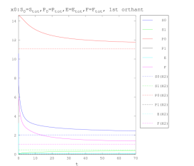
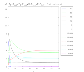
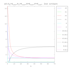
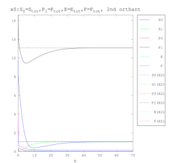
Compute matrices $M^{\bot}$ (or $M$) and $B$ (or $B^{\bot}$) for $G$. Step 1: Compute $\Sigma^{\bot}$ (or any of the sets $\Sigma,\Sigma_{\bot},\Sigma^{\bot}_{\bot}$). Check if $\Sigma^{\bot}$ is mixed. If it is unmixed, stop and assert that the system is monostationary. Step 2: Compute the circuits for $B^{\bot}$ and find an orthant whose support equals the union of the circuits conformal to it. Step 3: For the orthant computed in Step 2, check if there is a conformal circuit of $M$ contained in this orthant. In this case, check whether its support equals the union of the circuits of $M$ conformal to it. Otherwise, ignore it, and go back to Step 2. Step 4: For each orthant $\mathcal{O}$ with $S\cap\mathcal{O}\neq\emptyset$ and $T^{\bot}\cap\mathcal{O}\neq\emptyset$, keep the conformal circuits. Step 5: Build vectors $\mathbf{v}\in T^{\bot}$ and $\mathbf{w}\in S$, for example, as the sum of the corresponding conformal circuits. Step 6: Output $x^{1},x^{2}$ and $\boldsymbol{\kappa}$ that witness multistationarity, as in Theorem 44. Efficiency can certainly be improved at any step of the algorithm, mainly to avoid unnecessary computations. The rows of $M^{\bot}$ usually present some nice structure that minimizes the search for orthants containing a circuit, because in the conditions of Theorem 12 all columns corresponding to the same set in the partition of the species are equal, which produces many zero minors that can be predicted. In Step 5, infinitely many different choices of $\mathbf{v}$ and $\mathbf{w}$ can be obtained by considering positive linear combinations of all circuits which are conformal to the orthant $\mathcal{O}$ (one circuit per support). We implemented this algorithm in Octave [8] for the cascades in Figure 2. In the multistationary case of only one phosphatase $F$, we obtained two different orthants $\mathcal{O}_{1},\mathcal{O}_{2}$ where $S$ and $T^{\bot}$ meet. In both cases, we computed for $i=1,2$ a choice of corresponding rate constants $\boldsymbol{\kappa}(i)$ and two steady states $x^{1}(i)$ and $x^{2}(i)$ in the same stoichiometric compatibility class. We ordered the species $S_{0}$, $S_{1}$, $P_{0}$, $P_{1}$, $ES0$, $FS1$, $S1P0$, $FP1$, $E$, $F$. We considered in both cases two sets of initial conditions (on the same stoichiometric compatibility class); first we set initial states $S_{0}=S_{tot}$, $P_{0}=P_{tot}$, $E=E_{tot}$, $F=F_{tot}$ and then initial states $S_{0}=S_{tot}$, $P_{1}=P_{tot}$, $E=E_{tot}$, $F=F_{tot}$, and all the other species equal to zero. We simulated the system and we depicted the output in Figure 5, which confirms the occurrence of two stoichiometrically compatible steady states for $\boldsymbol{\kappa}(1)$ and $\boldsymbol{\kappa}(2)$. Approximate values are as follows: $$\boldsymbol{\kappa}(1)\cong(25.46,0.86,0.86,11,0.86,0.86,0.14,0.21,0.21,37.47,0.21,0.21),$$ $$x^{1}(1)\cong(0.037,3.47,4.07,1.02,1.16,1.16,4.75,4.75,2.1,0.052),$$ $$x^{2}(1)\cong(2.04,0.47,11.07,0.019,3.16,3.16,1.7,1.75,0.1,1.05),$$ and $$\boldsymbol{\kappa}(2)\cong(101.86,1.72,1.72,33,0.86,0.86,37.47,0.13,0.13,0.42,0.63,0.63),$$ $$x^{1}(2)\cong(0.019,0.052,1.02,4.07,0.58,1.16,7.91,1.58,1.05,1.16),$$ $$x^{2}(2)\cong(1.02,1.05,0.019,11.07,1.58,3.16,2.9,0.58,0.052,0.16).$$ Figure 5. Witnesses for multistationarity of the phosphorylation cascade with one phosphatase $F$, with reaction constants and total amounts obtained from two orthants $\mathcal{O}_{1},\mathcal{O}_{2}$ given by Algorithm 45. Upper plots depict the two different steady states constructed from $\mathcal{O}_{1}$ (dashed lines) along with the simulated trajectories of $S_{0}$, $S_{1}$, $P_{0}$, $P_{1}$, $E$ and $F$. The initial state on the left is $S_{0}=S_{tot}$, $P_{0}=P_{tot}$, $E=E_{tot}$, $F=F_{tot}$, and the initial state on the right is $S_{0}=S_{tot}$, $P_{1}=P_{tot}$, $E=E_{tot}$, $F=F_{tot}$. The lower plots correspond to $\mathcal{O}_{2}$, with the same initial conditions. We used the function ode23s, from the package odepkg version 0.8.5 in Octave [8].

6. Discussion

Our contribution to the study of many different important biological systems modeled with mass-action kinetics is the identification of a common underlying structure in quite diverse networks. We call this a MESSI structure, since it describes Modifications of type Enzyme-Substrate or Swap with Intermediates. The mathematical formulation of the distinguished properties of MESSI biological systems allows us to prove general results on their dynamics from the structure of the network. We give very precise hypotheses that ensure the validity of our statements and which can be easily verified in common networks of biological interest.

It is important to observe that all the conditions and hypotheses in our paper can be algorithmically checked. In particular, it is possible to devise an algorithm to check whether a given network has a MESSI structure, to prove that a given partition is minimal, to construct the associated digraphs and networks, including the corresponding labels, and to check the hypotheses of all our statements. The construction of the rational parametrization in Theorem 28 is also algorithmic. Note also that the sufficient conditions which ensure persistence in Theorem 25 are independent of the conditions to have a toric MESSI system or even an s-toric MESSI system, including the criterion for multistationarity given in Theorem 40. However, the hypotheses in Proposition 42 to ensure the validity of the hypotheses in Theorem 40 also imply persistence. This does not mean that multistationarity is related to persistence, but when there are boundary steady states the hypotheses of Theorem 40 should be verified in an ad hoc manner.

Appendix A Proofs

We assume the reader is familiar with the notion of the Laplacian $\mathcal{L}(G)$ of a digraph $G$ and its main properties. One key observation is that mass-action kinetics associated with a linear digraph $G$ with variables $x=(x_{1},\dots,x_{s})$ equals $\dot{x}=\mathcal{L}(G)x$. A second key observation is that the fact that the rows of $\mathcal{L}(G)$ add up to zero translates into $\sum_{i=1}^{s}\dot{x}_{i}=0$, and so $\sum_{i=1}^{s}x_{i}$ is a conserved quantity. The last key observation is that when $G$ is strongly connected, the kernel of $\mathcal{L}(G)$ has dimension one and there is a known generator $\rho(G)$ with positive entries described as follows. Recall that an $i$-tree $T$ of a graph is a spanning tree where the $i$th vertex is its unique sink (equivalently, the $i$th is the only vertex of the tree with no edges leaving from it), and we call $c^{T}$ the product of the labels of all the edges of $T$. Then, the $i$th coordinate of $\rho(G)$ equals

(14) $$\rho(G)_{i}=\underset{T\;an\;i-tree}{\sum}c^{T}.$$

We refer the reader to [29, 46] for a detailed account.

Conservation Relations and Persistence

In order to prove Theorem 12, we need to first introduce a remark. We call $S_{1}$ the stoichiometric subspace of the biochemical network defined by the associated digraph $G_{1}$ of a MESSI reaction network $G$ (with stoichiometric subspace $S$). We denote by $\tilde{S_{1}}=\{(0,\dots,0,w)\in\mathbb{R}^{p+n}:w\in S_{1}\subseteq\mathbb{R}^{n}\}$ the lifting of $S_{1}$ to $\mathbb{R}^{p+n}$.

Remark 46.

With the previous notation, the following equality of dimensions is an immediate consequence of Lemma 1 in the ESM of [14]:

(15) $$\dim(S)=\dim(S_{1})+p.$$

We will also need Lemma 23 in the main text.

Proof of Lemma 23.

Each vertex in the associated digraph $G_{2}$ to the digraph $G$ is labeled by only one species. If one species of $\mathscr{S}^{(\alpha)}$ appears on a vertex of $G_{2}$, by $({\mathcal{R}}_{2})$ and $({\mathcal{R}}_{3})$ and the construction of $G_{2}$, all the species in the vertices of the corresponding connected component of $G_{2}$ belong to the same $\mathscr{S}^{(\alpha)}$. Moreover, if two core species $X_{i},X_{h}$ in the same subset $\mathscr{S}^{(\alpha)}$ correspond to different connected components of $G_{2}$, then for any complex $y_{ij}$ containing $X_{i}$ and any complex $y_{h\ell}$ containing $X_{h}$, the relation $y_{ij}\rightarrow_{\circ}y_{h\ell}$ does not hold. It follows that we can refine each subset $\mathscr{S}^{(\alpha)}$ as the disjoint union of the subsets of species in each connected component of $G_{2}$ which consists of species in $\mathscr{S}^{(\alpha)}$, and no further refinement is possible if the set of intermediate species is maximal. ∎

We are ready to prove Theorem 12. We will mainly adapt the results in [14] (Theorem 2.1) to our setting.

Proof of Theorem 12.

Given a chemical reaction network $G$ and a partition of the set of species $\mathscr{S}$ that leads to a MESSI system with the given complexes and reactions, consider the mass-action system defined by $G_{1}$, with species $X_{1},\dots,X_{n}$. By Theorem 2.1 in [14], the conservation relations in $G$ are in one-to-one correspondence with the conservation relations of $G_{1}$ in an explicit way that we detail below after our hypotheses. Recall that by Remark 22, the associated graph $G_{2}$ determines the same equations.

Fix $\alpha\geq 1$. As we remarked in the proof of Lemma 23, each subset $\mathscr{S}^{(\alpha)}$ coincides with the variables in the vertices of some of the connected components of the associated digraph $G_{2}$. Given such a connected component $H$, let $\mathscr{S}^{(\alpha)}_{H}$ be its set of vertex labels. As $G_{2}$ is a linear digraph, $H$ is also linear and so the matrix of the associated (linear) system is given by its Laplacian $\mathcal{L}(H)$. Therefore, the sum of its rows equals zero, which means that $\sum_{X_{i}\in S^{(\alpha)}_{H}}\dot{x}_{i}=0$ and a fortiori $\sum_{X_{i}\in S^{(\alpha)}}\dot{x}_{i}=0$, for the mass-action system defined by $G_{1}$. We find now the corresponding linear combination which includes the concentrations of the intermediate species by adapting Lemma 1 in the ESM of [14].

Let $\omega^{\alpha}\in\{0,1\}^{n}$ be the characteristic vector of $\mathscr{S}^{(\alpha)}$, so that $\langle\omega^{\alpha},\dot{x}\rangle=\sum_{X_{i}\in S^{(\alpha)}}\dot{x}_{i}$. For any complex $y^{j}$ of $G_{1}$, we know from $({\mathcal{R}}_{2})$ and $({\mathcal{R}}_{3})$ that it has at most one species in $\mathscr{S}^{(\alpha)}$. Then,

$$\omega^{\alpha}\cdot y^{j}=\left\{\begin{array}[]{ll}1&\text{if there is a species of }\mathscr{S}^{(\alpha)}\text{ in }y^{j}\\ 0&\text{otherwise.}\end{array}\right.$$

Define the $(p+n)$-vector:

$$\widetilde{\omega}^{\alpha}_{i}=\left\{\begin{array}[]{ll}\omega^{\alpha}_{i}&\text{for }i=p+1,\dots,p+n\\ 1&\text{if }i\in\mathrm{Int}(\alpha)\\ 0&\text{otherwise,}\end{array}\right.$$

where $\mathrm{Int}(\alpha)$ is as in (5). Lemma 1 in the ESM of [14] asserts precisely that the linear form defined by $\widetilde{\omega}^{\alpha}$ leads to the conservation of the whole network associated with the linear form defined by $\omega^{\alpha}$ on the variables in $\mathscr{S}_{1}=\mathscr{S}\setminus\mathscr{S}^{(0)}$. But this linear form is precisely $\ell_{\alpha}$, as we wanted to prove. Since we are assuming that all species participate in at least one reaction and intermediate species satisfy condition $(\mathcal{C})$, we have that $\mathscr{S}^{(0)}=\cup_{\alpha=1}^{m}\mathscr{S}\mathrm{Int}(\alpha)$. Therefore, all coefficients of the conservation relation $\sum_{\alpha=1}^{m}\ell_{\alpha}$ are positive and we get that any MESSI system is conservative.

To see the second part of the statement, note that $\ell_{1},\dots,\ell_{m}$ define linearly independent conservation relations and so $\dim(S^{\bot})=s-\dim(S)\geq m$. It only remains to prove that, if $G$ has no swaps, then $s-\dim(S)\leq m$. By Remark 46 it holds that $\dim(S)=\dim(\tilde{S}_{1})+p$ because clearly $\dim(S_{1})=\dim(\tilde{S}_{1})$. It is then enough to show that $\dim(\tilde{S}_{1})\geq n-m$. If $X_{i}+X_{j}\to X_{\ell}+X_{k}$ in $G_{1}$, and there are no swaps in $G$, either $i\in\{\ell,k\}$ or $j\in\{\ell,k\}$. Assume, without loss of generality, that $j=k$. Then $e_{\ell}-e_{i}\in S_{1}$, for $e_{i}$ is the $i$th canonical vector of $\mathbb{R}^{n}$. As $\mathscr{S}$ is minimal, if $X_{i},X_{\ell}\in\mathscr{S}^{(\alpha)}$, necessarily $X_{i}$ and $X_{\ell}$ belong to the same connected component of $G_{2}$. Then there is an undirected path between $X_{i}$ and $X_{\ell}$ in $G_{2}$. By a telescopic sum, as in the proof of Lemma 49 below, we have that each vector $e_{\ell}-e_{i}\in S_{1}$ for each $X_{i},X_{\ell}\in\mathscr{S}^{(\alpha)}$. Fix $X_{i}\in\mathscr{S}^{(\alpha)}$; then for all $\ell\neq i$, $e_{\ell}-e_{i}\in S_{1}$. This gives us $n_{\alpha}-1$ linearly independent vectors for each $\alpha\geq 1$, which are in turn linearly independent from the corresponding vectors obtained from each $\beta$, $\beta\neq\alpha$, $1\leq\beta\leq m$ (when $n_{\alpha}>1$). Adding over $\alpha\geq 1$, we obtain $n-m$ linearly independent vectors in $S$. (Notice that if $\mathscr{S}^{(\alpha)}$ is a singleton, $n_{\alpha}-1=0$.) Therefore, $\dim(S)\geq p+n-m=s-m$, which is what we wanted to prove. The total number of conservation relations in a system is equal to the codimension of the kinetic subspace. If, morover, the kinetic subspace equals $S$, then $\dim(S^{\bot})=m$, as claimed. ∎

We now focus on the occurrence of boundary steady states. Both proofs of Theorem 25 and Proposition 34 below are based on the proof of Theorem 3.1 in [14] (Theorem 2 in their ESM).

Proof of Theorem 25.

Assume there is a boundary steady state in some stoichiometric compatibility class that intersects the positive orthant.

Following the proof of Theorem 2 in the ESM of [14], it can be seen that at steady state the concentration of an intermediate species $u_{k}$ is a nonnegative linear combination of monomials in the concentrations of the core species in the complexes that react via intermediates to it. Then, if there is an intermediate species $U_{k}$ such that $u_{k}=0$ at steady state, there is at least one core species (in a core complex that reacts via intermediates to $U_{k}$) that vanishes at steady state. Therefore, if there is a boundary steady state, there is a core species $X_{i}$ such that $x_{i}=0$ at steady state.

By Lemma 23, we can refine the given MESSI structure in such a way that subsets of core species are in bijection with the connected components of $G_{2}$. In order to avoid unnecessary notation, we will assume in what follows that the partition is minimal. Recall that a vertex in a directed graph has indegree zero if it is not the head of any directed edge. Let us define the subsets of indices

$$L_{0}= \{\beta\geq 1:\text{indegree of }\mathscr{S}^{(\beta)}\text{ is }0\},$$

$$L_{k}= \{\beta\geq 1:\text{for any edge }\mathscr{S}^{(\gamma)}\to\mathscr{S}^{(\beta)}\text{ in }G_{E}\text{ it holds that }\gamma\in L_{t},\text{ with }t<k\}\backslash\underset{t=0}{\overset{k-1}{\bigcup}}L_{t},k\geq 1.$$

The main observation that makes the following inductive argument work is that as $\mathscr{S}$ is finite and there are no directed cycles in $G_{E}$, there must exist a subset $\mathscr{S}^{(\beta)}$ with $1\leq\beta\leq m$ such that its indegree in $G_{E}$ is zero. This means that $L_{0}\neq\emptyset$.

Let $\ell\geq 0$ be minimal with the property that there exist $\alpha\in L_{\ell}$ and a core species $X_{i}\in\mathscr{S}^{(\alpha)}$ such that $x_{i}=0$ at steady state. Denote by $H_{\alpha}$ the connected component of $G_{2}$ with vertices the species in $\mathscr{S}^{(\alpha)}$. Let $\rho(H_{\alpha})$ be the generator of the kernel of $\mathcal{L}(H_{\alpha})$ as in (14). Its entries are nonnegative sums of terms involving the rate constants $\tau$ and concentrations of species in $L_{j}$ with $j<\ell$. Then, $\rho(H_{\alpha})$ has nonzero coordinates since $H_{\alpha}$ is strongly connected because $G_{2}$ is weakly reversible and $\ell$ is minimal. Moreover, the following equation is satisfied at steady state for any $X_{j}\in\mathscr{S}^{(\alpha)}$:

(16) $$\rho(H_{\alpha})_{j}\,x_{i}-\rho(H_{\alpha})_{i}\,x_{j}=0.$$

Then the corresponding concentrations $x_{j}$ vanish at steady state for any $X_{j}\in\mathscr{S}^{(\alpha)}$. Take $k\in\mathrm{Int}(\alpha)$. The concentration of the intermediate species $u_{k}$ is a nonnegative linear combination of monomials in the concentrations of the core species that react via intermediates to it. By condition $(\mathcal{C})$ and rule $({\mathcal{R}}_{3})$, any such monomial contains one variable indexed by a species in $\mathscr{S}^{(\alpha)}$. As $x_{j}=0$ for all $j\in\mathscr{S}^{(\alpha)}$ we get that $u_{k}=0$. This gives a contradiction by (6) in Theorem 12 since $C_{\alpha}$ is a nonzero constant.

As MESSI systems are conservative, the existence of nonnegative steady states is guaranteed by fixed-point arguments. Indeed, a version of the Brouwer fixed-point theorem ensures that a nonnegative steady state exists in each compatibility class. As the system has no boundary steady states, we deduce the existence of a positive steady state in each compatibility class, and, in particular, the consistency of the system. ∎

Parametrizing the steady states

We first prove the existence of rational parametrizations under the hypotheses of Theorem 28.

Proof of Theorem 28.

The arguments of the proof are similar to those in the proof of Theorem 25. Again, we will assume that the partition is minimal to ease the notation. Recall the sets $L_{k}$ in that proof and the crucial remark that $L_{0}\neq\emptyset$ because the graph $G_{E}$ has no directed cycles.

For each $\alpha\geq 1$, fix $X_{i_{\alpha}}\in\mathscr{S}^{(\alpha)}$. Because of the minimality of the partition, any other $X_{i}\in\mathscr{S}^{(\alpha)}$ lies in the connected component $H_{\alpha}$ of $G_{2}$ containing $X_{i_{\alpha}}$. We can then parametrize all the species in $\mathscr{S}^{(\alpha)}$ for $\alpha\in L_{k}$ in terms of $x_{i_{\alpha}}$ and the species in $L_{j}$ for $j<k$, recursively using (16) to write

$$x_{i}=\dfrac{\rho(H_{\alpha})_{i}}{\rho(H_{\alpha})_{i_{\alpha}}}x_{i_{\alpha}}$$

at steady state. Moreover, the concentrations of intermediate species can be rationally written in terms of all $x_{i_{\alpha}},\alpha=1,\dots,m$ (see Definition 18 and Remark 19). Thus, $\dim(V_{f}\cap\mathbb{R}_{>0}^{s})=m$. The last equality $\dim S^{\bot}=m$ in the statement follows from Theorem 12 using Remark 26. ∎

We show now that the positive steady states of s-toric MESSI systems can be described by binomials, and we postpone the proof of the choice of very explicit binomials when any pair of nodes in the same component are connected by a single simple path.

Proof of Proposition 34.

Following the arguments in [14], we first build a new labeled directed graph $\widehat{G}$ with node set $\mathscr{S}^{(0)}\cup\{*\}$, which consists of collapsing all core complexes into the vertex $*$, and labeled directed edges that are obtained from hiding the core complexes in the labels. For example, $X_{i}+X_{j}\overset{\kappa}{\rightarrow}U_{k}$ becomes $*\overset{\kappa x_{i}x_{j}}{\longrightarrow}U_{k}$ and $U_{k}\overset{\kappa^{\prime}}{\rightarrow}X_{i}+X_{j}$ becomes $U_{k}\overset{\kappa^{\prime}}{\longrightarrow}*$. This new graph is linear and satisfies that $\dot{\mathbf{u}}=0$ is equivalent to $\mathcal{L}(\widehat{G})\,\widetilde{\mathbf{u}}=0$, where $\widetilde{\mathbf{u}}=(u_{1},\dots,u_{p},1)^{t}$ (this last coordinate stands for “the concentration” of the node $*$). It is important to notice that the graph $\widehat{G}$ is strongly connected by condition $(\mathcal{C})$.

Then, at steady state we obtain that $\widetilde{\mathbf{u}}$ is proportional to the vector $\rho_{\widetilde{G}}=(\rho_{1},\dots,\rho_{p},\rho)$ defined in (14), so that $u_{k}=\rho_{k}/\rho$ for any $k=1,\dots,p$. It is straightforward to check that every $*$-tree involves labels in $\mathbb{Q}[\kappa]$. On the other hand, for every $U_{k}$, as by condition $(\mathcal{C}^{\prime})$ there is a unique core complex $y_{i_{k}j_{k}}$ such that $y_{i_{k}j_{k}}\rightarrow_{\circ}y_{k}$, every $k$-tree involves labels in $\mathbb{Q}[\kappa,x_{i_{k}}x_{j_{k}}]$. Moreover, as there must be a path from $*$ to $U_{k}$ in each $k$-tree, $x_{i_{k}}x_{j_{k}}$ necessarily appears as a label on those trees. Then,

(17) $$u_{k}=\mu_{k}\,x_{i_{k}}x_{j_{k}},\,k=1,\dots p,$$

where

$$\mu_{k}=\frac{\rho_{k}}{x_{i_{k}}x_{j_{k}}}\frac{1}{\rho}\in\mathbb{Q}(\kappa).$$

∎

Proof of the first part of Theorem 35.

Let $x$ be a positive steady state and $X_{i}\neq X_{j}$ in $\mathscr{S}^{(\alpha)}$ in the same connected component $H$ of $G_{2}$. Let $\rho(H)$ be the explicit generator of the kernel of $\mathcal{L}(H)$ as in (14). Then, as in (16), $\rho(H)_{j}x_{i}-\rho(H)_{i}x_{j}=0$. Fix a $j$-tree $T_{0}$. The product of the labels $c^{T_{0}}$ of all the edges in $T_{0}$ is equal to a monomial $x^{\gamma_{j}}$ times a polynomial in the rate constants $\tau$. For any other $j$-tree $T$, condition ($\mathcal{C}^{\prime\prime\prime}$) ensures that $c^{T}=\mu_{T}(\tau)\,c^{T_{0}}$, with $\mu_{T}\in\mathbb{Q}(\tau)$. It follows that the quotient of the sum $\rho(H)_{j}$ by $x^{\gamma_{j}}$ lies in $\mathbb{Q}(\tau)$ (and also there exists a monomial $x^{\gamma_{i}}$ such that $\rho(H)_{i}/x^{\gamma_{i}}\in\mathbb{Q}(\tau)$). Call

(18) $$\eta_{ij}=\rho(H)_{i}x^{\gamma_{j}}/\rho(H)_{j}x^{\gamma_{i}}\in\mathbb{Q}(\tau)\subset\mathbb{Q}(\boldsymbol{\kappa}).$$

Then, $x^{\gamma_{j}}x_{i}-\eta_{ij}x^{\gamma_{i}}x_{j}=0$. Combining this with (17), the positive steady states can be described by the binomials:

(19) $$u_{k}-\mu_{k}x^{\varphi(k)}\text{ for each intermediate species }U_{k}$$

(20) $$x^{\gamma_{j}}x_{i}-\eta_{ij}x^{\gamma_{i}}x_{j}\text{ if }X_{i},X_{j}\text{ lie in the same connected component of }G_{2}.$$

We can fix one species $X_{i_{h}}$ in each connected component $H$ of $G_{2}$ and consider the binomial equations of the form in (20) where $i=i_{h}$. There are $p$ further binomial equations in (19). These $p+n-m^{\prime}=s-m^{\prime}$ binomial equations cut out the positive steady states. ∎

To prove the second part of Theorem 35, we first need a combinatorial lemma.

Lemma 47.

Assume $H$ is a digraph with the property that there is a unique simple path $P_{ij}$ from any node $X_{i}$ to any node $X_{j}$ in the same connected component of $H$. Then the following hold:

1. For each vertex $X_{i}$ of $H$ there is only one $i$-tree, denoted by $T_{i}$.

2. Let $X_{i}\overset{\tau x_{h}}{\longrightarrow}X_{j}$ be an edge in $H$. Then, $T_{i}$ is obtained from $T_{j}$ by deleting the edge $X_{i}\overset{\tau x_{h}}{\longrightarrow}X_{j}$ and adding the edge $X_{j}\overset{\tau^{\prime}x_{m}}{\longrightarrow}X_{\ell}$, where $X_{\ell}$ is such that $X_{j}\overset{\tau^{\prime}x_{m}}{\longrightarrow}X_{\ell}$ is in $P_{ji}$.

Proof.

Proof of (i): Let $X_{j}$ ($j\neq i$) be in the same connected component of $H$ as $X_{i}$. In any $i$-tree there is an edge leaving from $X_{j}$; otherwise $X_{j}$ would be another sink different from $X_{i}$. Moreover, there must be a path from $X_{j}$ to $X_{i}$ in any such $i$-tree. If the path visits some vertex twice (or more times), there would be a cycle in the underlying undirected graph of the tree, which is not possible. Hence, the path is simple. By hypothesis, there is only one choice for this path, and so there is only one $i$-tree in $H$.

Proof of (ii): Call $T^{\prime}$ the new digraph obtained from $T_{j}$ by deleting the edge $X_{i}\overset{\tau x_{h}}{\longrightarrow}X_{j}$ and adding the edge $X_{j}\overset{\tau^{\prime}x_{m}}{\longrightarrow}X_{\ell}$. $T^{\prime}$ still visits every vertex of the corresponding connected component of $H$, and the only vertex from which no arrows leave is $X_{i}$. We claim that there are no cycles in $T^{\prime}$. In fact, the only possible cycle in $T^{\prime}$ must involve the new edge from $X_{j}$ to $X_{\ell}$. Then, there is a directed path in $T^{\prime}$ (and therefore in $H$) from $X_{\ell}$ to $X_{j}$. Moreover, as the paths in $T_{j}$ are simple, this path from $X_{\ell}$ to $X_{j}$ in $T^{\prime}$ is simple. But in $H$ there is another simple path $P_{\ell i}\cup\{X_{i}\to X_{j}\}$ from $X_{\ell}$ to $X_{j}$, which is different from the one obtained in $T^{\prime}$ since the edge $X_{i}\to X_{j}$ does not exist in $T^{\prime}$. This is a contradiction since by assumption there is only one simple path in $H$ from $X_{\ell}$ to $X_{j}$. Then, $T^{\prime}=T_{i}$. ∎

Proof of the second part of Theorem 35.

If there is a unique simple path $P_{ij}$ from each $X_{i}$ to each $X_{j}$ in the same connected component of $G_{2}$, and $X_{i}\overset{\tau x_{h}}{\longrightarrow}X_{j}$ is in $G_{2}$, the binomial in (19) involves the edges on $T_{i}$ and the edges on $T_{j}$. But, from Lemma 47, $T_{i}$ and $T_{j}$ only differ in the edges $X_{i}\overset{\tau x_{h}}{\longrightarrow}X_{j}$ and $X_{j}\overset{\tau^{\prime}x_{m}}{\longrightarrow}X_{\ell}$, where $X_{\ell}$ is such that $X_{j}\overset{\tau^{\prime}x_{m}}{\longrightarrow}X_{\ell}$ is in $P_{ji}$. Then, after taking out a monomial, the following binomials define the positive steady states:

$$u_{k}-\mu_{k}x^{\varphi(k)}\text{ for each intermediate species }U_{k}$$

$$\tau x_{h}x_{i}-\tau^{\prime}x_{m}x_{j}\text{ if }X_{i}\overset{\tau x_{h}}{\longrightarrow}X_{j}\text{ in }G_{2}^{\circ}\text{ and }X_{j}\overset{\tau^{\prime}x_{m}}{\longrightarrow}X_{\ell}\text{ is in }P_{ji}.$$

∎

Toric MESSI systems and Multistationarity

We will prove Theorem 40 by adapting Proposition 3.9 and Corollary 2.15 in [31] and Theorem 5.5 in [33] to our setting. We recall that a chemical reaction system has the capacity for multistationarity if there exists a choice of rate constants such that there are two or more positive steady states in one stoichiometric compatibility class $(x^{0}+S)\cap\mathbb{R}^{s}_{\geq 0}$ for some initial state $x^{0}\in\mathbb{R}^{s}_{\geq 0}$ (and it is monostationary otherwise).

Remark 48.

Consider a toric MESSI system whose positive steady states can be described by binomial equations of the form $x^{y^{\prime}}-\eta x^{y}=0$. Equivalently, the positive steady states of the toric MESSI system can be described by the monomial equations $x^{y^{\prime}-y}=\eta$, where we consider Laurent monomials. We construct now a matrix $B$ whose columns form a basis of the subspace $T$ generated by these difference vectors $y^{\prime}-y$, and also the monomial map $x\mapsto x^{B}$, where $(x^{B})_{j}=x^{B_{j}}=x_{1}^{B_{1j}}\cdot\ldots\cdot x_{s}^{B_{sj}}$, for each column $B_{j}$ of $B$. Then $x^{*}$ is a positive steady state of the system if and only if ${x^{*}}^{B}=\tilde{\eta}$ for an appropriate vector $\tilde{\eta}$. Thus, the system is monostationary for any choice of rate constants if and only if the monomial map $x\mapsto x^{B}$ is injective on each stoichiometric compatibility class $(x^{0}+S)\cap\mathbb{R}_{>0}^{s}$ for every $x^{0}\in\mathbb{R}_{>0}^{s}$.

Proof of Theorem 40.

Under the hypotheses in the statement, we want to prove the equivalence of the assertions:

1. The associated MESSI system is monostationary.

2. The signs sets $\Sigma,\Sigma^{\bot},\Sigma_{\bot},\Sigma^{\bot}_{\bot}$ are unmixed.

3. For all orthants $\mathcal{O}\in\{-1,0,1\}^{s},\mathcal{O}\neq\mathbf{0}$, either $S\cap\mathcal{O}=\emptyset$ or $T^{\bot}\cap\mathcal{O}=\emptyset$.

We first prove (i) $\Leftrightarrow$ (ii) by adapting the results in [31]. We will see that (i) and (ii) are both equivalent to

$$\{\operatorname{sign}(v):v\in\ker(B^{t})\}\cap\{\operatorname{sign}(v):v\in S\}=\{0\},$$

where $(\operatorname{sign}(v))_{i}=\operatorname{sign}(v_{i})$ for $i=1,\dots,s$. This is also equivalent by the definition of $T^{\bot}$ to

(21) $$\{\operatorname{sign}(v):v\in T^{\bot}\}\cap\{\operatorname{sign}(v):v\in S\}=\{0\}.$$

By Remark 48, (i) is equivalent to the injectivity of the map $x\mapsto x^{B}$ on each stoichiometric compatibility class $(x^{0}+S)\cap\mathbb{R}_{>0}^{s}$. We deduce from Proposition 3.9 in [31] that (i) is equivalent to (21). Previously, in Corollary 2.15 the authors had proved that (21) is in turn equivalent to asking that for all $J\subseteq[s]$, $\#J=s-d=\operatorname{rank}(B)=\operatorname{rank}(M)$, $\det(B_{J})\det(M_{J})$ is either zero or has the same sign as all other nonzero products, and moreover, at least one such product is nonzero. In other words, (21) is equivalent to the set $\Sigma$ being unmixed. By Lemma 39, this is equivalent to (ii). To finish the proof, we just need to show that (21) $\Leftrightarrow$ (iii), but this is straightforward. ∎

We now prove Theorem 44, and we postpone the proof of Proposition 42, which needs an ancillary lemma.

Proof of Theorem 44.

By Theorem 40, if the system is not monostationary, we know that there exists an orthant $\mathcal{O}\in\{-1,0,1\}^{s},\mathcal{O}\neq\mathbf{0}$, such that $S\cap\mathcal{O}\neq\emptyset$ and $T^{\bot}\cap\mathcal{O}\neq\emptyset$. Then, there exist $\mathbf{w}\in S,\mathbf{v}\in T^{\bot}$ such that $\operatorname{sign}(\mathbf{w})=\operatorname{sign}(\mathbf{v})$. Inspired by Theorem 5.5 in [33], for any index $i$ not in the support of $\mathbf{v}$, we choose any positive real number $h_{i}$ and we define positive vectors $x^{1}$ and $x^{2}$ as follows:

$$\left(x^{1}_{i}\right)_{i=1,\,\ldots,\,s}~{} =~{}\left\{\begin{array}[]{lll}\frac{w_{i}}{e^{v_{i}}-1},&&\text{if }v_{i}\neq 0\\ h_{i},&&\text{otherwise,}\end{array}\right.$$

$${x}^{2}~{} =~{}\textrm{diag}(e^{\mathbf{v}})\,{x}^{1}$$

where “$e^{x}$” for a vector $x\in\mathbb{R}_{>0}^{s}$ denotes the vector $(e^{x_{1}},e^{x_{2}},\dots,e^{x_{s}})\in\mathbb{R}^{s}$ and $\mathrm{diag}(x)$ denotes the diagonal matrix whose diagonal is the vector $x$.

As the system is consistent, there exists a positive vector $\lambda$ such that $\sum_{y\to y^{\prime}}\lambda_{yy^{\prime}}(y^{\prime}-y)=0$. For any edge $y\to y^{\prime}$, take the (positive) rate constant

$$k_{yy^{\prime}}=\lambda_{yy^{\prime}}(x^{1})^{-y},$$

which defines a positive vector $\boldsymbol{\kappa}$ satisfying

$$f(x^{1},\boldsymbol{\kappa})=\underset{y\to y^{\prime}}{\sum}\kappa_{yy^{\prime}}\,(x^{1})^{y}\,(y^{\prime}-y)=0.$$

Then, $x^{1}$ is a positive steady state of the system for these reaction rate constants $\boldsymbol{\kappa}$. As the system is a toric MESSI system $x^{1}$ is a solution of the binomial equations that describe the positive steady states. Call $\boldsymbol{\eta}:=(x^{1})^{B}$. Then, $x$ is a positive steady state of the system if and only if $x^{B}=\boldsymbol{\eta}$. It can be checked that $((x^{2})^{B})_{j}=e^{\langle\mathbf{v},B_{j}\rangle}(x^{1})^{B_{j}}$, and, as $\mathbf{v}\in T^{\bot}$, we have $(x^{1})^{B}=(x^{2})^{B}=\boldsymbol{\eta}$. Therefore, $x^{2}$ is also a positive steady state of the system. Moreover, $x^{2}-x^{1}=\mathbf{w}\in S$, and so $x^{1}$ and $x^{2}$ belong to the same stoichiometric compatibility class. ∎

Recall the definitions of $S_{1}$ and $\tilde{S}_{1}$ before Remark 46.

Lemma 49.

Assume that condition $(\mathcal{C}^{\prime})$ in Definition 30 holds, and consider the vectors

(22) $$v_{k}=y_{k}-y_{i_{k}j_{k}}.$$

Then, $S=\tilde{S}_{1}\oplus\langle v_{1},\dots,v_{p}\rangle$.

Proof.

It is clear, from the definitions of $\tilde{S}_{1}$ and the vectors $v_{k}$, that $\tilde{S}_{1}\cap\langle v_{1},\dots,v_{p}\rangle=\{0\}$ (as no intermediate complex appears in the reactions of $G_{1}$). Moreover, the vectors $v_{k}$ are linearly independent, and therefore $\dim(\langle v_{1},\dots,v_{p}\rangle)=p$. By Remark 46, we know that $\dim(S)=\dim(S_{1})+p=\dim(\tilde{S}_{1})+p$. Thus, we only need to show now that $S\supseteq\tilde{S}_{1}\oplus\langle v_{1},\dots,v_{p}\rangle$.

For simplicity, we will assume that all core complexes consist of two species, but it is easy to adapt the proof for the case where the core complexes consist of only one species. We first notice that $v_{k}\in S$ for all $k$. In fact, if $X_{i_{k}}+X_{j_{k}}\rightarrow_{\circ}U_{k}$, there exist $U_{k_{1}},\dots,U_{k_{t}}$ intermediates such that the chain of reactions $X_{i_{k}}+X_{j_{k}}\to U_{k_{1}}\to\dots\to U_{k_{t}}\to U_{k}$ is in $G$. Therefore, from the telescopic sum $y_{k}-y_{i_{k}j_{k}}=(y_{k}-y_{k_{t}})+(y_{k_{t}}-y_{k_{t}-1})+\dots+(y_{k_{2}}-y_{k_{1}})+(y_{k_{1}}-y_{i_{k}j_{k}})$, we see that $v_{k}\in S$, as we wanted to prove. Given $X_{i}+X_{j}\to X_{\ell}+X_{m}$ in $G_{1}$, there exist intermediates $U_{k_{1}},\dots,U_{k_{t}}$ such that the chain of reactions $X_{i}+X_{j}\to U_{k_{1}}\to\dots\to U_{k_{t}}\to X_{\ell}+X_{m}$ is in $G$. As above, from a telescopic sum we deduce that $y_{\ell m}-y_{ij}\in S$. Hence, $\tilde{S}_{1}\subseteq S$ and $\tilde{S}_{1}\oplus\langle v_{1},\dots,v_{p}\rangle\subseteq S$. ∎

Proof of Proposition 42.

By Theorem 28, we know that $\operatorname{rank}(M^{\bot})=m$. We show now that $\operatorname{rank}(B)=s-m$, or equivalently that $\mathrm{dim}(T)=s-m=p+n-m$. From (17) we see that the vectors $v_{k}$ defined in (22) live in $T$ for all $1\leq k\leq p$ (recall that $y_{k}$ denotes the vector corresponding to the monomolecular complex $U_{k}$). This implies that $\langle v_{1},\dots,v_{p}\rangle\subseteq T$. As none of the exponents determined by (19) involves any variable $u_{i}$, it is enough to find $n-m$ linearly independent vectors in $T$ that have support in the last $n$ coordinates.

Call $T_{x}$ the projection $\pi_{x}(T)$ of $T$ onto the last $n$ coordinates corresponding to $x_{1},\dots,x_{n}$. We need to prove then that $\dim(T_{x})=n-m$. For each $\alpha\geq 1$, fix $i_{\alpha}\in\mathscr{S}^{(\alpha)}$ and for each $X_{j}\in\mathscr{S}^{(\alpha)}$, $j\neq i_{\alpha}$, call $z_{i_{\alpha}j}=(\gamma_{j}+e_{i_{\alpha}})-(\gamma_{i_{\alpha}}+e_{j})$, the vector in $\mathbb{R}^{n}$ deduced from the exponents of the binomials in (19). Denote by $T_{\alpha}$ the linear subspace with generators $\{z_{i_{\alpha}j}\}_{j\neq i_{\alpha}}$. We claim that $\dim(T_{\alpha})=n_{\alpha}-1$ for any $\alpha\geq 1$ and that $T_{x}=T_{1}\oplus T_{2}\oplus\dots\oplus T_{m}$

To prove these claims, we need to recall the proof of Theorem 25. We consider again the subsets $L_{0},L_{1},\dots$, and we assume that $\alpha\in L_{k}$. Then, as remarked in the last paragraph of that proof, it holds that the connected component $G_{2}^{\alpha}$ with vertices in $\mathscr{S}^{(\alpha)}$ (ensured by Lemma 23 by our hypothesis of minimality of the partition) has labels in $\mathbb{Q}[\tau,x_{\beta}:\beta\in L_{t},t<k]$. This implies that the $j$th coordinate of the vector $z_{i_{\alpha}h}$ equals $-1$ if $h=j$ and $0$ otherwise. So the vectors $\{z_{i_{\alpha}j}\}_{j\neq i_{\alpha}}$ are linearly independent, that is, $\dim(T_{\alpha})=n_{\alpha}-1$, and by a similar argument we deduce that the sum is direct. Therefore, $\dim(T_{x})=\sum_{\alpha=1}^{m}(n_{\alpha}-1)=n-m$, as wanted.

∎

Algorithm

Step 1 in the algorithm follows directly from Theorem 40. Step 7 follows from [4, 10, 33] and Theorem 44. Theorem 35 explains how to find a matrix $B$ for an s-toric MESSI system. The intermediate steps follow from the following considerations. Given a matrix $A$, every vector in $\mathrm{rowspan}(A)$ is a conformal sum of circuits. (We refer the reader to [30, 36, 43].) Moreover, the circuits of a matrix $A\in\mathbb{R}^{d\times s}$ of rank $d$ are found in the following way. For $J\subseteq[s]$ with $\#J=d-1$, define $r_{J}\in\mathrm{rowspan}(A)$ as the vector $r_{J,\ell}=(-1)^{\mu(\ell,J)}\det(A_{J\cup\{\ell\}})$, where $\mu(\ell,J)$ is the sign of the permutation of $J\cup\{\ell\}$ which takes $\ell$ followed by the ordered elements of $J$ to the ordered elements of $J\cup\{\ell\}$, for all $\ell\in\{0,\dots,s\}$. The following lemma is straightforward and well known.

Lemma 50.

Let $A\in\mathbb{R}^{d\times s}$ be a matrix of rank $d$ and $J\subseteq[s]$ such that $\#J=d-1$ and $\mathrm{rank}(A_{J})=d-1$. Then $r_{J}$ is a circuit of $A$. Moreover, up to a multiplicative constant, these are all the circuits of $A$ (possibly repeated).

Acknowledgments

We would like to thank the referee for providing useful comments.

References

- [1] D. Angeli, P. De Leenher, and E. Sontag, A Petri net approach to the study of persistence in chemical reaction networks, Math. Biosci. 210 (2007), pp. 598 –618.
- [2] A. Björner, M. Las Vergnas, B. Sturmfels, N. White, and G. Ziegler, Oriented matroids, Encyclopedia Math. Appl. 46, 2nd. edition, Cambridge University Press, Cambridge, UK, 1999.
- [3] S. Catozzi. J. P. Di-Bella, A. Ventura, J.-A. Sepulchre, Signaling cascades transmit information downstream and upstream but unlikely simultaneously, BMC Syst. Biol. 16(1) (2016), pp. 1–20.
- [4] C. Conradi, D. Flockerzi, and J. Raisch, Multistationarity in the activation of a MAPK: Parametrizing the relevant region in parameter space, Math. Biosci. 211(1) (2008), pp. 105–131.
- [5] C.Conradi, and A. Shiu, A global convergence result for processive multisite phosphorylation systems, Bull. Math. Biol. 77(1) (2015), pp. 126–155.
- [6] R. J. Davis, Signal transduction by the JNK group of MAP kinases, Cell, 103 (2000), pp. 239–252.
- [7] R. J. Deshaies, and J. E. Ferrell, Multisite phosphorylation and the countdown to S phase, Cell 107(7) (2001), pp. 819–822.
-
[8]
J. W. Eaton, D. Bateman, S. Hauberg, R. Wehbring,
GNU Octave version 4.0.0 manual: a high-level interactive language for
numerical computations,
http://www.gnu.org/software/octave/doc/interpreter/, 2015. - [9] M. Feinberg, Lectures on chemical reaction networks, University of Wisconsin, available at http://crnt.osu.edu/LecturesOnReactionNetworks, 1979.
- [10] M. Feinberg, Multiple steady states for chemical reaction networks of deficiency one, Arch. Ration. Mech. Anal. 132(4) (1995), pp. 371–406.
- [11] M. Feinberg et al., Chemical Reaction Network Toolbox, available at https://crnt.osu.edu/CRNTWin.
- [12] M. Feinberg, F. Horn, Chemical mechanism structure and the coincidence of the stoichiometric and kinetic subspaces, Arch. Ration. Mech. Anal. 66(1) (1977), pp. 83–97.
- [13] E. Feliu, and C. Wiuf, Enzyme-sharing as a cause of multi-stationarity in signalling systems, J. R. Soc. Interface 9(2012), pp. 1224–1232.
- [14] E. Feliu, and C. Wiuf, Simplifying biochemical models with intermediate species, J. R. Soc. Interface, 10 (2013), 20130484.
- [15] E. Feliu, and C. Wiuf, Variable elimination in post-translational modification reaction networks with mass-action kinetics, J. Math. Biol., 66 (2013), pp. 281–310.
- [16] G. Gnacadja,Reachability, persistence, and constructive chemical reaction networks (part II): a formalism for species composition in chemical reaction network theory and application to persistence, J. Math. Chem. 49(10) (2011), pp. 2137–2157.
- [17] G. Gnacadja, Reachability, persistence, and constructive chemical reaction networks (part III): a mathematical formalism for binary enzymatic networks and application to persistence, J. Math. Chem. 49(10) (2011), pp. 2158–2176.
- [18] N. Hermann-Kleiter, and G. Baier, NFAT pulls the strings during CD4+ T helper cell effector functions, Blood 115(15) (2010), pp. 2989–2997.
- [19] P. G. Hogan, L. Chen, J. Nardone, and A. Rao, Transcriptional regulation by calcium, calcineurin, and NFAT, Genes Dev. 17(18) (2003), pp. 2205–2232.
- [20] J. J. Hornberg, B. Binder, F. J. Bruggeman, B. Schoeber, R. Heinrich, and H. V. Westerhoff, Control of MAPK signalling: from complexity to what really matters, Oncogene 24 (2005), pp. 5533–5542.
- [21] W. Hsing, and T. J. Silhavy, Function of conserved histidine-243 in phosphatase activity of EnvZ, the sensor for porin osmoregulation in Escherichia coli, J. Bacteriol. 179 (1997), pp. 3729–3735.
- [22] C.-Y. F. Huang, and J. E. Ferrell, Ultrasensitivity in the mitogen-activated protein kinase cascade, Proc. Natl. Acad. Sci. USA 93(19) (1996), pp. 10078–10083.
- [23] M. M. Igo, A. J. Ninfa, J. B. Stock, and T. J. Silhavy, Phosphorylation and dephosphorylation of a bacterial transcriptional activator by a transmembrane receptor, Genes Dev. 3 (1989), pp. 1725–1734.
- [24] B. N. Kholodenko, Negative feedback and ultrasensitivity can bring about oscillations in the mitogen-activated protein kinase cascades, Eur. J. Biochem., 267 (2000), pp. 1583–1588.
- [25] J. M Kyriakis, and J. Avruch, Mammalian mitogen-activated protein kinase signal transduction pathways activated by stress and inflammation, Physiol. Rev., 81(2) (2001), pp. 807–869.
- [26] F. Macian, NFAT proteins: key regulators of T-cell development and function, Nat. Rev. Immunol. 5(6) (2005), pp. 472–484.
- [27] M. Marcondes de Freitas, E. Feliu, and C. Wiuf, Intermediates, catalysts, persistence, and boundary steady states, J. Math. Biol., 74 (2017) pp. 887–932.
- [28] N. I. Markevich, J. B. Hoek, and B. N. Kholodenko, Signaling switches and bistability arising from multisite phosphorylation in protein kinase cascades, J. Cell Biol. 164 (2004), pp. 353–359.
- [29] I. Mirzaev, J. Gunawardena, Laplacian dynamics on general graphs, Bull. Math. Biol., 75 (2013), pp. 2118–2149.
- [30] S. Müller, G. Regensburger, Elementary vectors and conformal sums in polyhedral geometry and their relevance for metabolic pathway analysis, Front Genet. 7 (2016), p. 90.
- [31] S. Müller, E. Feliu, G. Regensburger, C. Conradi, A. Shiu, A. Dickenstein, Sign conditions for injectivity of generalized polynomial maps with applications to chemical reaction networks and real algebraic geometry, Found. Comput. Math. 16(1) (2016), pp. 69–97.
- [32] G. Pearson, F. Robinson, T. Beers Gibson, B. E. Xu, M. Karandikar, K. Berman, and M. H. Cobb, Mitogen-activated protein (MAP) kinase pathways: regulation and physiological functions, Endocr. Rev., 22 (2001), pp. 153–183.
- [33] M. Pérez Millán, A. Dickenstein, A. Shiu, and C. Conradi, Chemical reaction systems with toric steady states, Bull. Math. Biol. 74(5) (2012), pp. 1027–1065.
- [34] L. Pratt, and T. J. Silhavy, Porin regulation of Escherichia coli, in Two-Component Signal Transduction, J. A. Hoch and T. J. Silhavy, Eds. (American Society for Microbiology, Washington, DC, 1995), pp. 105–127.
- [35] J. Richter-Gebert, and G. M. Ziegler, Oriented matroids, in Handbook of Discrete and Computational Geometry, J. E. Goodman and J. O’Rourke, eds. Chapman and Hall/CRC, Boca Raton, FL, 1997, pp. 111–132.
- [36] R. T. Rockafellar, The elementary vectors of a subspace of , in Combinatorial Mathematics and its Applications (Proc. Conf., Univ. North Carolina, Chapel Hill, N.C., 1967), 104–127. Univ. North Carolina Press, Chapel Hill, N.C., 1969.
- [37] M. Sáez, C. Wiuf, E. Feliu, Graphical reduction of reaction networks by linear elimination of species, J. Math. Biol. 74(1) (2017), pp. 195–237.
- [38] H. J. Schaeffer, and M. J. Weber, Mitogen-activated protein kinases: specific messages from ubiquitous messengers, Mol. Cell Biol. 19 (1999), pp. 2435–2444.
- [39] B. Schoeberl, C. Eichler-Jonsson, E. D. Gilles, and G. Muller, Computational modeling of the dynamics of the MAP kinase cascade activated by surface and internalized EGF receptors, Nat. Biotechnol., 20 (2002), pp. 370–375.
- [40] Y. D. Shaul, and R. Seger, The MEK/ERK cascade: From signaling specificity to diverse functions, Biochim. Biophys. Acta. 1773(8) (2007), pp. 1213–1226.
- [41] G. Shinar, and M. Feinberg, Structural sources of robustness in biochemical reaction networks, Science 327(5971) (2010), pp. 1389–1391.
- [42] A. M. Stock, V. L. Robinson, and P. N. Goudreau, Two-component signal transduction, Annu. Rev. Biochem. 69 (2000), pp. 183–215.
- [43] B. Sturmfels, Gröbner Bases and Convex Polytopes, University Lecture Ser. 8, AMS, Providence, RI, 1995.
- [44] M. Thomson, and J. Gunawardena, The rational parametrisation theorem for multisite post-translational modification systems, J. Theoret. Biol. 261 (2009), pp. 626–636.
- [45] A. Turjanski, J. Vaqué, and J. Gutkind, MAP kinases and the control of nuclear events, Oncogene 26 (2007), pp. 3240–3253.
- [46] W. T. Tutte, W. T., The dissection of equilateral triangles into equilateral triangles, Proc. Cambridge Philos. Soc., 44 (1948), pp. 463–482.
- [47] A. Vol′pert, S. Hudjaev, Analysis in classes of discontinuous functions and equations of mathematical physics, Mech. Anal. 8, Springer, Amsterdam, 1985.
- [48] L. Wang, and E. Sontag, On the number of steady states in a multiple futile cycle, J. Math. Biol. 57(1) (2008), pp. 29–52.
- [49] C. Widmann, S. Gibson, M. B. Jarpe, and G. L. Johnson, Mitogen-activated protein kinase conservation of a three-kinase module from yeast to human, Physiol. Rev., 79 (1999), pp. 143–180.
- [50] T. Zarubin, and J. Han, Activation and signaling of the p38 MAP kinase pathway, Cell Res. 15 (2005), pp. 11–18.
- [51] Y. Zhu, L. Qin, T. Yoshida, and M. Inouye, Phosphatase activity of histidine kinase EnvZ without kinase catalytic domain, Proc. Natl. Acad. Sci. U.S.A. 97 (2000), pp. 7808–7813.