Generalized polarizabilities of the nucleon in baryon chiral perturbation theory

Abstract

The nucleon generalized polarizabilities (GPs), probed in virtual Compton scattering (VCS), describe the spatial distribution of the polarization density in a nucleon. They are accessed experimentally via the process of electron-proton bremsstrahlung ($ep\to ep\gamma$) at electron-beam facilities, such as MIT-Bates, CEBAF (Jefferson Lab), and MAMI (Mainz). We present the calculation of the nucleon GPs and VCS observables at next-to-leading order in baryon chiral perturbation theory (B$\chi$PT), and confront the results with the empirical information. At this order our results are predictions, in the sense that all the parameters are well-known from elsewhere. Within the relatively large uncertainties of our calculation we find good agreement with the experimental observations of VCS and the empirical extractions of the GPs. We find large discrepancies with previous chiral calculations—all done in heavy-baryon $\chi$PT (HB$\chi$PT)—and discuss the differences between B$\chi$PT and HB$\chi$PT responsible for these discrepancies.

I Introduction

Long after the early studies of the electron-proton ($ep$) bremsstrahlung Berg58 ; Berg61 , it was realized that this process holds the key to the generalized polarizabilities (GPs) of the nucleon Guichon:1995pu ; see Ref. Guichon:1998xv for a review. The GPs extend the concept of static polarizabilities to finite momentum-transfer $Q^{2}$, and have an interpretation of the distribution of polarization densities in the nucleon Gorchtein:2009qq . They naturally arise in virtual Compton scattering (VCS) with the incoming virtual photon of spacelike virtuality $Q^{2}$, and the outgoing real photon of very low frequency; hence, the $ep$ bremsstrahlung which, in the one-photon-exchange approximation, decomposes into the Bethe-Heitler (BH) process and VCS, cf. Fig. 1.

Figure 1: Mechanisms contributing to $ep\to ep\gamma$ in the one-photon-exchange approximation: Bethe-Heitler, Born VCS, non-Born VCS. Thick (thin) solid lines denote the proton (the electron), wavy lines denote photons. Small circles denote the interaction vertex of a proton with a virtual photon, and the ellipse stands for the generic non-Born VCS amplitude.

Shown in the figure is also the split of VCS into: A) the Born contribution to VCS, with the intermediate state being the nucleon itself, and B) non-Born contribution to VCS, which at low energies is entirely determined by GPs Guichon:1995pu ; Drechsel:1997xv ; Drechsel:1998zm . The BH and Born VCS contributions are given in terms of the electromagnetic nucleon form factors known from elastic electron scattering. The non-Born VCS amplitude, carrying the information about the “inelastic” structure of the nucleon, is the unknown piece that one is trying to access in the $ep$ bremsstrahlung.

Over the past two decades the experimental studies clearly demonstrated the feasibility of an accurate extraction of proton GPs from $ep$ bremsstrahlung Roche:2000ng ; Bourgeois:2006js ; Bourgeois:2011zz ; d'Hose:2006xz ; Janssens:2008qe ; Doria:2015dyx ; Correa:thesis . This experimental progress has been echoed by theory advances. A number of impressive calculations have been done in heavy-baryon chiral perturbation theory (HB$\chi$PT) Hemmert:1996gr ; Hemmert:1997at ; Hemmert:1999pz ; Kao:2002cn ; Kao:2004us , albeit showing a rather poor convergence. A much more empirically viable theory of proton GPs and VCS was developed by Pasquini et al. Drechsel:2002ar ; Pasquini:2001yy based on fixed-$t$ dispersive relations (DRs) for the VCS amplitudes. Incidentally, this framework is used in many experimental studies to extract the GPs from the VCS observables.

The present work is aiming to advance the chiral effective-field theoretic approach by applying the manifestly Lorentz-invariant variant of baryon chiral perturbation theory (B$\chi$PT) to nucleon VCS and GPs. As many recent calculations demonstrate (see, e.g., Becher:1999he ; Fuchs:2003qc ; Pascalutsa:2004ga ; Holstein:2005db ; Pascalutsa:2005vq ; Ledwig:2011cx ; Alarcon:2011zs ; Alarcon:2012kn ; Yao:2016vbz ; Blin:2016itn ), B$\chi$PT shows an improved convergence over the analogous HB$\chi$PT calculations, and, as result, a more “natural” description of the nucleon polarizabilities and Compton scattering processes Pascalutsa:2004wm ; Hall:2012iw ; Bernard:2012hb ; Lensky:2009uv ; Lensky:2014dda . In this paper, we extend the previous B$\chi$PT calculations of Lensky et al. Lensky:2009uv ; Lensky:2014dda ; Lensky:2015awa , done for nucleon polarizabilities appearing in real and forward doubly-virtual Compton scattering (RCS and VVCS, respectively), to the case of GPs and VCS. As in the previous cases, the present calculation is “predictive” in the sense that it has no free parameters to be fixed by the empirical information from Compton processes. And, as in other cases, we find significant improvements in convergence over the analogous HB$\chi$PT results. Arguably, the main improvement is that our postdictions compare well with the experimental data on VCS observables, at least given the significant theoretical uncertainties.

The paper is organized as follows. In Sec. II, we open with the general remarks concerning the connection between polarizabilities and low-energy Compton scattering processes, and then focus on defining the GPs and the VCS observables. Sec. III contains the details of our B$\chi$PT calculation, including power-counting, diagrams, theory error estimate, and remarks on a number of technical issues which arise in these calculations. Sec. IV compares our calculation with previous estimates: the linear $\sigma$-model, HB$\chi$PT calculations, and fixed-$t$ dispersive estimates. Sec. V confronts the results with the available experimental data. Sec. VI contains the concluding remarks. Appendix A contains expressions for the tensors that are used in the decomposition of the VCS amplitude, whereas Appendix B contains analytic expressions for those combinations of the invariant VCS amplitudes that contribute to the GPs.

II Polarizabilities in Compton processes

Let us start by pointing out that there are two different ways of introducing the momentum-transfer dependence of polarizabilities: one via the forward doubly-virtual Compton scattering (VVCS), the other via the single-virtual Compton scattering (VCS). To see the difference, consider a general Compton scattering (CS) process in Fig. 2, described by a number of scalar amplitudes $A_{i}$, functions of Mandelstam invariants

$$s=(p+q)^{2}=(p^{\prime}+q^{\prime})^{2},\quad t=(q-q^{\prime})^{2}=(p^{\prime}-p)^{2},\quad u=(p-q^{\prime})^{2}=(p^{\prime}-q)^{2}.$$ (1)

The latter satisfy the usual kinematical constraint,

$$s+u+t=2M^{2}+q^{2}+q^{\prime\,2},$$ (2)

with $M$ the nucleon mass and $q^{2}$, $q^{\prime\,2}$ the photon virtualities. The polarizabilities can be equated with the coefficients in the low-energy expansion of the CS amplitudes $A_{i}$. Introducing the invariant energies of the incoming and outgoing photon: $\nu=p\cdot q/M$ and $\nu^{\prime}=p\cdot q^{\prime}/M$, the low-energy expansion requires at least one of them to be small. Note that the kinematical constraint can be written as: $t=-2M\,(\nu-\nu^{\prime})$, hence by energy conservation $t\leq 0$. It is convenient to introduce the kinematic invariant,

$$\xi=\frac{s-u}{4M},$$ (3)

which is odd under the photon crossing, $\xi\to-\xi$, whereas $t$ is even. In the most general situation, the CS amplitudes are functions of four independent variables, e.g., the photon energies and virtualities, $A_{i}=A_{i}(\nu,\nu^{\prime};q^{2},q^{\prime\,2})$, or equivalently, $A_{i}(\xi,t;q^{2},q^{\prime\,2})$.

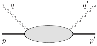
Figure 2: General Compton scattering process. The notation is as in Fig. 1, with the four-momenta of the corresponding particles denoted in the figure.

Now, for real photons ($q^{2}=q^{\prime\,2}=0$), small $\nu$ infers the smallness of $\nu^{\prime}$ and $t$. This is the limit in which the static polarizabilities are defined. For both photons virtual and having the same momentum $q^{\prime}=q$, we deal with the forward VVCS process which, by means of unitarity and causality, can be expressed in terms of nucleon structure functions. In this case the low-energy expansion of the non-Born amplitude is around $\nu=\nu^{\prime}=0$ and the polarizabilities arise as moments of structure functions.

In this work we are concerned with VCS—the Compton process where the initial photon is virtual ($q^{2}=-Q^{2}$) and the final one is real ($q^{\prime\,2}=0$). The polarizabilities are obtained by expanding around $\nu^{\prime}=0$, while $\nu$ is required to be near the lowest physical value (i.e., the elastic threshold): $\nu_{0}=Q^{2}/2M$. This limit corresponds with $t=-Q^{2}$. Note that our $Q^{2}$ corresponds to $\tilde{Q}^{2}$ in the notation of Ref. Guichon:1995pu , and to $Q_{0}^{2}$ in the notation of Ref. Drechsel:1997xv . The three-momentum squared of the initial photon is given in this limit by $\bar{\rm q}^{2}=Q^{2}(1+\tau)$, with $\tau=Q^{2}/4M^{2}=\nu_{0}/2M$.

To distinguish between the GPs arising in VVCS and VCS, we shall refer to the former ones as “symmetric” and to the latter ones as “skewed”. The three considered situations can thus be classified as follows:

static (RCS):

$q^{2}=0$, $q^{\prime\,2}=0$, $\nu\approx 0$, $\nu^{\prime}\approx 0$, $t\approx 0$.

symmetric GPs (VVCS):

$q^{2}=q^{\prime\,2}=-Q^{2}$, $\nu=\nu^{\prime}\approx 0$, $t=0$.

skewed GPs (VCS):

$q^{2}=-Q^{2}$, $q^{\prime\,2}=0$, $\nu^{\prime}\approx 0$, $\nu\approx Q^{2}/2M$, $t\approx-Q^{2}$.

A nice pictorial representation of these situations can be found in Ref. Eichmann:2012mp . Because the low-energy expansions in VVCS and VCS are performed around such different kinematical points, the symmetric and skewed GPs are only connected in the static (real-photon) limit.

Let us now consider the low-energy expansion of VCS in more detail. The low-energy theorem for VCS Guichon:1995pu ; Low:1954kd ; Scherer:1996ux states that the expansion of the non-Born amplitude in powers of the final photon’s energy $\nu^{\prime}$ starts at $O(\nu^{\prime\,1})$, whereas the two leading terms, $O(\nu^{\prime\,-1})$ and $O(\nu^{\prime\,0})$, are entirely determined by the tree-level BH and Born amplitudes. The leading-order [$O(\nu^{\prime\,1})$] non-Born contribution had initially been parametrized by ten skewed GPs Guichon:1995pu . Soon after, it was discovered that the crossing symmetry [see Eq. (6b)] reduces the number of independent GPs to six Drechsel:1997xv . These six GPs are often denoted as

$$P^{(L1,L1)0}(Q^{2}),\ P^{(M1,M1)0}(Q^{2}),\ P^{(L1,L1)1}(Q^{2}),\ P^{(M1,M1)1}(Q^{2}),\ P^{(M1,L2)1}(Q^{2}),\ P^{(L1,M2)1}(Q^{2})\,,$$ (4)

where $P^{(\rho^{\prime}\ell^{\prime},\rho\ell)S}(Q^{2})$ correspond with a multipole amplitude (at $\nu^{\prime}=0$) where $\rho=L,M$ denotes whether the photon is of the longitudinal or the magnetic type and $\ell$ denotes the angular momentum (respectively, $\rho^{\prime}\ell^{\prime}$ or $\rho\ell$ for the final or initial photon); $S=1$ or $S=0$ indicates whether the transition involves the proton’s spin flip or not.

To be more specific, we consider the tensor decomposition of the VCS amplitude $\mathcal{M}^{\mu\nu}$ into the gauge-invariant basis of Ref. Drechsel:1997xv :

$$\mathcal{M}^{\mu\nu}(p^{\prime},q^{\prime},p,q)=\,e^{2}\sum\limits_{i=1}^{12}\rho_{i}^{\mu\nu}A_{i}(\xi,t;q^{2})\,,$$ (5)

where $\mu\ (\nu)$ are the indices of the outgoing (incoming) photon four-vector fields, with tensors $\rho_{i}$ given in Appendix A. The nucleon crossing symmetry in combination with charge conjugation yields the following property of the invariant amplitudes,

$$A_{i}(\xi,t;q^{2}) =+A_{i}(-\xi,t;q^{2}),\quad i=1,2,5,6,7,9,11,12\,,$$ (6a)

$$A_{i}(\xi,t;q^{2}) =-A_{i}(-\xi,t;q^{2}),\quad i=3,4,8,10\,,$$ (6b)

with the latter equation leading to the above-mentioned reduction of the number of independent GPs from 10 to 6. This property is also helpful in checking our loop calculations.

The six GPs of Eq. (4) are defined in terms of the non-Born amplitudes,

$$\bar{A}_{i}(\xi,t;q^{2})\equiv A_{i}(\xi,t;q^{2})-A_{i}^{\mathrm{Born}}(\xi,t;q^{2}),$$ (7)

taken at $\xi=0$ and $t=q^{2}\equiv-Q^{2}$. Introducing a shorthand notation,

$$\bar{A}_{i}(Q^{2})\equiv\bar{A}_{i}(0,\,-Q^{2};-Q^{2}),$$ (8)

the precise expressions for the GPs are given by

$$P^{(L1,L1)0}(Q^{2}) =\hphantom{-}\sqrt{\frac{2}{3}}N_{q}\left[\bar{A}_{1}(Q^{2})+4M^{2}(1+\tau)\bar{A}_{2}(Q^{2})+4M^{2}\tau\left(2\bar{A}_{6}(Q^{2})+\bar{A}_{9}(Q^{2})-\bar{A}_{12}(Q^{2})\right)\right]\,,$$ (9a)

$$P^{(M1,M1)0}(Q^{2}) =-\sqrt{\frac{8}{3}}N_{q}\bar{A}_{1}(Q^{2})\,,$$ (9b)

$$P^{(L1,L1)1}(Q^{2}) =-\frac{2}{3}N_{q}M\tau\left[\bar{A}_{5}(Q^{2})+\bar{A}_{7}(Q^{2})+4\bar{A}_{11}(Q^{2})+4M\bar{A}_{12}(Q^{2})\right]\,,$$ (9c)

$$P^{(M1,M1)1}(Q^{2}) =-\frac{2}{3}N_{q}\frac{M\tau}{1+\tau}\left[\bar{A}_{5}(Q^{2})-2M\tau\bar{A}_{12}(Q^{2})\right]\,,$$ (9d)

$$P^{(M1,L2)1}(Q^{2}) =\hphantom{-}\frac{2}{3}\sqrt{\frac{2}{3}}N_{q}\left[\frac{\tau}{2(1+\tau)}\bar{A}_{5}(Q^{2})+\frac{1}{2}\bar{A}_{7}(Q^{2})+2\bar{A}_{11}(Q^{2})+\frac{M\tau}{1+\tau}\bar{A}_{12}(Q^{2})\right]\,,$$ (9e)

$$P^{(L1,M2)1}(Q^{2}) =-\frac{\sqrt{2}}{6}N_{q}\frac{1}{1+\tau}\left[8M\bar{A}_{6}(Q^{2})+\bar{A}_{7}(Q^{2})+4M\bar{A}_{9}(Q^{2})+4\bar{A}_{11}(Q^{2})+2M\tau\bar{A}_{12}(Q^{2})\right]\,,$$ (9f)

with the normalization factor $N_{q}$ usually taken to be

$$N_{q}=\sqrt{\frac{2M+\nu_{0}}{2(M+\nu_{0})}}=\sqrt{\frac{1+\tau}{1+2\tau}}\,.$$ (10)

At the real-photon point, these GPs relate to the static nucleon polarizabilities Guichon:1995pu ; Drechsel:1998zm :

$$P^{(L1,L1)0}(0) =-\mbox{$\frac{1}{\alpha_{\mathrm{em}}}\sqrt{\frac{2}{3}}$}\,\alpha_{E1}\,,$$ (11a)

$$P^{(M1,M1)0}(0) =-\mbox{$\frac{1}{\alpha_{\mathrm{em}}}\sqrt{\frac{8}{3}}$}\,\beta_{M1}\,,$$ (11b)

$$P^{(M1,L2)0}(0) =-\mbox{$\frac{1}{\alpha_{\mathrm{em}}}\frac{2}{3}\sqrt{\frac{2}{3}}$}\,\gamma_{M1E2}\,,$$ (11c)

$$P^{(L1,M2)0}(0) =-\mbox{$\frac{1}{\alpha_{\mathrm{em}}}\frac{\sqrt{2}}{3}$}\,\gamma_{E1M2}\,,$$ (11d)

where $\alpha_{\mathrm{em}}=e^{2}/4\pi\simeq 1/137$ is the fine structure constant. The remaining two GPs, $P^{(L1,L1)1}$ and $P^{(M1,M1)1}$, vanish (at $Q^{2}=0$). Their slopes, on the other hand, can be related to other static polarizabilities and to “symmetric” GPs via the spin-dependent sum rules Pascalutsa:2014zna ; Hagelstein:2015egb ; Lensky:2017dlc .

The “skewed” generalizations of the electric and magnetic dipole polarizabilities are thus defined as follows:

$$\alpha_{E1}(Q^{2}) =-\alpha_{\mathrm{em}}\mbox{$\sqrt{\frac{3}{2}}$}P^{(L1,L1)0}(Q^{2})\,,$$ (12a)

$$\beta_{M1}(Q^{2}) =-\alpha_{\mathrm{em}}\mbox{$\sqrt{\frac{3}{8}}$}P^{(M1,M1)0}(Q^{2})\,.$$ (12b)

Similar generalizations can be made for the two spin polarizabilities in Eqs. (11c) and (11d).

Finally, let us recall the relation to experimental observables. As noted above, the six GPs of Eq. (4) suffice to fully parametrize the leading (linear in $\nu^{\prime}$) term in the non-Born VCS amplitude. The latter, together with the BH and Born VCS amplitudes, can be used to calculate the observables of $ep$ bremsstrahlung. Most notably, the expression for the unpolarized five-fold differential cross-section can be cast in the following form,

$$\mathrm{d}^{5}\sigma=\mathrm{d}^{5}\sigma^{\mathrm{BH+Born}}+\nu^{\prime}\Phi\left\{V_{1}\left[P_{LL}(Q^{2})-\frac{1}{\varepsilon}P_{TT}(Q^{2})\right]+V_{2}\sqrt{\varepsilon(1+\varepsilon)}P_{LT}(Q^{2})\right\}\,,$$ (13)

where $\Phi$, $V_{1}$, and $V_{2}$ are kinematical factors (see Ref. Guichon:1995pu for the specific expressions thereof), $\varepsilon$ is the electron polarization transfer parameter, $P_{LL}$, $P_{TT}$, and $P_{LT}$ are the VCS response functions given in terms of GPs as follows Guichon:1998xv :

$$P_{LL}(Q^{2}) =-2\sqrt{6}MG_{E}(Q^{2})P^{(L1,L1)0}(Q^{2})\,,$$ (14a)

$$P_{TT}(Q^{2}) =\hphantom{-}6MG_{M}(Q^{2})(1+\tau)\left[2\sqrt{2}\,M\tau\,P^{(L1,M2)1}(Q^{2})+P^{(M1,M1)1}(Q^{2})\right]\,,$$ (14b)

$$P_{LT}(Q^{2}) =\hphantom{-}\sqrt{\mbox{$\frac{3}{2}$}}M\sqrt{1+\tau}\left[G_{E}(Q^{2})P^{(M1,M1)0}(Q^{2})-\sqrt{6}\,G_{M}(Q^{2})P^{(L1,L1)1}(Q^{2})\right]\,,$$ (14c)

where $G_{E}(Q^{2})$ and $G_{M}(Q^{2})$ are the Sachs electric and magnetic form factors of the nucleon.

The unpolarized differential cross-section thus gives information about two linear combinations of the VCS response functions: $\displaystyle P_{LL}-P_{TT}/\varepsilon$ and $P_{LT}$. These two quantities are dominated by the scalar GPs: $P^{(L1,L1)0}$ and $P^{(M1,M1)0}$. Note, however, that performing unpolarized VCS experiments at fixed $Q^{2}$ and for two different values of $\varepsilon$ allows to separate $P_{LL}$ and $P_{TT}$ and thus to access one combination of spin GPs, $P_{TT}$. To obtain information on all spin GPs, one needs to consider polarization observables. We will be interested, in particular, in the response function Vanderhaeghen:1997bx

$$P^{\perp}_{LT}(Q^{2})=\frac{M}{Q}\frac{G_{E}(Q^{2})}{G_{M}(Q^{2})}P_{TT}(Q^{2})-\frac{Q}{4M}\frac{G_{M}(Q^{2})}{G_{E}(Q^{2})}P_{LL}(Q^{2})$$ (15)

which has been accessed experimentally using the beam-recoil polarization asymmetries Doria:2015dyx .

III Chiral perturbation theory of generalized polarizabilities

Our aim is to compute the nucleon VCS amplitudes $A_{i}(\xi,t;q^{2})$ and subsequently the “skewed” GPs using the SU(2) chiral perturbation theory ($\chi$PT) Weinberg:1978kz ; Gasser:1983yg , including the nucleon and $\Delta(1232)$ degrees of freedom. We shall employ B$\chi$PT which is the manifestly-covariant extension of $\chi$PT to the single-baryon sector in its most straightforward implementation (i.e., not the “infrared regularization” of Ref. Becher:1999he ), where the nucleon is included as in Ref. Gasser:1987rb , and the $\Delta(1232)$ as in Ref. Pascalutsa:2006up , see also Geng:2013xn for concise overview. The heavy-baryon results can easily be obtained from B$\chi$PT by an additional expansion in the inverse powers of baryon masses.

III.1 Further remarks on power counting

Let us recall that the chiral effective-field theory is based on the perturbative expansion in powers of pion momentum $p$ and mass $m_{\pi}$ over the scale of spontaneous chiral symmetry breaking $\Lambda_{\chi}\sim 4\pi f_{\pi}$, with $f_{\pi}\simeq 92$ MeV the pion decay constant. Each operator in the effective Lagrangian, or a graph in the loopwise expansion of the S-matrix, can be assigned with an order of $p$. To give a relevant example consider the operator

$$\bar{N}NF^{2},$$ (16)

with $N(x)$ standing for the Dirac field of the nucleon, and $F^{2}$ is the square of the electromagnetic field tensor, $F_{\mu\nu}(x)=\partial_{[\mu}A_{\nu]}(x)$. This is an operator of $O(p^{4})$, since two of the $p$’s come from the photon momenta which are supposed to be small, and the other two powers arise because the two-photon coupling to the nucleon must carry a factor of $\alpha_{\mathrm{em}}$ (the charge $e$ counts as $p$, as we want the derivative of the pion field to count as $p$ even after including the minimal coupling to the photon).

This operator enters the effective Lagrangian with a so-called low-energy constant (LEC), denoted by $C$, and it gives a contribution to the Compton scattering amplitude in the form of

$$\mathcal{M}^{\mu\nu}_{C}=C\,(q\cdot q^{\prime}\,g^{\mu\nu}-q^{\mu}q^{\prime\,\nu}),$$ (17)

hence leading to a shift in the magnetic dipole polarizability: $\beta_{M1}\to\beta_{M1}+C/4\pi$. Now, two important remarks are in order.

• Naturalness. The value of $C$ is not completely arbitrary, but should rather go as $C=(e^{2}/{\Lambda}_{\chi}^{3})c$, with the dimensional constant $c$ being of order of 1, or more precisely:

  $$p/{\Lambda}_{\chi}\ll|c|\ll{\Lambda}_{\chi}/p\,.$$ (18)

  This condition ensures that the contribution of this operator is indeed of $O(p^{4})$, as the power counting commands.

• Predictive powers. This LEC enters very prominently in Compton scattering and polarizabilities—at the tree level, which means its value is best fixed by the empirical information on these quantities. If this is so, the $O(p^{4})$ is not “predictive”, as it could only be used to fit the $\chi$PT result to experiment or lattice QCD calculations. On the other hand, contributions of orders lower than $p^{4}$ are predictive, as they only contain LECs fixed from elsewhere. It is crucial to first study the predictive contributions, if there are any, and this is what we shall focus on here, for the case of VCS and GPs.

The “predictive” contributions to Compton scattering and polarizabilities had been identified in Ref. Lensky:2009uv and computed for the case of real-Compton scattering therein and for VVCS in Lensky:2014dda . Our present calculation of VCS is quite analogous to those works and hence we refer to them for most of the technical details, such as the expressions for the relevant terms of the effective Lagrangian.

On the conceptual side, it is important to note that the counting of the $\Delta(1232)$ effects is done in the so-called “$\delta$-counting” Pascalutsa:2002pi . In it, the Delta-nucleon mass difference $\varDelta=M_{\Delta}-M$ is counted as a light scale ($\varDelta\ll{\Lambda}_{\chi}$) which is substantially heavier than the pion mass ($m_{\pi}\ll\varDelta)$. Hence, if $p\sim m_{\pi}$, then $O(p^{4}/\varDelta)$ is in between of $O(p^{3})$ and $O(p^{4})$.

For the non-Born VCS amplitude and polarizabilities the predictive orders are $O(p^{3})$ and $O(p^{4}/\varDelta)$. The $O(p^{3})$ contribution comes from the pion-nucleon loops shown in Fig. 3. We refer to it here as the leading-order (LO) contribution. The $O(p^{4}/\varDelta)$ contribution, arising at the next-to-leading order (NLO), comes from the Delta pole graph and the pion-Delta loops shown in Fig. 4.

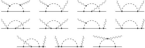
Figure 3: Pion-nucleon loops of $O(p^{3})$. Solid (dashed) lines denote nucleons (pions). Crossed and time-reversed graphs are not shown but are included in the calculation.

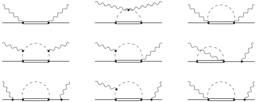
Figure 4: Pion-Delta loops and the Delta tree of $O(p^{4}/\varDelta)$ (in the low-energy regime). Crossed and time-reversed graphs are not shown but are included in the calculation. Double lines denote the propagator of the Delta.

Going into further detail, we note that the feature of the $\delta$-counting is that the characteristic momentum $p$ distinguishes two regimes: low-energy ($p\simeq m_{\pi}$), and resonance ($p\simeq\varDelta$). The above counting is limited to the low-energy regime. Since we are interested in the VCS amplitude at the specific kinematics point where the GPs are defined (i.e., $\xi=0$, $t=-Q^{2}$), we do not consider the regime where one-Delta-reducible graphs are enhanced (resonance regime). However, going to higher $Q$ one does need to count the Delta propagators similar to the nucleon propagators, which, in turn, calls for inclusion of pion-Delta loops with two and three Delta propagators, which have been omitted here. They are only included implicitly to restore current conservation by adjusting the isospin coefficients of one-nucleon-reducible graphs in Fig. 4, as explained in Ref. Lensky:2009uv . Apart from that, pion-Delta loops have rather mild dependence on momenta and the missing loops are unlikely to significantly affect the $Q^{2}$-dependence of the GPs, even for $Q^{2}$ comparable to $\varDelta^{2}$.

To conclude this section, a remark is in order about the $\pi^{0}$ anomaly graph, sometimes considered to be a part of the Born contribution. It enters the VCS amplitude at $O(p^{2})$ and represents the dominant part of the spin GPs (all except $P^{(L1,L1)1}$ where it does not enter). However, the anomaly contributions cancel in the response functions introduced above. We will also omit them when showing results for the spin GPs.

III.2 In practice

The calculation of the $\pi N$ and $\pi\Delta$ loop graphs in Fig. 3 and 4 is analogous to Ref. Lensky:2009uv , with the obvious extension to the case of finite virtuality of the initial photon. The renormalization is done in the exactly the same way; namely, graphs with the nucleon self-energy and with the one-loop $\gamma NN$ vertices are subtracted according to the usual prescription

$$\Sigma_{R}(\not{p}_{s}) =\Sigma(\not{p}_{s})-\Sigma(\not{p})-\Sigma^{\prime}(\not{p})(\not{p}_{s}-M)\,,$$ (19)

$$\Gamma^{\mu}_{R}(p,p^{\prime}) =\Gamma^{\mu}(p,p^{\prime})-\Big{[}\gamma^{\mu}F_{1}(q^{2})-\frac{1}{2M}\gamma^{\mu\nu}q_{\nu}F_{2}(q^{2})\Big{]}\,,$$ (20)

where $p_{s}$ and $p$ in the first equation are the off-shell and the on-shell momentum of the nucleon, whereas $F_{1}(q^{2})$ and $F_{2}(q^{2})$ are the on-shell nucleon Dirac and Pauli form factors resulting from the unsubtracted $\gamma NN$ vertex $\Gamma^{\mu}(p,p^{\prime})$, with $q=p^{\prime}-p$ being the momentum transfer from the photon to the nucleon.

The Delta pole graph in Fig. 4 is calculated in Refs. Lensky:2014dda ; Pascalutsa:2005vq , and as in those works the magnetic $\gamma N\Delta$ coupling $g_{M}$ acquires the dipole behavior that mimics the form expected from vector-meson dominance:

$$g_{M}\to\frac{g_{M}}{\big{[}1+\left(Q/\Lambda\right)^{2}\big{]}^{2}}\,,$$ (21)

with the dipole mass $\Lambda^{2}=0.71$ GeV².

Concerning the implementation of tensor decomposition in Eq. (5), it proved to be useful to write the basis tensors $\rho_{i}$, $i=1,\dots,12$, in terms of the Tarrach tensors $T_{i}$, $i=1,\dots,34$, introduced for the most general VVCS case Tarrach:1975tu , see Appendix A. All tensors $\rho_{i}$, apart from $\rho_{2}$, $\rho_{3}$, and $\rho_{6}$, have unique structures that allow for unambiguous identification of the corresponding parts of the amplitude, e.g., the combination $T_{29}+T_{30}$ enters only $\rho_{12}$, $T_{17}$ enters only $\rho_{11}$, and so on. After the tensors $\rho_{i}$, $i\neq 2,3,6$, have been identified, the remaining tensors can be identified as well, since at this stage they are the only ones that can enter the rest of the amplitude. Since the basis $\rho_{i}$ is explicitly gauge invariant, all the terms that are not proportional to any of $\rho_{i}$ have to vanish when one decomposes a gauge invariant amplitude, e.g., summing up a gauge invariant subset of Feynman graphs such as the $\pi N$ loops in Fig. 3 with their crossed and time-reversed partners, or the Delta pole graph in Fig. 4 with its crossed partner, or the $\pi\Delta$ loops in that figure with their crossed and time-reversed partners. Ensuring that the rest of the amplitude vanishes after the terms proportional to $\rho_{i}$ have been subtracted represents a non-trivial check of a VCS calculation.

We note as well that the tensor decomposition introduces false singularities in the amplitudes due to some of the coefficients in front of $T_{i}$ proportional to $\xi$; these singularities disappear in the end, which serves as yet another check of the calculation. These singularities tend to interfere with the false on-shell singularities in one-nucleon-reducible graphs, i.e., graphs with the nucleon self-energy loop and those with the one-loop $\gamma NN$ vertices. These latter singularities also have to disappear in the end since both the self-energy and the one-loop $\gamma NN$ vertices are subtracted on-shell, as explained above.

It is more convenient, however, to explicitly remove on-shell singularities from the integrals over the Feynman parameters; this can be done by integrating by parts in these integrals and by additional subtractions where they are needed. To illustrate these techniques, we give two examples of typical terms arising in the $\pi N$ self-energy graph, where the on-shell singularities are manifest:

$$\text{A)}\ X_{1} =\frac{1}{\bar{s}-1}\int\limits_{0}^{1}\mathrm{d}x\left\{\log\left[x^{2}+\mu^{2}(1-x)-(\bar{s}-1)x(1-x)\right]-\log\left[x^{2}+\mu^{2}(1-x)\right]\right\}\,,$$ (22)

$$\text{B)}\ X_{2} =\frac{1}{\bar{s}-1}\int\limits_{0}^{1}\mathrm{d}x\frac{x^{2}\left[x^{2}(2x-1)-3\mu^{2}(x-1)^{2}+2(\bar{s}-1)x(x-1)^{2}\right]}{\left[x^{2}+\mu^{2}(1-x)\right]\left[x^{2}+\mu^{2}(1-x)-(\bar{s}-1)x(1-x)\right]}\,,$$ (23)

here $\mu=m_{\pi}/M$ and $\bar{s}=s/M^{2}$. The singularity at $\bar{s}\to 1$ appearing in $X_{1}$ is cancelled when one integrates by parts in the first integral, whereas in order to deal with $X_{2}$ one notices that the integral in it vanishes at $\bar{s}\to 1$. This means that the integrand of $X_{2}$ can be subtracted at $\bar{s}=1$; the singularity cancels after this subtraction.

Removing the on-shell false singularities explicitly allows one to deal with the remaining $1/\xi$ false singularities that come from the tensor decomposition by simply expanding the integrals in powers of $\xi$. It appears to be possible to analytically verify that coefficients in front of negative powers of $\xi$ turn to zero after integration over the Feynman parameters, both for the $\pi N$ and $\pi\Delta$ loops.

Given the kinematics of VCS, one is only interested in the $\xi^{0}$ term in the expansion of the thus obtained amplitudes $A_{i}(\xi,t;q^{2})$, while the Mandelstam variable $t$ is also set to $t=q^{2}\equiv-Q^{2}$. The resulting functions $\bar{A}_{i}(Q^{2})$ are obtained as integrals over two Feynman parameters; an expansion in $Q^{2}$ around the static point $Q^{2}=0$ allows for the integrals to be taken analytically. Appendix B contains expressions for those linear combinations of $\bar{A}_{i}(Q^{2})$ that enter the GPs given by Eq. 4, resulting from the $\pi N$ loop graphs in Fig. 3 and from the Delta pole graph in Fig. 4. The corresponding expressions for the $\pi\Delta$ loops in Fig. 4 are given in the supplementary material to this article.

III.3 Error estimate

In making comparison with experimental data, it is important to provide a theoretical uncertainty. In the case of an EFT expansion, the common way to obtain this uncertainty is via the estimate of higher-order contributions. This work employs the following estimate. In the low-momenta regime, where the expansion parameter is $\displaystyle\delta\sim p/\varDelta$, our calculation is of the next-to-leading order (NLO). A conservative estimate of the next-to-next-to-leading order (NNLO) contributions would be $\text{error}(f)=\delta^{2}f$, where $f$ is a generic VCS amplitude or response function. It is important to note, however, that the error of the scalar polarizabilities $\alpha_{E1}(Q^{2})$ and $\beta_{M1}(Q^{2})$ in the static limit $Q^{2}=0$ is defined by the error of the corresponding static (real) polarizabilities. This error was argued to be small Lensky:2015awa due to the fact that these polarizabilities are very close at NLO to the results obtained in B$\chi$PT fits to real Compton scattering data Lensky:2014efa , and that there are contact terms at NNLO that will in any case compensate changes in $\alpha_{E1}$ and $\beta_{M1}$ coming from other higher-order mechanisms. The static errors are estimated as $\text{error}(\alpha_{E1},\text{static})\simeq\text{error}(\beta_{M1},\text{static})\sim 0.7\times 10^{-4}$ fm³ (see Ref. Lensky:2015awa ); this translates to the uncertainty of $4.7$ GeV² and $2.3$ GeV² in $P_{LL}(0)$ and $P_{LT}(0)$, respectively. This static uncertainty has to dominate at very small $Q^{2}$, whereas at larger $Q^{2}$ (still in the low-momenta regime) the term $\delta^{2}f\sim(p^{2}/\varDelta^{2})f$ will become more important. In practice, we take the sum of the two values.

The uncertainty estimate in the high-momenta regime works in a similar way. In this regime, $p\gtrsim\varDelta$, our calculation is at an incomplete leading order (LO), however, we will treat it as an LO calculation as argued above. The expansion parameter in this regime can be one of these,

$$\delta=\left\{\frac{m_{\pi}}{\varDelta},\frac{p}{\Lambda_{\chi}},\frac{\varDelta}{\Lambda_{\chi}}\right\}\,,$$

and we take the average value of the three in order to estimate the NLO contribution. In summary, our uncertainty estimate for a VCS amplitude or a response function $f$ is given by

$$\text{error}(f)=\left\{\begin{matrix}\text{error}(f,\text{static})+\displaystyle\frac{p^{2}}{\varDelta^{2}}f\,,&p\lesssim\varDelta\,,\\ &\\ \displaystyle\frac{1}{3}\left(\frac{m_{\pi}}{\varDelta}+\frac{p}{\Lambda_{\chi}}+\frac{\varDelta}{\Lambda_{\chi}}\right)f\,,&p\gtrsim\varDelta\,,\end{matrix}\right.$$ (24)

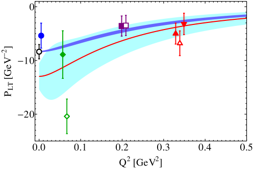
Figure 8: VCS response function $P_{LT}(Q^{2})$. Notation is as in Fig. 7.

where $\text{error}(f,\text{static})$ is the static uncertainty discussed above. To obtain smooth bands in the plots, the uncertainties in the different regimes are multiplied by smooth transition functions. One has to note that this error estimate can lead to artifacts such as zero crossings, in the regime $p\gtrsim\varDelta$: the error being proportional to the observable, it can become small or even turn to zero if the latter decreases or vanishes. While we still consider this issue to be tolerable as far as the plots we demonstrate here are concerned, one can see it manifest, for instance, in Figs. 8 and 11 below, where the bands of $P_{LT}$ and $\beta_{M1}$ shrink at larger values of $Q^{2}$.

IV Comparison with previous calculations

In this section, we compare our B$\chi$PT results with previous results obtained in HB$\chi$PT, in the linear sigma model, and with fixed-$t$ dispersion relations. Matching our results against those obtained in the former two frameworks provides an important check of our calculation.

IV.1 Linear $\sigma$-model

The first check is made by comparing our results with the results of Metz and Drechsel Metz:1996fn ; Metz:1997fr who calculated the nucleon GPs in the linear sigma model at one-loop level. Their linear sigma model calculation, performed in the limit of infinitely large sigma meson mass, is exactly equivalent to the $O(p^{3})$ one-loop pion-nucleon B$\chi$PT result. The easiest way to see it is perhaps to compare the Lagrangian used in Refs. Metz:1996fn ; Metz:1997fr with the B$\chi$PT Lagrangian after the field redefinition done in Ref. Lensky:2009uv . Metz and Drechsel provide only the expressions at $Q^{2}=0$ for the GPs and their derivatives. They also give second derivatives for the two spin-dependent GPs that vanish at $Q^{2}=0$. The expressions for all of the spin-dependent GPs are in addition expanded in $1/M$ up to NNLO. Our calculation has been able to reproduces all of their results except one: their expression for $\alpha_{E1}$ of the proton, which we believe to be due to a typo in the second line of Eq. (17) of Ref. Metz:1996fn , namely, the first term in the square brackets should read $152$ instead of $157$.

IV.2 Heavy-baryon expansion

By expanding our results in powers of $1/M$ we can check against the HB$\chi$PT calculation of Hemmert et al. Hemmert:1999pz that includes the Delta isobar in the $\epsilon$-expansion Hemmert:1996xg . We checked that the leading term of the heavy-baryon expansion of our results for the scalar GPs (with the $\pi N$ and $\pi\Delta$ loops corresponding to, respectively, $O(p^{3})$ and $O(\epsilon^{3})$ result of Hemmert et al.) reproduces the results of Ref. Hemmert:1999pz .

The spin-dependent GPs have also been calculated in HB$\chi$PT without the Delta isobar up to incomplete $O(p^{5})$ in Refs. Kao:2002cn ; Kao:2004us . These calculations include $\pi N$ loops with photon couplings to the anomalous magnetic moment (a.m.m.) of the nucleon inside the loop, which appear at $O(p^{4})$ and are not included in our calculation. Nevertheless, the heavy-baryon expansion of our results should reproduce their HB$\chi$PT expressions, once the a.m.m. couplings are set to zero. We have reproduced the HB$\chi$PT expressions for $P^{(M1,M1)1}$ and $P^{(L1,M2)1}$, calculated in Ref. Kao:2004us . The other two spin-dependent GPs, $P^{(L1,L1)1}$ and $P^{(M1,L2)1}$, are reproducible up to the leading order in $1/M$; the differences at NLO start in the second non-vanishing terms in the expansion in powers of $Q^{2}$, i.e., the first derivative of $P^{(M1,L2)1}$ with respect to $Q^{2}$, and in the second derivative of $P^{(L1,L1)1}$.

Is is important to realize that $P^{(L1,L1)1}$ and $P^{(M1,L2)1}$ at $O(p^{5})$ were deduced in Ref. Kao:2004us by using the nucleon crossing relations of Eq. (6b), which in HB$\chi$PT do not hold exactly due to the lack of an exact charge conjugation symmetry. The mismatch between the HB results and ours demonstrates that these crossing relations should not be used in HB$\chi$PT to obtain complete expressions for the terms of higher-order in $1/M$ expansion.

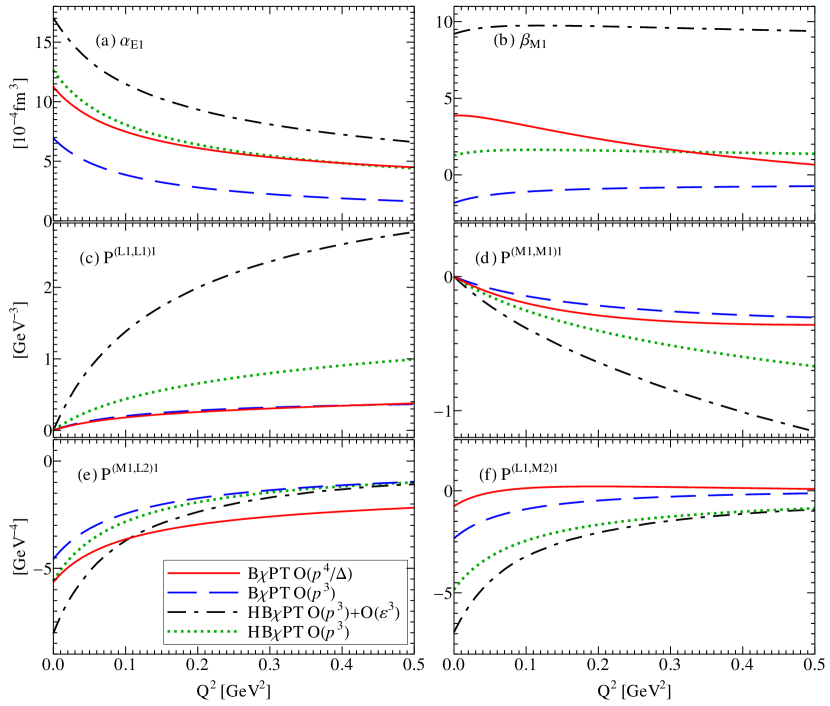
Figure 5: Comparison of covariant B$\chi$PT and HB$\chi$PT results for generalized polarizabilities: (a) $\alpha_{E1}(Q^{2})$; (b) $\beta_{M1}(Q^{2})$; (c) $P^{(L1,L1)1}(Q^{2})$; (d) $P^{(M1,M1)1}(Q^{2})$; (e) $P^{(M1,L2)1}(Q^{2})$; (f) $P^{(L1,M2)1}(Q^{2})$. Red solid curve: covariant $O(p^{3})+O(p^{4}/\varDelta)$; blue dashed curve: covariant $O(p^{3})$; black dot-dashed curve: HB $O(p^{3})+O(\epsilon^{3})$; green dotted curve: HB $O(p^{3})$. HB results are from Refs. Hemmert:1999pz ; Kao:2004us .

For completeness, we provide here our results for the HB expansion of the spin GPs up to NLO in $1/M$. The LO results are the same as given in Refs. Hemmert:1999pz ; Kao:2002cn ; Kao:2004us and read

$$P^{(L1,L1)1}_{\mathrm{HB,LO}}(Q^{2}) =\hphantom{-}\frac{g_{A}^{2}Q^{2}}{288\pi^{2}f_{\pi}^{2}m_{\pi}^{2}M}\left[3-\left(2w^{2}+1\right)L_{1}(w)\right]\,,$$ (25a)

$$P^{(M1,M1)1}_{\mathrm{HB,LO}}(Q^{2}) =-\frac{g_{A}^{2}Q^{2}}{288\pi^{2}f_{\pi}^{2}m_{\pi}^{2}M}\left[3-2\left(w^{2}+1\right)L_{1}(w)\right]\,,$$ (25b)

$$P^{(M1,L2)1}_{\mathrm{HB,LO}}(Q^{2}) =-\frac{g_{A}^{2}}{72\sqrt{6}\pi^{2}f_{\pi}^{2}m_{\pi}^{2}}L_{1}(w)\,,$$ (25c)

$$P^{(L1,M2)1}_{\mathrm{HB,LO}}(Q^{2}) =-\frac{g_{A}^{2}}{144\sqrt{2}\pi^{2}f_{\pi}^{2}m_{\pi}^{2}}L_{1}(w)\,,$$ (25d)

with nucleon axial coupling constant $g_{A}\simeq 1.27$, pion decay constant $f_{\pi}\simeq 92.21$ MeV, where $w=Q/2m_{\pi}$, and the function $L_{1}(w)$ is defined as

$$L_{1}(w)=\frac{3}{2w^{2}}\left(1-\frac{\sinh^{-1}w}{w\sqrt{w^{2}+1}}\right),\quad L_{1}(0)=1\,.$$ (26)

The correct NLO results (without the nucleon a.m.m. couplings) read

$$\scriptsize P^{(L1,L1)1}_{\mathrm{HB,NLO}}(Q^{2}) =-\frac{g_{A}^{2}Q^{2}}{2304\pi f_{\pi}^{2}m_{\pi}M^{2}}\left[\frac{27w^{2}+30}{w^{2}+1}-(9w^{2}+4)L_{2}(w)+\tau_{3}\left(9-(3w^{2}+1)L_{2}(w)\right)\right]\,,$$ (27a)

$$P^{(M1,M1)1}_{\mathrm{HB,NLO}}(Q^{2}) =\hphantom{-}\frac{g_{A}^{2}Q^{2}}{768\pi f_{\pi}^{2}m_{\pi}M^{2}}\left[5-\frac{5w^{2}+3}{3}L_{2}(w)+\tau_{3}\left(1-\frac{1}{3}(w^{2}+1)L_{2}(w)\right)\right]\,,$$ (27b)

$$P^{(M1,L2)1}_{\mathrm{HB,NLO}}(Q^{2}) =\hphantom{-}\frac{g_{A}^{2}}{576\sqrt{6}\pi f_{\pi}^{2}Mm_{\pi}}\left[-\frac{3w^{2}}{w^{2}+1}+(w^{2}+2)L_{2}(w)+\tau_{3}\left(3+(1-w^{2})L_{2}(w)\right)\right]\,,$$ (27c)

$$P^{(L1,M2)1}_{\mathrm{HB,NLO}}(Q^{2}) =\hphantom{-}\frac{g_{A}^{2}}{768\sqrt{2}\pi f_{\pi}^{2}Mm_{\pi}}\left[\frac{5w^{2}+7}{w^{2}+1}-\frac{5w^{2}-3}{3}L_{2}(w)+\tau_{3}\left(1+\frac{1}{3}(1-w^{2})L_{2}(w)\right)\right]\,,$$ (27d)

where

$$L_{2}(w)=\frac{3\left(w-\tan^{-1}w\right)}{w^{3}},\quad L_{2}(0)=1\,,$$ (28)

and $\tau_{3}=+1$ or $-1$ for the proton or the neutron, respectively.

Our B$\chi$PT results for the GPs are furthermore compared with the analogous HB$\chi$PT results in Fig. 5. Panels (a) and (b) show, respectively, the results for $\alpha_{E1}(Q^{2})$ and $\beta_{M1}(Q^{2})$; one can see that, while the HB$\chi$PT $O(p^{3})$ $\pi N$ loops give results very similar to the full B$\chi$PT result (which describes the data quite well, as discussed above), the Delta isobar contribution at $O(\epsilon^{3})$ is simply too large to provide a reasonable description of the data. On the other hand, the B$\chi$PT $O(p^{3})$ $\pi N$ loops underpredict the scalar GPs, which helps to accommodate the Delta isobar contribution at $O(p^{4}/\varDelta)$.

A similar pattern emerges in the case of the spin-dependent GPs, shown in panels (c)-(f); the two GPs that vanish at $Q^{2}=0$, $P^{(L1,L1)1}$ and $P^{(M1,M1)1}$, are much larger in HB$\chi$PT, especially with the Delta isobar. The differences between B$\chi$PT and HB$\chi$PT are perhaps not that large for one of the remaining two GPs, $P^{(M1,L2)1}$, whereas $P^{(L1,M2)1}$ differs more significantly. This can be traced to the values of the spin polarizability $\gamma_{E1M2}$ being different in B$\chi$PT and HB$\chi$PT; one has to note, however, that this pattern will change once higher orders in the expansion are included (see also the discussion below).

IV.3 Fixed-$t$ dispersion relations

Figure 6: Comparison of covariant B$\chi$PT and DR results for generalized polarizabilities: (a) $\alpha_{E1}(Q^{2})$; (b) $\beta_{M1}(Q^{2})$; (c) $P^{(L1,L1)1}(Q^{2})$; (d) $P^{(M1,M1)1}(Q^{2})$; (e) $P^{(M1,L2)1}(Q^{2})$; (f) $P^{(L1,M2)1}(Q^{2})$. Red solid curve: covariant B$\chi$PT $O(p^{3})+O(p^{4}/\varDelta)$; black dash-double-dotted curve: DR Drechsel:2002ar .

We finally compare our results with the calculations based on fixed-$t$ dispersion relations (DR) for the VCS amplitudes Drechsel:2002ar . In Fig. 6 we compare the numerical results for the proton GPs. The fixed-$t$ DR calculations rely on the empirical input of pion electro-production multipoles. We compare here with the updated results of Ref. Drechsel:2002ar based on the MAID-2007 Drechsel:2007if pion electroproduction multipole analysis.

Panel (a) of Fig. 6 shows the electric polarizability, for which one can see a very good agreement at $Q^{2}=0$, which quickly worsens with increasing $Q^{2}$. For the magnetic polarizability, one sees quite an opposite picture, see panel (b). The current PDG value for the static magnetic polarizability, $\beta_{M1}=2.5(4)\times 10^{-4}$ fm³, is adopted in the fixed-$t$ DR result. Our B$\chi$PT prediction is substantially larger Lensky:2009uv ; Lensky:2015awa : $\beta_{M1}=3.9(7)$ in the usual units. Fits of Compton scattering data based on $\chi$PT also tend to yield a larger value Griesshammer:2012we ; Lensky:2014efa : $\beta_{M1}\simeq 3.2(5)$.

As for higher $Q^{2}$, the $t$DR calculation of Ref. Drechsel:2002ar imposes a dipole fall-off of the subtraction function in the scalar polarizabilities:

$$\alpha_{E1}^{\mathrm{DR}}(Q^{2}) =\alpha_{E1}^{\pi N}(Q^{2})+\frac{\alpha_{E1}-\alpha_{E1}^{\pi N}}{\bigl{[}1+Q^{2}/\Lambda_{\alpha}^{2}\bigr{]}^{2}}\,,$$ (29)

$$\beta_{M1}^{\mathrm{DR}}(Q^{2}) =\beta_{M1}^{\pi N}(Q^{2})+\frac{\beta_{M1}-\beta_{M1}^{\pi N}}{\bigl{[}1+Q^{2}/\Lambda_{\beta}^{2}\bigr{]}^{2}}\,,$$ (30)

where $\alpha^{\mathrm{DR}}_{E1}(Q^{2})$ is the full DR result, $\alpha^{\pi N}_{E1}(Q^{2})$ is the $\pi N$ contribution, with $\alpha_{E1}$ and $\alpha_{E1}^{\pi N}$ being the corresponding values at $Q^{2}=0$, with the analogous definitions for $\beta_{M1}(Q^{2})$. In using the $t$DR results we fix the static values of $\{\alpha_{E1},\beta_{M1}\}$ to the current PDG values $\{11.2,2.5\}\times 10^{-4}$ fm³, whereas the cut-offs $\{\Lambda_{\alpha},\Lambda_{\beta}\}=\{0.631\pm 0.011,0.745\pm 0.021\}$ GeV are taken from the recent fit of VCS data Correa:thesis .

For the spin polarizabilities, the GPs $P^{(L1,L1)1}$ and $P^{(M1,M1)1}$ (panels (c) and (d) of Fig. 6, respectively), which vanish for real photons, show a good agreement between B$\chi$PT and DR, especially at low $Q^{2}$. The agreement for $P^{(M1,L2)1}$ and $P^{(L1,M2)1}$, shown in panels (e) and (f) of that figure, is not so good. Especially for $P^{(L1,M2)1}$ one notices a different slope at $Q^{2}=0$ between the B$\chi$PT and DR results. On the other hand, $P^{(M1,L2)1}$ and $P^{(L1,M2)1}$ correspond, in the limit $Q^{2}=0$, to the two mixed spin polarizabilities $\gamma_{M1E2}$ and $\gamma_{E1M2}$ (see Eqs. 11c-11d). The former is about two times larger in DR than in B$\chi$PT Lensky:2015awa , which would explain the differences in $P^{(M1,L2)1}$ at low $Q^{2}$. The second is small and not well constrained, which means that the difference between DR and B$\chi$PT is probably not a very serious issue at this stage.

Source	$\gamma_{M1E2}$	$\gamma_{E1M2}$
B$\chi$PT Lensky:2015awa	$1.1\pm 0.3$	$0.2\pm 0.2$
Fixed-$t$ DR Drechsel:2002ar ; Pasquini:2007hf	$2.2$	$-0.1$
HB$\chi$PT McGovern:2012ew ; Griesshammer:2015ahu	$1.9\pm 0.5$	$-0.4\pm 0.6$
MAMI 2015 Martel:2014pba	$1.99\pm 0.29$	$-0.7\pm 1.2$

Table 1: Values of proton mixed spin polarisabilities $\gamma_{E1M2}$ and $\gamma_{M1E2}$, in units of $10^{-4}$ fm⁴ resulting in the different frameworks: $O(p^{4}/\varDelta)$ B$\chi$PT Lensky:2015awa , fixed-$t$ DR Drechsel:2002ar ; Pasquini:2007hf based on the MAID-2007 Drechsel:2007if multipoles, and $O(p^{4})$ HB$\chi$PT McGovern:2012ew ; Griesshammer:2015ahu , compared with the latest empirical extraction from experimental data Martel:2014pba .

To further illustrate this point, we show in Table 1 the values of the two mixed polarizabilities, $\gamma_{M1E2}$ and $\gamma_{E1M2}$, resulting in B$\chi$PT framework at $O(p^{4}/\varDelta)$, in fixed-$t$ DR, in HB$\chi$PT at $O(p^{4})$, and the results of extraction of the spin polarizabilities from experimental data of one of the beam-target asymmetries, $\Sigma_{2x}$.

V Results for VCS observables

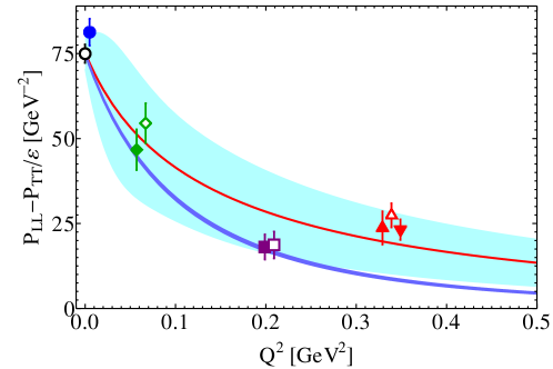
Figure 7: VCS response function $\displaystyle P_{LL}(Q^{2})-P_{TT}(Q^{2})/\varepsilon$. The total $O(p^{3})+O(p^{4}/\varDelta)$ result is given by the red solid curve with the cyan band showing the estimated theoretical uncertainty as explained in the text. DR results Drechsel:2002ar are shown by the blue band. The curves correspond to $\varepsilon=0.65$. The data shown are: black open circle, PDG 2014 Agashe:2014kda ; blue circle, Olmos de León et al Olmos:2001 ; green diamond, MIT-Bates (DR) Bourgeois:2006js ; Bourgeois:2011zz ; green open diamond, MIT-Bates (LEX) Bourgeois:2006js ; Bourgeois:2011zz ; purple solid square, MAMI (DR) Correa:thesis ; purple open square, MAMI (LEX) Correa:thesis ; red solid triangle, MAMI1 (LEX) Roche:2000ng ; red solid inverted triangle, MAMI1 (DR) d'Hose:2006xz ; red open triangle, MAMI2 (LEX) Janssens:2008qe . Some of the data points are shifted to the right in order to enhance their visibility; namely, Olmos de León, MIT-Bates (LEX), MAMI LEX, MAMI1 DR and MAMI2 LEX sets have the same values of $Q^{2}$ as PDG, MIT-Bates (DR), MAMI DR, and MAMI1 LEX, respectively.

The experiments aiming to measure the GPs are based on the low-energy expansion of the $ep\gamma$ process, Eq. (13), which results in the extraction of the VCS response functions. Then, with some further assumptions on the size of spin GPs, taken usually from the fixed-$t$ DR framework of Ref. Drechsel:2002ar , one obtains the two scalar GPs, $\alpha_{E1}$ and $\beta_{M1}$. We first consider our results at the level of the response functions, since it provides a more direct comparison to experiment.

In Figs. 7 to 10, we show our B$\chi$PT results (red solid line, with cyan band indicating the uncertainty estimate), compared with the fixed-$t$ DR calculation (blue bands), and experimental data where available. In this calculation we used the Bradford et al. Bradford:2006yz parametrization of nucleon form factors, as input in Eq. (14). The bands of the DR results are obtained by varying the dipole cut-offs $\Lambda_{\alpha}$ and $\Lambda_{\beta}$ within the uncertainties given in Sec. IV.3.

The first two response functions, $P_{LL}-P_{TT}/\varepsilon$ and $P_{LT}$ (Fig. 7 and 8), are used to extract $\alpha_{E1}(Q^{2})$ and $\beta_{M1}(Q^{2})$, respectively. Our results here are in good agreement with the data as well as with the DR results. The only place of disagreement is $P_{LT}(0)=-2M\beta_{M1}/\alpha_{\mathrm{em}}$, due to the larger value of the static magnetic polarizability resulting in B$\chi$PT, as mentioned already in the previous section.

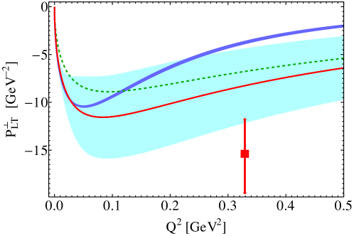
Figure 9: VCS response function $P_{LT}^{\perp}(Q^{2})$. Notation is as in Fig. 7, except from the data: red square, MAMI Doria:2015dyx , and the green dotted curve that shows the B$\chi$PT result with only the contribution of $P_{LL}$ included, see Eq. (15).

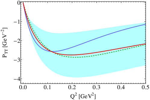
Figure 10: VCS response function $P_{TT}(Q^{2})$. Notation is as in Fig. 7, except from the green dotted curve that shows the B$\chi$PT result with only the contribution of $P^{(M1,M1)1}$ in Eq. (14b).

Apart from these two response functions extracted from unpolarized measurements, there has been a single low-$Q^{2}$ double-polarization experiment at MAMI Doria:2015dyx extracting the response function $P_{LT}^{\perp}$ defined in Eq. (15). This data point, together with theoretical curves, is shown in Fig. 9. This is perhaps the only place where one can see that the B$\chi$PT calculation is in a better agreement with the data than the DR calculation. On the other hand, the slope at $Q^{2}=0$ is in a perfect agreement between the two calculations.

This polarized observable can potentially provide an access to the spin GPs. For instance, combining it with $P_{LL}-P_{TT}/\varepsilon$ one can extract the $P_{TT}$ response function, Fig. 10. The latter is given entirely by the spin GPs. We note that in the $P_{TT}$ response function the large, and well known, $\pi^{0}$ $t$-channel pole contribution to several of the spin GPs drops out. We see from Fig. 10 that the B$\chi$PT and DR results for $P_{TT}$ are again in reasonable agreement.

In Figs. 9 and 10, we also show (by the green dashed curves) the dominant terms in $P_{LT}^{\perp}$ and in $P_{TT}$. They are given by, respectively, $P_{LL}$ and $P^{(M1,M1)1}$ terms in Eqs. (15) and (14b). One thus sees, in particular, that $P^{(L1,M2)1}$, for which the B$\chi$PT and DR results differ sizeably at low $Q^{2}$, gives a very small contribution to $P_{TT}$.

VI Concluding remarks

The B$\chi$PT calculation of the nucleon GPs and VCS response functions, presented here, is done to NLO in the $\delta$-counting scheme. It shows a good description of the low-$Q$ data and mostly agrees with the results of the fixed-$t$ DR calculation of Pasquini et al. Pasquini:2001yy . The results for the scalar GPs are summarized in Fig. 11, where panel (a) shows the electric polarizability and panel (b)—the magnetic one. The theoretical uncertainty of our calculation is sufficiently large to agree with all the data, including the new Correa:thesis and old Roche:2000ng ; Janssens:2008qe MAMI data that tend to disagree among themselves. We can see that the DR curve agrees with the new MAMI data very well, while missing the older data, especially for $\alpha_{E1}$. For $\beta_{M1}$, there is an interesting tension at low $Q$ between the DR and $\chi$PT results. The available VCS data do not have the necessary precision to resolve the discrepancy.

By making the heavy-baryon expansion we reproduce some of the previous HB$\chi$PT results and, similarly to what was observed in the calculation of the real CS, we find that treating the leading chiral loops exactly allows for a more natural accommodation of the Delta-resonance contribution, which is especially large in the magnetic polarizability $\beta_{M1}$.

Figure 11: Generalized scalar polarizabilities: (a) $\alpha_{E1}(Q^{2})$, (b) $\beta_{M1}(Q^{2})$. Description of curves and points is the same as in Fig. 7.

We would like to note that a newly approved experiment at Jefferson Lab JLab_C12-15-001 which plans to measure the unpolarized GPs at $Q^{2}=0.3$ GeV² and $Q^{2}=0.75$ GeV² will be able to shed further light on the situation. Furthermore, comparing such data at the same $Q^{2}$ value taken at different values of $\varepsilon$ (corresponding with different beam energies) has the potential to separate off the response function $P_{TT}$ in Eq. (13). This would allow one to experimentally access the dominant spin GP $P^{(M1,M1)1}$ for the first time and provide a strong test of the B$\chi$PT predictions presented in this work.

Additionally, new data on the unpolarized response functions and GPs are expected to arrive soon from MAMI. These data will complement the $Q^{2}=0.2$ GeV² points Correa:thesis . In particular, expected are data at $Q^{2}=0.1$ GeV² and $Q^{2}=0.45$ GeV², which is in the domain of applicability of B$\chi$PT. These data will also further test the theoretical predictions.

One has to admit that the current theoretical uncertainty estimate gives a rather sizeable error band, which should be improved upon. An $O(p^{4})$ calculation of GPs in B$\chi$PT that would include the remaining $\pi\Delta$ loops that contribute at $O(p^{3})$ in the high-momenta regime and both the $\pi N$ and the $\pi\Delta$ $O(p^{4})$ contributions in this regime would allow one to significantly decrease the theoretical uncertainty.

Appendix A Tensor decomposition of the VCS amplitude

In this section we give the details of the tensor decomposition of the VCS amplitude. The basis used by us is $\rho_{i}$, $i=1,\dots,12$, introduced in Ref. Drechsel:1997xv . Its decomposition in terms of Tarrach’s $T_{1},\dots,T_{34}$ (which are given below) reads

$$\rho_{1}= -q\cdot q^{\prime}T_{1}+T_{3}\,,$$

$$\rho_{2}= -4M^{2}\xi^{2}T_{1}-4q\cdot q^{\prime}T_{6}+4M\xi T_{7}\,,$$

$$\rho_{3}= -2M\xi Q^{2}T_{1}-M\xi(T_{4}+T_{5})+Q^{2}(T_{7}-T_{8})+q\cdot q^{\prime}(T_{9}-T_{10})\,,$$

$$\rho_{4}= 8T_{16}-4M\xi T_{21}+M\xi T_{34}\,,$$

$$\rho_{5}= \frac{1}{2}(T_{19}-T_{20})-\frac{Q^{2}}{2}T_{22}-\frac{M\xi}{2}(T_{23}+T_{24})-\frac{Q^{2}}{8}T_{34}\,,$$

$$\rho_{6}= -8q\cdot q^{\prime}T_{6}+4M\xi T_{7}+4Mq\cdot q^{\prime}T_{21}-4M^{2}\xi T_{25}-2M\xi(T_{32}+q\cdot q^{\prime}T_{33})+Mq\cdot q^{\prime}T_{34}\,,$$

$$\rho_{7}= T_{18}-q\cdot q^{\prime}T_{22}+M\xi T_{26}\,,$$

$$\rho_{8}= \frac{M\xi}{2}(T_{4}+T_{5})+\frac{Q^{2}}{2}T_{8}-\frac{q\cdot q^{\prime}}{2}(T_{9}-T_{10})-\frac{M}{2}(T_{14}+T_{15})+\frac{Mq\cdot q^{\prime}}{2}(T_{23}+T_{24})+\frac{MQ^{2}}{2}T_{26}$$

$$+\frac{Q^{2}}{4}(T_{32}+q\cdot q^{\prime}T_{33})\,,$$

$$\rho_{9}= 2M\xi T_{8}-2Mq\cdot q^{\prime}T_{22}+2M^{2}\xi T_{26}-q\cdot q^{\prime}T_{27}+M\xi T_{31}\,,$$

$$\rho_{10}= 2T_{7}+4MT_{11}-2MT_{25}-4M\xi T_{1}+(T_{32}+q\cdot q^{\prime}T_{33})\,,$$

$$\rho_{11}= 4T_{17}-4M\xi T_{25}+q\cdot q^{\prime}T_{34}\,,$$

$$\rho_{12}= 2Q^{2}T_{6}+M\xi(T_{9}-T_{10})-MQ^{2}(T_{21}+T_{22})-M^{2}\xi(T_{23}+T_{24})-\frac{Q^{2}}{2}(T_{27}-M\xi T_{33})$$

$$-\frac{M\xi}{2}(T_{29}+T_{30})-\frac{MQ^{2}}{4}T_{34}\,.$$ (31)

These tensors correspond to the following combinations of Tarrach’s $\tau_{i}$ (with $q^{\prime 2}$ set to zero in the latter):

$$\rho_{1} =-\tau_{1}, \rho_{2} =-4\tau_{3}, \rho_{3} =\tau_{4}-\tau_{5}, \rho_{4} =\tau_{7},$$

$$\rho_{5} =\frac{1}{2}(\tau_{8}-\tau_{9}), \rho_{6} =\tau_{10}, \rho_{7} =\tau_{11}, \rho_{8} =\frac{1}{2}(\tau_{12}+\tau_{13}),$$ (32)

$$\rho_{9} =\tau_{14}, \rho_{10} =\tau_{17}, \rho_{11} =\tau_{18}, \rho_{12} =\frac{1}{2}(\tau_{20}+\tau_{21})\,.$$

All tensors apart from $\rho_{2}$, $\rho_{3}$, and $\rho_{6}$ have unique structures that allow for unambiguous identification, e.g., the combination $T_{29}+T_{30}$ enters only $\rho_{12}$, $T_{17}$ enters only $\rho_{11}$, and so on. After the tensors $\rho_{i}$, $i\neq 2,3,6$, have been identified, the remaining tensors can be identified as well. Since this basis is explicitly gauge invariant, all the terms that are not proportional to any of $\rho_{i}$ have to vanish when one decomposes a gauge invariant amplitude, e.g., summing up a gauge invariant subset of Feynman graphs.

The tensors $T_{1},\dots,T_{34}$ introduced by Tarrach Tarrach:1975tu in order to decompose the CS amplitude in the most general case, i.e., when both $q^{2}$ and $q^{\prime 2}$ are non-zero, are given below; these structures are understood to be contracted with $\epsilon^{\nu}$ and $\epsilon^{*\mu}$, the incoming and the outgoing photons’ polarization vectors.

$$T_{1}=g_{\mu\nu}\,, \qquad T_{17}=\left(P_{\nu}q_{\mu}+P_{\mu}q^{\prime}_{\nu}\right)\not{K}\,,$$

$$T_{2}=q_{\nu}q^{\prime}_{\mu}\,, \qquad T_{18}=\left(P_{\nu}q_{\mu}-P_{\mu}q^{\prime}_{\nu}\right)\not{K}\,,$$

$$T_{3}=q^{\prime}_{\nu}q_{\mu}\,, \qquad T_{19}=\left(P_{\nu}q^{\prime}_{\mu}+P_{\mu}q_{\nu}\right)\not{K}\,,$$

$$T_{4}=q_{\nu}q_{\mu}+q^{\prime}_{\nu}q^{\prime}_{\mu}\,, \qquad T_{20}=\left(P_{\nu}q^{\prime}_{\mu}-P_{\mu}q_{\nu}\right)\not{K}\,,$$

$$T_{5}=q_{\nu}q_{\mu}-q^{\prime}_{\nu}q^{\prime}_{\mu}\,, \qquad T_{21}=P_{\nu}\gamma_{\mu}+P_{\mu}\gamma_{\nu}\,,$$

$$T_{6}=P_{\nu}P_{\mu}\,, \qquad T_{22}=P_{\nu}\gamma_{\mu}-P_{\mu}\gamma_{\nu}\,,$$

$$T_{7}=P_{\nu}q_{\mu}+P_{\mu}q^{\prime}_{\nu}\,, \qquad T_{23}=q_{\nu}\gamma_{\mu}+q^{\prime}_{\mu}\gamma_{\nu}\,,$$

$$T_{8}=P_{\nu}q_{\mu}-P_{\mu}q^{\prime}_{\nu}\,, \qquad T_{24}=q_{\nu}\gamma_{\mu}-q^{\prime}_{\mu}\gamma_{\nu}\,,$$

$$T_{9}=P_{\nu}q^{\prime}_{\mu}+P_{\mu}q_{\nu}\,, \qquad T_{25}=q^{\prime}_{\nu}\gamma_{\mu}+q_{\mu}\gamma_{\nu}\,,$$

$$T_{10}=P_{\nu}q^{\prime}_{\mu}-P_{\mu}q_{\nu}\,, \qquad T_{26}=q^{\prime}_{\nu}\gamma_{\mu}-q_{\mu}\gamma_{\nu}\,,$$ (33)

$$T_{11}=g_{\mu\nu}\not{K}\,, \qquad T_{27}=2\left(P_{\nu}\gamma_{\mu\lambda}K^{\lambda}+P_{\mu}\gamma_{\nu\lambda}K^{\lambda}\right)\,,$$

$$T_{12}=q_{\nu}q^{\prime}_{\mu}\not{K}\,, \qquad T_{28}=2\left(P_{\nu}\gamma_{\mu\lambda}K^{\lambda}-P_{\mu}\gamma_{\nu\lambda}K^{\lambda}\right)\,,$$

$$T_{13}=q^{\prime}_{\nu}q_{\mu}\not{K}\,, \qquad T_{29}=2\left(q_{\nu}\gamma_{\mu\lambda}K^{\lambda}+q^{\prime}_{\mu}\gamma_{\nu\lambda}K^{\lambda}\right)\,,$$

$$T_{14}=(q_{\nu}q_{\mu}+q^{\prime}_{\nu}q^{\prime}_{\mu})\not{K}\,, \qquad T_{30}=2\left(q_{\nu}\gamma_{\mu\lambda}K^{\lambda}-q^{\prime}_{\mu}\gamma_{\nu\lambda}K^{\lambda}\right)\,,$$

$$T_{15}=(q_{\nu}q_{\mu}-q^{\prime}_{\nu}q^{\prime}_{\mu})\not{K}\,, \qquad T_{31}=2\left(q^{\prime}_{\nu}\gamma_{\mu\lambda}K^{\lambda}+q_{\mu}\gamma_{\nu\lambda}K^{\lambda}\right)\,,$$

$$T_{16}=P_{\nu}P_{\mu}\not{K}\,, \qquad T_{32}=2\left(q^{\prime}_{\nu}\gamma_{\mu\lambda}K^{\lambda}-q_{\mu}\gamma_{\nu\lambda}K^{\lambda}\right)\,,$$

$$\qquad T_{33}=2\gamma_{\nu\mu}\,,$$

$$\qquad T_{34}=2\left\{\gamma_{\nu\mu},\not{K}\right\}=4\gamma_{\nu\mu\lambda}K^{\lambda}\,.$$

Here, $P=\mbox{\small{$\frac{1}{2}$}}(p+p^{\prime})$, $K=\mbox{\small{$\frac{1}{2}$}}(q+q^{\prime})$, $\gamma^{\mu\nu}=\mbox{\small{$\frac{1}{2}$}}[\gamma^{\mu},\gamma^{\nu}]$ and $\gamma^{\mu\nu\lambda}=\mbox{\small{$\frac{1}{2}$}}\{\gamma^{\mu\nu},\gamma^{\lambda}\}$. The following relations hold between these tensors that allow one to exclude two of them (the usual choice being $T_{13}$ and $T_{28}$):

$$\begin{split}2(T_{17}-T_{19})-(q^{2}-q^{\prime 2})T_{22}+2P\cdot K(T_{23}-T_{25})&-2MT_{28}-2MP\cdot K\,T_{32}\\ &+\left(M^{2}+\frac{q.q^{\prime}}{4}-\frac{q^{2}+q^{\prime 2}}{4}\right)T_{34}=0\,,\end{split}$$ (34)

$$\begin{split}&P\cdot K(T_{2}-T_{3})+\frac{1}{4}(q^{2}+q^{\prime 2}+2q\cdot q^{\prime})(T_{7}-T_{9})-\frac{q^{2}-q^{\prime 2}}{4}(T_{8}+T_{10})-M(T_{12}-T_{13})\\ &+\frac{M}{4}(q^{2}+q^{\prime 2}+2q\cdot q^{\prime})(T_{23}-T_{25})-M\frac{q^{2}-q^{\prime 2}}{4}(T_{24}+T_{26})-P\cdot K\,T_{28}+\frac{q^{2}-q^{\prime 2}}{8}(T_{29}-T_{31})\\ &-\frac{1}{8}(q^{2}+q^{\prime 2}-2q\cdot q^{\prime})(T_{30}+T_{32})-\left[\left(P\cdot K\right)^{2}+\frac{1}{4}\left(q^{2}q^{\prime 2}-(q\cdot q^{\prime})^{2}\right)\right]T_{33}+\frac{M}{2}P\cdot K\,T_{34}=0\,.\end{split}$$ (35)

Taking into account the fact that for the (real) final photon $\epsilon^{\prime}\cdot q^{\prime}=0$, one can obtain the following useful identities:

$$T_{2}=0,\quad T_{4}=T_{5},\quad T_{9}=-T_{10},\quad T_{12}=0,\quad T_{14}=T_{15},\quad T_{19}=-T_{20},\quad T_{23}=T_{24},\quad T_{29}=T_{30}\,.$$ (36)

Appendix B Invariant amplitudes

Here we provide expressions for the linear combinations of invariant amplitudes $\bar{A}_{i}(Q^{2})=\bar{A}_{i}(0,-Q^{2},-Q^{2})$ that contribute to the generalized polarizabilities, see Eqs. (9a)-(9f):

$$g_{1}=\bar{A}_{1},\ g_{2}=\bar{A}_{2},\ g_{3}=\bar{A}_{5},\ g_{4}=\bar{A}_{5}+\bar{A}_{7}+4\bar{A}_{11},\ g_{5}=2\bar{A}_{6}+\bar{A}_{9},\ g_{6}=\bar{A}_{12}\,.$$ (37)

The results are given for the $\pi$N loop and Delta pole contributions; for the $\pi\Delta$ loop results, see supplementary material to this article.

B.1 $\pi N$ loops

Here, $D_{1}(x,y)=\left[\tau(1-x)^{2}(1-4y^{2})+D_{N}(x)\right]^{-1}$, $D_{2}(x,y)=\left[\tau x^{2}(1-4y^{2})+D_{N}(x)\right]^{-1}$, $D_{0}(x,y)=\left[D_{N}(x)\right]^{-1}$, and $D_{\pi}(x,y)=\left[4\tau(1-x)x+\mu^{2}\right]^{-1}$. In turn, $D_{N}(x)=x^{2}+\mu^{2}(1-x)$. The amplitudes are expressed as integrals over the Feynman parameters as follows:

$$g_{i}(Q^{2})=\frac{g_{A}^{2}}{8\pi^{2}f_{\pi}^{2}M^{n_{i}}}\int\limits_{0}^{1}\mathrm{d}x\int\limits_{-1/2}^{1/2}\mathrm{d}y\,\phi_{i}(\tau,x,y)\,,$$ (38)

where $\phi_{i}$ are given below, $g_{A}=1.27$ and $f_{\pi}=92.21$ MeV are the axial coupling constant and the pion decay constant, and $n_{i}=1,3,2,2,3,3$ for $i=1,2,3,4,5,6$ account for the correct dimensions of the respective $g_{i}$.

B.1.1 Proton

$$\phi_{1}= -\frac{1}{2}D_{1}^{2}(x,y)(x-1)^{3}x\left(-4y^{2}+2x+1\right)-\frac{1}{4}D_{2}^{2}(x,y)x^{4}\left(4y^{2}+2x-1\right)$$

$$-\frac{1}{2}D_{0}^{2}(x,y)x^{3}\left(3x^{2}-5x+2\right)-2D_{\pi}(x,y)(x-1)^{2}x\,,$$ (39)

$$\phi_{2}= 4D_{1}^{4}(x,y)y^{2}\left(4y^{2}-1\right)\tau(x-1)^{6}x^{3}$$

$$-\frac{1}{3}D_{1}^{3}(x,y)(x-1)^{4}x\left(4y^{2}\left(4y^{2}-1\right)\tau+x^{2}\left(8y^{2}\tau-1\right)-4y^{2}\left(4y^{2}+1\right)\tau x\right)$$

$$+\frac{1}{24}D_{1}^{2}(x,y)(x-1)^{3}x\left(\left(36y^{2}-7\right)x+4\right)$$

$$+2D_{2}^{4}(x,y)y^{2}\left(4y^{2}-1\right)\tau(x-1)^{2}x^{7}$$

$$-\frac{1}{12}D_{2}^{3}(x,y)(x-1)x^{5}\left(\tau\left(-48y^{4}+2\left(36y^{4}-5y^{2}+1\right)x-1\right)+2\left(3y^{2}(x-2)-1\right)\right)$$

$$+\frac{1}{16}D_{2}^{2}(x,y)x^{3}\left(-4y^{2}+\left(4y^{2}+5\right)x^{2}-8x+3\right)$$

$$-\frac{3}{2}D_{0}^{4}(x,y)(x-1)^{2}x^{4}\left(\mu^{2}+\left(\mu^{2}-1\right)x^{2}-2\mu^{2}x\right)$$

$$+\frac{1}{12}D_{0}^{3}(x,y)(x-1)x^{2}\left(-18\mu^{2}+10x^{4}+9\left(\mu^{2}-3\right)x^{3}+\left(26-36\mu^{2}\right)x^{2}+45\mu^{2}x\right)$$

$$-\frac{1}{6}D_{0}^{2}(x,y)(x-2)(x-1)^{2}\,,$$ (40)

$$\phi_{3}= \frac{1}{2}D_{1}^{2}(x,y)(x-1)^{2}x\left(8y^{2}+\left(8y^{2}+1\right)x^{2}-16y^{2}x\right)+\frac{1}{4}D_{2}^{2}(x,y)x^{4}\left(8y^{2}x+x-1\right)$$

$$+\frac{1}{4}D_{0}^{2}(x,y)x^{3}\left(3x^{2}-5x+2\right)\,,$$ (41)

$$\phi_{4}= \frac{1}{2}D_{1}^{2}(x,y)(x-1)^{3}x\left(4y^{2}(4x-3)+1\right)+\frac{1}{4}D_{2}^{2}(x,y)x^{4}\left(4y^{2}(4x-3)-1\right)\,,$$ (42)

$$\phi_{5}= -2D_{1}^{3}(x,y)y^{2}\left(4y^{2}-1\right)\tau(x-1)^{5}x^{2}-\frac{1}{4}D_{1}^{2}(x,y)(x-1)^{3}x\left(-4y^{2}+\left(12y^{2}-1\right)x+1\right)$$

$$+\frac{1}{12}D_{2}^{3}(x,y)(x-1)x^{5}\left(-12y^{2}+\left(4y^{2}-1\right)\tau\left(-8y^{2}+2\left(6y^{2}-1\right)x+1\right)+2x-1\right)$$

$$-\frac{1}{48}D_{2}^{2}(x,y)x^{3}\left(-12y^{2}+16x^{2}+\left(12y^{2}-25\right)x+9\right)$$

$$+\frac{3}{2}D_{0}^{4}(x,y)(x-1)^{2}x^{4}\left(\mu^{2}+\left(\mu^{2}-1\right)x^{2}-2\mu^{2}x\right)$$

$$-\frac{1}{12}D_{0}^{3}(x,y)(x-1)x^{2}\left(-18\mu^{2}+10x^{4}+9\left(\mu^{2}-3\right)x^{3}+\left(26-36\mu^{2}\right)x^{2}+45\mu^{2}x\right)$$

$$+\frac{1}{12}D_{0}^{2}(x,y)(x-1)^{2}x^{2}(5x-6)\,,$$ (43)

$$\phi_{6}= -4D_{1}^{3}(x,y)y^{2}(x-1)^{4}x^{3}-2D_{2}^{3}(x,y)y^{2}(x-1)x^{6}\,.$$ (44)

B.1.2 Neutron

$$\phi_{1}= \frac{1}{2}D_{1}^{2}(x,y)(x-1)^{2}x\left(-4y^{2}+4y^{2}x+x+1\right)-\frac{1}{2}D_{2}^{2}(x,y)\left(4y^{2}+1\right)x^{4}$$

$$-2D_{\pi}(x,y)(x-1)^{2}x\,,$$ (45)

$$\phi_{2}= -4D_{1}^{4}(x,y)y^{2}\left(4y^{2}-1\right)\tau(x-1)^{5}x^{3}$$

$$+\frac{1}{12}D_{1}^{3}(x,y)(x-1)^{2}x$$

$$\hskip 28.45274pt\times\left(4y^{2}\tau\left(x^{2}+x-2\right)^{2}-x^{2}\left(\tau(x-1)^{2}+x(x+2)-4\right)+64y^{4}\tau(x-1)^{3}\right)$$

$$+\frac{1}{24}D_{1}^{2}(x,y)(x-1)^{2}x(x(4x-1)-4)$$

$$+4D_{2}^{4}(x,y)y^{2}\left(4y^{2}-1\right)\tau(x-1)^{2}x^{6}$$

$$-\frac{1}{12}D_{2}^{3}(x,y)(x-1)x^{4}$$

$$\hskip 28.45274pt\times\left(4y^{2}\left(\tau\left(2x^{2}+x-8\right)+3(x-2)x\right)-48y^{4}\tau(x-2)x+x\left(\tau(x+1)+x-3\right)-2\right)$$

$$+\frac{1}{24}D_{2}^{2}(x,y)(x-1)x^{2}\left(4x^{2}+24y^{2}(2x-1)x+x+1\right)\,,$$ (46)

$$\phi_{3}= -\frac{1}{2}D_{1}^{2}(x,y)(x-1)x\left(8y^{2}+\left(8y^{2}+1\right)x^{2}-16y^{2}x\right)+\frac{1}{2}D_{2}^{2}(x,y)x^{3}\left(8y^{2}x+x-1\right)\,,$$ (47)

$$\phi_{4}= \frac{1}{2}D_{1}^{2}(x,y)(x-1)^{3}x\left(4y^{2}(4x-3)+1\right)+\frac{1}{4}D_{2}^{2}(x,y)x^{4}\left(4y^{2}(4x-3)-1\right)\,,$$ (48)

$$\phi_{5}= -\frac{1}{6}D_{1}^{3}(x,y)(x-1)^{2}x^{3}\left(\left(4y^{2}-1\right)\tau(x-1)^{2}-(x-2)x\right)$$

$$-\frac{1}{12}D_{1}^{2}(x,y)(x-1)^{2}x\left(12y^{2}+4x^{2}-3\left(4y^{2}+1\right)x-3\right)$$

$$-\frac{1}{12}D_{2}^{3}(x,y)(x-1)x^{5}\left(\left(4y^{2}-1\right)\tau\left(-20y^{2}+12y^{2}x+x+1\right)+36y^{2}-12y^{2}x-x-1\right)$$

$$-\frac{1}{24}D_{2}^{2}(x,y)(x-1)x^{3}\left(-36y^{2}+\left(48y^{2}+4\right)x+3\right)\,,$$ (49)

$$\phi_{6}= 4D_{1}^{3}(x,y)y^{2}(x-1)^{3}x^{3}-4D_{2}^{3}(x,y)y^{2}(x-1)x^{5}\,.$$ (50)

B.2 Delta pole

Here, $g_{E}$ and $g_{M}$ are the electric and magnetic $\gamma N\Delta$ couplings Pascalutsa:2002pi , $M_{+}=M_{\Delta}+M$, and

$$f_{M}=\frac{g_{M}}{\big{[}1+\left(Q/\Lambda\right)^{2}\big{]}^{2}}$$

is the magnetic $\gamma N\Delta$ coupling modified by the dipole form factor, with $\Lambda^{2}=0.71$ GeV².

$$g_{1} =\frac{f_{M}\left[2g_{M}\,M_{+}\left(4M^{2}+Q^{2}\right)-g_{E}\,Q^{2}\varDelta\right]+g_{E}\,Q^{2}(g_{M}\,M_{+}-2g_{E}\,\varDelta)}{4M^{2}M_{+}^{3}\varDelta}\,,$$ (51)

$$g_{2} =-\frac{f_{M}\,g_{M}\,M_{+}-g_{E}^{2}\,\varDelta}{2M^{2}M_{+}^{3}\varDelta}\,,$$ (52)

$$g_{3} =\frac{f_{M}\left(8M^{2}+Q^{2}\right)(g_{M}M_{+}-2g_{E}\,\varDelta)+g_{E}\left[2g_{M}\,M_{+}Q^{2}-g_{E}\,\varDelta\left(8M^{2}+Q^{2}\right)\right]}{8M^{3}M_{+}^{3}\varDelta}\,,$$ (53)

$$g_{4} =\frac{f_{M}\,g_{M}\,M_{+}-2f_{M}\,g_{E}\,\varDelta-2g_{E}^{2}\,\varDelta+3g_{E}\,g_{M}\,M_{+}}{MM_{+}^{3}\varDelta}\,,$$ (54)

$$g_{5} =-\frac{f_{M}\,g_{M}\,M_{+}-3f_{M}\,g_{E}\,\varDelta-g_{E}^{2}\,\varDelta+3g_{E}\,g_{M}\,M_{+}}{4M^{2}M_{+}^{3}\varDelta}\,,$$ (55)

$$g_{6} =-\frac{f_{M}\,g_{M}\,M_{+}-2f_{M}\,g_{E}\,\varDelta-g_{E}^{2}\,\varDelta+2g_{E}\,g_{M}\,M_{+}}{4M^{2}M_{+}^{3}\varDelta}\,.$$ (56)

References

- (1) R. A. Berg and C. N. Lindner, Phys. Rev. 112 (1958) 2072.
- (2) R. A. Berg and C. N. Lindner, Nucl. Phys. 26 (1961) 259.
- (3) P. A. M. Guichon, G. Q. Liu and A. W. Thomas, Nucl. Phys. A 591 (1995) 606 [nucl-th/9605031].
- (4) P. A. M. Guichon and M. Vanderhaeghen, Prog. Part. Nucl. Phys. 41 (1998) 125 [hep-ph/9806305].
- (5) M. Gorchtein, C. Lorcé, B. Pasquini and M. Vanderhaeghen, Phys. Rev. Lett. 104 (2010) 112001.
- (6) D. Drechsel, G. Knöchlein, A. Y. Korchin, A. Metz and S. Scherer, Phys. Rev. C 57 (1998) 941.
- (7) D. Drechsel, G. Knöchlein, A. Y. Korchin, A. Metz and S. Scherer, Phys. Rev. C 58 (1998) 1751.
- (8) P. Bourgeois et al., Phys. Rev. Lett. 97 (2006) 212001 [nucl-ex/0605009].
- (9) P. Bourgeois et al., Phys. Rev. C 84 (2011) 035206.
- (10) J. Roche et al. [VCS and A1 Collaborations], Phys. Rev. Lett. 85 (2000) 708 [hep-ex/0007053].
- (11) P. Janssens et al. [A1 Collaboration], Eur. Phys. J. A 37 (2008) 1 [arXiv:0803.0911 [nucl-ex]].
- (12) N. d’Hose, Eur. Phys. J. A 28S1 (2006) 117.
- (13) L. Doria et al. [A1 Collaboration], Phys. Rev. C 92 (2015) 054307 [arXiv:1505.06106 [nucl-ex]].
- (14) L. Correa, Measurement of the generalized polarizabilities of the proton by virtual Compton scattering at MAMI and GeV2, PhD Thesis, Mainz–Clermont-Ferrand (2016).
- (15) T. R. Hemmert, B. R. Holstein, G. Knöchlein and S. Scherer, Phys. Rev. Lett. 79 (1997) 22 [nucl-th/9705025].
- (16) T. R. Hemmert, B. R. Holstein, G. Knöchlein and S. Scherer, Phys. Rev. D 55 (1997) 2630 [nucl-th/9608042].
- (17) T. R. Hemmert, B. R. Holstein, G. Knöchlein and D. Drechsel, Phys. Rev. D 62 (2000) 014013.
- (18) C. W. Kao and M. Vanderhaeghen, Phys. Rev. Lett. 89 (2002) 272002 [hep-ph/0209336].
- (19) C. W. Kao, B. Pasquini and M. Vanderhaeghen, Phys. Rev. D 70 (2004) 114004 [Erratum: Phys. Rev. D 92 (2015) 119906] [hep-ph/0408095].
- (20) B. Pasquini, M. Gorchtein, D. Drechsel, A. Metz and M. Vanderhaeghen, Eur. Phys. J. A 11 (2001) 185 [hep-ph/0102335].
- (21) D. Drechsel, B. Pasquini and M. Vanderhaeghen, Phys. Rept. 378 (2003) 99 [hep-ph/0212124].
- (22) T. Becher and H. Leutwyler, Eur. Phys. J. C 9 (1999) 643 [hep-ph/9901384].
- (23) T. Fuchs, J. Gegelia, G. Japaridze and S. Scherer, Phys. Rev. D 68 (2003) 056005 [hep-ph/0302117].
- (24) V. Pascalutsa, B. R. Holstein and M. Vanderhaeghen, Phys. Lett. B 600 (2004) 239 [hep-ph/0407313].
- (25) B. R. Holstein, V. Pascalutsa and M. Vanderhaeghen, Phys. Rev. D 72 (2005) 094014 [hep-ph/0507016].
- (26) V. Pascalutsa and M. Vanderhaeghen, Phys. Rev. D 73 (2006) 034003 [hep-ph/0512244].
- (27) T. Ledwig, J. Martin-Camalich, V. Pascalutsa and M. Vanderhaeghen, Phys. Rev. D 85 (2012) 034013 [arXiv:1108.2523 [hep-ph]].
- (28) J. M. Alarcón, J. Martin-Camalich and J. A. Oller, Phys. Rev. D 85 (2012) 051503 [arXiv:1110.3797 [hep-ph]].
- (29) J. M. Alarcón, J. Martin-Camalich and J. A. Oller, Annals Phys. 336 (2013) 413 [arXiv:1210.4450 [hep-ph]].
- (30) A. N. Hiller Blin, T. Ledwig and M. J. Vicente Vacas, Phys. Rev. D 93 (2016) 094018 [arXiv:1602.08967 [hep-ph]].
- (31) D. L. Yao, D. Siemens, V. Bernard, E. Epelbaum, A. M. Gasparyan, J. Gegelia, H. Krebs and U.-G. Meißner, JHEP 1605 (2016) 038 [arXiv:1603.03638 [hep-ph]].
- (32) V. Pascalutsa, Prog. Part. Nucl. Phys. 55 (2005) 23 [nucl-th/0412008].
- (33) J. M. M. Hall and V. Pascalutsa, Eur. Phys. J. C 72 (2012) 2206 [arXiv:1203.0724 [hep-ph]].
- (34) V. Bernard, E. Epelbaum, H. Krebs and U. G. Meißner, Phys. Rev. D 87 (2013) 054032 [arXiv:1209.2523 [hep-ph]].
- (35) V. Lensky and V. Pascalutsa, Eur. Phys. J. C 65 (2010) 195 [arXiv:0907.0451 [hep-ph]].
- (36) V. Lensky, J. M. Alarcón and V. Pascalutsa, Phys. Rev. C 90 (2014) 055202 [arXiv:1407.2574 [hep-ph]].
- (37) V. Lensky, J. A. McGovern and V. Pascalutsa, Eur. Phys. J. C 75 (2015) 604 [arXiv:1510.02794 [hep-ph]].
- (38) G. Eichmann and C. S. Fischer, Phys. Rev. D 87 (2013) 036006 [arXiv:1212.1761 [hep-ph]].
- (39) F. E. Low, Phys. Rev. 96 (1954) 1428.
- (40) S. Scherer, A. Y. Korchin and J. H. Koch, Phys. Rev. C 54 (1996) 904 [nucl-th/9605030].
- (41) V. Pascalutsa and M. Vanderhaeghen, Phys. Rev. D 91 (2015) 051503 [arXiv:1409.5236 [nucl-th]].
- (42) V. Lensky, V. Pascalutsa, M. Vanderhaeghen and C. W. Kao, arXiv:1701.01947 [hep-ph].
- (43) F. Hagelstein, R. Miskimen and V. Pascalutsa, Prog. Part. Nucl. Phys. 88 (2016) 29 [arXiv:1512.03765 [nucl-th]].
- (44) M. Vanderhaeghen, Phys. Lett. B 402 (1997) 243.
- (45) S. Weinberg, Physica A 96 (1979) 327.
- (46) J. Gasser and H. Leutwyler, Annals Phys. 158 (1984) 142.
- (47) J. Gasser, M. E. Sainio and A. Švarc, Nucl. Phys. B 307 (1988) 779.
- (48) V. Pascalutsa, M. Vanderhaeghen and S. N. Yang, Phys. Rept. 437 (2007) 125
- (49) L. Geng, Front. Phys. (Beijing) 8 (2013) 328 [arXiv:1301.6815 [nucl-th]].
- (50) V. Pascalutsa and D. R. Phillips, Phys. Rev. C 67, 055202 (2003) [nucl-th/0212024].
- (51) R. Tarrach, Nuovo Cim. A 28 (1975) 409.
- (52) V. Lensky and J. A. McGovern, Phys. Rev. C 89 (2014) 032202 [arXiv:1401.3320 [nucl-th]].
- (53) A. Metz and D. Drechsel, Z. Phys. A 356 (1996) 351.
- (54) A. Metz and D. Drechsel, Z. Phys. A 359 (1997) 165 [nucl-th/9705010].
- (55) T. R. Hemmert, B. R. Holstein and J. Kambor, Phys. Lett. B 395 (1997) 89 [hep-ph/9606456].
- (56) D. Drechsel, S. S. Kamalov and L. Tiator, Eur. Phys. J. A 34, 69 (2007). arXiv:0710.0306 [nucl-th].
- (57) H. W. Grießhammer, J. A. McGovern, D. R. Phillips and G. Feldman, Prog. Part. Nucl. Phys. 67 (2012) 841 [arXiv:1203.6834 [nucl-th]].
- (58) B. Pasquini, D. Drechsel and M. Vanderhaeghen, Phys. Rev. C 76, 015203 (2007) arXiv:0705.0282 [hep-ph].
- (59) J. A. McGovern, D. R. Phillips and H. W. Grießhammer, Eur. Phys. J. A 49, 12 (2013) arXiv:1210.4104 [nucl-th].
- (60) H. W. Grießhammer, J. A. McGovern and D. R. Phillips, Eur. Phys. J. A 52 (2016) 139 [arXiv:1511.01952 [nucl-th]].
- (61) P. P. Martel et al. [A2 Collaboration], Phys. Rev. Lett. 114, 112501 (2015) arXiv:1408.1576 [nucl-ex].
- (62) K. A. Olive et al. [Particle Data Group Collaboration], Chin. Phys. C 38, 090001 (2014).
- (63) V. Olmos de León et al., Eur. Phys. J. A 10, 207 (2001).
- (64) R. Bradford, A. Bodek, H. S. Budd and J. Arrington, Nucl. Phys. Proc. Suppl. 159 (2006) 127 [hep-ex/0602017].
- (65) Jefferson Lab Experiment C12-15-001, Co-spokespersons M. Paolone, N. Sparveris (contact person), A. Camsonne, and M. Jones, PAC44, https://www.jlab.org/exp_prog/proposals/16/C12-15-001.pdf.
- (66) J. A. M. Vermaseren, math-ph/0010025.
- (67) D. Binosi, J. Collins, C. Kaufhold and L. Theussl, Comput. Phys. Commun. 180 (2009) 1709 [arXiv:0811.4113 [hep-ph]].