Abstract

We explore a two component dark matter model with a fermion and a scalar. In this scenario the Standard Model (SM) is extended by a fermion, a scalar and an additional pseudo scalar. The fermionic component is assumed to have a global ${\rm U(1)}_{\rm DM}$ and interacts with the pseudo scalar via Yukawa interaction while a $\mathbb{Z}_{2}$ symmetry is imposed on the other component – the scalar. These ensure the stability of both the dark matter components. Although the Lagrangian of the present model is CP conserving, however the CP symmetry breaks spontaneously when the pseudo scalar acquires a vacuum expectation value (VEV). The scalar component of the dark matter in the present model also develops a VEV on spontaneous breaking of the $\mathbb{Z}_{2}$ symmetry. Thus the various interactions of the dark sector and the SM sector are progressed through the mixing of the SM like Higgs boson, the pseudo scalar Higgs like boson and the singlet scalar boson. We show that the observed gamma ray excess from the Galactic Centre, self-interaction of dark matter from colliding clusters as well as the 3.55 keV X-ray line from Perseus, Andromeda etc. can be simultaneously explained in the present two component dark matter model.

1 Introduction

The observational results from the satellite borne experiment WMAP [1] and more recently Planck [2] have now firmly established the presence of dark matter (DM) in the Universe. Their results reveal that more than 80% matter content of the Universe are in the form of mysterious unknown matter called the dark matter. Until now, only the gravitational interactions of DM have been manifested by most of its indirect evidences namely the flatness of rotation curves of spiral galaxies [3], gravitational lensing [4], phenomena of Bullet cluster [5] and other various colliding galaxy clusters etc. However, the particle nature of DM still remains an enigma. There are various ongoing dark matter direct detection experiments such as LUX [6], XENON-1T [7], PandaX-II [8] etc. which have been trying to investigate the particle nature as well as the interaction type (spin dependent or spin independent) of DM with the visible sector by measuring the recoil energy of the scattered detector nuclei. However, the null results of these experiments have severely constrained the DM-nucleon spin independent scattering cross-section and thereby at present, $\sigma_{\rm SI}>2.2\times 10^{-46}$ cm² has been excluded by the LUX experiment [6] for the mass of a 50 GeV dark matter particle at 90% C.L. Like the spin independent case, the present upper bound on DM-proton spin dependent scattering cross-section is $\sigma_{\rm SD}\sim 5\times 10^{-40}$ cm² [9, 10] for a dark matter of mass $\sim 20$ to 60 GeV. The DM-nucleon scattering cross-sections are approaching towards the regime of coherent neutrino-nucleon scattering cross-section and within next few years $\sigma_{\rm SI}$ may hit the “neutrino floor”. Therefore, it will be difficult to discriminate the DM signal from that of background neutrinos. However, if the DM is detected in direct direction experiments then that will be a “smoking gun signature” of the existence of beyond Standard Model (BSM) scenario as the Standard Model of particle physics does not have any viable cold dark matter candidate.

Depending upon the production mechanism at the early Universe, the dark matter can be called thermal or non-thermal. In the former case, dark matter particles were in both thermal as well as chemical equilibrium with other particles in the thermal soup at a very early epoch. However, the number density of DM became exponentially suppressed (or Boltzmann suppressed) as the temperature of the Universe drooped below the dark matter mass ($T_{\rm Universe}\mathrel{\mathchoice{\vbox{\offinterlineskip\halign{\hfil$\displaystyle#$\hfil\cr<\cr\sim\cr}}}{\vbox{\offinterlineskip\halign{\hfil$\textstyle#$\hfil\cr<\cr\sim\cr}}}{\vbox{\offinterlineskip\halign{\hfil$\scriptstyle#$\hfil\cr<\cr\sim\cr}}}{\vbox{\offinterlineskip\halign{\hfil$\scriptscriptstyle#$\hfil\cr<\cr\sim\cr}}}}M_{\rm DM}$) which resulted in a reduced interaction rate (interaction rate directly proportional to number density). Decoupling of DM from the thermal bath occurred at around a temperature $\sim\frac{M_{\rm DM}}{20}$ when DM interaction rate became subdominant compared to the expansion rate of the Universe. The corresponding temperature is known as the freeze-out temperature of DM. After decoupling DM became a thermal relic with a constant density known as its relic density. Weakly Interacting Massive particle (WIMP) [11, 12] is the most favourite class for the thermal dark matter scenario. Some of the most studied WIMPs in the existing literature are neutralino [13], scalar singlet dark matter [14]-[17], inert doublet dark matter [18]-[30], singlet fermionic dark matter [31]-[33], hidden sector vector dark matter [34]-[36] etc.

On the other hand, in the non-thermal scenario, the interaction strengths of DM particles were so feeble that they never entered into thermal equilibrium with the other particles in the cosmic soup. As the Universe began to cool down, these types of particles were started to produce mainly from the decay of some heavy unstable particles at the early epoch. However, in principle they could also be produced from the annihilation of particles in the thermal bath, but with a subdominant rate compared to the production from decay of heavy particles. In this situation DM relic density is generated from a different mechanism known as the Freeze-in [37, 38] which is in a sense a opposite process to the usual Freeze-out mechanism. This type of DM particles are often called the Feebly Interacting Massive Particle or FIMP. Sterile neutrino produced from the decay of some heavy scalars [39]-[41] or gauge bosons [42] is a very good candidate of FIMP. Moreover, various FIMP type DM candidate in different extensions of the Standard Model have been studied in Refs. [43]-[45].

Besides the direct detection searches for dark matter, another promising detection method of DM is to detect the annihilation or decay products of dark matter trapped in the heavy dense region of celestial objects namely core of the Sun, Galactic Centre (GC), dwarf galaxies etc. These secondary particles which can revel the information about the particle nature of DM are gamma ray, neutrinos, charged cosmic rays including electrons, positrons protons and antiprotons etc. This is known as the indirect detection of dark matter. Study of Fermi-LAT data [46] by independent groups [47]-[57] have observed an excess of gamma ray in the energy range 1-3 GeV which can be interpreted as a result of dark matter annihilation in the region of GC. Detailed study of the excess by Calore et. al. [57] also have reported that the gamma ray excess in 1-3 GeV energy range can be explained by dark matter annihilation into $b\bar{b}$ with annihilation cross-section ${\langle\sigma v\rangle}_{b\bar{b}}=1.76^{+0.28}_{-0.27}\times 10^{-26}\leavevmode\nobreak\ {\rm cm}^{3}{\rm s}^{-1}$ at GC having mass $49^{+6.4}_{-5.4}$ GeV. Excess in GC gamma ray can also be explained from the point sources considerations [58] or millisecond pulsars [59] as well. Study of dwarf spheoridals (dSphs) by Fermi-LAT and Dark Energy Survey (DES) provides bound on DM annihilation cross-section with DM mass, is in agreement with the GC excess results for DM obtained from [60, 61]. Recent observations of 45 dwarf satellite galaxies by Fermi-LAT and DES collaboration [62] also do not exclude the possibility of DM origin of GC gamma ray excess. Different particle physics model for dark matter are explored in order to explain this 1-3 GeV gamma ray excess at GC [63]-[93]. Apart from the GC excess gamma ray, their is also another observation of unidentified 3.55 keV X-ray line from the study of 73 galaxy cluster by Bulbul et.al. [94] and Boyarsky et. al [95] obtained from XMM Newton observatory. This unknown X-ray line can be explained as DM signal and several dark matter model are invoked to explain this phenomena [96]-[121]. There are also attempts claiming that this 3.55 keV line can have some astrophysical origin [122, 123]. Hitomi collaboration [124] also suggest molecular interaction in nebula is responsible for this 3.55 keV signal which also requires further test to be confirmed. Study of colliding galaxy clusters can also provide valuable information for dark matter self interaction. An earlier attempt to calibrate the dark matter self interaction have been made by [125]. Recently an updated measurement for DM self interaction by Harvey et. al. [126] have measured DM self interaction from the observations of 72 galaxy cluster collisions. From their observation of spatial off set in collisions of galaxy cluster, DM self interaction is found to be $\sigma/m<0.47$ cm${}^{2}/$g with 95% confidence limit (CL). DM self interaction observation from Abell 3827 cluster performed by [127] also suggests that $\sigma/m\sim 1.5$ cm${}^{2}/$g. A study of dark matter self interaction by Campbell et. al. [128] have reported that a light DM of mass lesser than $0.1$ GeV, whose production is followed by freeze in mechanism can explain the self interaction results from Abell 3827 by [127].

Hence, above results clearly indicate that both the results for GC excess (requires a heavier DM candidate) and DM self interaction (prefers a light DM) can be explained simultaneously only with a multi component dark matter model. Therefore, in order to explain the Galactic Centre gamma ray excess and DM self interaction bound from colliding galaxy cluster in a single framework of particle dark matter scenario, we propose a two component dark matter model where the Standard Model is extended by adding one extra singlet scalar and a fermion. An additional pseudo scalar is also introduced to the SM. The dark fermion has an additional global U(1)_DM symmetry which prevents its interaction with SM fermions. Although this dark fermion can interact with the pseudo scalar through a fermion pseudo scalar interaction involving $\gamma_{5}$ operator. The Lagrangian of the pseudo scalar is so chosen that there can be no explicit CP violation; the CP symmetry can only be spontaneously broken when the pseudo scalar acquires a nonzero VEV. We show that, in this model, the dark fermion can play the role of a WIMP type dark matter candidate. The other component namely the singlet scalar (assumed to be lighter DM candidate) in the present two component model has a $\mathbb{Z}_{2}$ symmetry imposed on it to prevent its direct interaction with the SM particles. This light scalar field can be a viable FImP (denoted as FImP instead of FIMP for being less massive) type dark matter candidate by assuming it has sufficiently tiny interaction strength with other particles in the model. Study of thermal two component dark matter has been performed in literatures [129]-[131]. There are also works relating non thermal multi component dark matter models explored to address the GC gamma ray excess or dwarf galaxy excess along with 3.55 keV X-ray results [87, 132]. However, our present work deals with a two different types of DM candidates namely a WIMP (i.e., thermal DM) and a non-thermal DM candidate FImP. In order to compute the relic abundance of this “WIMP-FImP” system, we have solved a coupled Boltzmann equation involving both the dark fermion and singlet scalar and their self as well as mutual interactions. Since we are considering a WIMP type dark fermion which interacts with SM particle via a pseudo scalar mediator and FImP type singlet scalar, we show that our model can easily evade all the existing stringent bounds on DM-nucleon spin independent scattering cross- section. We find that besides satisfying the relic density criterion and other relevant experimental bounds, the annihilation of dark fermion to $b\bar{b}$ (through pseudo scalar mediator) final state at the Galactic Centre can explain the Fermi-LAT observed gamma ray excess while the light scalar FImP DM can easily reproduce the DM self interaction required to explain the spatial off set in the collision of different galaxy clusters as obtained from [126, 127]. In addition, we show that within the existing framework of “WIMP-FImP” DM, the FImP dark matter component can also be able to explain the XMM Newton observed 3.55 keV X-ray anomaly from its decay to two photon final states via its tiny mixing with SM like Higgs boson.

The paper is organised as follows. The two component “WIMP-FImP” dark matter model is developed in Sect. 2. The multi component dark matter Boltzmann equation in the present model is addressed in Sect. 3. In Sect. 4 we provide the bounds from collider physics. Dark matter self interaction and bounds from 3.55 keV X-ray is discussed in Sect. 5. Phenomenology of the two component dark matter model is explored in Sect. 6 along with direct detection measurements. The results for GC gamma ray excess and DM self interaction is presented in Sect. 7. Finally in Sect. 8 the paper is summarised with concluding remarks.

2 Two Component Dark Matter Model

The two component dark matter model having a fermionic component as well as a scalar component, considered in this work, is a renormalisable extension of the Standard Model (SM) by a real scalar field $S$, a singlet Dirac fermion $\chi$ and a pseudo scalar field $\Phi$. Therefore, in the present scenario the dark sector is composed of a Dirac fermion $\chi$ and a real scalar. The Dirac fermion is a singlet under the SM gauge group and it has a global U(1)_DM charge. This prevents $\chi$ to couple with any Standard Model fermions which ensures its stability. One the other hand, we impose a discrete $\mathbb{Z}_{2}$ symmetry on the real scalar field $S$ which forbids the appearance of any term in the Lagrangian containing odd number of $S$ field . The discrete symmetry $\mathbb{Z}_{2}$ breaks spontaneously when $S$ gets a vacuum expectation value (VEV). Also, we have assumed that the Lagrangian is CP invariant and the CP symmetry is subjected to a spontaneous breaking when the pseudo scalar acquires a VEV. After the breaking of all the imposed symmetries (e.g. ${\rm SU}(2)_{\rm L}\times{\rm U}(1)_{\rm Y}$, $\mathbb{Z}_{2}$ and CP) of the Lagrangian through the VEVs of the scalar fields, the real real components of $H$, $\Phi$ and $S$ will mix among each other. The lightest one with suitable mass and sufficiently low values of mixing angles with other scalars can serve as the FImP component of dark matter.

The Lagrangian of the model thus can be written as

$${\cal L} = {\cal L}_{\rm SM}+{\cal L}_{\rm DM}+{\cal L}_{\Phi}+{\cal L}_{\rm int}\,\,,$$ (1)

where the Lagrangian for the SM particles including the usual kinetic term as well as the quadratic and quartic terms for the Higgs doublet $H$, is represented by $\mathcal{L}_{\rm SM}$. As mentioned above, the dark sector Lagrangian ${\cal L}_{\rm DM}$ has two parts namely the fermionic and the scalar, which are given by,

$${\cal L}_{\rm DM} = {\bar{\chi}}(i\gamma^{\mu}{\partial}_{\mu}-m)\chi+{\cal L}_{S}\,\,,$$ (2)

with

$$\mathcal{L}_{S}=\frac{1}{2}(\partial_{\mu}S)(\partial^{\mu}S)-\frac{{\mu}_{s}^{2}}{2}S^{2}-\frac{\lambda_{s}}{4}S^{4}\,.$$ (3)

The Lagrangian ${\cal L}_{\Phi}$ for the pseudo scalar boson $\Phi$ is given by

$${\cal L}_{\Phi} = \frac{1}{2}(\partial_{\mu}\Phi)^{2}-\frac{\mu_{\phi}^{2}}{2}\Phi^{2}-\frac{\lambda_{\phi}}{4}\Phi^{4}\,\,.$$ (4)

Note that the above Lagrangian (Eq. 4) does not have any term in odd power of $\Phi$. This is to make ${\cal L}_{\Phi}$ CP-invariant. In the interaction term contains the Yukawa type interaction between pseudo scalar $\Phi$ and Dirac fermion $\chi$. In addition to that, it also contains all possible mutual interaction terms among the scalar fields $H$, $\Phi$ and $S$. The interaction Lagrangian is given as

$${\cal L}_{\rm int} = -\,i\,g\,\bar{\chi}\gamma_{5}\chi\,\Phi-V^{\prime}(H,\Phi,S)\,,$$ (5)

where scalars and pseudo scalar mutual interaction terms are denoted by $V^{\prime}(H,\,S,\,\Phi)$. The expression of $V^{\prime}$ is given as

$$V^{\prime}(H,\,S,\,\Phi)={\lambda_{H\Phi}}H^{\dagger}H\,\Phi^{2}+{\lambda_{HS}}H^{\dagger}H\,S^{2}+\lambda_{\Phi S}\Phi^{2}\,S^{2}\,\,.$$ (6)

Note that as in Eq. 5 we have Yukawa term involving $\gamma_{5}$ only hence the Lagrangian is CP invariant and does not contain any explicit CP symmetry breaking term. Moreover it is also assumed in the model that the pseudo scalar $\Phi$ acquires a non-zero VEV. As a consequence of this assumption, the CP of the Lagrangian is broken spontaneously.

After the spontaneous symmetry breaking of SM gauge symmetry, Higgs acquires a VEV, $v_{1}$ ($\sim$ 246 GeV) and the fluctuating scalar field about this minima ($v_{1}$) is denoted as $h$. Denoting $v_{2}$ to be the VEV of the pseudo scalar $\Phi$ and $v_{3}$, the VEV that the singlet scalar $S$ is assumed to acquire, we have

$$H=\frac{1}{\sqrt{2}}\left(\begin{array}[]{c}0\\ v_{1}+h\end{array}\right)\,,\,\,\Phi=v_{2}+\phi\,\,,\,\,S=v_{3}+s\,.$$ (7)

It is to be noted that the global U(1)_DM symmetry is conserved even after the spontaneous symmetry breaking. Let us consider the scalar potential term $V$

$$V = \mu_{H}^{2}\,H^{\dagger}H+\lambda_{H}\,(H^{\dagger}H)^{2}+\frac{\mu_{\phi}^{2}}{2}\Phi^{2}+\frac{\lambda_{\phi}}{4}\Phi^{4}+\frac{{\mu}_{s}^{2}}{2}S^{2}+\frac{\lambda_{s}}{4}S^{4}$$ (8)

$$+{\lambda_{H\Phi}}H^{\dagger}H\,\Phi^{2}+{\lambda_{HS}}H^{\dagger}H\,S^{2}+\lambda_{\Phi S}\Phi^{2}\,S^{2}\,.$$

After symmetry breaking, the scalar potential Eq. (8) takes the following form

$$V = \dfrac{\mu_{H}^{2}}{2}(v_{1}+h)^{2}+\dfrac{\lambda_{H}}{4}(v_{1}+h)^{4}+\dfrac{\mu_{\Phi}^{2}}{2}(v_{2}+\phi)^{2}+$$ (9)

$$\dfrac{\lambda_{\Phi}}{4}(v_{2}+\phi)^{4}+\dfrac{\mu_{S}}{2}(v_{3}+s)^{2}+\dfrac{\lambda_{S}}{4}(v_{3}+s)^{4}+$$

$$\dfrac{\lambda_{H\Phi}}{2}(v_{1}+h)^{2}(v_{2}+\phi)^{2}+\dfrac{\lambda_{HS}}{2}(v_{1}+h)^{2}(v_{3}+s)^{2}+\lambda_{\Phi S}(v_{2}+\phi)^{2}(v_{3}+s)^{2}\,\,.$$

Using the minimisation condition that

$$\left(\dfrac{\partial V}{\partial h}\right),\,\left(\dfrac{\partial V}{\partial\phi}\right),\,\left(\frac{\partial V}{\partial s}\right)\Bigg{|}_{h=0,\,\phi=0,\,s=0}=0\,\,,$$ (10)

we obtain the three following conditions

$$\mu_{H}^{2}+\lambda_{H}v_{1}^{2}+\lambda_{H\Phi}v_{2}^{2}+\lambda_{HS}v_{3}^{2} = 0$$

$$\mu_{\Phi}^{2}+\lambda_{\Phi}v_{2}^{2}+\lambda_{H\Phi}v_{1}^{2}+2\lambda_{\Phi S}v_{3}^{2} = 0$$

$$\mu_{S}^{2}+\lambda_{S}v_{3}^{2}+\lambda_{HS}v_{1}^{2}+2\lambda_{\Phi S}v_{2}^{2} = 0\,.$$ (11)

The mass mixing matrix with respect to the basis $h$-$\phi$-$s$ can now be constructed by evaluating $\frac{\partial^{2}V}{\partial h^{2}}$, $\frac{\partial^{2}V}{\partial\phi^{2}}$, $\frac{\partial^{2}V}{\partial s^{2}}$, $\frac{\partial^{2}V}{{\partial h}{\partial\phi}}$, $\frac{\partial^{2}V}{{\partial h}{\partial s}}$, $\frac{\partial^{2}V}{{\partial s}{\partial\phi}}$ at $h=\phi=s=0$ and is obtained as

$$\mathcal{M}^{2}_{\rm scalar} = 2\,\left(\begin{array}[]{ccc}\lambda_{H}\,v_{1}^{2}&\lambda_{H\Phi}\,v_{1}\,v_{2}&\lambda_{HS}\,v_{1}\,v_{3}\\ \lambda_{H\Phi}\,v_{1}\,v_{2}&\lambda_{\Phi}\,v_{2}^{2}&2\lambda_{\Phi S}\,v_{2}\,v_{3}\\ \lambda_{HS}\,v_{1}\,v_{3}&2\lambda_{\Phi S}\,v_{2}\,v_{3}&\lambda_{S}\,v_{3}^{2}\end{array}\right).$$ (15)

Diagonalising the symmetric mass matrix (Eq. 15) by a unitary transformation we obtain three eigenvectors $h_{1}$, $h_{2}$ and $h_{3}$ which represent three physical scalars. Each of the new eigenstate is a mixture of old basis states $h$, $\phi$ and $s$ depending on the mixing angles $\theta_{12}$, $\theta_{23}$ and $\theta_{13}$ i.e.

$$\begin{pmatrix}h_{1}\\ h_{2}\\ h_{3}\end{pmatrix}=U(\theta_{12},\theta_{13},\theta_{23})\begin{pmatrix}h\\ \phi\\ s\end{pmatrix}\,,$$ (16)

where $U(\theta_{12},\theta_{23},\theta_{13})$ is the usual PMNS matrix with mixing angles are $\theta_{12},\,\theta_{23},\,\theta_{13}$ and complex phase $\delta=0$. In this work, we choose $h_{1}$ as the SM like Higgs boson which has been discovered few years ago by the LHC experiments [133, 134] at CERN. Therefore, throughout this work we keep the mass ($m_{1}$) of $h_{1}\sim 125.5$ GeV. One the other hand as mentioned at the beginning of this Section, we consider $h_{2}$ is also heavy and the lightest scalar $h_{3}$ to be a component of dark matter (FImP candidate). For simplicity, Eq. 16 can be rewritten as

$$\begin{pmatrix}h_{1}\\ h_{2}\\ h_{3}\end{pmatrix}=\left(\begin{array}[]{ccc}a_{11}\leavevmode\nobreak\ \leavevmode\nobreak\ a_{12}\leavevmode\nobreak\ \leavevmode\nobreak\ a_{13}\\ a_{21}\leavevmode\nobreak\ \leavevmode\nobreak\ a_{22}\leavevmode\nobreak\ \leavevmode\nobreak\ a_{23}\\ a_{31}\leavevmode\nobreak\ \leavevmode\nobreak\ a_{32}\leavevmode\nobreak\ \leavevmode\nobreak\ a_{33}\end{array}\right)\begin{pmatrix}h\\ \phi\\ s\end{pmatrix}\,,$$ (20)

where $a_{ij}$ are elements of PMNS matrix.

Further, in order to obtain a stable vacuum we have the following bounds on the quartic couplings

$$\lambda_{H},\,\,\lambda_{\Phi},\,\,\lambda_{S} > 0$$

$$\lambda_{H\Phi}+\sqrt{\lambda_{H}\lambda_{\Phi}} > 0$$

$$\lambda_{HS}+\sqrt{\lambda_{H}\lambda_{S}} > 0$$

$$2\lambda_{\Phi S}+\sqrt{\lambda_{\Phi}\lambda_{S}} > 0$$ (21)

and

$$\sqrt{2(\lambda_{H\Phi}+\sqrt{\lambda_{H}\lambda_{\Phi}})(\lambda_{HS}+\sqrt{\lambda_{H}\lambda_{S}})(2\lambda_{\Phi S}+\sqrt{\lambda_{\Phi}\lambda_{S}})}$$

$$+\sqrt{\lambda_{H}\lambda_{\Phi}\lambda_{S}}+\lambda_{H\Phi}\sqrt{\lambda_{S}}+\lambda_{HS}\sqrt{\lambda_{\Phi}}+2\lambda_{\Phi S}\sqrt{\lambda_{H}}>0\,\,.$$ (22)

In this model the fermionic dark matter (WIMP DM candidate) has an interaction with the pseudo scalar $\Phi$ which should not be very large and be within the perturbative limit. For this purpose we consider $g\leq 2\pi$ in our work.

3 Relic density

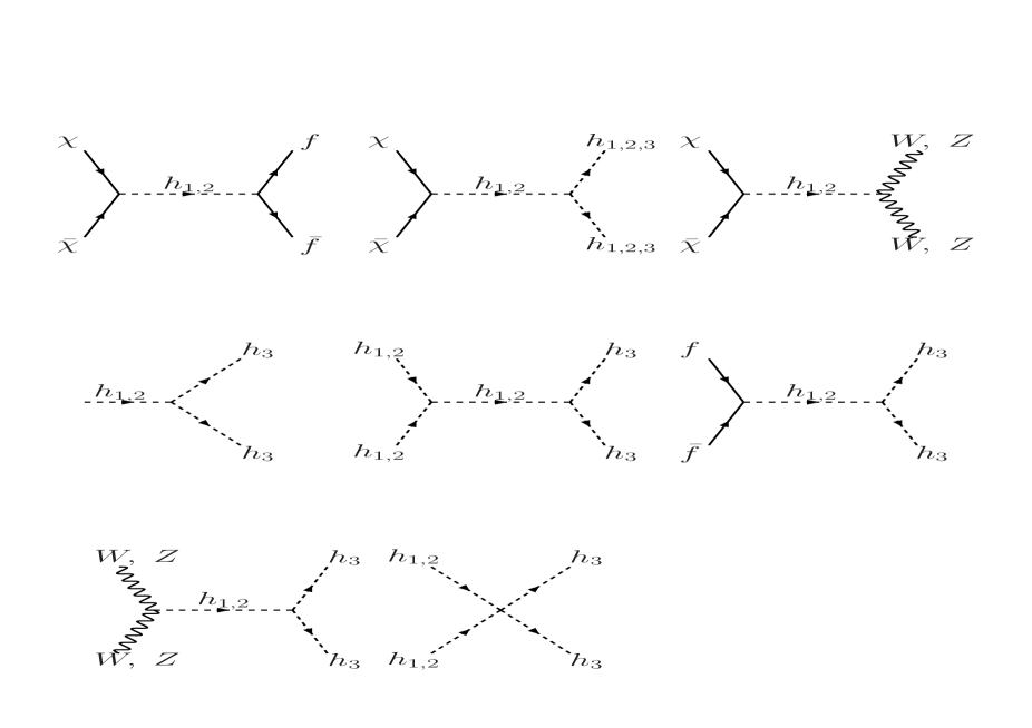
Figure 1: Feynman diagrams for the fermionic dark matter $\chi$ and scalar dark matter $h_{3}$

The relic density for the two component dark matter considered in the paper is obtained by solving the coupled Boltzmann equations for each of the dark matter components add then adding up the relic densities of each of the components.

The Boltzmann equation for the fermionic component $\chi$ in the present model is given by

$$\frac{dY_{\chi}}{dz} = -\langle\sigma v\rangle_{\chi\chi\rightarrow x\bar{x}}\left(Y_{\chi}^{2}-(Y_{\chi}^{\rm eq})^{2}\right)+\langle\sigma v\rangle_{\chi\chi\rightarrow h_{3}h_{3}}\left(Y_{\chi}^{2}-\frac{(Y_{\chi}^{\rm eq})^{2}}{(Y_{h_{3}}^{\rm eq})^{2}}Y_{h_{3}}^{2}\right)\,\,.$$ (23)

The fermionic dark matter in the present model follows usual freeze out mechanism and becomes relic which behaves as a WIMP dark matter. However, evolution of light dark matter $h_{3}$ is different. We assume that the mixing between the scalar $h_{j},j=1-3$ are very small. Therefore the scalar $h_{3}$ is produced from the decay or annihilation heavier particles such as Higgs or gauge bosons which never reaches thermal equilibrium (therefore becomes non-thermal in nature) and its production saturates as the Universe expands and cools down. This is also referred as freeze in production of particle [37, 38] and the light dark matter resembles a FImP like DM. Hence, initial abundance of $h_{3}$, $Y_{h_{3}}=0$ in the present model. Thus Eq. 23 takes the form

$$\frac{dY_{\chi}}{dz} = -\langle\sigma v\rangle_{\chi\chi\rightarrow x\bar{x}}\left(Y_{\chi}^{2}-(Y_{\chi}^{\rm eq})^{2}\right)+\langle\sigma v\rangle_{\chi\chi\rightarrow h_{3}h_{3}}Y_{\chi}^{2}\,\,,$$ (24)

where $x=f,\leavevmode\nobreak\ W,\leavevmode\nobreak\ Z,\leavevmode\nobreak\ h_{1},\leavevmode\nobreak\ h_{2}$, denotes the final state particles produced due to annihilation of dark matter candidate $\chi$. The Boltzmann equation for the scalar component $h_{3}$ in the present framework is given by

$$\frac{dY_{h_{{}_{{}_{3}}}}}{dz} = -\frac{2M_{pl}z}{1.66m^{2}}\frac{\sqrt{g_{\star}(T)}}{g_{\rm s}(T)}\Bigg{(}\sum_{i}\langle\Gamma_{h_{{}_{{}_{i}}}\rightarrow h_{{}_{{}_{3}}}h_{{}_{{}_{3}}}}\rangle\left(Y_{h_{{}_{{}_{3}}}}-{Y^{eq}_{h_{{}_{{}_{i}}}}}\right)\Bigg{)}\,-$$

$$\leavevmode\nobreak\ \frac{4\pi^{2}}{45}\frac{M_{pl}m}{1.66}\frac{\sqrt{g_{\star}(T)}}{z^{2}}\times$$

$$\Bigg{(}\sum_{x=W,Z,f,h_{1},h_{2}}\langle{\sigma{\rm v}}_{x\bar{x}\rightarrow h_{{}_{{}_{3}}}h_{{}_{{}_{3}}}}\rangle\,\,{({Y}^{2}_{h_{3}}}-{Y^{eq}_{x}\,{}^{2})}\,+\leavevmode\nobreak\ \langle{\sigma{\rm v}}_{\chi\chi\rightarrow h_{{}_{{}_{3}}}h_{{}_{{}_{3}}}}\rangle Y^{2}_{\chi}\Bigg{)}\,\,.$$

With $Y_{h_{3}}=0$, Eq. LABEL:bes takes the form

$$\frac{dY_{h_{{}_{{}_{3}}}}}{dz} = -\frac{2M_{pl}z}{1.66m^{2}}\frac{\sqrt{g_{\star}(T)}}{g_{\rm s}(T)}\Bigg{(}\sum_{i}\langle\Gamma_{h_{{}_{{}_{i}}}\rightarrow h_{{}_{{}_{3}}}h_{{}_{{}_{3}}}}\rangle\left(-{Y^{eq}_{h_{{}_{{}_{i}}}}}\right)\Bigg{)}\,-$$

$$\leavevmode\nobreak\ \frac{4\pi^{2}}{45}\frac{M_{pl}m}{1.66}\frac{\sqrt{g_{\star}(T)}}{z^{2}}\times$$

$$\Bigg{(}\sum_{x=W,Z,f,h_{1},h_{2}}\langle{\sigma{\rm v}}_{x\bar{x}\rightarrow h_{{}_{{}_{3}}}h_{{}_{{}_{3}}}}\rangle\,\,(-{Y^{eq}_{x}\,{}^{2})}\,+\leavevmode\nobreak\ \langle{\sigma{\rm v}}_{\chi\chi\rightarrow h_{{}_{{}_{3}}}h_{{}_{{}_{3}}}}\rangle Y^{2}_{\chi}\Bigg{)}\,\,.$$

In Eqs. 23-LABEL:bes1, $Y_{x}=\frac{n_{x}}{S}$ is the comoving number density of dark matter candidate $x=\chi,\leavevmode\nobreak\ h_{3}$ while $Y^{eq}_{x}$ is the equilibrium number density, $z=m/T$ where $T$ is the photon temperature and $S$ is the entropy of the Universe. $M_{pl}=1.22\times 10^{22}$ GeV in Eqs.  LABEL:bes-LABEL:bes1 denotes the Planck mass and the term $g_{\star}$ is expressed as [11]

$$\sqrt{{g_{\star}}(T)} = \frac{g_{S}(T)}{\sqrt{g_{\rho}(T)}}\left(1+\frac{1}{3}\frac{d\leavevmode\nobreak\ {\rm ln}g_{S}(T)}{d\leavevmode\nobreak\ {\rm ln}T}\right)$$ (27)

where $g_{S}$ and $g_{\rho}$ are the degrees of freedom corresponding to entropy and energy density of Universe and written as [11]

$$S=g_{S}(T)\frac{2\pi^{4}}{45}T^{3}\,,\hskip 15.0pt\rho=g_{\rho}(T)\frac{\pi^{2}}{30}T^{4}\,\,.$$ (28)

Thermal average of various annihilation cross-section ($\langle\sigma v\rangle$) and decay widths ($\langle\Gamma\rangle$) are given as

$$\langle\sigma{\rm v}\rangle_{aa\rightarrow bb} = \frac{1}{8m_{a}^{4}\,T\,K_{2}^{2}(m_{a}/T)}\int_{4m_{a}^{2}}^{\infty}ds\leavevmode\nobreak\ \sigma_{aa\rightarrow bb}(s)\leavevmode\nobreak\ (s-4m_{a}^{2})\,\sqrt{s}\,K_{1}(\sqrt{s}/T)$$

$$\langle\Gamma_{a\rightarrow bb}\rangle = \Gamma_{a\rightarrow bb}\frac{K_{1}(z)}{K_{2}(z)}\,\,.$$ (29)

In Eq. 29 $K_{1}$ and $K_{2}$ are modified Bessel functions and $s$ represents the centre of momentum energy. Using Eq. 24,LABEL:bes1 and Eqs. 27-29 we solve for the relic abundance of dark matter candidates given as

$$\Omega_{j}h^{2}=2.755\times 10^{8}\left(\frac{m_{j}}{GeV}\right)Y_{j}(T_{0}),\hskip 10.0ptj=\chi,h_{3}$$ (30)

where $T_{0}$ is the present photon temperature and $h$ is Hubble parameter expressed in the unit of 100 km s^-1 Mpc^-1. It is to be noted that relic densities of these two dark matter components must satisfy the condition for total dark matter density obtained from Planck [2] when added up, i.e.,

$$\Omega_{DM}h^{2}=\Omega_{\chi}h^{2}+\Omega_{h_{3}}h^{2}\,\,,\hskip 10.0pt0.1172\leq\Omega_{DM}h^{2}\leq 0.1226\,\,.$$ (31)

Expressions of different annihilation cross-sections and decay processes along with the relevant couplings are given in Appendix A. Feynman diagrams that contribute to the annihilations of $\chi$ along with the production of scalar dark matter $h_{3}$ via decay and annihilation channels are shown in Fig. 1. It is to be noted that the diagram $\chi\chi\rightarrow h_{3}h_{3}$ will also contribute to the production of light scalar dark matter.

4 Bounds from Collider Physics

ATLAS and CMS have confirmed their observation of a Higgs like scalar with mass $\sim$ 125.5 GeV [133, 134]. In the present model described in Sect. 2, we introduced three scalar particles. As mentioned earlier we assume $h_{1}$ as the Higgs like scalar and $h_{2}$ to be the non SM scalar ($85{\rm GeV}\leq m_{2}\leq 110$ GeV) while $h_{3}$ is the light dark matter candidate. Since $h_{1}$ is the Higgs like scalar with mass $\sim$ 125.5 GeV, we expect it to satisfy the collider bounds on signal strength of SM scalar. We define signal strength as

$$R_{1}=\frac{\sigma(pp\rightarrow h_{1})}{\sigma^{\rm SM}(pp\rightarrow h)}\frac{{\rm Br}(h_{1}\rightarrow xx)}{{\rm Br}^{\rm SM}(h\rightarrow xx)}\,\,.$$ (32)

In the above, $\sigma(pp\rightarrow h_{1})$ defines the production cross-section of $h_{1}$ due to gluon fusion while $\sigma^{\rm SM}(pp\rightarrow h)$ is the same for SM Higgs. Similarly ${\rm Br}(h_{1}\rightarrow xx)$ is defined as the decay branching ratio of $h_{1}$ into any final particle whereas the same for SM Higgs is ${\rm Br}^{\rm SM}(h\rightarrow xx)$. The Higgs like scalar must satisfy the condition for SM Higgs signal strength signal $R_{1}\geq 0.8$ [135]. Branching ratio to any final state particle for $h_{1}$ is given as ${\rm Br}(h_{1}\rightarrow xx)=\frac{\Gamma(h_{1}\rightarrow xx)}{\Gamma_{1}}$ (here $\Gamma(h_{1}\rightarrow xx)$ is decay width of $h_{1}$ into final state particles and $\Gamma_{1}$ is the total decay width of $h_{1}$) and for SM Higgs with mass 125.5 GeV it can be expressed as ${\rm Br}^{\rm SM}(h\rightarrow xx)=\frac{\Gamma(h\rightarrow xx)}{\Gamma_{SM}}$, where $\Gamma_{SM}$ is total decay width of Higgs. Hence, Eq. 32 can be written as

$$R_{1}=a_{11}^{4}\frac{\Gamma_{SM}}{\Gamma_{1}}$$ (33)

where $\Gamma_{1}=a_{11}^{2}\Gamma_{SM}+\Gamma^{inv}_{1}$ is the total decay width and $\Gamma^{inv}_{1}$ is the invisible decay width of $h_{1}$ into dark matter particles given as

$$\Gamma^{inv}_{1}=\Gamma_{h_{1}\rightarrow\chi\bar{\chi}}+\Gamma_{h_{1}\rightarrow h_{3}h_{3}}\,\,.$$ (34)

Similarly for $h_{2}$, the signal strength can be written as

$$R_{2}=a_{21}^{4}\frac{\Gamma^{\prime}_{SM}}{\Gamma_{2}}$$ (35)

with $\Gamma_{2}=a_{21}^{2}\Gamma^{\prime}_{SM}+\Gamma^{inv}_{2}$ respectively where $\Gamma^{\prime}_{SM}$ is the total decay width of non SM scalar of mass $m_{2}$ and $\Gamma^{inv}_{2}=\Gamma_{h_{2}\rightarrow\chi\bar{\chi}}+\Gamma_{h_{2}\rightarrow h_{3}h_{3}}$. The expression of invisible decay $\Gamma(h_{i}\rightarrow\chi\bar{\chi}),\leavevmode\nobreak\ i=1,2$ is

$$\Gamma_{h_{1}\rightarrow\chi\bar{\chi}}=\frac{m_{1}}{8\pi}g^{2}a_{21}^{2}\left(1-\frac{4m_{\chi}^{2}}{m_{1}^{2}}\right)^{1/2}\,\,,$$

$$\Gamma_{h_{2}\rightarrow\chi\bar{\chi}}=\frac{m_{2}}{8\pi}g^{2}a_{22}^{2}\left(1-\frac{4m_{\chi}^{2}}{m_{2}^{2}}\right)^{1/2}\,\,,$$ (36)

while the expression for $\Gamma_{h_{j}\rightarrow h_{3}h_{3}},\leavevmode\nobreak\ j=1,2$ are given in Appendix A. The invisible decay branching ratio for the SM like Higgs is $Br_{inv}^{1}=\frac{\Gamma_{1}^{inv}}{\Gamma_{1}}$. We assume the invisible decay branching ratio to be small and impose the condition $Br_{inv}^{1}<0.2$ [136].

5 Dark matter self interaction

Study of dark matter self interaction have recently received attention and have been explored in literatures [125, 126, 127]. Dark matter, though primarily thought to be collisionless in nature, is found to have self interaction from the observation of colliding galaxy clusters. A study of 72 colliding clusters by Harvey et. al. [126] claim that dark matter self interaction cross-section $\sigma_{DM}/m<0.47$ cm${}^{2}/$g with 95% CL. In the present model we proposed two dark matter candidates $\chi$ (WIMP like fermion) and a light scalar dark matter $h_{3}$ (FImP). In this work we will investigate whether any of these dark matter candidate can account for the observed dark matter self interaction cross-section. Study of dark matter self interaction by Campbell et. al. [128] have reported that a light dark matter with mass below 0.1 GeV produced by freeze in mechanism can provide the required amount of dark matter self interaction cross-section (contact interaction) in order to explain the observations of Abell 3827 [127] with $\sigma_{DM}/m\sim 1.5$ cm${}^{2}/$g which is close to the bound obtained from [126]. Therefore in the present work, we investigate whether the FImP dark matter $h_{3}$ (produced via freeze in mechanism as mentioned earlier in Sect. 3) can account for the dark matter self interaction cross-section given by [126, 127]. The ratio to self interaction cross-section with mass $m_{3}$ for the scalar dark matter candidate in the present model is given as [128]

$$\frac{\sigma_{h_{3}}}{m_{3}}=\frac{9\lambda_{3333}^{2}}{2\pi m_{3}^{3}}\,\,,$$ (37)

where $\lambda_{3333}$ is the quartic coupling for $h_{3}$ given in Appendix A. In the Eq. 37 we have considered contact interaction only and neglected the contributions from $s$-channel mediated diagrams since those are suppressed due to small coupling with scalars $h_{1}$ and $h_{2}$ and also due large mass terms in propagator.

5.1 3.55 keV X-ray emission and light dark matter candidate

Independent study of XMM Newton observatory data by Bulbul et. al. [94] and Boyarsky et. al. [95] have reported a 3.55 keV X-ray emission line from extragalactic spectrum. Such an observation can not be explained by known astrophysical phenomena. Although the signal is not confirmed, if it remains to exist then such a signature can be explained by decay of heavy dark matter candidates [110] or annihilation of light dark matter directly into photon [87, 109]. The observations from Hitomi collaboration [124] also suggests that the 3.55 keV X-ray line can be the caused by charge exchange phenomena in molecular nebula which requires more sensitive observation to be confirmed. Since in the present framework, we propose a light dark matter candidate $h_{3}$ to circumvent the self interaction property of dark matter, we further investigate whether it can also explain the 3.55 keV X-ray signal. For this purpose, we assume that mass of the light FImP dark matter candidate $h_{3}$ is $m_{3}\sim$ 7.1 keV which annihilate into pair of photons.

The expression for the decay of $h_{3}$ into 3.55 keV X-rays is given as

$$\Gamma_{h_{3}\rightarrow\gamma\gamma}=\left(\frac{\alpha_{\rm em}}{4\pi}\right)^{2}|F|^{2}\,\,a_{31}^{2}\,\frac{G_{F}m^{3}_{3}}{8\sqrt{2}\pi}\,\,,$$ (38)

where $G_{F}$ is the Fermi constant and $\alpha_{\rm em}\sim\frac{1}{137}$ is the fine structure constant. The loop factor $F$ in Eq. 38 is

$$F=F_{W}(\beta_{W})+\sum_{f}N_{c}Q_{f}^{2}F_{f}(\beta_{f})$$ (39)

where

$$\beta_{W} = \frac{4m_{W}^{2}}{m^{2}_{3}},\leavevmode\nobreak\ \leavevmode\nobreak\ \beta_{f}=\frac{4m_{f}^{2}}{m^{2}_{3}},$$

$$F_{W}(\beta) = 2+3\beta+3\beta(2-\beta)f(\beta),$$

$$F_{f}(\beta) = -2\beta[1+(1-\beta)f(\beta)],$$

$$f(\beta) = \arcsin^{2}[\beta^{-1/2}]\leavevmode\nobreak\ .$$

$N_{c}$ in the loop factor is the colour quantum number while $Q_{f}$ denotes the charge of the fermion. It is to be noted that the decay width of $h_{3}$ must be in the range $2.5\times 10^{-29}\leavevmode\nobreak\ {\rm s^{-1}}\leq f_{h_{3}}\Gamma_{h_{3}\rightarrow\gamma\gamma}\leq 2.5\times 10^{-28}\leavevmode\nobreak\ {\rm s^{-1}}$ in order to produce the required extragalactic X-ray flux obtained from Andromeda, Perseus etc. Since in the present model we have two dark matter components, the decay width of $h_{3}$ must be multiplied by a factor $f_{h_{3}}=\frac{\Omega_{h_{3}}}{\Omega_{DM}}$, is the fractional contribution to dark matter relic density by $h_{3}$ component. Hence, in this work we will also test the viability of the light scalar dark matter candidate to explain the possible X-ray emission signal reported by [94, 95] along with DM self interaction results.

6 Calculations and Results

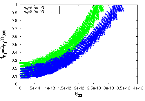
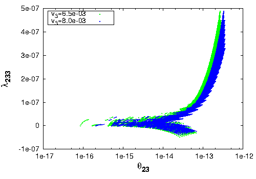
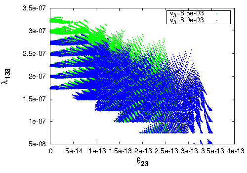
Figure 2: The left panel (Fig. 2a) shows the changes in $f_{h_{3}}$ with mixing angle $\theta_{23}$. Fig. 2b-c depicts the allowed values of the couplings $\lambda_{233}$ and $\lambda_{133}$ plotted against $\theta_{23}$.

$m_{1}$	$m_{2}$	$m_{3}$	$\lambda_{12}$	$\lambda_{13}$	$\lambda_{23}$	$R_{1}$	$Br_{inv}^{1}$	$f_{h_{3}}\Gamma_{h_{3}\rightarrow\gamma\gamma}$	$g$
GeV	GeV	GeV						10-29 s-1
$\sim$125.5	85-110	$\sim$7.1$\times$10-6	10-4-0.1	10-10-10-8	10-11-10-9	0.8-1.0	0-0.2	2.5-25	0.01-5.0

Table 1: Constraints and chosen region of model parameters space for the two component dark matter model.

In this section we test the viability of the present two component dark matter model scanning over a range of model parameter space. In Table 1, we tabulate the range of model parameter space and relevant constraints used in this work. Note that the coupling parameters $\lambda_{ij};\leavevmode\nobreak\ i,j=1-3,\leavevmode\nobreak\ (i\neq j)$ are in agreement with the vacuum stability conditions mentioned earlier in Eq. 22 (Sect. 2) and also satisfy perturbative unitarity condition. As we have mentioned earlier, $h_{1}$ is SM like scalar and $h_{2}$ is non SM scalar, we take $v_{1}=246$ GeV and $v_{2}=500$ GeV in the model. We further assume two choices of $v_{3}=$ 6.5 MeV and 8.0 MeV. This choice is consistent with the previous studies of light scalar dark matter of mass$\sim$7.1 keV with bound 2.0 MeV $\leq v_{3}\leq$ 10.0 MeV [87, 109]. We have also imposed the conditions on signal strength and invisible decay branching ratio of SM like scalar $h_{1}$ obtained from ATLAS and CMS at LHC ($R_{1}\geq 0.8$ and $Br_{inv}^{1}\leq 0.2$). Using the range of model parameter space tabulated in Table 1 we solve the three scalar mass mixing matrix in order to find out the elements of PMNS matrix $a_{ij};\leavevmode\nobreak\ i.j=1-3$ (and mixing angle). These matrix elements are then used to calculate various couplings mentioned in Appendix A which are necessary in order to calculate the decay widths and annihilation cross-sections of scalar dark matter candidate $h_{3}$. The coupling $g$ ($\leq 2\pi$, bound from perturbative limit) between the pseudo scalar and the fermionic dark matter is also varied within the range mentioned in Table 1 to compute the annihilation cross-sections for fermionic dark matter. These decay widths and annihilation cross-sections of both dark matter candidates are then used to solve for the coupled Boltzmann Eqs. 24,LABEL:bes1 and calculate the relic densities for each dark matter candidate satisfying the condition for total dark matter relic density Eq. 31. In Fig. 2 we show valid range of model parameter space obtained using Table 1 and solving the coupled Boltzmann equations satisfying the condition $\Omega_{\chi}h^{2}+\Omega_{h_{3}}h^{2}=\Omega_{DM}h^{2}$ as given by Planck satellite experiment. In Fig. 2a we plot the variation of allowed mixing angles $\theta_{23}$ with the fractional relic density $f_{h_{3}}$ of the scalar dark matter in the present framework . Plotted blue and green shaded regions depicted in all the three figures of Fig. 2 corresponds to the choice of $v_{3}=6.5\times 10^{-3}$ GeV and $8.0\times 10^{-3}$ GeV. The observation of Fig. 2a (in $\theta_{23}-f_{h_{3}}$ plane) shows that the relic density contribution of the scalar dark matter component increases with the increase in $\theta_{23}$. It is to be noted that the maximum allowed range of $\theta_{23}$ depends on the choice of $v_{3}$ and we have found that for $v_{3}=6.5\times 10^{-3}$ GeV $\theta_{23}^{max}\sim 2.8\times 10^{-13}$ while the same obtained with $v_{3}=8.0\times 10^{-3}$ GeV is $\theta_{23}^{max}\sim 3.5\times 10^{-13}$. This variation of $\theta_{23}$ with $f_{h_{3}}$ shown in Fig. 2a is a direct consequence of the fact that increase in $\theta_{23}$ also increases the value of $\lambda_{233}$ which is depicted in Fig. 2b. In Fig. 2b the variation of $\theta_{23}$ is plotted against $\lambda_{233}$. It is easily seen from Fig. 2b that when $\theta_{23}$ is small $\sim 10^{-16}-10^{-14}$, the value of $\lambda_{233}$ is very small. However as $\theta_{23}$ increase further, there is a sharp increase in the value of $|\lambda_{233}|$. As a result the contribution from the decay channel $h_{2}\rightarrow h_{3}h_{3}$ enhances which then also raises the relic density contribution of scalar $h_{3}$. From Fig. 2b we notice that maximum allowed range of $\lambda_{233}$ is $\sim 5\times 10^{-7}$ for both the cases of $v_{3}$ considered in the work. Finally in Fig. 2c $\theta_{23}$ is plotted against $\lambda_{133}$ for the both the values of $v_{3}$ mentioned above. From Fig. 2c we notice that $\lambda_{133}$ decreases steadily with enhancement in $\theta_{23}$ indicating an suppression in the contribution from $h_{1}$ (with $m_{1}\sim 125.5$ GeV) decay into pair of $h_{3}$. The allowed range of $\lambda_{133}$ for both the values of $v_{3}$ lie within the range $0.5\times 10^{-8}-3.5\times 10^{-7}$. In the present work mass of $h_{2}$ is varied in the range $85-110$ GeV (i.e., $m_{2}<m_{1}$) and decay width is inversely proportional to the mass of decaying particle (see Appendix A for expression). This indicates that the contribution of the non SM scalar to the freeze in production of FImP dark matter $h_{3}$ is significant compared to the same obtained from SM like scalar when coupling $\lambda_{233}$ is not small (i.e., $|\lambda_{233}|\sim\lambda_{133}$).

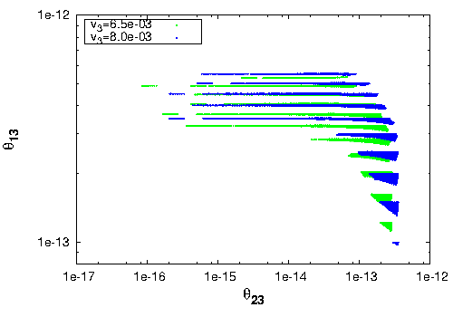
Figure 3: The available model parameter space in $\theta_{13}-\lambda_{133}$ plane is shown in the left panel (Fig. 3a) while in the right panel (Fig. 3b) the same region is depicted when $\theta_{23}$ is varied against $\theta_{13}$.

Fig. 3a depicts the allowed range of $\theta_{13}$ plotted against $\lambda_{133}$ for both the values of $v_{3}$ considered in earlier plots of Fig. 2. We also use the similar color scheme to indicate the values of $v_{3}$ satisfying the same conditions applied in order to plot Fig. 2. From Fig. 3a it can be easily observed that $\theta_{13}$ in the present model varies within the range $\sim 1.0-6.0\times 10^{-13}$ for both the chosen values of $v_{3}=6.5\times 10^{-3}$ GeV and $v_{3}=8.0\times 10^{-3}$ GeV respectively. It can also noticed from the plots in Fig. 3a that $\lambda_{133}$ is proportional to the value of $\theta_{13}$. This reveals that the decay width $h_{1}\rightarrow h_{3}h_{3}$ increases with increase in $\theta_{13}$ which can enhance the freeze in pair production of $h_{3}$ via $h_{1}$. In Fig. 3b we show the allowed model parameter space in $\theta_{23}-\theta_{13}$ plane for the same set of $v_{3}$ values and constrains used in earlier plots as well. Study of Fig. 3b reveals that for smaller values of $\theta_{23}\sim 10^{-16}-10^{-14}$, $\theta_{13}$ maintains a value in range $\sim 3\times 10^{-13}-6\times 10^{-13}$ indicating that contribution in the relic density is mostly contributed from the decay of $h_{1}$ into two $h_{3}$ scalars. However, as $\theta_{23}$ increase the contribution of $h_{2}$ increases (due to increase in $\lambda_{233}$) which reduces the value of $\theta_{13}$ (as well as $\lambda_{133}$) in order to maintain the contribution to total DM relic density by $h_{3}$ and to avoid overabundance of dark matter (when we add up the contribution on DM relic density obtained from the fermionic dark matter component $\chi$, i.e., $f_{h_{3}}+f_{\chi}=1$). It is to be mentioned that the mixing angles $\theta_{12}$ varies within the range $0.003\leq\theta_{12}\leq 0.183$ for the allowed model parameter space obtained using both set of $v_{3}$ considered. Note that all the plots in Fig. 2 and Fig. 3 are in agreement with the constraints on decay width of 7.1 keV scalar $h_{3}$ into X-ray, $2.5\times 10^{-29}$s${}^{-1}\leq f_{h_{3}}\Gamma_{h_{3}\rightarrow\gamma\gamma}\leq\leavevmode\nobreak\ 2.5\times 10^{-28}$s^-1. We have also found that the signal strength of $h_{2}$, i.e., $R_{2}$ in the present formalism is very small to be observed at the LHC experiments due to smallness of mixing between SM like scalar $h_{1}$ with $h_{2}$.

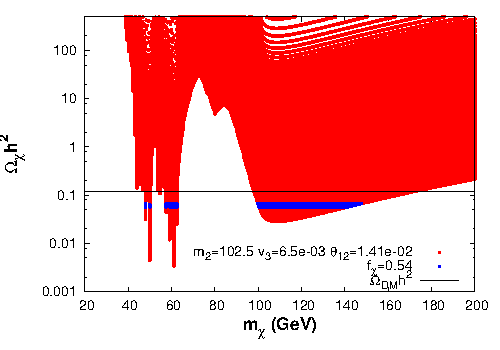
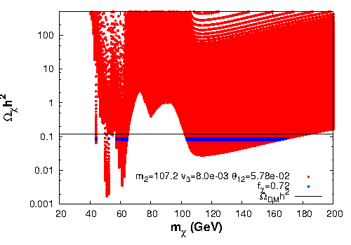
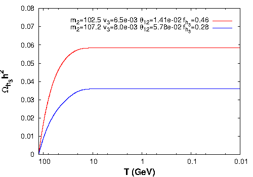
Figure 4: Plots in Fig. 4a-b shows the $m_{\chi}-\Omega_{\chi}h^{2}$ parameter space for the set of parameters in table 2 for the fermionic DM. The variation of $\Omega_{h_{3}}h^{2}$ (for the scalar DM $h_{3}$) with temperature $T$ for the same set of parameter is shown in Fig. 4c.

Set	$m_{1}$	$m_{2}$	$m_{3}$	$v_{3}$	$\theta_{12}$	$g$
	GeV	GeV	GeV	GeV
1	125.4	102.5	7.12$\times 10^{-6}$	6.5$\times 10^{-3}$	1.41$\times 10^{-2}$	0.01-5.0
2	125.5	107.2	7.15$\times 10^{-6}$	8.0$\times 10^{-3}$	5.78$\times 10^{-2}$	0.01-5.0

Table 2: Chosen parameter set for the plots in Fig. 4a-c.

So far, in this work, we have only discussed about the available parameters for the two component dark matter model involving a fermion $\chi$ and a light scalar $h_{3}$ of mass $\sim 7.1$ keV in agreement with Planck dark matter relic density satisfying the condition $\Omega_{\chi}h^{2}+\Omega_{h_{3}}h^{2}=\Omega_{DM}h^{2}$ (Fig. 2-3). In Fig. 4a-b we show the $m_{\chi}-\Omega_{\chi}h^{2}$ plots while in Fig. 4c the variation of dark matter density $\Omega_{h_{3}}h^{2}$ for light dark matter candidate $h_{3}$ ($m_{3}\sim 7.1$ keV) is plotted against the temperature $T$ of Universe. Instead of scanning over the full range of parameter space obtained from Fig. 2 and Fig. 3 (for two values of $v_{3}$), we consider two valid set of parameters for the purpose of demonstration tabulated in Table 2. Therefore, the parameter sets in Table 2 is within the range of scan performed using the Table 1 and also respects all other necessary conditions (such as vacuum stability, decay width of $h_{3}$, constrains from LHC etc.). Fermionic dark matter candidate can annihilate through $s$-channel annihilation mediated by scalars $h_{1}$ and $h_{2}$ (see Fig. 1). The mixing between the SM like scalar $h_{1}$ and non SM scalar $h_{2}$ given by $\theta_{12}$, is necessary to calculate the parameters $a_{ij},\leavevmode\nobreak\ i,j=1,2$ and different annihilations of the fermionic dark matter. Since in the present work the range of coupling $\lambda_{12}$ is larger compared to other couplings $\lambda_{23}$ and $\lambda_{13}$, the parameters $a_{ij},\leavevmode\nobreak\ i,j=1,2$ will dominantly be determined by $\theta_{12}$. This is also justified by the plots in Fig. 3b where $\theta_{23}$ is varied with $\theta_{13}$ showing these mixing angles are very small. Therefore, we have chosen two values of $\theta_{12}$ for two set of $v_{3}$ values given in Table 2. Note that we have also considered the same set of $v_{3}$ values of light scalar $S$ in our model along with $v_{1}=246$ GeV and $v_{2}=500$ GeV taken earlier in order to find out the valid range parameter space obtained in Figs. 2-3. Shown $m_{\chi}-\Omega_{\chi}h^{2}$ plot in Fig. 4a corresponds to the set of parameters with $v_{3}=6.5\times 10^{-3}$ GeV and the same with other set of parameters (when $v_{3}=8.0\times 10^{-3}$ GeV) is depicted in Fig. 4b. The red regions in both the Figs. 4a-b is obtained by varying the coupling $g$ within the range $0.01\leq g\leq 5.0$ and also varying the fermionic dark matter mass $m_{\chi}$ from 20 GeV to 200 GeV. From both the Figs. 4a-b it can be observed that a very small region of parameter space (for these chosen sets in Table 2) lies below the total dark matter density bound given by Planck [2] (black horizontal line shown in both the plots Fig. 4a-b). We have found that relic density of fermionic dark matter becomes less abundant with respect to total dark matter relic density near the resonances of SM like Higgs ($h_{1}$) and non SM scalar $h_{2}$ when its mass $m_{\chi}\sim m_{i}/2,\leavevmode\nobreak\ i=1,2$. Apart from that, there is also a region of parameter space with mass $\sim 100-180$ GeV (for $v_{3}=6.5\times 10^{-3}$ GeV) and $\sim 100-190$ GeV (when $v_{3}=8.0\times 10^{-3}$ GeV) where the condition $\Omega_{\chi}h^{2}<\Omega_{DM}h^{2}$ is satisfied. In this region the heavy fermionic dark matter annihilates into scalar $h_{1}$ and $h_{2}$. Thus the dark matter annihilation cross-section get enhanced which reduces the relic density $\Omega_{\chi}h^{2}$ of fermionic dark matter candidate. Shaded blue horizontal regions shown in the plot Fig. 4a (Fig. 4b) are fractional contributions to the total DM relic density from fermionic dark matter candidate $\chi$ with $f_{\chi}=0.54$ ($f_{\chi}=0.72$) where $f_{\chi}=\frac{\Omega_{\chi}}{\Omega_{DM}}$. In Fig. 4c we show the evolution of relic density $\Omega_{h_{3}}h^{2}$ of the light scalar dark matter $h_{3}$ as a function of temperature $T$ of the Universe with the same set of parameters given in Table 2. The plot shown in red (blue) depicted in Fig. 4a (Fig. 4b) corresponds to the parameter set with $v_{3}=6.5\times 10^{-3}$ GeV ($v_{3}=8.0\times 10^{-3}$ GeV). Moreover, we have also satisfied the condition $f_{\chi}+f_{h_{3}}=1$ in the plots of Fig. 4c (in order to produce the total DM relic abundance obtained from Planck results [2]) such that the fractional contribution of $h_{3}$ for each set of parameter in Table 2 is $f_{h_{3}}=1-f_{\chi}$, i.e., $f_{h_{3}}=0.46\leavevmode\nobreak\ (0.28)$ for the red (blue) plot depicted in Fig. 4c. It appears from the plots in Fig. 4c that the relic density of light scalar dark matter is very small (as initial abundance $Y_{h_{3}}=0$), increases gradually with decreasing temperature and finally saturates near $T\sim$ 10 GeV. The saturation of the relic density indicates that the production of $h_{3}$ ceases as the Universe expands and cools down due to rapid decrease in the number density of decaying or annihilating particles. Therefore from Fig. 4a-c it can be concluded that the present model of two component dark matter with a WIMP (heavy fermion $\chi$) and a FImP (light scalar $h_{3}$) can successfully provide the observed dark matter relic density predicted by Planck satellite data.

6.1 Direct detection of dark matter

In this section we will investigate whether the allowed model parameter space is compatible with the results from direct detection of dark matter obtained from dark matter direct detection experiments. Direct detection experiments search for the evidences of dark matter-nucleon scattering and provides bounds on dark matter-nucleon scattering cross-section. Dark matter candidates in the present model can undergo collision with detector nucleus and the recoil energy due to the scattering is calibrated. Since no such collision event have been observed yet by different dark matter direct detection experiments, these experiments provide an exclusion limit on dark matter-nucleon scattering cross-section. The most stringent bound on DM-nucleon spin independent (SI) cross-section is given by LUX [6], XENON-1T [7] and PandaX-II [8]. In the present model both the dark matter components (WIMP and FImP) $\chi$ and $h_{3}$ can suffer spin independent (SI) elastic scattering with the detector nucleus. The fermionic dark matter $\chi$ in the present work can interact through pseudo scalar interaction via $t$-channel processes mediated by both $h_{1}$ and $h_{2}$. The expression of spin independent scattering cross-section for the fermionic dark matter $\chi$ is

$$\sigma_{SI}^{\chi}=\frac{g^{2}}{\pi}m_{r}^{2}\left(\frac{a_{11}a_{12}}{m_{1}^{2}}+\frac{a_{22}a_{21}}{m_{2}^{2}}\right)^{2}\lambda_{p}^{2}\leavevmode\nobreak\ v^{2}$$ (40)

where $\lambda_{p}$ is given as [137]

$$\lambda_{p}=\frac{m_{p}}{v_{1}}\left[\sum_{q}f_{q}+\frac{2}{9}\left(1-\sum_{q}f_{q}\right)\right]\simeq 1.3\times 10^{-3}\,\,.$$ (41)

and $m_{r}=\frac{m_{\chi}m_{p}}{m_{\chi}+m_{p}}$ denotes the reduced mass for the scattering. It is to be noted that due to the pseudo scalar interaction scattering cross-section on Eq. 40 is velocity suppressed and hence multiplied by a factor $v^{2}\leavevmode\nobreak\$ with $v\sim 10^{-3}$ being the velocity of dark matter particle. We have found that this velocity suppressed scattering cross-section is way below the latest limit on DM-nucleon scattering given by Direct detection experiments [6]-[8] DM direct search experiment. This finding is also in agreement with the results obtained in a different work by Ghorbani [82]. Moreover, since we have two dark matter components in the model, the effective scattering cross-section for the fermionic dark matter (i.e., WIMP candidate) will be rescaled by a factor proportional to the fractional number density $r_{\chi}=\frac{n_{\chi}}{n_{\chi}+n_{h_{3}}}$ ($n_{x}$ denotes the number density), i.e., $\sigma_{SI}^{{}^{\prime}\chi}=r_{\chi}\sigma_{SI}^{\chi}$ (for further details see [84, 87]). The number density of both the dark matter components $\chi$ and $h_{3}$ can be obtained from the expression of individual relic density given in Eq. 30. In the present framework the fermionic dark matter candidate $\chi$ is $\sim 10^{6}$ times heavier than the scalar $h_{3}$ dark matter. For example if we consider that the contribution to the total relic density from $h_{3}$ is smaller with respect to that of fermion $\chi$ having value $\Omega_{h_{3}}h^{2}\sim 0.1\Omega_{\chi}h^{2}$, the number density of $h_{3}$ is $10^{6}$ times larger than that of $n_{\chi}$. This indicates that the rescaling factor $r_{\chi}\sim 10^{-6}$ and $r_{h_{3}}\sim 1$. Therefore the effective spin independent scattering cross-section $\sigma_{SI}^{{}^{\prime}\chi}$ for fermionic dark matter candidate is further suppressed by the rescaling factor $r_{\chi}<<1$ making it much smaller than the most sensitive dark matter direct detection limits obtained from experiments like LUX, PandaX-II. Similarly, for the scalar FImP dark matter candidate the effective spin independent direct detection cross-section is given as $\sigma_{SI}^{{}^{\prime}h_{3}}=r_{h_{3}}\sigma_{SI}^{h_{3}}$ where

$$\sigma_{SI}^{h_{3}}=\frac{m_{r}^{{}^{\prime}2}}{4\pi}\frac{f^{2}}{v_{1}^{2}}\frac{m_{p}^{2}}{m_{3}^{2}}\left(\frac{\lambda_{133}a_{11}}{m_{1}^{2}}+\frac{\lambda_{233}a_{21}}{m_{2}^{2}}\right)^{2}\,\,,$$ (42)

where $m^{\prime}_{r}=\frac{m_{3}m_{p}}{m_{3}+m_{p}}$ and $f\sim$0.3 [138]. Since $m_{3}<<m_{p}$, $m^{\prime}_{r}\sim m_{3}$ and Eq. 42 can be rewritten as

$$\sigma_{SI}^{h_{3}}=\frac{1}{4\pi}\frac{f^{2}}{v_{1}^{2}}m_{p}^{2}\left(\frac{\lambda_{133}a_{11}}{m_{1}^{2}}+\frac{\lambda_{233}a_{21}}{m_{2}^{2}}\right)^{2}\,\,.$$ (43)

Since $h_{3}$ in the present model has very small interaction with the SM bath particles and never reaches equilibrium after once produced, the couplings $\lambda_{133}$ and $\lambda_{233}$ are very small ($\sim 10^{-7}$, as seen from Fig. 2b-c). We have found that though the number density of $h_{3}$ is high $r_{h_{3}}\sim 1$ (as it is light), effective scattering cross-section $\sigma_{SI}^{{}^{\prime}h_{3}}\sim\sigma_{SI}^{h_{3}}$ is also very small to be observed by any dark matter direct search experiments and remains far below the most stringent limit given by LUX [6], XENON-1T [7] and PandaX-II [8] due to smallness of couplings $\lambda_{j33},\leavevmode\nobreak\ j=1,2$. Therefore, in the present scenario of two component dark matter model (with a WIMP and a FImP), we do not expect any bound on model parameter space from direct detection experimental constraints.

7 Galactic Centre gamma ray excess and dark matter self interaction

An excess of gamma ray in the energy range 1-3 GeV have been obtained from analysis of Fermi-LAT data [46] in the region of Galactic Centre. Such an excess can be interpreted as a result of dark matter annihilation in the GC region. Dark matter particles can be trapped due the immense gravitational pull of GC and also other astrophysical sites like dwarf galaxies, Sun etc. These sites are rich with particle dark matter which then undergo pair annihilation. Different particle physics models for dark matter are explored in order to provide a suitable explanation to this excess in gamma ray at GC as we have mentioned earlier in Sect. 1. An analysis of this 1-3 GeV GC excess gamma ray by Calore, Cholis and Weniger (CCW) [57] using various galactic diffusion excess models suggests that Fermi-LAT data can be explained by dark matter annihilation at GC. Indeed, the $\gamma$-ray excess can be very well fitted with a dark matter of mass $49^{+6.4}_{-5.4}$ GeV which annihilates into pair of $b\bar{b}$ particles with annihilation cross-section ${\langle\sigma v\rangle}_{b\bar{b}}=1.76^{+0.28}_{-0.27}\times 10^{-26}\leavevmode\nobreak\ {\rm cm}^{3}{\rm s}^{-1}$. In this section we will investigate whether the WIMP like fermionic dark matter candidate $\chi$ can account for the observed GC gamma ray excess results. In addition, self interaction study of the light scalar dark matter (FImP DM, mentioned earlier in Sect. 5) will also be addressed in this section. Before we explore the dark matter interpretation of GC gamma ray excess, a discussion is in order. The study of gamma ray signatures from dwarf galaxies by Fermi-LAT and DES [60, 61] also provide limits on dark matter annihilation cross-section into various annihilation modes. The limits on dark matter annihilation cross-section into $b\bar{b}$ is consistent with the GC gamma ray excess analysis by CCW. However, apart from dark matter annihilation, the gamma ray excess at GC in the range 1-3 GeV can also be explain by various non DM phenomena such as contribution from point sources near GC [58] or millisecond pulsars [59]. Study by Clark et. al. [139] also rule out the idea that the point like sources are dark matter substructures. However, in a recent work Fermi-LAT and DES collaboration have performed an analysis of $\gamma$-ray data with 45 confirmed dwarf spheroidals (dSphs) [62]. The analysis of gamma ray emission data from these dSphs by Fermi-LAT and DES provides bound on dark matter annihilation cross-section into different final channel particles ($b\bar{b}$ and $\tau\bar{\tau}$). Although their analysis [62] of the data do not show any significant excess at these sites (dSphs), the limits obtained on DM annihilation cross-section in their analysis do not exclude the possibility of DM interpretation of GC gamma ray excess either. Therefore in the present work, we will consider dark matter as the source to the gamma ray excess at Galactic Centre observed by Fermi-LAT and test the viability of our model.

BP1	$m_{1}$	$m_{2}$	$m_{\chi}$	$v_{3}$	$g$	$R_{1}$	$Br_{inv}^{1}$	$f_{\chi}$	$f_{\chi}^{2}{\langle\sigma v\rangle}_{b\bar{b}}$	$r_{\chi}$	$\sigma_{SI}^{{}^{\prime}\chi}$
	GeV	GeV	GeV	$10^{-3}$					10-26		pb
				GeV					cm3s-1
1	125.9	104.3	50.0	6.5	0.07	0.89	0.079	0.89	1.66	1.19e-06	2.39e-26
2	125.8	106.8	47.5	8.0	0.05	0.94	0.038	0.91	1.54	1.36e-06	1.15e-26

Table 3: Benchmark points for calculation of GC gamma ray excess plotted in Fig. 5 with fermionic dark matter $\chi$.

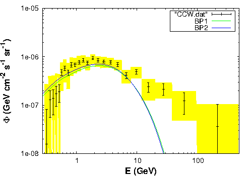
Figure 5: Comparison of the Fermi-LAT excess results from CCW [57] with the gamma ray flux obtained from benchmark points tabulated in Table 3.

BP1	$m_{1}$	$m_{2}$	$m_{3}$	$v_{3}$	$f_{h_{3}}$	$f_{h_{3}}\Gamma_{h_{3}\rightarrow\gamma\gamma}$	$r_{h_{3}}$	$\frac{\sigma_{h_{3}}}{m_{3}}$	$\sigma_{SI}^{h_{3}}$
	GeV	GeV	keV	$10^{-3}$		10-29		cm${}^{2}/$g	pb
				GeV		s-1
1	125.9	104.3	7.12	6.5	0.11	3.36	$\sim 1$	0.313	7.08e-24
2	125.8	106.8	7.15	8.0	0.09	5.06	$\sim 1$	0.137	7.15e-24

Table 4: Calculations of different observables for the scalar dark matter candidate for the same set of benchmark points given in Table 3.

The expression for the differential gamma ray flux obtained a region of Galactic Centre for the fermionic dark matter candidate $\chi$ is

$$\frac{\rm d^{2}\Phi}{\rm dEd\Omega}=\frac{{\langle\sigma{\rm v}\rangle}_{f}}{8\pi m_{\chi}^{2}}J\frac{dN^{f}_{\gamma}}{dE_{\gamma}}\,\,,$$ (44)

performed over a solid angle $d\Omega$ for certain region of interest (ROI). From Eq. 44, it can be observed that the differential $\gamma$-ray flux depends on the thermal averaged annihilation cross-section ${\langle\sigma v\rangle}_{f}$ of dark matter into final state particles (fermions) and $\frac{dN^{f}_{\gamma}}{dE_{\gamma}}$, is the photon energy spectrum produced due to per annihilation into fermions. In the above Eq. 44, the factor $J$, the astrophysical factor depending on the dark matter density $\rho$, is expressed as

$$J=\int_{\rm los}\rho^{2}(r(r^{\prime},\theta))dr\,\,,$$ (45)

is the line of sight integral where $r^{\prime}=\sqrt{r_{\odot}^{2}+r^{2}-2r_{\odot}r\cos\theta}$ with $r$ being the distance from the region of annihilation (GC) to Earth and $r_{\odot}=8.5$ kpc. The angle between line of sight and line from GC is denoted by $\theta$. In this work, we assume the dark matter distribution is spherically symmetric which follows Navarro-Frenk-White (NFW) [140] profile given as

$$\rho(r)=\rho_{s}\frac{(r/r_{s})^{-\gamma}}{(1+r/r_{s})^{3-\gamma}}\,.$$ (46)

In the expression of NFW halo profile $r_{s}=20$ kpc and $\rho_{s}$ is a typical scale density such that it produce the local dark matter density $\rho_{\odot}=0.4$ GeV cm^-3 at a distance $r_{\odot}$. The differential gamma ray flux is calculated using the ROI used in the work by CCW [57] ($|l|\leq 20^{0}$ and $2^{0}\leq|b|\leq 20^{0}$) for $\gamma=1.2$. The photon spectrum $\frac{dN^{f}_{\gamma}}{dE_{\gamma}}$ from the annihilation of dark matter is obtained from Cirelli [141]. In order to calculate the differential gamma ray flux obtained for the fermionic dark matter using Eqs. 44-46 and the specified ROI by CCW, we consider two benchmark points from the available model parameter space discussed earlier in Sect. 6. Therefore the benchmark points are in agreement with all the limits and constrains such as vacuum stability, LHC bounds, limits on decay width of light scalar, dark matter relic density etc. The benchmark points used to calculate gamma ray flux in this work is tabulated in Table 3. It is to be noted that since the dark matter candidate is fermion, one may think that the annihilation cross-section will be velocity suppressed. However, in the present model, the fermion dark matter has a pseudo scalar type interaction which removes the velocity dependence of dark matter annihilation cross-section [82]. In Fig. 5, we compare the GC gamma ray flux produced using benchmark points BP1 and BP2 tabulated in Table 3 with the results from CCW [57] for GC gamma ray excess. It is to be noted that the annihilation cross-section for the fermionic dark matter $\chi$ into $b\bar{b}$, i.e., ${\langle\sigma v\rangle}_{b\bar{b}}$ will be multiplied by $f_{\chi}^{2}$ (since annihilation requires two dark matter candidates). Hence in order to produce the required flux for excess GC gamma ray, the contribution to the relic density by the fermionic candidate $f_{\chi}$ should be large. In Fig. 5, the gamma ray flux obtained from BP1 (BP2) is plotted in green (blue) along with the data obtained from CCW [57]. From Fig. 5, it can be observed that the fermionic dark matter component $\chi$ (WIMP) in our model can account for the observed GC gamma ray excess results obtained by analysis of Fermi-LAT data. Moreover, from the benchmark points it can also be seen that the spin independent direct detection cross-section for the fermionic dark matter candidate calculated using Eqs. 40,41 is very small and remains below the limits from most stringent constraints on DM-nucleon cross-section given by LUX [6], XENON-1T [7] etc.

As we have mentioned earlier, we now investigate whether the light scalar dark matter $h_{3}$ can satisfy the condition for dark matter self interaction with the same set of benchmark points. The relevant results for the scalar dark matter candidate $h_{3}$ for BP1 and BP2 are tabulated in Table. 4. From Table. 4, it can be easily seen that for both the benchmark points, the light scalar dark matter can provide a self interaction cross-section consistent with the observed limits $\sigma/m\leq 0.47$ cm${}^{2}/$g obtained from the study by Harvey et. al. [126]. The self interaction for the light scalar DM candidate is calculated using Eq. 37.

It can also be seen from Table 4 that the FImP like scalar DM can also explain the 3.55 keV X-ray emission as observed by XMM Newton observatory if confirmed later as well. Calculation of DM-nucleon scattering cross-section for the scalar dark matter (using Eq. 43) also indicates that direct detection of the candidate is not possible at present having a small $\sigma_{SI}^{{}^{\prime}h_{3}}$ compared to the upper limit obtained LUX and other DM direct search experiments. Hence, at present, both the dark matter candidates ($\chi$ and $h_{3}$) are beyond reach of ongoing direct DM search experiments with spin independent scattering cross-section lying far below the existing limits obtained from these experiments. This justifies our previous comments on the scattering cross-section for the dark matter particles with detector nucleon discussed in Sect. 6.1.

8 Summary and conclusion

In this work we have explored the viability of a two component dark matter model with a fermionic dark matter that evolve thermally behaving like a WIMP and a non-thermal feebly interacting light singlet scalar dark matter which is produced via freeze in mechanism (FImP). The fermionic dark matter candidate $\chi$ interacts with the SM sector through a pseudo scalar particle $\Phi$ as the pseudo scalar acquires a non zero VEV and thus CP symmetry of the Lagrangian is broken spontaneously. Similarly the $\mathbb{Z}_{2}$ symmetry of the singlet scalar is also broken spontaneously when $S$ is given a tiny non-zero VEV resulting three physical scalars. However, the global $U(1)_{\rm DM}$ symmetry of the fermionic dark matter remains intact to provide us stable dark WIMP like DM candidate. On the other hand the light scalar $h_{3}$ having a very small interaction with SM sector also serves as a FImP dark matter candidate produced via freeze in mechanism. The $SU(2)_{\rm L}\times U(1)_{\rm Y}$ symmetry of SM Higgs field is also broken spontaneously which provide mass to the SM particles. Hence, in the present model we have three scalars which mix with each other. We identify one of the physical scalar $h_{1}$ to be SM like, $h_{2}$ as non SM Higgs and $h_{3}$ is the light scalar dark matter. We constrain the model parameter space by vacuum stability, unitarity, bounds from LHC results on SM scalar etc. to solve for the coupled Boltzmann equation in the present framework such that sum of relic densities of these dark matter candidates satisfy the observed DM relic density by Planck. We test for the viability of fermionic dark matter candidate in order to explain the GC gamma ray results obtained from the analysis of Fermi-LAT data [46] by CCW [57]. We show that excess of GC gamma ray in the energy range 1-3 GeV can be obtained from the annihilation of fermionic dark matter that produce the required amount of annihilation cross-section $\langle\sigma v\rangle_{b\bar{b}}$ having mass $\sim$ 50 GeV. There is also a valid region for the fermionic dark matter candidate $\chi$ with mass ranging from 100-190 GeV. In addition, we investigate whether the light scalar dark matter candidate can account for dark matter self interaction. We found that the light scalar dark matter $h_{3}$ considered in the model can provide the desired dark matter self interaction cross-section in order to explain the results from galaxy cluster collisions [126, 127]. Moreover, we also test for viability of this light dark matter candidate to explain the possible 3.55 keV X-ray signal obtained from the study of extragalactic X-ray emission reported by Bulbul et. al [94]. Our study reveals that a light dark matter $m_{3}\sim 7.1$ keV in the present model can serve as a viable candidate that produce the required flux (in agreement with the condition for decay width $h_{3}\rightarrow\gamma\gamma$) if confirmed by the observations of extragalactic X-ray search experiments and also consistent with the dark matter self interaction results. Both the dark matter candidates in the present “WIMP-FImP” framework are insensitive to direct detection experimental bounds and spin independent direct detection cross-section is far below the upper limit given by LUX DM direct search results. While this work is being completed, we came to know about a new work [142] on analysis of Fermi-LAT GC gamma ray excess for pseudo scalar interaction of dark matter using a different ROI ($15^{0}\times 15^{0}$) about GC with interstellar emission models (IEMs) and point sources. A detailed study of the results presented in [142] is beyond scope of this work and we wish to test these results for pseudo scalar interactions in our model in a future work.

Acknowledgments : Authors would like to thank P. Roy for his useful suggestions and valuable discussions.

Appendix A

• Annihilation cross-section of fermion dark matter candidate $\chi$

  $$\sigma{v}_{\chi\chi\rightarrow f\bar{f}} = N_{c}\frac{g^{2}}{32\pi}s\frac{m_{f}^{2}}{v_{1}^{2}}\left(1-\frac{4m_{f}^{2}}{s}\right)^{3/2}F(s,m_{1},m_{2})\,\,,$$

  $$\sigma{v}_{\chi\chi\rightarrow W^{+}W^{-}}=\frac{g^{2}}{64\pi}\left(1-\frac{4m_{W}^{2}}{s}\right)^{1/2}\left(\frac{m_{W}^{2}}{v_{1}}\right)^{2}\left(2+\frac{(s-2m_{W}^{2})^{2}}{4m_{W}^{4}}\right)F(s,m_{1},m_{2})\,\,,$$

  $$\sigma{v}_{\chi\chi\rightarrow ZZ}=\frac{g^{2}}{128\pi}\left(1-\frac{4m_{Z}^{2}}{s}\right)^{1/2}\left(\frac{m_{Z}^{2}}{v_{1}}\right)^{2}\left(2+\frac{(s-2m_{Z}^{2})^{2}}{4m_{Z}^{4}}\right)F(s,m_{1},m_{2})\,\,.$$

  $$F(s,m_{1},m_{2}) = \left[\frac{a_{12}^{2}a_{11}^{2}}{(s-m_{1}^{2})^{2}+m_{1}^{2}\Gamma_{1}^{2}}+\frac{a_{21}^{2}a_{22}^{2}}{(s-m_{2}^{2})^{2}+m_{2}^{2}\Gamma_{2}^{2}}\right.$$

  $$\left.+a_{12}a_{11}a_{22}a_{21}\frac{2(s-m_{1}^{2})(s-m_{2}^{2})+2m_{1}m_{2}\Gamma_{1}\Gamma_{2}}{[(s-m_{1}^{2})^{2}+m_{1}^{2}\Gamma_{1}^{2}][(s-m_{2}^{2})^{2}+m_{2}^{2}\Gamma_{2}^{2}]}\right]\,\,.$$

  $$\sigma{v}_{\chi\chi\rightarrow h_{1}h_{1}} = \frac{g^{2}}{32\pi}\left(1-\frac{4m_{1}^{2}}{s}\right)^{1/2}\left[\frac{a_{12}^{2}\lambda_{111}^{2}}{(s-m_{1}^{2})^{2}+m_{1}^{2}\Gamma_{1}^{2}}\right.$$

  $$\left.+\frac{a_{22}^{2}\lambda_{211}^{2}}{(s-m_{2}^{2})^{2}+m_{2}^{2}\Gamma_{2}^{2}}+\frac{2a_{12}a_{22}\lambda_{111}\lambda_{211}((s-m_{1}^{2})(s-m_{2}^{2})+m_{1}m_{2}\Gamma_{1}\Gamma_{2})}{[(s-m_{1}^{2})^{2}+m_{1}^{2}\Gamma_{1}^{2}][(s-m_{2}^{2})^{2}+m_{2}^{2}\Gamma_{2}^{2}]}\right]\,\,,$$

  $$\sigma{v}_{\chi\chi\rightarrow h_{2}h_{2}} = \frac{g^{2}}{32\pi}\left(1-\frac{4m_{2}^{2}}{s}\right)^{1/2}\left[\frac{a_{12}^{2}\lambda_{122}^{2}}{(s-m_{1}^{2})^{2}+m_{1}^{2}\Gamma_{1}^{2}}\right.$$

  $$\left.+\frac{a_{22}^{2}\lambda_{222}^{2}}{(s-m_{2}^{2})^{2}+m_{2}^{2}\Gamma_{2}^{2}}+\frac{2a_{12}a_{22}\lambda_{122}\lambda_{222}((s-m_{1}^{2})(s-m_{2}^{2})+m_{1}m_{2}\Gamma_{1}\Gamma_{2})}{[(s-m_{1}^{2})^{2}+m_{1}^{2}\Gamma_{1}^{2}][(s-m_{2}^{2})^{2}+m_{2}^{2}\Gamma_{2}^{2}]}\right]\,\,,$$

  $$\sigma{v}_{\chi\chi\rightarrow h_{3}h_{3}} = \frac{g^{2}}{32\pi}\left(1-\frac{4m_{3}^{2}}{s}\right)^{1/2}\left[\frac{a_{12}^{2}\lambda_{133}^{2}}{(s-m_{1}^{2})^{2}+m_{1}^{2}\Gamma_{1}^{2}}\right.$$

  $$\left.+\frac{a_{22}^{2}\lambda_{233}^{2}}{(s-m_{2}^{2})^{2}+m_{2}^{2}\Gamma_{2}^{2}}+\frac{2a_{12}a_{22}\lambda_{133}\lambda_{233}((s-m_{1}^{2})(s-m_{2}^{2})+m_{1}m_{2}\Gamma_{1}\Gamma_{2})}{[(s-m_{1}^{2})^{2}+m_{1}^{2}\Gamma_{1}^{2}][(s-m_{2}^{2})^{2}+m_{2}^{2}\Gamma_{2}^{2}]}\right]\,\,.$$

• Decay and annihilation terms for scalar dark matter candidate $h_{3}$

  $$\Gamma_{h_{{}_{{}_{j}}}\rightarrow h_{{}_{{}_{3}}}h_{{}_{{}_{3}}}} = \frac{\lambda^{2}_{j33}}{8\pi m_{j}}\sqrt{1-\frac{4m^{2}_{3}}{m^{2}_{j}}}\,\,,j=1,2\,\,,\leavevmode\nobreak\ \leavevmode\nobreak\ \leavevmode\nobreak\ \leavevmode\nobreak\ \leavevmode\nobreak\ \leavevmode\nobreak\ \leavevmode\nobreak\ \leavevmode\nobreak\ \leavevmode\nobreak\$$

  $$\sigma_{f\bar{f}\rightarrow h_{3}h_{3}}=N_{c}\frac{1}{16\pi s}\sqrt{(s-{4m_{3}^{2}})(s-4m_{f}^{2})}\left(\frac{m_{f}}{v_{1}}\right)^{2}F^{\prime}(s,m_{1},m_{2})\,\,,$$

  $$\sigma_{W^{+}W^{-}\rightarrow h_{3}h_{3}}=\frac{1}{18\pi s}\sqrt{\frac{s-{4m_{3}^{2}}}{s-4m_{W}^{2}}}\left(\frac{m_{W}^{2}}{v_{1}}\right)^{2}\left(2+\frac{(s-2m_{W}^{2})^{2}}{4m_{W}^{4}}\right)F^{\prime}(s,m_{1},m_{2})\,\,,$$

  $$\sigma_{ZZ\rightarrow h_{3}h_{3}}=\frac{1}{18\pi s}\sqrt{\frac{s-{4m_{3}^{2}}}{s-4m_{Z}^{2}}}\left(\frac{m_{Z}^{2}}{v_{1}}\right)^{2}\left(2+\frac{(s-2m_{Z}^{2})^{2}}{4m_{Z}^{4}}\right)F^{\prime}(s,m_{1},m_{2})\,\,.$$

  $$F^{\prime}(s,m_{1},m_{2}) = \left[\frac{a_{11}^{2}\lambda_{133}^{2}}{(s-m_{1}^{2})^{2}+m_{1}^{2}\Gamma_{1}^{2}}+\frac{a_{21}^{2}\lambda_{233}^{2}}{(s-m_{2}^{2})^{2}+m_{2}^{2}\Gamma_{2}^{2}}\right.$$

  $$\left.+a_{11}\lambda_{133}a_{21}\lambda_{233}\frac{2(s-m_{1}^{2})(s-m_{2}^{2})+2m_{1}m_{2}\Gamma_{1}\Gamma_{2}}{[(s-m_{1}^{2})^{2}+m_{1}^{2}\Gamma_{1}^{2}][(s-m_{2}^{2})^{2}+m_{2}^{2}\Gamma_{2}^{2}]}\right]\,\,.$$

  $$\sigma_{h_{1}h_{1}\rightarrow h_{3}h_{3}}=\frac{1}{2\pi s}\sqrt{\frac{s-{4m_{3}^{2}}}{s-4m_{1}^{2}}}\left(\lambda_{1133}+3\frac{\lambda_{111}\lambda_{133}}{(s-m_{1}^{2})}+\frac{\lambda_{211}\lambda_{233}}{(s-m_{2}^{2})}\right)^{2}\,\,.$$

  $$\sigma_{h_{2}h_{2}\rightarrow h_{3}h_{3}}=\frac{1}{2\pi s}\sqrt{\frac{s-{4m_{3}^{2}}}{s-4m_{2}^{2}}}\left(\lambda_{2233}+3\frac{\lambda_{222}\lambda_{233}}{(s-m_{2}^{2})}+\frac{\lambda_{122}\lambda_{133}}{(s-m_{1}^{2})}\right)^{2}\,\,.$$

• PMNS matrix with $\delta=0$

  $$U = \left(\begin{array}[]{ccc}c_{13}c_{12}&s_{12}c_{13}&s_{13}\\ -s_{12}c_{23}-s_{23}s_{13}c_{12}&c_{23}c_{12}-s_{23}s_{13}s_{12}&s_{23}c_{13}\\ s_{23}s_{12}-s_{13}c_{23}c_{12}&-s_{23}c_{12}-s_{13}s_{12}c_{23}&c_{23}c_{13}\end{array}\right)\,\,$$ (50)

• Couplings between different physical scalars obtained from the expression of potential

  $$-\lambda_{111} = \lambda_{H}v_{1}a_{11}^{3}+\lambda_{\Phi}v_{2}a_{12}^{3}+\lambda_{H\Phi}(v_{2}a_{11}^{2}a_{12}+v_{1}a_{11}a_{12}^{2})+\lambda_{HS}v_{1}a_{11}a_{13}^{2}+2\lambda_{\Phi S}v_{2}a_{12}a_{13}^{2}\,\,,$$

  $$-\lambda_{222} = \lambda_{H}v_{1}a_{21}^{3}+\lambda_{\Phi}v_{2}a_{22}^{3}+\lambda_{H\Phi}(v_{2}a_{21}^{2}a_{22}+v_{1}a_{21}a_{22}^{2})+\lambda_{HS}v_{1}a_{21}a_{23}^{2}+2\lambda_{\Phi S}v_{2}a_{22}a_{23}^{2}\,\,,$$

  $$-\lambda_{122} = 3\lambda_{H}v_{1}a_{11}a_{21}^{2}+3\lambda_{\Phi}v_{2}a_{12}a_{22}^{2}+\lambda_{H\Phi}(v_{2}(a_{21}^{2}a_{12}+2a_{11}a_{21}a_{22})+v_{1}(a_{11}a_{22}^{2}+2a_{21}a_{12}a_{22})$$

  $$+\lambda_{HS}v_{1}(a_{11}a_{23}^{2}+2a_{21}a_{13}a_{23})+2\lambda_{\Phi S}v_{2}(a_{12}a_{23}^{2}+2a_{22}a_{13}a_{23})\,\,,$$

  $$-\lambda_{211} = 3\lambda_{H}v_{1}a_{11}^{2}a_{21}+3\lambda_{\Phi}v_{2}a_{12}^{2}a_{22}+\lambda_{H\Phi}(v_{2}(a_{11}^{2}a_{22}+2a_{11}a_{21}a_{12})+v_{1}(a_{21}a_{12}^{2}+2a_{11}a_{12}a_{22})$$

  $$+\lambda_{HS}v_{1}(a_{21}a_{13}^{2}+2a_{11}a_{13}a_{23})+2\lambda_{\Phi S}v_{2}(a_{22}a_{31}^{2}+2a_{12}a_{13}a_{23})\,\,,$$

  $$-\lambda_{133} = 3\lambda_{H}v_{1}a_{11}a_{31}^{2}+3\lambda_{\Phi}v_{2}a_{12}a_{32}^{2}+\lambda_{H\Phi}(v_{2}(a_{31}^{2}a_{12}+2a_{11}a_{31}a_{32})+v_{1}(a_{11}a_{32}^{2}+2a_{31}a_{12}a_{32})$$

  $$+\lambda_{HS}v_{1}(a_{11}a_{33}^{2}+2a_{31}a_{13}a_{33})+2\lambda_{\Phi S}v_{2}(a_{12}a_{33}^{2}+2a_{32}a_{13}a_{33})\,\,,$$

  $$-\lambda_{233} = 3\lambda_{H}v_{1}a_{21}a_{31}^{2}+3\lambda_{\Phi}v_{2}a_{22}a_{32}^{2}+\lambda_{H\Phi}(v_{2}(a_{31}^{2}a_{22}+2a_{21}a_{31}a_{32})+v_{1}(a_{21}a_{32}^{2}+2a_{31}a_{22}a_{32})$$

  $$+\lambda_{HS}v_{1}(a_{21}a_{33}^{2}+2a_{31}a_{23}a_{33})+2\lambda_{\Phi S}v_{2}(a_{22}a_{33}^{2}+2a_{32}a_{23}a_{33})\,\,,$$

  $$-\lambda_{1133} = \frac{3}{2}(\lambda_{H}a_{11}^{2}a_{31}^{2})+\frac{3}{2}(\lambda_{\Phi}a_{12}^{2}a_{32}^{2})+\frac{3}{2}(\lambda_{S}a_{13}^{2}a_{33}^{2})+\frac{\lambda_{H\Phi}}{2}(a_{12}^{2}a_{31}^{2}+a_{11}^{2}a_{32}^{2}+4a_{11}a_{12}a_{31}a_{32})$$

  $$+\frac{\lambda_{HS}}{2}(a_{11}^{2}a_{33}^{2}+a_{13}^{2}a_{31}^{2}+4a_{11}a_{13}a_{31}a_{33})+\lambda_{\Phi S}(a_{12}^{2}a_{33}^{2}+a_{13}^{2}a_{32}^{2}+4a_{12}a_{13}a_{32}a_{33})\,\,,$$

  $$-\lambda_{2233} = \frac{3}{2}(\lambda_{H}a_{21}^{2}a_{31}^{2})+\frac{3}{2}(\lambda_{\Phi}a_{22}^{2}a_{32}^{2})+\frac{3}{2}(\lambda_{S}a_{23}^{2}a_{33}^{2})+\frac{\lambda_{H\Phi}}{2}(a_{22}^{2}a_{31}^{2}+a_{21}^{2}a_{32}^{2}+4a_{21}a_{22}a_{31}a_{32})$$

  $$+\frac{\lambda_{HS}}{2}(a_{21}^{2}a_{33}^{2}+a_{23}^{2}a_{31}^{2}+4a_{21}a_{23}a_{31}a_{33})+\lambda_{\Phi S}(a_{22}^{2}a_{33}^{2}+a_{23}^{2}a_{32}^{2}+4a_{22}a_{23}a_{32}a_{33})\,\,,$$

  $$-\lambda_{3333} = \frac{1}{4}(\lambda_{h}a_{31}^{4}+\lambda_{\Phi}a_{32}^{4}+\lambda_{S}a_{33}^{4})+\frac{\lambda_{H\Phi}}{2}a_{31}^{2}a_{32}^{2}+\frac{\lambda_{HS}}{2}a_{31}^{2}a_{33}^{2}+\lambda_{\Phi S}a_{32}^{2}a_{33}^{2}\,\,.$$

References

- [1] G. Hinshaw et al. [WMAP Collaboration], Astrophys. J. Suppl. 208, 19 (2013).
- [2] P. A. R. Ade et al. [Planck Collaboration], Astron. Astrophys. 571, A16 (2014).
- [3] Y. Sofue and V. Rubin, Ann. Rev. Astron. Astrophys. 39, 137 (2001).
- [4] M. Bartelmann and P. Schneider, Phys. Rept. 340, 291 (2001).
- [5] D. Clowe, A. Gonzalez and M. Markevitch, Astrophys. J. 604, 596 (2004).
- [6] D. S. Akerib et al., arXiv:1608.07648 [astro-ph.CO].
- [7] E. Aprile et al. [XENON Collaboration], JCAP 1604, no. 04, 027 (2016).
- [8] A. Tan et al. [PandaX-II Collaboration], Phys. Rev. Lett. 117, no. 12, 121303 (2016).
- [9] C. Amole et al. [PICO Collaboration], Phys. Rev. D 93, no. 5, 052014 (2016).
- [10] C. Amole et al. [PICO Collaboration], Phys. Rev. D 93, no. 6, 061101 (2016).
- [11] P. Gondolo and G. Gelmini, Nucl. Phys. B 360, 145 (1991).
- [12] M. Srednicki, R. Watkins and K. A. Olive, Nucl. Phys. B 310, 693 (1988).
- [13] G. Jungman, M. Kamionkowski and K. Griest, Phys. Rept. 267, 195 (1996).
- [14] V. Silveira and A. Zee, Phys. Lett. B 161, 136 (1985).
- [15] J. McDonald, Phys. Rev. D 50, 3637 (1994).
- [16] C. P. Burgess, M. Pospelov and T. ter Veldhuis, Nucl. Phys. B 619, 709 (2001).
- [17] V. Barger, P. Langacker, M. McCaskey, M. J. Ramsey-Musolf and G. Shaughnessy, Phys. Rev. D 77, 035005 (2008).
- [18] E. Ma, Phys. Rev. D 73, 077301 (2006).
- [19] L. Lopez Honorez, E. Nezri, J. F. Oliver and M. H. G. Tytgat, JCAP 0702, 028 (2007).
- [20] D. Majumdar and A. Ghosal, Mod. Phys. Lett. A 23, 2011 (2008).
- [21] M. Gustafsson, E. Lundstrom, L. Bergstrom and J. Edsjo, Phys. Rev. Lett. 99, 041301 (2007).
- [22] E. Lundstrom, M. Gustafsson and J. Edsjo, Phys. Rev. D 79, 035013 (2009).
- [23] S. Andreas, M. H. G. Tytgat and Q. Swillens, JCAP 0904, 004 (2009).
- [24] L. Lopez Honorez and C. E. Yaguna, JHEP 1009, 046 (2010).
- [25] L. Lopez Honorez and C. E. Yaguna, JCAP 1101, 002 (2011).
- [26] T. A. Chowdhury, M. Nemevsek, G. Senjanovic and Y. Zhang, JCAP 1202, 029 (2012).
- [27] D. Borah and J. M. Cline, Phys. Rev. D 86, 055001 (2012).
- [28] A. Arhrib, R. Benbrik and N. Gaur, Phys. Rev. D 85, 095021 (2012).
- [29] A. Goudelis, B. Herrmann and O. Stål, JHEP 1309, 106 (2013).
- [30] A. D. Banik and D. Majumdar, Eur. Phys. J. C 74, no. 11, 3142 (2014).
- [31] Y. G. Kim, K. Y. Lee and S. Shin, JHEP 0805, 100 (2008).
- [32] M. M. Ettefaghi and R. Moazzemi, JCAP 1302, 048 (2013).
- [33] M. Fairbairn and R. Hogan, JHEP 1309, 022 (2013).
- [34] T. Hambye, JHEP 0901, 028 (2009).
- [35] C. H. Chen and T. Nomura, Phys. Lett. B 746, 351 (2015).
- [36] S. Di Chiara and K. Tuominen, JHEP 1511, 188 (2015).
- [37] J. McDonald, Phys. Rev. Lett. 88, 091304 (2002).
- [38] L. J. Hall, K. Jedamzik, J. March-Russell and S. M. West, JHEP 1003, 080 (2010).
- [39] A. Merle and A. Schneider, Phys. Lett. B 749, 283 (2015).
- [40] A. Merle and M. Totzauer, JCAP 1506, 011 (2015).
- [41] B. Shakya, Mod. Phys. Lett. A 31, no. 06, 1630005 (2016).
- [42] A. Biswas and A. Gupta, JCAP 1609, no. 09, 044 (2016).
- [43] C. E. Yaguna, JHEP 1108, 060 (2011).
- [44] E. Molinaro, C. E. Yaguna and O. Zapata, JCAP 1407, 015 (2014).
- [45] A. Biswas and A. Gupta, arXiv:1612.02793 [hep-ph].
- [46] W. B. Atwood et al. [Fermi-LAT Collaboration], Astrophys. J. 697, 1071 (2009).
- [47] L. Goodenough and D. Hooper, [arXiv:0910.2998 [hep-ph]].
- [48] D. Hooper and L. Goodenough, Phys.Lett. B697 412 (2011).
- [49] A. Boyarsky, D. Malyshev, and O. Ruchayskiy, Phys.Lett. B705 165 (2011).
- [50] D. Hooper and T. Linden, Phys.Rev. D84 123005 (2011).
- [51] K. N. Abazajian and M. Kaplinghat, Phys.Rev. D86 083511 (2012).
- [52] D. Hooper and T. R. Slatyer, Phys.Dark Univ. 2 118 (2013).
- [53] K. N. Abazajian, N. Canac, S. Horiuchi, and M. Kaplinghat, Phys.Rev. D90 023526 (2014).
- [54] T. Daylan, D. P. Finkbeiner, D. Hooper, T. Linden, S. K. N. Portillo, N. L. Rodd and T. R. Slatyer, Phys. Dark Univ. 12, 1 (2016).
- [55] M. Ajello et al. [Fermi-LAT Collaboration], Astrophys. J. 819, no. 1, 44 (2016).
- [56] P. Agrawal, B. Batell, P. J. Fox and R. Harnik, JCAP 1505, 011 (2015).
- [57] F. Calore, I. Cholis, C. McCabe and C. Weniger, Phys. Rev. D 91, no. 6, 063003 (2015).
- [58] S. K. Lee, M. Lisanti, B. R. Safdi, T. R. Slatyer and W. Xue, Phys. Rev. Lett. 116, no. 5, 051103 (2016).
- [59] R. Bartels, S. Krishnamurthy and C. Weniger, Phys. Rev. Lett. 116, no. 5, 051102 (2016).
- [60] M. Ackermann et al. [Fermi-LAT Collaboration], Phys. Rev. Lett. 115, no. 23, 231301 (2015).
- [61] A. Drlica-Wagner et al. [Fermi-LAT and DES Collaborations], Astrophys. J. 809, no. 1, L4 (2015).
- [62] A. Albert et al. [Fermi-LAT and DES Collaborations], arXiv:1611.03184 [astro-ph.HE].
- [63] M. S. Boucenna and S. Profumo, Phys. Rev. D 84, 055011 (2011).
- [64] J. D. Ruiz-Alvarez, C. A. de S.Pires, F. S. Queiroz, D. Restrepo and P. S. Rodrigues da Silva, Phys. Rev. D 86, 075011 (2012).
- [65] N. Okada and O. Seto, Phys. Rev. D 89, no. 4, 043525 (2014).
- [66] A. Alves, S. Profumo, F. S. Queiroz and W. Shepherd, Phys. Rev. D 90, no. 11, 115003 (2014).
- [67] A. Berlin, D. Hooper and S. D. McDermott, Phys. Rev. D 89, 115022 (2014).
- [68] P. Agrawal, B. Batell, D. Hooper and T. Lin, Phys. Rev. D 90, 063512 (2014).
- [69] E. Izaguirre, G. Krnjaic and B. Shuve, Phys. Rev. D 90, 055002 (2014).
- [70] D. G. Cerdeño, M. Peiró and S. Robles, JCAP 1408, 005 (2014).
- [71] S. Ipek, D. McKeen and A. E. Nelson, Phys. Rev. D 90, 055021 (2014).
- [72] C. Boehm, M. J. Dolan and C. McCabe, Phys. Rev. D 90, 023531 (2014).
- [73] P. Ko, W. I. Park and Y. Tang, JCAP 1409, 013 (2014).
- [74] M. Abdullah, A. DiFranzo, A. Rajaraman, T. M. P. Tait, P. Tanedo and A. M. Wijangco, Phys. Rev. D 90, no. 3, 035004 (2014).
- [75] D. K. Ghosh, S. Mondal and I. Saha, JCAP 1502, no. 02, 035 (2015).
- [76] A. Martin, J. Shelton and J. Unwin, Phys. Rev. D 90, no. 10, 103513 (2014).
- [77] L. Wang and X. F. Han, Phys. Lett. B 739, 416 (2014).
- [78] T. Mondal and T. Basak, Phys. Lett. B 744, 208 (2015).
- [79] W. Detmold, M. McCullough and A. Pochinsky, Phys. Rev. D 90, 115013 (2014).
- [80] C. Arina, E. Del Nobile and P. Panci, Phys. Rev. Lett. 114, 011301 (2015).
- [81] N. Okada and O. Seto, Phys. Rev. D 90, no. 8, 083523 (2014).
- [82] K. Ghorbani, JCAP 1501, 015 (2015).
- [83] A. D. Banik and D. Majumdar, Phys. Lett. B 743, 420 (2015).
- [84] A. Biswas, J. Phys. G 43, no. 5, 055201 (2016).
- [85] K. Ghorbani and H. Ghorbani, Phys. Rev. D 93, no. 5, 055012 (2016).
- [86] D. G. Cerdeno, M. Peiro and S. Robles, Phys. Rev. D 91, no. 12, 123530 (2015).
- [87] A. Biswas, D. Majumdar and P. Roy, JHEP 1504, 065 (2015).
- [88] A. Achterberg, S. Amoroso, S. Caron, L. Hendriks, R. Ruiz de Austri and C. Weniger, JCAP 1508, no. 08, 006 (2015).
- [89] D. Borah, A. Dasgupta and R. Adhikari, Phys. Rev. D 92, no. 7, 075005 (2015).
- [90] A. Dutta Banik, D. Majumdar and A. Biswas, Eur. Phys. J. C 76, no. 6, 346 (2016).
- [91] B. Dutta, Y. Gao, T. Ghosh and L. E. Strigari, Phys. Rev. D 92, no. 7, 075019 (2015).
- [92] A. Cuoco, B. Eiteneuer, J. Heisig and M. Krämer, JCAP 1606, no. 06, 050 (2016).
- [93] A. Biswas, S. Choubey and S. Khan, JHEP 1608, 114 (2016).
- [94] E. Bulbul, M. Markevitch, A. Foster, R. K. Smith, M. Loewenstein and S. W. Randall, Astrophys. J. 789, 13 (2014)
- [95] A. Boyarsky, O. Ruchayskiy, D. Iakubovskyi and J. Franse, Phys. Rev. Lett. 113, 251301 (2014)
- [96] R. Krall, M. Reece and T. Roxlo, JCAP 1409, 007 (2014).
- [97] J. C. Park, S. C. Park and K. Kong, Phys. Lett. B 733, 217 (2014).
- [98] M. T. Frandsen, F. Sannino, I. M. Shoemaker and O. Svendsen, JCAP 1405, 033 (2014).
- [99] S. Baek and H. Okada, arXiv:1403.1710 [hep-ph].
- [100] K. Nakayama, F. Takahashi and T. T. Yanagida, Phys. Lett. B 735, 338 (2014).
- [101] K. Y. Choi and O. Seto, Phys. Lett. B 735, 92 (2014).
- [102] M. Cicoli, J. P. Conlon, M. C. D. Marsh and M. Rummel, Phys. Rev. D 90, no. 2, 023540 (2014).
- [103] C. Kolda and J. Unwin, Phys. Rev. D 90, 023535 (2014).
- [104] R. Allahverdi, B. Dutta and Y. Gao, Phys. Rev. D 89, 127305 (2014).
- [105] N.-E. Bomark and L. Roszkowski, Phys. Rev. D 90, no. 1, 011701 (2014).
- [106] S. P. Liew, JCAP 1405, 044 (2014).
- [107] K. Nakayama, F. Takahashi and T. T. Yanagida, Phys. Lett. B 734, 178 (2014).
- [108] E. Dudas, L. Heurtier and Y. Mambrini, Phys. Rev. D 90, 035002 (2014).
- [109] K. S. Babu and R. N. Mohapatra, Phys. Rev. D 89, 115011 (2014).
- [110] K. P. Modak, JHEP 1503, 064 (2015).
- [111] S. Baek, P. Ko and W. I. Park, arXiv:1405.3730 [hep-ph].
- [112] S. Chakraborty, D. K. Ghosh and S. Roy, JHEP 1410, 146 (2014).
- [113] C. W. Chiang and T. Yamada, JHEP 1409, 006 (2014).
- [114] B. Dutta, I. Gogoladze, R. Khalid and Q. Shafi, JHEP 1411, 018 (2014).
- [115] N. Haba, H. Ishida and R. Takahashi, Phys. Lett. B 743, 35 (2015).
- [116] J. M. Cline and A. R. Frey, JCAP 1410, no. 10, 013 (2014).
- [117] Y. Farzan and A. R. Akbarieh, JCAP 1411, no. 11, 015 (2014).
- [118] T. Higaki, N. Kitajima and F. Takahashi, JCAP 1412, no. 12, 004 (2014).
- [119] S. Patra, N. Sahoo and N. Sahu, Phys. Rev. D 91, no. 11, 115013 (2015).
- [120] K. S. Babu, S. Chakdar and R. N. Mohapatra, Phys. Rev. D 91, no. 7, 075020 (2015).
- [121] K. Cheung, W. C. Huang and Y. L. S. Tsai, JCAP 1505, no. 05, 053 (2015).
- [122] T. E. Jeltema and S. Profumo, Mon. Not. Roy. Astron. Soc. 450, no. 2, 2143 (2015).
- [123] E. Carlson, T. Jeltema and S. Profumo, JCAP 1502, no. 02, 009 (2015).
- [124] F. A. Aharonian et al. [Hitomi Collaboration], arXiv:1607.07420 [astro-ph.HE].
- [125] D. Harvey et al., Mon. Not. Roy. Astron. Soc. 441, no. 1, 404 (2014).
- [126] D. Harvey, R. Massey, T. Kitching, A. Taylor and E. Tittley, Science 347, 1462 (2015).
- [127] F. Kahlhoefer, K. Schmidt-Hoberg, J. Kummer and S. Sarkar, Mon. Not. Roy. Astron. Soc. 452, no. 1, L54 (2015).
- [128] R. Campbell, S. Godfrey, H. E. Logan, A. D. Peterson and A. Poulin, Phys. Rev. D 92, no. 5, 055031 (2015).
- [129] A. Biswas, D. Majumdar, A. Sil and P. Bhattacharjee, JCAP 1312, 049 (2013).
- [130] S. Bhattacharya, A. Drozd, B. Grzadkowski and J. Wudka, JHEP 1310, 158 (2013).
- [131] L. Bian, T. Li, J. Shu and X. C. Wang, JHEP 1503, 126 (2015).
- [132] A. Biswas, D. Majumdar and P. Roy, Europhys. Lett. 113, no. 2, 29001 (2016).
- [133] G. Aad et al. [ATLAS Collaboration], Phys. Lett. B 716, 1 (2012).
- [134] S. Chatrchyan et al. [CMS Collaboration], Phys. Lett. B 716, 30 (2012).
- [135] [ATLAS Collaboration], ATLAS-CONF-2012-162.
- [136] G. Belanger, B. Dumont, U. Ellwanger, J. F. Gunion and S. Kraml, Phys. Lett. B 723, 340 (2013).
- [137] L. Lopez-Honorez, T. Schwetz and J. Zupan, Phys. Lett. B 716, 179 (2012).
- [138] R. Barbieri, L. J. Hall and V. S. Rychkov, Phys. Rev. D 74, 015007 (2006).
- [139] H. A. Clark, P. Scott, R. Trotta and G. F. Lewis, arXiv:1612.01539 [astro-ph.HE].
- [140] J. F. Navarro, C. S. Frenk and S. D. M. White, Astrophys. J. 490, 493 (1997).
- [141] M. Cirelli, G. Corcella, A. Hektor, G. Hutsi, M. Kadastik, P. Panci, M. Raidal and F. Sala et al., JCAP 1103, 051 (2011).
- [142] C. Karwin, S. Murgia, T. M. P. Tait, T. A. Porter and P. Tanedo, arXiv:1612.05687 [hep-ph].