FADEWICH: Fast Deauthentication
over the Wireless Channel

Abstract

Both authentication and deauthentication are instrumental for preventing unauthorized access to computer and data assets. While there are obvious motivating factors for using strong authentication mechanisms, convincing users to deauthenticate is not straight-forward, since deauthentication is not considered mandatory. A user who leaves a logged-in workstation unattended (especially for a short time) is typically not inconvenienced in any way; in fact, the other way around – no annoying reauthentication is needed upon return. However, an unattended workstation is trivially susceptible to the well-known “lunchtime attack” by any nearby adversary who simply takes over the departed user’s log-in session. At the same time, since deathentication does not intrinsically require user secrets, it can, in principle, be made unobtrusive. To this end, this paper designs the first automatic user deauthentication system – FADEWICH – that does not rely on biometric- or behavior-based techniques (e.g., keystroke dynamics) and does not require users to carry any devices. It uses physical properties of wireless signals and the effect of human bodies on their propagation.

To assess FADEWICH’s feasibility and performance, extensive experiments were conducted with its prototype. Results show that it suffices to have nine inexpensive wireless sensors deployed in a shared office setting to correctly deauthenticate all users within six seconds (90% within four seconds) after they leave their workstation’s vicinity. We considered two realistic scenarios where the adversary attempts to subvert FADEWICH and showed that lunchtime attacks fail.

I Introduction

To prevent unauthorized access to various restricted resources, most computer systems mandate authentication and deauthentication mechanisms. Unfortunately, their efficacy is weakened since many users are too lazy, too distracted, or simply annoyed by these security procedures. Users who do not care about protecting resources (because they do not understand either their vaue or seriousness of threats) often attempt to avoid, circumvent or simplify security procedures, e.g., select easy-to-remember passwords [30] that are also easy to crack [5].

In most multi-user settings (e.g., home, office, school) most users tend to, perhaps grudgingly, accept the need for authentication. Moreover, mandatory system rules can dictate selection and change criteria, such that trivial passwords are avoided and new passwords are periodically required. However, since deauthentication requires no passwords (or any other secrets) easily annoyed, lazy or absent-minded users can leave their log-in session unattended, for numerous reasons, e.g., make a private phone-call, have a coffee, use the restroom or go to lunch. In this case, any physically nearby adversary can easily perform a so-called “lunchtime attack” [10], which basically means: walk up to the unattended computer and gain access to the current log-in session of the authorized departed user.

A great deal of prior research has been devoted to user authentication, yielding many techniques some of which are both effective (i.e., unavoidable), and usable, even transparent [1]. Currently, the most popular form of authentication involves providing traditional account credentials, i.e., username and password. At the same time, biometric-based techniques (e.g., fingerprint, voice, writing, iris, and face recognition) are gaining popularity both as stand-alone or second-factor means of authentication.

In contrast, much less attention has been paid to deauthentication. In particular, there is no effective (i.e., with low error rates) user-transparent deauthentication method. To the best of our knowledge, other than mandatory re-login after a fixed interval of user-input inactivity, there is no widely used deauthentication method. Unfortunately, if this interval is too short, users are annoyed by having to re-authenticate often and perhaps unnecessarily. Meanwhile, if it is too long, lunchtime attacks become more likely. In fact, lunchtime attacks are always possible when inactivity intervals are used: interval size determines the adversary’s window of opportunity.

Alternatively, explicit deauthentication can be mandated. It can be made very easy, e.g., just a single mouse click on a screen-lock icon. However, lazy, careless or distracted users neglect to follow the rules [23, 24]. Since username/password-based authentication will remain in wide use for the foreseeable future [12, 22], automatic deauthentication remains an open challenge. An ideal deathentication method would be unobtrusive (user-transparent) and highly effective.

Although lunchtime attacks involve physical constraints (i.e., the adversary must be physically near the victim), this is not an excuse to ignore the problem. In fact, insider attacks are very common and potentially very dangerous. For example, a 2014 survey of 557 large organizations showed that over half (53%) experienced an insider-caused security incident [7]. Also, average financial loss caused by such an incident exceeds US$100,000  [26]. Furthermore, as reported in 2015 by Verizon [31], insider and privilege misuse are the most frequent types of security incidents among 9 incident categories. Typically, malicious insiders exploit multiple opportunities throughout working hours to attempt to gain unauthorized access. Plus, being usually aware of local system vulnerabilities, they can act very quickly.

In this paper, we design a new deauthentication method, called Fast Deauthentication over the Wireless Channel (FADEWICH), which uses multiple wireless (WiFi) sensors deployed within an office. These devices communicate through the wireless radio channel and monitor physical properties of this channel. For actual deauthentication we take advantage of the effect that human bodies have on the propagation of high frequency wireless signals. Specifically, when a person crosses (or stands in) the path between a transmitter and a receiver, the body affects wireless signal propagation, such that the receiver measures the transmitted signal with a different strength, i.e., Received Signal Strength Indicator (RSSI) changes [33, 32]. A receiver determines signal strength of a wireless signal emitted by a transmitter by combining received signal components. In cluttered indoor environments (e.g., a typical office setting), signal strength is determined by components that arrive at the receiver after being scattered, reflected and diffracted by obstacles, such as walls and objects (multipath propagation). A person moving near wireless sensors causes signal components to change, producing fluctuations in measured signal strength, primarily by breaking the line-of-sight (LoS) condition between them, and by altering propagation of multipath signal components [19].

Contributions

This paper’s main contribution is a new deauthentication method – FADEWICH – suitable for a typical multi-user or shared office setting, where computers and workstations are not physically protected, e.g., by doors. In such a setting, a malicious insider can attempt to gain physical access to a workstation (or computer) that is left logged-in and unattended. FADEWICH is easy to deploy, user-transparent and does not require users to have any extra devices. FADEWICHis also efficient – it deauthenticates a user within a few seconds after stepping away – and usable, i.e., even idle users who remain at the workstation are not deauthenticated.

To assess feasibility and efficacy of FADEWICH, we implemented it and evaluated its performance in a realistic office setting. We designed and ran experiments with fewest possible assumptions: while users were aware of the system, they did not interact with it directly. Also, they were asked not to change their normal behavior, meaning that there are no limitations on how and how frequently they moved. We identified two realistic insider lunchtime attack scenarios We show that, with enough sensors, FADEWICH prevents all such lunchtime attacks. Moreover, we compare FADEWICH with simple time-out-based deauthentication and show that loss of usability in the former is negligible, especially considering security benefits that it offers.

II Related Work

We now overview wireless signal strength analysis for localization purposes (Section II-A), followed by state-of-the-art authentication and deauthentication techniques (Section II-B).

II-A RSSI for localization

Researchers have been using the effect of the human body on wireless signals for several years. Bahl et al. in their pioneering RADAR [2], used RSSI processing for localization purposes. RADAR was among the first works to consider the obstruction effect of the user body on the signal strengths, and thus point out the difference of the measured values between transceivers in LoS and not-LoS condition.

In wireless sensor networks, RSSI processing has been used for device free localization, where people can be located inside the monitored environment even if they do no carry a wireless enabled devices, using the body obstruction effect on the signals [15]. Kaltiokallio and Bocca [14] used this approach for intrusion detection. The system in [14], is able to detect and track the presence of an intruder who is moving inside the area monitored by wireless sensors. Further improvements were made, and RSSI processing was combined with Radio Tomographic Imaging (RTI) in order to track multiple people [4, 33]. RTI use a large number of wireless sensors to tackle the unpredictable nature of the radio environment: the information from several pairs of sensors is combined in order to infer the presence and movement of the person.

Although RTI techniques proved to be very effective to track people locations, these are not applicable in our context. In fact, in very cluttered and small rooms, the multipath components resulting from the reflections due to the walls, the objects, and the physical presence of users, have a fundamental role in the observed signal strength, producing very noisy and unpredictable changes [19]. Moreover, RTI is based on an initial calibration phase, where the system understands the behavior of the radio environment when there is nobody in it. Afterwards, the fluctuations caused by the movement of users result different compared to the learned behavior. In our model a static and long-term calibration is not possible, since there is not an unique “steady state”: the environment is dynamic, users may be walking inside the office, standing still, or sitting in their chairs.

II-B Deauthentication Solutions

Since the deauthentication strongly depends on the authentication scheme, an overview on these authentication mechanisms is necessary. Nowadays, the most popular authentication scheme is the use of passwords. Using passwords for the authentication has several advantages: they are very intuitive and convenient to use, users do not need to perform any activity (after the log in) nor carry any device. However, one of their main drawbacks is that there is no way of automatically deauthenticate users, exposing the user accounts and the system to possible threats. Security researchers have thoroughly pointed out the weaknesses of password-based authentication [5, 22, 6, 12], and they have invested lots of effort in the search for usable and secure alternatives.

In this direction, a promising field is behavioral biometrics. Behavioral biometrics are typically passive (or transparent) to the users, and can be used for continuous authentication. With continuous authentication techniques, the user is continuously authenticated as long as he interacts with the system, and he is deauthenticated once his interactions stop, providing automatic deauthentication. One of the more popular biometrics in this category is keystroke dynamics [3]. Even if these biometrics reached low error rates [11], and are approaching a wider adoption, their security guarantees remain questionable. In fact, error rates does not thoroughly represent the security properties of a biometric system: they only shows the resilience against the zero-effort attack (i.e., the success rate of one malicious user enrolled into the system that claims another user identity). When the threat model changes, the error rates could become irrelevant. For example, Meng et al. [28] have examined the reliability of the keystroke dynamics, and they showed that an adversary is able to reproduce one user behavior after a brief training (after observing the user typing on a keyboard). Recently, more sophisticated biometrics like the ones based on the pulse response [21], or on the eye movements [10, 25] have been investigated. Although these solutions are harder to observe and to craft by an adversary, their deployment requires specific hardware, which may be considerably expensive, and that hinders their large-scale adoption.

Another approach to the deauthentication, is to adopt techniques based on proximity. In these techniques, users carry small tokens that communicate over a short range radio channel with the workstations, providing continuous authentication [8, 27]. The workstations periodically poll the tokens via a secure channel to detect their proximity, and they are automatically secured as soon as the token is unreachable. The major drawback of proximity based authentication is that it requires the user to carry some device (and the system administrator to deploy and manage them), exposing to serious threats in case such devices are stolen.

Mare et al. proposed ZEBRA [16], an hybrid approach for the continuous authentication. In their work, they have users wear a bracelet with an in-built gyroscope on their dominant wrist, and they combine the inputs received on the workstation (i.e., mouse movement and keyboard typing) with the actions observed by the bracelet. Where the two time series of events do not correlate, the user is logged out and the workstation is locked. However, as pointed out by Huhta et al [13], ZEBRA design is flawed: they showed that 40% of attackers are able to remain logged in for more than 10 minutes by opportunistically choosing the time and type of interactions (bracelet and mouse movement, and keyboard typing). The authors acknowledge that the system relies on assumptions that makes it vulnerable to attackers, and even if ZEBRA performs well against accidental misuse by innocent users, opportunistic attackers remain a tough challenge.

III System Model

Our main goal is to automatically deauthenticate users who are logged into a workstation when they leave its proximity. The method must be inexpensive and easy to deploy with minimal (preferably none) hardware requirements. Another goal is usability which translates into user transparency and low error rates. An error refers to a false positive, i.e., a user being mistakenly deauthenticated while still using, and being physically present at, the workstation, thus forcing a superfluous log-in ( as discussed in [22], users find repetitive password entry time-consuming and very annoying). Also, the system must not invade user privacy, e.g., using a camera is obtrusive and generates privacy issues that might discomfit users [18]).

The system model is as follows:

1. The environment is a workplace with $k$ workstations $w_{1},$ $...,$ $w_{k}$. Users log in using some authentication mechanism the particulars of which are not important for deauthentication. Each workstation monitors user input activity and communicates the idle time to a central station. We assume that there is a single entrance – the only way users can access and exit the office.

2. There are $m$ wireless devices $d_{1},$ $...,$ $d_{m}$ each capable of sending packets and monitoring signal strength of packets received from the others. This lets us obtain $m\times(m-1)$ streams of signal strengths, which are transmitted through a secure channel (not necessarily a wireless one) to a central station.

3. At installation time, there is an initial phase when the system automatically collects and labels data. No adversarial presence is assumed during this phase.

III-A Threat Model

In the context of this paper, a threat means unauthorized access to an honest user’s account. We assume that the adversary is potentially anyone who has physical access to the office, e.g., co-workers, supervisors, customers, janitors, and delivery personnel. The adversary’s goal is to gain access to an active log-in session on the target workstation used by one victim user. The adversary does not know that user’s login credentials. We distinguish between two sub-types of adversaries:

• Insider: anyone with access to the outside of the office. This can be any employee of the same organization. However, insider is not supposed to enter the actual office housing the target workstation.

• Co-worker: anyone with access to the inside of the office (e.g., a co-worker, assigned to another workstation in the same office) who is not supposed to use the target workstation.

Since workstations might be close to each other, co-worker can access the target faster than insider. If automatic deauthentication is based on a fixed time-out, co-worker has a significant advantage.

As for other types of attacks, Section V-C discusses our reasons for not considering attacks that alter the physical propagation of wireless signals. We also do not consider social engineering attacks.

IV System Design

We now present technical details of FADEWICH and motivate its design.

IV-A Overview

The complete system includes several components and three main modules: Keyboard/Mouse Activity module (KMA, described in Section IV-B), Movement Detection module (MD, described in Section IV-C), and Radio Environment module (RE, described in Section IV-D). These modules can access information provided by sensors and workstations, and a classifier that has been previously trained (see Section IV-D3). Another component implements the control part of the system, which merges information provided by the modules to apply actions to the workstations. Section IV-E discusses the overlapping movements problem, while Section IV-F illustrates system actions and the workflow of FADEWICH.

Figure 1: Overview of FADEWICH components.

IV-B Keyboard/Mouse Activity (KMA)

This module monitors user input at each workstation, and keeps track of idle time, i.e., the interval of time the workstation observed no keyboard or mouse input. When the system at time $t$ asks KMA which workstations have been idle for $s$ seconds, KMA returns a set of workstations $S_{t}^{(s)}=\{w_{h},\>...,\>w_{j}\}$ that have been idle between $t-s$ and $t$.

IV-C Movement Detection (MD)

This module obtains signal strength streams and determines whether there has been any significant fluctuations in the radio environment. In the following, after introducing the notation, we show how such fluctuations are identified based on the discrepancy with a learned level of fluctuations.

IV-C1 Notation

We refer to signal strength measurement on stream $i$ at time $t$ as: $r_{t}^{(i)}$. A window on a stream is a sequence of measurements, such that, for a given size $d$, and time $t$:

$$V_{t-d,t}^{(i)}=\{r_{t-d}^{(i)},r_{t-d+1}^{(i)},...,r_{t}^{(i)}\}.$$

Given a distribution $r=\{r_{1},r_{2},...,r_{n}\}$, and a kernel function $K$, we refer to its estimated density function as:

$$\hat{f}_{K}(r)=\frac{1}{nh}\sum\limits_{i=1}^{n}K(\frac{r-r_{i}}{h}),$$

where $h$ is the bandwidth of the kernel.

IV-C2 Standard Deviation Profile

To recognize users’ movements, we decided to use the sum of the standard deviations of signal streams. Initially, MD builds a distribution of these summations, using a sliding window to compute standard deviations of some period of data, e.g., 30 seconds in our experiments. At each time step $t$, the summation of standard deviations $s_{t}$ is computed as:

$$s_{t}=\sum\limits_{i}\sigma_{V_{t-d,t}^{(i)}}\>\>,$$

where $\sigma_{V_{t-d,t}^{(i)}}$ is the standard deviation of measurements in window $V_{t-d,t}^{(i)}$, $d$ is window size, and $i$ identifies the stream. These values form a frequency distribution $s=\{s_{0},s_{1},...,s_{n}\}$, that we refer to as the normal profile. Density of distribution $s$ is estimated with a Gaussian kernel and the estimated function $\hat{s}$ is later used for comparison.

Thereafter, MD periodically computes the current sum of standard deviations $s_{t}$ with the latest observed data. When $s_{t}$ exceeds the $(100-\alpha)^{th}$ percentile of cumulative distribution function $\hat{S}$ of estimated distribution $\hat{s}$, the module reports the anomalous changes observed. When changes belong to the remaining part of the distribution, MD reports the normal state. Figure 2 shows the difference between the measurements of $s_{t}$ when no one is walking in the office, and when a user is walking inside. The solid line shows the probability distribution function estimated with the Gaussian kernel.

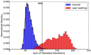
Figure 2: Frequency distribution of observed total standard deviation.

IV-C3 Profile Update

Due to the noisy nature of the radio environment, behavior of the streams varies slightly depending on several factors, in particular, the number of users in the room. To account for this phenomena, the normal profile needs to be updated with most recent measurements. We use batches of size $b$ for the update: each time current $s_{t}$ is computed, it is queued for the update. When the queue reaches size $b$, if less than a fraction $\tau$ of values in the queue belonged to $(100-\alpha)^{th}$ percentile of $\hat{S}$, they are added to the normal profile distribution by removing the oldest $b$ values. The kernel density estimation is performed again after each update.

Algorithm 1 shows MD workflow. Whenever MD returns anomalous, the current state of the environment significantly differs from the learned profile. Whereas, if it returns normal, the current state matches the profile.

Algorithm 1 MD workflow

1: $\hat{s}\leftarrow$ initialize_normal_profile()

2: $Q\leftarrow\{\}$ // batch for profile update

3:while True do

4:    $s_{t}\leftarrow\sum\limits_{i}\sigma_{V_{t-d,t}^{(i)}}$

5:    $ub\leftarrow\hat{S}^{(100-\alpha)^{th}}$

6:    $Q\leftarrow Q+\{s_{t}\}$

7:    if $s_{t}\geq ub$ then

8:         return anomalous

9:    else

10:         if $|Q|\geq b$ then

11:             if not is_anomalous(Q, $\tau$) then

12:                 $\hat{s}\leftarrow update\_distribution(\hat{s},Q)$

13:             else

14:                 $Q\leftarrow\{\}$

15:             end if

16:         end if

17:         return normal

18:    end if

19:end while

IV-C4 Variation Windows

Hereafter, we refer to variation windows as time intervals $[t_{1},t_{2}]$, where MD has recognized anomalous fluctuations that started at time $t_{1}$ and continued until $t_{2}$, when the the environment went back to normal. Unfortunately, user movements are not the only cause of fluctuations. The radio environment is subject to other uncontrolled changes that may result in variation windows even if no one is moving. To account for this possibility and to exclude other brief variations due to users moving slightly while remaining at their workstations, there is a threshold on the duration of variations windows $t_{\Delta}$. This way, variation windows shorter that $t_{\Delta}$ are ignored, while longer windows are interpreted as user movements and trigger a system decision. The value of $t_{\Delta}$ must be chosen very carefully, since it bears much impact on overall performance; see Section VII-A.

IV-D Radio Environment (RE)

The radio environment module reads the signal strength streams, and matches the observed signal changes to a specific workstation. A user who steps away from the workstation alters signal propagation of wireless sensors, based on trajectory of movement. These signal alterations form a recognizable pattern and we use a classifier to identify them. We now describe how training samples are built and labeled, as well as how the system is trained.

IV-D1 Samples

Each sample represents a signature of the effect on the radio environment of a user who after sitting at a workstation leaves the proximity of that workstation.

To obtain a sample, we need to identify the correct interval where the user leaves the proximity of the workstation. We use the timings provided by the variation windows measured by MD module, assuming that movement is always obtained with a variation window $[t_{1},t_{2}]$. When such a window is observed, for each stream $i$, we extract signal strengths observed in window:

$$V_{t_{1},t_{1}+t_{\Delta}}^{(i)}=\{r^{(i)}_{t_{1}},r^{(i)}_{t_{1}+1}...,r^{(i)}_{t_{1}+t_{\Delta}}\}$$

of size $|V_{t_{1},t_{1}+t_{\Delta}}^{(i)}|=n$, and we compute the following features:

• Variance of the window:

  $$\sigma^{2}=\frac{\sum\limits_{j}(r_{j}-\mu)^{2}}{n}.$$

• Entropy of the frequency distribution histogram $V$ of the window:

  $$H=-\sum\limits_{r_{j}\in V}P(r_{j})\log P(r_{j}).$$

• Autocorrelation of the window:

  $$R(k)=\frac{1}{(n-k)\sigma^{2}}\sum\limits_{j=t_{1}}^{n-k}(r_{j}-\mu)(r_{j+k}-\mu).$$

We use the window from $[t_{1},t_{1}+t_{\Delta}]$ instead of the full $[t_{1},t_{2}]$ because the most distinctive part of the user’s physical position when leaving the workstation occurs at the beginning. Some portions of the user’s path out of the office are likely to overlap with paths of other users (since there is a single door, users likely move towards it). Meanwhile, initial segments of users’ paths are naturally less likely to overlap.

IV-D2 Labels

We use a set of labels $w_{0},\>w_{1},\>...,\>w_{k}$ for samples associated with specific events. $w_{0}$ is associated with the event: “user entered the office” and each other $w_{i}$ is associated with the event: “user left workstation $w_{i}$”. $w_{0}$ is needed since users entering the office generate significant fluctuations in the radio environment: this must be detected so as not to mistakenly deauthenticate users who are still at their workstations.

IV-D3 Training Phase

During the training phase, FADEWICH runs the MD module to detect variation windows. For every variation window, FADEWICH extracts the corresponding sample, computing its features. Afterwards, the system uses KMA to fetch idle time for the workstations, and tries to automatically label the sample. The time of a user’s departure from the workstation and idle time at that workstation are correlated, since from the moment the user walks away the workstation observes no further input, until the user returns. To avoid erroneous labeling, when FADEWICH is uncertain (i.e., more than one workstation is idle during the variation window) it simply discards the sample. At the end of the training phase, labeled samples are used to set up a Support Vector Machine (SVM) classifier used in the online phase.

IV-D4 Online Phase

In this phase, whenever MD observes a variation window $W=[t_{1},t_{2}]$ of size $\geq t_{\Delta}$, at time $t_{1}+t_{\Delta}$ (before the end of the window) the system queries RE. The module fetches the window of signal strength measurements $V^{(i)}_{t_{1},t_{1}+t_{\Delta}},\forall\>i$, computes the features for the windows to construct the sample, inputs the sample into the classifier and returns the predicted label.

IV-E Overlaps

FADEWICH  does not recognize situations when multiple users walk away from their workstation at the same time, or their movement intervals overlap. RE is trained with samples that correspond to events where, from an initial state when no one is moving away, a single user leaves the workstation. Figure 3 shows an example where the movement of one user interferes with other users signatures and vice-versa. Two users at $w_{i}$ and $w_{j}$ walk away and MD observes a single variation window $[t_{1},t_{4}]$; note that both users are moving inside the room in the interval $[t_{2},t_{3}]$. We refer to this situation as overlap. Whenever it happens, signatures in the radio environment are unreliable, since multiple bodies in motion alter radio signals in different physical locations. Moreover, since MD only detects discrepancies from a normal fluctuations profile, FADEWICH can not detect whether multiple users are moving.

To tackle this issue, FADEWICH errs on the conservative side: as long as MD observes the continuation of the variation window after $t_{1}+t_{\Delta}$, FADEWICH accounts for the possibility of other users possibly leaving and triggers activity responses at the workstations based on their idle time. The next section details activity responses and their trigger events.

Figure 3: Sample overlap timeline.

IV-F System Actions and Rules

To introduce the final system flow, we identify the types of actions FADEWICH can impose on the workstations:

• Deauthenticate: current login session on $w_{i}$ is deauthenticated, and requires re-authentication.

• Alert State: in this state, if $w_{i}$ remains idle for at least $t_{ID}$ seconds, the system activates a screen saver. However, if any keyboard or mouse activity is observed, $w_{i}$ exits alert state and current session remains authenticated. The duration of alert state is only few seconds, as discussed in Section VII.

Table I shows the rules that FADEWICH uses to determine the appropriate action. Columns RE and KMA show the outputs from the modules, while column Action describes the type of action.

Rule	RE	KMA	Action
1	$c_{i}$	$S^{(t_{\Delta})}$	if $c_{i}\notin S^{(t_{\Delta})}$ then Deauthenticate $c_{i}$
2	-	$S^{(1)}$	$\forall\>c_{i}\in S^{(1)}\text{ Alert State }c_{i}$

TABLE I: Rules used to determine the action.

IV-G System Workflow

The system works as a finite state automaton with two states; in each discrete time step it queries MD, and, depending on its output, moves between the states. State transitions are defined based on the duration of the current variation window reported by MD. At time $t$ we refer to $W_{t}=[t_{i},t]$ as the most recent variation window, lasting from $t_{i}$ until $t$. If such a variation window does not exist, we assume that $t-t_{i}=0$. Let $d_{W_{t}}=t-t_{i}$ be the size of this window.

Figure 4 shows the state diagram. Two states: Quiet and Noisy allow FADEWICH to react depending on the conditions of the radio environment. Noisy deals with overlaps mentioned in Section IV-E, while Quiet handles normal cases when users leave their workstations one at a time. The system remains in Quiet, until MD observes variations window of less than $t_{\Delta}$, i.e., $d_{W_{t}}<t_{\Delta}$. As soon as the current variation window reaches $t_{\Delta}$ (i.e., $d_{W_{t}}=t_{\Delta}$), the system queries RE and KMA, and applies Rule 1. Next, state transitions to Noisy. While in it, until the current variation window continues (i.e., $d_{W_{t}}>t_{\Delta}$), at each time step the system queries KMA and applies Rule 2. When MD reports that the variation window is over (i.e., $d_{W_{t}}=0$), FADEWICH transitions back to Quiet and repeats the cycle.

Figure 4: FADEWICH state diagram.

V Security Analysis

We now analyze security issues, focusing on potential attacks. Section V-A discusses possible outcomes and Section V-B considers their security implications.

V-A Terminology

We first categorize decisions by MD and RE. For MD, when the user leaves the workstation at time $t$, we consider the interval where a movement should be observed by MD. We refer to it as the true window: $U_{t}=[t-\delta,t+\delta]$. Given all true windows $\{U_{t_{i}},...,U_{t_{j}}\}$, and all variation windows $\{W_{t_{h}},...,W_{t_{k}}\}$ observed by MD, we classify MD decisions as:

• True Positive (TP): $W_{t_{h}}$ and $U_{t_{i}}$ overlap – correctly identified movement.

• False Positive (FP): $W_{t_{h}}$ does not overlap with any $U_{t_{i}}$ – incorrectly identified movement.

• False Negative (FN): $U_{t_{i}}$ does not overlap with any $W_{t_{h}}$ – failure to identify movement.

For RE, we only consider true positives. False positives do not represent an attack opportunity since no workstation is left unattended (they affect usability), while false negatives imply that MD did not observe the variation window; therefore FADEWICH does not interrogate RE, as discussed in Section IV-G. When a user leaves $w_{i}$ leaves and a true positive occurs, FADEWICH queries RE to classify the sample corresponding to the observed variation window. There are two possible outcomes:

• Correct: RE outputs $w_{i}$,

• Mis-classified: RE outputs $w_{h}\neq w_{i}$.

As a baseline, we assume that the workstation has a normal deauthentication time-out, i.e., whenever it is idle for $T$ seconds, the current session is terminated. We also assume that last input of a user departing at time $t$ occurs at exactly that time. This is a worst-case assumption: if last input occurrs earlier, deauthentication takes place sooner. In the next section we fuse these considerations to obtain a comprehensive model for security analysis.

V-B Security Modeling

We use decision tree analysis to create a tree that represents all possible outcomes when a user leaves the workstation. Figure 5 is a representation of the tree; its leaves contain the times when deauthentication occurs, for each case. It shows that true positives, depending on RE outcome, may result in deauthentication at time $t_{1}+t_{\Delta}$ when the classification is correct (case A), or deauthentication at time $t+t_{ID}+t_{ss}$ when the sample is misclassified (case B). False negatives result in deauthentication by time-out at time $t+T$ (case C).

Figure 5: Decision tree showing deauthentication timings.

V-C Wireless Physical Attacks

One intuitive way to attack FADEWICH is by jamming, which alters wireless signal propagation and RSSI. Feasibility of attacks that manipulate wireless signals in real-time has been demonstrated in real-world scenarios: signal can be either annihilated entirely, or its content can be modified [20]. In scenarios where RSSI integrity is critical (such as WLAN-based positioning systems), jamming attacks can seriously compromise the outcomes [29].

In our case, we believe that the adversary can not jam the wireless signal to alter RSSI. To prevent correct operation of FADEWICH, the adversary must alter all wireless transmission among devices such that standard deviations of signal streams do not increase when a users steps away from the workstation. To do so, the adversary must determine the current RSSI of a stream and alter it to make sure that new RSSI measurement matches the previous ones. Since RSSI strongly depends on locations of communicating device and impact of physical obstacles (i.e., users and other objects in the room), we believe that the adversary can not alter signal strength obtained by specific sensors at specific times, i.e., when the moving user alters signal strengths between specific sensors.

Even if such alterations were achievable, due to close relative proximity of devices, it is very hard to limit alteration only to certain devices, i.e, the alteration of one transmission originating from device $d_{i}$ is measured by all the other devices. Therefore, such attacks are detectable. Thus, we believe that such physical attacks are ineffective against FADEWICH.

VI Experimental Design

In this section we discuss design choices for the experiments.

VI-A Design Choices

The goal of the experiments is to show that FADEWICH is both secure and usable. To assess security, we use the time required for deauthentication, as described in Section V-B. This is reasonable in our model, where the adversary can can physically access an unattended workstation with an active (authenticated) login session. To measure this time, it is sufficient to measure frequencies of occurrence for each leaf in the decision tree of Figure 5. We record the timing when the user exits the office. This allows for realistic measurements of the impact of two adversary types (Insider and Co-worker), in terms of number of their opportunities to attack without being witnessed.

For the usability aspect, we account for the fact that the system may incorrectly activate a screen saver or perform deauthentication, when the user is still present at the workstation. In such cases, the user needs react by either canceling the screen saver or re-authenticating. This extra effort (cost) can be viewed as a fixed delay. Screen saver cancellation and deauthentication involve different costs, since the the former only requires the user to generate some input, while the latter involves re-authentication, i.e., a new log-in.

To evaluate FADEWICH’s performance in a general setting we need to make as few assumptions as possible. To account for differences in keyboard typing or mouse movement habits among users, we simulate the keyboard and mouse input on the workstations. This is because many system decisions depend on idle time observed at the workstations, and we want to avoid non-representative behavior of our subjects compromise the evaluation.

VI-B Experiment Structure

We conducted experiments in one of our offices, that adheres to our system model assumptions. The office contains three workstations and three distinct users (students), each assigned to exactly one workstation. We placed nine wireless sensors along the office walls, about one meter from the ground; slightly above the average desk height. Figure 6 shows the layout of the office as well as sensor and workstation locations. Users were not required to perform any extra tasks during the experiments, in order to emulate their everyday routine. A human supervisor monitored actual timings of user movements by noting the times when users stepped away from their workstations, as well as the times when they entered and exited the room. We collected signal strengths observed by the sensors for five consecutive days, during working hours (9am-5pm), for a total of 40 hours. At the end, we obtained $130$ labeled events, summarized in Table II. We did not register any overlap in the collected data; see Section IV-E.

label	$w_{0}$	$w_{1}$	$w_{2}$	$w_{3}$
number of events	$67$	$21$	$20$	$22$

TABLE II: Number of labeled events obtained during data collection.

Figure 6: Layout of the office where experiments were performed.

VII Experimental Results

We now present experimental results and analyze FADEWICHperformance improvement when the number of sensors is increased.

VII-A MD performance

We measure MD performance in terms of TP, FP, and FN. Figure 7 shows the F-measure for MD computed as $2\cdot\frac{precision\cdot{}recall}{precision+recall}$, for increasing sizes of parameter $t_{\Delta}$, and for different number of sensors. The F-measure shows the trade-off between the number of variation windows correctly identified as TP, and the number (out of the 130 events) of correctly identified events, by variation windows. Figure 7 shows that there is an F-measure peak around $t_{\Delta}=5.0$. This is expected, since in the experiment room the average time needed by a user to walk from the workstation to the door is about 5 seconds (4-meter distance, assuming walking speed of 1.4 m/sec, plus time required to stand up and later open the door). Recall is more important than precision, because for each FN case C happens (see Figure 5). Therefore, we err on the side of caution and use $t_{\Delta}=4.5$; hereafter, all results refer to this value., unless otherwise specified. Table III shows percentages of obtained TP, FP and FN for various numbers of sensors for $t_{\Delta}=4.5$. The table shows a promising result: increasing the number of sensors becomes quickly conservative against FN, recording zero of them with 8 or more sensors.

n. of sensors	TP (#)	FP (#)	FN (#)
3	0.47 (62)	0.02 (3)	0.51 (68)
4	0.77 (106)	0.05 (7)	0.18 (24)
5	0.86 (119)	0.06 (8)	0.08 (11)
6	0.88 (122)	0.06 (8)	0.06 (8)
7	0.91 (125)	0.05 (7)	0.04 (5)
8	0.96 (130)	0.04 (6)	0.00 (0)
9	0.95 (130)	0.05 (7)	0.00 (0)

TABLE III: MD performance in percentage in terms of true positives, false positives and false negatives data.

Figure 7: F-measure for MD, for varying values of $t_{\Delta}$.

VII-B RE performance

We measure the performance of RE in terms of the accuracy of the classification of the variation windows that correspond to a TP. In order to measure it, we split the collected data into training and test set in a 5-fold validation. For each fold, we train the classifier with increasing number of samples in the of training set, and compute the accuracy on the test set for each size. Since we have a relatively small number of samples, we repeat the process 10 times to account for the differences in the cross validation random split. Figure 8 shows the accuracy of the classification for an increasing number of training samples, averaged over the 5 fold of the validation. The error bars show the 95% confidence interval on the 10 different splits for the cross validation. Since considering fewer sensors some events have resulted in a smaller number of TP (see Table III), some of the lines end early on the x-axis. Figure 8 shows that a classifier is able to learn quickly how to discriminate between different workstations. In fact, for 7 or more sensors, after only 40 samples (that correspond roughly to 2 days of training), RE reaches an accuracy greater than 90%. The figure also shows that the more sensors are available and the steeper is the learning curve, and the more accurate the classification becomes.

Figure 8: Accuracy of the classification for RE, for an increasing number of samples in the training set.

VII-C Security

As mentioned in Section VI-A, our performance indicator for the security is the time required for the deauthentication of the workstation after a user left its proximity. To measure this time, and hereafter in this section, we run the system on our data as follows: first we run MD on the whole monitored period, and obtain its TP, FP, and FN, then we split the obtained samples into a 5-fold validation. For each fold, we train RE with the TP in the training set, and for each TP in the test set we classify it with RE. Given the output of RE and MD, we check in which of the cases illustrated in Figure 5 we end up. For each case, we compute the time required for the deauthentication accordingly.

Figure 9 shows the proportion of deauthenticated workstations for increasing time elapsed after the user left, for $t_{\Delta}=4.5$, $t_{ID}=5$ and $t_{ss}=3$. As shown in the plot, increasing the number of sensors leads to a faster deauthentication, and a greater number of events that are captured by MD (case A and case B). There is a step in the curves exactly at 8 seconds, this shows the amount of events that have been misclassified by RE, resulting in case B, where the deauthentication occurs always after $t_{ID}+t_{ss}=8$ (as shown in Section IV-F) from the last user input. The occurrence of case C leads to some workstations not being deauthenticated after 10 seconds, these workstations are deauthenticated after the expiration of the baseline time-out $T$.

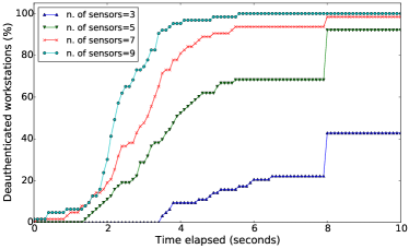
Figure 9: Proportion of deauthenticated workstations.

Figure 10: Percentage of times adversaries can perform an attack on a target workstation, for an increasing number of sensors.

Figure 10 shows the number of opportunities that adversaries have to access the target workstation without being witnessed by the victim, for Insider and Co-worker, respectively. For Insider we consider that he can reach the workstation after 4 seconds since the victim left the office (this a realistic estimate of the time required to walk to the workstation from outside the office). For Co-worker, we consider that he can reach the workstation as soon as the victim user left the office. We consider that every time a user leaves his workstation unattended, an attack is possible. As shown in the plot, with an approach with time-out, both adversaries can perform an attack every time a user leaves the office (63 times in our experiment). Increasing the number of sensors, the attack opportunities significantly decrease, down to zero for 8 or more sensors.

VII-D Usability

To simulate the keyboard and mouse input at the workstations, we refer to the work of Mikkelsen et al [17], where they monitored the keyboard and mouse usage of a sample of 1211 office workplace users. In their analysis, they discretized time in 5 seconds intervals, and found that, on average, users are using the keyboard or the mouse during 78% of these intervals. We refer to their findings, and we simulate the user inputs in each 5 seconds intervals, such that users have a 78% probability of using the mouse or keyboard during an interval.

We assign a cost (as defined in Section VI-A) of $3$ seconds for deactivating a screen saver (some users just remove it before its expiration), and a cost of 13 seconds to re-perform the authentication (this is on average the time users need to correctly input their login information [22]). Moreover, we assume that when a user leaves the proximity of his workstation, all the other users are inside the room and they are using their own workstation (this is a worst case assumption, since some of them might not be in the office and therefore not be impacted by the system decisions).

For the simulation we follow the procedure described in Section VII-C, plus we randomly draw the users keyboard and mouse input distribution over the monitored period. Since the outcome of the system is dependent on the user inputs, we draw this distribution for 100 times to account for possible differences, and average the result.

Table IV shows the total cost for different number of sensors, computed by multiplying the average number of screen savers and deauthentications for their respective cost (i.e, 3 and 13 seconds, respectively). Values between parenthesis show the standard deviation over the 100 runs of the simulation. The results show that while the number of deauthentication decreases with more sensors, due to the improved precision of RE, the number of screen savers does not decrease. This happens because with more sensors we have an higher recall for MD, and therefore the system needs to deal with an increased number of variation windows, and activates more screen savers. However, Table IV shows that the total cost each day is never higher than 37 seconds. This means that on average, one user (we have three users in total) is required to invest ${\sim}13$ seconds each day to collaborate with the system, which is a very acceptable time.

n. of sensors	# screen savers per day	# deauthentication per day	cost (seconds) per day
3	4.272 (0.82)	0.712 (0.36)	22.07
4	8.238 (1.02)	0.926 (0.43)	36.75
5	8.336 (1.09)	0.754 (0.38)	34.81
6	8.414 (1.17)	0.558 (0.29)	32.5
7	8.188 (1.03)	0.136 (0.15)	26.33
8	8.956 (1.22)	0.086 (0.12)	27.99
9	9.094 (1.15)	0.036 (0.09)	27.75

TABLE IV: Number of times the system takes an incorrect decision, and total cost in seconds, for a 8h period.

VIII Conclusions

Current research on authentication mechanism focuses more on the authentication part, and does not thoroughly take into account the importance of the deauthentication procedure. Even if authentication solutions that provide automatic deauthentication exist, they have limitations: they require the user to carry additional devices, they lack realistic threat models, or they require expensive hardware. In this work, we proposed a solution for the deauthentication – FADEWICH – that leverages physical properties of wireless signal propagation, in order to secure unattended workstations in the office workplace. FADEWICH uses the information provided by wireless sensors placed inside the office to learn the behavior of the radio environment, and deauthenticate users when they leave the vicinity of their workstations. In order to evaluate the security and usability of our system, we designed an experiment with very few assumptions, and we carried it out in one office. We showed that, even in a small office where the radio environment is dynamic and busy, our system grants good performance. In particular, when the sensors grant a sufficient coverage of the area inside the office, the system becomes very accurate and fast in the deauthentication (adversaries cannot exploit any opportunity to perform an attack), without disregarding the usability.

VIII-A Discussion and Future Work

The research question behind this paper, was to understand if it was possible to detect and learn the changes in the wireless propagation caused by the movement of users. However, characterizing the behavior of wireless signals in such dynamic, small and cluttered environments has proved to be challenging. Even if the physical phenomena that regulate the propagation of radio signals are known, we could not use them directly to model the environment in our case. In order to obtain an effective system, we had to rely on high level observations on the monitored signal strengths, use machine learning for the classification, and combine these information with the user inputs at the workstation. Even if this is a poor modeling of the movement of users, we realized that in a system with such weak and loose assumptions (e.g., busy wireless channel, multiple users offices, cheap wireless sensors with simple hardware), our results are noteworthy.

In the future, in order to prove that the system can be effective in different environments, we plan to investigate the performance of the system in different setups (other offices, with different dimensions and users). We also want to evaluate its performance considering different placements of the sensors, to understand if the wireless devices currently present in a common office (e.g., desktop computers, Internet of Things devices) are sufficient to obtain valuable results. Furthermore, we also want to explore whether more fine grained information that can be provided by the wireless channel (such as channel state information) can improve the system performance.

-B Feature Analysis

To understand the role of the features of the samples for RE, we study the correlations between them, and their importance in the classification, using all of the nine sensors. Figure 11 shows the correlation between the variances of all the streams, computed over the labeled samples (for brevity, we did not include the entropies and the autocorrelations). In the figure, the label $d_{i}-d_{j}$ identifies the variance of the stream that goes from device $i$ to device $j$. As shown, when the devices are close to each other, their variance reacts in similar ways to the alteration caused by the user who is moving.

Figure 11: Correlations between the variances of streams in the collected samples.

In order to measure the importance of the features, we remove highly correlated and uncorrelated features, and we compute their relative mutual information (RMI) with the class [9]. RMI is a measure of how good the feature is for discriminating between samples that belong to different classes. For a feature whose distribution is $x$, RMI is computed as the percentage difference between the marginal entropy of the feature distribution $H(x)$ and its conditional entropy given the class label $H(x|y)$, with respect to the initial entropy $H(x)$, that is:

$$RMI(x,y)=\frac{H(x)-H(x|y)}{H(x)}.$$

For the quantization, we use 256 linearly distributed bins among the minimum and the maximum of the distribution.

With the RMI values, we plot an heatmap of the importances of the single streams between devices, reported in Figure 12. In the figure, darker areas correspond to stronger importance for the features of the streams that pass through that area, in terms of RMI. As shown, certain devices (e.g., $d_{5}$) do not significantly contribute to the classification, as the their information is either not discriminative, or is strongly correlated with other devices (and is therefore not colored in Figure 12).

Figure 12: Importance of the streams in terms of RMI visualized as an heatmap on the planimetry of the office used for the experiment.

In Table V, we report the 15 features that scored higher in terms of RMI in our data in. The feature names indicate the stream, and the type of feature for that stream, either entropy (ent), variance (var), or autocorrelation (ac).

Rank	feature	RMI
1	d9-d2-ent	0.2977
2	d7-d8-ac	0.2863
3	d7-d1-ent	0.2858
4	d1-d3-ac	0.2809
5	d4-d2-ac	0.2807
6	d3-d5-ac	0.2778
7	d6-d8-ac	0.2776
8	d3-d9-ac	0.2770
9	d6-d2-ac	0.2765
10	d4-d1-ac	0.2761
11	d2-d3-ac	0.2757
12	d1-d9-ac	0.2752
13	d1-d6-var	0.2711
14	d8-d9-ac	0.2707
15	d8-d4-ac	0.2698

TABLE V: RMI for the top 15 ranking features.

-C Comparison

In order to evaluate the usability and security aspects side by side, we introduce a broader indicator for the security, that is the amount of time workstations spend in a vulnerable state (i.e., unattended and authenticated). In fact, in our approach, we are reducing the time that workstations spend in a vulnerable state, while increasing the cost for the users. Figure 13 shows such a trade-off, comparing the time-out approach (with $T=300$ seconds time-out) with the outcome of the system with increasing number of sensors. As shown in the figure, with a time-out approach there is no cost for the users, meanwhile, increasing the number of sensors, the cost increases as well (system is querying users and possibly committing errors in the deauthentication). However, although the cost for the users initially increases, it stabilizes soon for an increasing number of sensors (after four sensors in our experiment). Furthermore, the increment in cost is compensated by an exponential decrement in the vulnerable time. This means that increasing the number of sensors does not add significant burden for the users, while it brings valuable improvements in terms of security.

Figure 13: Comparison between the vulnerable time for the workstations and the total cost for the users, for an approach with time-out, and increasing number of sensors.

References

- [1] A. Al Abdulwahid, N. Clarke, I. Stengel, S. Furnell and C. Reich “A Survey of Continuous and Transparent Multibiometric Authentication Systems” In Conference on Cyber Warfare and Security (ECCWS), 2015
- [2] P. Bahl and V. N. Padmanabhan “RADAR: An in-building RF-based user location and tracking system” In IEEE Conference on Computer Communications (INFOCOM), 2000
- [3] S. P. Banerjee and D. L. Woodard “Biometric Authentication and Identification Using Keystroke Dynamics: A Survey” In Journal of Pattern Recognition Research 7.1, 2012
- [4] M. Bocca, O. Kaltiokallio, N. Patwari and S. Venkatasubramanian “Multiple Target Tracking with RF Sensor Networks” In IEEE Transactions on Mobile Computing (TMC) 13.8, 2014
- [5] J. Bonneau “The Science of Guessing: Analyzing an Anonymized Corpus of 70 Million Passwords” In IEEE Symposium on Security and Privacy (S&P), 2012
- [6] J. Bonneau, C. Herley, P. C. Van Oorschot and F. Stajano “The Quest to Replace Passwords: A Framework for Comparative Evaluation of Web Authentication Schemes” In IEEE Symposium on Security and Privacy (S&P), 2012
- [7] CERT Insider Threat Center “U.S. State of Cybercrime Survey” [Online; accessed 19-July-2016], http://resources.sei.cmu.edu/library/asset-view.cfm?assetid=298318, 2014
- [8] M. D. Corner and B. D. Noble “Zero-Interaction Authentication” In ACM Conference on Mobile Computing and Networking (MobiCom), 2002
- [9] T. M. Cover and J. A. Thomas “Entropy, Relative Entropy and Mutual Information” In Elements of Information Theory, 1991
- [10] S. Eberz, K. B. Rasmussen, V. Lenders and I. Martinovic “Preventing Lunchtime Attacks: Fighting Insider Threats With Eye Movement Biometrics” In Symposium on Network and Distributed System Security (NDSS), 2015
- [11] M. Frank, R. Biedert, E. Ma, I. Martinovic and D. Song “Touchalytics: On the Applicability of Touchscreen Input as a Behavioral Biometric for Continuous Authentication” In IEEE Transactions on Information Forensics and Security 8.1, 2013
- [12] C. Herley and P. Van Oorschot “A Research Agenda Acknowledging the Persistence of Passwords” In IEEE Symposium on Security and Privacy (S&P), 2012
- [13] O. Huhta, P. Shrestha, S. Udar, M. Juuti, N. Saxena and N. Asokan “Pitfalls in Designing Zero-Effort Deauthentication: Opportunistic Human Observation Attacks” preprint, http://arxiv.org/abs/1505.05779 In arXiv, 2015
- [14] O. Kaltiokallio and M. Bocca “Real-Time Intrusion Detection and Tracking in Indoor Environment through Distributed RSSI Processing” In IEEE Real-Time and Embedded Technology and Applications Symposium (RTCSA), 2011
- [15] A. E. Kosba, A. Saeed and M. Youssef “Rasid: A Robust Wlan Device-Free Passive Motion Detection System” In IEEE Conference on Pervasive Computing and Communications (PERCOM), 2012
- [16] S. Mare, A. M. Markham, C. Cornelius, R. Peterson and D. Kotz “ZEBRA: Zero-Effort Bilateral Recurring Authentication” In IEEE Symposium on Security and Privacy (S&P), 2014
- [17] S. Mikkelsen, I. Vilstrup, C. F. Lassen, A. I. Kryger, F. J. Thomsen and J. H. Andersen “Validity of Questionnaire Self-Reports on Computer, Mouse and Keyboard Usage During a Four-Week Period” In Occupational and Environmental Medicine 64.8, 2007
- [18] S. Nouwt, B. R De Vries and C. Prins “Reasonable Wxpectations of Privacy?: Eleven Country Reports on Camera Surveillance and Workplace Privacy” Cambridge University Press, 2005
- [19] N. Patwari and J. Wilson “A Fade-Level Skew-Laplace Signal Strength Model for Device-Free Localization with Wireless Networks” In IEEE Transactions on Mobile Computing (TMC) 11.6, 2012
- [20] C. Pöpper, N. O. Tippenhauer, B. Danev and S. Capkun “Investigation of signal and message manipulations on the wireless channel” In European Conference on Research in Computer Security (ESORICS), 2011
- [21] K. B. Rasmussen, M. Roeschlin, I. Martinovic and G. Tsudik “Authentication Using Pulse-Response Biometrics” In Symposium on Network and Distributed System Security (NDSS), 2014
- [22] R. Shay, L. F. Cranor, S. Komanduri, A. L. Durity, P. S. Huh, M. L. Mazurek, S. M. Segreti, B. Ur, L. Bauer and N. Christin “Can long passwords be secure and usable?” In ACM Conference on Human Factors in Computing Systems (CHI), 2014
- [23] S. Sinclair and S. W. Smith “Access Control Realities As Observed in a Clinical Medical Setting” [Online; accessed 19-July-2016], http://www.cs.dartmouth.edu/reports/TR2012-714.pdf, 2012
- [24] S. Sinclair and S. W. Smith “Preventative Directions For Insider Threat Mitigation Via Access Control” In Insider Attack and Cyber Security, 2008, pp. 165–194
- [25] I. Sluganovic, M. Roeschlin, K. B. Rasmussen and I. Martinovic “Using Reflexive Eye Movements for Fast Challenge-Response Authentication” In ACM Conference on Computer and Communications Security (CCS), 2016
- [26] Software Engineering Institute, Carnegie Mellon University “Insider Threat Study: Illicit Cyber Activity Involving Fraud in the U.S. Financial Services Sector” [Online; accessed 19-July-2016], https://resources.sei.cmu.edu/asset_files/SpecialReport/2012_003_001_28137.pdf, 2012
- [27] Frank Stajano “Pico: No more passwords!” In International Workshop on Security Protocols, 2011, pp. 49–81
- [28] C. M. Tey, P. Gupta and D. Gao “I Can Be You: Questioning the Use of Keystroke Dynamics as Biometrics.” In Symposium on Network and Distributed System Security (NDSS), 2013
- [29] N. O. Tippenhauer, K. B. Rasmussen, C. Pöpper and S. Čapkun “Attacks on Public WLAN-based Positioning Systems” In Conference on Mobile Systems, Applications, and Services (MobiSys), 2009
- [30] B. Ur, F. Noma, J. Bees, S. M. Segreti, R. Shay, L. Bauer, N. Christin and L. F. Cranor ““I Added’!’at the End to Make It Secure”: Observing Password Creation in the Lab” In Symposium On Usable Privacy and Security (SOUPS), 2015
- [31] Verizon “Data Breach Investigation Report” [Online; accessed 19-July-2016], http://www.verizonenterprise.com/verizon-insights-lab/dbir/2016/, 2016
- [32] J. Wilson and N. Patwari “Radio Tomographic Imaging with Wireless Networks” In IEEE Transactions on Mobile Computing (TMC) 9.5, 2010
- [33] Y. Zhao, N. Patwari, J. M. Phillips and S. Venkatasubramanian “Radio Tomographic Imaging and Tracking of Stationary and Moving People via Kernel Distance” In ACM Conference on Information Processing in Sensor Networks (IPSN), 2013