Driven translocation of a semi-flexible polymer through a nanopore

Abstract

We study the driven translocation of a semi-flexible polymer through a nanopore by means of a modified version of the iso-flux tension propagation theory (IFTP), and extensive molecular dynamics (MD) simulations. We show that in contrast to fully flexible chains, for semi-flexible polymers with a finite persistence length $\tilde{\ell}_{p}$ the trans side friction must be explicitly taken into account to properly describe the translocation process. In addition, the scaling of the end-to-end distance $R_{N}$ as a function of the chain length $N$ must be known. To this end, we first derive a semi-analytic scaling form for $R_{N}$, which reproduces the limits of a rod, an ideal chain, and an excluded volume chain in the appropriate limits. We then quantitatively characterize the nature of the trans side friction based on MD simulations of semi-flexible chains. Augmented with these two factors, the modified IFTP theory shows that there are three main regimes for the scaling of the average translocation time $\tau\propto N^{\alpha}$. In the stiff chain (rod) limit $N/\tilde{\ell}_{p}\ll 1$, $\alpha=2$, which continuously crosses over in the regime $1<N/\tilde{\ell}_{p}<4$ towards the ideal chain behavior with $\alpha=3/2$, which is reached in the regime $N/\tilde{\ell}_{p}\sim 10^{2}$. Finally, in the limit $N/\tilde{\ell}_{p}\gg 10^{6}$ the translocation exponent approaches its asymptotic value $1+\nu$, where $\nu$ is the Flory exponent. Our results are in good agreement with available simulations and experimental data.

Introduction – Since the seminal works by Bezrukov et al. Parsegian in 1994, and two years later by Kasianowicz et al. Kasianowicz , polymer translocation through nanopores has become one of the most active research topics in soft condensed matter physics Muthukumar_book ; Milchev_JPCM ; Tapio_Review . It plays an important role in many biological processes such as virus injection and protein transportation through membrane channels Alberts . It also has many technological applications such as drug delivery Meller_JPhysCondMatt , gene therapy and rapid DNA sequencing Kasianowicz ; Meller_PRL_2001 ; Aksimentiev_NanoLett_2008 ; Tapio_PRL_2008 ; Golestanian_PRX_2012 , and has been motivation for many experimental and theoretical studies Tapio_Review ; storm2005 ; branton2008 ; Spencer2014 ; Stein2014 ; sung1996 ; muthu1999 ; metzler2003 ; kantor2004 ; grosberg2006 ; sakaue2007 ; luo2008 ; luo2009 ; schadt2010 ; Milchev_JPCM ; rowghanian2011 ; Muthukumar_book ; bhatta2009 ; dubbeldam2012 ; sakaue2010 ; saito2012a ; ikonen2012a ; ikonen2012b ; jalal2014 ; jalal2015 ; ikonen2013 ; slater2008a ; slater2008b ; Lam_JStatPhys2015 ; dubbeldam2014 ; AniketJCP2013 ; AniketPolymerSciSerC2013 ; ClementiPRL2006 ; DaiPolymers2016 ; NetzEPL2006 .

Most analytical and theoretical studies to date have focused on field-driven translocation of flexible polymers through nanopores. A break-through in this problem came from Sakaue, who employed the idea of tension propagation (TP) to explain the physical mechanism of the driven translocation process sakaue2007 . According to TP theory when the external driving force, which is due to an external electric field across the pore, acts on the bead(s) at the pore in the direction of cis to trans side (see Fig. ​1), a tension front propagates along the backbone of the chain in the cis side of the chain. Consequently, the cis side is divided into mobile and immobile parts, where the mobile part of the chain has been already influenced by the tension force and moves towards the pore, and the immobile part of the chain is in its equilibrium state, i.e. its average velocity is zero.

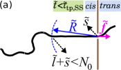
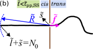
Figure 1: (a) A schematic of the translocation process in the tension propagation (TP) stage, i.e. $\tilde{t}<\tilde{t}_{\textrm{tp,SS}}$, for the strong stretching (SS) regime. $N_{0}$ is the contour length of polymer and the translocation coordinate $\tilde{s}$ equals the number of beads that have already been translocated into the trans side. The number of beads influenced by the tension force is $\tilde{l}+\tilde{s}$, which during TP stage is less than $N_{0}$. $\tilde{R}$ determines the location of the tension front. (b) The translocation process for SS regime during the post propagation stage where the tension front has reached the chain end, which yields $\tilde{l}+\tilde{s}=N_{0}$.

Following Sakaue’s work, in a series of papers Ikonen et al. developed a Brownian dynamics - TP theory (BDTP) to take into account the effect of pore friction, finite chain length, and thermal fluctuations due to the solvent during the course of translocation ikonen2012a ; ikonen2012b . Most recently, the BDTP theory was reformulated within the constant monomer iso-flux approximation rowghanian2011 (IFTP) jalal2014 ; jalal2015 , leading to a fully quantitative and self-consistent theory of dynamics of driven translocation with only one free parameter, the effective pore friction. A key role in the theory is played by the total effective friction, which comprises the constant pore friction (interaction of the monomers with the nanopore) and drag from the cis part of the chain. For fully flexible chains, the contribution from the trans side of the friction can be included in the pore friction, and need not be explicitly considered.

However, in many cases of practical interest the translocating polymers are not fully flexible – e.g. for double-stranded DNA, the persistence length $\ell_{p}$ is typically about 500 Å. To unravel the influence of stiffness to translocation, in this Letter we consider the pore-driven translocation dynamics of semi-flexible polymers with a finite persistence length within the IFTP theory. We argue that unlike for fully flexible chains, the trans side friction has a significant contribution to the dynamics and must be explicitly added to the expression for the total friction. To calculate the chain drag, we derive a semi-analytic form for the end-to-end scaling form $R_{N}$ for semi-flexible chains, which correctly incorporates the various scaling regimes and crossover between them for different ratios of the persistence and chain lengths $\tilde{\ell}_{p}/N$. Neither of these factors have been considered in the previous works AniketJCP2013 ; AniketPolymerSciSerC2013 ; ClementiPRL2006 ; DaiPolymers2016 . When properly augmented with the correct end-to-end scaling form and time-dependent trans side friction, the IFTP theory shows that the average translocation time displays complex scaling and crossover behavior as a function of $\ell_{p}/N$. In the appropriate limits, the IFTP theory also recovers the exactly known results for the scaling exponent of the translocation time. It is important to note that in the IFTP theory there is only one unknown parameter, the effective pore friction $\eta_{\textrm{p}}$, which can be obtained either experimentally or from MD simulations ikonen2012a ; ikonen2012b ; jalal2014 ; jalal2015 .

Theory: (a) Strong stretching regime – In the IFTP theory, we use dimensionless units denoted by tilde as $\tilde{X}\equiv X/X_{u}$, with the units of length $s_{u}\equiv\sigma$, time $t_{u}\equiv\eta\sigma^{2}/(k_{B}T)$, force $f_{u}\equiv k_{B}T/\sigma$, velocity $v_{u}\equiv\sigma/t_{u}=k_{B}T/(\eta\sigma)$, friction $\Gamma_{u}\equiv\eta$, and monomer flux $\phi_{u}\equiv k_{B}T/(\eta\sigma^{2})$, where $\sigma$ is the segment length, $T$ is the temperature of the system, $k_{B}$ is the Boltzmann constant, and $\eta$ is the solvent friction per monomer. The quantities without the tilde, such as the force, friction and length, are expressed in Lennard-Jones units. In the overdamped Brownian limit ikonen2012a ; ikonen2012b ; jalal2014 ; jalal2015 , the equation of motion for the translocation coordinate $\tilde{s}$ which is the number of beads in the trans side (see Fig. ​1), is given by

$$\tilde{\Gamma}(\tilde{t})\frac{d\tilde{s}}{d\tilde{t}}=\tilde{f}+\tilde{\zeta}(\tilde{t})\equiv\tilde{f}_{\textrm{tot}},$$ (1)

where $\tilde{\Gamma}(\tilde{t})$ is the effective friction, and $\tilde{\zeta}(\tilde{t})$ is Gaussian white noise which satisfies $\langle\zeta(t)\rangle=0$ and $\langle\zeta(t)\zeta(t^{\prime})\rangle=2\Gamma(t)k_{B}T\delta(t-t^{\prime})$, $\tilde{f}$ is the external driving force, and $\tilde{f}_{\textrm{tot}}$ is the total force.

In the iso-flux assumption the monomers flux, $\tilde{\phi}\equiv d\tilde{s}/d\tilde{t}$, on the mobile domain in the cis side and also through the pore is constant in space, but evolves in time rowghanian2011 ; jalal2014 . The tension front, which is the boundary between the mobile and immobile domains, is located at distance $\tilde{x}=-\tilde{R}(\tilde{t})$ from the pore. The external driving force acts on the monomer(s) inside the pore located at $\tilde{x}=0$ (see Fig. ​1(a)).

It has been shown ikonen2012a ; ikonen2012b ; jalal2014 ; jalal2015 ; ikonen2013 that for flexible polymers the friction can be written as $\tilde{\Gamma}(\tilde{t})=\tilde{\eta}_{\rm cis}(\tilde{t})+\tilde{\eta}_{\textrm{p}}$, and the translocation dynamics is essentially controlled by the time-dependent friction $\tilde{\eta}_{\rm cis}(\tilde{t})$ on the cis side of the chain, whereas the trans side friction is negligible and can be absorbed into the constant pore friction $\tilde{\eta}_{\textrm{p}}$. In the case of semi-flexible chains this approximation is not justified. Within the IFTP theory, the friction due to the trans side of the chain $\tilde{\eta}_{\rm TS}$ can be taken into account as follows. In the strong stretching (SS) regime of strong driving, where the mobile part of the chain in the cis side is fully straightened (cf. Figs. ​1(a) and (b)), we can integrate the force balance equation over the mobile domain jalal2014 and the monomer flux becomes

$$\tilde{\phi}(\tilde{t})=\frac{\tilde{f}_{\textrm{tot}}(\tilde{t})}{\tilde{R}(\tilde{t})+\tilde{\eta}_{\textrm{p}}+\tilde{\eta}_{{}_{\textrm{TS}}}}.$$ (2)

By combining Eqs. ​(1) and (2), the effective friction is obtained as

$$\tilde{\Gamma}(\tilde{t})=\tilde{R}(\tilde{t})+\tilde{\eta}_{\textrm{p}}+\tilde{\eta}_{{}_{\textrm{TS}}}.$$ (3)

The time evolution of $\tilde{s}$ is determined by Eqs. (1), (2) and (3), but knowledge of the position of the tension front on the cis side of the chain $\tilde{R}(\tilde{t})$ is still required to find the full solution. We will derive the equation of motion for $\tilde{R}(\tilde{t})$ separately for the TP and post propagation (PP) stages. In the TP stage the tension has not be reached the chain end as presented in Fig. 1 ​(a), while in the PP stage the final monomer has been already influenced by the tension force (see Fig. 1 ​(b)).

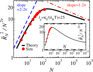
Figure 2: Normalized end-to-end distance $\tilde{R}_{N}^{2}/N^{2\nu}$ as a function of the contour length of the polymer $N$ for fixed value of bending rigidity (in the MD simulations) $\kappa_{{b}}=30$, which corresponds to $\ell_{p}=25$, when $k_{B}T=1.2$. The black curve shows the analytical formula of Eq. ​(4) while red dots present the MD simulations results. Inset shows crossover from Gaussian to self-avoiding behavior for an extended range of $N$.

(b) End-to-end distance of a semi-flexible chain – To find the equation of motion for $\tilde{R}(\tilde{t})$, which is the root-mean-square of the end-to-end distance, an analytical form of $\tilde{R}(\tilde{t})$ for semi-flexible chains is needed. To this end, we have carried out extensive MD simulations of bead-spring models of semi-flexible chains in 3D. The technical details can be found in the Supplementary Material (SM). The MD simulations have been done for different values of contour length $N\sigma$ and bending rigidity $\kappa_{{b}}$. In 3D the persistence length $\ell_{{p}}$ can be expressed as a function of $\kappa_{{b}}$ as $\ell_{{p}}=\kappa_{{b}}/(k_{B}T)$. We find that the MD data (cf. Fig. ​2) is well described for all values of $N/\tilde{\ell}_{{p}}$ by the following semi-empirical analytic expression for the end-to-end distance of a semi-flexible chain:

$$\tilde{R}_{N}=\bigg{\{} \tilde{R}^{2}_{F}-\frac{\tilde{R}^{4}_{F}}{2a_{1}N^{2}}\bigg{[}1-\exp\bigg{(}-\frac{2a_{1}N^{2}}{\tilde{R}^{2}_{F}}\bigg{)}\bigg{]}$$ (4)

$$+2\tilde{\ell}_{{p}}N\!-\frac{2\tilde{\ell}_{{p}}^{2}}{b_{1}}\bigg{[}1\!-\!\exp\bigg{(}\!\!-\frac{b_{1}N}{\tilde{\ell}_{{p}}}\bigg{)}\!\bigg{]}\!\bigg{\}}^{\frac{1}{2}}.$$

Here $\tilde{R}_{F}=A\tilde{\ell}_{{p}}^{\nu_{{p}}}N^{\nu}$, with $\nu_{{p}}=1/(d+2)$ ($d=3$) which describes the scaling of the chain in the limit $N/\tilde{\ell}_{p}\gg 1$ Nakanishi and is correctly recovered by Eq. ​(4). In the opposite stiff or rod-like chain limit of $N/\tilde{\ell}_{{p}}\ll 1$, Eq. ​(4) recovers the trivial result that $\tilde{R}_{N}=N$. The quantity $\nu=0.588$ is the Flory exponent, and $A=0.8$, $a_{1}=0.1$ and $b_{1}=0.9$ are constants. In the intermediate regime $4\lesssim N/\tilde{\ell}_{{p}}\lesssim 400$ which here corresponds to $10^{2}\lesssim N\lesssim 10^{4}$ for $\tilde{\ell}_{{p}}=25$, a crossover occurs from a rod-like chain to a Gaussian (ideal) polymer, followed by an eventual crossover to a self-avoiding chain for $N/\tilde{\ell}_{{p}}\gg 10^{6}$ Hsu as can be seen in the inset of Fig. ​2. Remarkably, we find that Eq. ​(4) is universally valid with the same values of $A,a_{1}$ and $b_{1}$ for a wide range of values of $\tilde{\ell}_{p}$, as shown in SM. It should be noted that the amplitude $A$ is fixed by the equilibrium scaling of the chain, and thus only $a_{1}$ and $b_{1}$ are fitting parameters.

(c) Time evolution of the tension front – Using $\tilde{R}(\tilde{t})$ in Eq. ​(4) together with the mass conservation $N=\tilde{l}+\tilde{s}$, where $\tilde{l}=\tilde{R}$, the equation of motion for the tension front in the TP stage for the SS regime (see Fig. ​1(a)) can be derived as

$$\dot{\tilde{R}}(\tilde{t})\!=\!\frac{\tilde{\phi}(\tilde{t})~{}(\cal{G}+\cal{H})}{2\tilde{R}(\tilde{t})-(\cal{G}+\cal{H})},$$ (5)

where

$${\cal{G}} = \!\!\frac{\tilde{R}^{2}_{F}}{N}\bigg{[}2\nu-(2-2\nu)~{}\exp\bigg{(}-\frac{2a_{1}N^{2}}{\tilde{R}^{2}_{F}}\bigg{)}\bigg{]}$$

$$+ \frac{(4\nu-2)\tilde{R}^{4}_{F}}{2a_{1}N^{3}}\bigg{[}-1+\exp\bigg{(}-\frac{2a_{1}N^{2}}{\tilde{R}^{2}_{F}}\bigg{)}\bigg{]},$$

$${\cal{H}} = 2~{}\tilde{\ell}_{{p}}\bigg{[}1-\exp\bigg{(}-\frac{b_{1}N}{\tilde{\ell}_{{p}}}\bigg{)}\bigg{]}.$$ (6)

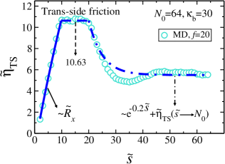
Figure 3: The trans side friction $\tilde{\eta}_{{}_{\textrm{TS}}}(\tilde{s})$ as a function of $\tilde{s}$ for fixed values of the chain length $N_{0}=64$, bending rigidity $\kappa_{\textrm{b}}=30$, and external driving force $f=20$. The turquoise circles are MD data. The blue solid, dashed and dashed-dotted lines represent the three different regimes (see the text and SM for details).

In the PP stage (see Fig. 1(b)) the correct closure relation is $\tilde{l}+\tilde{s}=N_{0}$. Then one can derive the equation of motion for the tension front in PP stage as

$$\dot{\tilde{R}}(\tilde{t})=-\tilde{\phi}(\tilde{t}).$$ (7)

To find the solution, in the TP stage, Eqs. ​(1), (2), (3) and (5) must be solved self-consistently while in the PP stage, Eqs. ​(1), (2), (3), (7) must be solved.

Results: (a) Trans side friction – We present the waiting time distribution $w(\tilde{s})$, which is the time that each bead spends at the pore, in SM. The data clearly show that in order to have a quantitative theory, we must include $\tilde{\eta}_{\rm TS}(t)$ in Eq. ​(3).

It is expected that the trans side friction is a complicated function of the driving force, chain length and the bending rigidity, and the present IFTP theory does not allow us to derive it analytically. To this end, we have extracted it numerically from the MD simulations as shown in Fig. ​3. Details and additional data for smaller driving forces and for different persistence lengths are in SM. We can identify three distinct regimes in $\tilde{\eta}_{\rm TS}(\tilde{s})$. For small $\tilde{s}/N_{0}$, we find that the friction grows proportional to the $x$ component of the end-to-end distance $\tilde{R}_{x}$. After this initial stage it saturates to a constant value (here $\approx 10.63$), which from the MD simulations indicates buckling of the trans part of the chain. This buckling of the chain reduces the friction and we find an approximately exponential decay of the friction towards an asymptotic constant $\tilde{\eta}_{\rm TS}(N_{0})\approx 5.5$.

(b) Translocation time exponent – The scaling of the average translocation time as a function of the chain length $\tau\propto N_{0}^{\alpha}$ is a fundamental characteristic of translocation dynamics. For flexible chains it scales as $\tau=a_{p}N_{0}+a_{c}N_{0}^{\nu+1}$, where $a_{p}$ and $a_{c}$ are constants. The first term is due to the pore friction which causes a significant finite-size correction to the asymptotic scaling where $\alpha={\nu+1}$ ikonen2012a ; ikonen2012b ; ikonen2013 ; jalal2014 ; jalal2015 . The asymptotics is, of course, recovered for the semi-flexible chains in the large $N_{0}$ limit when $\tilde{\ell}_{p}/N_{0}\ll 1$. On the other hand, in the limit of a rod-like polymer $\tau\propto N_{0}^{2}$. Following Ref. ​jalal2014 , we can derive an analytic expression for $\tau$ by assuming that only the external driving force $\tilde{f}$ contributes to the total force in the BD equation (1). This leads to reduction of Eq. ​(2) to $\tilde{\phi}(\tilde{t})=\tilde{f}/\big{[}\tilde{R}(\tilde{t})+\tilde{\eta}_{\textrm{p}}+\tilde{\eta}_{{}_{\textrm{TS}}}\big{]}$, and the total translocation time can be written as

$$\tilde{\tau}=\frac{1}{\tilde{f}}\bigg{[}\int_{0}^{N_{0}}\tilde{R}_{N}dN+\tilde{\eta}_{\textrm{p}}N_{0}\bigg{]}+\tilde{\tau}_{\textrm{TS}},$$ (8)

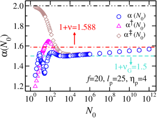
Figure 4: The effective translocation time exponents as a function of the chain length $N_{0}$ for $\ell_{{p}}=25$ and pore friction $\eta_{\textrm{p}}=4$, and external driving force $f=20$. The blue circles show the translocation exponent $\alpha$ as a function of $N_{0}$, while pink triangles and brown diamonds show the rescaled translocation exponents $\alpha^{{\dagger}}$ and $\alpha^{{\ddagger}}$, respectively. The horizontal black dashed-dotted-dotted, red dashed-dotted and turquoise dashed lines show the asymptotic rod-like, excluded volume chain and Gaussian scaling limits, respectively. See text for details.

where $\tilde{\tau}_{\textrm{TS}}=\big{[}\int_{0}^{N_{0}}\tilde{\eta}_{{}_{\textrm{TS}}}dN+\int_{0}^{\tilde{R}_{N_{0}}}(\tilde{\eta}_{{}_{\textrm{TS,pp}}}-\tilde{\eta}_{{}_{\textrm{TS,tp}}})d\tilde{R}\big{]}/\tilde{f}$ is the trans side contribution to the translocation time. The second term in $\tilde{\tau}_{TS}$ is due to non-monotonic behavior of $\tilde{\eta}_{\textrm{TS}}$ in the TP and PP stages. In the rod limit we obtain the simple analytical result that

$$\tilde{\tau}=\frac{1}{\tilde{f}}\bigg{[}\tilde{\eta}_{{p}}N_{0}+N_{0}^{2}\bigg{]},$$ (9)

which gives the asymptotic exponent $\alpha=2$. The corresponding effective exponents will be between unity and two.

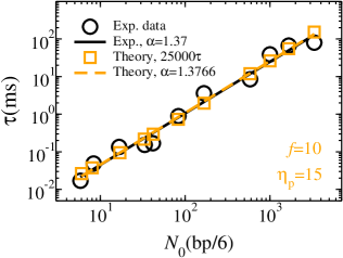
Figure 5: Translocation time $\tau$ as a function of the chain length $N_{0}$. Black circles are experimental data in Fig. ​6(c) of Ref. ​Spencer2014 while orange squares are data from the IFTP theory, where we have used the coarse grained model. Each bead contains 6 bps. The value of the external driving force in the IFTP theory is $f=10$ and the pore friction is $\eta_{\textrm{p}}=15$. The translocation time for the IFTP theory has been multiplied by a factor of 25000 to agree with the experimental time scale. The black solid and orange dashed lines are linear fitting curves to experimental and IFTP theory, respectively. Similar results can be obtained for the values of the external driving forces $f=5$ and $20$. Details on mapping the experimental data to theory are explained in Sec. ​I of SM.

To quantify the influence of the trans side and pore friction on the effective translocation exponent we define two rescaled translocation exponents $\alpha^{{\dagger}}$ and $\alpha^{{\ddagger}}$ as $\tau^{{\dagger}}=\tau-\tau_{\textrm{TS}}\sim N_{0}^{\alpha^{{\dagger}}}$ and $\tau^{{\ddagger}}=\tau-\tau_{\textrm{TS}}-a_{\textrm{p}}N_{0}\sim N_{0}^{\alpha^{{\ddagger}}}$, respectively. In the short ($N_{0}/\tilde{\ell}_{{p}}\lesssim 4$) and intermediate ($4\lesssim N_{0}/\tilde{\ell}_{{p}}\lesssim 400$) chain limits, contributions from both the trans side and pore friction are important as can be seen in Eq. ​(8).

In Fig. ​4 we show the detailed dependence of the effective translocation time exponents as a function of the chain length $N_{0}$ for constant values of the persistence length $\ell_{{p}}=25$, pore friction $\eta_{\textrm{p}}=4$ and driving force $f=20$. The blue circles show the effective value of the total $\alpha$ as a function of $N_{0}$. The non-monotonic behavior of the trans side friction leads into a non-monotonic dependence of $\alpha$ on $N_{0}$. Interestingly enough, there is an extended intermediate range of chain lengths where the exponent is very close to the Gaussian value $\alpha=3/2$ and slowly approaches its asymptotic value of $1+\nu=1.588$ from below. We note that in order to see this crossover it is necessary to have a full scaling form for the end-to-end distance of the form of Eq. ​(4).

To quantify how the trans side friction affects the effective translocation exponent, in Fig. ​4 we plot $\alpha^{{\dagger}}$ (pink triangles). It approaches $\alpha$ for $N_{0}>10^{4}$, where the trans side friction becomes negligible. Finally, the rescaled translocation exponent $\alpha^{{\ddagger}}$ (brown diamonds), which is the effective translocation time exponent in the absence of both trans side and pore friction, is also plotted as a function of $N_{0}$. This exponent recovers the rod-like limit for very short chains. It merges with the other two effective exponents to the almost Gaussian value at intermediate lengths and eventually approaches $\nu+1$, as expected.

Finally, we compare the results of IFTP theory with relevant experiments. In Fig. ​5, we present the translocation time obtained from experiments (black circles) and from the augmented IFTP theory (orange squares) as a function of the chain length $N_{0}({\textrm{bp}}/6)$, for fixed values of external driving force $f=10$ and pore friction $\eta_{\textrm{p}}=15$. The value of external driving force $f=10$ corresponds to potential difference $V=200$ mV across the pore in the experiments Spencer2014 (for more information see SM.) To match the length scales, we coarse grain such that one bead in our model contains 6 bps. With this choice the translocation exponent from the IFTP theory (orange dashed line) is in good agreement with the exponent from the experimental data (black solid line).

Summary and Conclusions – We have shown here that in addition to the case of fully flexible polymers, the IFTP theory provides the proper theoretical framework for driven translocation of semi-flexible polymers. The two key quantities required are an explicit determination of the trans side friction and a proper analytical formula for the end-to-end distance of semi-flexible polymers. The augmented IFTP theory can quantitatively describe all the relevant scaling regimes for the scaling exponent of the average translocation time, and crossover between them. It also reproduces the exactly known limits and is in good agreement with available experimental data.

Acknowledgments – J.S. thanks V. Thakore, H.-P. Hsu and R.R. Netz for enlightening discussions. This work was supported by the Academy of Finland through its Centers of Excellence Program under Project Nos. 251748 and 284621. The numerical calculations were performed using computer resources from the Aalto University School of Science “Science-IT” project, and from CSC - Center for Scientific Computing Ltd. This research was funded in part by the National Institutes of Health (R01-HG009186, M.W.).

References

- (1) S. M. Bezrukov, I. Vodyanoy and A. V. Parsegian, Nature 370, 279 (1994).
- (2) J. J. Kasianowicz, E. Brandin, D. Branton and D. W. Deamer, Proc. Natl. Acad. Sci. USA 93, 13770 (1996).
- (3) M. Muthukumar, Polymer Translocation (Taylor and Francis, 2011).
- (4) A. Milchev, J. Phys.: Condens. Matter 23, 103101 (2011).
- (5) V. V. Palyulin, T. Ala-Nissila and R. Metzler, Soft Matter 10, 9016 (2014).
- (6) B. Alberts, A. Johnson, J. Lewis, M. Raff, K. Roberts and P. Walter, Molecular Biology of the Cell (Garland Science, 2002).
- (7) A. Meller, J. Phys.: Condens. Matter, 15 R581 (2003).
- (8) A. Meller, L. Nivon and D. Branton, Phys. Rev. Lett. 86 3435 (2001).
- (9) G. Sigalov, J. Comer, G. Timp and A. Aksimentiev, Nano Lett. 8, 56 (2008).
- (10) K. Luo, T. Ala-Nissila, S.-C. Ying and A. Bhattacharya, Phys. Rev. Lett. 100, 058101 (2008).
- (11) J. A. Cohen, A. Chaudhuri. and R. Golestanian, Phys. Rev. X 2, 021002 (2012).
- (12) A. J. Storm et al, Nano Lett. 5, 1193 (2005).
- (13) D. Branton, D. W. Deamer, A. Marziali et al., Nature Biotech. 26, 1146 (2008).
- (14) S. Carson, J. Wilson, A. Aksimentiev and M. Wanunu, Biophys. J. 107, 2381 (2014).
- (15) A. McMullen, H. W. de Haan, J. X. Tang and D. Stein, Nat. Comms. 5, 4171 (2014).
- (16) W. Sung and P. J. Park, Phys. Rev. Lett. 77, 783 (1996).
- (17) M. Muthukumar, J. Chem. Phys. 111, 10371 (1999).
- (18) R. Metzler and J. Klafter, Biophys. J. 85, 2776 (2003).
- (19) Y. Kantor and M. Kardar, Phys. Rev. E 69, 021806 (2004).
- (20) A. Y. Grosberg, S. Nechaev, M. Tamm and O. Vasilyev, Phys. Rev. Lett. 96, 228105 (2006).
- (21) T. Sakaue, Phys. Rev. E 76, 021803 (2007).
- (22) K. Luo, S. T. T. Ollila, I. Huopaniemi, T. Ala-Nissila, P. Pomorski, M. Karttunen, S.-C. Ying and A. Bhattacharya, Phys. Rev. E 78 050901(R) (2008).
- (23) K. Luo, T. Ala-Nissila, S.-C. Ying and R. Metzler, Europhys. Lett. 88, 68006 (2009).
- (24) E. Schadt, S. Turner and A. Kasarskis, Hum. Mol. Gen. 19, R227 (2010).
- (25) P. Rowghanian and A. Y. Grosberg, J. Phys. Chem. B 115, 14127 (2011).
- (26) A. Bhattacharya, W.H. Morrison, K. Luo, T. Ala-Nissila, S.-C. Ying, A. Milchev and K. Binder, Eur. Phys. J. E 29, 423 (2009).
- (27) J. L. A. Dubbeldam, V. G. Rostiashvili, A. Milchev and T. A. Vilgis, Phys. Rev. E 85, 041801 (2012).
- (28) T. Sakaue, Phys. Rev. E 81, 041808 (2010).
- (29) T. Saito and T. Sakaue, Phys. Rev. E 85, 061803 (2012).
- (30) T. Ikonen, A. Bhattacharya, T. Ala-Nissila and W. Sung, Phys. Rev. E 85, 051803 (2012).
- (31) T. Ikonen, A. Bhattacharya, T. Ala-Nissila and W. Sung, J. Chem. Phys. 137, 085101 (2012).
- (32) J. Sarabadani, T. Ikonen and T. Ala-Nissila, J. Chem. Phys. 141, 214907 (2014).
- (33) J. Sarabadani, T. Ikonen and T. Ala-Nissila, J. Chem. Phys. 143, 074905 (2015).
- (34) T. Ikonen, A. Bhattacharya, T. Ala-Nissila, W. Sung, Europhys. Lett 103, 38001 (2013).
- (35) M. G. Gauthier and G. W. Slater, J. Chem. Phys. 128, 065103 (2008).
- (36) M. G. Gauthier and G. W. Slater, J. Chem. Phys. 128, 205103 (2008).
- (37) P.M. Lam and Y. Zhen, J. Stat. Phys. 161, 197 (2015). It should be noted that this reference does not recover the correct translocation exponents for the limits of a rod, a Gaussian and a self-avoiding chain.
- (38) J. L. A. Dubbeldam, V. G. Rostiashvili and T. A. Vilgis, J. Chem. Phys. 141, 124112 (2014).
- (39) R. Adhikari and A. Bhattacharya, J. Chem. Phys. 138, 204909 (2013).
- (40) A. Bhattacharya, Polym. Sci. Ser. C 55, 60 (2013).
- (41) S. Matysiak, A. Montesi, M. Pasquali, A. B. Kolomeisky and C. Clementi, Phys. Rev. Lett. 96, 118103 (2006).
- (42) Z.-Y. Yang, A.-H. Chai, Y.-F. Yang, X.-M. Li, P. Li and R.-Y. Dai, Polymers 8, 332 (2016).
- (43) X. Schlagberger, J. Bayer, J. O. Rädler and R. R. Netz, Europhys. Lett. 76 (2), 346 (2006).
- (44) H. Nakanishi, J. Physique 48, 979 (1987).
- (45) H.-P. Hsu, W. Paul and K. Binder, Macromol. Theory and Simulations 20, 510 (2011).