Thinner is not Always Better: Cascade Knapsack Problems

Abstract

In the context of branch-and-bound (B&B) for integer programming (IP) problems, a direction along which the polyhedron of the IP has minimum width is termed a thin direction. We demonstrate that a thin direction need not always be a good direction to branch on for solving the problem efficiently. Further, the integer width, which is the number of B&B nodes created when branching on the direction, may also not be an accurate indicator of good branching directions.

Keywords: Branch-and-bound; hyperplane branching; thin direction; column basis reduction.

1 Introduction

Deciding which variables, or combinations of variables, to branch on is perhaps the most critical step that determines the performance of any branch-and-bound (B&B) algorithm to solve integer programs (IPs); see [5], for instance. Most state of the art IP and mixed integer programming (MIP) solvers use branching on individual variables (rather than their combinations). Variable selection done by the default B&B branching on individual variables can be viewed as a special case of selecting hyperplanes in the more general B&B that branches on linear combinations of variables. Branching on hyperplanes is one of the key steps in Lenstra’s seminal algorithm for solving integer programs (IPs) in fixed dimensions [15]. This theoretical algorithm finds a sequence of “thin” directions, i.e., directions along which the width of the polyhedron of the IP is “small”. Branching on these thin directions in sequential order will solve the IP relatively quickly. The thin directions are identified using lattice basis reduction.

When individual binary variables are present, the default choice to branch on them (as opposed to finding good combinations of the variables) is in line with the idea of selecting thin directions. Recall that a binary variable $x_{j}$ satisfies $0\leq x_{j}\leq 1$, and hence the width of the polyhedron along the direction of $x_{j}$ is not larger than $1$. Motivated in part by the use of thin directions in Lenstra’s algorithm, the author and Pataki previously created and analyzed [13] a general class of inequality-constrained knapsack feasibility problems called decomposable knapsack problems (DKPs), whose coefficients have the form $\mathbf{a}=\mathbf{p}M+\mathbf{r}$ for a suitably large positive number $M$. We showed that DKPs are difficult for ordinary branch-and-bound, i.e., B&B branching on individual variables (an independent analysis of the difficulty of B&B on integer knapsacks was presented separately [12]). At the same time, $\mathbf{p}$ indicates a thin direction for the DKPs, and hence the problems are easy when one branches on the backbone hyperplane defined by $\mathbf{p}\mathbf{x}$. The DKPs subsume several known families of hard IPs, including those proposed by Jeroslow [9], Todd as well as Avis (as attributed to by Chvátal) [6], and by Aardal and Lenstra [3]. All these instances suggest that branching on thin directions—as represented by individual binary variables in typical instances, or by the backbone constraint given by $\mathbf{p}\mathbf{x}$ in the case of DKPs—is typically a good choice for B&B algorithms.

Even when such thin directions are present in an IP instance, identifying them might not be straightforward. We had previously proposed [13] a simple preconditioning method termed column basis reduction (CBR) that provides reformulations of general IPs. For the DKPs, we proved that the thin direction $\mathbf{p}\mathbf{x}$ is identified as the last variable in the preconditioned IP given by CBR. Branching on the last variable solves the problem in one step.

Our Contribution:

We demonstrate that branching on thin directions need not always lead to B&B algorithms running efficiently. On the other hand, branching on certain directions that are not thin might lead to quick convergence of B&B algorithms on certain instances. To this end, we create a generalization of the DKPs called cascade knapsack problems (CKPs), which are inequality-constrained binary knapsack feasibility problems whose coefficients have the form $\mathbf{a}=\mathbf{p}_{1}M_{1}+\mathbf{p}_{2}M_{2}+\mathbf{r}$. We show that the width of CKP polytope along $\mathbf{p}_{1}$ is larger than $1$, while the width along unit directions is equal to $1$. As such, $\mathbf{p}_{1}$ is not a thin direction. Similarly, $\mathbf{p}_{2}$ is also not a thin direction. Nonetheless, branching on the hyperplane defined by $\mathbf{p}_{1}\mathbf{x}$ followed by branching on the hyperplane defined by $\mathbf{p}_{2}\mathbf{x}$ solves the problem quickly, while the original CKP is hard for ordinary B&B. A similar behavior is observed even when we consider integer width, which is the number of nodes created when branching on a hyperplane, in place of width. We also show that this behavior extends to higher order CKPs, e.g., with $\mathbf{a}=\mathbf{p}_{1}M_{1}+\mathbf{p}_{2}M_{2}+\mathbf{p}_{3}M_{3}+\mathbf{r}$.

We demonstrate that column basis reduction (CBR) is effective in solving the CKPs quickly in practice. Extending the previous analysis for DKPs [13], we argue that branching on the collection of good directions defined by $\mathbf{p}_{1}\mathbf{x},\mathbf{p}_{2}\mathbf{x},\mathbf{p}_{3}\mathbf{x},\dots$ is captured by branching on the last few variables in the preconditioned IP give by CBR.

1.1 Related Work

Following Lenstra’s algorithm [15], Kannan [10], and Lovász and Scarf [17] developed similar algorithms for solving IPs in fixed dimension. Cook et al. [7] reported a practical implementation of the algorithm of Lovász and Scarf [17], and obtained reductions in the number of nodes in the B&B tree for solving certain network design problems. At the same time, finding the branching direction(s) at each node was quite expensive.

Mahajan and Ralphs [18] showed that it is NP-hard to find branching directions that are optimal with respect to width. On the other hand, Aardal and co-workers studied a basis reduction-based reformulation technique for equality constrained IPs, which uses the idea of branching on good hyperplanes [1, 2, 3]. Specifically, Aardal and Lenstra [3] studied a class of equality-constrained integer knapsack problems whose reformulations have a specific thin direction, which is also identified by a reformulation technique. Our preconditioning method CBR [13] applies to more general, i.e., not necessarily equality-constrained, IPs. The reformulation technique of Aardal et al. is subsumed by the more general CBR.

The use of branching on good hyperplanes on more general IPs was demonstrated by Aardal et al. [1], who used their basis reduction-based reformulation technique to solve otherwise hard-to-solve marketshare problems, which are multiple equality-constrained binary IPs [8, 11]. Louveaux and Wolsey [16] extended these results to a more general class of IPs with some special structure. In related work, Mehrotra and Li [19] proposed a general framework for identifying branching hyperplanes for mixed IPs, which also benefits from basis reduction.

Pataki, Tural, and Wong [20] studied the efficacy of branch-and-bound on CBR-type reformulations of general IPs. In particular, they proved an upper bound on the width of the polyhedron of the reformulated IP along the last unit vector. This bound implies that as the size of coefficients in the constraint matrix of the original IP increases, the reformulation of almost all instances generated from a standard distribution is solved at the root node. This result follows from the fact that the last unit vector in the reformulation is equivalent to a direction along which the width of the original polyhedron is small, and hence branching on the last unit vector solves the problems easily.

2 Width, Integer Width, and Branching Directions: Examples

Definition 2.1.

Given a polyhedron $Q$, and an integer vector $\mathbf{c}$, the width and the integer width of $Q$ in the direction of $\mathbf{c}$ are

$$0pt(\mathbf{c},Q) =~{}\max\{\mathbf{c}\mathbf{x}\,|\,\mathbf{x}\in Q\}-\min\{\mathbf{c}\mathbf{x}\,|\,\mathbf{x}\in Q\,\},$$

$${\rm iwidth}(\mathbf{c},Q) =~{}\lfloor\max\{\mathbf{c}\mathbf{x}\,|\,\mathbf{x}\in Q\}\rfloor-\lceil\min\{\mathbf{c}\mathbf{x}\,|\,\mathbf{x}\in Q\}\rceil+1.$$

Further, an integer direction $\mathbf{c}^{*}$ is termed a thin direction of $Q$ if $~{}\displaystyle\mathbf{c}^{*}\in~{}\operatorname{argmin}\limits_{\mathbf{c}}\,0pt(\mathbf{c},Q)$. The quantity ${\rm iwidth}(\mathbf{c},Q)\,$ is the number of nodes generated by branch-and-bound when branching on the constraint given by $\mathbf{c}\mathbf{x}$.

We point out that integer width is not given by requiring the optima in the definition of width be attained by integer vectors. Consider the simple 2D example where $Q=\{\mathbf{x}\in{\mathbb{R}}^{2}\,|\,0\leq x_{1},x_{2}\leq 1\}$. For $\mathbf{c}=\begin{bmatrix}1&0\end{bmatrix}$, we get that $0pt(\mathbf{c},Q)=1$, with the maximum and minimum being attained by $\mathbf{x}=\begin{bmatrix}1&0\end{bmatrix}$ and the zero vector, respectively. But ${\rm iwidth}(\mathbf{c},Q)=2$, since we would consider two branches when branching on the direction defined by $x_{1}$, corresponding to $x_{1}=1$ and $x_{1}=0$.

We present several instances of integer programming which demonstrate that thin directions might not always be the best choices for branching. On the contrary, certain specific directions along which the width, or even the integer width, of the polytope is larger than the minimum (integer) width could help solve the problem quickly using B&B.

We consider classes of inequality-constrained binary knapsack feasibility problems of the form

$$\{\mathbf{x}\in\mathbb{Z}^{n}~{}|~{}\beta^{\prime}\leq\mathbf{a}\mathbf{x}\leq\beta,~{}\mathbf{0}\leq\mathbf{x}\leq\mathbf{1}\},$$

that have no integer feasible solutions, and our goal is to prove its integer infeasibility using B&B. For an integer program labeled ${\rm(IP)}$ and an integer vector $\mathbf{c}$, we denote by $0pt(\mathbf{c},{\rm IP})$ the width of the LP-relaxation of ${\rm(IP)}$ in the direction $\mathbf{c}$, and similarly denote ${\rm iwidth}(\mathbf{c},{\rm IP})$.

Our use of the term knapsack problem is a generalization of how it is referred to in most literature (see, e.g., [22, Section 16.6]), where the single constraint has the form $\mathbf{a}\mathbf{x}\leq\beta$ (or $\mathbf{a}\mathbf{x}=\beta$ in the equality version). It happens to be the case that we have $\beta^{\prime}=\beta$ in all the following examples (KP1,KP2,KP3,KP4). But our construction (in Section 3) is more general, allowing $\beta^{\prime}<\beta$. Indeed, several of the larger instances we present (see Table 1) do have $\beta^{\prime}<\beta$.

Example 2.2.

Consider the following knapsack feasibility problem with $n=12$ binary variables:

$$\begin{array}[]{rcl}75\,x_{1}+~{}86\,x_{2}+~{}97\,x_{3}+~{}105\,x_{4}+~{}142\,x_{5}+~{}153\,x_{6}~{}+\\ 161\,x_{7}+172\,x_{8}+209\,x_{9}+217\,x_{10}+228\,x_{11}+239\,x_{12}{}&=&1023\\ 0\leq\,x_{j}\,\leq 1,~{}~{}x_{j}\in\,{\mathbb{Z}},~{}~{}j=1,\dots,12.\end{array}$$ (KP1)

There are no integer feasible solutions, and CPLEX 12.6.3.0 applying branch-and-cut on the original variables without using any objective function takes $484$ B&B nodes to prove integer infeasibility of this instance (we mention here that all computations presented in this document were done on an Intel PC with $8$ cores and a $2.33$ GHz CPU using CPLEX 12.6.3.0 as the MIP solver). The knapsack coefficient vector $\mathbf{a}=(75,~{}86,\dots,239)$ is a thin direction (trivially), as $0pt(\mathbf{a},\mbox{\ref{kp1}})=0$. It can also be checked that $0pt(\mathbf{e}_{j},\rm{\ref{kp1}})=1$ for all unit vectors $\mathbf{e}_{j}$, as the maximum and minimum of $x_{j}$ over (KP1) are $1$ and $0$, respectively, for all $j\in\{1,\dots,12\}$.

The knapsack coefficients have the form $\mathbf{a}=\mathbf{p}_{1}M_{1}+\mathbf{p}_{2}M_{2}+\mathbf{r}$, where

$$\begin{array}[]{rcccccccccccccc}\mathbf{p}_{1}&=&(\phantom{-}1,&1,&1,&1,&2,&2,&2,&2,&3,&3,&3,&3),&\\ \mathbf{p}_{2}&=&(\phantom{-}1,&2,&3,&4,&1,&2,&3,&4,&1,&2,&3,&4),&\mbox{and}\\ \mathbf{r}&=&(-1,&0,&1,&-1,&0,&1,&-1,&0,&1,&-1,&0,&1).\end{array}$$ (1)

$0pt(\mathbf{p}_{1},\rm{\ref{kp1}})=13.99-12.13=1.86$, which is larger than the width along any $\mathbf{e}_{j}$. Still, we branch on the direction of $\mathbf{p}_{1}$ by adding the constraint $\,\mathbf{p}_{1}\mathbf{x}=13$. We now get the maximum and minimum of $\mathbf{p}_{2}\mathbf{x}$ for this branch as $16.90$ and $16.10$. Thus, branching on the hyperplanes defined by $\mathbf{p}_{1}\mathbf{x}$ and $\mathbf{p}_{2}\mathbf{x}$ in that order proves the integer infeasibility of the instance easily, in only two B&B nodes. We also point out that $0pt(\mathbf{p}_{2},\rm{\ref{kp1}})=22.16-9.99=12.17$, and hence does not define a helpful direction to branch on.

One could argue that while $0pt(\mathbf{p}_{1},\ref{kp1})$ is indeed larger than the width along any individual variable, ${\rm iwidth}(\mathbf{p}_{1},\ref{kp1})=1$ is in fact smaller than ${\rm iwidth}(\mathbf{e}_{j},\ref{kp1})=1-0+1=2$. But the next two examples illustrate that small integer widths might also not indicate good branching directions.

Example 2.3.

Consider the following knapsack feasibility problem with $n=12$ binary variables:

$$\begin{array}[]{rcl}71\,x_{1}+~{}\,82\,x_{2}+~{}93\,x_{3}+~{}101\,x_{4}+134\,x_{5}+145\,x_{6}~{}~{}~{}~{}+\\ 153\,x_{7}+164\,x_{8}+197\,x_{9}+205\,x_{10}+216\,x_{11}+227\,x_{12}{}{}&=&981\\ 0\leq\,x_{j}\,\leq 1,~{}~{}x_{j}\in\,{\mathbb{Z}},~{}~{}j=1,\dots,12.\\ \end{array}$$ (KP2)

There are no integer feasible solutions, and CPLEX 12.6.3.0 applying branch-and-cut on the original variables without using any objective function takes $462$ B&B nodes to prove integer infeasibility of this instance. Similar to (KP1), we get $0pt(\mathbf{a},\ref{kp2})=0$ and $0pt(\mathbf{e}_{j},\ref{kp2})=1$ for all unit vectors $\mathbf{e}_{j}$.

The knapsack coefficient vector $\mathbf{a}=(71,~{}82,\dots,227)$ has the same structure as in (KP1), using the same vectors $\mathbf{p}_{1},\mathbf{p}_{2},\mathbf{r}$ in Equation (1), except with $M_{1}=62$. We observe that $0pt(\mathbf{p}_{1},$ $\ref{kp2})=14.17-12.22=1.95$ and ${\rm iwidth}(\mathbf{p}_{1},\ref{kp2})=2$, which is equal to the integer width along each $\mathbf{e}_{j}$. Nonetheless, branching on the hyperplane defined by $\mathbf{p}_{1}\mathbf{x}$ followed by that defined by $\mathbf{p}_{2}\mathbf{x}$ solves the problem in only three B&B nodes, as shown in Figure 1. Similar to (KP1), $0pt(\mathbf{p}_{2},\rm{\ref{kp2}})=22.25-10.23=12.02$, and hence $\mathbf{p}_{2}\mathbf{x}$ does not define a good direction to branch on.

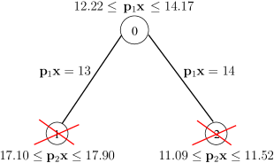
Figure 1: Branching tree for (KP2). Crossed out nodes are pruned due to integer infeasibility.

Example 2.4.

Consider the following knapsack feasibility problem with $n=12$ binary variables:

$$\begin{array}[]{rcl}57\,x_{1}+68\,x_{2}+~{}79\,x_{3}+~{}87\,x_{4}+~{}106\,x_{5}+~{}117\,x_{6}~{}~{}~{}~{}+\\ 125\,x_{7}+136\,x_{8}+155\,x_{9}+163\,x_{10}+174\,x_{11}+185\,x_{12}{}&=&847\\ 0\leq\,x_{j}\,\leq 1,~{}~{}x_{j}\in\,{\mathbb{Z}},~{}~{}j=1,\dots,12.\\ \end{array}$$ (KP3)

There are no integer feasible solutions, and CPLEX 12.6.3.0 applying branch-and-cut on the original variables without using any objective function takes $451$ B&B nodes to prove integer infeasibility of this instance. Similar to (KP1) and (KP2), we get $0pt(\mathbf{a},\ref{kp3})=0$ and $0pt(\mathbf{e}_{j},$ $\ref{kp3})=1$ for all unit vectors $\mathbf{e}_{j}$.

The knapsack coefficient vector $\mathbf{a}=(57,~{}68,\dots,185)$ has the same structure as in (KP1), using the same vectors $\mathbf{p}_{1},\mathbf{p}_{2},\mathbf{r}$ in Equation (1), except with $M_{1}=48$. We observe that $0pt(\mathbf{p}_{1},$ $\ref{kp3})=15.22-12.86=2.36$ and ${\rm iwidth}(\mathbf{p}_{1},\ref{kp3})=3$, which is strictly greater than the integer width along each $\mathbf{e}_{j}$. Nonetheless, branching on the hyperplane defined by $\mathbf{p}_{1}\mathbf{x}$ followed by that defined by $\mathbf{p}_{2}\mathbf{x}$ solves the problem in only four B&B nodes, as shown in Figure 2. Similar to (KP1) and (KP2), $0pt(\mathbf{p}_{2},\rm{\ref{kp3}})=22.90-11.62=11.28$, and $\mathbf{p}_{2}\mathbf{x}$ does not define a good direction to branch on.

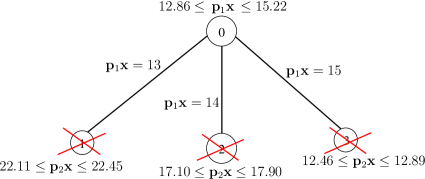
Figure 2: Branching tree for (KP3). Crossed out nodes are pruned due to integer infeasibility.

These three examples have a common property: the effect of branching on the hyperplane defined by $\mathbf{p}_{1}\mathbf{x}$ cascades down to the subproblems created in this process, which are all pruned by branching subsequently on the hyperplane defined by $\mathbf{p}_{2}\mathbf{x}$. Hence we call them cascade knapsack problems (CKPs). The next example illustrates that the cascading effect could be observed over multiple $\mathbf{p}_{i}\mathbf{x}$ directions, i.e., branching on the hyperplane defined by $\mathbf{p}_{1}\mathbf{x}$ cascades down, and then the effect of branching on the hyperplane defined by $\mathbf{p}_{2}\mathbf{x}$ cascades down to the next levels of nodes, followed by branching on the hyperplane defined by $\mathbf{p}_{3}\mathbf{x}$, and so on.

Example 2.5.

Consider the following knapsack feasibility problem with $n=12$ binary variables:

$$\begin{array}[]{rcl}723\,x_{1}+~{}799\,x_{2}+~{}875\,x_{3}~{}+~{}981\,x_{4}~{}+~{}1285\,x_{5}+~{}1361\,x_{6}~{}~{}~{}+\\ 1467\,x_{7}+1587\,x_{8}+1847\,x_{9}+1953\,x_{10}+2029\,x_{11}+2116\,x_{12}{}{}&=&9312\\ 0\leq\,x_{j}\,\leq 1,~{}~{}x_{j}\in\,{\mathbb{Z}},~{}~{}j=1,\dots,12.\\ \end{array}$$ (KP4)

The knapsack coefficients have the form $\,\mathbf{a}=\mathbf{p}_{1}M_{1}+\mathbf{p}_{2}M_{2}+\mathbf{p}_{3}M_{3}+\mathbf{r}\,$ for the same set of vectors $\mathbf{p}_{1},\mathbf{p}_{2},$ and $\mathbf{r}$ given in Equation (1), with $\mathbf{p}_{3}=(\,5,~{}3,~{}1,~{}2,~{}4,~{}2,~{}3,~{}5,~{}3,~{}4,~{}2,~{}1\,)$, and $M_{1}=572,M_{2}=97$, and $M_{3}=11$. The vector $\mathbf{p}_{3}$ is chosen to be linearly independent of $\mathbf{p}_{1}$ and $\mathbf{p}_{2}$ here. This knapsack problem is also integer infeasible, and CPLEX 12.6.3.0 branching on the original variables takes $491$ B&B nodes to prove integer infeasibility. Further, $0pt(\mathbf{a},\ref{kp4})=0$ and $0pt(\mathbf{e}_{j},\ref{kp4})=1$ for all $j$, as in the previous instances. At the same time, we can solve this problem easily if we branch on the hyperplanes defined by $\mathbf{p}_{1}\mathbf{x},\mathbf{p}_{2}\mathbf{x},$ and $\mathbf{p}_{3}\mathbf{x}$, in that order. The branching tree is shown in Figure 3, and the problem is solved in seven B&B nodes.

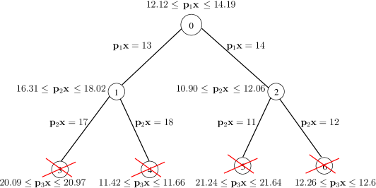
Figure 3: Branching tree for (KP4). Crossed out nodes are pruned due to integer infeasibility.

We could present a similar instance with $\,\mathbf{a}=\mathbf{p}_{1}M_{1}+\mathbf{p}_{2}M_{2}+\mathbf{p}_{3}M_{3}+\mathbf{r}\,$ where the integer width of its LP relaxation along $\mathbf{p}_{1}$ is $3$, similar to (KP3). Just as in (KP4), we solve this problem quickly if we branch on the hyperplanes defined by $\mathbf{p}_{1}\mathbf{x},\mathbf{p}_{2}\mathbf{x},$ and $\mathbf{p}_{3}\mathbf{x}$, in that order.

3 Procedure for creating a CKP

We present a procedure (Figure 4) to create CKP instances with the structure illustrated in Example 2.2 (KP1), where $\mathbf{a}=\mathbf{p}_{1}M_{1}+\mathbf{p}_{2}M_{2}+\mathbf{r}$ and branching on the hyperplane defined by $\mathbf{p}_{1}\mathbf{x}$ followed by branching on the hyperplane defined by $\mathbf{p}_{2}\mathbf{x}$ solves the problem easily. The remaining examples (KP2, KP3, KP4) as well as the instances reported in Section 4 were generated by appropriate modifications of this procedure. We use the following notation in the description.

Definition 3.1.

For $x\in{\mathbb{R}}$, we define

$$\downharpoonright\!x\!\downharpoonleft=\left\{\begin{array}[]{c@{\mbox{ if }}l}\lfloor x\rfloor&x\not\in{\mathbb{Z}},\\ x-1&x\in{\mathbb{Z}};\end{array}\right.~{}~{}~{}\mbox{and}~{}~{}~{}\upharpoonright\!x\!\upharpoonleft=\left\{\begin{array}[]{c@{\mbox{ if }}l}\lceil x\rceil&x\not\in{\mathbb{Z}},\\ x+1&x\in{\mathbb{Z}}.\end{array}\right.$$

Other notation:

We denote the vector of ones by $\mathbf{1}$, and the box with upper bound $\mathbf{1}$ by $B_{\mathbf{1}}=\{\,\mathbf{x}\in{\mathbb{R}}^{n}\,|\,\mathbf{0}\leq\mathbf{x}\leq\mathbf{1}\}$. We denote by $\mathbb{Z}^{n}_{+}$ the set of all $n$-vectors with positive integer entries.

Procedure CKP Input: Vectors $\mathbf{p}_{1},\mathbf{p}_{2},\mathbf{r}$ with $\mathbf{p}_{1},\mathbf{p}_{2}\in\mathbb{Z}^{n}_{+}$, $\mathbf{r}\in\mathbb{Z}^{n}$, and $\mathbf{p}_{1},\mathbf{p}_{2}$ linearly independent. Output: $M_{1},M_{2},\beta^{\prime},\beta$ forming the CKP instance with $\mathbf{a}=\mathbf{p}_{1}M_{1}+\mathbf{p}_{2}M_{2}+\mathbf{r}$. 1. Choice of $k_{1},k_{2}$: $$\begin{array}[]{c}\mbox{Find}~{}\gamma_{1}=\max\{\mathbf{p}_{1}\mathbf{x}\,|\,\mathbf{x}\in B_{\mathbf{1}}\},~{}\delta_{1}=\min\{\mathbf{p}_{1}\mathbf{x}\,|\,\mathbf{x}\in B_{\mathbf{1}}\};~{}\mbox{set}~{}k_{1}=\lfloor\,(\downharpoonright\!\gamma_{1}\!\downharpoonleft+\upharpoonright\!\delta_{1}\!\upharpoonleft)/2\,\rceil.\\ \vspace*{-0.1in}\hfil\\ \mbox{Find }\gamma_{2}=\max\{\mathbf{p}_{2}\mathbf{x}~{}|~{}\mathbf{p}_{1}\mathbf{x}=k_{1}+1,~{}\mathbf{x}\in B_{\mathbf{1}}\},{}\\ \mbox{ and }~{}\,\delta_{2}=\min\,\{\mathbf{p}_{2}\mathbf{x}~{}|~{}\mathbf{p}_{1}\mathbf{x}=k_{1}+1,~{}\mathbf{x}\in B_{\mathbf{1}}\};{}{}\\ ~{}~{}~{}~{}~{}~{}~{}~{}\mbox{set}~{}k_{2}=\lfloor\,(\downharpoonright\!\gamma_{2}\!\downharpoonleft+\upharpoonright\!\delta_{2}\!\upharpoonleft)/2\,\rceil.\end{array}$$ (2) 2. Choice of $M_{2},\beta^{\prime}_{2},\beta_{2}$: $$\begin{array}[]{rcl}\mbox{Find }~{}\eta_{2}&=&\max\{\mathbf{r}\mathbf{x}~{}|~{}\mathbf{p}_{1}\mathbf{x}=k_{1}+1,\mathbf{p}_{2}\mathbf{x}\leq k_{2},~{}\mathbf{x}\in B_{\mathbf{1}}\},\\ ~{}\mbox{ and }\mu_{2}&=&\min\,\{\mathbf{r}\mathbf{x}~{}|~{}\mathbf{p}_{1}\mathbf{x}=k_{1}+1,\mathbf{p}_{2}\mathbf{x}\geq k_{2}+1,~{}\mathbf{x}\in B_{\mathbf{1}}\}.\end{array}$$ (3) $$\mbox{If}~{}\upharpoonright\!\eta_{2}\!\upharpoonleft-\downharpoonright\!\mu_{2}\!\downharpoonleft\geq 1,~{}\mbox{set}~{}M_{2}=\upharpoonright\!\eta_{2}\!\upharpoonleft-\downharpoonright\!\mu_{2}\!\downharpoonleft,~{}\mbox{and set}~{}~{}\mathbf{a}_{2}=\mathbf{p}_{2}M_{2}+\mathbf{r}.$$ (4) $$\begin{array}[]{rcl}\mbox{Find }~{}\eta^{\prime}_{2}&=&\max\,\{\mathbf{a}_{2}\mathbf{x}~{}|~{}\mathbf{p}_{1}\mathbf{x}=k_{1}+1,\,\mathbf{p}_{2}\mathbf{x}\leq k_{2},~{}\mathbf{x}\in B_{\mathbf{1}}\},\\ \vspace*{-0.15in}\hfil\\ \mbox{ and }\mu^{\prime}_{2}&=&\min\,\,\{\mathbf{a}_{2}\mathbf{x}~{}|~{}\mathbf{p}_{1}\mathbf{x}=k_{1}+1,~{}\mathbf{p}_{2}\mathbf{x}\geq k_{2}+1,~{}\mathbf{x}\in B_{\mathbf{1}}\}.\end{array}$$ (5) $$\mbox{If }\upharpoonright\!\eta^{\prime}_{2}\!\upharpoonleft\leq\downharpoonright\!\mu^{\prime}_{2}\!\downharpoonleft~{}~{}\mbox{set}~{}\beta^{\prime}_{2}=\upharpoonright\!\eta^{\prime}_{2}\!\upharpoonleft~{}\mbox{ and }~{}\beta_{2}=\downharpoonright\!\mu^{\prime}_{2}\!\downharpoonleft.$$ (6) 3. Choice of $M_{1},\beta^{\prime}_{1},\beta_{1},$:   $$\begin{array}[]{c}\mbox{Find }~{}\eta_{1}~{}=~{}\max\,\{\mathbf{a}_{2}\mathbf{x}~{}|~{}\mathbf{p}_{1}\mathbf{x}\leq k_{1},~{}\mathbf{x}\in B_{\mathbf{1}}\},~{}~{}~{}~{}~{}~{}\mbox{ and }{}\\ \mu_{1}~{}=~{}\min\,\,\{\mathbf{a}_{2}\mathbf{x}~{}|~{}\mathbf{p}_{1}\mathbf{x}\geq k_{1}+2,~{}\mathbf{x}\in B_{\mathbf{1}}\}.\end{array}$$ (7) $$\mbox{Set }~{}M_{1}=\upharpoonright\!\max\,(\,\eta_{1}-\beta^{\prime}_{2},\,\beta_{2}-\mu_{1},\,M_{2})\!\upharpoonleft.$$ (8) $$\mbox{Set }~{}\mathbf{a}_{1}=\mathbf{p}_{1}M_{1}+\mathbf{a}_{2},~{}~{}\beta^{\prime}_{1}=\beta^{\prime}_{2}+(k_{1}+1)M_{1},~{}\mbox{ and }~{}\beta_{1}=\beta_{2}+(k_{1}+1)M_{1}.\mbox{\hskip 14.45377pt}$$ (9) 4. Output instance:  Set $\beta^{\prime}=\beta^{\prime}_{1},\,\beta=\beta_{1},\,\mathbf{a}=\mathbf{a}_{1}$, and return $(M_{1},M_{2},\beta^{\prime},\beta,\mathbf{a})$.

Figure 4: Procedure to generate CKPs.

We now present two lemmas describing the Procedure (Figure 4). Notice that we refer to both the final knapsack problem and its LP relaxation as (CKP), with the exact choice evident from the context.

Lemma 3.2.

If the quantities defined in Equations (4), (6), and (8) exist, then (CKP)$\wedge\,(\mathbf{p}_{1}\mathbf{x}=k_{1}+1)\,\neq\,\emptyset$.

Proof.

Let $\mathbf{x}_{1}$ and $\mathbf{x}_{2}$ attain the optima for the LPs in Equation (7) (the maximum and the minimum, respectively), based on which $M_{1}$ is defined in Equation (8). We get

$$\max\{\mathbf{a}_{1}\mathbf{x}~{}|~{}\mathbf{p}_{1}\mathbf{x}\leq k_{1},\mathbf{x}\in B_{\mathbf{1}}\} \leq k_{1}M_{1}+\max\{\mathbf{a}_{2}\mathbf{x}~{}|~{}\mathbf{p}_{1}\mathbf{x}\leq k_{1},\mathbf{x}\in B_{\mathbf{1}}\}=k_{1}M_{1}+\eta_{1}$$

$$= [(k_{1}+1)M_{1}+\beta^{\prime}_{2}]-\,(M_{1}-(\eta_{1}-\beta^{\prime}_{2}))$$

$$= \beta^{\prime}_{1}-\,(M_{1}-(\eta_{1}-\beta^{\prime}_{2}))$$

$$< \beta^{\prime}_{1}.$$

The third equality follows from the definition of $\beta^{\prime}_{1}$ in Equation (9), and the last strict inequality follows from the definition of $M_{1}$ in Equation (8). Similarly, we get

$$\min\{\mathbf{a}_{1}\mathbf{x}~{}|~{}\mathbf{p}_{1}\mathbf{x}\geq k_{1}+2,\mathbf{x}\in B_{\mathbf{1}}\} \geq (k_{1}+2)M_{1}+\min\{\mathbf{a}_{2}\mathbf{x}~{}|~{}\mathbf{p}_{1}\mathbf{x}\geq k_{1}+2,\mathbf{x}\in B_{\mathbf{1}}\}$$

$$= (k_{1}+2)M_{1}+\mu_{1}$$

$$= [(k_{1}+1)M_{1}+\beta_{2}]+\,(M_{1}-(\beta_{2}-\mu_{1}))$$

$$= \beta_{1}+\,(M_{1}-(\beta_{2}-\mu_{1}))$$

$$> \beta_{1}.$$

Hence $\mathbf{x}^{\prime}\in\{\mathbf{x}~{}|~{}\beta^{\prime}_{1}\leq\mathbf{a}_{1}\mathbf{x}\leq\beta_{1},\,\mathbf{x}\in B_{\mathbf{1}}\}\,$ implies that $\,k_{1}<\mathbf{p}_{1}\mathbf{x}^{\prime}<k_{1}+2$. Further, since $\mathbf{a}_{2}$ and $\mathbf{p}_{1}$ have positive entries, the structure of the LPs in Equation (7) implies that we will have $\mathbf{p}_{1}\mathbf{x}_{1}=k_{1}$ and $\mathbf{p}_{1}\mathbf{x}_{2}=k_{1}+2$. Thus we can find a constant $\lambda\in(0,1)$ such that $\mathbf{x}^{\prime}=\lambda\mathbf{x}_{1}+(1-\lambda)\mathbf{x}_{2}\,$ satisfies $\,\beta^{\prime}_{1}\leq\mathbf{a}_{1}\mathbf{x}^{\prime}\leq\beta_{1}$ with $\mathbf{p}_{1}\mathbf{x}^{\prime}=k_{1}+1$. This result implies when we branch on the hyperplane defined by $\mathbf{p}_{1}\mathbf{x}$ in the original (CKP) problem, the branch created by setting $\mathbf{p}_{1}\mathbf{x}=k_{1}+1$ cannot be pruned due to LP infeasibility. ∎

Lemma 3.3.

If the quantities defined in Equations (4), (6), and (8) exist, then the integer infeasibility of (CKP) is proven by $~{}(\mathbf{p}_{1}\mathbf{x}=k_{1}+1)\,\bigwedge\,(\mathbf{p}_{2}\mathbf{x}\leq k_{2}\,\vee\,\mathbf{p}_{2}\mathbf{x}\geq k_{2}+1)$.

Proof.

Let $\mathbf{x}_{3}$ and $\mathbf{x}_{4}$ attain the optima for the LPs in Equation (5) (the maximum and the minimum, respectively). Since $\,\eta^{\prime}_{2}<\beta^{\prime}_{2}\leq\beta_{2}<\mu^{\prime}_{2},\,$ and due to the way $\mathbf{a}_{1},\beta^{\prime}_{1},$ and $\beta_{1}$ are defined (in Equation (9)), there is some $\lambda^{\prime}\in(0,1)$ such that $\mathbf{x}^{\prime\prime}=\lambda^{\prime}\mathbf{x}_{3}+(1-\lambda^{\prime})\mathbf{x}_{4}$ and $\mathbf{x}^{\prime\prime}\in\{\mathbf{x}~{}|~{}\beta^{\prime}_{1}\leq\mathbf{a}_{1}\mathbf{x}\leq\beta_{1},\,\mathbf{p}_{1}\mathbf{x}=k_{1}+1,\,\mathbf{x}\in B_{\mathbf{1}}\}$. Since $\mathbf{a}_{2}$ and $\mathbf{p}_{2}$ both have positive entries, the structure of LPs in Equation (5) implies we have $\mathbf{p}_{2}\mathbf{x}_{3}=k_{2}$ and $\mathbf{p}_{2}\mathbf{x}_{4}=k_{2}+1$. Further,

$$\begin{array}[]{ll}&\mathbf{x}^{\prime\prime}\in\{\mathbf{x}\,|\,\beta^{\prime}_{1}\leq\mathbf{a}_{1}\mathbf{x}\leq\beta_{1},\,\mathbf{p}_{1}\mathbf{x}=k_{1}+1,\,\mathbf{x}\in B_{\mathbf{1}}\}\\ ~{}\Rightarrow&\mathbf{x}^{\prime\prime}\in\{\mathbf{x}\,|\,\beta^{\prime}_{2}\leq\mathbf{a}_{2}\mathbf{x}\leq\beta_{2},\,\mathbf{p}_{1}\mathbf{x}=k_{1}+1,\,\mathbf{x}\in B_{\mathbf{1}}\}\\ ~{}\Rightarrow&k_{2}<\mathbf{p}_{2}\mathbf{x}^{\prime\prime}<k_{2}+1,\end{array}$$

as $\mathbf{x}^{\prime\prime}=\lambda^{\prime}\mathbf{x}_{3}+(1-\lambda^{\prime})\mathbf{x}_{4}$ must hold for some $\lambda^{\prime}\in(0,1)$. Thus (CKP)$\wedge\,(\mathbf{p}_{1}\mathbf{x}=k_{1}+1)\,\neq\,\emptyset$ as already shown by Lemma 3.2, and (CKP)$\wedge~{}(\mathbf{p}_{1}\mathbf{x}=k_{1}+1)\,\bigwedge\,(\mathbf{p}_{2}\mathbf{x}\leq k_{2}\,\vee\,\mathbf{p}_{2}\mathbf{x}\geq k_{2}+1)\,=\,\emptyset$. ∎

The preceding two lemmas show that branching on the hyperplane defined by $\mathbf{p}_{1}\mathbf{x}$ followed by that defined by $\mathbf{p}_{2}\mathbf{x}$ proves the integer infeasibility of (CKP). While Lemma 3.2 shows the existence of some $\mathbf{x}^{\prime}\in$ (CKP) satisfying $\mathbf{p}_{1}\mathbf{x}^{\prime}=k_{1}+1$, we have not explicitly shown that $0pt(\mathbf{p}_{1},{\rm CKP})>1$. In fact, the Procedure (in Figure 4) is not guaranteed to work on every choice of the input vectors. For instance, we might not get a valid choice for $M_{2}$ in Equation (4), or for $\beta^{\prime}$ and $\beta$ in Equation (6). Further, while the Procedure assumes only that $\mathbf{p}_{1}$ and $\mathbf{p}_{2}$ are linearly independent, we might not get the required structure for the CKP if they are “too close to each other”, e.g., when $n$ is large and the two vectors differ in only one or two entries.

To create instances with ${\rm iwidth}(\mathbf{p}_{1},{\rm CKP})=2$ as in (KP2), we could replace the constraint $\mathbf{p}_{1}\mathbf{x}=k_{1}+1$ in Equations (2), (3), and (5) with $~{}k_{1}+1\leq\mathbf{p}_{1}\mathbf{x}\leq k_{1}+2$, and the constraint $\mathbf{p}_{1}\mathbf{x}\geq k_{1}+2$ in Equation (7) with $\mathbf{p}_{1}\mathbf{x}\geq k_{1}+3$. Alternatively, we could make only the latter change (to $\mathbf{p}_{1}\mathbf{x}\geq k_{1}+3$), while sticking with $\mathbf{p}_{1}\mathbf{x}=k_{1}+1$ in the former Equations, as we did in computational tests reported in the following Section.

Example 2.2 continued: We created the instance (KP1) using the procedure described in Figure 4. We obtained $\gamma_{1}=24$ and $\delta_{1}=0$, setting $k_{1}=12$, and then $\gamma_{2}=23,\,\delta_{2}=9$, setting $k_{2}=16$. The remaining parameter values are obtained as follows. $\eta_{2}=4,\,\mu_{2}=-4,$ giving $M_{2}=10$, and $\eta^{\prime}_{2}=164,\,\mu^{\prime}_{2}=166$, and hence $\beta^{\prime}_{2}=\beta_{2}=165$. We finally get $\eta_{1}=221,\,\mu_{1}=100$, giving $M_{1}=66$, and $\beta^{\prime}_{1}=\beta_{1}=1023$.

4 Computational Tests on CKPs

We used a modification of Procedure CKP to generate ten instances of CKP with the structure illustrated by Example 2.5 (KP4), i.e., with $\mathbf{a}_{1}=\mathbf{p}_{1}M_{1}+\mathbf{p}_{2}M_{2}+\mathbf{p}_{3}M_{3}+\mathbf{r}$, for $n=50$. To keep the knapsack coefficients relatively small, the entries of $\mathbf{p}_{1},\mathbf{p}_{2},$ and $\mathbf{p}_{3}$ are chosen randomly from $\{1,2,3\}$ and those of $\mathbf{r}$ from $\{-1,0,1\}$, such that no two $a_{j}$’s are identical. We tried to solve the original formulations of the CKP, the CKP with $\mathbf{p}_{1}\mathbf{x}$ fixed, and the CKP with $\mathbf{p}_{1}\mathbf{x}$ and $\mathbf{p}_{2}\mathbf{x}$ fixed. All calculations are done on an Intel PC with $8$ cores and a $2.33$ GHz CPU. As an MIP solver, we used CPLEX 12.6.3.0. For feasibility versions of integer programs, the sum of the variables is used as the dummy objective function. Ideally, these problems are expected to become easier when $\mathbf{p}_{1}\mathbf{x}$, and then $\mathbf{p}_{2}\mathbf{x}$, are fixed. At the same time, all the subproblems obtained by fixing $\mathbf{p}_{1}\mathbf{x}=k_{1}+1$ and then $\mathbf{p}_{2}\mathbf{x}=k_{2}+1$ still remain relatively hard—they all remain unsolved after one hour of computational time. For the record, the number of B&B nodes examined within this time for all the runs was 41 $\pm$ 12 million (mean $\pm$ std. dev.). The details of the computations are provided in Table 1. Notice that the CKP instances remain relatively hard for ordinary B&B even after branching on both the hyperplanes defined by $\mathbf{p}_{1}\mathbf{x}$ and $\mathbf{p}_{2}\mathbf{x}$.

Table 1: Statistics for CKP instances of size $n=50$ with ${\rm iwidth}(\mathbf{p}_{1}|{\rm CKP})=2$, ${\rm iwidth}(\mathbf{p}_{2}|({\rm CKP})\wedge\mathbf{p}_{1}\mathbf{x}=k_{1}+1)=2$ and ${\rm iwidth}(\mathbf{p}_{3}|({\rm CKP})\wedge\mathbf{p}_{1}\mathbf{x}=k_{1}+1\wedge\mathbf{p}_{2}\mathbf{x}=k_{2}+1)=0$. $a_{\min}$ and $a_{\max}$ give the smallest and largest knapsack coefficients. $w_{i}$ gives $0pt(\mathbf{p}_{i},{\rm CKP})$ for $i=1,2,3$. ${\rm w}_{j1}$ gives $0pt(\mathbf{p}_{j},({\rm CKP})\wedge\mathbf{p}_{1}\mathbf{x}=k_{1}+1)$ for $j=2,3$. ${\rm w}_{312}$ gives $0pt(\,\mathbf{p}_{3},({\rm CKP})\wedge\mathbf{p}_{1}\mathbf{x}=k_{1}+1\,\wedge\,\mathbf{p}_{2}\mathbf{x}=k_{2}+1)$. For each instance, the original CKP, the CKP after fixing $\mathbf{p}_{1}\mathbf{x}=k_{1}+1$, as well as the CKP after fixing both $\mathbf{p}_{1}\mathbf{x}=k_{1}+1$ and $\mathbf{p}_{2}\mathbf{x}=k_{2}+1$ were all unsolved after the one hour time limit. CBR gives the number of B&B nodes examined to solve the CBR-based reformulation, which was integer infeasible for every instance. The times taken to obtain the CBR-reformulation and to solve it were negligible – each step took less than $1$ second.

	CKP numbers				CKP widths						CBR
#	$a_{\min}$	$a_{\max}$	$\beta^{\prime}$	$\beta$	${\rm w}_{1}$	${\rm w}_{2}$	${\rm w}_{3}$	${\rm w}_{21}$	${\rm w}_{31}$	${\rm w}_{312}$	BB
1	13354	26674	424920	424921	2.005	42.02	41.89	2.443	38.92	0.946	7
2	12251	24467	367732	367733	2.073	40.90	43.07	2.421	38.84	0.944	11
3	14456	28877	416513	416514	2.050	42.91	40.35	2.083	37.37	0.944	8
4	14549	28490	461490	461491	2.033	42.95	42.17	2.037	38.57	0.941	2
5	15375	30716	457004	457005	2.007	42.01	41.82	2.011	39.60	0.943	10
6	11234	21946	326617	326618	2.077	38.93	40.86	2.449	39.02	0.943	20
7	11306	22578	336621	336622	2.077	38.97	39.74	2.369	37.73	0.943	16
8	14696	29358	437657	437658	2.054	44.96	41.80	2.161	38.74	0.943	10
9	15722	31407	453190	453191	2.050	44.91	42.20	2.141	37.95	0.947	12
10	15145	30255	466572	466573	2.036	42.95	39.77	2.011	37.61	0.944	14

All these instances of (CKP) are integer infeasible. They have an integer width of $2$ along $\mathbf{p}_{1}$, and for one of the two subproblems created by branching on the hyperplane defined by $\mathbf{p}_{1}\mathbf{x}$, the integer width along $\mathbf{p}_{2}$ is $2$ as well. The other subproblem is not guaranteed to have this property. In four of the instances, the other subproblem is solved by branching on the hyperplane defined by $\mathbf{p}_{2}\mathbf{x}$ (integer width along $\mathbf{p}_{2}$ is zero), while for the remaining six instances, the integer width along $\mathbf{p}_{2}$ is $1$. For all ten instances, the integer infeasibility of the subproblems created by branching on the hyperplane defined by $\mathbf{p}_{2}\mathbf{x}$ (if any) is proven by branching on the hyperplane defined by $\mathbf{p}_{3}\mathbf{x}$ in the next level. As mentioned previously, this modified version of Procedure CKP cannot be guaranteed to work for every choice of problem parameters. Still, we used the modified procedure as a guideline to search for appropriate parameters that generated instances with the desired structure. As part of the computational tests, we tried to solve the original CKP, the original CKP with $\mathbf{p}_{1}\mathbf{x}$ fixed, and also the original CKP with $\mathbf{p}_{1}\mathbf{x}$ and $\mathbf{p}_{2}\mathbf{x}$ fixed.

The instances are available online at http://www.math.wsu.edu/faculty/bkrishna/CKP/.

4.1 Column Basis Reduction and CKPs

We applied the reformulation technique termed column basis reduction (CBR) [13] on the CKP instances. CBR is a simple preconditioning method for IP feasibility that replaces the problem

$$\{\mathbf{x}\in{\mathbb{Z}}^{n}~{}|~{}\mathbf{b}^{\prime}\leq A\,\mathbf{x}\leq\mathbf{b}\}~{}~{}\mbox{ with }~{}~{}\{\mathbf{y}\in{\mathbb{Z}}^{n}~{}|~{}\mathbf{b}^{\prime}\leq AU\,\mathbf{y}\leq\mathbf{b}\},$$ (10)

where $U$ is a unimodular matrix computed using basis reduction (BR) applied on $A$, which makes the columns of $A$ short, i.e., have small euclidean norms, and nearly orthogonal. The variables $\mathbf{y}$ in the reformulation and the original variables $\mathbf{x}$ are related as $\mathbf{y}=U^{-1}\mathbf{x}$. Standard methods of BR include the Lenstra-Lenstra-Lovász (LLL) reduction [14], which runs in time polynomial time, and versions of Korkine-Zolotarev (KZ) reduction including block-KZ or BKZ reduction [21], which results in a higher quality of reduction but runs in polynomial time only when the dimension is fixed.

For basis reduction calculations on the CKP instances, we used the BKZ reduction algorithm with the number of columns in the matrix used as the block-size, using the subroutines from the Number Theory Library (NTL) version 9.4.0 [23] with GMP version 6.0.0. The CBR reformulations of each instance reported in Table 1 is solved in a few B&B nodes in less than one second of computational time.

We had previously analyzed the efficacy of CBR on DKPs [13], where the quantities in the problems specified in the Inequality (10) are specified as follows.

$$A=\begin{bmatrix}\mathbf{a}\\ I\end{bmatrix}~{}=~{}\begin{bmatrix}\mathbf{p}M+\mathbf{r}\\ I\end{bmatrix},~{}\mbox{ where }~{}I~{}\mbox{ is the identity matrix,}~{}\mathbf{b}^{\prime}=\begin{bmatrix}\beta^{\prime}\\ \mathbf{0}\end{bmatrix},~{}\mbox{ and }~{}\mathbf{b}=\begin{bmatrix}\beta\\ \mathbf{u}\end{bmatrix}~{}\mbox{ for }~{}\mathbf{u}\in\mathbb{Z}^{n}_{+}.$$

Under some assumptions on the size of $M$ compared to the norms of $\mathbf{p}$ and $\mathbf{r}$, we showed that branching on the last few variables in the CBR reformulation is equivalent to branching on the hyperplane defined by $\mathbf{p}\mathbf{x}$ in the original DKP. We now present a more general analysis which suggests a similar behavior for the CBR reformulation of CKPs, i.e., branching on the important directions defined by $\mathbf{p}_{1}\mathbf{x},\mathbf{p}_{2}\mathbf{x},\mathbf{p}_{3}\mathbf{x},\dots$ is captured by branching on the last few individual variables in the reformulation.

We first introduce some definitions and notation related to BR. Given a matrix $B\in{\mathbb{R}}^{m\times n}$ with $m\geq n$ and linearly independent columns, the lattice generated by the columns of $B$ is $\,{\mathcal{L}}(B)=\{B\mathbf{x}~{}|~{}\mathbf{x}\in{\mathbb{Z}}^{n}\}$, i.e., the set of all integer combinations of columns of $B$. The $k$-th successive minimum of ${\mathcal{L}}(B)$ is

$$\Lambda_{k}({\mathcal{L}}(B))=\min\{t\,|\,\exists k\mbox{ linearly independent vectors in }{\mathcal{L}}(B)\mbox{ with norm at most }t\}.$$

Suppose there is a constant $c_{n}$ that depends only on $n$ with the following property: if $\tilde{\mathbf{b}}_{j}$ denote the columns of $\tilde{B}=BU$ computed by BR, then

$$\max\,\{\parallel\!\tilde{\mathbf{b}}_{1}\!\parallel,\dots,\parallel\!\tilde{\mathbf{b}}_{\ell}\!\parallel\}\leq c_{n}\Lambda_{\ell}({\mathcal{L}}(B))~{}\mbox{ for }\ell=1,\dots,n.$$

Then $c_{n}$ is termed the strength of BR; the smaller the value of $c_{n}$, the more reduced are the columns of $BU$. LLL reduction has strength $c_{n}=2^{(n-1)/2}$ while KZ reduction has strength $c_{n}=\sqrt{n}$ (see [21], for instance). Finally, the kernel lattice or null lattice of the columns of $B$ is ${\mathcal{N}}(B)=\{\mathbf{x}\in{\mathbb{Z}}^{n}\,|\,B\mathbf{x}=\mathbf{0}\}$.

We consider a general CKP of the form $\,\{\mathbf{x}\in\mathbb{Z}^{n}~{}|~{}\beta^{\prime}\leq\mathbf{a}\mathbf{x}\leq\beta,~{}\mathbf{0}\leq\mathbf{x}\leq\mathbf{1}\}\,$ where the coefficient vector has the structure $\mathbf{a}=\mathbf{p}_{1}M_{1}+\mathbf{p}_{2}M_{2}+\dots+\mathbf{p}_{t}M_{t}+\mathbf{r}$ for positive linearly independent vectors $\mathbf{p}_{i}\in\mathbb{Z}^{n}_{+},i=1,\dots,t\,$ and $\mathbf{r}\in\mathbb{Z}^{n}$ (we assume $t\geq 2$). The multipliers $M_{i}$ satisfy $M_{1}>M_{2}>\dots>M_{t}$. The CBR reformulation of this CKP is of the form $\,\{\mathbf{y}\in\mathbb{Z}^{n}~{}|~{}\beta^{\prime}\leq(\mathbf{a}U)\mathbf{y}\leq\beta,~{}\mathbf{0}\leq U\mathbf{y}\leq\mathbf{1}\}$, where $U$ is the unimodular matrix obtained by applying BR on the matrix

$$A=\begin{bmatrix}\mathbf{a}\\ I\end{bmatrix}~{}=~{}\begin{bmatrix}\mathbf{p}_{1}M_{1}+\mathbf{p}_{2}M_{2}+\dots+\mathbf{p}_{t}M_{t}+\mathbf{r}\\ I\end{bmatrix}.$$ (11)

We denote by $\tilde{A}=AU$ the matrix resulting from applying BR on $A$ in Equation (11). With $P\in\mathbb{Z}^{t\times n}_{+}$ denoting the matrix obtained by stacking the rows $\mathbf{p}_{1},\dots,\mathbf{p}_{t}$ vertically in that order, we similarly denote $\tilde{P}=PU$, $\tilde{\mathbf{a}}=\mathbf{a}U$, as well as $\tilde{\mathbf{p}}_{i}=\mathbf{p}_{i}U$ for $i=1,\dots,t$. For $1\leq r\leq s\leq n$, we denote the subset of $r$-th to $s$-th entries of the $i$-th row of $\tilde{P}$ (equivalently of $\tilde{\mathbf{p}}_{i}$) by $\tilde{P}_{i,r:s}$ (or $\tilde{\mathbf{p}}_{i,r:s}$). The following theorem describes why CBR might be effective in solving CKPs. We assume the strength of BR $c_{n}$ is fixed.

Theorem 4.1.

There exist functions $f_{1},\dots,f_{t}$ with the following property. Given $\mathbf{s}\in\mathbb{Z}^{t}$ with entries satisfying

$$1\leq s_{t}\leq\dots\leq s_{1}\leq n-t,$$ (12)

if

$$M_{i}>f_{i}(M_{i+1},\dots,M_{t},s_{i},P,\mathbf{r},c_{n}),~{}i=1,\dots,t,$$ (13)

then

$$\tilde{P}_{i,1:s_{i}}=0,~{}i=1,\dots,t.$$ (14)

Further, there exist $M_{i}$ with size polynomial in size($P$), size($\mathbf{r}$), and size($c_{n}$) satisfying the Inequality (13).

Before presenting the somewhat technical proof of Theorem 4.1, we give some intuition for its implication. As an example, consider the result in Equation (14) for $n=12,t=3$ (as in Example KP4), and let $s_{1}=9,s_{2}=s_{3}=8$. Then the matrix $\tilde{P}$ has the form

$$\setcounter{MaxMatrixCols}{12}\begin{bmatrix}0&0&0&0&0&0&0&0&0&\boxtimes&\boxtimes&\boxtimes\\ 0&0&0&0&0&0&0&0&\boxtimes&\boxtimes&\boxtimes&\boxtimes\\ 0&0&0&0&0&0&0&0&\boxtimes&\boxtimes&\boxtimes&\boxtimes\end{bmatrix},~{}~{}\mbox{ where }~{}\boxtimes\mbox{ represent possible nonzero entries}.$$

Intuitively, if $M_{1}$ is sufficiently larger than $M_{2},\dots,M_{t}$, then $\mathbf{p}_{1}M_{1}$ contributes the most to the length of $\mathbf{a}$. Subsequently, if $M_{2}$ is sufficiently larger than $M_{3},\dots,M_{t}$, then the next biggest contribution to the norm of $\mathbf{a}$ comes from $\mathbf{p}_{2}M_{2}$, and so on. Hence, to shorten the columns of $A$ in Equation (11), the best option is to zero out “many” components of $\mathbf{p}_{1}$, followed by possibly fewer components of $\mathbf{p}_{2}$, and so on. Since $P\mathbf{x}=PU\mathbf{y}=\tilde{P}\mathbf{y}$, exploring all possible branches for $y_{n},\dots,y_{s_{1}+1}$ in the CBR reformulation is equivalent to branching on the hyperplane defined by $\mathbf{p}_{1}\mathbf{x}$ in the original CKP, exploring all possible branches for $y_{n},\dots,y_{s_{2}+1}$ is equivalent to branching on the hyperplane defined by $\mathbf{p}_{2}\mathbf{x}$, and so on.

We first present a lemma, which we use in the proof of Theorem 4.1. For brevity, we let

$$\alpha_{k}=\Lambda_{k}({\mathcal{N}}(P)),~{}k=1,\dots,n-t.$$ (15)

In words, $\alpha_{k}$ is the smallest number such that there are $k$ linearly independent vectors in ${\mathcal{N}}(P)$ with length bounded by $\alpha_{k}$.

Lemma 4.2.

For the matrix $A$ given in Equation (11),

$$\Lambda_{k}({\mathcal{L}}(A))\leq(\parallel\!\mathbf{r}\!\parallel+1)\alpha_{k},~{}\mbox{ for }~{}k=1,\dots,n-t.$$ (16)

Proof.

Let $k\leq n-t$, and let $\mathbf{v}_{1},\dots,\mathbf{v}_{k}\in{\mathcal{N}}(P)$ be linearly independent vectors. Thus $\mathbf{p}_{i}\mathbf{v}_{j}=0$ for all $i=1,\dots,t$ and $j=1,\dots,k$. Then $A\mathbf{v}_{1},\dots,A\mathbf{v}_{k}\in{\mathcal{L}}(A)$ are linearly independent, and

$$A\mathbf{v}_{j}=\begin{bmatrix}\mathbf{a}\\ I\end{bmatrix}\mathbf{v}_{j}=\begin{bmatrix}\mathbf{p}_{1}M_{1}+\mathbf{p}_{2}M_{2}+\dots+\mathbf{p}_{t}M_{t}+\mathbf{r}\\ I\end{bmatrix}\mathbf{v}_{j}=\begin{bmatrix}\mathbf{r}\mathbf{v}_{j}\\ \mathbf{v}_{j}\end{bmatrix}~{}\forall j.$$

Thus we get $\parallel\!A\mathbf{v}_{j}\!\parallel\leq(\parallel\!\mathbf{r}\!\parallel+1)\parallel\!\mathbf{v}_{j}\!\parallel~{}\forall j$, and the bound in the Inequality (16) follows. ∎

Proof of Theorem 4.1:

For brevity, we denote $\mathbf{r}_{i}=\sum_{j=i}^{t}\mathbf{p}_{j}M_{j}+\mathbf{r}$ and $\tilde{\mathbf{r}}_{i}=\mathbf{r}_{i}U$ for $i=1,\dots,t$. We also let $\rho=\max\{\parallel\!\mathbf{p}_{1}\!\parallel,\dots,\parallel\!\mathbf{p}_{t}\!\parallel,\,\parallel\!\mathbf{r}\!\parallel+1\}$. We show that

$$f_{i}(M_{i+1},\dots,M_{t},s_{i},P,\mathbf{r},c_{n})=c_{n}\alpha_{s_{i}}\rho^{2}(\,M_{i+1}+\dots+M_{t}+1\,)$$

are suitable functions. Given that $\alpha_{s_{i}}$ have size polynomial in the size of $P$ [22], one could use these functions $f_{i}$ to choose a set of $M_{i}$ that have size polynomial in the sizes of $P,\mathbf{r},c_{n}$.

Given $\mathbf{s}\in\mathbb{Z}^{t}$ satisfying the Inequalities (12), and assuming Inequality (13) holds, we show that $\tilde{P}_{i,1:s_{i}}=0$ holds for $i=1,\dots,\ell$ with $\ell\leq t$ by induction, with the base case of $\ell=0$ holding trivially by extending the definitions to the case of $t=0$. Let $\ell\geq 1$, and suppose this result holds for all $i<\ell$. We prove the result for $i=\ell$.

Fix $j\leq s_{\ell}$. We are done if we manage to show

$$\tilde{P}_{\ell,j}=0.$$ (17)

If $i<\ell$ and $j\leq s_{\ell}$, then $j\leq s_{\ell}\leq s_{i}$. Hence the induction hypothesis implies $\tilde{P}_{i,j}=0$. Recalling that $\tilde{a}_{j}$ denotes the $j$th entry of $\tilde{\mathbf{a}}$, we get

$$\tilde{a}_{j} =\sum_{i=1}^{\ell-1}\tilde{\mathbf{p}}_{i,j}M_{i}+\tilde{\mathbf{p}}_{\ell,j}M_{\ell}+\tilde{\mathbf{r}}_{\ell+1,j}$$

$$=\tilde{\mathbf{p}}_{\ell,j}M_{\ell}+\tilde{\mathbf{r}}_{\ell+1,j}.$$

To get a contradiction, assume Equation (17) does not hold. Then we get

$$\parallel\!\tilde{A}_{:,j}\!\parallel\geq|\tilde{a}_{j}| =|\tilde{\mathbf{p}}_{\ell,j}M_{\ell}+\tilde{\mathbf{r}}_{\ell+1,j}|$$

$$\geq|\tilde{\mathbf{p}}_{\ell,j}M_{\ell}|-|\tilde{\mathbf{r}}_{\ell+1,j}|$$

$$\geq M_{\ell}-|\tilde{\mathbf{r}}_{\ell+1,j}|,$$

with the last inequality following from the fact that $\tilde{\mathbf{p}}_{\ell,j}\in{\mathbb{Z}}$. Hence we get

$$M_{\ell}{} \leq~{}|\tilde{\mathbf{r}}_{\ell+1,j}|+\parallel\!\tilde{A}_{:,j}\!\parallel$$ (18)

$$=~{}|\mathbf{r}_{\ell+1}U_{:,j}|+\parallel\!\tilde{A}_{:,j}\!\parallel$$

$$\leq~{}\parallel\!\mathbf{r}_{\ell+1}\!\parallel\,\parallel\!U_{:,j}\!\parallel+\parallel\!\tilde{A}_{:,j}\!\parallel$$

$$\leq~{}\parallel\!\mathbf{r}_{\ell+1}\!\parallel\,\parallel\!\tilde{A}_{:,j}\!\parallel+\parallel\!\tilde{A}_{:,j}\!\parallel$$

$$=~{}(\parallel\!\mathbf{r}_{\ell+1}\!\parallel+1)\parallel\!\tilde{A}_{:,j}\!\parallel.$$

The fourth inequality above, which replaced $\parallel\!U_{:,j}\!\parallel$ with $\parallel\!\tilde{A}_{:,j}\!\parallel$, follows from the definition of $\tilde{A}=AU$, which has $U$ as its submatrix (see Equation (11)). Since $s_{\ell}\leq n-t$, there are $s_{\ell}$ linearly independent vectors in ${\mathcal{N}}(P)$ with norm bounded by $\alpha_{s_{\ell}}$, and hence by Lemma 4.2 there is the same number of linearly independent vectors in ${\mathcal{L}}(A)$ with norm bounded by $(\parallel\!\mathbf{r}\!\parallel+1)\alpha_{s_{\ell}}$. Also, since $\tilde{A}$ was computed by BR with strength $c_{n}$ and since $j\leq s_{\ell}$, we get that

$$\parallel\!\tilde{A}_{:,j}\!\parallel\leq c_{n}(\parallel\!\mathbf{r}\!\parallel+1)\alpha_{s_{\ell}}.$$ (19)

Combining the bounds in Inequalities (18) and (19) yields

$$M_{\ell}{} \leq~{}c_{n}\alpha_{s_{\ell}}(\parallel\!\mathbf{r}\!\parallel+1)(\,\parallel\!\mathbf{r}_{\ell+1}\!\parallel+1\,)$$

$$=~{}c_{n}\alpha_{s_{\ell}}(\parallel\!\mathbf{r}\!\parallel+1)(\,\parallel\!M_{\ell+1}\mathbf{p}_{\ell+1}+\dots+M_{t}\mathbf{p}_{t}+\mathbf{r}\!\parallel+1\,)$$

$$\leq~{}c_{n}\alpha_{s_{\ell}}(\parallel\!\mathbf{r}\!\parallel+1)\left(M_{\ell+1}\parallel\!\mathbf{p}_{\ell+1}\!\parallel+\dots+M_{t}\parallel\!\mathbf{p}_{t}\!\parallel+\parallel\!\mathbf{r}\!\parallel+1\,\right)$$

$$\leq~{}c_{n}\alpha_{s_{\ell}}\rho^{2}\left(M_{\ell+1}+\dots+M_{t}+1\,\right),$$

which provides the contradiction. ∎

5 Discussion

Restricting to directions defined by rational vectors, we could model the problem of finding the direction along which the width of the polyhedron of a given IP is the smallest as a mixed integer program— see the work of Mahajan and Ralphs [18] for one such model. At the same time, this MIP has more variables and constraints than the original IP, and is typically harder to solve as well. For instance, one could solve this MIP corresponding to the knapsack instance (KP2) to identify the knapsack coefficient vector $\mathbf{a}=(71,~{}82,\dots,227)$ as the obvious thin direction, along which the polyhedron has the minimal width of $0$. CPLEX takes $810$ B&B nodes to solve this MIP (as compared to $462$ nodes to solve the original (CKP) itself—see Example 2.3). But we could modify this MIP to identify another useful direction. For $\mathbf{p}^{\prime}=(26,~{}30,~{}34,~{}37,~{}49,~{}53,~{}56,~{}60,~{}72,~{}75,~{}79,~{}83)$ as identified by the modified MIP, we get $0pt(\mathbf{p}^{\prime},\ref{kp2})=358.98-358.66=0.32$ and hence ${\rm iwidth}(\mathbf{p}^{\prime},\ref{kp2})=0$, even though $\mathbf{p}^{\prime}\mathbf{x}$ is not a thin direction.

CPLEX takes $2,644$ B&B nodes to solve the modified MIP that identified $\mathbf{p}^{\prime}$. Thus, if we knew $\mathbf{p}^{\prime}$ beforehand, we could solve (KP2) at the root node by branching on the hyperplane defined by $\mathbf{p}^{\prime}\mathbf{x}$. At the same time, it appears finding such a good branching direction is typically harder than solving the original IP itself. Also notice that $\mathbf{p}^{\prime}$ has larger coefficients than $\mathbf{p}_{1}$ and $\mathbf{p}_{2}$. It would be interesting to identify the class of IPs for which such a good direction is guaranteed to exist. Also, would such a good direction have “small” coefficients?

We point out that our previous results on the hardness of ordinary B&B on DKPs [13] (as well on more general integer-infeasible knapsacks [12]) apply to the case of CKPs as well. Indirectly, these results imply the hardness of B&B on CKPs when thin directions as specified by the individual variables are used for branching.

While we demonstrated the effectiveness of CBR in solving the CKP instances quickly, the main message we want to convey is the structure of these problems: branching on the hyperplanes defined by $\mathbf{p}_{1}\mathbf{x},\mathbf{p}_{2}\mathbf{x}$, and $\mathbf{p}_{3}\mathbf{x}$ solves them quickly, even though they might not be thin directions. On the other hand, branching on thin directions (along the individual variables) might not always be a good idea for B&B. Indeed, if the structure of the problem is assumed to be known, i.e., one is given $\mathbf{p}_{1},\mathbf{p}_{2},\mathbf{p}_{3},\mathbf{r}$ along with $M_{1},M_{2}$, and $M_{3}$, one could verify directly that branching on these hyperplanes solves the problem. But if one is given just the final knapsack coefficient vector $\mathbf{a}$, CBR appears to be an effective method to discover that structure. Alternatively, one could try to guess $\mathbf{p}_{1}$ from $\mathbf{a}$, e.g., using the ideas of diophantine approximation [22], add an extra variable that models $\mathbf{p}_{1}\mathbf{x}$, and force CPLEX to branch on this extra variable. The idea of adding extra variables in a similar setting was explored by Aardal and Wolsey [4] in the context of lattice-based extended formulations for integer inequality systems. Such an approach would also be much more effective than trying to solve the original instances using ordinary branch-and-cut.

Acknowledgments:

The author thanks Gábor Pataki for useful discussions on the topics presented in this paper. The author acknowledges partial support from the National Science Foundation (NSF) through grant #1064600.

References

- [1] Karen Aardal, Robert E. Bixby, Cor A. J. Hurkens, Arjen K. Lenstra, and Job W. Smeltink. Market split and basis reduction: Towards a solution of the Cornuéjols-Dawande instances. INFORMS Journal on Computing, 12(3):192–202, 2000.
- [2] Karen Aardal, Cor A. J. Hurkens, and Arjen K. Lenstra. Solving a system of linear Diophantine equations with lower and upper bounds on the variables. Mathematics of Operations Research, 25(3):427–442, 2000.
- [3] Karen Aardal and Arjen K. Lenstra. Hard equality constrained integer knapsacks. Mathematics of Operations Research, 29(3):724–738, 2004.
- [4] Karen Aardal and Laurence A. Wolsey. Lattice based extended formulations for integer linear equality systems. Mathematical Programming, 121(2):337, 2010.
- [5] Tobias Achterberg, Thorsten Koch, and Alexander Martin. Branching rules revisited. Operations Research Letters, 33(1):42–54, 2005.
- [6] Vašek Chvátal. Hard knapsack problems. Operations Research, 28(6):1402–1411, 1980.
- [7] William Cook, Thomas Rutherford, Herbert E. Scarf, and David F. Shallcross. An implementation of the generalized basis reduction algorithm for integer programming. ORSA Journal on Computing, 5(2):206–212, 1993.
- [8] Gérard Cornuéjols and Milind Dawande. A class of hard small 0–1 programs. In 6th Conference on Integer Programming and Combinatorial Optimization, volume 1412 of Lecture notes in Computer Science, pages 284–293. Springer-Verlag, 1998.
- [9] Robert G. Jeroslow. Trivial integer programs unsolvable by branch-and-bound . Mathematical Programming, 6:105–109, 1974.
- [10] Ravi Kannan. Improved algorithms for integer programming and related lattice problems. In Proceedings of the 15th Annual ACM Symposium on Theory of Computing, pages 193–206. The Association for Computing Machinery, New York, 1983.
- [11] Thorsten Koch, Tobias Achterberg, Erling Andersen, Oliver Bastert, Timo Berthold, Robert E. Bixby, Emilie Danna, Gerald Gamrath, Ambros M. Gleixner, Stefan Heinz, Andrea Lodi, Hans Mittelmann, Ted Ralphs, Domenico Salvagnin, Daniel E. Steffy, and Kati Wolter. MIPLIB 2010. Mathematical Programming Computation, 3(2):103–163, 2011.
- [12] Bala Krishnamoorthy. Bounds on the size of branch-and-bound proofs for integer knapsacks. Operations Research Letters, 36(1):19–25, 2008. DOI: http://dx.doi.org/10.1016/j.orl.2007.04.011.
- [13] Bala Krishnamoorthy and Gábor Pataki. Column basis reduction and decomposable knapsack problems. Discrete Optimization, 6(3):242–270, 2009. arxiv:0807.1317.
- [14] Arjen K. Lenstra, Hendrik W. Lenstra, Jr., and László Lovász. Factoring polynomials with rational coefficients. Mathematische Annalen, 261:515–534, 1982.
- [15] Hendrik W. Lenstra, Jr. Integer programming with a fixed number of variables. Mathematics of Operations Research, 8:538–548, 1983.
- [16] Quentin Louveaux and Laurence A. Wolsey. Combining problem structure with basis reduction to solve a class of hard integer programs. Mathematics of Operations Research, 27(3):470–484, 2002.
- [17] László Lovász and Herbert E. Scarf. The generalized basis reduction algorithm. Mathematics of Operations Research, 17:751–764, 1992.
- [18] Ashutosh Mahajan and Ted Ralphs. On the complexity of selecting disjunctions in integer programming. SIAM Journal on Optimization, 20(5):2181–2198, 2010.
- [19] Sanjay Mehrotra and Zhifeng Li. On generalized branching methods for mixed integer programming. Optimization Online, 2005. http://www.optimization-online.org/DB_HTML/2005/01/1035.html.
- [20] Gábor Pataki, Mustafa Tural, and Erick B. Wong. Basis reduction and the complexity of branch-and-bound. In SODA ’10: Proc. 21th Ann. ACM-SIAM Sympos. Discrete Algorithms, pages 1254–1261, 2010.
- [21] Claus-Peter Schnorr. A hierarchy of polynomial time lattice basis reduction algorithms. Theoretical Computer Science, 53:201–225, 1987.
- [22] Alexander Schrijver. Theory of Linear and Integer Programming. Wiley, Chichester, United Kingdom, 1986.
- [23] Victor Shoup. NTL: A Number Theory Library, 1990. http://www.shoup.net.