What do detectors detect?

Abstract

By a detector, one has in mind a point particle with internal energy levels, which when set in motion on a generic trajectory can get excited due to its interaction with a quantum field. Detectors have often been considered as a helpful tool to understand the concept of a particle in a curved spacetime. Specifically, they have been used extensively to investigate the thermal effects that arise in the presence of horizons. In this article, I review the concept of detectors and discuss their response when they are coupled linearly as well as non-linearly to a quantum scalar field in different situations. In particular, I discuss as to how the response of detectors does not necessarily reflect the particle content of the quantum field. I also describe an interesting ‘inversion of statistics’ that occurs in odd spacetime dimensions for ‘odd couplings’, i.e. the response of a uniformly accelerating detector is characterized by a Fermi-Dirac distribution even when it is interacting with a scalar field. Moreover, by coupling the detector to a quantum field that is governed by a modified dispersion relation arising supposedly due to quantum gravitational effects, I examine the possible Planck scale modifications to the response of a rotating detector in flat spacetime. Lastly, I discuss as to why detectors that are switched on for a finite period of time need to be turned on smoothly in order to have a meaningful response.

1 Introduction

The vacuum state of a quantum field develops a non-trivial structure in the presence of a strong classical electromagnetic or gravitational background. This effect essentially manifests itself as two types of physical phenomena: polarization of the vacuum and production of pairs of particles corresponding to the quantum field. Apart from these two effects, there is another feature that one encounters in a gravitational background: the definition of the vacuum does not prove to be generally covariant. In other words, the concept of a particle turns out to be, in general, dependent on the choice of coordinates. (For a detailed discussion on these different aspects of quantum field theory in strong electromagnetic and gravitational fields, see the following texts texts-qft-emb ; texts-qft-cs and reviews qft-cb-reviews .) A classic example of vacuum polarization is the Casimir effect casimir-1948 . The Schwinger effect heisenberg-1936 ; schwinger-1951 , viz. pair creation by strong electric fields, and Hawking radiation from collapsing black holes are the most famous examples of particle production hawking-1975 . The coordinate dependence of the particle concept that arises in a gravitational background is well illustrated by the flat spacetime example wherein the vacuum defined in the frame of a uniformly accelerating observer (often referred to as the Rindler vacuum) turns out to be inequivalent to the conventional Minkowski vacuum fulling-1973 . Similar issues are encountered when the behavior of quantum fields are studied in curved spacetimes. Needless to say, concepts such as vacuum and particle need to be unambiguously defined in order to determine the extent of vacuum polarization or particle production occurring in a curved spacetime.

It is in such a situation that the concept of a detector was initially introduced in the literature unruh-1976 ; dewitt-1979 . The motivation behind the idea of detectors was to provide an operational definition for the concept of a particle in a curved spacetime. After all, ‘particles are what the particle detectors detect’ davies-1984 . With this goal in mind, the response of different types of detectors have been studied in a variety of situations over the last three to four decades (in fact, there is an enormous amount of literature on the topic; for an incomplete list of early efforts in this direction, see Refs. letaw-1981a ; detectors-general ; detectors-odd-std ; detectors-cst ; detectors-nlc ; detectors-ft ; sriram-1996 ; davies-1996 ; suzuki-1997 ; sriram-1999 ; sriram-2002a ; sriram-2002b ; sriram-2003 and, for more recent work, see, for example, Refs. detectors-recent ; detectors-nua ; gutti-2011 ; psm-ue ). But, what do these detectors actually detect? In particular, do their responses reflect the particle content of the field as it was originally desired? In this article, apart from attempting to address such questions with the help of a few specific examples, I shall also discuss a couple of interesting phenomena associated with detectors, including possible Planck scale effects. I should mention here that this article is essentially a review based on my earlier efforts in these directions (see Refs. sriram-1996 ; sriram-1999 ; sriram-2002a ; sriram-2002b ; gutti-2011 ).

An outline of the contents of this article is as follows. In the following section, I shall discuss the response of non-inertial Unruh-DeWitt detectors (which are linearly coupled to the quantum field) in flat spacetime. Specifically, I shall focus on the response of uniformly accelerating and rotating detectors. I shall also compare the response of detectors in different situations with the results from more formal methods—such as the Bogolubov transformations and the effective Lagrangian approach—that probe the vacuum structure of the quantum field. Such an exercise helps us understand the conditions under which the detectors respond. In Sec. 3, I shall consider the response of detectors that are coupled non-linearly to a quantum scalar field. Interestingly, I shall show that, in odd spacetime dimensions, the response of the detectors exhibit an ‘inversion of statistics’ when they are coupled to an odd power of the quantum field. In Sec. 4, I shall consider possible Planck scale effects on the response of a rotating detector in flat spacetime. Assuming that the Planck scale effects modify the dispersion relation governing a quantum field, I shall study the response of a rotating Unruh-DeWitt detector that is coupled to such a quantum scalar field. I shall illustrate that, while super-luminal dispersion relations hardly affect the response of the detector, sub-luminal dispersion relations alter their response considerably. In Sec. 5, I shall consider Unruh-DeWitt detectors that are switched on for a finite period of time and show that divergences can arise in the response of the detector if it is turned on abruptly. Lastly, I conclude in Sec. 6 with a brief summary.

A few words on my conventions and notations are in order before I proceed. I shall adopt natural units such that $\hbar=c=1$ and, for convenience, denote the trajectory of the detector $x^{\mu}(\tau)$ as ${\tilde{x}}(\tau)$, where $\tau$ is the proper time in the frame of the detector. In Sec. 3, I shall consider the response of non-linearly coupled detectors in arbitrary spacetime dimensions. In all the other sections, I shall restrict myself to working in $(3+1)$-spacetime dimensions.

2 Response of the Unruh-DeWitt detector in flat spacetime

A detector is an idealized point like object whose motion is described by a classical worldline, but which nevertheless possesses internal energy levels. Such detectors are basically described by the interaction Lagrangian for the coupling between the degrees of freedom of the detector and the quantum field. The simplest of the different possible detectors is the detector due to Unruh and DeWitt unruh-1976 ; dewitt-1979 . Consider a Unruh-DeWitt detector that is moving along a trajectory ${\tilde{x}}(\tau)$, where $\tau$ is the proper time in the frame of the detector. The interaction of the Unruh-DeWitt detector with a canonical, real scalar field $\phi$ is described by the interaction Lagrangian

$${\cal L}_{\rm int}[\phi({\tilde{x}})]={\bar{c}}\,m(\tau)\,\phi\left[{\tilde{x}}(\tau)\right],$$ (1)

where ${\bar{c}}$ is a small coupling constant and $m$ is the detector’s monopole moment. Let us assume that the quantum field ${\hat{\phi}}$ is initially in the vacuum state $|0\rangle$ and the detector is in its ground state $|E_{0}\rangle$ corresponding to an energy eigen value $E_{0}$. Then, up to the first order in perturbation theory, the amplitude of transition of the Unruh-DeWitt detector to an excited state $|E_{1}\rangle$, corresponding to an energy eigen value $E_{1}~{}(>~{}E_{0})$, is described by the integral texts-qft-cs

$$A(E)=M\,\int\limits_{-\infty}^{\infty}{\rm d}\tau\;{\rm e}^{i\,E\,\tau}\,\langle\psi|{\hat{\phi}}[{\tilde{x}}(\tau)]|0\rangle,$$ (2)

where $M=i\,{\bar{c}}\,\langle E_{1}|m(0)|E_{0}\rangle$, $E=E_{1}-E_{0}>0$ and $|\psi\rangle$ is the state of the quantum scalar field after its interaction with the detector. Note that the quantity $M$ depends only on the internal structure of the detector, and not on its motion. Therefore, as is often done, I shall drop the quantity hereafter. The transition probability of the detector to all possible final states $|\psi\rangle$ of the quantum field is given by

$$P(E)=\sum_{|\psi\rangle}|A(E)|^{2}=\int\limits_{-\infty}^{\infty}{\rm d}\tau\,\int\limits_{-\infty}^{\infty}{\rm d}\tau^{\prime}\,{\rm e}^{-i\,E\,(\tau-\tau^{\prime})}\,G^{+}\left[{\tilde{x}}(\tau),{\tilde{x}}(\tau^{\prime})\right],$$ (3)

where $G^{+}\left[{\tilde{x}}(\tau),{\tilde{x}}(\tau^{\prime})\right]$ is the Wightman function defined as

$$G^{+}\left[{\tilde{x}}(\tau),{\tilde{x}}(\tau^{\prime})\right]=\langle 0|{\hat{\phi}}\left[{\tilde{x}}(\tau)\right]\,{\hat{\phi}}\left[{\tilde{x}}(\tau^{\prime})\right]|0\rangle.$$ (4)

When the Wightman function is invariant under time translations in the frame of the detector—as it can occur, for example, in cases wherein the detector is moving along the integral curves of time-like Killing vector fields letaw-1981a ; sriram-2002a —I have

$$G^{+}\left[{\tilde{x}}(\tau),{\tilde{x}}(\tau^{\prime})\right]=G^{+}(\tau-\tau^{\prime}).$$ (5)

In such situations, the transition probability of the detector simplifies to

$$P(E)=\lim_{T\to\infty}\;\int\limits_{-T}^{T}\;\frac{{\rm d}v}{2}\,\int\limits_{-\infty}^{\infty}\,{\rm d}u\;{\rm e}^{-i\,E\,u}\;G^{+}(u),$$ (6)

where

$$u=\tau-\tau^{\prime}\quad{\rm and}\quad v=\tau+\tau^{\prime}.$$ (7)

The above expression then allows one to define the transition probability rate of the detector to be texts-qft-cs

$$R(E)=\lim_{T\to\infty}\;\frac{P(E)}{T}=\int\limits_{-\infty}^{\infty}\,{\rm d}u\;{\rm e}^{-i\,E\,u}\;G^{+}(u).$$ (8)

For the case of the canonical, massless scalar field, in $(3+1)$-spacetime dimensions, the Wightman function $G^{+}\left({\tilde{x}},{\tilde{x}}^{\prime}\right)$ in the Minkowski vacuum is given by texts-qft-cs

$$G^{+}\left({\tilde{x}},{\tilde{x}}^{\prime}\right)=-\frac{1}{4\,\pi^{2}}\,\left[\frac{1}{(t-t^{\prime}-i\,\epsilon)^{2}-\left({\bm{x}}-{\bm{x}}^{\prime}\right)^{2}}\right],$$ (9)

where $\epsilon\to 0^{+}$ and $(t,{\bm{x}})$ denote the Minkowski coordinates. Given a trajectory ${\tilde{x}}(\tau)$, the response of the detector is obtained by substituting the trajectory in this Wightman function and evaluating the transition probability rate (8). For example, it is straightforward to show that the response of a detector that is moving on an inertial trajectory in the Minkowski vacuum vanishes identically. I had mentioned above that the quantization of a field proves to be inequivalent in the inertial and the uniformly accelerating frames in flat spacetime. Due to this reason, it seems worthwhile to examine the behavior of non-inertial detectors. In the next sub-section, I shall consider the response of uniformly accelerating as well as rotating detectors in flat spacetime.

2.1 Response of accelerating and rotating detectors

As is commonly known, there are ten independent time-like Killing vector fields in flat spacetime. These Killing vector fields correspond to three types of symmetries, viz. translations, rotations and boosts. Different types of non-inertial trajectories can be generated by considering the integral curves of various linear combinations of these Killing vector fields letaw-1981a ; sriram-2002a . Amongst the trajectories that are possible, there exist two trajectories which have attracted considerable attention in the literature. They correspond to uniformly accelerating and rotating trajectories. In what follows, I shall consider the response of the Unruh-DeWitt detector moving along these trajectories.

Uniformly accelerated motion

The trajectory of a uniformly accelerated observer moving along the $x$-axis is given by

$${\tilde{x}}(\tau)=g^{-1}\,\left[{\rm sinh}\,(g\,\tau),\,{\rm cosh}\,(g\,\tau),\,0,\,0\right],$$ (10)

where $g$ denotes the proper acceleration. The coordinates associated with the frame of such an observer are known as the Rindler coordinates rindler-1966 . The Wightman function in the frame of the uniformly accelerating observer is obtained by substituting the above trajectory in Eq. (9). It is given by

$$G^{+}(u)=\frac{-1}{16\,\pi^{2}}\,\frac{g^{2}}{{\rm sinh}^{2}\left[\left(g\,u/2\right)-i\,\epsilon\right]}=\frac{-1}{4\,\pi^{2}}\,\sum_{n=-\infty}^{\infty}\frac{1}{\left(u-i\,\epsilon+2\,\pi\,i\,n/g\right)^{2}},$$ (11)

where, recall that, $u=\tau-\tau^{\prime}$. The resulting transition probability rate can be easily evaluated to be unruh-1976 ; dewitt-1979

$$R(E)=\frac{1}{2\,\pi}\,\frac{E}{{\rm e}^{2\,\pi\,E/g}-1},$$ (12)

which is a thermal spectrum corresponding to the temperature $T=g/(2\,\pi)$. This thermal response is the famous Unruh effect (for a detailed discussion, see, for instance, Ref. crispino-2008 ).

Rotational motion

Let us now turn to the case of the rotating detector. The trajectory of the rotating detector can be expressed in terms of the proper time $\tau$ as follows letaw-1981a ; gutti-2011 :

$${\tilde{x}}(\tau)=\left[\gamma\,\tau,\,\sigma\,\cos\,(\gamma\,\Omega\,\tau),\,\sigma\,\sin\,(\gamma\,\Omega\,\tau),\,0\right],$$ (13)

where the constants $\sigma$ and $\Omega$ denote the radius of the circular path along which the detector is moving and the angular velocity of the detector, respectively. The quantity $\gamma=\left[1-(\sigma\,\Omega)^{2}\right]^{-1/2}$ is the Lorentz factor that relates the Minkowski time to the proper time in the frame of the detector. The Wightman function along the rotating trajectory can be obtained to be

$$G^{+}(u)=-\frac{1}{4\,\pi^{2}}\,\left(\frac{1}{\gamma^{2}\,(u-i\,\epsilon)^{2}-4\,\sigma^{2}\,\sin^{2}\,(\gamma\,\Omega\,u/2)}\right).$$ (14)

However, unfortunately, it does not seem to be possible to evaluate the corresponding transition probability rate $R(E)$ analytically. I have arrived at the response of the rotating detector by substituting the Wightman function (14) in the expression (8), and numerically computing the integral involved. If I define the dimensionless energy to be ${\bar{E}}=E/(\gamma\,\Omega)$, I find that the dimensionless transition probability rate ${\bar{R}}({\bar{E}})=\sigma\,R({\bar{E}})$ of the detector depends only on the dimensionless quantity $\sigma\,\Omega$ that describes the linear velocity of the detector. In Fig. 1, I have plotted the transition probability rate of the detector for three different values of the quantity $\sigma\,\Omega$ letaw-1981a .

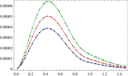
${\bar{E}}^{2}\,{\bar{R}}({\bar{E}})$

${\bar{E}}$

Figure 1: The transition probability rate of the rotating Unruh-DeWitt detector that is coupled to the conventional, massless scalar field. The dots and the curves that simply link them represent numerical results arrived at from the computation of the integral (8) along the rotating trajectory. The curves correspond to the following three values of the quantity $\sigma\,\Omega=0.325$ (in blue), $0.350$ (in red) and $0.375$ (in green). The dots of an alternate color that appear on the curves denote the numerical results that have been obtained by another method which I shall describe below [they actually correspond to the sum (24)]. Clearly, the results from the two methods match very well.

I should mention here that, in order to check the accuracy of the numerical procedure that I have used to evaluate the integral (8) for the rotating trajectory, I have compared the results from the numerical code with the analytical one [viz. Eq. (12)] that is available for the case of the uniformly accelerated detector. This comparison clearly indicates that the numerical procedure I have adopted to evaluate the integral (8) is quite accurate gutti-2011 .

In the discussion above, I had arrived at the response of the rotating detector by evaluating the Fourier transform of the Wightman function with respect to the differential proper time $u$ in the frame of the detector. In this case, evidently, I had first summed over the normal modes (to arrive at the Wightman function) before evaluating the integral over the differential proper time. I shall now rederive the result by changing the order of these procedures. I shall express the Wightman function as a sum over the normal modes and first evaluate the integral over the differential proper time before computing the sum. This method proves to be helpful later when I shall consider the Planck scale effects on the rotating detector. As I shall illustrate, the method can be easily extended to cases wherein the scalar field is described by a modified dispersion relation.

I shall start by working in the cylindrical polar coordinates, say, $(t,\rho,\theta,z)$, instead of the cartesian coordinates, since they prove to be more convenient. In terms of the cylindrical coordinates, the trajectory (13) of the rotating detector can be written in terms of the proper time $\tau$ as follows:

$${\tilde{x}}(\tau)=\left(\gamma\,\tau,\,\sigma,\,\gamma\,\Omega\,\tau,\,0\right).$$ (15)

Using well established properties of the Bessel functions, it is straightforward to show that, along the trajectory of the rotating detector, the standard Minkowski Wightman function (9) can be written as

$$G^{+}(u)=\sum^{\infty}_{m=-\infty}\,\int\limits^{\infty}_{0}\frac{{\rm d}q\,q}{\left(2\,\pi\right)^{2}}\,\int\limits^{\infty}_{-\infty}\frac{{\rm d}k_{z}}{\left(2\,\omega\right)}\,J_{m}^{2}(q\,\sigma)\;{\rm e}^{-i\,\gamma\,\left(\omega-m\,\Omega\right)\,u},$$ (16)

where $J_{m}(q\,\sigma)$ denote the Bessel functions of order $m$, with $\omega$ being given by

$$\omega=\left(q^{2}+k_{z}^{2}\right)^{1/2}.$$ (17)

One can then immediately express the corresponding transition probability rate of the rotating detector as [cf. Eq. (8)]

$$R(E)=\sum^{\infty}_{m=-\infty}\,\int\limits^{\infty}_{0}\frac{{\rm d}q\,q}{2\,\pi}\;\int\limits^{\infty}_{-\infty}\;\frac{{\rm d}k_{z}}{2\,\omega}\,J_{m}^{2}(q\,\sigma)\;\delta^{(1)}\left[E+\gamma\,\left(\omega-m\,\Omega\right)\right].$$ (18)

Recall that, $E>0$, $\omega\geq 0$ (as is appropriate for positive frequency modes), and I have assumed that $\Omega$ is a positive definite quantity as well. Hence, the delta function in the above expression will be non-zero only when $m\geq{\bar{E}}$, where ${\bar{E}}=E/\left(\gamma\,\Omega\right)$ is the dimensionless energy. Due to this reason, the response of the detector simplifies to

$$R({\bar{E}})=\sum^{\infty}_{m\geq{\bar{E}}}\,\int\limits^{\infty}_{0}\frac{{\rm d}q\,q}{2\,\pi}\;\int\limits^{\infty}_{-\infty}\frac{{\rm d}k_{z}}{2\,\omega}\;J_{m}^{2}(q\,\sigma)\;\left[\frac{\delta^{(1)}(k_{z}-\kappa_{z})}{\gamma\,\left|\left({\rm d}\omega/{\rm d}k_{z}\right)\right|_{\kappa_{z}}}\right],$$ (19)

where $\kappa_{z}$ are the two roots of $k_{z}$ from the following equation:

$$\omega=\left(m-{\bar{E}}\right)\,\Omega.$$ (20)

The roots are given by

$$\kappa_{z}=\pm\left(\lambda^{2}-q^{2}\right)^{1/2},$$ (21)

where, for convenience, I have set

$$\lambda={\bar{\lambda}}\,\Omega=\left(m-{\bar{E}}\right)\,\Omega.$$ (22)

Since both the positive and negative roots of $\kappa_{z}$ contribute equally, the dimensionless transition probability rate of the rotating detector can be obtained to be

$${\bar{R}}({\bar{E}})=\sigma\,R({\bar{E}})=\frac{\sigma}{2\,\pi\,\gamma}\,\sum^{\infty}_{m\geq{\bar{E}}}\,\int\limits_{0}^{\lambda}\;{\rm d}q\;q\;\left[\frac{J_{m}^{2}(q\,\sigma)}{\left(\lambda^{2}-q^{2}\right)^{1/2}}\right],$$ (23)

where I have set the upper limit on $q$ to be $\lambda$ as $\kappa_{z}$ is a real quantity [cf. Eq. (21)]. I find that the integral over $q$ can be expressed in terms of the hypergeometric functions (see, for instance, Ref. prudnikov-1986 ). Therefore, the transition probability rate of the rotating detector can be written as

$${\bar{R}}({\bar{E}}) = \frac{1}{2\,\pi\,\gamma}\ \sum^{\infty}_{m\geq{\bar{E}}}\,\frac{\left(\sigma\,\Omega\,{\bar{\lambda}}\right)^{(2\,m+1)}}{\Gamma\left(2\,m+2\right)}$$ (24)

$$\times\,_{1}F_{2}\left[m+(1/2);\,m+(3/2),2\,m+1;\,-\left(\sigma\,\Omega\,{\bar{\lambda}}\right)^{2}\right],$$

where ${}_{1}F_{2}\left(a;b,c;x\right)$ denotes the hypergeometric function, while $\Gamma(x)$ is the usual Gamma function. Though it does not seem to be possible to arrive at a closed form expression for this sum, the sum converges very quickly, and hence proves to be easy to evaluate numerically. In Fig. 1, I have plotted the numerical results for the above sum for the same values of the linear velocity $\sigma\,\Omega$ for which I had plotted the results obtained from Fourier transforming the Wightman function (14) along the rotating trajectory. The figure clearly indicates that the results from the two different methods match each other rather well.

2.2 Are detectors sensitive to the particle content of the field?

In order to clearly understand as to what detectors detect, I shall compare the response of detectors with the results from more conventional probes of the vacuum structure of the quantum fields, such as the approaches based on the Bogolubov transformations and the effective Lagrangian sriram-2002a . However, before carrying out such a comparison, let me say a few words briefly explaining these two other approaches.

Consider a quantum field that can be decomposed in terms of two complete sets of normal modes. These two sets of modes can be related to each other through the Bogolubov transformations, which are essentially characterized by two coefficients often referred to as $\alpha$ and $\beta$ bogolubov-1958 . Moreover, the particle content of the field is determined by the Bogolubov coefficient $\beta$. In a gravitational background, the Bogolubov transformations can either relate the modes of a quantum field at two different times in the same coordinate system or the modes in two different coordinate systems covering the same region of spacetime. When the Bogolubov coefficient $\beta$ is non-zero, in the latter context, such a result is normally interpreted as implying that the quantization in the two coordinate systems are inequivalent fulling-1973 . Whereas, in the former context, a non-zero $\beta$ is attributed to the production of particles by the background gravitational field qft-cb-reviews . Similarly, in an electromagnetic background, a non-zero $\beta$ relating the modes of a quantum field at different times (in a particular gauge) implies that the background leads to pair creation texts-qft-emb .

In the effective Lagrangian approach, one essentially integrates out the degrees of freedom associated with the quantum field, thereby arriving at an effective action describing the classical background heisenberg-1936 ; schwinger-1951 . An imaginary part to the effective Lagrangian unambiguously suggests the decay of the quantum vacuum, i.e. the production of particles corresponding to the quantum field. The real part of the effective Lagrangian can be related to the extent of polarization of the vacuum caused by the classical background. While the effective Lagrangian approach is powerful, since it involves computing a path integral, it often proves to be technically difficult to evaluate.

In Tab. 1, to illustrate the conclusions I wish to draw about the response of detectors, I have tabulated the results one obtains in a handful of different situations. I have listed whether the Bogolubov coefficient $\beta$, the response of the detector [or, more precisely, the transition probability $P(E)$] and the real and the imaginary parts of the effective Lagrangian ${\cal L}_{\rm eff}$ are zero or non-vanishing in these contexts. Apart from the results in the non-inertial frames in flat spacetime, I have compared the results between the Casimir plates, and different types of electromagnetic backgrounds.

	Detector	Bogolubov	Effective
	response	coefficient	Lagrangian
	$P(E)$	$\beta$	${\rm Re.}~{}{\cal L}_{\rm eff}\quad{\rm Im.}~{}{\cal L}_{\rm eff}$
In inertial coordinates	$0$	$0$	$\!\!\!\!0\qquad\qquad\;\;0$
In Rindler coordinates	$\neq 0$	$\neq 0$	$\!\!\!\!0\qquad\qquad\;\;0$
In rotating coordinates	$\neq 0$	$0$	$\!\!\!\!0\qquad\qquad\;\;0$
Between Casimir plates	$0$	$0$	$\!\!\!\!\!\!\!\neq 0\qquad\quad\;\;\;\,0$
In a time-dependent	$\neq 0$	$\neq 0$	$\!\!\!\!\,\neq 0\qquad\quad\,\,\neq 0$
electric field
In a time-independent	$\;\,\neq 0$	$\neq 0$	$\!\!\!\!\,\neq 0\qquad\quad\,\,\neq 0$
electric field
In a time-independent	$0$	$0$	$\!\!\!\!\!\!\!\neq 0\qquad\quad\;\;\;\,0$
magnetic field

Table 1: A comparison of the response of a detector with the results from more formal probes of the vacuum structure of the quantum field—viz. the Bogolubov transformations and the effective Lagrangian approaches—in a variety of situations. Note that, in the case of the time-independent electric field background, actually, the Bogolubov coefficient $\beta$ is trivially zero. I refer here to particle production that can occur in such a background due to the phenomenon called Klein paradox klein-p . I should also add that, in electromagnetic backgrounds, the coupling of the detector to the quantum field (say, a complex scalar field) has to be intrinsically non-linear in order to preserve gauge-invariance sriram-1999 .

Let me first consider the case of the non-inertial coordinates in flat spacetime. The Bogolubov coefficient $\beta$ relating the Rindler modes and the Minkowski modes turns out to be non-zero and, in fact, the expectation value of the Rindler number operator in the Minkowski vacuum yields a thermal spectrum as well fulling-1973 . In contrast, in the rotating coordinates, while the Bogolubov coefficient $\beta$ turns out to be zero letaw-1981a , as we have seen, the detector responds non-trivially. Also, in both these cases, one can show that the effective Lagrangian vanishes identically—in fact, this is true even in the case of the Rindler coordinates, wherein the Bogolubov coefficient $\beta$ proves to be non-zero sriram-2002a . Evidently, the response of a detector can be non-zero even when the Bogolubov coefficient $\beta$ and the effective Lagrangian vanish identically. Clearly, the response of a detector does not necessarily reflect the particle content of the quantum field.

Let me now turn to the response of the detector between Casimir plates and in electromagnetic backgrounds. It is well known that Casimir plates and a time-independent magnetic field lead to vacuum polarization, but not to particle production. One finds that an inertial detector does not respond in these two backgrounds. In contrast, it is found that even an inertial detector responds in an electric field background, whether time-dependent or otherwise. It is easy to argue that, in a time-dependent electric field, the evolving modes will excite the inertial detector sriram-1999 ; sriram-2002a . Whereas, in a time-independent electric field of sufficient strength, modes of positive norm that have negative frequencies (which lead to the so-called Klein paradox and associated pair production sriram-2002a ; klein-p , as is also reflected by the imaginary part of the effective Lagrangian schwinger-1951 ) are found to be responsible for a non-vanishing response of an inertial detector. These clearly suggest that, irrespective of the nature of its trajectory, a detector will respond whenever particle production takes place. In that sense a detector is sensitive to particle production. Further, if one restricts the motion of the detector to inertial trajectories, then the effects due to non-inertial motion can be avoided and, in such cases, the detector response will be non-zero only when particle production takes place. However, unlike in flat spacetime or classical electromagnetic backgrounds, there exists no special frame of reference in a classical gravitational background and all coordinate systems have to be treated equivalently. This aspect of the detector proves to be a major constraint in being able to utilize it to investigate the phenomenon of particle production in a curved spacetime davies-1984 ; particles-cst .

3 ‘Inversion of statistics’ in odd dimensions

We had seen that the response of a uniformly accelerating monopole detector that is coupled to a quantized massless scalar field is characterized by a Planckian distribution when the field is assumed to be in the Minkowski vacuum [cf. Eq. (12)]. However, it has been noticed that this result is true only in even-dimensional flat spacetimes and it has been shown that a Fermi-Dirac factor (rather than a Bose-Einstein factor) appears in the response of the accelerated detector when the dimensionality of spacetime is odd detectors-odd-std . Recall that the Unruh-DeWitt detector is coupled linearly to the quantum scalar field. Over the years, motivated by different reasons, there have also been efforts in the literature to investigate the response of detectors that are coupled non-linearly to the quantum field detectors-nlc ; suzuki-1997 ; sriram-1999 . It will be interesting to examine whether the non-linearity of the coupling affects the result in odd-dimensional flat spacetimes that I mentioned above.

3.1 Response of non-linearly coupled detectors

Consider a detector that is interacting with a real scalar field $\phi$ through the non-linear interaction Lagrangian suzuki-1997

$${\cal L}_{\rm int}[\phi({\tilde{x}})]={\bar{c}}\,m(\tau)\;\phi^{n}\left[{\tilde{x}}(\tau)\right],$$ (25)

where ${\bar{c}}$, $m(\tau)$ and ${\tilde{x}}(\tau)$ are the same quantities that we had encountered earlier in the context of the Unruh-DeWitt detector. The quantity $n$ is a positive integer that denotes the index of non-linearity of the coupling. Let me assume that the quantum field ${\hat{\phi}}$ is initially in the vacuum state $\left|0\right\rangle$. The transition amplitude of the non-linearly coupled detector from the ground to an excited state can be written as

$$A_{n}(E)=M\,\int\limits_{-\infty}^{\infty}{\rm d}\tau\,{\rm e}^{i\,E\,\tau}\,\left\langle\psi\right|\,{\hat{\phi}}^{n}[{\tilde{x}}(\tau)]\,\left|0\right\rangle,$$ (26)

where $\left|\psi\right\rangle$ is the final state of the field, and $M$ and $E$ are defined in the same fashion as in the case of the Unruh-Dewitt detector.

It is important to notice that the transition amplitude $A_{n}(E)$ above involves products of the quantum field ${\hat{\phi}}$ at the same spacetime point. Because of this reason, one will encounter divergences when evaluating this transition amplitude. In order to avoid these divergences, I shall normal order the operators in the matrix element in the transition amplitude $A_{n}(E)$ with respect to the Minkowski vacuum suzuki-1997 . In other words, rather than the expression (26), I shall assume that the transition amplitude is instead given by

$${\bar{A}}_{n}(E)=\int\limits_{-\infty}^{\infty}{\rm d}\tau\,{\rm e}^{i\,E\,\tau}\,\left\langle\psi\right|:{\hat{\phi}}^{n}[{\tilde{x}}(\tau)]:\left|0\right\rangle,$$ (27)

where the colons denote normal ordering with respect to the Minkowski vacuum. Then, the transition probability of the detector to all possible final states $\left|\psi\right\rangle$ of the quantum field can be written as

$$P_{n}(E)=\sum_{|\psi\rangle}{|{\bar{A}}_{n}(E)|}^{2}=\int\limits_{-\infty}^{\infty}{\rm d}\tau\,\int\limits_{-\infty}^{\infty}{\rm d}\tau^{\prime}\,{\rm e}^{-i\,E\,(\tau-\tau^{\prime})}\;G_{n}\left[{\tilde{x}}(\tau),{\tilde{x}}(\tau^{\prime})\right],$$ (28)

where $G_{n}\left[{\tilde{x}}(\tau),{\tilde{x}}(\tau^{\prime})\right]$ is the $(2\,n)$-point function defined as

$$G_{n}\left[{\tilde{x}}(\tau),{\tilde{x}}(\tau^{\prime})\right]=\left\langle 0\right|:{\hat{\phi}}^{n}\left[{\tilde{x}}(\tau)\right]:\,:{\hat{\phi}}^{n}\left[{\tilde{x}}(\tau^{\prime})\right]:\left|0\right\rangle.$$ (29)

In situations where the $(2\,n)$-point function $G_{n}\left[{\tilde{x}}(\tau),{\tilde{x}}(\tau^{\prime})\right]$ is invariant under time translations in the frame of the detector, I can define a transition probability rate for the detector as follows:

$$R_{n}(E)=\int\limits_{-\infty}^{\infty}{\rm d}u\;{\rm e}^{-i\,E\,u}\;G_{n}(u),$$ (30)

where, as earlier, $u=\tau-\tau^{\prime}$.

3.2 Odd statistics in odd dimensions for odd couplings

Let me now assume that the quantum scalar field ${\hat{\phi}}$ is in the Minkowski vacuum. In this case, the $(2\,n)$-point function $G_{n}\left({\tilde{x}},{\tilde{x}^{\prime}}\right)$ reduces to

$$G_{n}\left({\tilde{x}},{\tilde{x}^{\prime}}\right)=n!\,\left[G^{+}\left({\tilde{x}},{\tilde{x}^{\prime}}\right)\right]^{n},$$ (31)

where $G^{+}\left({\tilde{x}},{\tilde{x}^{\prime}}\right)$ denotes the Wightman function in the Minkowski vacuum. The Wightman function (9) that I had quoted earlier had corresponded to the result in $(3+1)$-spacetime dimensions. In $(D+1)$ spacetime dimensions [and for $(D+1)\geq 3$], the Wightman function for a massless scalar field in the Minkowski vacuum is given by detectors-odd-std

$$G^{+}({\tilde{x}},{\tilde{x}^{\prime}})=\frac{C_{D}}{\biggl{\{}(-1)\;\left[(t-t^{\prime}-i\,\epsilon)^{2}-|{\bm{x}}-{\bm{x}}^{\prime}|^{2}\right]\biggr{\}}^{(D-1)/2}},$$ (32)

where it should be evident that ${\bm{x}}\equiv\left(x^{1},x^{2},\ldots,x^{D}\right)$, while the quantity $C_{D}$ is given by

$$C_{D}=\Gamma\left[(D-1)/2\right]/\left[4\,\pi^{(D+1)/2}\right]$$ (33)

with $\Gamma\left[(D-1)/2\right]$ denoting the Gamma function.

Now, the trajectory of a detector accelerating uniformly along the $x^{1}$ direction with a proper acceleration $g$ is given by

$${\tilde{x}}(\tau)=g^{-1}\,\left[{\rm sinh}\,(g\,\tau),\,{\rm cosh}\,(g\,\tau),\,0,\,0,\ldots,\,0\right],$$ (34)

where $\tau$ is the proper time in the frame of the detector. On substituting this trajectory in the Minkowski Wightman function (32), I obtain that detectors-odd-std

$$G^{+}(u)=\frac{C_{D}\;(g/2\,i)^{(D-1)}}{\biggl{\{}{\rm sinh}\left[\left(g\,u/2\right)-i\,\epsilon\right]\biggr{\}}^{(D-1)}}.$$ (35)

Therefore, along the trajectory of the uniformly accelerating detector, the $(2\,n)$-point function in the Minkowski vacuum (31) is given by

$$G_{n}(u)=\frac{n!\,C_{D}^{n}\;(g/2\,i)^{p}}{\biggl{\{}{\rm sinh}\left[(g\,u/2)-i\,\epsilon\right]\biggl{\}}^{p}},$$ (36)

where $p=(D-1)\,n$.

Upon substituting the $(2\,n)$-point function (36) in the expression (30) and carrying out the resulting integral gradshteyn-1980 , I find that the transition probability rate of the uniformly accelerated, non-linearly coupled detector can be written as sriram-2002b

$$R_{n}(E)=B(n,D)\;\;\left\{\begin{array}[]{l}\left(g^{p}/E\right)\;{\underbrace{\frac{1}{\exp\,(2\,\pi\,E/g)-1}}}\;\prod\limits_{l=0}^{(p-2)/2}\left[l^{2}+(E/g)^{2}\right]\\ \qquad\quad\,\mbox{Bose-Einstein factor}\qquad\qquad\qquad\quad\;\mbox{when $p$ is even},\\ g^{p-1}\;{\underbrace{\frac{1}{\exp\,(2\,\pi\,E/g)+1}}}\;\prod\limits_{l=0}^{(p-3)/2}\biggl{\{}\left[(2\,l+1)/2\right]^{2}+(E/g)^{2}\biggr{\}}\\ \qquad\quad\;\mbox{Fermi-Dirac factor}\qquad\qquad\qquad\qquad\mbox{when $p$ is odd,}\end{array}\right.$$ (37)

where the quantity $B(n,D)$ is given by

$$B(n,D)=2\,\pi\,n!\;C_{D}^{n}/\Gamma(p).$$ (38)

When $(D+1)$ is even, $p$ is even for all $n$ and, hence, a Bose-Einstein factor will always arise in the response of the uniformly accelerated detector in an even-dimensional flat spacetime. Whereas, when $(D+1)$ is odd, evidently, $p$ will be odd or even depending on whether $n$ is odd or even. Therefore, in an odd-dimensional flat spacetime, a Fermi-Dirac factor will arise in the detector response when $n$ is odd (as in the case of the Unruh-DeWitt detector), but a Bose-Einstein factor will appear when $n$ is even!

Let me make three clarifying comments regarding the curious result I have obtained above. To begin with, the temperature associated with the Bose-Einstein and the Fermi-Dirac factors that appear in the response of the non-linearly coupled detector is the standard Unruh temperature, viz. $g/(2\,\pi)$. Moreover, the response of the detector is characterized completely by either a Bose-Einstein or a Fermi-Dirac distribution only in situations wherein $p<3$. When $p\geq 3$, apart from a Bose-Einstein or a Fermi-Dirac factor, the detector response contains a term which is polynomial in $E/g$. Lastly, plots of the transition probability rate of the detector suggest that, though the characteristic response of the detector alternates between the Bose-Einstein and the Fermi-Dirac factors as we go from one $D$ to another for odd $n$ [or from one $n$ to another when $(D+1)$ is odd], the complete spectra themselves exhibit a smooth dependence on the index of non-linearity of the coupling as well as the dimension of spacetime (in this context, see the figures in Ref. sriram-2002b ).

3.3 Nature of the odd statistics

Despite its interesting character, the ‘inversion of statistics’ encountered in the response of the detector in odd dimensions for odd couplings seems to be only apparent. It is well known that, in the frame of the uniformly accelerating detector, the Wightman function in the Minkowski vacuum (35) is skew-periodic in imaginary proper time with a period corresponding to the inverse of the Unruh temperature wfn-sp , i.e.

$$G^{+}(u)=G^{+}\left[-u+(2\,\pi\,i/g)\right].$$ (39)

This property is known as the Kubo-Martin-Schwinger (KMS) condition, as is applicable to scalar fields. Note that the above property is, in fact, satisfied by the Minkowski Wightman function in all dimensions detectors-odd-std . Since the $(2\,n)$-point function in the Minkowski vacuum is proportional to the $n$th power of the Wightman function, obviously, in the frame of the accelerated detector, the $(2\,n)$-point function will also be skew-periodic in imaginary proper time for all $n$ and $D$ [cf. Eq. (36)]. In other words, the $(2\,n)$-point function satisfies the KMS condition (as is required for a scalar field) for all $D$ and $n$. This implies that the appearance of the Fermi-Dirac factor (instead of the expected Bose-Einstein factor) for odd $(D+1)$ and $n$ simply reflects a peculiar aspect of the detector rather than indicate a fundamental shift in the field theory in such situations detectors-odd-std ; sriram-2002b ; sriram-2003 .

4 Detecting Planck scale effects

Consider a typical mode that constitutes Hawking radiation at future null infinity around a collapsing black hole. As one traces such a mode back to the past null infinity where the initial conditions are imposed on the quantum field, it is found that the energy of the mode turns out to be way beyond the Planck scale tpp-bhe . (This feature seems to have been originally noticed in Ref. wald-1976 ; in this context, also see Ref. wald-1984 .) In fact, due to the rapid, virtually exponential expansion, a similar phenomenon is encountered in the context of the inflationary scenario. One finds that scales of cosmological interest can be comparable to the Planck scale at very early times when the initial conditions are imposed during inflation tpp-ic . While the possible Planck scale corrections to Hawking radiation and the perturbations generated during inflation have cornered most of the attention tpp-bhe ; tpp-ic , the Planck scale effects on a variety of non-perturbative, quantum field theoretic effects in flat as well as curved spacetimes have been investigated as well (see, for example, Refs. srini-1998 ; jacobson-2001 ; other-e ). In the absence of a viable quantum theory of gravity, it becomes imperative to extend such phenomenological analyses to as many physical situations as possible (in this context, see Ref. hossenfelder-2009 , and references therein).

The Unruh effect has certain similarities with Hawking radiation from black holes. Due to this reason, the Unruh effect and its variants provide another interesting domain to study the quantum gravitational effects psm-ue . But, due to the lack of a workable quantum theory of gravity, to investigate the Planck scale effects, one is forced to consider phenomenological models constructed by hand. These models attempt to capture one or more features expected of the actual effective theory obtained by integrating out the gravitational degrees of freedom. The approach based on modified dispersion relations has been extensively considered both in the context of black holes and inflationary cosmology. In this approach, a fundamental scale is effectively introduced into the theory by breaking local Lorentz invariance (see, for instance, Refs. jacobson-2001 ; lvm-reviews ). It should be clarified that there does not exist any experimental or observational reason to believe that Lorentz invariance could be violated at high energies. Nevertheless, theoretically, these models prove to be attractive because of the fact that they permit quantum field theories to be constructed and calculations to be carried out in a consistent fashion.

In this section, I shall adopt the approach due to the modified dispersion relations to analyze the Planck scale corrections to the response of the rotating Unruh-DeWitt detector in flat spacetime. As I shall show, the rotating trajectory turns out to be a special case wherein the transition probability rate of the rotating detector can be defined in precisely the same fashion as I had done earlier in the case of the canonical scalar field governed by the linear dispersion relation. I shall illustrate that the response of the rotating detector can be computed exactly, although, numerically, even when the field it is coupled to is described by a non-linear dispersion relation.

4.1 Scalar field governed by a modified dispersion relation

I shall be interested in calculating the response of the rotating detector when it is coupled to a massless scalar field that is governed by a modified dispersion relation of the following form:

$$\omega=k\,\left[1+a\,\left(k/k_{{}_{\rm P}}\right)^{2}\right]^{1/2}.$$ (40)

The quantity $\omega$ is the frequency corresponding to the mode ${\bm{k}}$, $k=|{\bm{k}}|$ and $k_{{}_{\rm P}}$ denotes the fundamental scale (that I shall assume to be of the order of the Planck scale) at which the deviations from the linear dispersion relation become important. Note that $a$ is a dimensionless constant whose magnitude is of order unity, and the above dispersion relation is super-luminal or sub-luminal depending upon whether $a$ is positive or negative. Clearly, if I can evaluate the Wightman function associated with the quantized scalar field described by the non-linear dispersion relation (40), I may then be able to evaluate the corresponding transition probability rate of the rotating detector as I had carried out originally. However, unlike the standard case, it turns out to be difficult to even arrive at an analytical expression for the Wightman function of such a scalar field. Therefore, I shall make use of the second method that I had adopted earlier to evaluate the response of the rotating detector—I shall first integrate over the differential proper time and then numerically sum over the normal modes to arrive at the transition probability rate.

The equation of motion of the scalar field $\phi$ that is described by the dispersion relation (40) is given by

$$\Box\,\phi+\frac{a}{k_{{}_{\rm P}}^{2}}\,\nabla^{2}\,\left(\nabla^{2}\,\phi\right)=0,$$ (41)

where $\Box$ is the d’Alembertian corresponding to the four dimensional Minkowski spacetime, while $\nabla^{2}$ is the three dimensional, spatial Laplacian. Evidently, the first term in the above equation is the standard one. The non-linear term in the dispersion relation is responsible for the second term. Such terms can be generated by adding suitable terms to the original action describing the scalar field jacobson-2001 ; lvm-reviews . While these additional terms preserve rotational invariance, they break Lorentz invariance. In fact, this property is common to all the theories that are described by a non-linear dispersion relation. It is obvious that the normal modes of such a scalar field in flat spacetime remain plane waves as in the standard case, but with the frequency and the wavenumber related by the modified dispersion relation. Moreover, the quantization of the scalar field can be carried out in the same fashion. It is straightforward to show that, in the Minkowski vacuum, the Wightman function for any such field in $(3+1)$-spacetime dimensions can be expressed as (see, for example, Ref. jacobson-2001 )

$$G^{+}_{{}_{\rm M}}({\tilde{x}},{\tilde{x}}^{\prime})=\int\frac{{\rm d}^{3}{\bm{k}}}{(2\,\pi)^{3}\,2\,\omega}\,{\rm e}^{-i\,\omega\,(t-t^{\prime})}\,{\rm e}^{i\,{\bm{k}}\cdot\,({\bm{x}}-{\bm{x}}^{\prime})}$$ (42)

with $\omega$ being related to $k=|{\bm{k}}|$ by the given non-linear dispersion relation.

4.2 Response of the rotating detector

For a scalar field governed by a modified dispersion relation, using the expression (42) for the corresponding Wightman function, one can immediately show that, along the rotating trajectory, the function can be expressed exactly as in Eq. (16), with the frequency $\omega$ being related to the wavenumbers $q$ and $k_{z}$ by the non-linear dispersion relation. Clearly, in such a case, the transition probability rate of the detector will again be given by Eq. (19) with $\omega$ suitably defined. It is important to recognize that the result is actually applicable for any non-linear dispersion relation gutti-2011 .

Let me now evaluate the response of the rotating detector for the dispersion relation (40). In such a case, $\omega$ is related to the wavenumbers $q$ and $k_{z}$ as follows:

$$\omega=\left(q^{2}+k_{z}^{2}\right)^{1/2}\;\left[1+\frac{a}{k_{{}_{\rm P}}^{2}}\,\left(q^{2}+k_{z}^{2}\right)\right]^{1/2}.$$ (43)

Also, one can show that the roots $\kappa_{z}$ [from Eq. (20)] are given by

$$\kappa_{z}^{2}=\pm\frac{k_{{}_{\rm P}}^{2}}{2\,a}\,\left(1+\frac{4\,a\,\lambda^{2}}{k_{{}_{\rm P}}^{2}}\right)^{1/2}-\frac{k_{{}_{\rm P}}^{2}}{2\,a}-q^{2},$$ (44)

with $\lambda$ defined as in Eq. (22). It ought to be noted that $\kappa_{z}^{2}$ has to be positive definite, since $\kappa_{z}$ is a real quantity.

Let me first consider the super-luminal case when $a$ is positive. When, say, $a=1$, the two roots that contribute to the delta function in Eq. (19) can be written as

$$\kappa_{z}=\pm\left(\lambda_{+}^{2}-q^{2}\right)^{1/2},$$ (45)

where $\lambda_{+}^{2}$ is given by the expression

$$\lambda_{+}^{2} = \frac{k_{{}_{\rm P}}^{2}}{2}\,\left[\left(1+\frac{4\,\lambda^{2}}{k_{{}_{\rm P}}^{2}}\right)^{1/2}-1\right]$$ (46)

$$= \frac{{\bar{\lambda}}_{+}^{2}}{\sigma^{2}}=\frac{{{\bar{k}}_{{}_{\rm P}}}^{2}}{2\,\sigma^{2}}\,\left[\left(1+\frac{4\,(\sigma\,\Omega\,{\bar{\lambda}})^{2}}{{\bar{k}}_{{}_{\rm P}}^{2}}\right)^{1/2}-1\right].$$

Note that ${\bar{k}}_{{}_{\rm P}}=\sigma\,k_{{}_{\rm P}}$ denotes the dimensionless fundamental scale and the sub-script in $\lambda_{+}$ refers to the fact that I am considering a super-luminal dispersion relation. Further, as $\kappa_{z}$ is real, I require that $q\leq\lambda_{+}$. As in the standard case, the positive and negative roots of $\kappa_{z}$ above contribute equally. Therefore, the response of the rotating detector is given by

$${\bar{R}}({\bar{E}})=\sigma\,R({\bar{E}})=\frac{\sigma}{2\,\pi\,\gamma}\,\sum^{\infty}_{m\geq{\bar{E}}}\,\left(1+\frac{2\,\lambda_{+}^{2}}{k_{{}_{\rm P}}^{2}}\right)^{-1}\;\int\limits_{0}^{\lambda_{+}}\;{\rm d}q\;q\;\left[\frac{J_{m}^{2}(q\,\sigma)}{\left(\lambda_{+}^{2}-q^{2}\right)^{1/2}}\right],$$ (47)

and the integral over $q$ can be carried out as in the standard case to arrive at the result

$${\bar{R}}({\bar{E}}) = \frac{1}{2\,\pi\,\gamma}\ \sum^{\infty}_{m\geq{\bar{E}}}\,\frac{{\bar{\lambda}}_{+}^{(2\,m+1)}}{\Gamma\,\left(2\,m+2\right)}\;\left(1+\frac{2\,{{\bar{\lambda}}_{+}}^{2}}{{\bar{k}}_{{}_{\rm P}}^{2}}\right)^{-1}$$ (48)

$$\times\,_{1}F_{2}\left[m+(1/2);\,m+(3/2),2\,m+1;-{\bar{\lambda}}_{+}^{2}\right].$$

It should be emphasized here that this result for the transition probability rate is exact and no approximations have been made in arriving at the expression.

Since the Planck scale is expected to be orders of magnitude beyond the scales probed by experiments, the quantity ${\bar{k}}_{{}_{\rm P}}$ is expected to be large. It is clear that, as ${\bar{k}}_{{}_{\rm P}}\to\infty$, ${\bar{\lambda}}_{+}\to\sigma\,\Omega\,{\bar{\lambda}}$ and, hence, the transition transition probability rate (48) reduces to the expression that I had arrived at earlier for the standard dispersion relation [viz. Eq. (24)], as required. Let me now evaluate the Planck scale corrections to the standard result by expanding the transition probability rate (48) in terms of $\lambda/k_{{}_{\rm P}}$ and retaining terms upto ${\cal O}[\left(\lambda/k_{{}_{\rm P}}\right)^{2}]$. Note that, in such a case, $\lambda_{+}$ reduces to

$$\lambda_{+}\simeq\lambda\,\left(1-\frac{\lambda^{2}}{2\,k_{{}_{\rm P}}^{2}}\right),$$ (49)

so that I have

$$\lambda_{+}^{(2\,m+1)}\simeq\lambda^{(2\,m+1)}-(2\,m+1)\,\frac{\lambda^{(2\,m+3)}}{2\,k_{{}_{\rm P}}^{2}}$$ (50)

and

$$\left(1+\frac{2\,\lambda_{+}^{2}}{k_{{}_{\rm P}}^{2}}\right)^{-1}\simeq 1-\frac{2\,\lambda^{2}}{k_{{}_{\rm P}}^{2}}.$$ (51)

Moreover, in the limit of our interest, the hypergeometric function in Eq. (48) can be written as

$$\!\!\!\!\!\!\!\!\!\!{}_{1}F_{2}\left[m+(1/2);\,m+(3/2),\,2\,m+1;\,-{\bar{\lambda}}_{+}^{2}\right]$$

$$\quad\simeq\,_{1}F_{2}\left[m+(1/2);\,m+(3/2),\,2\,m+1;\,-\left(\sigma\,\Omega\,{\bar{\lambda}}\right)^{2}\right]$$

$$\qquad+\,\frac{(\sigma\,\Omega\,{\bar{\lambda}})^{2}}{{\bar{k}}_{{}_{\rm P}}^{2}}\,\frac{[m+(1/2)]\;(\sigma\,\Omega\,{\bar{\lambda}})^{2}}{[m+(3/2)]\;(2\,m+1)}$$

$$\qquad\;\;\times\,_{1}F_{2}\left[m+(3/2);\,m+(5/2),\,2\,m+2;\,-\left(\sigma\,\Omega\,{\bar{\lambda}}\right)^{2}\right].$$ (52)

Upon using the above expansions, I obtain the response of the detector at ${\cal O}[\left(\lambda/k_{{}_{\rm P}}\right)^{2}]$ to be

$$\!\!\!\!\!\!\!\!\!\!\!\!\!\!\!\!\!\!\!\!\!\!\!\!{\bar{R}}({\bar{E}}) \simeq \frac{1}{2\,\pi\,\gamma}\,\sum^{\infty}_{m\geq{\bar{E}}}\,\frac{\left(\sigma\,\Omega\,{\bar{\lambda}}\right)^{(2\,m+1)}}{\Gamma\left(2\,m+2\right)}$$ (53)

$$\times\,_{1}F_{2}\left[m+(1/2);\,m+(3/2),\,(2\,m+1);\,-\left(\sigma\,\Omega\,{\bar{\lambda}}\right)^{2}\right]$$

$$-\,\frac{1}{2\,\pi\,\gamma}\,\frac{(\sigma\,\Omega\,{\bar{\lambda}})^{2}}{{\bar{k}}_{{}_{\rm P}}^{2}}\,\sum^{\infty}_{m\geq{\bar{\cal E}}}\,\frac{[m+(5/2)]\,\left(\sigma\,\Omega\,{\bar{\lambda}}\right)^{(2\,m+1)}}{\Gamma\left(2\,m+2\right)}$$

$$\times\,_{1}F_{2}\left[m+(1/2);\,m+(3/2),\,2\,m+1;\,-\left(\sigma\,\Omega\,{\bar{\lambda}}\right)^{2}\right]$$

$$+\,\frac{1}{2\,\pi\,\gamma}\,\frac{(\sigma\,\Omega\,{\bar{\lambda}})^{2}}{{\bar{k}}_{{}_{\rm P}}^{2}}\,\sum^{\infty}_{m\geq{\bar{E}}}\,\frac{[m+(1/2)]\;\left(\sigma\,\Omega\,{\bar{\lambda}}\right)^{(2\,m+3)}}{[m+(3/2)]\,(2\,m+1)\;\Gamma\left(2\,m+2\right)}$$

$$\times\;_{1}F_{2}\left[m+(3/2);\,m+(5/2),\,2\,m+2;\,-\left(\sigma\,\Omega\,{\bar{\lambda}}\right)^{2}\right].$$

Evidently, the first term in this expression corresponds to the conventional transition probability rate [cf. Eq. (24)], while the other two terms represent the leading corrections to the standard result.

Let me now turn to considering the sub-luminal dispersion relation. When $a$ is negative, say, $a=-1$, the roots $\kappa_{z}$ are given by

$$\kappa_{z}=\pm\left(\lambda_{-}^{2}-q^{2}\right)^{1/2}$$ (54)

with $\lambda_{-}^{2}$ defined as

$$(\lambda_{-}^{\pm})^{2} = \frac{k_{{}_{\rm P}}^{2}}{2}\,\left[1\pm\left(1-\frac{4\,\lambda^{2}}{k_{{}_{\rm P}}^{2}}\right)^{1/2}\right]$$ (55)

$$= \frac{({\bar{\lambda}}_{-}^{\pm})^{2}}{\sigma^{2}}=\frac{{\bar{k}}_{{}_{\rm P}}^{2}}{2\,\sigma^{2}}\,\Biggl{\{}1\pm\left[1-\frac{4\,(\sigma\,\Omega\,{\bar{\lambda}})^{2}}{{\bar{k}}_{{}_{\rm P}}^{2}}\right]^{1/2}\Biggr{\}},$$

where the minus sign in the sub-script represents that it corresponds to the sub-luminal case (i.e. when $a$ is negative), while the super-scripts denote the two different possibilities of $\lambda_{-}$. Just as in the super-luminal case (i.e. when $a=1$), I require $q\leq\lambda_{-}^{\pm}$, if $\kappa_{z}$ is to remain real. Moreover, note that, unlike the super-luminal case, there also arises an upper limit on the sum over $m$. I require that $\lambda\leq k_{{}_{\rm P}}/2$, in order to ensure that $\lambda_{-}^{\pm}$ is real. This corresponds to $m\leq{\bar{E}}+{\bar{k}}_{{}_{\rm P}}/(2\,\sigma\,\Omega)$. Therefore, for the sub-luminal dispersion relation, I find that I can write the response of the rotating detector as follows:

$${\bar{R}}({\bar{E}}) = \frac{1}{2\,\pi\,\gamma}\,\sum^{{\bar{E}}+{\bar{k}}_{{}_{\rm P}}/(2\,\sigma\,\Omega)}_{m\geq{\bar{E}}}\,\frac{\left({\bar{\lambda}}_{-}^{-}\right)^{(2\,m+1)}}{\Gamma(2\,m+2)}\,\left(\;\left|\,1-\frac{2\,({\bar{\lambda}}_{-}^{-})^{2}}{{\bar{k}}_{{}_{\rm P}}^{2}}\right|\;\right)^{-1}$$ (56)

$$\times\,_{1}F_{2}\left[m+(1/2);\,m+(3/2),\,2\,m+1;\,-\left({\bar{\lambda}}_{-}^{-}\right)^{2}\right]$$

$$+\,\frac{1}{2\,\pi\,\gamma}\,\sum^{{\bar{E}}+k_{{}_{\rm P}}/(2\,\sigma\,\Omega)}_{m\geq{\bar{E}}}\,\frac{\left({\bar{\lambda}}_{-}^{+}\right)^{2\,m+1}}{\Gamma\left(2\,m+2\right)}\,\left(\;\left|\,1-\frac{2\,({\bar{\lambda}}_{-}^{+})^{2}}{{\bar{k}}_{{}_{\rm P}}^{2}}\right|\;\right)^{-1}$$

$$\times\;_{1}F_{2}\left[m+(1/2);\,m+(3/2),\,2\,m+1;\,-\left({\bar{\lambda}}_{-}^{+}\right)^{2}\right].$$

The reason for the upper limit on $m$ as well as the origin of the second term in the above expression for the response of the rotating detector can be easily understood. The quantity $\omega$ is a monotonically increasing function of $q$ and $k_{z}$ in the case of the super-luminal dispersion relation. Because of this reason, there exist only two real roots of $k_{z}$ corresponding to a given $\omega$. Moreover, $\omega^{2}$ remains positive definite for all the modes. In contrast, in the sub-luminal case, after a rise, $\omega$ begins to decrease for sufficiently large values of $q$ and $k_{z}$. Actually, $\omega^{2}$ even turns negative at a suitably large value jacobson-2001 . It is this feature of the sub-luminal dispersion relation which leads to the upper limit on $m$, and the limit ensures that we avoid complex frequencies. (Such a cut-off can be achieved if I assume that, say, the detector is not coupled to modes with $m$ beyond a certain value, when the frequency turns complex.) There arise two additional two roots of $k_{z}$ which contribute to the detector response in the sub-luminal case as a result of the decreasing $\omega$ at large $q$ and $k_{z}$. The second term in the above transition probability rate of the rotating detector corresponds to the contributions from these two extra roots.

If one plots the result (48) for the response of the rotating detector when it is coupled to a field that is governed by a super-luminal dispersion relation, one finds that it does not differ from the standard result (as plotted in Fig. 1) even for an unnaturally small value of ${\bar{k}}_{{}_{\rm P}}$ such that, say, ${\bar{k}}_{{}_{\rm P}}/{\bar{E}}\simeq 10$. This implies that super-luminal dispersion relations do not alter the conventional result to any extent. It needs to be emphasized here that similar conclusions have been arrived at earlier in the context of black holes as well as inflationary cosmology. In these contexts, it has been shown that Hawking radiation and the inflationary perturbation spectra remain unaffected due to super-luminal modifications to the conventional, linear, dispersion relation tpp-bhe ; tpp-ic . In Fig. 2, I have plotted the transition probability rate (56) of the rotating Unruh-DeWitt detector corresponding to the sub-luminal dispersion relation that I have considered. I have plotted the result for a rather small value of ${\bar{k}}_{{}_{\rm P}}=50$. It is clear from the figure that the sub-luminal dispersion relation can lead to substantial modifications to the standard result. I believe that the modifications from the standard result will be considerably smaller (than exhibited in the figure) for much larger and more realistic values of ${\bar{k}}_{{}_{\rm P}}$ such that, say, ${\bar{k}}_{{}_{\rm P}}/{\bar{E}}>10^{10}$.

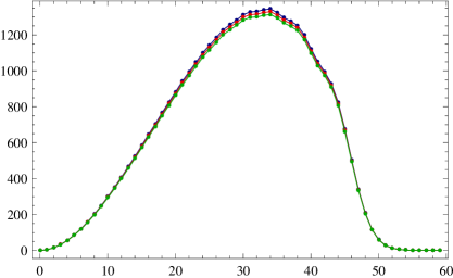
${\bar{E}}^{2}\,{\bar{R}}({\bar{E}})$

${\bar{E}}$

Figure 2: The transition probability rate of the rotating Unruh-DeWitt detector that is coupled to a massless scalar field governed by the modified dispersion relation (40) with $a=-1$. The dots and the curves linking them denote the numerical results for the same set of values for the quantity $\sigma\,\Omega$ (and the same choice of colors) that I had plotted in the previous figure. I have set ${\bar{k}}_{{}_{\rm P}}=50$, which is an extremely small value for ${\bar{k}}_{{}_{\rm P}}$. Evidently, for such a value, the modifications to the standard result (cf. Fig. 1) due to the sub-luminal dispersion relation is considerable. In fact, more realistic values of ${\bar{k}}_{{}_{\rm P}}$ would correspond to, say, ${\bar{k}}_{{}_{\rm P}}/{\bar{E}}>10^{10}$. However, numerically, it turns out to be difficult to sum the contributions in the expression (56) up to such large values of ${\bar{k}}_{{}_{\rm P}}$. It seems reasonable to conclude that the modifications to standard result due to the sub-luminal dispersion relation can be expected to be much smaller if one assumes ${\bar{k}}_{{}_{\rm P}}$ to be sufficiently large. Nevertheless, my analysis unambiguously points to the fact that, as is known to occur in other situations, a sub-luminal dispersion relation modifies the standard result considerably more than a similar super-luminal dispersion relation.

4.3 Rotating detector in the presence of a boundary

I shall now consider an interesting situation wherein I study the response of the rotating detector in the presence of an additional boundary condition that is imposed on the scalar field on a cylindrical surface in flat spacetime. Because of the symmetry of the problem, in this case too, the cylindrical coordinates turn out to be more convenient to work with.

It is well known that the time-like Killing vector associated with an observer who is rotating at an angular velocity $\Omega$ in flat spacetime becomes space-like for radii greater than $\rho_{{}_{\rm SL}}=1/\Omega$. Due to this reason, it has been argued that one needs to impose a boundary condition on the quantum field at a radius $\rho<\rho_{{}_{\rm SL}}$ when evaluating the response of a rotating detector davies-1996 . Curiously, in the presence of such a boundary, it was found that a rotating Unruh-DeWitt detector which is coupled to the standard scalar field ceases to respond. It is then interesting to examine whether this result holds true even when one assumes that the scalar field is governed by a modified dispersion relation.

In the cylindrical coordinates, along the rotating trajectory (15), the Wightman function corresponding to a scalar field that is assumed to vanish at, say, $\rho=\rho_{\ast}\;(<\rho_{{}_{\rm SL}})$, can be expressed as a sum over the normal modes of the field as follows davies-1996 :

$$G^{+}(u)=\sum\limits_{m=-\infty}^{\infty}\;\sum\limits_{n=1}^{\infty}\;\int\limits_{-\infty}^{\infty}\;\frac{{\rm d}k_{z}}{\left(2\,\pi\right)^{2}\,2\,\omega}\;\left[N\,J_{m}(\xi_{mn}\,\sigma/\rho_{\ast})\right]^{2}\;e^{-i\,\gamma\,\left(\omega-m\,\Omega\right)\,u},$$ (57)

where $\xi_{mn}$ denotes the $n$th zero of the Bessel function $J_{m}(\xi_{mn}\,\sigma/\rho_{\ast})$, while $N$ is a normalization constant that is given by

$$N=\frac{\sqrt{2}}{\rho_{\ast}\,|J_{m+1}(\xi_{mn})|}.$$ (58)

As in the situation without a boundary, $m$ is a real integer, whereas $k_{z}$ is a continuous real number. But, due to the imposition of the boundary condition at $\rho=\rho_{\ast}$, the spectrum of the radial modes is now discrete, and is described by the positive integer $n$. It should be pointed out that the expression (57) is in fact valid for any dispersion relation, with $\omega$ suitably related to the quantities $\xi_{mn}$ and $k_{z}$. For instance, in the case of the modified dispersion relation (40), the quantity $\omega$ is given by

$$\omega=\left(\frac{\xi_{mn}^{2}}{\rho_{\ast}^{2}}+k_{z}^{2}\right)^{1/2}\;\left[1+\frac{a}{k_{{}_{\rm P}}^{2}}\;\left(\frac{\xi_{mn}^{2}}{\rho_{\ast}^{2}}+k_{z}^{2}\right)\right]^{1/2},$$ (59)

where, it is evident that, while the overall factor corresponds to the standard, linear, dispersion relation, the term involving $a$ within the brackets arises due to the modifications to it. Since the Wightman function depends only $u$, the transition probability rate of the detector simplifies to

$$R(E)=\sum\limits_{m=-\infty}^{\infty}\;\sum\limits_{n=1}^{\infty}\;\int\limits_{-\infty}^{\infty}\;\frac{{\rm d}k_{z}}{2\,\pi\;\,2\,\omega}\;\left[N\,J_{m}(\xi_{mn}\,\sigma/\rho_{\ast})\right]^{2}\;\delta^{(1)}\left[E+\gamma\,\left(\omega-m\,\Omega\right)\right].$$ (60)

For exactly the same reasons that I had presented in the last section, the delta function in this expression can be non-zero only when $m>0$. In fact, the detector will respond only under the condition

$$m\,\Omega>\frac{\xi_{m1}}{\rho_{\ast}}\;\left(1+\frac{a}{k_{{}_{\rm P}}^{2}}\,\frac{\xi_{m1}^{2}}{\rho_{\ast}^{2}}\right)^{1/2},$$ (61)

where the right hand side is the lowest possible value of $\omega$ corresponding to $n=1$ and $k_{z}=0$. However, from the properties of the Bessel function, it is known that $\xi_{mn}>m$, for all $m$ and $n$ (see, for instance, Ref. abramowitz-1965 ). Therefore, when $a$ is positive, $\Omega\,\rho_{\ast}$ has to be greater than unity, if the rotating detector has to respond. But, this is not possible since I have assumed that the boundary at $\rho_{\ast}$ is located inside the static limit $\rho_{{}_{\rm SL}}=1/\Omega$. This is exactly the same conclusion that one arrives at in the standard case davies-1996 ; crispino-2008 .

Actually, it is easy to argue that the above conclusion would apply for all super-luminal dispersion relations. But, it seems that, under the same conditions, the rotating detector would be excited by a certain range of modes if I consider the scalar field to be described by a sub-luminal (such as, when $a<0$) dispersion relation! In fact, this aspect is rather easy to understand. Consider a frequency, say, $\omega$, associated with a mode through the linear dispersion relation. Evidently, a super-luminal dispersion relation raises the energy of all the modes, while the sub-luminal dispersion relation lowers it. Therefore, if the interaction of the detector with a standard field does not excite a particular mode of the quantum field, clearly, the mode is unlikely to be excited if its energy has been raised further, as in a super-luminal dispersion relation. However, the motion of the detector mode may be able to excite a mode of the field, if the energy of certain modes are lowered when compared to the standard case, as the sub-luminal dispersion relation does.

5 Finite time detectors

The response of detectors have always been studied for their entire history, viz. from the infinite past to the infinite future in the detector’s proper time. But, in any realistic situation, the detectors can be kept switched on only for a finite period of time and due to this reason the study of the response of a detector for a finite interval in proper time becomes important. In this section, I shall illustrate that, unless the detectors are switched on smoothly, the response of the detector can contain divergent contributions detectors-ft ; sriram-1996 .

Consider a Unruh-DeWitt detector that has been switched on for a finite period of time with the aid of a window function, say, $W(\tau,T)$, where, as before, $\tau$ is the proper time in the frame of the detector, while $T$ is the effective time for which the detector is turned on. The window function $W(\tau,T)$ can be expected to have the following properties:

$$W(\tau,T)\simeq\left\{\begin{array}[]{ll}1&{\rm for}~{}|\tau|\ll T,\\ 0&{\rm for}~{}|\tau|\gg T.\end{array}\right.$$ (62)

In such a case, instead of Eq. (6), the transition probability of the detector will be described by the integral

$$P(E,T)=\int_{-\infty}^{\infty}{\rm d}\tau\,\int_{-\infty}^{\infty}{\rm d}\tau^{\prime}\,{\rm e}^{-i\,E\,(\tau-\tau^{\prime})}\,W(\tau,T)\,W(\tau^{\prime},T)\,G^{+}\left[{\tilde{x}}(\tau),{\tilde{x}}(\tau^{\prime})\right].$$ (63)

While abrupt switching corresponds to

$$W(\tau,T)=\Theta(T-\tau)+\Theta(T+\tau),$$ (64)

more gradual switching on and off can be achieved, for instance, with the aid of the window function

$$W(\tau,T)=\exp-\left(\frac{\tau^{2}}{2\,T^{2}}\right).$$ (65)

Consider a detector that is moving along the integral curve of a time-like Killing vector field so that $G^{+}\left[{\tilde{x}}(\tau),{\tilde{x}}(\tau^{\prime})\right]=G^{+}(\tau-\tau^{\prime})$. Let the detector be switched on and off with the aid of a smooth window function of the form $W(\tau/T)$. In such a situation, I can express the transition probability of the detector as

$$P(E,T) = \int_{-\infty}^{\infty}{\rm d}\tau\,\int_{-\infty}^{\infty}{\rm d}\tau^{\prime}\,W(\tau,T)\,W(\tau^{\prime},T)\,{\rm e}^{-i\,E\,(\tau-\tau^{\prime})}\,G^{+}(\tau-\tau^{\prime})$$ (66)

$$= W\left(i\,\frac{\partial}{\partial E},T\right)\,W\left(-i\,\frac{\partial}{\partial E},T\right)\,P(E),$$ (67)

where $P(E)$ is the original transition probability (6) for the case of the Unruh-DeWitt detector that has been kept on for its entire history. Let me now expand $W({\tau,T})=W({\tau/T})$ as a Taylor series around $\tau=0$ and assume that $W(0)=1$, $W^{\prime}(0)=0$, where the overprime denotes differentiation with respect to the argument $\tau/T$. I can then write the window function as

$$W\left(\frac{\tau}{T}\right) \simeq W(0)+W^{\prime}(0)\,\left(\frac{\tau}{T}\right)+\frac{1}{2}\,W^{\prime\prime}(0)\,{\left(\frac{\tau}{T}\right)}^{2}$$ (68)

$$\simeq 1+\frac{1}{2}\,W^{\prime\prime}(0)\,{\left(\frac{\tau}{T}\right)}^{2},$$

so that the transition probability becomes

$$P(E,T) \simeq \left(1-\frac{W^{\prime\prime}(0)}{2\,T^{2}}\,\frac{{\partial}^{2}}{\partial E^{2}}\right)^{2}\,P(E)$$ (69)

$$\simeq P(E)-\frac{W^{\prime\prime}(0)}{T^{2}}\;\frac{\partial^{2}P(E)}{\partial E^{2}}.$$

This gives the transition probability rate to be

$$R(E,T)=R(E)-\frac{W^{\prime\prime}(0)}{T^{2}}\,\frac{{\partial}^{2}R(E)}{\partial E^{2}}+{\cal O}\left(\frac{1}{T^{4}}\right),$$ (70)

for any window function and trajectory. Note that the response at finite $T$ depends on the derivatives of the window function, such as, for example, $W^{\prime\prime}(0)$. Hence, if the detector is switched on abruptly, these derivatives can diverge, thereby leading to divergent responses detectors-ft .

6 Summary

The concept of detectors was originally introduced to provide an operational definition to the concept of a particle. With this aim, the response of detectors have been studied in the literature in a wide variety of situations. In this article, I have described a few different aspects of detectors. I have highlighted the point that, while the detectors are sensitive to the phenomenon of particle production, their response do not, in general, reflect the particle content of the field. I have shown that, in odd spacetime dimensions, the response of a detector that is coupled to an odd power of the scalar field exhibits a Fermi-Dirac distribution rather than the expected Bose-Einstein distribution. I have also discussed the response of a rotating detector that is coupled to a scalar field governed by modified dispersion relations, supposedly arising due to quantum gravitational effects. I have illustrated that, as it has been encountered in other similar contexts, while super-luminal dispersion relations hardly affect the response of the detector, sub-luminal relations substantially modify the response. Finally, I have argued that detectors which are switched on abruptly can exhibit responses which contain divergences.

- (1) W. Greiner, B. Müller and J. Rafelski, Quantum Electrodynamics of Strong Fields (Springer-Verlag, Berlin, 1985); E. S. Fradkin, D. M. Gitman and S. M. Shvartsman, Quantum Electrodynamics with Unstable Vacuum (Springer-Verlag, Berlin, 1991); V. M. Mostepanenko and N. N. Trunov, The Casimir Effect and its Applications (Clarendon Press, Oxford, 1997).
- (2) N. D. Birrell and P. C. W. Davies, Quantum Fields in Curved Space (Cambridge University Press, Cambridge, England, 1982); S. A. Fulling, Aspects of Quantum Field Theory in Curved Spacetime (Cambridge University Press, Cambridge, England, 1989); R. M. Wald, Quantum Field Theory in Curved Spacetime and Black Hole Thermodynamics (The University of Chicago Press, Chicago, 1994); V. F. Mukhanov and S. Winitzki, Introduction to Quantum Effects in Gravity (Cambridge University Press, Cambridge, England, 2007); L. Parker and D. J. Toms, Quantum Field Theory in Curved Spacetime: Quantized Fields and Gravity (Cambridge University Press, Cambridge, England, 2009).
- (3) B. S. DeWitt, Phys. Rep. 19, 297 (1975); L. Parker, The Production of Elementary Particles by Strong Gravitational Fields, in Asymptotic Structure of Spacetime, ed. by F. P. Eposito and L. Witten (Plenum, New York, 1977); T. Padmanabhan, Pramana–J. Phys. 37, 179 (1991); L. H. Ford, Quantum Field Theory in Curved Spacetime, in Proceedings of the IX Jorge Andre Swieca Summer School, Campos dos Jordao, Sao Paulo, Brazil, 1997, arXiv:gr-qc/9707062.
- (4) H. B. G. Casimir, Proc. Kon. Ned. Akad. Wet. 51, 793 (1948).
- (5) W. Heisenberg and H. Euler, Z. Phys. 98, 714 (1936).
- (6) J. Schwinger, Phys. Rev. 82, 664 (1951).
- (7) S. W. Hawking, Commun. Math. Phys. 43, 199 (1975).
- (8) S. A. Fulling, Phys. Rev. D 7 (1973), 2850 (1973).
- (9) W. G. Unruh, Phys. Rev. D 14 (1976), 870.
- (10) B. S. DeWitt, Quantum gravity: The new synthesis, in General Relativity: An Einstein Centenary Survey, ed. by S. W. Hawking and W. Israel (Cambridge University Press, Cambridge, England, 1979).
- (11) P. C. W. Davies, Particles do not exist, in Quantum theory of Gravity, ed. by S. M. Christensen (Hilger, Bristol, 1984).
- (12) J. R. Letaw, Phys. Rev. D 23, 1709 (1981).
- (13) T. Padmanabhan, Astrophys. Space Sci. 83, 247 (1982); P. G. Grove and A. C. Ottewill, J. Phys. A: Math. Gen. 16, 3905 (1983); J. S. Bell and J. M. Leinaas, Nucl. Phys. B 212, 131 (1983); P. G. Grove, Class. Quantum Grav. 3 (1986), 793 (1986); J. S. Bell and J. M. Leinaas, Nucl. Phys. B 284, 488 (1987); J. R. Anglin, Phys. Rev. D 47, 4525 (1993); J. I. Korsbakken and J. M. Leinaas, Phys. Rev. D 74, 084016 (2004);
- (14) S. Takagi, Prog. Theor. Phys. 72, 505 (1984); S. Takagi, Prog. Theor. Phys. 74, 142 (1985); S. Takagi, ibid. 74, 501 (1985); C. R. Stephens, Odd statistics in odd dimensions, University of Maryland Report, 1985 (unpublished); C. R. Stephens, On Some Aspects of the Relationship Between Quantum Physics, Gravity and Thermodynamics, Ph.D. Thesis, University of Maryland, 1986; S. Takagi, Prog. Theor. Phys. Suppl. 88, 1 (1986); W. G. Unruh, Phys. Rev. D 34, 1222 (1986); H. Ooguri, Phys. Rev. D 33, 3573 (1986); H. Terashima, Phys. Rev. D 60, 084001 (1999).
- (15) G. Lifschytz and M. Ortiz, Phys. Rev. D 49, 1929 (1994); S. Deser and O. Levin, Class. Quantum Grav. 14, L163 (1997); T. Jacobson, ibid. 15, 251 (1998); S. Deser and O. Levin, ibid. 15, L85 (1998); S. Deser and O. Levin, Phys. Rev. D 59, 064004 (1999); S. Hyun, Y.-S. Song and J. H. Yee, ibid. 51, 1787 (1995); T. Murata, K. Tsunoda and K. Yamamoto, Int. J. Mod. Phys. A 16, 2841 (2001).
- (16) K. J. Hinton, J. Phys. A: Math. Gen. 16, 1937 (1983); K. J. Hinton, Class. Quantum Grav. 1, 27 (1984); T. Padmanabhan and T. P. Singh, Class. Quantum Grav. 4, 1397 (1987).
- (17) B. F. Svaiter and N. F. Svaiter, Phys. Rev. D 46, 5267 (1992).; A. Higuchi, G. E. A. Matsas and C. B. Peres, Phys. Rev. D 48, 3731 (1993).
- (18) L. Sriramkumar and T. Padmanabhan, Class. Quantum Grav. 13, 2061 (1996).
- (19) P. C. W. Davies, T. Dray and C. A. Manogue, Phys. Rev. D 53, 4382 (1996).
- (20) N. Suzuki, Class. Quantum Grav. 14, 3149 (1997).
- (21) L. Sriramkumar, Mod. Phys. Lett. A 14, 1869 (1999).
- (22) L. Sriramkumar and T. Padmanabhan, Int. J. Mod. Phys. D 11, 1 (2002).
- (23) L. Sriramkumar, Mod. Phys. Lett. A 17, 1059 (2002).
- (24) L. Sriramkumar, Gen. Rel. Grav. 35, 1699 (2003).
- (25) J. Louko and A. Satz, Class. Quantum Grav. 23, 6321 (2006); A. Satz, ibid. 24, 1719 (2007); J. Louko and A. Satz, ibid. 25, 055012 (2008); L. Hodgkinson, Particle Detectors in Curved Spacetime Quantum Field Theory, Ph.D. Thesis, University of Nottingham, 2013; L. Hodgkinson, J. Louko and A. C. Ottewill, Phys. Rev. D 89, 104002 (2014); K. K. Ng, L. Hodgkinson, J. Louko, R. B. Mann and E. Martin-Martinez, ibid. 90, 064003 (2014); J. Louko, JHEP 1409, 142 (2014); C. J. Fewster, B. A. Juárez-Aubry and J. Louko, Class. Quantum Grav. 33, 165003 (2016).
- (26) D. Kothawala and T. Padmanabhan, Phys. Lett. B 690, 201 (2010); L. C. Barbado and M. Visser, Phys. Rev. D 86, 084011 (2012).
- (27) S. Gutti, S. Kulkarni and L. Sriramkumar, Phys. Rev. D 83, 064011 (2011).
- (28) I. Agullo, J. Navarro-Salas, G. J. Olmo and L. Parker, Phys. Rev. D 77, 104034 (2008); ibid. 77, 124032 (2008); M. Rinaldi, Phys. Rev. D 77, 124029 (2008); D. Campo and N. Obadia, arXiv:1003.0112v1 [gr-qc]; G. M. Hossain and G. Sardar, arXiv:1411.1935 [gr-qc]; V. Husain and J. Louko, Phys. Rev. Lett. 116, 061301 (2016); N. Kajuri, Class. Quantum Grav. 33, 055007 (2016); G. M. Hossain and G. Sardar, arXiv:1606.01663 [gr-qc].
- (29) W. Rindler, Am. J. Phys. 34, 1174 (1966).
- (30) L. C. B. Crispino, A. Higuchi and G. E. A. Matsas, Rev. Mod. Phys. 80, 787 (2008).
- (31) A. P. Prudnikov, Yu. A. Brychkov and O. I. Marichev, Integrals and Series Volume 2 (Gordon and Breach Science Publishers, New York, 1986), p. 212.
- (32) N. N. Bogolubov, Sov. Phys. JETP 7, 51 (1958).
- (33) C. A. Manogue, Ann. Phys. (N.Y.) 181, 261 (1988); A. Calogeracos and N. Dombey, Int. J. Mod. Phys. A 14, 631 (1999).
- (34) J. R. Letaw and J. D. Pfautsch, Phys. Rev. D 24, 1491 (1981).
- (35) P. Candelas and D. J. Raine, J. Math. Phys. 17, 2101 (1976); S. A. Fulling, J. Phys. A: Math. Gen. 10, 917 (1977). U. H. Gerlach, Phys. Rev. D 40, 1037 (1989); S. Winters-Hilt, I. H. Redmount and L. Parker, Phys. Rev. D 60, 124017 (1999).
- (36) I. S. Gradshteyn and I. M. Ryzhik, Table of Integrals, Series and Products (Academic Press, New York, 1980).
- (37) W. Troost and H. Van Dam, Phys. Lett. B 71, 149 (1977); S. M. Christensen and M. J. Duff, Nucl. Phys. B 146, 11 (1978); W. Troost and H. Van Dam, ibid. 152, 442 (1979).
- (38) T. Jacobson, Phys. Rev. D 48, 728 (1993); ibid. 53, 7082 (1996); W. G. Unruh, ibid. 51, 2827 (1995); R. Brout, S. Massar, R. Parentani and Ph. Spindel, ibid. 52, 4559 (1995); N. Hambli and C. P. Burgess, ibid. 53, 5717 (1996); S. Corley and T. Jacobson, ibid. 54, 1568 (1996); T. Jacobson, Prog. Theor. Phys. Suppl. 136, 1 (1999); R. Brout, Cl. Gabriel, M. Lubo and Ph. Spindel, Phys. Rev. D 59, 044005 (1999); C. Barrabes, V. Frolov and R. Parentani, ibid. 59, 124010 (1999); ibid. 62, 044020 (2000); R. Parentani, ibid. 63 041503 (2001); R. Casadio, P. H. Cox, B. Harms and O. Micu, ibid. 73, 044019 (2006); I. Agullo, J. Navarro-Salas, G. J. Olmo, Phys. Rev. Lett. 97, 041302 (2006); I. Agullo, J. Navarro-Salas, G. J. Olmo and L. Parker, Phys. Rev. D 76, 044018 (2007); R. Schutzhold and W. G. Unruh, ibid. 78, 041504 (2008); D. A. Kothawala, S. Shankaranarayanan and L. Sriramkumar, JHEP 0809, 095 (2008).
- (39) R. Wald, Phys. Rev. D 13, 3176 (1976).
- (40) R. Wald, General Relativity (University of Chicago Press, Chicago, 1984), Footnote on p. 406.
- (41) R. Brandenberger and J. Martin, Mod. Phys. Lett. A 16, 999 (2001); C. S. Chu, B. R. Greene and G. Shiu, ibid. 16, 2231 (2001); J. Martin and R. Brandenberger, Phys. Rev. D 63, 123501 (2001); J. C. Niemeyer, ibid. 63, 123502 (2001); A. Kempf and J. C. Niemeyer, ibid. 64, 103501 (2001); J. C. Niemeyer and R. Parentani, ibid. 64, 101301 (2001); R. Easther, B. R. Greene, W. H. Kinney and G. Shiu, ibid. 64, 103502 (2001); A. A. Starobinsky, Pisma Zh. Eksp. Teor. Fiz. 73, 415 (2001); M. Lemoine, M. Lubo, J. Martin and J. P. Uzan, Phys. Rev. D 65, 023510 (2002); J. Martin and R. Brandenberger, ibid. 65, 103514 (2002); U. H. Danielsson, ibid. 66, 023511 (2002); R. Brandenberger and P. M. Ho, ibid. 66, 023517 (2002); R. Easther, B. R. Greene, W. H. Kinney and G. Shiu, ibid. 66, 023518 (2002); N. Kaloper, M. Kleban, A. E. Lawrence and S. Shenker, ibid. 66, 123510 (2002); F. Lizzi, G. Mangano, G. Miele and M. Peloso, JHEP 0206, 049 (2002); U. H. Danielsson, ibid. 0212, 025 (2002); L. Bergstrom and U. H. Danielsson, ibid. 0212, 038 (2002); R. Brandenberger and J. Martin, Int. J. Mod. Phys. A 17, 3663 (2002); J. Martin and R. Brandenberger, Phys. Rev. D 68, 063513 (2003); S. Shankaranaryanan, Class. Quantum Grav. 20, 75 (2003); C. P. Burgess, J. M. Cline, F. Lemieux and R. Holman, JHEP 0302, 048 (2003); S. F. Hassan and M. S. Sloth, Nucl. Phys. B 674, 434 (2003); J. Martin and C. Ringeval, Phys. Rev. D 69, 083515 (2004); S. Shankaranarayanan and L. Sriramkumar, ibid. 70, 123520 (2004); L. Sriramkumar and T. Padmanabhan, ibid. 71, 103512 (2005); R. Easther, W. H. Kinney and H. Peiris, JCAP 0505, 009 (2005); ibid. 0508, 001 (2005); L. Sriramkumar and S. Shankaranarayanan, JHEP 0612, 050 (2006).
- (42) K. Srinivasan, L. Sriramkumar and T. Padmanabhan, Phys. Rev. D 58, 044009 (1998).
- (43) T. Jacobson and D. Mattingly, Phys. Rev. D 63, 041502 (2001); ibid. 64, 024028 (2001).
- (44) U. Harbach and S. Hossenfelder, Phys. Lett. B 632, 379 (2006); S. Hossenfelder, Phys. Rev. D 73, 105013 (2006); Class. Quant. Grav. 25, 038003 (2008); D. A. Kothawala, L. Sriramkumar, S. Shankaranarayanan and T. Padmanabhan, Phys. Rev. D 80, 044005 (2009).
- (45) S. Hossenfelder and L. Smolin, Phys. Canada 66, 99 (2010).
- (46) D. Mattingly, Liv. Rev. Rel. 8, 5 (2005); T. Jacobson, S. Liberati and D. Mattingly, Ann. Phys. 321, 150 (2006).
- (47) M. Abramowitz and I. A. Stegun, Handbook of Mathematical Functions (Dover, New York, 1965).