Maximum of the Riemann zeta function on a short interval of the critical line

Abstract.

We prove the leading order of a conjecture by Fyodorov, Hiary and Keating, about the maximum of the Riemann zeta function on random intervals along the critical line. More precisely, as $T\rightarrow\infty$ for a set of $t\in[T,2T]$ of measure $(1-\operatorname{o}(1))T$, we have

$$\max_{|t-u|\leq 1}\log\left|\zeta\left(\tfrac{1}{2}+\mathrm{i}u\right)\right|=(1+\operatorname{o}(1))\log\log T.$$

1. Introduction

1.1. Maximum of the Riemann $\zeta$ function on large and short intervals.

An important problem in number theory concerns the maximum size of the Riemann zeta function on the critical line. The fundamental Lindelöf hypothesis [Lin08] asserts that for any $\varepsilon>0$ and as $|t|\to\infty$ one has $|\zeta(\tfrac{1}{2}+\mathrm{i}t)|=\operatorname{O}(|t|^{\varepsilon})$. Among the many arithmetic consequences of the Lindelöf hypothesis we highlight the existence of primes in all intervals $[x,x+x^{1/2+\varepsilon}]$ for all $x$ large enough, and in almost all intervals of the form $[x,x+x^{\varepsilon}]$. The current best bound towards the Lindelöf hypothesis states that $|\zeta(\tfrac{1}{2}+it)|\ll|t|^{13/84+\varepsilon}$ (see [Bou16]). Chapter XIII of [Tit86] gives a more comprehensive account of the literature surrounding the Lindelöf hypothesis.

In [Lit24], Littlewood showed that a stronger form of the Lindelöf hypothesis follows from the Riemann hypothesis: namely, for some positive constant $C>0$, and for all large $|t|$

(1) $$|\zeta\left(\tfrac{1}{2}+\mathrm{i}t\right)|=\operatorname{O}\left(\exp\left(C\frac{\log|t|}{\log\log|t|}\right)\right).$$

While the value of the constant $C$ has been reduced over the years [RamSan93, Sou09, ChaSou11], with [ChaSou11] establishing that any $C>(\log 2)/2$ is permissible, Littlewood’s bound remains essentially the best that is known.

There has been more progress on lower bounds for the maximal size of the zeta function. The first result is due to Titchmarsh (see Theorem 8.12 of [Tit86]), who proved that for any $\alpha<\tfrac{1}{2}$, and large enough $T$,

$$\max_{t\in[0,T]}|\zeta(1/2+\mathrm{i}t)|\geq\exp((\log T)^{\alpha}).$$

This result was improved to

$$\max_{t\in[0,T]}|\zeta(1/2+\mathrm{i}t)|\geq\exp\Big{(}c\frac{\sqrt{\log T}}{\sqrt{\log\log T}}\Big{)}$$

in [Mon77] under the Riemann hypothesis, and then made unconditional with improved constant $c$ in [BalRam77] and [Sou08]. A breakthrough was achieved in recent work of Bondarenko and Seip [BonSei15] who showed that for any $c<1/\sqrt{2}$,

(2) $$\max_{t\in[0,T]}\left|\zeta\left(\tfrac{1}{2}+\mathrm{i}t\right)\right|\geq\exp\Big{(}c\,\frac{\sqrt{\log T\log\log\log T}}{\sqrt{\log\log T}}\Big{)}.$$

There is a gulf between the known conditional upper bound (1) and the unconditional $\Omega$-result (2), and the asymptotics of the maximal order remains unclear, and a matter of dispute. In [FarGonHug07], Farmer, Gonek and Hughes have conjectured that

$$\max_{t\in[0,T]}\log|\zeta(1/2+\mathrm{i}t)|\sim\sqrt{\tfrac{1}{2}\log T\log\log T},$$

but at the end of their paper they also point to dissenting views, advocating that (1) is closer to the maximal size. Extensive numerical computations have been recently carried out in [BoGh], however the data regarding extreme values remains inconclusive.

Motivated by the goal of understanding the maximum order of $|\zeta(\frac{1}{2}+it)|$, Fyodorov, Hiary, and Keating [FyoHiaKea12, FyoKea14] proposed the study of the maximum size of the zeta function in randomly chosen intervals (on the critical line) of constant length. They obtained a precise conjecture (supported by numerical data) for the distribution of this maximum over short intervals. Namely, if $t$ is chosen uniformly from $[T,2T]$, then

(3) $$\max_{|t-u|\leq 1}\log\left|\zeta\left(\tfrac{1}{2}+\mathrm{i}u\right)\right|=\log\log T-\tfrac{3}{4}\log\log\log T+X_{T},$$

where the random variable $X_{T}$ converges weakly, as $T\to\infty$, to an explicitly given distribution. Here, for convenience, we have stated their conjecture for random intervals of length $2$, but a similar conjecture could be made for intervals of any constant length. The main result of this paper is a proof of the leading order asymptotics in (3).

Theorem 1.1.

For any $\varepsilon>0$, as $T\to\infty$ we have

$$\frac{1}{T}\text{\rm meas}\Big{\{}T\leq t\leq 2T:(1-\varepsilon)\log\log T<\max_{|t-u|\leq 1}\log\left|\zeta\left(\tfrac{1}{2}+\mathrm{i}u\right)\right|<(1+\varepsilon)\log\log T\Big{\}}\to 1.$$

While completing this work, we learned that Theorem 1.1 (as well as the analogue for ${\rm Im}\log\zeta$) was independently proved by Najnudel [Naj16] under the assumption of the Riemann hypothesis. It would be interesting to establish the result for ${\rm Im}\log\zeta$ unconditionally, perhaps by a modification of the approach given here.

1.2. Extrema of log-correlated fields.

Fyodorov, Hiary and Keating’s conjecture was motivated by a connection with random matrices. This analogy has been the subject of many investigations, beginning with Montgomery’s pair correlation conjecture [Mon73], and leading more recently to the Keating–Snaith conjectures about the moments of the Riemann zeta function [KeaSna00]. While the pair correlation conjecture examines this analogy on the “microscopic” scale of the average spacing between consecutive zeros (which is $1/\log T$ at height $T$), the prediction (3) relies on the analogy at a larger “mesoscopic” scale (intermediate between $1/\log T$, and the “macroscopic” scale of size $1$).

To give a sense of this, we recall the fundamental result of Selberg [Sel46] that if $t$ is sampled uniformly at random from $[T,2T]$ then $\log|\zeta(\tfrac{1}{2}+\mathrm{i}t)|$ is normally distributed with mean $\sim 0$, and variance $\sim\frac{1}{2}\log\log T$. His central limit theorem has been extended to study the correlation between values of the zeta function at nearby points in [Bou10]: for example, if $t$ is uniform on $[T,2T]$ and $0<h<1$, then the covariance between $\log|\zeta(\frac{1}{2}+\mathrm{i}t)|$ and $\log|\zeta(\frac{1}{2}+\mathrm{i}(t+h))|$ is

(4) $$\tfrac{1}{2}\log\min\left(h^{-1},{\log T}\right).$$

Here the comparison of $h^{-1}$ and $\log T$ is natural since $1/\log T$ is (as mentioned above) the scale of the typical spacing between zeros of $\zeta(s)$.

A parallel story holds for the logarithm of the characteristic polynomial of $N\times N$ Haar-distributed unitary matrices, $\log|{\rm P}_{N}(z)|$. On the unit circle $|z|=1$, the distribution of $\log|{\rm P}_{N}(z)|$ is asymptotically Gaussian with mean $0$ and variance $\sim\frac{1}{2}\log N$ [KeaSna00]. Moreover, for two points $z_{1}$ and $z_{2}$ on the unit circle within distance $|z_{1}-z_{2}|=h$, the covariance between $\log|{\rm P}_{N}(z_{1})|$ and $\log|{\rm P}_{N}(z_{2})|$ is roughly $\frac{1}{2}\log\min\left(h^{-1},{N}\right)$, analogously to (4) (see [Bou10]). Fyodorov, Hiary and Keating gave a very precise conjecture for the maximum of $\{\log|{\rm P}_{N}(z)|,|z|=1\}$ by relying on the replica method, and techniques from statistical mechanics predicting extreme values in disordered systems [FyoBou08, FyoLedRos09, FyoLedRos12]. Assuming that the structure of the logarithmic covariance governs the distribution of the extreme values of $\log|{\rm P}_{N}(z)|$, they were led to conjecture the asymptotics (3).

The above Fyodorov-Hiary-Keating picture of extreme value theory has recently been proved in a variety of cases. For a probabilistic model of the Riemann zeta function the leading order of the maximum on short intervals was obtained in [Har13], and the second order in [ArgBelHar15]. For the characteristic polynomial of random unitary matrices, the asymptotics of the maximum at first order [ArgBelBou15] and then second order [PaqZei17] are known, together with tightness of the third order [ChaMadNaj16] in the more general context of circular beta ensembles. In the context of Hermitian invariant ensembles, the first order of the maximum of the characteristic polynomial was proved in [LamPaq16] and precise conjectures can be found in [FyoSim2015]. Theorem 1.1 and its conditional analogue in [Naj16] are the first results about the maxima of $\zeta$ itself, with the only source of randomness being the choice of the interval. In connection with the prediction from [FyoHiaKea12, FyoKea14] that $\log|\zeta|$ behaves like a real log-correlated random field, we note that [SakWeb16] recently proved that $\zeta$ converges to a complex Gaussian multiplicative chaos.

To summarize this discussion of related work, we note that our work builds on, and adds to, the efforts to develop extreme value theory of correlated systems. Such statistics are expected to lie on the same universality class for any covariance of type (4). This class includes the two-dimensional Gaussian free field, branching random walks, cover times of random walks, Gaussian multiplicative chaos, random matrices and the Riemann zeta function. We do not give here a list of the many rigorous works on this topic in recent years, pointing instead to [Arg16, Kis15] and the references therein.

1.3. About the proof.

Theorem 1.1 asserts two statements: first an upper bound that for typical $t\in[T,2T]$ one has $\max_{|t-u|\leq 1}\log|\zeta(\frac{1}{2}+\mathrm{i}u)|\leq(1+\varepsilon)\log\log T$, and second a lower bound that this maximum is also typically $\geq(1-\varepsilon)\log\log T$. The upper bound in Theorem 1.1 admits a short proof based on a Sobolev type inequality and classical second moment estimates for $\zeta(s)$ and $\zeta^{\prime}(s)$. This argument is given in section 2, and indeed in Proposition 2.1 we establish the stronger assertion that for any function $V=V(T)$ tending to infinity with $T$ we have

$$\frac{1}{T}\text{\rm meas}\Big{\{}\max_{|t-u|\leq 1}\log\left|\zeta\left(\tfrac{1}{2}+\mathrm{i}u\right)\right|<\log(V\log T)\Big{\}}\to 1.$$

This result is also obtained unconditionally in [Naj16], by a different argument.

The lower bound in Theorem 1.1 requires substantially more work, and forms the bulk of the paper. In Section 3, we reduce the proof of Theorem 1.1 to two propositions. The first step, Proposition 3.1, transforms the problem to the study of Dirichlet polynomials supported on the primes below $X=\exp((\log T)^{1-\kappa})$ for a suitable $\kappa=\kappa(\varepsilon)>0$. This reduction step, carried out in Section 4, builds upon ideas from [RadSou15], which gave an alternative approach to Selberg’s central limit theorem for $\log|\zeta(\frac{1}{2}+\mathrm{i}t)|$. The second step, Proposition 3.2, applies techniques from the theory of branching random walks to establish lower bounds for the Dirichlet polynomials over primes, adapting the approach of [ArgBelBou15, ArgBelHar15]. This argument is presented in Section 5. There is some scope to refine our results by letting the parameter $\kappa$ tend to $0$ (or equivalently the parameter $K$ that will arise later to tend to infinity), but we have not attempted to carry this out.

In broad strokes, the proof of Proposition 3.1 splits into three steps. First we show (Lemma 4.1) that a large value of $\zeta(s)$ slightly to the right of the critical line (that is, on the line Re$(s)=\sigma_{0}$ for a suitable $\sigma_{0}>\frac{1}{2}$) typically propagates to give a large value on the critical line. In the second step, we construct a finite Dirichlet polynomial $M(s)$ such that for most $t\in[T,2T]$ and all $u$ with $|t-u|\leq 1$ one has $\zeta(\sigma_{0}+\mathrm{i}u)M(\sigma_{0}+\mathrm{i}u)\approx 1$, with $\sigma_{0}$ being taken slightly to the right of the half-line (Lemmas 4.2 and 4.3). Note that such a construction is not possible if $\sigma_{0}=\tfrac{1}{2}$ because of the preponderance of zeros of $\zeta(s)$ on the line $\sigma=\tfrac{1}{2}$. We call such an $M(s)$ a mollifier. Our mollifier $M(s)$ is constructed in a specific way that allows us in our third step to show that for almost all $t\in[T,2T]$ we have $M(\sigma_{0}+\mathrm{i}u)\approx\prod_{p\leq X}(1-p^{-\sigma_{0}-\mathrm{i}u})$ for all $|u-t|\leq 1$, with $X$ substantially smaller than $T$. Assembling together the three steps shows that for almost all $t\in[T,2T]$ a large value of $\max_{|t-u|\leq 1}\text{Re}\sum_{p\leq X}p^{-\sigma_{0}-\mathrm{i}u}$ leads to a large value of $\max_{|t-u|\leq 1}\log|\zeta(\tfrac{1}{2}+\mathrm{i}u)|$.

We now describe the ideas behind the proof of Proposition 3.2, where the goal is to show that for almost all $t\in[T,2T]$ we have $\max_{|t-u|\leq 1}\text{Re}\sum_{p\leq X}p^{-\sigma_{0}-\mathrm{i}u}>(1-\varepsilon)\log\log T$. The sketch below is a simplified account of the argument in Section 5, and the reader should be aware of minor discrepancies in notation. Here $X=\exp((\log T)^{1-\frac{1}{K}})$ for a fixed large integer $K=K(\varepsilon)$, and we split the interval $[2,X]$ into $K-1$ disjoint intervals $J_{j}$ (with $0\leq j\leq K-2$) setting $J_{j}=(\exp((\log T)^{\frac{j}{K}},\exp((\log T)^{\frac{j+1}{K}}]$. Correspondingly, we decompose $\text{Re}\sum_{p\leq X}p^{-\sigma_{0}-\mathrm{i}u}$ as $\sum_{j=0}^{K-2}P_{j}(u)$, where the Dirichlet polynomial $P_{j}$ includes the primes from the interval $J_{j}$. The interval $J_{j}$ have been chosen so that for a random $t$ uniformly distributed in $[T,2T]$,

• for $0\leq j\leq K-3$, the terms $P_{j}(t)$ have comparable variance, precisely $\text{var}(P_{j}(t))=\frac{1}{2K}(1+\operatorname{o}(1))\log\log T$.

• if $j\neq k$ then $P_{j}(t+\tau)$ and $P_{k}(t+\tau^{\prime})$ are asymptotically independent for all fixed $\tau,\tau^{\prime}\in[0,1]$.

• for every $j$ and fixed $\tau,\tau^{\prime}\in[0,1]$,

  (5) $${\rm cov}(P_{j}({t+\tau}),P_{j}({t+\tau^{\prime}}))\sim\begin{cases}\frac{1}{2K}\log\log T&{\rm if}-\log|{\tau-\tau^{\prime}}|\geq\frac{j+1}{K}\log\log T\\ \operatorname{o}(\log\log T)&{\rm if}-\log|{\tau-\tau^{\prime}}|\leq\frac{j}{K}\log\log T.\end{cases}$$

The terms $P_{K-2}(t)$ (which has a slightly different variance from the other terms) and $P_{0}(t)$ (which correlates along fairly long intervals) are special, and it is convenient to discard them. This is already anticipated in the statement of Proposition 3.1. The next step is to show that for almost all $t\in[T,2T]$ there exists $u$ with $|u-t|\leq\frac{1}{4}$ and such that $P_{j}(u)\geq\frac{1-\varepsilon}{K}\log\log T$ for all $1\leq j\leq K-3$.

The Dirichlet polynomials $P_{j}(t)$ typically do not vary much along intervals of length $1/\log T$, and so one must show that for almost all $t\in[T,2T]$ there exists $0\leq k<\log T$ with $P_{j}(t+k/\log T)\geq\frac{1-\varepsilon}{K}\log\log T$ for all $1\leq j\leq K-3$. Letting $\mathcal{T}(k/\log T)$ denote the event “$P_{j}(t+k/\log T)>\frac{1-\varepsilon}{K}\log\log T$ holds for all $1\leq j\leq K-3$,” an application of the Cauchy-Schwarz inequality gives

$$\mathbb{P}\Big{(}\bigcup_{0\leq k<\log T}\mathcal{T}(k/\log T)\Big{)}\geq\frac{\Big{(}\sum_{0\leq k<\log T}\mathbb{P}(\mathcal{T}(k/\log T))\Big{)}^{2}}{\sum_{0\leq k,\ell<\log T}\mathbb{P}(\mathcal{T}(k/\log T)\cap\mathcal{T}(\ell/\log T))}.$$

To evaluate the probabilities arising above, we perform a precise analysis in the large deviation regime of the joint distributions of $P_{j}(t+k/\log T)$ and $P_{j}(t+\ell/\log T)$. The analysis shows that this joint distribution matches that of Gaussian random variables with the covariance structure laid out in (5). If $k$ and $\ell$ are such that $|k-\ell|>(\log T)^{1-\frac{1}{2K}}$, then for all $1\leq j\leq K-3$ the Dirichlet polynomials $P_{j}(t+k/\log T)$ and $P_{j}(k+\ell/\log T)$ behave independently, so that (see Proposition 5.5)

$$\mathbb{P}({\mathcal{T}}(k/\log T)\cap\mathcal{T}(\ell/\log T))\sim\mathbb{P}({\mathcal{T}}(k/\log T))\mathbb{P}(\mathcal{T}(\ell/\log T)).$$

Therefore,

$$\sum_{\begin{subarray}{c}0\leq k,\ell\leq\log T\\ |k-\ell|>(\log T)^{1-\frac{1}{2K}}\end{subarray}}\mathbb{P}(\mathcal{T}(k/\log T)\cap\mathcal{T}(\ell/\log T))\leq(1+\operatorname{o}(1))\Big{(}\sum_{0\leq k<\log T}\mathbb{P}(\mathcal{T}(k/\log T))\Big{)}^{2}.$$

This case represents the typical situation when $k$ and $\ell$ range from $0$ to $\log T$. In the atypical case when $k$ and $\ell$ are near each other, $P_{j}(t+k/\log T)$ and $P_{j}(t+\ell/\log T)$ will correlate for small values of $j$, and behave independently for larger values (see (5) and Proposition 5.4). It follows that

$$\sum_{\begin{subarray}{c}0\leq k,\ell<\log T\\ |k-\ell|\leq(\log T)^{1-\frac{1}{2K}}\end{subarray}}\mathbb{P}(\mathcal{T}(k/\log T)\cap\mathcal{T}(\ell/\log T))=\operatorname{o}\Big{(}\Big{(}\sum_{0\leq k<\log T}\mathbb{P}(\mathcal{T}(k/\log T))\Big{)}^{2}\Big{)},$$

and the desired Proposition 3.2 follows.

The approximate correlation behavior of the Dirichlet polynomials $P_{j}(t+k/\log T)$ and $P_{j}(t+\ell/\log T)$ has an underlying tree structure similar to that of a branching random walk. Indeed, an accurate model for $P_{j}(t+k/\log T)$ can be obtained by considering Gaussian random variables ${\overline{P}_{j}(k/\log T)}$ indexed by $\log T$ equidistant points $k/\log T$ on $[0,1]$ and with a dependence structure that we now describe. The points $k/\log T$ are identified with the leaves of a rooted tree with $K-1$ generations indexed by $j$, with each vertex in a generation having approximately $(\log T)^{1/K}$ edges. One places independent and identically distributed copies of a Gaussian random variable $G_{j}$ with mean $0$ and variance $(1/2K)\log\log T$ at each edge in generation $j$. Given $j$, and a leaf $k/\log T$, the random variable $\overline{P}_{j}(k/\log T)$ is set to be equal to the random variable $G_{j}$ that is placed on the path from $k/\log T$ to the root of the tree. Thus given a $j$ and two distinct leaves $k/\log T$, $\ell/\log T$ the random variables $\overline{P}_{j}(k/\log T)$ and $\overline{P}_{j}(\ell/\log T)$ are equal if $-\log|(k-\ell)/\log T|>\frac{j+1}{2K}\log\log T$ and independent if $-\log|(k-\ell)/\log T|\leq\frac{j}{2K}\log\log T$, similarly to (5). In fact $(\sum_{k=0}^{K-2}\overline{P}(\tau),\tau\in[-1,1])$ serves as a good model of $(\sum_{k=0}^{K-2}P(t+\tau),\tau\in[-1,1])$. This conceptual picture is explained in detail in [ArgBelHar15, ArgBelBou15] and illustrated in the figure below.

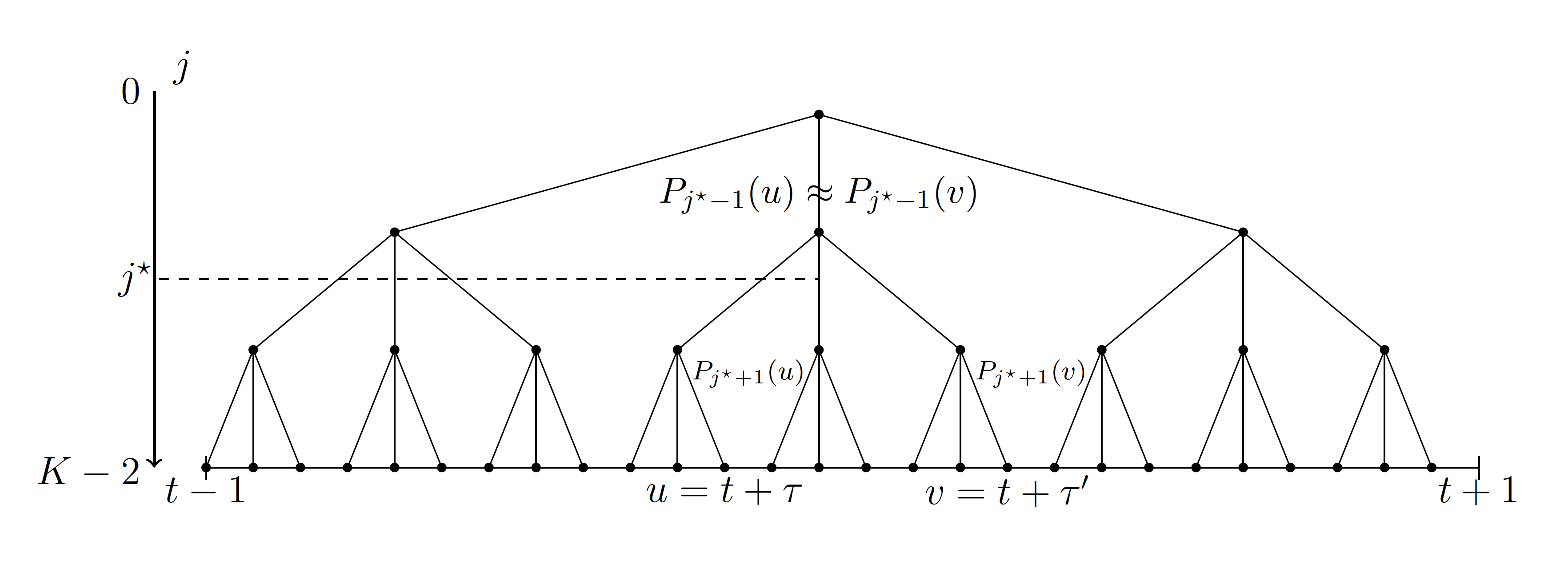
Figure 1. Illustration of the branching random walk approximation of the Dirichlet polynomials $\sum_{j=0}^{K-2}P_{j}$. For two given $\tau,\tau^{\prime}\in[-1,1]$, the increments $P_{j}$ are approximately independent for $j>j^{\star}$ and almost identitical for $j<j^{\star}$ where $j^{\star}={K\frac{-\log|\tau-\tau^{\prime}|}{\log\log T}}$. For the model $\sum_{j=0}^{K-2}\overline{P}_{j}$ this dichotomy holds exactly.

Finally we remark that the ideas involved in the proof of Proposition 3.2 come from many sources. The idea of restricting to an initial subset $B$ of $[T,2T]$ on which an accurate understanding of the distribution of $P_{j}(t)$ can be obtained comes from [Rad11]. The identification of an approximate branching random walk structure within the sum $\sum_{p\leq X}p^{-s}$ was used in [ArgBelHar15] to study the extrema of a random model of the zeta function, and in the subsequent works regarding the large values of characteristic polynomials [ArgBelBou15, ChaMadNaj16, LamPaq16, PaqZei17] and of the zeta function [Naj16]. The original method for studying the extrema of branching processes which we adapt is due to Bramson [Bra78]. More precisely, we use Kistler’s robust $K$-level coarse graining variant from [Kis15], as [ArgBelBou15] did for the related random matrix problem.

Notation. For the rest of the paper, $t$ will denote a uniform random variable on $[T,2T]$. Accordingly, for any event $A_{T}\subset[T,2T]$ and a random variable $X_{T}:[T,2T]\to{\mathbb{C}}$ we write

$$\mathbb{P}(A_{T})=\frac{1}{T}\text{\rm meas}(A_{T}),\qquad\text{and}\qquad\mathbb{E}[X_{T}]=\frac{1}{T}\int_{T}^{2T}X_{T}(t){\rm d}t.$$

We also use the standard $\operatorname{O}$ and $\operatorname{o}$ notations from analytic number theory: thus, $f(T)=\operatorname{O}(g(T))$ means that $|f(T)|/|g(T)|$ is bounded and $f(T)=\operatorname{o}(g(T))$ if $|f(T)|/|g(T)|\to 0$. Sometimes it will be convenient to use the notation $f(T)\ll g(T)$, which means the same as $f(T)=\operatorname{O}(g(T))$. We will encounter some arithmetical functions familiar in number theory. These include: $\omega(n)$ (which counts the number of distinct primes dividing $n$), $\Omega(n)$ (which counts with multiplicity the number of primes dividing $n$), the von Mangoldt function $\Lambda(n)$ (which equals $\log p$ if $n$ is a power of the prime $p$, and equals $0$ otherwise), and the Möbius function $\mu(n)$ (which equals $0$ if $n$ is divisible by the square of a prime, and when $n$ is square-free it equals $(-1)^{\omega(n)}$).

Acknowledgements. The authors thank the referee for useful comments that led to an improvement of the first version of this paper. L.-P. A. is supported by NSF CAREER 1653602, NSF grant DMS-1513441, and a Eugene M. Lang Junior Faculty Research Fellowship. D. B. is grateful for the hospitality of the Courant Institute during visits when part of this work was carried out. P. B. is supported by NSF grant DMS-1513587. M. R. is supported by NSERC DG grant, the CRC program and a Sloan Fellowship. K.S. is partly supported by a grant from the NSF, and a Simons Investigator grant from the Simons Foundation.

2. Proof of the upper bound

The upper bound implicit in our theorem will be a simple consequence of estimates for the second moment of the zeta function and its derivative, together with a Sobolev-type inequality. We begin with the Sobolev inequality, which will also be used elsewhere in the proof. Suppose $f$ (possibly complex valued) is continuously differentiable on $[-1,1]$. For any $u\in[-1,1]$, note that

$$f(u)^{2}=\frac{f(1)^{2}+f(-1)^{2}}{2}+\int_{-1}^{u}f^{\prime}(v)f(v){\rm d}v-\int_{u}^{1}f^{\prime}(v)f(v){\rm d}v,$$

so that using the triangle inequality

(6) $$\max_{u\in[-1,1]}|f(u)|^{2}\leq\frac{|f(1)|^{2}+|f(-1)|^{2}}{2}+\int_{-1}^{1}|f^{\prime}(v)f(v)|{\rm d}v.$$

Proposition 2.1.

Let $V=V(T)$ be any function that tends to infinity as $T\to\infty$. Then

$$\mathbb{P}\Big{(}\max_{|t-u|\leq 1}|\zeta(1/2+\mathrm{i}u)|>V\log T\Big{)}=\operatorname{O}(1/V^{2})=\operatorname{o}(1),$$

where we recall that $t$ is sampled uniformly in the range $[T,2T]$.

Proof.

Chebyshev’s inequality implies that

(7) $$\mathbb{P}\Big{(}\max_{|t-u|\leq 1}|\zeta(1/2+\mathrm{i}u)|>V\log T\Big{)}\leq\frac{1}{V^{2}(\log T)^{2}}\mathbb{E}\left[\max_{|t-u|\leq 1}|\zeta(1/2+\mathrm{i}u)|^{2}\right].$$

Applying (6) with $f(v)=\zeta(1/2+\mathrm{i}t+\mathrm{i}v)$, we obtain

$$\max_{|t-u|\leq 1}|\zeta(1/2+\mathrm{i}u)|^{2}\ll|\zeta(\tfrac{1}{2}+\mathrm{i}(t+1))|^{2}+|\zeta(\tfrac{1}{2}+\mathrm{i}(t-1))|^{2}+\int_{-1}^{1}|\zeta^{\prime}(\tfrac{1}{2}+\mathrm{i}(t+v))\zeta(\tfrac{1}{2}+\mathrm{i}(t+v))|{\rm d}v,$$

so that

$$\mathbb{E}\left[\max_{|t-u|\leq 1}|\zeta(1/2+\mathrm{i}u)|^{2}\right]\ll\frac{1}{T}\int_{T-1}^{2T+1}\Big{(}|\zeta(\tfrac{1}{2}+\mathrm{i}t)|^{2}+|\zeta^{\prime}(\tfrac{1}{2}+\mathrm{i}t)\zeta(\tfrac{1}{2}+\mathrm{i}t)|\Big{)}{\rm d}t.$$

Asymptotics for the second moment of the zeta function and its derivatives are well known (see Chapter VII of [Tit86] and, in the case of the derivative, [Con88]), and these imply the bounds

(8) $$\int_{T-1}^{2T+1}|\zeta(\tfrac{1}{2}+\mathrm{i}t)|^{2}{\rm d}t\ll T\log T,\qquad\text{and}\qquad\int_{T-1}^{2T+1}|\zeta^{\prime}(\tfrac{1}{2}+\mathrm{i}t)|^{2}{\rm d}t\ll T(\log T)^{3}.$$

Using these estimates and Cauchy-Schwarz inequality, we conclude that

$$\mathbb{E}\left[\max_{|t-u|\leq 1}|\zeta(1/2+\mathrm{i}u)|^{2}\right]\ll(\log T)^{2},$$

which, in view of (7), yields the proposition. ∎

3. Plan of the proof of the lower bound

The lower bound of Theorem 1.1 will be proved in two main steps. First, it is shown that the maximum on a short interval of $\log|\zeta|$ is close to the maximum of a Dirichlet polynomial supported on primes slightly to the right of the critical line. This is the content of Proposition 3.1, whose proof builds upon some ideas from [RadSou15]. Second, a lower bound for the maximum of these Dirichlet polynomials on an interval is proved using the robust approach of [Kis15] in Proposition 3.2.

The following notation will be used throughout the remainder of the paper. Motivated by [Kis15], we will fix a large integer $K=K(\varepsilon)$ and divide the primes below

(9) $$X=\exp((\log T)^{1-\frac{1}{K}})$$

into $K-1$ ranges depending on their size, as follows. Take $J_{0}=[2,\exp((\log T)^{\frac{1}{K}})]$, and for $1\leq j\leq K-2$ set

(10) $$J_{j}=(\exp((\log T)^{\frac{j}{K}}),\exp((\log T)^{\frac{j+1}{K}})].$$

For each $0\leq j\leq K-2$, we define the Dirichlet polynomial

(11) $$P_{j}(u)={\rm Re}\sum_{p\in J_{j}}\frac{1}{p^{\sigma_{0}+\mathrm{i}u}},$$

where

(12) $$\sigma_{0}=\frac{1}{2}+\frac{(\log T)^{\frac{3}{2K}}}{\log T}.$$

In the course of the proof, we shall see that if $u$ is chosen uniformly from $[T,2T]$ then $P_{j}(u)$ asymptotically has a Gaussian distribution with mean $0$, and variance $\sim\frac{1}{2}\sum_{p\in J_{j}}1/p^{2\sigma_{0}}$, see for example Lemma 3.4. The prime number theorem enables us to evaluate this variance asymptotically, and we record the relevant estimates for future use. Thus, using the prime number theorem (see for example Theorem 6.9 of [MoVa07]) and partial summation it follows that for some constant $c>0$, and any $\sigma=\frac{1}{2}+\delta$ with $\delta>0$

(13) $$\sum_{x\leq p\leq y}\frac{1}{p^{2\sigma}}=\int_{x}^{y}\frac{1}{u^{2\sigma}\log u}{\rm d}u+\operatorname{O}(e^{-c\sqrt{\log x}})=\log\frac{\log y}{\log x}+\operatorname{O}(\delta\log y+e^{-c\sqrt{\log x}}).$$

Since $(\sigma_{0}-1/2)\times\log(\sup J_{K-3})=(\log T)^{-\frac{1}{2K}}$ it follows that, for all $0\leq j\leq K-3$,

(14) $$\sum_{p\in J_{j}}\frac{1}{p^{2\sigma_{0}}}=\frac{1}{K}\log\log T+\operatorname{O}((\log T)^{-\frac{1}{2K}}),$$

so that the Dirichlet polynomials $P_{j}(u)$ all have roughly the same variance. The last Dirichlet polynomial $P_{K-2}(u)$ has a slightly different variance, with the corresponding sum in (14) being roughly $\frac{1}{2K}\log\log T$.

We are now ready to state the two main propositions from which the lower bound in the theorem will follow.

Proposition 3.1.

Let $\varepsilon>0$ be given, and let $K=K(\varepsilon)$ be a suitably large integer. Then

$$\mathbb{P}\Big{(}\max_{|t-u|\leq 1}\log|\zeta(\tfrac{1}{2}+\mathrm{i}u)| >(1-2\varepsilon)\log\log T\Big{)}$$

$$\geq\mathbb{P}\Big{(}\max_{|t-u|\leq\frac{1}{4}}\sum_{j=1}^{K-3}P_{j}(u)>(1-\varepsilon)\log\log T\Big{)}+\operatorname{o}(1).$$

Note that in Proposition 3.1 we omitted the first and last terms, $P_{0}(u)$ and $P_{K-2}(u)$. The term $P_{K-2}$ is omitted in view of its slightly different variance. The very small primes occurring in $P_{0}$ are omitted so that the Dirichlet sums are not too correlated, a fact essential to the analysis in Section 5.

Proposition 3.2.

Let $K>3$ be a natural number, and $0<\lambda<1$ be a real number. Then

(15) $$\mathbb{P}\Big{(}\max_{|t-u|\leq\frac{1}{4}}\Big{(}\min_{1\leq j\leq K-3}P_{j}(u)\Big{)}>\frac{\lambda}{K}\log\log T\Big{)}=1+\operatorname{o}(1).$$

Proof of Theorem 1.1.

If the event of Proposition 3.2 holds, then

$$\max_{|u-t|\leq\frac{1}{4}}\sum_{j=1}^{K-3}P_{j}(u)>\lambda\Big{(}1-\frac{3}{K}\Big{)}\log\log T.$$

Taking $\lambda$ sufficiently close to $1$, and $K$ large enough, the lower bound of the theorem now follows from Proposition 3.1. ∎

Before proceeding to the proofs of the proposition, we record some simple results on mean values of Dirichlet polynomials which will be repeatedly used below.

Lemma 3.3.

For any complex numbers $a(n)$ and $b(n)$, and $N\leq T$ we have

$$\int_{T}^{2T}\Big{(}\sum_{m\leq N}a(m)m^{-\mathrm{i}t}\Big{)}\Big{(}\sum_{n\leq N}b(n)n^{\mathrm{i}t}\Big{)}{\rm d}t=T\sum_{n\leq N}a(n)b(n)+\operatorname{O}\Big{(}N\log N\sum_{n\leq N}(|a(n)|^{2}+|b(n)|^{2})\Big{)}.$$

Proof.

Expanding out, and performing the integral, gives

$$\sum_{m,n\leq N}a(m)b(n)\int_{T}^{2T}\Big{(}\frac{n}{m}\Big{)}^{\mathrm{i}t}{\rm d}t=T\sum_{n\leq N}a(n)b(n)+\operatorname{O}\Big{(}\sum_{m\neq n\leq N}\frac{|a(m)b(n)|}{|\log(m/n)|}\Big{)}.$$

Using $|a(m)b(n)|\leq|a(m)|^{2}+|b(n)|^{2}$, the remainder term above is

$$\ll\sum_{m\leq N}|a(m)|^{2}\sum_{\begin{subarray}{c}n\leq N\\ n\neq m\end{subarray}}\frac{1}{|\log(m/n)|}+\sum_{n\leq N}|b(n)|^{2}\sum_{\begin{subarray}{c}m\leq N\\ m\neq n\end{subarray}}\frac{1}{|\log(m/n)|}\ll N\log N\sum_{n\leq N}(|a(n)|^{2}+b(n)^{2}),$$

proving the lemma. ∎

The next two lemmas are also standard (for example, see Proposition 3.1 of [Bou10], or Lemma 3 of [Sou09]), and will be useful in comparing moments of Dirichlet polynomials over the primes with the moments of suitable Gaussian distributions.

Lemma 3.4.

Let $x\geq 2$ be a real number, and suppose that for primes $p\leq x$, $a(p)$ and $b(p)$ are complex numbers with $|a(p)|$ and $|b(p)|$ both at most $1$. Then for any natural number $k$ we have

$$\mathbb{E}\Big{[}\Big{(}\frac{1}{2}\sum_{p\leq x}(a(p)p^{-\mathrm{i}t}+b(p)p^{\mathrm{i}t})\Big{)}^{k}\Big{]}=\partial_{z}^{k}\Big{(}\prod_{p\leq x}I_{0}(\sqrt{a(p)b(p)}z)\Big{)}\Big{|}_{z=0}+\operatorname{O}\Big{(}\frac{x^{2k}}{T}\Big{)}$$

where $I_{0}(z)=\sum_{n\geq 0}z^{2n}/(2^{2n}(n!)^{2})$ denotes the Bessel function. In particular, the expression is $\operatorname{O}\left(x^{2k}/T\right)$ for odd $k$.

Proof.

Given $n$ with prime factorization $n=p_{1}^{\alpha_{1}}\cdots p_{r}^{\alpha_{r}}$, we set $a(n)=\prod_{j}a(p_{j})^{\alpha_{j}}$, and $b(n)=\prod_{j}b(p_{j})^{\alpha_{j}}$, with the understanding that $a(n)$ and $b(n)$ are $0$ if $n$ has a prime factor larger than $x$. We also define temporarily the multiplicative function $g$ given by $g(p^{\alpha})=1/\alpha!$ on prime powers $p^{\alpha}$. With this notation, we may expand (recall $\Omega(n)$ counts with multiplicity the number of prime factors of $n$)

$$\Big{(}\frac{1}{2}\sum_{p\leq x} (a(p)p^{-\mathrm{i}t}+b(p)p^{\mathrm{i}t})\Big{)}^{k}$$

$$=\frac{1}{2^{k}}\sum_{\ell=0}^{k}\binom{k}{\ell}\Big{(}\ell!\sum_{\Omega(m)=\ell}a(m)g(m)m^{-\mathrm{i}t}\Big{)}\Big{(}(k-\ell)!\sum_{\Omega(n)=k-\ell}b(n)g(n)n^{\mathrm{i}t}\Big{)}.$$

Now we appeal to Lemma 3.3 to evaluate the expectation of the above quantity. The remainder terms that arise are

$$\ll\frac{x^{k}\log(x^{k})}{T}\frac{1}{2^{k}}\sum_{\ell=0}^{k}\binom{k}{\ell}\Big{(}\pi(x)^{\ell}+\pi(x)^{k-\ell}\Big{)}\ll\frac{x^{2k}}{T},$$

where $\pi(x)\sim x/\log x$ denotes the number of primes below $x$.

Now let us consider the main terms arising from Lemma 3.3. These arise from the diagonal terms $m=n$, so that $\ell=\Omega(m)=k-\ell=\Omega(n)$. Thus when $k$ is odd there is no main term, and when $k$ is even, we get a main term contribution of

$$\frac{1}{2^{k}}k!\sum_{\Omega(n)=k/2}a(n)b(n)g(n)^{2}.$$

This is $k!$ times the coefficient of $z^{k}$ in

$$\sum_{n}a(n)b(n)g(n)^{2}(z^{2}/4)^{\Omega(n)}=\prod_{p\leq x}I_{0}(\sqrt{a(p)b(p)}z),$$

since the terms appearing on the left side are multiplicative. ∎

The last lemma gives a useful bound for the $2k$-th moment of Dirichlet polynomials supported on primes; it may be deduced by a variant of our argument for the previous lemma, or see Lemma 3 of [Sou09].

Lemma 3.5.

Let $x\geq 2$ be a real number, and suppose $\sigma\geq\frac{1}{2}$. Let $k$ be a natural number such that $x^{k}\leq T(\log T)^{-1}$. Then, for any sequence of complex numbers $a(p)$ defined on the primes $p$ below $x$,

$$\frac{1}{T}\int_{T}^{2T}\Big{|}\sum_{p\leq x}\frac{a(p)}{p^{\sigma+\mathrm{i}t}}\Big{|}^{2k}{\rm d}t\ll k!\Big{(}\sum_{p\leq x}\frac{|a(p)|^{2}}{p^{2\sigma}}\Big{)}^{k}.$$

4. Proof of Proposition 3.1

4.1. Step 1.

We divide the proof of the proposition into three parts, the first of which bounds the maximum of the zeta function over intervals of the critical line in terms of the maximum over intervals lying slightly to the right of the critical line.

Lemma 4.1.

Let $\varepsilon>0$ be given, and suppose $\tfrac{1}{2}\leq\sigma\leq\frac{1}{2}+(\log T)^{-1/2-\varepsilon}$. Then, for any real number $V\geq 2$,

$$\mathbb{P}\Big{(}\max_{|t-u|\leq 1}|\zeta\left(1/2+\mathrm{i}u\right)|>V\Big{)}\geq\mathbb{P}\Big{(}\max_{|t-u|\leq\frac{1}{4}}|\zeta(\sigma+\mathrm{i}u)|>2V\Big{)}+\operatorname{o}(1).$$

Proof.

From Theorem 4.11 of [Tit86] we recall that for $\sigma\geq\tfrac{1}{2}$

(16) $$\zeta(\sigma+\mathrm{i}t)=\sum_{n\leq T}\frac{1}{n^{\sigma+\mathrm{i}t}}+\operatorname{O}(T^{-\frac{1}{2}}).$$

Using knowledge of the Fourier transform of the function $e^{-|x|}$, we may write

$$\frac{1}{n^{\sigma-\frac{1}{2}}}=\frac{1}{\pi}\int_{-\infty}^{\infty}n^{-iv}\frac{(\sigma-1/2)}{(\sigma-1/2)^{2}+v^{2}}{\rm d}v=\frac{1}{\pi}\int_{-T/2}^{T/2}n^{-iv}\frac{(\sigma-1/2)}{(\sigma-1/2)^{2}+v^{2}}{\rm d}v+O(T^{-1}).$$

Thus we see that

(17) $$\zeta(\sigma+\mathrm{i}t)=\frac{1}{\pi}\int_{-T/2}^{T/2}\zeta\left(1/2+\mathrm{i}(t+v)\right)\frac{\sigma-1/2}{(\sigma-1/2)^{2}+v^{2}}{\rm d}v+O(T^{-\frac{1}{2}}).$$

Consider $t\in[T,2T]$ such that $\max_{|v|\leq\frac{1}{4}}|\zeta\left(\sigma+\mathrm{i}(t+v)\right)|>2V$ but $\max_{|v|<1}|\zeta(1/2+\mathrm{i}(t+v))|\leq V$; we must show that the measure of the set of such points $t$ is $\operatorname{o}(T)$. If $t$ is such a point, then denote by $v^{\star}=v^{\star}(t)$ the $v\in[-\frac{1}{4},\frac{1}{4}]$ where the maximum of $|\zeta(\sigma+\mathrm{i}(t+v))|$ is attained. Applying (17) to the point $\sigma+\mathrm{i}(t+v^{\star})$ we obtain

$$2V<|\zeta(\sigma+\mathrm{i}(t+v^{\star}))|\leq\frac{1}{\pi}\int_{-T/2}^{T/2}|\zeta\left(1/2+\mathrm{i}(t+v^{\star}+v)\right)|\frac{(\sigma-1/2)}{(\sigma-1/2)^{2}+v^{2}}{\rm d}v+\operatorname{O}(T^{-\frac{1}{2}}).$$

Since $|\zeta(1/2+iu)|\leq V$ for $|t-u|\leq 1$ (by assumption), the portion of the integral above with $|v|\leq\frac{3}{4}$ is less than $V$. Therefore it follows that

$$V+\operatorname{O}(T^{-\frac{1}{2}})\leq\frac{1}{\pi}\int_{\frac{3}{4}\leq|v|\leq\frac{T}{2}}|\zeta\left(1/2+\mathrm{i}(t+v^{\star}+v)\right)|\frac{(\sigma-1/2)}{(\sigma-1/2)^{2}+v^{2}}{\rm d}v.$$

Using the Cauchy-Schwarz inequality, we deduce that for such $t$,

$$\Big{(}\frac{V}{(\sigma-1/2)}\Big{)}^{2}\ll\Big{(}\int_{\frac{3}{4}\leq|v|\leq\frac{T}{2}}|\zeta(1/2+\mathrm{i}(t+v^{\star}+v))|\frac{{\rm d}v}{v^{2}}\Big{)}^{2}\ll\int_{\frac{1}{2}\leq|v|\leq\frac{T}{2}}|\zeta(1/2+\mathrm{i}(t+v))|^{2}\frac{{\rm d}v}{v^{2}}.$$

Therefore, by Chebyshev’s inequality, the measure of the set of such points $t\in[T,2T]$ is

$$\ll\Big{(}\frac{(\sigma-1/2)}{V}\Big{)}^{2}\int_{T}^{2T}\int_{\frac{1}{2}\leq|v|\leq\frac{T}{2}}|\zeta(1/2+\mathrm{i}(t+v))|^{2}\frac{{\rm d}v}{v^{2}}{\rm d}t\ll\Big{(}\frac{(\sigma-1/2)}{V}\Big{)}^{2}\int_{T/2}^{5T/2}|\zeta(1/2+\mathrm{i}t)|^{2}{\rm d}t,$$

which, by (8) and the assumption on $\sigma$, is

$$\ll(\sigma-1/2)^{2}T\log T=\operatorname{o}(T).$$

∎

4.2. Step 2.

The second part of the attack will consist of showing that on the $\sigma_{0}$ line, one can typically invert $\zeta(\sigma_{0}+it)$ and replace it by a suitable Dirichlet polynomial. We define

(18) $$M(s)=\sum_{n}\frac{\mu(n)a(n)}{n^{s}},$$

where the factor $a(n)$ equals $1$ if all primes factors of $n$ are smaller than $X$ and $\Omega(n)\leq 100K\log\log T=:\nu$, and $a(n)=0$ otherwise. Recall that $\mu$ denotes the Möbius function, $\Omega(n)$ counts the number of prime factors of $n$ (with multiplicity), and $X$ was defined in (9). The choice of the Dirichlet polynomial $M$ is motivated by work in [RadSou15], which in turn is motivated by classical ideas on mollifying the zeta function. Adapting the proof of Proposition 3 in [RadSou15], we first establish the following preliminary result.

Lemma 4.2.

With the above notation

$$\int_{T}^{2T}|\zeta(\sigma_{0}+\mathrm{i}t)M(\sigma_{0}+\mathrm{i}t)-1|^{2}{\rm d}t=\operatorname{O}\Big{(}\frac{T}{(\log T)^{100}}\Big{)}.$$

Proof.

From its definition, $a(n)=0$ unless $n\leq X^{\nu}<T^{\varepsilon}$ ($\varepsilon>0$ is a fixed arbitrarily small constant), and therefore estimating trivially one has $M(\sigma_{0}+\mathrm{i}t)\ll T^{\varepsilon}$. Combining this with (16), we see that

$$\int_{T}^{2T}\zeta(\sigma_{0}+\mathrm{i}t)M(\sigma_{0}+\mathrm{i}t){\rm d}t=\int_{T}^{2T}\sum_{n\leq T}\frac{1}{n^{\sigma_{0}+\mathrm{i}t}}\sum_{m}\frac{\mu(m)a(m)}{m^{\sigma_{0}+\mathrm{i}t}}{\rm d}t+\operatorname{O}(T^{\frac{1}{2}+\varepsilon}).$$

Carrying out the integral over $t$, this is

$$T+\operatorname{O}\Big{(}\sum_{\begin{subarray}{c}n\leq T,m\leq X^{\nu}\\ {mn>1}\end{subarray}}\frac{1}{(mn)^{\sigma_{0}}}\Big{)}+\operatorname{O}(T^{\frac{1}{2}+\varepsilon})=T+\operatorname{O}(T^{\frac{1}{2}+\varepsilon}).$$

Thus, expanding out the square in the desired integral, we see that it equals

(19) $$\int_{T}^{2T}|\zeta(\sigma_{0}+\mathrm{i}t)M(\sigma_{0}+\mathrm{i}t)|^{2}{\rm d}t-T+\operatorname{O}(T^{\frac{1}{2}+\varepsilon}).$$

To estimate the second moment in (19), we invoke Lemma 4 for [RadSou15]: for any $h,k\leq T$ and $1/2<\sigma\leq 1$, we have

$$\int_{T}^{2T}\Big{(}\frac{h}{k}\Big{)}^{\mathrm{i}t}\left|\zeta\left(\sigma+\mathrm{i}t\right)\right|^{2}{\rm d}t =\int_{T}^{2T}\Big{(}\zeta(2\sigma)\Big{(}\frac{(h,k)^{2}}{hk}\Big{)}^{\sigma}+\Big{(}\frac{t}{2\pi}\Big{)}^{1-2\sigma}\zeta(2-2\sigma)\Big{(}\frac{(h,k)^{2}}{hk}\Big{)}^{1-\sigma}\Big{)}{\rm d}t$$

(20) $$\hskip 72.26999pt+\operatorname{O}(T^{1-\sigma+\varepsilon}\min(h,k)).$$

Using this result, we may write

$$\int_{T}^{2T}|\zeta(\sigma_{0}+\mathrm{i}t)M(\sigma_{0}+\mathrm{i}t)|^{2}{\rm d}t =\sum_{h,k}\frac{\mu(h)a(h)\mu(k)a(k)}{h^{\sigma_{0}}k^{\sigma_{0}}}\int_{T}^{2T}\Big{(}\frac{h}{k}\Big{)}^{\mathrm{i}t}|\zeta(\sigma_{0}+\mathrm{i}t)|^{2}{\rm d}t$$

(21) $$=S_{1}+S_{2}+E,$$

say, with

(22) $$S_{1}=T\zeta(2\sigma_{0})\sum_{h,k}\frac{\mu(h)a(h)\mu(k)a(k)}{(hk)^{\sigma_{0}}}\Big{(}\frac{(h,k)^{2}}{hk}\Big{)}^{\sigma_{0}},$$

(23) $$S_{2}=\zeta(2-2\sigma_{0})\Big{(}\int_{T}^{2T}\Big{(}\frac{t}{2\pi}\Big{)}^{1-2\sigma_{0}}{\rm d}t\Big{)}\sum_{h,k}\frac{\mu(h)a(h)\mu(k)a(k)}{(hk)^{\sigma_{0}}}\Big{(}\frac{(h,k)^{2}}{hk}\Big{)}^{1-\sigma_{0}},$$

and

(24) $$E=\operatorname{O}\Big{(}T^{\frac{1}{2}+\varepsilon}\sum_{h,k\leq T^{\varepsilon}}\frac{1}{(hk)^{\sigma_{0}}}\min(h,k)\Big{)}=\operatorname{O}(T^{\frac{1}{2}+\varepsilon}).$$

Now consider the quantity $S_{1}$. Here the sum is over all $h$ and $k$ whose prime factors are below $X$, and with $\Omega(h)$ and $\Omega(k)$ below $\nu$. If we retain the first condition, but drop the second condition, then the contribution to $S_{1}$ would be (upon considering whether a prime $p$ divides neither $h$ nor $k$, or divides exactly one of $h$ or $k$, or divides both $h$ and $k$)

$$T\zeta(2\sigma_{0})\sum_{\begin{subarray}{c}h,k\\ p|hk\implies p\leq X\end{subarray}}\frac{\mu(h)\mu(k)}{(hk)^{\sigma_{0}}}\Big{(}\frac{(h,k)^{2}}{hk}\Big{)}^{\sigma_{0}} =T\zeta(2\sigma_{0})\prod_{p\leq X}\Big{(}1-\frac{1}{p^{2\sigma_{0}}}-\frac{1}{p^{2\sigma_{0}}}+\frac{1}{p^{2\sigma_{0}}}\Big{)}$$

(25) $$=T\zeta(2\sigma_{0})\prod_{p\leq X}\Big{(}1-\frac{1}{p^{2\sigma_{0}}}\Big{)}.$$

The difference between $S_{1}$ and (4.2) comes from the terms with either $\Omega(h)$ or $\Omega(k)$ being larger than $\nu$, and these terms give a contribution bounded by (assuming that $\Omega(h)$ is larger than $\nu$)

$$\ll T\zeta(2\sigma_{0})\sum_{\begin{subarray}{c}h,k\\ \Omega(h)>\nu\\ p|hk\implies p\leq X\end{subarray}}\frac{|\mu(h)\mu(k)|}{(hk)^{\sigma_{0}}}\Big{(}\frac{(h,k)^{2}}{hk}\Big{)}^{\sigma_{0}}$$

$$\ll T\zeta(2\sigma_{0})e^{-\nu}\sum_{\begin{subarray}{c}h,k\\ p|hk\implies p\leq X\end{subarray}}\frac{|\mu(h)\mu(k)|}{(hk)^{\sigma_{0}}}\Big{(}\frac{(h,k)^{2}}{hk}\Big{)}^{\sigma_{0}}e^{\Omega(h)},$$

since $e^{\Omega(h)-\nu}\geq 1$ when $\Omega(h)\geq\nu$, and is non-negative for other terms. The sum over $h$ and $k$ may now be expressed as a product over the primes below $X$, yielding

$$T\zeta(2\sigma_{0})e^{-\nu}\prod_{p\leq X}\Big{(}1+\frac{e}{p^{2\sigma_{0}}}+\frac{1}{p^{2\sigma_{0}}}+\frac{e}{p^{2\sigma_{0}}}\Big{)}\ll T(\log T)e^{-\nu}\prod_{p\leq X}\Big{(}1+\frac{7}{p}\Big{)}\ll\frac{T}{(\log T)^{100}}.$$

Thus

$$S_{1}=T\zeta(2\sigma_{0})\prod_{p\leq X}\Big{(}1-\frac{1}{p^{2\sigma_{0}}}\Big{)}+O\Big{(}\frac{T}{(\log T)^{100}}\Big{)}=T\prod_{p>X}\Big{(}1-\frac{1}{p^{2\sigma_{0}}}\Big{)}^{-1}+\operatorname{O}\Big{(}\frac{T}{(\log T)^{100}}\Big{)}.$$

Recalling the definitions of $\sigma_{0}$ and $X$, we find $(\sigma_{0}-1/2)\log X=(\log T)^{\frac{1}{2K}}$, and so

$$\sum_{p>X}\log\Big{(}1-\frac{1}{p^{2\sigma_{0}}}\Big{)}^{-1}\ll\sum_{p>X}\frac{1}{p^{2\sigma_{0}}}\ll X^{-(\sigma_{0}-1/2)}\sum_{p>X}\frac{1}{p^{\sigma_{0}+1/2}}\ll(\log T)^{-100},$$

which enables us to conclude that $S_{1}=T+O(T/(\log T)^{100})$.

Arguing similarly, we see that

$$S_{2}\sim\zeta(2-2\sigma_{0})\Big{(}\int_{T}^{2T}\Big{(}\frac{t}{2\pi}\Big{)}^{1-2\sigma_{0}}{\rm d}t\Big{)}\prod_{p\leq X}\Big{(}1-\frac{2}{p}+\frac{1}{p^{2\sigma_{0}}}\Big{)}\ll T^{2-2\sigma_{0}}\log T\ll\frac{T}{(\log T)^{100}}.$$

Inserting the evaluation of $S_{1}$ with the estimates for $S_{2}$ and $E$ into (4.2), and then into (19), we obtain the lemma. ∎

Lemma 4.2 ensures that for most $t$ one has $\zeta(\sigma_{0}+\mathrm{i}t)M(\sigma_{0}+\mathrm{i}t)\approx 1$, and we next refine this to ensure that for most $t$ one has $\zeta(\sigma_{0}+\mathrm{i}u)M(\sigma_{0}+\mathrm{i}u)\approx 1$ for all $u$ with $|u-t|\leq 1$.

Lemma 4.3.

For any $\varepsilon>0$, we have

$$\mathbb{P}\Big{(}\max_{|t-u|\leq 1}\left|M(\sigma_{0}+\mathrm{i}u)\zeta(\sigma_{0}+\mathrm{i}u)-1\right|>\varepsilon\Big{)}=\operatorname{o}(1).$$

Proof.

We deduce this from Lemma 4.2 and a Sobolev inequality argument. Note that by (6), we have

$$\max_{|t-u|\leq 1}|\zeta M(\sigma_{0}+\mathrm{i}u)-1|^{2} \ll|\zeta M(\sigma_{0}+\mathrm{i}(t+1))-1|^{2}+|\zeta M(\sigma_{0}+\mathrm{i}(t-1))-1|^{2}$$

$$+\int_{t-1}^{t+1}|\zeta M(\sigma_{0}+\mathrm{i}v)-1||(\zeta^{\prime}M+\zeta M^{\prime})(\sigma_{0}+\mathrm{i}v)|{\rm d}v.$$

Ignoring the end cases $t\in[T,T+1]$ or $t\in[2T-1,2T]$, by Chebyshev’s inequality the probability we want to bound is (using the above estimate)

$$\ll\frac{1}{T}+\frac{1}{\varepsilon^{2}T}\int_{T}^{2T}\big{(}|\zeta M(\sigma_{0}+\mathrm{i}(t+1))-1|^{2}+|\zeta M(\sigma_{0}+\mathrm{i}t)-1||(\zeta^{\prime}M+\zeta M^{\prime})(\sigma_{0}+\mathrm{i}t)|\big{)}{\rm d}t.$$

Applying the Cauchy-Schwarz inequality and Lemma 4.2 this is

$$\ll\frac{1}{\varepsilon^{2}(\log T)^{100}}+\frac{1}{\varepsilon^{2}(\log T)^{50}}\Big{(}\frac{1}{T}\int_{T}^{2T}\big{(}|\zeta^{\prime}M|^{2}+|\zeta M^{\prime}|^{2}\big{)}(\sigma_{0}+\mathrm{i}t){\rm d}t\Big{)}^{\frac{1}{2}}.$$

We can bound the last integral above by adapting the argument in [RadSou15], as we did in the proof of Lemma 4.2. Or, we can finesse the issue by using the Cauchy-Schwarz inequality once again to bound that term by

$$\ll\Big{(}\frac{1}{T}\int_{T}^{2T}(|\zeta|^{4}+|\zeta^{\prime}|^{4})(\sigma_{0}+\mathrm{i}t){\rm d}t\Big{)}^{\frac{1}{4}}\Big{(}\frac{1}{T}\int_{T}^{2T}(|M|^{4}+|M^{\prime}|^{4})(\sigma_{0}+\mathrm{i}t){\rm d}t\Big{)}^{\frac{1}{4}},$$

and then use the work of Conrey [Con88] to bound the first factor by $\ll(\log T)^{2}$, and apply Lemma 3.3 to bound the second term by $\ll(\log T)^{2}$. This completes the proof, with a lot of room to spare. ∎

4.3. Step 3.

The last stage in our proof involves connecting $\log|M(\sigma_{0}+\mathrm{i}t)|$ (for most $t$) with (close relatives) of the Dirichlet polynomials over primes $P_{j}(t)$. For $0\leq j\leq K-2$, define the Dirichlet polynomials

(26) $$\mathcal{P}_{j}(t)=\sum_{n\in J_{j}}\frac{\Lambda(n)}{n^{\sigma_{0}+\mathrm{i}t}\log n},\qquad\text{and}\qquad{\widetilde{P}}_{j}(t)=\sum_{p\in J_{j}}\frac{1}{p^{\sigma_{0}+\mathrm{i}t}}.$$

Note that $P_{j}(t)$ is simply the real part of ${\widetilde{P}}_{j}(t)$, and the difference between ${\mathcal{P}}_{j}$ and ${\widetilde{P}}_{j}$ is only in the prime powers; estimating the contribution of prime cubes and larger powers trivially we see that

(27) $$Q(t)=\sum_{j=0}^{K-2}({\mathcal{P}}_{j}(t)-{\widetilde{P}}_{j}(t))=\frac{1}{2}\sum_{p\leq\sqrt{X}}\frac{1}{p^{2\sigma_{0}+2\mathrm{i}t}}+\operatorname{O}(1).$$

Our goal is to show that for most $t$ one has $\max_{|t-u|\leq 1}|M(\sigma_{0}+\mathrm{i}u)-\exp(-\sum_{j=0}^{K-2}{\mathcal{P}}_{j}(u))|$ is small, and we begin with the following preliminary lemma.

Lemma 4.4.

With notation as above,

$$\mathbb{P}\Big{(}\max_{|t-u|\leq 1}|Q(u)|\geq\log\log\log T\Big{)}=\operatorname{o}(1),$$

and

$$\mathbb{P}\Big{(}\max_{|t-u|\leq 1}\max_{0\leq j\leq K-2}|{\widetilde{P}}_{j}(u)|\geq{10}K^{-\frac{1}{2}}\log\log T\Big{)}=\operatorname{o}(1).$$

Proof.

The Sobolev inequality (6) gives

$$\max_{|t-u|\leq 1}|Q(u)|^{2}\ll|Q(t+1)|^{2}+|Q(t-1)|^{2}+\int_{-1}^{1}|Q(t+v)Q^{\prime}(t+v)|{\rm d}v,$$

so that, using Chebyshev’s inequality and the Cauchy-Schwarz inequality,

$$(\log\log\log T)^{2}\mathbb{P}\Big{(}\max_{|t-u|\leq 1}|Q(u)|\geq\log\log\log T\Big{)}\ll\frac{1}{T}+\mathbb{E}[|Q(t)|^{2}]+\Big{(}\mathbb{E}[|Q(t)|^{2}]\mathbb{E}[|Q^{\prime}(t)|^{2}]\Big{)}^{\frac{1}{2}}.$$

A quick calculation with Lemma 3.3 shows that $\mathbb{E}[|Q(t)|^{2}]$ and $\mathbb{E}[|Q^{\prime}(t)|^{2}]$ are $\operatorname{O}(1)$, which yields the first assertion of the lemma.

Let $\ell$ denote a natural number to be chosen later. Applying (6) to the function ${\widetilde{P}}_{j}(t)^{\ell}$, we obtain

$$\max_{|t-u|\leq 1}|{\widetilde{P}}_{j}(u)|^{2\ell}\ll|{\widetilde{P}}_{j}(t-1)|^{2\ell}+|{\widetilde{P}}_{j}(t+1)|^{2\ell}+\ell\int_{t-1}^{t+1}|{\widetilde{P}}_{j}(v)|^{2\ell-1}|{\widetilde{P}}_{j}^{\prime}(v)|{\rm d}v.$$

Combining this with Chebyshev’s inequality and the Cauchy-Schwarz inequality, we may bound $\mathbb{P}(\max_{|u-t|\leq 1}|{\widetilde{P}}_{j}(u)|\geq 10K^{-\frac{1}{2}}\log\log T)$ by

(28) $$\ll\frac{1}{T}+(10K^{-\frac{1}{2}}\log\log T)^{-2\ell}\Big{(}\mathbb{E}[|{\widetilde{P}}_{j}(t)|^{2\ell}]+\ell\Big{(}\mathbb{E}[|{\widetilde{P}}_{j}(t)|^{4\ell-2}]\mathbb{E}[|{\widetilde{P}}_{j}^{\prime}(t)|^{2}]\Big{)}^{\frac{1}{2}}\Big{)}.$$

Now an application of Lemma 3.3 shows that

$$\mathbb{E}[|{\widetilde{P}}_{j}^{\prime}(t)|^{2}]\ll\sum_{p\in{J_{j}}}\frac{(\log p)^{2}}{p^{2\sigma_{0}}}\ll(\log T)^{2},$$

and an application of Lemma 3.5 gives

$$\mathbb{E}[|{\widetilde{P}}_{j}(t)|^{4\ell-2}]\ll(2\ell-1)!\Big{(}\sum_{p\in J_{j}}\frac{1}{p^{2\sigma_{0}}}\Big{)}^{2\ell-1}\ll(\ell K^{-1}\log\log T)^{2\ell-1}.$$

Upon choosing $\ell=[10\log\log T]$, we conclude from this and (28) that

$$\mathbb{P}\left(\max_{|u-t|\leq 1}|{\widetilde{P}}_{j}(u)|\geq 10\log\log T\right)\ll(\log T)\Big{(}\frac{\ell K^{-1}\log\log T}{100K^{-1}(\log\log T)^{2}}\Big{)}^{\ell}\ll(\log T)^{-10}.$$

Using a union bound for each $0\leq j\leq K-2$, we obtain a stronger form of the claimed lemma. ∎

We are ready to connect $M(\sigma_{0}+\mathrm{i}t)$ with $\exp(-\sum_{j=0}^{K-3}{\mathcal{P}}_{j}(t))$ for most values of $t$.

Lemma 4.5.

We have

$$\mathbb{P}\Big{(}\max_{|t-u|\leq 1}\Big{|}M(\sigma_{0}+\mathrm{i}u)-\exp\Big{(}-\sum_{j=0}^{K-2}\mathcal{P}_{j}(u)\Big{)}\Big{|}>(\log T)^{-2}\Big{)}=\operatorname{o}(1)\ .$$

Proof.

Recalling that $\nu=100K\log\log T$, we define the truncated exponential

(29) $$\mathcal{M}(t)=\sum_{k\leq\nu}\frac{(-1)^{k}}{k!}\Big{(}\sum_{j=0}^{K-2}\mathcal{P}_{j}(t)\Big{)}^{k}.$$

By Lemma 4.4, we know that with probability $1+\operatorname{o}(1)$ (in $t$) one has

$$\max_{|t-u|\leq 1}\Big{|}\sum_{j=0}^{K-2}{\mathcal{P}}_{j}(u)\Big{|}\leq\max_{|t-u|\leq 1}\Big{(}|Q(u)|+\sum_{j=0}^{K-2}|{\widetilde{P}}_{j}(u)|\Big{)}\leq 10K\log\log T.$$

For such a typical $t$, one has

$$\max_{|u-t|\leq 1}\Big{|}{\mathcal{M}}(u)-\exp\Big{(}-\sum_{j=0}^{K-2}{\mathcal{P}}_{j}(u)\Big{)}\Big{|}\leq\sum_{k>\nu}\frac{1}{k!}(10K\log\log T)^{k}\ll(\log T)^{-100}.$$

Therefore, the lemma would follow once we establish that

(30) $$\mathbb{P}\Big{(}\max_{|t-u|\leq 1}\left|M(\sigma_{0}+\mathrm{i}u)-\mathcal{M}(u)\right|>(\log T)^{-3}\Big{)}=\operatorname{o}(1)\ .$$

The quantities $M(\sigma_{0}+\mathrm{i}u)$ and ${\mathcal{M}}(u)$ are almost identical, differing only in a small number of terms. More precisely, if we write ${\mathcal{M}}(u)=\sum_{n}b(n)n^{-\sigma_{0}-\mathrm{i}u}$, then one may check that (i) $|b(n)|\leq 1$ always, (ii) $b(n)=0$ unless $n\leq X^{\nu}$ is composed only of primes below $X$, and (iii) $b(n)=\mu(n)a(n)$ unless $\Omega(n)>\nu$, or if there is a prime $p\leq X$ such that $p^{k}|n$ with $p^{k}>X$. Therefore, an application of Lemma 3.3 gives

$$\mathbb{E}[|M(\sigma_{0}+\mathrm{i}t)-{\mathcal{M}}(t)|^{2}]\ll\sum_{\begin{subarray}{c}p|n\implies p\leq X\\ \Omega(n)>\nu\end{subarray}}\frac{1}{n}+\Big{(}\sum_{\begin{subarray}{c}p\leq X\\ p^{k}>X\end{subarray}}\frac{1}{p^{k}}\Big{)}\Big{(}\sum_{p|n\implies p\leq X}\frac{1}{n}\Big{)}.$$

The second term above is $\ll(\log X)/\sqrt{X}\ll(\log T)^{-100}$. Since $e^{(\Omega(n)-\nu)/2}$ is $\geq 1$ when $\Omega(n)>\nu$, and is positive for all other $n$, we may bound the first term above by

$$e^{-\nu/2}\sum_{p|n\implies p\leq X}\frac{e^{\Omega(n)/2}}{n}\ll(\log T)^{-50K}\prod_{p\leq X}\Big{(}1+\sum_{j=1}^{\infty}\frac{e^{j/2}}{p^{j}}\Big{)}\ll(\log T)^{-50}.$$

We conclude that

$$\mathbb{E}[|M(\sigma_{0}+\mathrm{i}t)-{\mathcal{M}}(t)|^{2}]\ll(\log T)^{-50}.$$

A simple application of Lemma 3.3 also shows that $\mathbb{E}[|M^{\prime}(\sigma_{0}+\mathrm{i}t)|^{2}]$ and $\mathbb{E}[|{\mathcal{M}}^{\prime}(t)|^{2}]$ are $\ll(\log T)^{3}$. The estimate (30) follows as in Lemmas 4.4 and 4.5 by a successive application of the Sobolev inequality (6), Chebyshev’s inequality and the Cauchy-Schwarz inequality, proving the lemma. ∎

4.4. Finishing the proof of Proposition 3.1

It is now simply a matter of assembling the results established above. From Lemma 4.1 we obtain for any $V\geq 2$

$$\mathbb{P}(\max_{|t-u|\leq 1}|\zeta(\tfrac{1}{2}+\mathrm{i}u)|\geq V)\geq\mathbb{P}(\max_{|t-u|\leq\frac{1}{4}}|\zeta(\sigma_{0}+\mathrm{i}u)|\geq 2V)+\operatorname{o}(1).$$

By Lemma 4.3 this quantity is

$$\geq\mathbb{P}(\max_{|t-u|\leq\frac{1}{4}}|M(\sigma_{0}+\mathrm{i}u)|^{-1}\geq 4V)+\operatorname{o}(1),$$

and by Lemma 4.5 the above is

$$\geq\mathbb{P}\Big{(}\max_{|t-u|\leq\frac{1}{4}}\sum_{j=0}^{K-2}\text{Re }{\mathcal{P}}_{j}(u)\geq\log(8V)\Big{)}+\operatorname{o}(1).$$

Invoking Lemma 4.4, we may replace Re${\mathcal{P}}_{j}(u)$ by $P_{j}(u)$ with negligible error, and also discard the terms with $j=0$ and $j=K-2$: thus, the quantity above is

$$\geq\mathbb{P}\Big{(}\max_{|t-u|\leq\frac{1}{4}}\sum_{j=1}^{K-3}P_{j}(u)\geq\log(8V)+\log\log\log T+20K^{-\frac{1}{2}}\log\log T\Big{)}+\operatorname{o}(1).$$

Taking $V=(\log T)^{1-2\varepsilon}$, the proposition follows.

5. Proof of Proposition 3.2

The proof of the proposition is based on large deviation estimates for $P_{j}(u)$ (defined in (11) and (12)), see Propositions 5.4 and 5.5. In Section 5.1, we estimate the Fourier-Laplace transform of $P_{j}(u)$ in a wide range, using Lemma 3.4 to evaluate moments of Dirichlet polynomials. The large deviation estimates are then derived by inverting the Fourier-Laplace transforms, in Section 5.2. The proof of Proposition 3.2 is completed in Section 5.3.

5.1. Fourier-Laplace Transform of Dirichlet Polynomials

The first step is to show that the moments of sums of $P_{j}$’s are very close to Gaussian moments.

Proposition 5.1.

For $1\leq j\leq K-3$ let $\xi_{j}$ and $\xi_{j}^{\prime}$ denote complex numbers with $|\xi_{j}|$, $|\xi_{j}^{\prime}|\leq(\log T)^{\frac{1}{16K}}$. Let $\tau$ denote a real number with $|\tau|\leq 1$. If $n\leq(\log T)^{\frac{1}{2K}}$ is odd then

$$\mathbb{E}\Big{[}\Big{(}\sum_{j=1}^{K-3}\{\xi_{j}P_{j}(t)+\xi_{j}^{\prime}P_{j}(t+\tau)\}\Big{)}^{n}\Big{]}=\operatorname{O}(\exp(-(\log T)^{\frac{1}{3K}})).$$

If $n\leq(\log T)^{\frac{1}{2K}}$ is even,

$$\mathbb{E}\Big{[}\Big{(}\sum_{j=1}^{K-3}\{\xi_{j}P_{j}(t)+\xi_{j}^{\prime}P_{j}(t+\tau)\}\Big{)}^{n}\Big{]} =\frac{n!}{2^{n/2}(n/2)!}\ \Big{(}\sum_{j=1}^{K-3}\{s_{j}^{2}(\xi_{j}^{2}+{\xi^{\prime}}^{2}_{j})+2\rho_{j}(\tau)\xi_{j}\xi^{\prime}_{j}\}\Big{)}^{n/2}$$

(31) $$\hskip 72.26999pt+\operatorname{O}(\exp(-(\log T)^{\frac{1}{3K}})),$$

where

(32) $$s_{j}^{2}=\frac{1}{2}\sum_{p\in J_{j}}p^{-2\sigma_{0}}\mbox{ and }\rho_{j}(\tau)=\frac{1}{2}\sum_{p\in J_{j}}p^{-2\sigma_{0}}\cos(\tau\log p).$$

Ignoring the remainder term, the moments evaluated in (5.1) correspond exactly with what would happen if $P_{j}(t)$ and $P_{j}(t+\tau)$ were jointly Gaussian with variance $s_{j}^{2}$ and covariance $\rho_{j}(\tau)$, and with $P_{j}(t)$ and $P_{j}(t+\tau)$ being uncorrelated with $P_{k}(t)$ and $P_{k}(t+\tau)$ when $j\neq k$. Recall from (14) that the prime number theorem gives (for $1\leq j\leq K-3$)

(33) $$2s_{j}^{2}=\frac{\log\log T}{K}+\operatorname{O}((\log T)^{-\frac{1}{2K}}).$$

Moreover, by partial summation the prime number theorem also gives (for $1\leq j\leq K-3$)

(34) $$\rho_{j}(\tau)=\begin{cases}\frac{\log\log T}{2K}+\operatorname{O}(1)&\text{if }|\tau|\leq(\log T)^{-\frac{j+1}{K}}\\ \operatorname{O}(|\tau|^{-1}(\log T)^{-\frac{j}{K}})&\text{if }1\geq|\tau|\geq(\log T)^{-\frac{j}{K}}.\end{cases}$$

In particular, we see that the polynomials decorrelate for $j\geq 1$ if the distance $\tau$ is large enough. The term $P_{0}$ however remains correlated in a large range of $\tau$, and this is the reason for omitting it in Proposition 3.2. The range $(\log T)^{-\frac{j}{K}}\geq|\tau|\geq(\log T)^{-\frac{j+1}{K}}$ can also be handled using the prime number theorem, but we do not require this, and will just use the trivial bound $-s_{j}^{2}\leq\rho_{j}(\tau)\leq s_{j}^{2}$ here.

Proof of Proposition 5.1.

Write

$$\sum_{j=1}^{K-3}\{\xi_{j}P_{j}(t)+\xi_{j}^{\prime}P_{j}(t+\tau)\}=\frac{1}{2}\sum_{p}\{a(p)p^{-it}+a^{\star}(p)p^{it}\},$$

where, for primes $p\in J_{j}$ with $1\leq j\leq K-3$, we set

$$a(p)=(\xi_{j}+\xi_{j}^{\prime}p^{-i\tau})p^{-\sigma_{0}}\qquad\text{and}\qquad a^{\star}(p)=(\xi_{j}+\xi_{j}^{\prime}p^{i\tau})p^{-\sigma_{0}},$$

and put $a(p)=a^{\star}(p)=0$ for all other $p$. We now appeal to Lemma 3.4 to evaluate the desired $n$-th moment. In the range $n\leq(\log T)^{\frac{1}{2K}}$ the error term in Lemma 3.4 is easily seen to be $\ll\exp(-(\log T)^{\frac{1}{3K}})$. When $n$ is odd there is no main term, completing the proof of this case.

When $n$ is even, the main term from Lemma 3.4 arises as the $n$-th derivative (at $z=0$) of

$$\prod_{p}I_{0}(\sqrt{a(p)a^{\star}(p)}z)=\prod_{p}\left(1+\frac{a(p)a^{\star}(p)z^{2}}{4}+g_{p}(z)z^{4}\right)$$

for $g_{p}(z)$ an analytic function in a neighborhood of $0$ with $g_{p}(z)\ll|a(p)a^{\star}(p)|^{2}$. Since $a(p)a^{\star}(p)=\big{\{}\xi_{j}^{2}+{\xi^{\prime}_{j}}^{2}+2\xi_{j}\xi^{\prime}_{j}\cos(\tau\log p)\big{\}}p^{-2\sigma_{0}}$ for $p\in J_{j}$, we may expand the product above as

$$\prod_{p}I_{0}(\sqrt{a(p)a^{\star}(p)}z)=\exp\Big{(}\frac{z^{2}}{2}\Big{(}\frac{1}{2}\sum_{j}\sum_{p\in J_{j}}p^{-2\sigma_{0}}\{\xi_{j}^{2}+{\xi^{\prime}_{j}}^{2}+2\xi_{j}\xi^{\prime}_{j}\cos(\tau\log p)\}\Big{)}\Big{)}F_{X}(z),$$

for $F_{X}(z)$ a function which is analytic in a neighborhood of $0$, satisfies $F_{X}(0)=1$, and whose derivatives at $0$ are uniformly bounded by

$$\sum_{j=1}^{K-3}\sum_{p\in J_{j}}|a(p)a^{\star}(p)|^{2}\ll(\log T)^{\frac{1}{8K}}\sum_{j=1}^{K-3}\sum_{p\in J_{j}}p^{-2}\ll(\log T)^{\frac{1}{8K}}\exp(-(\log T)^{\frac{1}{K}})\ .$$

The claim (5.1) follows from Lemma 3.4 by taking the $n$-th derivative (note that the exponential term is exactly the moment generating function of a Gaussian) and noting that the terms involving a derivative of $F_{X}(z)$ contribute at most $\ll\exp(-(\log T)^{\frac{1}{3K}})$. ∎

We shall use Proposition 5.1 to compute the Fourier-Laplace transform of $P_{j}(t)$ and $P_{j}(t+\tau)$ in wide ranges. Since these transforms can be dominated by rare extremely large values of $P_{j}(t)$, it is necessary to introduce a cut-off. With this in mind, we introduce the set

(35) $$B=\{T\leq t\leq 2T:|P_{j}(t)|\leq(\log T)^{\frac{1}{4K}},\ \text{ for all }1\leq j\leq K-3\}.$$

Lemma 5.2.

With $B$ as defined in (35),

(36) $$\mathbb{P}(B^{c})\ll\exp\Big{(}-\frac{(\log T)^{\frac{1}{2K}}}{\log\log T}\Big{)}.$$

Proof.

By Chebyshev’s inequality and Proposition 5.1 we see that for any even $n\leq(\log T)^{\frac{1}{2K}}$

$$\mathbb{P}\Big{(}|P_{j}(t)|\geq(\log T)^{\frac{1}{4K}}\Big{)}\leq(\log T)^{-\frac{n}{4K}}\mathbb{E}\Big{[}|P_{j}(t)|^{n}\Big{]}\ll(\log T)^{-\frac{n}{4K}}\Big{(}\frac{n}{e}s_{j}^{2}\Big{)}^{n/2}.$$

Taking $n$ to be an even integer approximately $2K(\log T)^{\frac{1}{2K}}/\log\log T$, we see that this probability is $\ll\exp(-(\log T)^{\frac{1}{2K}}/\log\log T)$. The union bound gives

$$\mathbb{P}(B^{c})\leq\sum_{j=1}^{K-3}\mathbb{P}(|P_{j}(t)|>(\log T)^{\frac{1}{4K}}),$$

and since $K$ is fixed, the lemma follows. ∎

Given a real number $|\tau|\leq 1$, let

$$B(\tau)=\{T\leq t\leq 2T:P_{j}(t+\tau)\leq(\log T)^{\frac{1}{4K}},\ \text{ for all }1\leq j\leq K-3\}.$$

Thus $B(\tau)$ is essentially a translate of the set $B=B(0)$, and the bound of Lemma 5.2 applies to $\mathbb{P}(B(\tau)^{c})$ as well. On $B$ and $B(\tau)$, we can derive precise bounds for the Fourier-Laplace transforms of the $P_{j}$’s for two points.

Proposition 5.3.

For $1\leq j\leq K-3$ let $\xi_{j}$ and $\xi_{j}^{\prime}$ denote complex numbers with $|\xi_{j}|$, $|\xi_{j}^{\prime}|\leq(\log T)^{\frac{1}{16K}}$. Then

(37) $$\mathbb{E}\Big{[}\exp\Big{(}\sum_{j=1}^{K-3}\xi_{j}P_{j}(t)\Big{)}\ {\bf 1}_{B}\Big{]}=\exp\Big{(}\frac{1}{2}\sum_{j=1}^{K-3}\xi_{j}^{2}s_{j}^{2}\Big{)}+\operatorname{O}(\exp(-(\log T)^{\frac{1}{4K}})).$$

Further, for any real number $\tau$ with $|\tau|\leq 1$ we have

$$\mathbb{E}\Big{[}\exp\Big{(}\sum_{j=1}^{K-3} \xi_{j}P_{j}(t)+\xi_{j}^{\prime}P_{j}(t+\tau))\Big{)}\ {\bf 1}_{B\cap B(\tau)}\Big{]}$$

(38) $$=\exp\Big{(}\frac{1}{2}\sum_{j=1}^{K-3}\{s_{j}^{2}(\xi_{j}^{2}+{\xi^{\prime}}^{2}_{j})+2\rho_{j}(\tau)\xi_{j}\xi^{\prime}_{j}\}\Big{)}+\operatorname{O}(\exp(-(\log T)^{\frac{1}{4K}})).$$

Proof.

We prove the two-point estimate (5.3), the proof of the one-point estimate (37) is similar (and simpler). The approach is similar to the proof of Lemma 4.5, approximating the exponential using many terms in the Taylor expansion, and then invoking the Gaussian moments established in Proposition 5.1.

We begin with the following simple observation: if $z$ is a complex number, and $n$ is a natural number $\geq 10(|z|+1)$ then

(39) $$\Big{|}e^{z}-\sum_{j=0}^{n}\frac{z^{j}}{j!}\Big{|}\leq\sum_{j=n+1}^{\infty}\frac{|z|^{j}}{j!}\leq\frac{|z|^{n}}{n!}\leq e^{-n}.$$

For brevity, write $P_{j}$ for $P_{j}(t)$ and $P_{j}^{\prime}$ for $P_{j}(t+\tau)$, and similarly put $B^{\prime}=B(\tau)$. On the set $B\cap B^{\prime}$ we have

$$\Big{|}\sum_{j=1}^{K-3}(\xi_{j}P_{j}+\xi_{j}^{\prime}P_{j}^{\prime})\Big{|}\leq 2(K-3)(\log T)^{\frac{1}{4K}+\frac{1}{16K}}<(\log T)^{\frac{1}{3K}}-1.$$

Therefore, using (39), with $N=10(\log T)^{\frac{1}{3K}}$ we obtain

(40) $$\mathbb{E}\Big{[}\exp\Big{(}\sum_{j}\xi_{j}P_{j}+\xi_{j}^{\prime}P_{j}^{\prime}\Big{)}\ {\bf 1}_{B\cap B^{\prime}}\Big{]}=\sum_{n\leq N}\frac{1}{n!}\mathbb{E}\Big{[}\Big{(}\sum_{j}\xi_{j}P_{j}+\xi_{j}^{\prime}P_{j}^{\prime}\Big{)}^{n}\ {\bf 1}_{B\cap B^{\prime}}\Big{]}+\operatorname{O}(\exp(-(\log T)^{\frac{1}{3K}})).$$

Now we show that the moments restricted to $B\cap B^{\prime}$ appearing in (40) are very nearly the unrestricted moments to which we can use Proposition 5.1. The Cauchy-Schwarz inequality gives

$$\frac{1}{n!}\mathbb{E}\Big{[}\Big{(}\sum_{j}\xi_{j}P_{j}+\xi_{j}^{\prime}P_{j}^{\prime}\Big{)}^{n}\ {\bf 1}_{(B\cap B^{\prime})^{c}}\Big{]}\leq\frac{1}{n!}\mathbb{E}\Big{[}\Big{(}\sum_{j}\xi_{j}P_{j}+\xi_{j}^{\prime}P_{j}^{\prime}\Big{)}^{2n}\Big{]}^{1/2}\times(2\mathbb{P}(B^{c}))^{1/2}.$$

Using Proposition 5.1 (together with the bounds on $|\xi|_{j}$, $|\xi_{j}^{\prime}|$ and $s_{j}^{2}$) and Lemma 5.2, the above is

$$\ll(\log T)^{n}\exp\Big{(}-\frac{(\log T)^{\frac{1}{2K}}}{2\log\log T}\Big{)}\ll\exp(-(\log T)^{\frac{1}{3K}}).$$

Therefore for $n\leq N$ we have

(41) $$\frac{1}{n!}\mathbb{E}\Big{[}\Big{(}\sum_{j}\xi_{j}P_{j}+\xi_{j}^{\prime}P_{j}^{\prime}\Big{)}^{n}\ {\bf 1}_{B\cap B^{\prime}}\Big{]}=\frac{1}{n!}\mathbb{E}\Big{[}\Big{(}\sum_{j}\xi_{j}P_{j}+\xi_{j}^{\prime}P_{j}^{\prime}\Big{)}^{n}\Big{]}+\operatorname{O}(\exp(-(\log T)^{\frac{1}{3K}})).$$

Now we use Proposition 5.1 to evaluate the unrestricted moments in (41). When $n\leq N$ is odd, there is no main term, and the quantity in (41) is bounded by $\ll\exp(-(\log T)^{\frac{1}{3K}})$. When $n=2m\leq N$ is even, then Proposition 5.1 gives

$$\frac{1}{(2m)!}\mathbb{E}\Big{[}\Big{(}\sum_{j}\xi_{j}P_{j}+\xi_{j}^{\prime}P_{j}^{\prime}\Big{)}^{2m}\Big{]}=\frac{1}{2^{m}m!}\Big{(}\sum_{j}\{s_{j}^{2}(\xi_{j}^{2}+{\xi_{j}^{\prime}}^{2})+2\rho_{j}(\tau)\xi_{j}\xi_{j}^{\prime}\}\Big{)}^{m}+\operatorname{O}(\exp(-(\log T)^{\frac{1}{3K}})).$$

Inserting this into (41), and then into (40), it follows that

$$\mathbb{E}\Big{[}\exp\Big{(}\sum_{j}\xi_{j}P_{j}+\xi_{j}^{\prime}P_{j}^{\prime}\Big{)}\ {\bf 1}_{B\cap B^{\prime}}\Big{]} =\sum_{m\leq N/2}\frac{1}{2^{m}m!}\Big{(}\sum_{j}\{s_{j}^{2}(\xi_{j}^{2}+{\xi_{j}^{\prime}}^{2})+2\rho_{j}(\tau)\xi_{j}\xi_{j}^{\prime}\}\Big{)}^{m}$$

(42) $$\hskip 72.26999pt+\operatorname{O}(\exp(-(\log T)^{\frac{1}{4K}})).$$

Since $|\xi_{j}|$ and $|\xi_{j}^{\prime}|$ are bounded by $(\log T)^{\frac{1}{16K}}$, an application of (39) shows that the above equals

$$\exp\Big{(}\frac{1}{2}\sum_{j}\left\{s_{j}^{2}(\xi_{j}^{2}+{\xi^{\prime}}^{2}_{j})+2\rho_{j}(\tau)\xi_{j}\xi^{\prime}_{j}\right\}\Big{)}+\operatorname{O}(\exp(-(\log T)^{\frac{1}{4K}})),$$

completing the proof. ∎

5.2. Large Deviation Estimates

Proposition 5.3 can be used to get precise large deviation estimates on the variables $P_{j}$. For $x_{j}$ (with $1\leq j\leq K-3$) to be fixed later, and $\tau$ a real number with $|\tau|\leq 1$, define the events

(43) $$A(\tau)=\{T\leq t\leq 2T:P_{j}(t+\tau)>x_{j},\ \text{for all }1\leq j\leq K-3\}.$$

We will abbreviate $A(0)$ as $A$, and note that (away from a bounded distance of the end points $T$ and $2T$) the set $A(\tau)$ is just a translate of the set $A$. We wish to obtain bounds for $\mathbb{P}(A)$ and $\mathbb{P}(A\cap A(\tau))$.

Proposition 5.4.

Let $|\tau|\leq 1$ be a real number, and let $0\leq m\leq K-3$ denote the largest integer in this range with $|\tau|\leq(\log T)^{-m/K}$. Then, for any choice of parameters $0<x_{j}\leq\log\log T$ (with $1\leq j\leq K-3$), we have

(44) $$\mathbb{P}(A\cap A(\tau))\ll\exp\Big{(}-\sum_{j=1}^{m}\frac{x_{j}^{2}}{2s_{j}^{2}}-\sum_{j=m+1}^{K-3}\frac{x_{j}^{2}}{s_{j}^{2}}\Big{)}.$$

Proof.

For brevity, we write $P_{j}=P_{j}(t)$, $P^{\prime}_{j}=P_{j}(t+\tau)$, $B^{\prime}=B(\tau)$, and $A^{\prime}=A(\tau)$. We shall bound $\mathbb{P}(A\cap B\cap A^{\prime}\cap B^{\prime})$, and then the bound of the proposition will follow since the complements of the sets $B$ and $B^{\prime}$ have very small measure, by Lemma 5.2.

For any choice of parameters $\beta_{j}>0$ (for $1\leq j\leq K-3$), for $t$ in the set $A\cap A^{\prime}$ we have

$$\sum_{j=1}^{K-3}\beta_{j}(P_{j}+P_{j}^{\prime})\geq 2\sum_{j=1}^{K-3}\beta_{j}x_{j}.$$

Therefore

$$\mathbb{P}(A\cap B\cap A^{\prime}\cap B^{\prime})\leq\mathbb{E}\Big{[}\exp\Big{(}\sum_{j=1}^{K-3}\beta_{j}(P_{j}+P^{\prime}_{j})\Big{)}{\bf 1}_{B\cap B^{\prime}}\Big{]}\exp\Big{(}-2\sum_{j=1}^{K-3}\beta_{j}x_{j}\Big{)}.$$

Assuming that $\beta_{j}\leq(\log T)^{\frac{1}{16K}}$ for all $j$, from (5.3) this is

$$\ll\exp\Big{(}\frac{1}{2}\sum_{j=1}^{K-3}2\beta_{j}^{2}(s_{j}^{2}+\rho_{j}(\tau))-2\sum_{j=1}^{K-3}\beta_{j}x_{j}\Big{)}.$$

If $0\leq m\leq K-3$ denotes the largest integer with $|\tau|\leq 2(\log T)^{-m/K}$ then for $1\leq j\leq m$ we have the trivial bound $\rho_{j}(\tau)\leq s_{j}^{2}$, and for $K-3\geq j\geq m+1$ we have by (33) that $\rho_{j}(\tau)=\operatorname{O}(1)$. Therefore our bound above is

$$\ll\exp\Big{(}\frac{1}{2}\sum_{j=1}^{m}4\beta_{j}^{2}s_{j}^{2}+\frac{1}{2}\sum_{j=m+1}^{K-3}(2\beta_{j}^{2}s_{j}^{2}+\operatorname{O}(\beta_{j}^{2}))-2\sum_{j=1}^{K-3}\beta_{j}x_{j}\Big{)}.$$

By setting $\beta_{j}=x_{j}/s_{j}^{2}$ for $j\geq m+1$ and $\beta_{j}=x_{j}/(2s_{j}^{2})$ for $j\leq m$ we obtain (44). ∎

The crude bound of Proposition 5.4 will be sufficient when $|\tau|\leq(\log T)^{-\frac{1}{2K}}$, but when $|\tau|$ is larger (almost of macroscopic size) we will require more precise large deviation bounds. These can be obtained by doing a change of measure under which the value $x_{j}$ is typical for $P_{j}$, and by applying a Berry-Esseen type bound. This approach was taken in [ArgBelBou15]. We use a different approach here by directly inverting the Fourier transform. To state the results cleanly, it is convenient to set

(45) $$\Psi(x)=\frac{1}{\sqrt{2\pi}}\int_{x}^{\infty}e^{-y^{2}/2}{\rm d}y,$$

which is the probability of a standard normal random variable being larger than $x$.

Proposition 5.5.

For all choices of $0<x_{j}\leq\log\log T$ (with $1\leq j\leq K-3$) we have

(46) $$\mathbb{P}(A)=(1+\operatorname{o}(1))\prod_{j=1}^{K-3}\Psi(x_{j}/s_{j}).$$

Moreover, if $1\geq|\tau|\geq(\log T)^{-\frac{1}{2K}}$, then

(47) $$\mathbb{P}(A\cap A(\tau))=(1+\operatorname{o}(1))\ \mathbb{P}(A)\ \mathbb{P}(A(\tau))=(1+\operatorname{o}(1))\mathbb{P}(A)^{2}.$$

Proof.

The proof is based on inverting the Fourier-Laplace transform and using the work in Proposition 5.3. We begin with a simple, but useful, contour integral. Let $x$ be a real number, and $c$ be positive. Then

$$\frac{1}{2\pi i}\int_{c-i\infty}^{c+i\infty}\frac{e^{xw}}{w^{2}}{\rm d}w=\begin{cases}x&\text{ if }x\geq 0\\ 0&\text{if }x\leq 0.\\ \end{cases}$$

This may be proved by shifting the contour to the right for $x\leq 0$, and to the left (picking up the contribution of the pole at $w=0$) when $x>0$. Now let $\delta$ be a positive real number. Applying the identity above twice we find

(48) $$\frac{1}{2\pi i}\int_{c-i\infty}^{c+i\infty}e^{xw}\frac{e^{\delta w}-1}{\delta w}\frac{{\rm d}w}{w}=\begin{cases}1&\text{ if }x\geq 0\\ (\delta+x)/\delta&\text{ if }-\delta\leq x\leq 0\\ 0&\text{ if }x\leq{-\delta}.\end{cases}$$

Call the function on the right side above $g_{\delta}(x)$, which plainly approximates the indicator function of the positive reals: ${\bf 1}_{x\geq 0}\leq g_{\delta}(x)\leq{\bf 1}_{x+\delta\geq 0}$.

We use the same notation $P_{j}$, $P_{j}^{\prime}$, $A$, $A^{\prime}$, $B$, $B^{\prime}$ as in Proposition 5.4. We start with the one-point bound (46). Since the measure of $B^{c}$ is negligible, it suffices to evaluate $\mathbb{P}(A\cap B)$. We take $\delta=(\log T)^{-\frac{1}{64K^{2}}}$, and from the definition of $g_{\delta}$ we see that

$$\mathbb{P}(A\cap B) \leq{\mathbb{E}}\Big{[}\prod_{j}g_{\delta}(P_{j}-x_{j}){\bf 1}_{B}\Big{]}$$

(49) $$=\frac{1}{(2\pi i)^{K-3}}\int_{w_{j},\text{Re}(w_{j})=\beta_{j}}\mathbb{E}\Big{[}\exp\Big{(}\sum_{j}w_{j}(P_{j}-x_{j})\Big{)}{\bf 1}_{B}\Big{]}\prod_{j}\Big{(}\frac{e^{\delta w_{j}}-1}{\delta w_{j}}\Big{)}\frac{{\rm d}w_{j}}{w_{j}},$$

where we have a $(K-3)$-fold integral with the variables $w_{j}$ lying on the lines with Re$(w_{j})=\beta_{j}$ with $\beta_{j}=x_{j}/s_{j}^{2}$. Note that $1/\log\log T\leq\beta_{j}\leq(\log\log T)/s_{j}^{2}=\operatorname{O}(1)$.

To evaluate the integral above, we draw on our work in Proposition 5.3 which will apply when all the $|w_{j}|$ are bounded by $(\log T)^{\frac{1}{16K}}$. We first bound the contribution from terms where some $|w_{j}|$ is larger than $(\log T)^{\frac{1}{16K}}$. Since

$$\Big{|}\mathbb{E}\Big{[}\exp\Big{(}\sum_{j}w_{j}(P_{j}-x_{j})\Big{)}{\bf 1}_{B}\Big{]}\Big{|} \leq\mathbb{E}\Big{[}\exp\Big{(}\sum_{j}\beta_{j}(P_{j}-x_{j})\Big{)}\mathbf{1}_{B}\Big{]}$$

$$\ll\exp\Big{(}\sum_{j}\Big{(}\frac{\beta_{j}^{2}s_{j}^{2}}{2}-\beta_{j}x_{j}\Big{)}\Big{)}=\exp\Big{(}-\sum_{j}\frac{x_{j}^{2}}{2s_{j}^{2}}\Big{)},$$

such terms contribute (assuming that $|w_{1}|>(\log T)^{\frac{1}{16K}}$, the other cases being similar)

$$\ll\int_{\begin{subarray}{c}\text{Re}(w_{j})=\beta_{j}\\ |w_{1}|\geq(\log T)^{\frac{1}{16K}}\end{subarray}}\exp\Big{(}-\sum_{j}\frac{x_{j}^{2}}{2s_{j}^{2}}\Big{)}\prod_{j}\frac{1}{\delta|w_{j}|^{2}}|{\rm d}w_{j}|\ll\exp\Big{(}-\sum_{j}\frac{x_{j}^{2}}{2s_{j}^{2}}\Big{)}\prod_{j}\frac{1}{\delta\beta_{j}}(\log T)^{-\frac{1}{16K}}.$$

Recalling that $\delta=(\log T)^{-\frac{1}{64K^{2}}}$, a small calculation using $\Psi(x)\gg e^{-x^{2}/2}/(1+x)$ for all $x\geq 0$ shows that the above is

(50) $$\ll(\log T)^{-\frac{1}{32K}}\prod_{j}\Psi(x_{j}/s_{j}).$$

Now we turn to the portion of the integral in (5.2) where all the variables $w_{j}$ are bounded in size by $(\log T)^{\frac{1}{16K}}$. Here we use (37), and obtain

$$\frac{1}{(2\pi i)^{K-3}}\int_{\begin{subarray}{c}w_{j},\text{Re}(w_{j})=\beta_{j}\\ |w_{j}|\leq(\log T)^{\frac{1}{16K}}\end{subarray}}\Big{(}\exp\Big{(}\sum_{j}\Big{(}\frac{w_{j}^{2}s_{j}^{2}}{2}-w_{j}x_{j}\Big{)}\Big{)}+\operatorname{O}(\exp(-(\log T)^{\frac{1}{4K}}))\Big{)}\prod_{j}\Big{(}\frac{e^{\delta w_{j}}-1}{\delta w_{j}}\Big{)}\frac{{\rm d}w_{j}}{w_{j}}.$$

The error term above contributes $\ll\exp(-(\log T)^{\frac{1}{4K}})\prod_{j}1/(\delta\beta_{j})$, which is much smaller than (50). In the main term above we extend the integrals to all ranges of $w_{j}$, incurring an error bounded again by (50). We are left to handle

(51) $$\frac{1}{(2\pi i)^{K-3}}\int_{w_{j},\text{Re}(w_{j})=\beta_{j}}\exp\Big{(}\sum_{j}\Big{(}\frac{w_{j}^{2}s_{j}^{2}}{2}-w_{j}x_{j}\Big{)}\Big{)}\prod_{j}\Big{(}\frac{e^{\delta w_{j}}-1}{\delta w_{j}}\Big{)}\frac{{\rm d}w_{j}}{w_{j}}.$$

If $X_{j}$ denotes a Gaussian random variable with mean $0$ and variance $s_{j}^{2}$, chosen independently for different $j$, then this integral equals

$$\frac{1}{(2\pi i)^{K-3}} \int_{w_{j},\text{Re}(w_{j})=\beta_{j}}\mathbb{E}\Big{[}\exp\Big{(}\sum_{j}w_{j}(X_{j}-x_{j})\Big{)}\Big{]}\prod_{j}\Big{(}\frac{e^{\delta w_{j}}-1}{\delta w_{j}}\Big{)}\frac{{\rm d}w_{j}}{w_{j}}$$

$$=\mathbb{E}\Big{[}\prod_{j}g_{\delta}(X_{j}-x_{j})\Big{]}\leq\prod_{j}\Psi\Big{(}\frac{x_{j}}{s_{j}}-\delta\Big{)}=(1+\operatorname{O}(\delta^{1/2}))\prod_{j}\Psi\Big{(}\frac{x_{j}}{s_{j}}\Big{)}.$$

Putting together our analysis, we conclude that $\mathbb{P}(A\cap B)\leq(1+\operatorname{o}(1))\prod_{j}\Psi(x_{j}/s_{j})$, obtaining the upper bound implicit in (46). The corresponding lower bound follows similarly starting with $\mathbb{P}(A\cap B)\geq\mathbb{E}[\prod_{j}g_{\delta}(P_{j}-x_{j}-\delta){\bf 1}_{B}]$.

The proof of (47) is similar. Here we start with

$$\mathbb{P}(A\cap A^{\prime}\cap B\cap B^{\prime})\leq{\mathbb{E}}\Big{[}\prod_{j}g_{\delta}(P_{j}-x_{j})g_{\delta}(P_{j}^{\prime}-x_{j}){\bf 1}_{B\cap B^{\prime}}\Big{]}$$

$$=\frac{1}{(2\pi i)^{2(K-3)}}\int_{\begin{subarray}{c}w_{j},w_{j}^{\prime}\\ \text{Re}(w_{j})=\text{Re}(w_{j}^{\prime})=\beta_{j}\end{subarray}}\mathbb{E}\Big{[}\exp\Big{(}\sum_{j}(w_{j}(P_{j}-x_{j})+w_{j}^{\prime}(P_{j}^{\prime}-x_{j}))\Big{)}{\bf 1}_{B\cap B^{\prime}}\Big{]}$$

(52) $$\hskip 108.405pt\times\prod_{j}\Big{(}\frac{e^{\delta w_{j}}-1}{\delta w_{j}}\Big{)}\Big{(}\frac{e^{\delta w_{j}^{\prime}}-1}{\delta w_{j}^{\prime}}\Big{)}\frac{{\rm d}w_{j}}{w_{j}}\frac{{\rm d}w_{j}^{\prime}}{w_{j}^{\prime}}.$$

We proceed as before, bounding the tails of the integrals where some $w_{j}$ or $w_{j}^{\prime}$ has size $>(\log T)^{\frac{1}{16K}}$ as we did in (50). For the remaining integrals with $|w_{j}|$ and $|w_{j}^{\prime}|\leq(\log T)^{\frac{1}{16K}}$ we use (5.3) of Proposition 5.3. After estimating the error terms arising here, and extending the integrals over $w_{j}$ and $w_{j}^{\prime}$ (exactly as before) we arrive, in place of (51), at

$$\frac{1}{(2\pi i)^{2(K-3)}}\int_{\begin{subarray}{c}w_{j},w_{j}^{\prime}\\ \text{Re}(w_{j})=\text{Re}(w_{j}^{\prime})=\beta_{j}\end{subarray}} \exp\Big{(}\sum_{j}\Big{(}\frac{w_{j}^{2}s_{j}^{2}}{2}-w_{j}x_{j}+\frac{(w_{j}^{\prime}s_{j})^{2}}{2}-w_{j}^{\prime}x_{j}+\rho_{j}(\tau)w_{j}w_{j}^{\prime}\Big{)}\Big{)}$$

(53) $$\times\prod_{j}\Big{(}\frac{e^{\delta w_{j}}-1}{\delta w_{j}}\Big{)}\Big{(}\frac{e^{\delta w_{j}^{\prime}}-1}{\delta w_{j}^{\prime}}\Big{)}\frac{{\rm d}w_{j}}{w_{j}}\frac{{\rm d}w_{j}^{\prime}}{w_{j}^{\prime}}.$$

Since $|\tau|\geq(\log T)^{-\frac{1}{2K}}$, from (34) we have $\rho_{j}(\tau)=\operatorname{O}((\log T)^{-\frac{1}{2K}})$ for all $j$ and therefore the cross terms $\exp(\rho_{j}(\tau)w_{j}w_{j}^{\prime})$ appearing in (5.2) make a negligible contribution. We are then left with essentially two copies of the integrals in (51), enabling us to conclude that

$$\mathbb{P}(A\cap A^{\prime}\cap B\cap B^{\prime})\leq(1+\operatorname{o}(1))\prod_{j}\Psi(x_{j}/s_{j})^{2}.$$

As before, we can obtain the corresponding lower bound as well, completing the proof of (47). ∎

5.3. Proof of Proposition 3.2

Divide the interval $[-1/4,1/4]$ into $\lfloor\log T\rfloor$ equally spaced points $\tau_{\ell}$ (with $1\leq\ell\leq\lfloor\log T\rfloor$). Take $x_{j}=(\lambda\log\log T)/K$ in the definition of the event $A(\tau)$, so that Proposition 3.2 follows if we can establish that

(54) $$\mathbb{P}\Big{(}\bigcup_{\ell}A(\tau_{\ell})\Big{)}=1+\operatorname{o}(1).$$

Recall that $A(\tau_{\ell})$ is essentially a translate of the set $A$, and so by (45) and (46) we have

(55) $$\mathbb{P}(A(\tau_{\ell}))=\mathbb{P}(A)+\operatorname{O}(1/T)=(1+\operatorname{o}(1))\prod_{j=1}^{K-3}\Psi\Big{(}\frac{x_{j}}{s_{j}}\Big{)}.$$

Since $s_{j}^{2}=(\log\log T)/(2K)+\operatorname{O}(1)$, from our choice of $x_{j}$ and since $\Psi(x)\gg e^{-x^{2}/2}/x$ for $x\geq 1$, we obtain

$$\mathbb{P}(A(\tau_{\ell})) =(1+\operatorname{o}(1))\prod_{j=1}^{K-3}\Psi\Big{(}\lambda\frac{\sqrt{2\log\log T}}{\sqrt{K}}\Big{)}\gg\prod_{j=1}^{K-3}\frac{(\log T)^{-\lambda^{2}/K}}{\sqrt{\log\log T}}$$

(56) $$=(\log T)^{-\lambda^{2}(1-3/K)}(\log\log T)^{-(K-3)/2}.$$

The Cauchy-Schwarz inequality gives

(57) $$\Big{(}\mathbb{E}\Big{[}\sum_{\ell}{\bf 1}_{A(\tau_{\ell})}\Big{]}\Big{)}^{2}=\Big{(}\mathbb{E}\Big{[}{\bf 1}_{\cup_{\ell}A(\tau_{\ell})}\sum_{\ell}{\bf 1}_{A(\tau_{\ell})}\Big{]}\Big{)}^{2}\leq\mathbb{P}\Big{(}\bigcup_{\ell}A(\tau_{\ell})\Big{)}\mathbb{E}\Big{[}\Big{(}\sum_{\ell}{\bf 1}_{A(\tau_{\ell})}\Big{)}^{2}\Big{]};$$

this may be viewed as a special case of the Paley-Zygmund inequality. Note that, by (55) and (5.3),

(58) $$\Big{(}\mathbb{E}\Big{[}\sum_{\ell}{\bf 1}_{A(\tau_{\ell})}\Big{]}\Big{)}^{2}=\Big{(}\sum_{\ell}\mathbb{P}(A(\tau_{\ell}))\Big{)}^{2}=\Big{(}(1+\operatorname{o}(1))\lfloor\log T\rfloor\mathbb{P}(A)\Big{)}^{2}\gg(\log T)^{2(1-\lambda^{2}+3\lambda^{2}/K)-\epsilon},$$

for $\epsilon>0$. To establish (54) we now establish an upper bound for the second factor on the right side of (57).

Expanding out, we have

$$\mathbb{E}\Big{[}\Big{(}\sum_{\ell}{\bf 1}_{A(\tau_{\ell})}\Big{)}^{2}\Big{]} =\sum_{\ell,\ell^{\prime}}\mathbb{P}\big{(}A(\tau_{\ell})\cap A(\tau_{\ell^{\prime}})\big{)}$$

(59) $$=\Big{(}\sum_{|\tau_{\ell}-\tau_{\ell^{\prime}}|\geq(\log T)^{-1/(2K)}}+\sum_{|\tau_{\ell}-\tau_{\ell^{\prime}}|\leq(\log T)^{-1/(2K)}}\Big{)}\mathbb{P}\big{(}A(\tau_{\ell})\cap A(\tau_{\ell^{\prime}})\big{)}.$$

The first term accounts for the typical pair of points $\tau_{\ell}$, $\tau_{\ell^{\prime}}$, and by (47) we have (for such a pair)

$$\mathbb{P}\big{(}A(\tau_{\ell})\cap A(\tau_{\ell^{\prime}})\big{)}=\mathbb{P}\big{(}A\cap A(\tau_{\ell}-\tau_{\ell^{\prime}})\big{)}+\operatorname{O}(1/T)=(1+\operatorname{o}(1))\mathbb{P}(A(\tau_{\ell}))\mathbb{P}(A(\tau_{\ell}^{\prime})).$$

Therefore

(60) $$\sum_{|\tau_{\ell}-\tau_{\ell^{\prime}}|\geq(\log T)^{-1/(2K)}}\mathbb{P}\big{(}A(\tau_{\ell})\cap A(\tau_{\ell^{\prime}})\big{)}\leq(1+\operatorname{o}(1))\Big{(}\sum_{\ell}\mathbb{P}(A(\tau_{\ell}))\Big{)}^{2}.$$

We now bound the second term in (5.3), using Proposition 5.4 to show that its contribution is negligible. Let $m$ denote the largest integer in $[0,K-3]$ with $|\tau_{\ell}-\tau_{\ell^{\prime}}|\leq(\log T)^{-m/K}$. Then Proposition 5.4 gives (since $x_{j}^{2}/s_{j}^{2}=2\lambda^{2}(\log\log T)/K$)

$$\mathbb{P}\big{(}A(\tau_{\ell})\cap A(\tau_{\ell^{\prime}})\big{)}\ll(\log T)^{-\lambda^{2}(m/K+2(K-3-m)/K)}.$$

In the range $1\leq m\leq K-3$, the number of pairs ($\tau_{\ell}$, $\tau_{\ell^{\prime}}$) is $\ll(\log T)^{2-m/K}$, while in the case $m=0$ (since we are considering the case $|\tau_{\ell}-\tau_{\ell^{\prime}}|\leq(\log T)^{-\frac{1}{2K}}$) the number of pairs is $\ll(\log T)^{2-\frac{1}{2K}}$. It follows that

$$\sum_{|\tau_{\ell}-\tau_{\ell^{\prime}}|\leq(\log T)^{-1/(2K)}}\mathbb{P}\big{(}A(\tau_{\ell})\cap A(\tau_{\ell^{\prime}})\big{)} \ll(\log T)^{2-\frac{1}{2K}}(\log T)^{-2\lambda^{2}(1-3/K)}$$

$$+\sum_{m=1}^{K-3}(\log T)^{2-m/K}(\log T)^{-2\lambda^{2}(1-3/K)+m\lambda^{2}/K}.$$

Since $\lambda<1$, using (58) (with $\epsilon$ there sufficiently small) we conclude that

(61) $$\sum_{|\tau_{\ell}-\tau_{\ell^{\prime}}|\leq(\log T)^{-1/(2K)}}\mathbb{P}\big{(}A(\tau_{\ell})\cap A(\tau_{\ell^{\prime}})\big{)}=\operatorname{o}\Big{(}\Big{(}\sum_{\ell}\mathbb{P}(A(\tau_{\ell}))\Big{)}^{2}\Big{)}.$$

From (5.3), (60), and (61) we conclude that

$$\mathbb{E}\Big{[}\Big{(}\sum_{\ell}{\bf 1}_{A(\tau_{\ell})}\Big{)}^{2}\Big{]}\leq(1+\operatorname{o}(1))\Big{(}\sum_{\ell}\mathbb{P}(A(\tau_{\ell}))\Big{)}^{2}.$$

Inserting this upper bound in (57), and using (58), we deduce the bound (54), which completes the proof of our proposition.