Efficient Device-Independent Entanglement Detection for Multipartite Systems

Abstract

Entanglement is one of the most studied properties of quantum mechanics for its application in quantum information protocols. Nevertheless, detecting the presence of entanglement in large multipartite sates continues to be a great challenge both from the theoretical and the experimental point of view. Most of the known methods either have computational costs that scale inefficiently with the number of particles or require more information on the state than what is attainable in everyday experiments. We introduce a new technique for entanglement detection that provides several important advantages in these respects. First, it scales efficiently with the number of particles, thus allowing for application to systems composed by up to few tens of particles. Second, it needs only the knowledge of a subset of all possible measurements on the state, therefore being apt for experimental implementation. Moreover, since it is based on the detection of nonlocality, our method is device independent. We report several examples of its implementation for well-known multipartite states, showing that the introduced technique has a promising range of applications.

I Introduction

Entanglement is the key ingredient for several protocols in quantum information theory, such as quantum teleportation Bennett et al. (1993), quantum key distribution Ekert (1991), measurement-based quantum computation Briegel et al. (2009) and quantum metrology schemes Giovannetti et al. (2004). Therefore, developing techniques to detect the presence of entanglement in quantum states is crucial and in the past years several methods have been introduced.

The most general way to detect entanglement in a given system consists of reconstructing its quantum state using tomography and then applying any entanglement criterion to the resulting state  Horodecki et al. (2009). This, however, is costly both from an experimental and a theoretical perspective. First, determining the state of large quantum systems is impractical in experiments, given that quantum tomography implies measuring a number of observables that increases exponentially with the number of systems, e.g., $3^{N}$ observables even in the simplest case of $N$ qubits Häffner et al. (2005). Second, determining whether an arbitrary state is entangled is known to be a hard problem – to the best of our knowledge, the computational resources of the most efficient known algorithm scale exponentially with $N$  Brandão and Christandl (2012). Because of these problems, it is very desirable to develop entanglement detection techniques with more accessible experimental and computational requirements.

One possible approach is to make use of entanglement witnesses. These are criteria for detecting entanglement that require measuring only some expectation values of local observables Bourennane et al. (2004). In particular, attempts have been made to derive witnesses that adapt to the limited amount of information that is usually available in a typical experiment. For instance, one can consider witnesses involving only two-body correlators Tóth and Gühne (2006) or a few global measurements Lücke et al. (2014); Vitagliano et al. (2014). Nonetheless, entanglement witnesses constitute a method that lacks generality, given that the known methods are generally tailored to detect very specific states. There are techniques capable of deriving a witness for any generic entangled state, which can also be constrained to the available set of data Jungnitsch et al. (2011), or adapted to require the minimal amount of measurements on the system Knips et al. (2016). However, they always involve an optimization procedure that runs on an exponentially increasing number of parameters. A method to detect metrologically useful (hence entangled) states based on a couple of measurements has recently been proposed (Apellaniz et al., 2017). However, these states represent only a subset of all entangled states.

A qualitatively different approach to entanglement detection is based on Bell nonlocality (Bell, 1964). Indeed, the presence of nonlocality provides a certificate of the entanglement in the state. Moreover, it has the advantage that it can be assessed in a device-independent manner, i.e. without making any assumption on the actual experimental implementation Brunner et al. (2014). The easiest way to detect nonlocality is by means of the violation of a Bell inequality. However, in analogy with the entanglement case, each inequality is usually violated by a very specific class of states. In the general case, verifying whether a set of observed correlations is nonlocal can be done via linear programing (Zukowski et al., 1999). Nonetheless, the number of variables involved again grows exponentially with the number of particles, e.g. as $4^{N}$ already for the simplest scenarios where only two dichotomic measurements per party are applied Brunner et al. (2014).

To summarize, the methods to detect entanglement known so far are either not general or too costly, from a computational and/or experimental viewpoint, to be applied to large systems.

Here we present a novel technique for device-independent entanglement detection that is efficient both experimentally and computationally. On the one hand, it requires the knowledge of a subset of all possible measurements, most of them consisting of few-body correlation functions, which makes it suitable for practical implementations. On the other hand, it can be applied to any set of observed correlations and can be implemented by semidefinite programing involving a number of variables that grows polynomially with $N$.

Of course, all these nice properties become possible only because our method for entanglement detection is a relaxation of the initial hard problem. However, and despite being a relaxation, we demonstrate the power of our approach by showing how it can be successfully applied to several physically relevant examples for systems of up to $29$ qubits. These examples demonstrate that our approach opens a promising avenue for entanglement detection of large many-body quantum systems.

This article is organized as follows: in Section II we introduce the basic notation and definitions, while in Section III we present the idea of the method together with the application to a simple scenario. Section IV is devoted to the presentation of its geometrical interpretation together with the comparison to the other techniques. In Section V and VI we list some examples of application of the method to relevant classes of states. Lastly, Section VII contains conclusions and some future perspectives.

II Notation and Definitions

We consider an entanglement detection scenario in which $N$ observers, denoted by $A_{1},{\ldots},A_{N}$, share an $N$-partite quantum state $\rho_{N}$. Each $A_{i}$ performs $m$ possible measurements, each having $d$ outcomes. We represent the measurement of party $i$ by ${M}_{x_{i}}^{a_{i}}$, where $x_{i}\in\{0,{\ldots},m-1\}$ denotes the measurement choice and $a_{i}\in\{0,{\ldots},d-1\}$ are the corresponding outcomes.

By repeating the experiment sufficiently many times, the observers can estimate the conditional probabilities

$$p(a_{1},{\ldots},a_{N}|x_{1},{\ldots},x_{N})=\operatorname{tr}(M_{x_{1}}^{a_{1}}\otimes{\ldots}\otimes M_{x_{N}}^{a_{N}}\rho_{N}),$$ (1)

of getting the different outcomes depending on the measurements they have performed. The conditional probability distribution $p(a_{1},{\ldots},a_{N}|x_{1},{\ldots},x_{N})$ describes the correlations observed among the observers when applying the local measurements ${M}_{x_{i}}^{a_{i}}$ on the state $\rho_{N}$.

One can also define the marginal distributions

$$p(a_{i_{1}},{\ldots},a_{i_{k}}|x_{i_{1}},{\ldots}x_{i_{k}})=\operatorname{tr}(M_{x_{i_{1}}}^{a_{i_{1}}}\otimes{\ldots}\otimes M_{x_{i_{k}}}^{a_{i_{k}}}\rho_{i_{1},{\ldots},i_{k}})$$ (2)

where $0\leq i_{1}<{\ldots}<i_{k}<N$, $1\leq k\leq N$ and $\rho_{i_{1},{\ldots},i_{k}}$ is the reduced state of $\rho_{N}$ corresponding to the considered subset of parties. Marginals can equivalently be obtained from the full distribution (1) by summing over the remaining outcomes.

Since in what follows we mostly consider scenarios involving two-output measurements (resulting from projective measurements performed on qubits), it is convenient to introduce the concept of correlators

$$\langle M_{x_{i_{1}}}^{(i_{1})}{\ldots}M_{x_{i_{k}}}^{(i_{k})}\rangle=\sum_{a_{i_{1}},{\ldots},a_{i_{k}}}(-1)^{\sum_{l=1}^{k}a_{i_{l}}}p(a_{i_{1}}{\ldots},a_{i_{k}}|x_{i_{1}},{\ldots},x_{i_{k}})$$ (3)

where $0\leq i_{1}<{\ldots}<i_{k}<N$, $x_{i_{j}}\in\{0,m-1\}$ and $1\leq k\leq N$. The value of $k$ represents the order of the correlators: for instance, expectation values $\langle M_{x_{i_{1}}}^{(i_{1})}M_{x_{i_{2}}}^{(i_{2})}\rangle$ are of order two. Correlators of order $N$ are often referred to as full-body correlators. In scenarios involving only dicothomic measurements, correlators encode all the information in the observed distribution (1). When working with correlators, it is also useful to introduce the measurement operators in the expectation value form, namely by using the notation $M^{(i)}_{x_{i}}=M^{1}_{x_{i}}-M^{0}_{x_{i}}$. With this definition, it is easy to see that $\langle M_{x_{i_{1}}}^{(i_{1})}{\ldots}M_{x_{i_{k}}}^{(i_{k})}\rangle=\operatorname{tr}(M_{x_{i_{1}}}^{(i_{1})}\otimes{\ldots}\otimes M_{x_{i_{k}}}^{(i_{k})}\rho_{i_{1},{\ldots},i_{k}})$.

Now that the main concepts have been introduced, we proceed with outlining the proposed entanglement detection method.

III Method

Our method is based on the following reasoning (discussed in detail below):

1. If a quantum state $\rho_{N}$ is separable, local measurements performed on it produce local correlations (i.e. correlations admitting a local model).

2. Any local correlations can be realized by performing commuting local measurements on a quantum state.

3. Correlations produced by commuting local measurements define a positive moment matrix with constraints associated to the commutation of all the measurements.

4. Our method consists in checking if the observed correlations are consistent with such a positive moment matrix. In the negative case the state $\rho_{N}$ producing the correlations is proven to be entangled.

Let us now explain all these points in detail.

First, given a separable quantum state, i.e. $\rho_{N}=\sum_{\lambda}p_{\lambda}\bigotimes_{i}\rho^{A_{i}}_{\lambda}$, any set of conditional probability distributions obtained after performing local measurements on it admits a decomposition of the following form

$$p(a_{1},{\ldots},a_{N}|x_{1},{\ldots},x_{N}) = \sum_{\lambda}p_{\lambda}\operatorname{tr}(\bigotimes_{i}M_{x_{i}}^{a_{i}}\bigotimes_{i}\rho^{A_{i}}_{\lambda})$$ (4)

$$= \sum_{\lambda}p_{\lambda}\prod_{i=1}^{N}p(a_{i}|x_{i},\lambda),$$

where $p(a_{i}|x_{i},\lambda)=\operatorname{tr}(M_{x_{i}}^{a_{i}}\rho^{A_{i}}_{\lambda})$. In the context of Bell nonlocality, distributions that can be written in this form are called local Brunner et al. (2014). Local correlations do not violate any Bell inequality. Conversely, if a given distribution cannot be described by a local model like (4), it is said to be nonlocal. We notice that, by the reasoning presented above, whenever the set of observed distributions (1) is nonlocal, we can conclude that the shared state is entangled. Moreover, since nonlocality is a property that can be assessed at the level of the probability distribution, it can be seen as a device-independent way of detecting entanglement. For the sake of brevity, throughout the rest of the paper we therefore refer to our method as a nonlocality detection one.

The second ingredient is that any local set of probability distributions has a quantum realization in terms of local commuting measurements applied to a quantum state Fine (1982). In order to see it more explicitly we first realize that any decomposition of the form (4) can be rewritten as

$$p(a_{1},{\ldots},a_{N}|x_{1},{\ldots},x_{N})=\sum_{\lambda}q_{\lambda}\prod_{i=1}^{N}D(a_{i}|x_{i},\lambda)$$ (5)

where $D(a_{i}|x_{i},\lambda)$ are deterministic functions that give a fixed outcome $a$ for each measurement, i.e. $D(a_{i}|x_{i},\lambda)=\delta_{a_{i},\lambda(x_{i})}$, such that $a_{i}=\lambda(x_{i})$, with $\lambda(\cdot)$ a function from $\{0,\ldots,m-1\}$ to $\{0,\ldots,d-1\}$ Brunner et al. (2014). It is easy to see that any such decomposition can be reproduced by choosing the multipartite state $\rho_{N}=\sum_{\lambda}q_{\lambda}|\lambda\rangle\langle\lambda|^{\otimes N}$ and measurement operators of the form $M_{x_{i}}^{a_{i}}=\sum_{\lambda{{}^{\prime}}}D(a_{i}|x_{i},\lambda{{}^{\prime}})|\lambda{{}^{\prime}}\rangle\langle\lambda{{}^{\prime}}|$. In particular, $[M_{x_{i}}^{(i)},M_{x^{\prime}_{i}}^{(i)}]=0~{}\forall~{}i,x_{i},$ and $x^{\prime}_{i}$.

The last step consists in using a modified version of the Navascues-Pironio-Acin (NPA) hierarchy Navascués et al. (2007, 2008) that takes into account the commutativity of the local measurements to test if the observed probability distribution is local (a similar idea was introduced in the context of quantum steering Kogias et al. (2015) – see also Cavalcanti and Skrzypczyk (2017)). The NPA hierarchy consists of a sequence of tests aimed at certifying if a given set of probability distributions has a quantum realization (1). In NPA one imposes the commutativity of the measurements between the distant parties. Now, we will impose the extra constraints that the local measurements on each party also commute. The resulting semidefinite program (SDP) hierarchy is nothing but an application in this context of the more general method for polynomial optimization over noncommuting variables introduced in Pironio et al. (2010), see also Doherty et al. (2008). As noticed there, by imposing commutativity of all the variables this general hierarchy reduces to the well-known Lassere hierarchy, namely the relaxation for polynomial optimization of commuting variables Lasserre (2001). An application of this relaxation technique to describe local correlations was also proposed in Steeg and Galstyan (2011). However, to the best of our knowledge, no systematic analysis of its application to multipartite scenarios has been considered thus far.

Details and convergence of the hierarchy

It is convenient for what follows to recall the main ingredients of the NPA hierarchy Navascués et al. (2007, 2008), which, as said, was designed to characterize probability distributions with a quantum realization (1). Consider a set $\mathcal{O}$, composed by some products of the measurements operators $\{M_{x_{i}}^{a_{i}}\}$ or linear combinations of them. By indexing the elements in the set as $\mathcal{O}_{i}$ with $i=1,{\ldots}k$, we introduce the so-called moment matrix $\Gamma$ as the $k\times k$ matrix whose entries are defined by $\Gamma_{ij}=tr(\rho_{N}\mathcal{O}^{\dagger}_{i}\mathcal{O}_{j})$. For any choice of measurements and state, it can be shown that $\Gamma$ satisfies the following properties: i) it is positive semidefinite, ii) its entries satisfy a series of linear constraints associated to the commutation relations among measurement operators by different parties and the fact that they correspond to projectors, iii) some of its entries can be computed from the observed probability distribution (1), iv) some of its entries correspond to unobservable numbers (e.g. when $O_{i}$ and $O_{j}$ involve noncommuting observables).

Based on these facts one can define a hierarchy of tests to check whether a given set of correlations has a quantum realization. One first defines the sets $\mathcal{O}_{\nu}$ composed of products of at most $\nu$ of the measurement operators, and creates the corresponding $\Gamma$ matrix using the set of correlations and leaving the unassigned entries as variables. Then one seeks for values for these variables that could make the $\Gamma$ positive. This problem constitutes a SDP, for which some efficient solving algorithms are known Cleve et al. (2004). If no such values are found this means that the set of correlations used does not have a quantum realization. By increasing the value of $\nu$, one gets a sequence of stricter and stricter ways of testing the belonging of a distribution to the quantum set.

We can now use the same idea to define a hierarchy of conditions to test whether a given set of correlations has a quantum realization with commuting measurements. To do so we simply impose additional linear constraints on the entries of the moment matrix resulting from assuming that the local measurements also commute (for a more detailed discussion, see Appendix A). Thus, given a set of observed probability distributions one can use them to build a NPA-type matrix with the additional linear constraints associated to the local commutation relations, and run a SDP to check its positivity to certify if the considered set of correlations can not be obtained by measuring a separable state.

Interestingly, the convergence of this hierarchy follows from the results in Navascués et al. (2008); Pironio et al. (2010). Roughly speaking, one can say that since the NPA hierarchy is proven to converge to the set of quantum correlations, our method provides a hierarchy that converges to the set of quantum correlations with commuting measurements, which we have shown to be equivalent to the set of local correlations . Therefore, any nonlocal correlation would fail the SDP test at a finite step of the sequence given by the $\mathcal{O}_{\nu}$.

Moreover, the commutativity of all the measurements implies that the total number of variables that can be involved in the SDP test is finite. The reason is that the longest nontrivial product of the operators that can appear in the moment matrix consists of the products of all the different $M_{x_{i}}^{a_{i}}$. Hence, the number of variables in the moment matrix stops growing after the first step at which this product appears. This also implies that the convergence of the hierarchy is met at a finite step as well, namely coinciding to the level $\nu{{}^{\prime}}$ at which the longest nontrivial products appear in the list of operators $\mathcal{O}_{\nu{{}^{\prime}}}$. Indeed, it is easy to see that for $\mu>\nu{{}^{\prime}}$, there cannot appear new operators in the generating set, i.e. $\mathcal{O}_{\mu}=\mathcal{O}_{\nu{{}^{\prime}}}$. Of course, the aforementioned levels depend on the numbers $(N,m,d)$ defining the scenario and it is, in general, high. Indeed, according to the Collins-Gisin representation Collins and Gisin (2004), one has $Nm(d-1)$ independent measurement operators $M_{x_{i}}^{a_{i}}$. Therefore, the product of all of them would first appear in the moment matrix at level $\lceil\frac{Nm(d-1)}{2}\rceil$. Consequently, convergence is assured at level $\nu^{\prime}=Nm(d-1)$.

To conclude, we stress that, depending on the level of the hierarchy, one might not need knowledge of the full probability distribution. Indeed, by looking at (2), it is evident that to define a marginal distribution involving $k$ parties, one requires the product of $k$ measurements $M_{x_{i}}^{a_{i}}$. Now, given that the operators of the set $\mathcal{O}_{\nu}$ contain products of at most $\nu$ measurement operators, the terms in the moment matrix at level $\nu$ can only coincide with the marginals of the observed distribution of up to $k=2\nu$ parties. Therefore, in the multipartite setting, fixing the level of the hierarchy is also a way to limit the order of the marginals that can be assigned in the moment matrix.

Simple example

After presenting the general idea of the method, it is convenient to conclude the section by illustrating it with a concrete example. In what follows, we present the explicit form of the moment matrix for the bipartite case, two dicothomic measurements per party and level $\nu=2$ of the hierarchy. For the sake of simplicity, we rename the expectation value operators for the two parties as $\mathcal{A}_{x}$ and $\mathcal{B}_{y}$, with $x,y=0,1$. In this scenario, the set of operators reads as $\mathcal{O}_{2}=\{\mathbb{1},\mathcal{A}_{0},\mathcal{A}_{1},\mathcal{B}_{0},\mathcal{B}_{1},\mathcal{A}_{0}\mathcal{A}_{1},\mathcal{A}_{0}\mathcal{B}_{0},\mathcal{A}_{0}\mathcal{B}_{1},\mathcal{A}_{1}\mathcal{B}_{0},\mathcal{A}_{1}\mathcal{B}_{1},\mathcal{B}_{0}\mathcal{B}_{1}\}$. The corresponding moment matrix is

$$\Gamma=\left(\begin{array}[]{ccccccccccc}1&{\color[rgb]{1,0,0}\langle\mathcal{A}_{0}\rangle}&\langle\mathcal{A}_{1}\rangle&{\color[rgb]{0,0,1}\langle\mathcal{B}_{0}\rangle}&\langle\mathcal{B}_{1}\rangle&\color[rgb]{0.870364,0.870097,0.000000}{v_{1}}&\color[rgb]{0.250980,0.501961,0.000000}{\langle\mathcal{A}_{0}\mathcal{B}_{0}\rangle}&\color[rgb]{0.501961,0.000000,0.501961}{\langle\mathcal{A}_{0}\mathcal{B}_{1}\rangle}&\color[rgb]{1.000000,0.501961,0.000000}{\langle\mathcal{A}_{1}\mathcal{B}_{0}\rangle}&\langle\mathcal{A}_{1}\mathcal{B}_{1}\rangle&\color[rgb]{0.400000,0.400000,1.000000}{v_{2}}\\ {\color[rgb]{1,0,0}\langle\mathcal{A}_{0}\rangle}&1&\color[rgb]{0.870364,0.870097,0.000000}{v_{1}}&\color[rgb]{0.250980,0.501961,0.000000}{\langle\mathcal{A}_{0}\mathcal{B}_{0}\rangle}&\color[rgb]{0.501961,0.000000,0.501961}{\langle\mathcal{A}_{0}\mathcal{B}_{1}\rangle}&\langle\mathcal{A}_{1}\rangle&{\color[rgb]{0,0,1}\langle\mathcal{B}_{0}\rangle}&\langle\mathcal{B}_{1}\rangle&\color[rgb]{0.501961,0.000000,0.000000}{v_{3}}&\color[rgb]{0.501961,1.000000,0.000000}{v_{4}}&\color[rgb]{1.000000,0.000000,1.000000}{v_{5}}\\ \langle\mathcal{A}_{1}\rangle&\color[rgb]{0.870364,0.870097,0.000000}{v^{\ast}_{1}}&1&\color[rgb]{1.000000,0.501961,0.000000}{\langle\mathcal{A}_{1}\mathcal{B}_{0}\rangle}&\langle\mathcal{A}_{1}\mathcal{B}_{1}\rangle&{\color[rgb]{1,0,0}v_{6}}&\color[rgb]{0.501961,0.000000,0.000000}{v^{\ast}_{3}}&\color[rgb]{0.501961,1.000000,0.000000}{v^{\ast}_{4}}&{\color[rgb]{0,0,1}\langle\mathcal{B}_{0}\rangle}&\langle\mathcal{B}_{1}\rangle&\color[rgb]{0.501961,0.501961,0.000000}{v_{7}}\\ {\color[rgb]{0,0,1}\langle\mathcal{B}_{0}\rangle}&\color[rgb]{0.250980,0.501961,0.000000}{\langle\mathcal{A}_{0}\mathcal{B}_{0}\rangle}&\color[rgb]{1.000000,0.501961,0.000000}{\langle\mathcal{A}_{1}\mathcal{B}_{0}\rangle}&1&\color[rgb]{0.400000,0.400000,1.000000}{v_{2}}&\color[rgb]{0.501961,0.000000,0.000000}{v_{3}}&{\color[rgb]{1,0,0}\langle\mathcal{A}_{0}\rangle}&\color[rgb]{1.000000,0.000000,1.000000}{v_{5}}&\langle\mathcal{A}_{1}\rangle&\color[rgb]{0.501961,0.501961,0.000000}{v_{7}}&\langle\mathcal{B}_{1}\rangle\\ \langle\mathcal{B}_{1}\rangle&\color[rgb]{0.501961,0.000000,0.501961}{\langle\mathcal{A}_{0}\mathcal{B}_{1}\rangle}&\langle\mathcal{A}_{1}\mathcal{B}_{1}\rangle&\color[rgb]{0.400000,0.400000,1.000000}{v^{\ast}_{2}}&1&\color[rgb]{0.501961,1.000000,0.000000}{v_{4}}&\color[rgb]{1.000000,0.000000,1.000000}{v^{\ast}_{5}}&\langle\mathcal{A}_{0}\rangle&\color[rgb]{0.501961,0.501961,0.000000}{v^{\ast}_{7}}&\langle\mathcal{A}_{1}\rangle&{\color[rgb]{0,0,1}v_{8}}\\ \color[rgb]{0.870364,0.870097,0.000000}{v^{\ast}_{1}}&\langle\mathcal{A}_{1}\rangle&{\color[rgb]{1,0,0}v^{\ast}_{6}}&\color[rgb]{0.501961,0.000000,0.000000}{v^{\ast}_{3}}&\color[rgb]{0.501961,1.000000,0.000000}{v^{\ast}_{4}}&1&\color[rgb]{1.000000,0.501961,0.000000}{\langle\mathcal{A}_{1}\mathcal{B}_{0}\rangle}&\langle\mathcal{A}_{1}\mathcal{B}_{1}\rangle&\color[rgb]{0.250980,0.501961,0.000000}{v_{9}}&\color[rgb]{0.501961,0.000000,0.501961}{v_{10}}&\color[rgb]{0.000000,0.501961,0.501961}{v_{11}}\\ \color[rgb]{0.250980,0.501961,0.000000}{\langle\mathcal{A}_{0}\mathcal{B}_{0}\rangle}&{\color[rgb]{0,0,1}\langle\mathcal{B}_{0}\rangle}&\color[rgb]{0.501961,0.000000,0.000000}{v_{3}}&{\color[rgb]{1,0,0}\langle\mathcal{A}_{0}\rangle}&\color[rgb]{1.000000,0.000000,1.000000}{v_{5}}&\color[rgb]{1.000000,0.501961,0.000000}{\langle\mathcal{A}_{1}\mathcal{B}_{0}\rangle}&1&\color[rgb]{0.400000,0.400000,1.000000}{v_{2}}&\color[rgb]{0.870364,0.870097,0.000000}{v_{1}}&\color[rgb]{0.000000,0.501961,0.501961}{v_{12}}&\color[rgb]{0.501961,0.000000,0.501961}{\langle\mathcal{A}_{0}\mathcal{B}_{1}\rangle}\\ \color[rgb]{0.501961,0.000000,0.501961}{\langle\mathcal{A}_{0}\mathcal{B}_{1}\rangle}&\langle\mathcal{B}_{1}\rangle&\color[rgb]{0.501961,1.000000,0.000000}{v_{4}}&\color[rgb]{1.000000,0.000000,1.000000}{v^{\ast}_{5}}&{\color[rgb]{1,0,0}\langle\mathcal{A}_{0}\rangle}&\langle\mathcal{A}_{1}\mathcal{B}_{1}\rangle&\color[rgb]{0.400000,0.400000,1.000000}{v^{\ast}_{2}}&1&\color[rgb]{0.000000,0.501961,0.501961}{v_{13}}&\color[rgb]{0.870364,0.870097,0.000000}{v_{1}}&\color[rgb]{0.250980,0.501961,0.000000}{v_{14}}\\ \color[rgb]{1.000000,0.501961,0.000000}{\langle\mathcal{A}_{1}\mathcal{B}_{0}\rangle}&\color[rgb]{0.501961,0.000000,0.000000}{v^{\ast}_{3}}&{\color[rgb]{0,0,1}\langle\mathcal{B}_{0}\rangle}&\langle\mathcal{A}_{1}\rangle&\color[rgb]{0.501961,0.501961,0.000000}{v_{7}}&\color[rgb]{0.250980,0.501961,0.000000}{v^{\ast}_{9}}&\color[rgb]{0.870364,0.870097,0.000000}{v^{\ast}_{1}}&\color[rgb]{0.000000,0.501961,0.501961}{v^{\ast}_{13}}&1&\color[rgb]{0.400000,0.400000,1.000000}{v_{2}}&\langle\mathcal{A}_{1}\mathcal{B}_{1}\rangle\\ \langle\mathcal{A}_{1}\mathcal{B}_{1}\rangle&\color[rgb]{0.501961,1.000000,0.000000}{v^{\ast}_{4}}&\langle\mathcal{B}_{1}\rangle&\color[rgb]{0.501961,0.501961,0.000000}{v^{\ast}_{7}}&\langle\mathcal{A}_{1}\rangle&\color[rgb]{0.501961,0.000000,0.501961}{v^{\ast}_{10}}&\color[rgb]{0.000000,0.501961,0.501961}{v^{\ast}_{12}}&\color[rgb]{0.870364,0.870097,0.000000}{v^{\ast}_{1}}&\color[rgb]{0.400000,0.400000,1.000000}{v^{\ast}_{2}}&1&\color[rgb]{1.000000,0.501961,0.000000}{v_{15}}\\ \color[rgb]{0.400000,0.400000,1.000000}{v^{\ast}_{2}}&\color[rgb]{1.000000,0.000000,1.000000}{v^{\ast}_{5}}&\color[rgb]{0.501961,0.501961,0.000000}{v^{\ast}_{7}}&\langle\mathcal{B}_{1}\rangle&{\color[rgb]{0,0,1}v^{\ast}_{8}}&\color[rgb]{0.000000,0.501961,0.501961}{v^{\ast}_{11}}&\color[rgb]{0.501961,0.000000,0.501961}{\langle\mathcal{A}_{0}\mathcal{B}_{1}\rangle}&\color[rgb]{0.250980,0.501961,0.000000}{v^{\ast}_{14}}&\langle\mathcal{A}_{1}\mathcal{B}_{1}\rangle&\color[rgb]{1.000000,0.501961,0.000000}{v^{\ast}_{15}}&1\\ \end{array}\right)$$ (6)

where we define the following unassigned variables

$$\begin{array}[]{cccc}v_{1}=\langle\mathcal{A}_{0}\mathcal{A}_{1}\rangle\,,&v_{2}=\langle\mathcal{B}_{0}\mathcal{B}_{1}\rangle\,,&v_{3}=\langle\mathcal{A}_{0}\mathcal{A}_{1}\mathcal{B}_{0}\rangle\,,&v_{4}=\langle\mathcal{A}_{0}\mathcal{A}_{1}\mathcal{B}_{1}\rangle\,,\\ v_{5}=\langle\mathcal{A}_{0}\mathcal{B}_{0}\mathcal{B}_{1}\rangle\,,&v_{6}=\langle\mathcal{A}_{1}\mathcal{A}_{0}\mathcal{A}_{1}\rangle\,,&v_{7}=\langle\mathcal{A}_{1}\mathcal{B}_{0}\mathcal{B}_{1}\rangle\,,&v_{8}=\langle\mathcal{B}_{1}\mathcal{B}_{0}\mathcal{B}_{1}\rangle\,,\\ v_{9}=\langle\mathcal{A}_{1}\mathcal{A}_{0}\mathcal{A}_{1}\mathcal{B}_{0}\rangle\,,&v_{10}=\langle\mathcal{A}_{1}\mathcal{A}_{0}\mathcal{A}_{1}\mathcal{B}_{1}\rangle\,,&v_{11}=\langle\mathcal{A}_{1}\mathcal{A}_{0}\mathcal{B}_{0}\mathcal{B}_{1}\rangle\,,&v_{12}=\langle\mathcal{A}_{0}\mathcal{A}_{1}\mathcal{B}_{0}\mathcal{B}_{1}\rangle\,,\\ v_{13}=\langle\mathcal{A}_{0}\mathcal{A}_{1}\mathcal{B}_{1}\mathcal{B}_{0}\rangle\,,&v_{14}=\langle\mathcal{A}_{0}\mathcal{B}_{1}\mathcal{B}_{0}\mathcal{B}_{1}\rangle\,,&v_{15}=\langle\mathcal{A}_{1}\mathcal{B}_{1}\mathcal{B}_{0}\mathcal{B}_{1}\rangle\,.\\ \end{array}$$ (7)

Now, if we further impose commutativity of all the measurements, namely $\left[\mathcal{A}_{0},\mathcal{A}_{1}\right]=0$, $\left[\mathcal{B}_{0},\mathcal{B}_{1}\right]=0$, the corresponding linear constraints reduce the number of variables. Explicitly, one gets $v^{\ast}_{i}=v_{i}$ for any $i=1,{\ldots},15$, and also

$$\begin{array}[]{ccc}v_{6}=\langle\mathcal{A}_{0}\rangle\,,&v_{8}=\langle\mathcal{B}_{0}\rangle\,,&v_{9}=v_{14}=\langle\mathcal{A}_{0}\mathcal{B}_{0}\rangle\,,\\ v_{10}=\langle\mathcal{A}_{0}\mathcal{B}_{1}\rangle\,,&v_{15}=\langle\mathcal{A}_{1}\mathcal{B}_{0}\rangle\,,&v_{11}=v_{12}=v_{13}\,.\\ \end{array}$$ (8)

For a visual representation, the variables that become identical because of the commutativity constraints are represented by the same color in (6). For any set of observed correlations $\{\langle\mathcal{A}_{x}\rangle,\langle\mathcal{B}_{y}\rangle,\langle\mathcal{A}_{x}\mathcal{B}_{y}\rangle\}$, testing whether it is local can be done in the following steps: assigning the values to the entries of $\Gamma$ that can be derived from the observed correlations and leaving the remaining terms as variables, then checking whether there is an assignment for such variables such that the matrix is positive semidefinite.

For instance, it is possible to check that any set of correlations that violates the well-known Clauser-Horne-Shimony-Holt (CHSH) inequality Clauser et al. (1969)

$$\mathcal{I}_{CHSH}=\langle\mathcal{A}_{0}\mathcal{B}_{0}\rangle+\langle\mathcal{A}_{0}\mathcal{B}_{1}\rangle+\langle\mathcal{A}_{1}\mathcal{B}_{0}\rangle-\langle\mathcal{A}_{1}\mathcal{B}_{1}\rangle\leq 2$$ (9)

is incompatible with a positive semidefinite matrix (6). We stress that a necessary condition to produce correlations that violate (9) is that the measurements performed by each party does not commute with each other. This shows how the commutativity constraints imposed in the SDP test are crucial for the detection of the nonlocality of the observed correlations.

To conclude, we notice that, in this particular scenario, any set of nonlocal correlations has to violate the CHSH inequality (or symmetrical equivalent of it) Brunner et al. (2014). Therefore, it turns out that in this case the second level of the hierarchy is already capable of detecting any nonlocal correlation. That is, even if in this scenario the hierarchy is expected to converge at level $\nu^{\prime}=4$, the second level happens already to be tight to the local set.

IV Geometrical characterization of correlations

Before presenting the applications of our method, we review a geometrical perspective, schematically represented in Figure 1 Brunner et al. (2014), that is useful when studying correlations among many different parties. It is known that the set of local correlations (4) defines a polytope, i.e. a convex set with a finite number of extremal points. Such points coincide with the deterministic strategies $D(a_{i}|x_{i},\lambda)$ introduced in (5) and can be easily defined for any multipartite scenario. As represented in Figure 1, the set of quantum correlations (1) is strictly bigger than the local set. All the points lying outside the set $\mathcal{L}$ represent nonlocal correlations.

Determining whether some observed correlations are nonlocal corresponds to checking whether they are associated to a point outside the local set. A very simple way to detect nonlocality is by means of Bell inequalities. They are inequalities that are satisfied by any local distribution and geometrically they constitute hyperplanes separating the $\mathcal{L}$ set from the rest of the correlations. Violating a Bell inequality directly implies that the corresponding distribution is nonlocal. However, there can be nonlocal correlations that are not detected by a given inequality, meaning that they fall on the same side of the hyperplane as local correlations.

On the other hand, a very general technique to check if a point belongs to the local set consists in determining if it can be decomposed as a convex combination of its vertices Zukowski et al. (1999). Such a question is a typical instance of a linear programing problem, for which there exist algorithms that run in a time that is polynomial in the number of variables Boyd and Vandenberghe (2004). Nevertheless, finding a convex decomposition in the multipartite scenario is generally an intractable problem because the number of deterministic strategies grows as $d^{mN}$. Already in the simplest cases in which each party measures only $m=2,3$ dicothomic measurements, the best approach currently known stops at $N=11$ and $N=7$ respectively Gondzio et al. (2014).

Coming back to the SDP method presented in the previous section, we can now show how the technique can help in overcoming the limitations imposed on the linear program. Let us define the family of sets $\mathcal{L}_{\nu}$ as the ones composed by the correlations that are compatible with the moment matrix $\Gamma$ defined by the observables $\mathcal{O}_{\nu}$ and the additional constraints of commuting measurements. Given that any local distribution has a quantum representation with commuting measurements, the series $\mathcal{L}_{1}\supseteq\mathcal{L}_{2}\supseteq{\ldots}\supseteq\mathcal{L}$ defines a hierarchy of sets approximating better and better the local set from outside. In Figure 1 we show a schematic representation of the first levels of approximations.

Interestingly, it can be seen that the first level of the hierarchy is not capable of detecting any nonlocal correlations. A simple way to understand it is that, in the moment matrix generated by $\mathcal{O}_{1}$, imposing commutativity of the local measurement does not result in any additional constraint in the entries. A clear example is given by the $N=2$ case presented in the previous section. The moment matrix corresponding to the first level can be identified with the $5\times 5$ top-left corner of (6). There, the only modification imposed by local commutativity is the condition for the matrix to be real, which can always be assumed when working with quantum correlations. Therefore, we can say that $\mathcal{L}_{1}=\mathcal{Q}_{1}$, meaning that the first level of our relaxation coincides with the first level of the original NPA, thus resulting in an approximation of the quantum set from outside.

Since we are interested in focusing on the first nontrivial level that allows for nonlocality detection, we then consider $\mathcal{L}_{2}$. We notice that, at this level of the hierarchy, specifying the entries $\Gamma_{ij}=\operatorname{tr}(\mathcal{O}^{\dagger}_{i}\mathcal{O}_{j}\rho)$ requires knowledge of up-to-four-body correlators. Moreover, the amount of terms in the set $\mathcal{O}_{2}$ scales as the number of possible pairs of measurements $M_{x_{i}}^{a_{i}}$, that is, as $N^{2}m^{2}d^{2}$. This implies that the size of the moment matrix scales only quadratically with the number of parties and measurements, which is much more efficient compared to the exponential dependence $d^{mN}$ of the linear program. Moreover, since the elements in the moment matrix involve at most four operators, this implies that the number of measurements to be estimated experimentally scales as $N^{4}m^{4}d^{4}$.

As mentioned before, checking whether a set of observed correlations belongs to $\mathcal{L}_{2}$ constitutes a SDP feasibility problem. Since we are addressing approximations of the local set, there will be nonlocal correlations that will fall inside $\mathcal{L}_{2}$ and that will not be distinguishable from the local correlations. Therefore, our technique can provide only necessary conditions for nonlocality. Nonetheless, we are able to find several examples in which this method is able to successfully detect nonlocal correlations arising from various relevant states, proving that it is not only scalable, but also a powerful method despite being a relaxation.

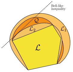
Figure 1: Pictorial representation of the sets of correlations, together with our approach to detection of multipartite nonlocality. The $\mathcal{L}$ and $\mathcal{Q}$ sets delimit the local and quantum correlations respectively. As shown here, the first forms a polytope, namely a convex set delimited by a finite amount of extremal points, while the second, despite still being convex, is not a polytope. The light orange sets are the first representatives of the hierarchy $\mathcal{L}_{1}\supseteq\mathcal{L}_{2}\supseteq{\ldots}\supseteq\mathcal{L}$ approximating the local set from outside. It can be seen that some of the quantum correlations lie outside the $\mathcal{L}_{2}$, meaning that they are detected as nonlocal from the SDP relaxation at the second level. The dotted line shows a Bell-like inequality that can be obtained by the corresponding dual problem.

V Applications

The goal of this section is to show that the SDP relaxation can be successfully employed for detection of nonlocality arising from a broad range of quantum states. We focus particularly in exploring the efficient scaling of the method in terms of number of particles. To generate the SDP relaxations, we use the software Ncpol2sdpa Wittek (2015), and we solve the SDPs with Mosek .

We collect evidence that, from a computational point of view, the main limiting factor of the technique is not time but the amount of memory required to store the moment matrix. Indeed, the longest time that is taken to run one of the codes amounts to approximately $9$ h . Despite the memory limitation, the SDP technique allows us to consider multipartite scenarios that cannot be dealt with in the standard linear program approach to check locality. Indeed, for the scenarios with $m=2,3$, we are able to detect nonlocality for systems of up to $N=29$ and $N=15$ respectively, thus overcoming the current limits of Gondzio et al. (2014).

In the following sections, we list the examples of states we consider. Given that we study cases with dichotomic measurements only, we present them in the expectation value form $\{M^{(i)}_{x_{i}}\}$.

$W$ state

As a first case, we analyze the Dicke state with a single excitation, also known as the $W$ state, namely

$$|W_{N}\rangle=\frac{1}{\sqrt{N}}(\left|0{\ldots}01\right\rangle+\left|0{\ldots}10\right\rangle{\ldots}+\left|10{\ldots}0\right\rangle).$$ (10)

Let us consider the simplest scenario of $m=2$ dichotomic measurements per party, where each observer performs the same two measurements; that is, $M_{0}^{(i)}=\sigma_{x}$ and $M_{1}^{(i)}=\sigma_{z}$ for all $i=1,{\ldots},N$. We are able to show that the obtained probability distribution is detected as nonlocal at level $\mathcal{L}_{2}$ for $N\leq 29$. We recall that in this scenario the complexity of this test scales as $O(N^{4})$, in terms of both elements to assign in the moment matrix and measurements to implement experimentally.

We also study the robustness of our technique to white noise,

$$\rho_{N}(p)=(1-p)|W_{N}\rangle\langle W_{N}|+p\frac{\mathbb{1}_{N}}{2^{N}}$$ (11)

where $0\leq p\leq 1$ and $\mathbb{1}_{N}$ represents the identity operator acting on the space of $N$ qubits. We estimate numerically the maximal value of $p$, referred to as $p_{max}$, for which the given correlations are still nonlocal according to the SDP criterion. Table 1 reports the resulting values as a function of the number of parties. While the robustness to noise decreases with the number of parties, the method tolerates realistic amounts of noise, always larger than $6\%$, for all the tested configurations.

$N$	$p_{max}$	$N$	$p_{max}$	$N$	$p_{max}$
5	0.295	14	0.141	23	0.083
6	0.296	15	0.131	24	0.079
7	0.277	16	0.122	25	0.076
8	0.251	17	0.114	26	0.073
9	0.225	18	0.107	27	0.070
10	0.202	19	0.101	28	0.068
11	0.183	20	0.096	29	0.065
12	0.167	21	0.091
13	0.153	22	0.087

Table 1: Robustness of nonlocality to white noise in the case of the $W$ state, reported as a function of $N$.

Finally, in order to study the robustness of the proposed test with respect to the choice of measurements, we also consider a situation where the parties are not able to fully align their measurements and choose randomly two orthogonal measurements Wallman et al. (2011). More precisely, we assume that $M_{0}^{(i)}=\vec{x}_{0}^{(i)}\cdot\vec{\sigma}$ and $M_{1}^{(i)}=\vec{x}_{1}^{(i)}\cdot\vec{\sigma}$, where $\vec{\sigma}=(\sigma_{x},\sigma_{y},\sigma_{z})$ and $\vec{x}_{0}^{(i)},\vec{x}_{1}^{(i)}$ are vectors chosen uniformly at random, with the only constraint of being orthogonal; namely $\vec{x}_{0}^{(i)}\cdot\vec{x}_{1}^{(i)}=0$ for all $i=1,{\ldots},N$. We calculate numerically the probability $p_{NL}$ for the corresponding correlations to be detected as nonlocal at the second level of the relaxation. To estimate $p_{NL}$, we compute the fraction $N_{NL}/N_{r}$ of $N_{NL}$ nonlocal distributions obtained over a total of $N_{r}=1000$ rounds. The corresponding results are reported in the following table as a function of $N$.

$N$	$p_{NL}$	$N$	$p_{NL}$
3	50.2 %	7	21.0 %
4	44.4 %	8	12.8 %
5	38.4 %	9	6.3 %
6	28.8 %	10	2.7 %

The results for random measurements also exemplify one of the advantages of our approach with respect to previous entanglement detection schemes. Given some observed correlations, our test can be run and sometimes detects whether the correlations are nonlocal and therefore come from an entangled state. To our understanding, reaching similar conclusions using entanglement witnesses or other entanglement criteria is much harder, as they require solving optimization problems involving $N$-qubit mixed states.

$GHZ$ state

Another well-studied multipartite state is the Greenberger-Horne-Zeilinger (GHZ) state, given by

$$|GHZ_{N}\rangle=\frac{1}{\sqrt{2}}\left(|0\rangle^{\otimes N}+|1\rangle^{\otimes N}\right).$$ (12)

Contrarily to the $W$ state, such a state is not suited for detection of nonlocality with few-body correlations because all the $k$-body distributions arising from measurements on (12) are the same as those obtained by measuring the separable mixed state $\frac{1}{2}(|0\rangle\langle 0|^{\otimes k}+|1\rangle\langle 1|^{\otimes k})$. Therefore, in order to apply our nonlocality detection method to the $GHZ$ state we need to involve at least one full-body term.

The solutions we present are inspired by the self-testing scheme for graph states introduced in McKague (2011): the first scenario involves $m=3$ dichotomic measurements per party; namely $M_{0}^{(i)}=\sigma_{x}$, $M_{1}^{(i)}=\sigma_{d}=\frac{1}{\sqrt{2}}(\sigma_{x}+\sigma_{z})$ and $M_{2}^{(i)}=\sigma_{z}$ for all $i=1,{\ldots},N$. To introduce full-body correlators in the SDP we define the set $\mathcal{O}_{mix}=\{\mathcal{O}_{2},\langle M_{0}^{(1)}M_{0}^{(2)}{\ldots}M_{0}^{(N)}\rangle,\langle M_{1}^{(1)}M_{0}^{(2)}{\ldots}M_{0}^{(N)}\rangle\}$. The moment matrix corresponding to such set represents a mixed level of the relaxation, containing also two full-body correlators in the entries. However, since the number of added columns and rows is fixed to $2$ for any $N$, this level is basically equivalent to level $\mathcal{L}_{2}$. Therefore, we preserve the efficient $O(N^{4})$ scaling with the number of parties of elements in the moment matrix and measurements to implement.

By numerically solving the SDP associated to this mixed level of the hierarchy we are able to confirm nonlocality of the correlations arising from the $GHZ$ state and the given measurement for up to $N\leq 15$ parties. Moreover, we check that the number of full-body values that is necessary to assign is constant for any of the considered $N$, coinciding with the two correlators $\langle M_{0}^{(1)}M_{0}^{(2)}{\ldots}M_{0}^{(N)}\rangle$ and $\langle M_{1}^{(1)}M_{0}^{(2)}{\ldots}M_{0}^{(N)}\rangle\$. Lastly, we estimate that the robustness to noise in this case does not depend on $N$ and it amounts to $p_{max}\approx 0.17$.

As a second scenario, we also notice that one can produce nonlocal correlations from the $GHZ$ at the level $\mathcal{O}_{mix}$ by considering $m=2$ measurement choices only. Indeed, if ones considers $M_{0}^{(i)}=\sigma_{x}$, $M_{1}^{(i)}=\sigma_{d}$, the resulting correlations are detected as nonlocal for any $N\leq 28$ (the fact that we are not able to reach $N=29$ is due to the mixed level of the relaxations, which results in a bigger matrix compared the scenario for the $W$ state). Table (2) shows the corresponding robustness to noise, computed in the same way as for the $W$ state. For both configurations, the noise robustness of our scheme in detecting GHZ states seems to saturate for large $N$ even if the computational (and experimental) effort scales polynomially.

$N$	$p_{max}$	$N$	$p_{max}$	$N$	$p_{max}$
5	0.107	14	0.135	23	0.145
6	0.112	15	0.137	24	0.146
7	0.116	16	0.138	25	0.147
8	0.120	17	0.140	26	0.147
9	0.123	18	0.141	27	0.148
10	0.127	19	0.142	28	0.148
11	0.129	20	0.143
12	0.132	21	0.144
13	0.134	22	0.145

Table 2: Robustness of nonlocality to white noise in the case of the $GHZ$ state and $2$ dicothomic measurements per party, reported as a function of $N$.

Graph states

Graph states Hein et al. (2006) constitute another important family of multipartite entangled states. Such states are defined as follows: consider a graph $G$, i.e. a set of $N$ vertices labeled by $i$ connected by some edges $\mathcal{E}_{ij}$ connecting the vertices $i$ and $j$. We associate a qubit system in the state $\left|+\right\rangle_{i}$ for each edge $i$ and apply a control-$Z$ grate $CZ_{ij}=\text{diag}(1,1,1,-1)$ to every pair of qubits $i$ and $j$ that are linked according to the graph $G$.

We notice that $GHZ$ state is also a graph state, associated to the so-called star graph. However, due to its particular relevance in quantum information, we prefer to treat its case in the previous section. Here we consider some other exemplary graph states such as the 1D and 2D cluster states and the loop graph state illustrated in Figure 2. Inspired by the self-testing scheme in McKague (2011), we consider that each party applies three measurements given by $\sigma_{x},\sigma_{z}$ and $\sigma_{d}$. We are able to detect nonlocality in the obtained correlations at level $\mathcal{L}_{2}$ for states involving up to $N=15$ qubits. Again, the method at this level scales as $N^{4}$.

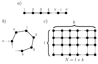
Figure 2: Representatives of the graphs associated to the classes of states that have been studied with the SDP method: a) Linear graph states. b) Loop graph states. c) 2D cluster states.

Interestingly, our approach for the detection of nonlocal correlations generated by graph states shows to be qualitatively different from McKague’s scheme in McKague (2011). While the latter requires correlators of an order that depends on the connectivity of the graph (namely, equal to $1$ plus the maximal number of neighbors that each vertex has), our method seems - at least in some cases - to be independent of it. Indeed, we are able to detect nonlocality with four-body correlators in 2D cluster states, whose connectivity would imply five-body correlators for the self-testing scheme.

VI Explicit Bell inequalities

Another nice property of our nonlocality criterion comes from the fact that, as it can be put in a SDP form, it immediately provides a method to find experimentally friendly Bell inequalities involving a subset of all possible measurements. In fact, it turns out that the the SDP proposed in Sec. III has a dual formulation that can be interpreted as the optimization of a linear function of the correlations that can be seen as a Bell-like functional, i.e. a functional that has a nontrivial bound for all correlations in $\mathcal{L}_{k}$ (Navascués et al., 2008) (see Appendix A for details). Thus, if a set of correlations is found to be nonlocal, then the solution of the SDP provides a Bell inequality that is satisfied by correlations in $\mathcal{L}_{\nu}$ and that is violated by the tested correlations. Importantly, this Bell inequality can further be used to test other sets of correlations.

By using the two sets of correlations obtained by measuring 3 dicothomic observables per party in the GHZ state we are able to find the following Bell inequality:

$$\begin{split}\mathcal{I}_{mix}^{3}=\sum_{i=2}^{N}\langle M_{1}^{(1)}M_{2}^{(i)}\rangle-\sum_{i=2}^{N}\langle M_{0}^{(1)}M_{2}^{(i)}\rangle+\\ +(N-1)\langle M_{0}^{(1)}M_{0}^{(2)}{\ldots}M_{0}^{(N)}\rangle+\\ +(N-1)\langle M_{1}^{(1)}M_{0}^{(2)}{\ldots}M_{0}^{(N)}\rangle\leq 2(N-1)\end{split}$$ (13)

Numerically, we could certify the validity of this inequality for up to $N\leq 15$. Moreover, in principle the bound of $\beta_{C}=2(N-1)$ is only guaranteed to be satisfied by correlations in $\mathcal{L}_{mix}$. However, motivated by the obtained numerical insight, we could prove that this bound actually coincides with the true local bound, and therefore, (13) is a valid Bell inequality for all $N$ (for all the analytical proofs regarding this section, see Appendix B). This shows that, at least in this instance, the $\mathcal{L}_{mix}$ defined by the SDP relaxation associated to $\mathcal{O}_{mix}$ is tight to the local set.

It is also easy to show that (13) is violated by the $GHZ$ state and the previously introduced choice of measurements. In particular, the value reached is $\mathcal{I}^{3}_{GHZ}=(1+\sqrt{2})(N-1)$ for any $N$. Given that both the local bound and the violation scale linearly with $N$, the robustness of nonlocality to white noise is constant and amounts to $p_{max}=\frac{\sqrt{2}-1}{\sqrt{2}+1}\approx 0.174$. We note that this results is in agreement with what is achieved numerically with the SDP for up to $N=15$.

Similarly, we also find the following Bell inequality by using the set of correlations involving only two measurements per party described for the GHZ state:

$$\begin{split}\mathcal{I}_{mix}^{2}=\sum_{i=2}^{N}\langle M_{1}^{(1)}M_{1}^{(i)}\rangle-\sum_{i=2}^{N}\langle M_{0}^{(1)}M_{1}^{(i)}\rangle+\\ +(N-1)\langle M_{0}^{(1)}M_{0}^{(2)}{\ldots}M_{0}^{(N)}\rangle+\\ +(N-1)\langle M_{1}^{(1)}M_{0}^{(2)}{\ldots}M_{0}^{(N)}\rangle\leq 2(N-1)\end{split}$$ (14)

Once more, although this inequality is found numerically for up to $N\leq 28$ we prove that it is valid for any $N$. Moreover the bound $\beta_{C}=2(N-1)$ is not only valid for correlation in $\mathcal{L}_{mix}$ but for any local set of correlations. The $GHZ$ state and the given measurements result in a violation of $\mathcal{I}_{GHZ}^{2}=\frac{3+\sqrt{2}}{2}$. Given that in this case the relative violation is lower, we also have a lower robustness to noise, coinciding with $p_{max}=\frac{\sqrt{2}-1}{\sqrt{2}+3}\approx 0.09$ for any $N$. We notice that this value is different from the ones reported in Table (2). The reason is that, to derive inequality (14) from the dual, we restrict to assign only the values of the two-body correlations and the two full-body ones. On the other hand, the results in Table (2) also take into account the assignment of the three- and four-body correlators, showing that this additional knowledge helps in improving the robustness to noise.

As a final remark, we stress that the measurement settings considered to derive an inequality from the dual might not be the optimal ones. For instance, we are able to identify different measurement choices for the case of (14) that lead to a higher violation of such an inequality, hence resulting also in a better robustness to noise (see Appendix B for details).

VII Discussion

We introduce a technique for efficient device-independent entanglement detection for multipartite quantum systems. It relies on a hierarchy of necessary conditions for nonlocality in the observed correlations. By focusing on the second level of the hierarchy, we consider a test that requires knowledge of up to four-body correlators only. We show that it can be successfully applied to detect entanglement of many physically relevant states, such as the $W$, the $GHZ$ and the graph states. Besides being suitable for experimental implementation, our technique also has an efficient scaling in terms of computational requirements, given that the number of variables involved grows polynomially with $N$. This allows us to overcome the limitation of the currently known methods and to detect entanglement for states of up to few tens of particles. Moreover, the proposed technique has a completely general approach and it can be applied to any set of observed correlations. This makes it particularly relevant for the detection of new classes of multipartite entangled states.

We note that our techniques can also be used as a semidefinite constraints to impose locality. Consider, for instance, a linear function $f$ of the observed correlations. One could find an upper bound on the value of this function over local correlations by maximizing it under the constraint that the moment matrix $\Gamma$ is positive semidefinite. A particular example could be to take $f$ to be a Bell polynomial. Thus this approach would find a bound $f\leq\beta_{C}$ satisfied by all local correlations.

As a future question in this direction, it would be interesting to study how accurate is the approximation of the local set of correlations provided by the second level of the hierarchy. In some of the scenario that we consider the approximation is actually tight, but this is not generally the case. A possible approach could be to compare the local bound of some known Bell inequalities with that resulting from the hierarchy.

Furthermore, we notice that the second level of the hierarchy also has an efficient scaling with the number of measurements performed by the parties. This would allow us to inquire whether an increasing number of measurement choices can provide an advantage for entanglement detection in multipartite systems.

Lastly, we believe that the present techniques can be readily applied in current state-of-the-art experiments. For instance, experiments composed by up to 7 ions have demonstrated nonlocality using an exponentially increasing number of full correlators Lanyon et al. (2014). Moreover, recent experiments have produced GHZ-like states in systems composed by 14 ions Monz et al. (2011) and 10 photons Wang et al. (2016); Chen et al. (2017) with visibilities within the range required to observe a violation of the Bell inequalities presented here. We notice, however, that the measurements required to certify the presence of nonlocal correlations using our approach are different from the ones reported in these works.

VIII Acknowledgements

The authors thank J. Kaniewski and the referees for helpful comments. D.C. thanks R. Chaves for discussions and hospitality at the International Institute of Physics (Natal-Brazil). This work was supported by the ERC CoG grant QITBOX, Spanish MINECO (Severo Ochoa grant SEV-2015-0522, a Ramón y Cajal fellowship, a Severo Ochoa PhD fellowship, QIBEQI FIS2016-80773-P and FOQUS FIS2013-46768-P), the AXA Chair in Quantum Information Science, the Generalitat de Catalunya (SGR875 and CERCA Program) and Fundacion Cellex. The authors also acknowledge the computational resources granted by the High Performance Computing Center North (SNIC 2016/1-320).

Appendix A Details of the method

Here, we present in more detail the SDP relaxation associated to quantum realizations with commuting measurements. In order to be consistent with the examples presented in the main text, we express it in terms of correlators, but we stress that a formulation in terms of projector and probabilities for higher numbers of outcomes is straightforward.

Let us consider that the $N$ observers $A_{i}$ are allowed to perform $m$ dicothomic measurements each. We can therefore define the operators $M^{(i)}_{x_{i}}=M^{1}_{x_{i}}-M^{0}_{x_{i}}$ in terms of measurements $M^{a_{i}}_{x_{i}}$. It can be easily seen that expectation values of $M^{(i)}_{x_{i}}$ correspond to the correlators (3).

For any quantum realization of such operators, it is possible to show that they satisfy the following properties:

1. $(M^{(i)}_{x_{i}})^{\dagger}$ = $M^{(i)}_{x_{i}}$ for any $i=1,{\ldots}N$ and $x_{i}=1,{\ldots},m$,

2. $(M^{(i)}_{x_{i}})^{2}=\mathbb{1}$ for any $i=1,{\ldots}N$ and $x_{i}=1,{\ldots},m$,

3. $[M^{(i)}_{x_{i}},M^{(j)}_{x_{j}}]=0\,\,\,$ for any $i\neq j$ and $x_{i},x_{j}=1,{\ldots},m$.

Now, let us consider that the sets $\mathcal{O}_{\nu}$ we introduce in section III consist exactly of all the products of the $\{M^{(i)}_{x_{i}}\}$ up to order $\nu$. Then, by indexing the operators in the sets as $\mathcal{O}_{i}$ for $i=1,{\ldots},k$, we define the $k\times k$ moment matrix as follows

$$\Gamma_{ij}=tr(\rho_{N}\mathcal{O}^{\dagger}_{i}\mathcal{O}_{j})$$

where $\rho_{N}$ is a generic N-partite quantum state. As it was shown in (Navascués et al., 2007, 2008), for any set of quantum correlations $P$, the properties i)-iii) and the fact that the associated $\rho_{N}$ is a proper quantum state reflect into the following properties of the moment matrix:

• $\Gamma^{\dagger}=\Gamma$,

• $\Gamma\succeq 0$,

• the entries of the matrix are constrained by some linear equations of the form

  $$\sum_{i,j}(F_{m})_{ij}\Gamma_{ij}=g_{m}(P)\,\,\,\,m=1,{\ldots},l$$

  where $(F_{m})_{ij}$ are some coefficients and the $g_{m}(P)$ can depend on the values of the correlators composing the $P$ vector, as such

  $$g_{m}(P)=(g_{m})_{0}+\sum_{k=1}^{N}\sum_{\begin{subarray}{c}i_{1}<{\ldots}<i_{k}\\ i_{1},{\ldots},i_{j}\end{subarray}}(g_{m})^{i_{1},{\ldots},i_{k}}_{j_{1},{\ldots}j_{k}}\langle M_{j_{1}}^{(i_{1})}{\ldots}M_{j_{k}}^{(i_{k})}\rangle$$

Up to this point, the method we describe coincides with the NPA hierarchy (Navascués et al., 2007, 2008), which is used to check whether a set of observed correlations is compatible with a quantum realization. In order to define a hierarchy to test for local hidden variables realization, we introduce the additional condition that all the measurements for the same party have to also be commuting, namely

1. $[M_{x_{i}}^{(i)},M_{y_{i}}^{(i)}]=0\,\,\$ for any $i=1,{\ldots},N$ and $x_{i}\neq y_{i}=1,{\ldots},m$.

It can be seen that property iv) implies a second set of linear constraints on the $\Gamma$ matrix, which we identify as

$$\sum_{i,j}(F{{}^{\prime}}_{m})_{ij}\Gamma_{ij}=g{{}^{\prime}}_{m}(P)\,\,\,\,m=1,{\ldots},l{{}^{\prime}}$$

To make it clearer, we show an example of linear constraint that can come only if we impose condition iv). Let us consider the following four operators: $\mathcal{O}_{k}=M_{x_{i}}^{(i)}M_{y_{i}}^{(i)}$, $\mathcal{O}_{l}=M_{x_{i}}^{(i)}M_{x_{j}}^{(j)}$, $\mathcal{O}_{n}=M_{y_{i}}^{(i)}$ and $\mathcal{O}_{m}=M_{x_{j}}^{(j)}$. It is easy to see that, by exploiting i)-iii) plus iv), $\Gamma_{kl}=\Gamma_{nm}$ for any choice of $x_{i},y_{i},x_{j}=1,{\ldots},m$ and $i,j=1,{\ldots},N$.

Now, for any chosen $\mathcal{O}_{\nu}$, we can test whether an observed distribution $P$ is compatible with a local model via the following SDP

maximize $$\,\,\,\lambda,$$

subject to $$\,\,\,\Gamma-\lambda\mathbb{1}\succeq 0,$$

$$\,\,\sum_{i,j}(F_{m})_{ij}\Gamma_{ij}=g_{m}(P)\,\,\,\,m=1,{\ldots},l\,\,,$$ (15)

$$\,\,\sum_{i,j}(F{{}^{\prime}}_{m})_{ij}\Gamma_{ij}=g{{}^{\prime}}_{m}(P)\,\,\,\,m=1,{\ldots},l{{}^{\prime}}\,\,,$$

which is the primal form of the problem. A solution $\lambda^{\ast}_{min}<0$ implies that it is not possible to find a semidefinite positive moment matrix satisfying the given linear constraints. Therefore $P$ has no quantum realization with commuting measurements and we conclude it is nonlocal. We notice that by increasing the value of $\nu$ we get a sequence of more and more stringent tests for nonlocality. Indeed, the linear constraints for the level $\nu$ are always a subset of the ones coming from $\nu+1$. Moreover, in analogy with the NPA hierarchy, the series of tests is convergent; hence any nonlocal correlation will give a negative solution $\lambda^{\ast}_{min}$ at a finite step of the sequence.

Interestingly, we can also study the dual form of the SDP problem, which reads as follows:

minimize $$\,\,\,G(P)=\sum_{k}y_{k}g_{k}(P)+\sum_{k}y{{}^{\prime}}_{k}g{{}^{\prime}}_{k}(P),$$

subject to $$\,\,\,\sum_{k}y_{k}F^{T}_{k}+\sum_{k}y{{}^{\prime}}_{k}F{{}^{\prime}}^{T}_{k}\succeq 0,$$ (16)

$$\,\,\,\sum_{k}y_{k}\text{tr}(F^{T}_{k})+\sum_{k}y{{}^{\prime}}_{k}\text{tr}(F{{}^{\prime}}^{T}_{k})=1.$$

Thanks to the strong duality of the problem, a negative solution for the primal implies also $G(P)=\lambda^{\ast}_{min}<0$. Since any point in $\mathcal{L}_{\nu}$ satisfies the SDP condition at level $\nu$ with $G(P)\geq 0$, we can interpret $G(P)$ as a Bell-like inequality separating the $\mathcal{L}_{\nu}$ from the rest of the correlations. Indeed, since $g_{k}(P)$ and $g{{}^{\prime}}_{k}(P)$ are linear in terms of the probability distribution, we derive that $G(P)\geq 0$ defines also a linear inequality for $P$. Violation of such an inequality directly implies nonlocality.

Appendix B Proof of local bound and quantum violation for the inequalities

We start by proving the local bounds for the inequalities introduced in the main text. To do so, we remind the reader that to derive the maximal value attained by local correlations it is enough to maximize over the vertices of the local set. In the correlator space, the deterministic local strategies (DLS) take the form

$$\langle M_{j_{1}}^{(i_{1})}{\ldots}M_{j_{k}}^{(i_{k})}\rangle=\langle M_{j_{1}}^{(i_{1})}\rangle{\ldots}\langle M_{j_{k}}^{(i_{k})}\rangle$$ (17)

where each $M_{x_{i}}^{(i)}$ term can take only $1$ and $-1$ values. By using this property, inequality (13) becomes

$$\begin{split}\mathcal{I}_{mix}^{3}(DLS)=(N-1)\left[\langle M_{1}^{(1)}\rangle+\langle M_{0}^{(1)}\rangle\right]\mathcal{T}_{0}\\ +\left[\langle M_{1}^{(1)}\rangle-\langle M_{0}^{(1)}\rangle\right]\mathcal{T}_{2}\end{split}$$ (18)

where $\mathcal{T}_{0}=\langle M_{0}^{(2)}\rangle{\ldots}\langle M_{0}^{(N)}\rangle$ and $\mathcal{T}_{2}=\sum_{i=2}^{N}\langle M_{2}^{(i)}\rangle$. For any number of parties $N$, we have that $\mathcal{T}_{0}\leq 1$ and $\mathcal{T}_{2}\leq N-1$; therefore

$$\mathcal{I}_{mix}^{3}(DLS)\leq 2(N-1)\langle M_{1}^{(1)}\rangle\leq 2(N-1)$$ (19)

Similarly, for any deterministic strategy, inequality (14) takes the from

$$\begin{split}\mathcal{I}_{mix}^{2}(DLS)=(N-1)\left[\langle M_{1}^{(1)}\rangle+\langle M_{0}^{(1)}\rangle\right]\mathcal{T}_{0}\\ +\left[\langle M_{1}^{(1)}\rangle-\langle M_{0}^{(1)}\rangle\right]\mathcal{T}_{1}\end{split}$$ (20)

where $\mathcal{T}_{1}=\sum_{i=2}^{N}\langle M_{1}^{(i)}\rangle$. As for before, we can use the argument that $\mathcal{T}_{0}\leq 1$ and $\mathcal{T}_{1}\leq N-1$ to conclude

$$\mathcal{I}_{mix}^{2}(DLS)\leq 2(N-1)\langle M_{1}^{(1)}\rangle\leq 2(N-1)$$ (21)

Regarding the quantum violation, we recall that the scenario we consider is $|\psi\rangle=|GHZ_{N}\rangle=\frac{1}{\sqrt{2}}(|0\rangle^{\otimes N}+|1\rangle^{\otimes N})$ with measurements choices $M_{0}^{(i)}=\sigma_{x}$, $M_{1}^{(i)}=\sigma_{d}=\frac{1}{\sqrt{2}}(\sigma_{x}+\sigma_{z})$ and $M_{2}^{(i)}=\sigma_{z}$ for all $i=1,{\ldots},N$. It is easy to check that, for a $GHZ$ state of any number of parties, the following is true

• $\langle\sigma_{x}^{(i)}\sigma_{x}^{(j)}\rangle=\langle\sigma_{x}^{(i)}\sigma_{z}^{(j)}\rangle=0$ for any $i\neq j=1,{\ldots},N$.

• $\langle\sigma_{z}^{(i)}\sigma_{z}^{(j)}\rangle=1$ and therefore $\langle\sigma_{d}^{(i)}\sigma_{z}^{(j)}\rangle=\frac{1}{\sqrt{2}}$ and $\langle\sigma_{d}^{(i)}\sigma_{d}^{(j)}\rangle=\frac{1}{2}$for any $i\neq j=1,{\ldots},N$.

• $\langle\sigma_{x}^{(1)}\sigma_{x}^{(2)}{\ldots}\sigma_{x}^{(N)}\rangle=1$ and $\langle\sigma_{z}^{(1)}\sigma_{x}^{(2)}{\ldots}\sigma_{x}^{(N)}\rangle=0$, therefore $\langle\sigma_{d}^{(1)}\sigma_{x}^{(2)}{\ldots}\sigma_{x}^{(N)}\rangle=\frac{1}{\sqrt{2}}$ for any $N$.

By using the properties listed above, one can check that

$$\langle\mathcal{I}_{mix}^{3}\rangle_{GHZ_{N}}=(1+\sqrt{2})(N-1)\approx 2.41(N-1)$$ (22)

and, similarly, that

$$\langle\mathcal{I}_{mix}^{2}\rangle_{GHZ_{N}}=\frac{3+\sqrt{2}}{2}(N-1)\approx 2.21(N-1)$$ (23)

Moreover, we notice that by changing the measurement setting, one can achieve a higher violation of $\mathcal{I}_{mix}^{2}$. Indeed, it is easy to see that by choosing $M_{0}^{(1)}=\frac{1}{\sqrt{2}}(\sigma_{x}+\sigma_{z})$, $M_{1}^{(1)}=\frac{1}{\sqrt{2}}(\sigma_{x}-\sigma_{z})$ and $M_{0}^{(i)}=\sigma_{x}$,$M_{1}^{(i)}=\sigma_{z}$ for $i=2,{\ldots},N$, the resulting violation is

$$\langle\mathcal{I}_{mix}^{2}\rangle_{GHZ_{N}}=2\sqrt{2}(N-1)\approx 2.83(N-1)$$ (24)

To conclude, we proceed with the analysis of the robustness to noise. We recall that this implies considering the noisy version of the $GHZ$ state; namely

$$\rho_{N}(p)=(1-p)\rho_{GHZ_{N}}+p\frac{\mathbb{1}_{N}}{2^{N}}$$ (25)

where $0\leq p\leq 1$ represent the amount of white noise added to the state. It can be easily seen that the noise affects the values of the correlators for the $GHZ$ state in the following way

$$\langle\sigma_{j_{1}}^{(i_{1})}{\ldots}\sigma_{j_{k}}^{(i_{k})}\rangle_{\rho_{N}}=(1-p)\langle\sigma_{j_{1}}^{(i_{1})}{\ldots}\sigma_{j_{k}}^{(i_{k})}\rangle_{GHZ_{N}}$$ (26)

for any $j_{l}\in\{x,y,z\}$ and $1\leq k\leq N$. Therefore we can consider the noise as a simple damping factor in the violation of the inequalities. By using this fact, we get that $\mathcal{I}_{mix}^{3}$ is violated as long as $(1-p)(1+\sqrt{2})(N-1)>2(N-1)$; hence

$$p_{max}(\mathcal{I}_{mix}^{3})=\frac{\sqrt{2}-1}{\sqrt{2}+1}\approx 0.17$$ (27)

By the same argument, we analyze $\mathcal{I}_{mix}^{2}$ for the two measurements settings that we introduce. For the first one, the inequality is violated as long as $(1-p)\frac{3+\sqrt{2}}{2}(N-1)>2(N-1)$ and, therefore,

$$p_{max}(\mathcal{I}_{mix}^{2})=\frac{\sqrt{2}-1}{\sqrt{2}+3}\approx 0.09$$ (28)

while for the second one, the violation is preserved for $(1-p)2\sqrt{2}(N-1)>2(N-1)$; hence

$$p^{\prime}_{max}(\mathcal{I}_{mix}^{2})=1-\frac{\sqrt{2}}{2}\approx 0.29$$ (29)

Clearly, we see that for the second setting a higher violation results also in a significantly higher robustness to noise.

References

- Bennett et al. (1993) Charles H. Bennett, Gilles Brassard, Claude Crépeau, Richard Jozsa, Asher Peres, and William K. Wootters, “Teleporting an unknown quantum state via dual classical and einstein-podolsky-rosen channels,” Physical Review Letters 70, 1895–1899 (1993).
- Ekert (1991) Artur K. Ekert, “Quantum cryptography based on Bell’s theorem,” Physical Review Letters 67, 661–663 (1991).
- Briegel et al. (2009) H J Briegel, D E Browne, W Dür, R Raussendorf, and M Van den Nest, “Measurement-based quantum computation,” Nature Physics 5, 19–26 (2009).
- Giovannetti et al. (2004) Vittorio Giovannetti, Seth Lloyd, and Lorenzo Maccone, “Quantum-enhanced measurements: beating the standard quantum limit.” Science 306, 1330–6 (2004).
- Horodecki et al. (2009) Ryszard Horodecki, Paweł Horodecki, Michał Horodecki, and Karol Horodecki, “Quantum entanglement,” Review of Modern Physics 81, 865–942 (2009).
- Häffner et al. (2005) H Häffner, W Hänsel, CF Roos, J Benhelm, M Chwalla, T Körber, UD Rapol, M Riebe, PO Schmidt, C Becher, et al., “Scalable multiparticle entanglement of trapped ions,” Nature 438, 643–646 (2005).
- Brandão and Christandl (2012) Fernando G S L Brandão and Matthias Christandl, “Detection of multiparticle entanglement: Quantifying the search for symmetric extensions,” Physical Review Letters 109, 160502 (2012).
- Bourennane et al. (2004) Mohamed Bourennane, Manfred Eibl, Christian Kurtsiefer, Sascha Gaertner, Harald Weinfurter, Otfried Gühne, Philipp Hyllus, Dagmar Bruß, Maciej Lewenstein, and Anna Sanpera, “Experimental detection of multipartite entanglement using witness operators,” Physical Review Letters 92, 087902 (2004).
- Tóth and Gühne (2006) G. Tóth and O. Gühne, “Detection of multipartite entanglement with two-body correlations,” Applied Physics B: Lasers and Optics 82, 237–241 (2006).
- Lücke et al. (2014) Bernd Lücke, Jan Peise, Giuseppe Vitagliano, Jan Arlt, Luis Santos, Géza Tóth, and Carsten Klempt, “Detecting multiparticle entanglement of Dicke states,” Physical Review Letters 112, 155304 (2014).
- Vitagliano et al. (2014) Giuseppe Vitagliano, Iagoba Apellaniz, Iñigo L. Egusquiza, and Géza Tóth, “Spin squeezing and entanglement for an arbitrary spin,” Physical Review A 89, 032307 (2014).
- Jungnitsch et al. (2011) Bastian Jungnitsch, Tobias Moroder, and Otfried Gühne, “Taming multiparticle entanglement,” Physical Review Letters 106, 190502 (2011).
- Knips et al. (2016) Lukas Knips, Christian Schwemmer, Nico Klein, Marcin Wieśniak, and Harald Weinfurter, “Multipartite entanglement detection with minimal effort,” Physical Review Letters 117, 210504 (2016).
- Apellaniz et al. (2017) Iagoba Apellaniz, Matthias Kleinmann, Otfried Gühne, and Géza Tóth, “Optimal witnessing of the quantum fisher information with few measurements,” Physical Review A 95, 032330 (2017).
- Bell (1964) John Stewart Bell, “On the Einstein-Podolsky-Rosen paradox,” Physics 1, 195–200 (1964).
- Brunner et al. (2014) Nicolas Brunner, Daniel Cavalcanti, Stefano Pironio, Valerio Scarani, and Stephanie Wehner, “Bell nonlocality,” Reviews of Modern Physics 86, 419 (2014).
- Zukowski et al. (1999) Marek Zukowski, Dagomir Kaszlikowski, Adam Baturo, and Jan-Ake Larsson, “Strengthening the Bell theorem: conditions to falsify local realism in an experiment,” arXiv quant-ph/9910058 (1999).
- Fine (1982) Arthur Fine, “Hidden variables, joint probability, and the Bell inequalities,” Physical Review Letters 48, 291–295 (1982).
- Navascués et al. (2007) Miguel Navascués, Stefano Pironio, and Antonio Acín, “Bounding the set of quantum correlations,” Physical Review Letters 98, 010401 (2007).
- Navascués et al. (2008) Miguel Navascués, Stefano Pironio, and Antonio Acín, “A convergent hierarchy of semidefinite programs characterizing the set of quantum correlations,” New Journal of Physics 10, 073013 (2008).
- Kogias et al. (2015) Ioannis Kogias, Paul Skrzypczyk, Daniel Cavalcanti, Antonio Acín, and Gerardo Adesso, “Hierarchy of steering criteria based on moments for all bipartite quantum systems,” Physical Review Letters 115, 210401 (2015).
- Cavalcanti and Skrzypczyk (2017) D Cavalcanti and P Skrzypczyk, “Quantum steering: a review with focus on semidefinite programming,” Reports on Progress in Physics 80, 024001 (2017).
- Pironio et al. (2010) Stefano Pironio, Miguel Navascués, and Antonio Acín, “Convergent relaxations of polynomial optimization problems with noncommuting variables,” SIAM J. Optim. 20, 2157–2180 (2010).
- Doherty et al. (2008) Andrew C. Doherty, Yeong-Cherng Liang, Ben Toner, and Stephanie Wehner, “The quantum moment problem and bounds on entangled multi-prover games,” Proc. IEEE 23rd Annual Conf. Comp. Compl. , 199–210 (2008).
- Lasserre (2001) Jean B Lasserre, “Global optimization with polynomials and the problem of moments,” SIAM Journal on Optimization 11, 796–817 (2001).
- Steeg and Galstyan (2011) Greg Ver Steeg and Aram Galstyan, “A sequence of relaxations constraining hidden variable models,” arXiv:1106.1636 (2011).
- Cleve et al. (2004) Richard Cleve, Peter Høyer, Benjamin Toner, and John Watrous, “Consequences and limits of nonlocal strategies,” in Computational Complexity, 2004. Proceedings. 19th IEEE Annual Conference on (IEEE, 2004) pp. 236–249.
- Note (1) A more formal way to see it is to notice that we are restricting the projective algebra of NPA by the commutation condition. Then, given that the original algebra already meets the Archimedean condition, the convergence holds for the commuting case as well.
- Collins and Gisin (2004) Daniel Collins and Nicolas Gisin, “A relevant two qubit Bell inequality inequivalent to the CHSH inequality,” Journal of Physics A: Mathematical and General 37, 1775 (2004).
- Clauser et al. (1969) John F. Clauser, Michael A. Horne, Abner Shimony, and Richard A. Holt, “Proposed experiment to test local hidden-variable theories,” Physical Review Letters 23, 880–884 (1969).
- Boyd and Vandenberghe (2004) Stephen Boyd and Lieven Vandenberghe, Convex optimization (Cambridge university press, 2004).
- Gondzio et al. (2014) Jacek Gondzio, Jacek A Gruca, JA Julian Hall, Wiesław Laskowski, and Marek Żukowski, “Solving large-scale optimization problems related to Bell’s theorem,” Journal of Computational and Applied Mathematics 263, 392–404 (2014).
- Wittek (2015) Peter Wittek, “Algorithm 950: Ncpol2sdpa—sparse semidefinite programming relaxations for polynomial optimization problems of noncommuting variables,” ACM Trans. Math. Softw. 41, 21:1–21:12 (2015).
- Note (2) Available at http://www.mosek.com/.
- Note (3) The code used is available under an open source license at https://github.com/FlavioBaccari/Hierarchy-for-nonlocality-detection.
- Wallman et al. (2011) Joel J Wallman, Yeong-Cherng Liang, and Stephen D Bartlett, “Generating nonclassical correlations without fully aligning measurements,” Physical Review A 83, 022110 (2011).
- McKague (2011) Matthew McKague, “Self-testing graph states,” in Conference on Quantum Computation, Communication, and Cryptography (Springer, 2011) pp. 104–120.
- Hein et al. (2006) M. Hein, W. Dür, J. Eisert, R. Raussendorf, M. Van den Nest, and H. . Briegel, “Entanglement in Graph States and its Applications,” arXiv:quant-ph/0602096 (2006).
- Lanyon et al. (2014) B. P. Lanyon, M. Zwerger, P. Jurcevic, C. Hempel, W. Dür, H. J. Briegel, R. Blatt, and C. F. Roos, “Experimental violation of multipartite Bell inequalities with trapped ions,” Physical Review Letters 112, 100403 (2014).
- Monz et al. (2011) Thomas Monz, Philipp Schindler, Julio T. Barreiro, Michael Chwalla, Daniel Nigg, William A. Coish, Maximilian Harlander, Wolfgang Hänsel, Markus Hennrich, and Rainer Blatt, “14-qubit entanglement: Creation and coherence,” Physical Review Letters 106, 130506 (2011).
- Wang et al. (2016) Xi-Lin Wang, Luo-Kan Chen, W. Li, H.-L. Huang, C. Liu, C. Chen, Y.-H. Luo, Z.-E. Su, D. Wu, Z.-D. Li, H. Lu, Y. Hu, X. Jiang, C.-Z. Peng, L. Li, N.-L. Liu, Yu-Ao Chen, Chao-Yang Lu, and Jian-Wei Pan, “Experimental ten-photon entanglement,” Physical Review Letters 117, 210502 (2016).
- Chen et al. (2017) Luo-Kan Chen, Zheng-Da Li, Xing-Can Yao, Miao Huang, Wei Li, He Lu, Xiao Yuan, Yan-Bao Zhang, Xiao Jiang, Cheng-Zhi Peng, Li Li, Nai-Le Liu, Xiongfeng Ma, Chao-Yang Lu, Yu-Ao Chen, and Jian-Wei Pan, “Observation of ten-photon entanglement using thin BiB3O6 crystals,” Optica 4, 77–83 (2017).