Performance and Compensation of I/Q Imbalance in Differential STBC-OFDM

Abstract

Differential space time block coding (STBC) achieves full spatial diversity and avoids channel estimation overhead. Over highly frequency-selective channels, STBC is integrated with orthogonal frequency division multiplexing (OFDM) to achieve high performance. However, low-cost implementation of differential STBC-OFDM using direct-conversion transceivers is sensitive to In-phase/Quadrature-phase imbalance (IQI). In this paper, we quantify the performance impact of IQI at the receiver front-end on differential STBC-OFDM systems and propose a compensation algorithm to mitigate its effect. The proposed receiver IQI compensation works in an adaptive decision-directed manner without using known pilots or training sequences, which reduces the rate loss due to training overhead. Our numerical results show that our proposed compensation algorithm can effectively mitigate receive IQI in differential STBC-OFDM.

I Introduction

Space-time block-coded orthogonal frequency-division multiplexing (STBC-OFDM) is an effective transceiver structure to mitigate the wireless channel’s frequency selectivity while realizing multipath and spatial diversity gains [1].

To acquire channel knowledge for signal detection at the receiver, STBC-OFDM schemes require the transmission of pilot symbols [2]. However, to avoid the rate loss due to pilot signal overhead, we may want to forego channel estimation in order to reduce the increased cost of channel estimation and the degradation of tracking quality in a fast time-varying environment [3, 4]. Differential STBC transmission/detection achieves this goal and has been successfully integrated with STBC-OFDM [3, 2, 5].

Although a differential STBC-OFDM system avoids the overhead of channel estimation, a low-cost transceiver implementation based on the direct-conversion architecture suffers from analog/RF impairments. The impairments in the analog components are mainly due to the uncontrollable fabrication process variations. Since most of these impairments cannot be effectively eliminated in the analog domain, an efficient compensation algorithm in the digital baseband domain would be highly desirable for designing such low-cost wireless transceivers. One of the main sources of the analog components impairments is the imbalance between the In-phase (I) and Quadrature-phase (Q) branches when the received radio-frequency (RF) signal is down-converted to baseband. The I/Q imbalance (IQI) arises due to mismatches between the I and Q branches from the ideal case, i.e., from the exact $90^{o}$ phase difference and equal amplitudes between the sine and cosine branches. In OFDM systems, IQI destroys the subcarriers orthogonality by introducing inter-carrier interference (ICI) between mirror subcarriers which can lead to serious performance degradation [6].

Several papers investigated IQI in single-input single-output OFDM system (see [6][7] and the references therein). There are also several works dealing with IQI in coherent multiple-antenna systems. In [8], a super-block structure for the Alamouti STBC scheme is designed to ensure orthogonality in the presence of IQI. In [9], an Expectation-Maximization-based algorithm is proposed to deal with IQI in Alamouti-based STBC-OFDM systems. An equalization algorithm is proposed to overcome IQI in STBC-OFDM systems in [10]. The authors in [11] analyze and compensate IQI in single-carrier STBC systems.

Although the compensation of IQI in STBC-OFDM systems is well studied, all existing works deal with IQI either a) in coherent system, where the channel state information (CSI) is known or estimated at the receiver; or b) in a blind sense, where the signal is recovered by some statistical method based on signal properties (such as constant-modulus or circularity) [12]. To the best of our knowledge, there is no previous work dealing with IQI in differential transmission systems. Although blind estimation also does not require channel state information for detection, the input symbols are not differentially encoded and decoded and blind compensation algorithms suffer from local optima and very slow convergence. In this paper, we analyze the impact of the receiver IQI (RX-IQI) in differential STBC-OFDM (DSTBC-OFDM) systems and propose an adaptive decision-directed scheme that compensates for RX-IQI without knowing or estimating the channel information. The rest of this paper is organized as follows

The system model of DSTBC-OFDM is developed in Section II. In Section III, we formulate the problem of RX-IQI in DSTBC-OFDM and discuss the impact of RX-IQI on the bit error rate (BER) performance of DSTBC-OFDM. We propose a decision-directed IQI compensation algorithm in Section IV and the numerical results are presented in Section V. Finally, we conclude our paper in Section VI.

Notations: Unless further noted, matrices and vectors are denoted by upper-case and lower-case boldface, respectively. We denote the Hermitian, i.e. complex-conjugate transpose of a matrix or a vector by ${{(\cdot)}^{H}}$. The conjugate and transpose of a matrix, a vector, or a scalar is denoted by ${{(\cdot)}^{*}}$ and ${{(\cdot)}^{T}}$, respectively. The symbol ${{[\mathbf{A}]}_{m,n}}$ denotes the entry at the $m$-th row and the $n$-th column of matrix $\mathbf{A}$. Matrix $\mathbf{F}$ is the $N$-point Discrete Fourier Transform (DFT) matrix whose entries are given by: ${{[\mathbf{F}]}_{m,n}}=\frac{1}{\sqrt{N}}\exp(-j\frac{2\pi}{N}mn)$, with $0\leq m,n\leq N-1$. $\textrm{Re}\{\cdot\}$ and $\textrm{Im}\{\cdot\}$ denote the real and image parts of a complex number, respectively.

II System Model

We consider an Alamouti-based STBC-OFDM wireless communication system equipped with two transmit antennas and a single receive antenna. In STBC-OFDM systems, the modulated sequence is divided into $K$ blocks of a length of $2N$ symbols (where $N$ is a power of $2$) encoded by a space-time block encoder to be transmitted over the $\left(2k+1\right)$-th and $\left(2k+2\right)$-th OFDM symbols ($k=0,\cdots,K-1$). We choose the $2\times 2$ Alamouti STBC structure [13] as the core STBC due to its orthogonality advantages. In Alamouti STBC-OFDM, two complex information symbols ($x_{1}$ and $x_{2}$) drawn from a constant modulus signal constellation $\varPsi$ are simultaneously transmitted from two transmit antennas for the data block index $k$ over the $\left(2k+1\right)$-th and $\left(2k+2\right)$-th OFDM symbols.

For each two consecutive OFDM symbols, we define the $2\times 1$ vectors $\mathbf{u}_{k}^{\left(1\right)}\left(n\right)$ and $\mathbf{u}_{k}^{\left(2\right)}\left(n\right)$ to be the information vectors at the $n$-th subcarrier ($n=1,\cdots,N$) over the $\left(2k+1\right)$-th and $\left(2k+2\right)$-th OFDM symbols, respectively. Hence, the $2\times 2$ Alamouti STBC information matrix $\mathbf{U}_{k}(n)$ at the $n$-th subcarrier over the $\left(2k+1\right)$-th and $\left(2k+2\right)$-th OFDM symbols is given by $\mathbf{U}_{k}(n)\triangleq\left[\mathbf{u}_{k}^{\left(1\right)}\left(n\right)\>\brokenvert\>\mathbf{u}_{k}^{\left(2\right)}\left(n\right)\right]$ whose columns, $\mathbf{u}_{k}^{\left(1\right)}\left(n\right)$ and $\mathbf{u}_{k}^{\left(2\right)}\left(n\right)$, are defined as follows

$$\mathbf{u}_{k}^{\left(1\right)}\left(n\right) =\left[\begin{array}[]{cc}x_{1}&-x_{2}^{*}\end{array}\right]^{T}\mathbf{u}_{k}^{\left(2\right)}\left(n\right)=\left[\begin{array}[]{cc}x_{2}&x_{1}^{*}\end{array}\right]^{T}$$ (3)

where the columns of $\mathbf{U}_{k}(n)$ correspond to the information data to be transmitted from the two transmit antennas over the $\left(2k+1\right)$-th and $\left(2k+2\right)$-th OFDM symbols, respectively. Then, the output of the STBC encoder block is further passed through a serial-to-parallel converter producing two streams of data blocks of length $N$, with $N$ being the number of subcarriers. Each block is applied to a per-stream $N$-point Inverse Discrete Fourier Transform (IDFT). To avoid intersymbol interference (ISI), a cyclic prefix (CP) of length $\nu$ is added to the $N$ time-domain IDFT-output samples, resulting in an OFDM symbol of length $N+\nu$. We model the frequency-selective fading channel between the $i$-th transmit antenna and the single receive antenna as a finite impulse response (FIR) filter with $L+1$ independent taps $i.e.$ $\mbox{ }\mathbf{h}_{i}=[h_{0}^{\left(i\right)}\,h_{1}^{\left(i\right)}\,\cdots\,h_{L}^{\left(i\right)}]{}^{T}$ where $L\leq\nu$ to preserve the orthogonality between the subcarriers.

Without loss of generality, we consider the block index $k=0$ transmitted over the $1^{st}$ and $2^{nd}$ OFDM symbols, respectively, hence, we omit the index $k$ for simplicity. However, the following system model can be applied to any data block index $k$ corresponding to the $\left(2k+1\right)$-th and $\left(2k+2\right)$-th OFDM symbols. After removing the CP at the receiver, the $N\times 1$ time-domain received vectors corresponding to the $1^{st}$ and $2^{nd}$ OFDM symbols from all $N$ subcarriers at the receive antenna, denoted by $\mathbf{y}_{1}$ and $\mathbf{y}_{2}$, are given by

$$\mathbf{y}_{1} =\mathbf{H}_{1}^{c}\mathbf{s}_{1}+\mathbf{v}_{1}\qquad,\qquad\mathbf{y}_{2}=\mathbf{H}_{2}^{c}\mathbf{s}_{2}+\mathbf{v}_{2}$$ (4)

where $\mathbf{H}_{1}^{c}$, $\mathbf{H}_{2}^{c}$, $\mathbf{s}_{1}$, and $\mathbf{s}_{2}$ are defined as follows

$$\mathbf{H}_{1}^{c}=\left[\mathbf{H}_{1,1}^{c}\,,\,\mathbf{H}_{1,2}^{c}\right]\thinspace,\thinspace\mathbf{H}_{2}^{c}=\left[\mathbf{H}_{2,1}^{c}\,,\,\mathbf{H}_{2,2}^{c}\right]$$ (5)

$$\mathbf{s}_{1} =\left[\begin{array}[]{ccccc}s_{1,1}^{\left(1\right)}&\cdots&s_{n,1}^{\left(1\right)}&\cdots&s_{N,1}^{\left(1\right)}\end{array}\right.$$ (7)

$$\left.\begin{array}[]{ccccc}\quad s_{1,1}^{\left(2\right)}&\cdots&s_{n,1}^{\left(2\right)}&\cdots&s_{N,1}^{\left(2\right)}\end{array}\right]^{T}$$ (9)

$$\mathbf{s}_{2} =\left[\begin{array}[]{ccccc}s_{1,2}^{\left(1\right)}&\cdots&s_{n,2}^{\left(1\right)}&\cdots&s_{N,2}^{\left(1\right)}\end{array}\right.$$ (11)

$$\left.\begin{array}[]{ccccc}\mathbf{\quad}s_{1,2}^{\left(2\right)}&\cdots&s_{n,2}^{\left(2\right)}&\cdots&s_{N,2}^{\left(2\right)}\end{array}\right]^{T}$$ (13)

where $\mathbf{H}_{1,i}^{c}$ and $\mathbf{H}_{2,i}^{c}$ ($i=1,2$) are the $N\times N$ circulant time-domain channel impulse response matrix corresponding to the channel from the $i$-th transmit antenna over the $1^{st}$ and $2^{nd}$ OFDM symbols, respectively. Assuming a quasi-static channel model over the $1^{st}$ and $2^{nd}$ OFDM symbols, the first row of $\mathbf{H}_{1,i}^{c}$ and $\mathbf{H}_{2,i}^{c}$ is the same and given by $\left[h_{0}^{\left(i\right)}\,h_{1}^{\left(i\right)}\,\cdots\,h_{L}^{\left(i\right)}\,0\,\cdots\,0\right]$, hence, $\mathbf{H}_{1,i}^{c}=\mathbf{H}_{2,i}^{c}=\mathbf{H}_{i}^{c}$. Moreover, $\mathbf{s}_{1}$ and $\mathbf{s}_{2}$ are the $2N\times 1$ time-domain transmitted vectors from the two transmit antennas corresponding to the $1^{st}$ and $2^{nd}$ OFDM symbols, respectively. In addition, $s{}_{n,1}^{\left(i\right)}$ and $s_{n,2}^{\left(i\right)}$ are the transmitted signals from the $i$-th transmit antenna forming the $2\times 1$ transmitted signal vectors $\mathbf{s}_{n}^{\left(1\right)}$ and $\mathbf{s}_{n}^{\left(2\right)}$ at the $n$-th subcarrier over the $1^{st}$ and $2^{nd}$ OFDM symbols, respectively.

Moreover, $\mathbf{v}_{1}$ and $\mathbf{v}_{2}$ are the zero-mean time-domain additive white Gaussian noise (AWGN) vectors, whose elements are mutually independent with covariance matrix ${{\sigma}^{2}}\mathbf{I}_{N\times 1}$. Since, $\mathbf{H}_{i}^{c}$ is a quasi-static channel that can be diagonalized by the $N$-point Discrete Fourier Transform (DFT) matrix as $\mathbf{H}_{i}^{c}=\mathbf{F}\mathbf{\Lambda}_{i}\mathbf{F}^{H}$, where $\mathbf{\Lambda}_{i}=diag\left\{\lambda_{i}\right\}$ and $\lambda_{i}$ is the $N\times 1$ vector corresponding to the channel coefficients from the $i$-th transmit antenna and is given by

$$\lambda_{i}=\sqrt{N}\mathbf{F}^{H}\left[\begin{matrix}\mbox{ }\mathbf{h}_{i}\\ \mathbf{0}_{\left(N-\left(L+1\right)\right)\times 1}\end{matrix}\right]$$ (14)

where $\mathbf{F}$ is the $N$-point DFT matrix and ${{\mathbf{0}}_{(N-\left(L+1\right))\times 1}}$ is a zero vector of length $N-\left(L+1\right)$. After applying the $N$-point DFT at the receiver to the time-domain received vectors $\mathbf{y}_{1}$ and $\mathbf{y}_{2}$ in Eq. (4), the $2\times 1$ frequency-domain received vectors $\mathbf{z}_{1}=\mathbf{F}\mathbf{y}_{1}$ and $\mathbf{z}_{2}=\mathbf{F}\mathbf{y}_{2}$ are given by

$$\mathbf{z}_{1} =\left[\begin{array}[]{cc}\mathbf{\Lambda}_{1}&0\\ 0&\mathbf{\Lambda}_{2}\end{array}\right]\mathbf{\underline{s}}_{1}+\mathbf{\underline{v}}_{1}\;,\;\mathbf{z}_{2}=\left[\begin{array}[]{cc}\mathbf{\Lambda}_{1}&0\\ 0&\mathbf{\Lambda}_{2}\end{array}\right]\mathbf{\mathbf{\underline{s}}}_{2}+\mathbf{\underline{v}}_{2}$$ (19)

where $\mathbf{\underline{v}}_{1}$ and $\mathbf{\underline{v}}_{2}$ are the $2N\times 1$ frequency-domain additive noise vectors. In addition, $\underline{\mathbf{s}}_{1}$ and $\mathbf{\underline{s}}_{2}$ are the $2N\times 1$ frequency-domain transmitted vectors from the two transmit antennas corresponding to the $1^{st}$ and $2^{nd}$ OFDM symbols, respectively. Hence, the $2\times 2$ combined frequency-domain received data matrix at the $n$-th subcarrier constructed in the Alamouti STBC matrix form, $\mathbf{Z}\left(n\right)$, is given by [3]

$$\underset{\mathbf{Z}\left(n\right)}{\underbrace{\left[\begin{array}[]{cc}z_{1}(n)&z_{2}(n)\\ -z_{2}^{*}(n)&z_{1}^{*}(n)\end{array}\right]}} =\underset{\mathbf{\Lambda}\left(n\right)}{\underbrace{\left[\begin{matrix}{{\lambda}_{1}}(n)&{{\lambda}_{2}}(n)\\ -{\lambda_{2}^{*}}{(n)}&{\lambda_{1}^{*}}{(n)}\end{matrix}\right]}}\underset{\mathbf{S}\left(n\right)}{\underbrace{\left[\begin{array}[]{cc}\underline{s}_{1}(n)&\underline{s}_{2}(n)\\ -\underline{s}_{2}^{*}(n)&\underline{s}_{1}^{*}(n)\end{array}\right]}}$$ (24)

$$+ \underset{\mathbf{V}\left(n\right)}{\underbrace{\left[\begin{array}[]{cc}\underline{v}_{1}(n)&\underline{v}_{2}(n)\\ -\underline{v}_{2}^{*}(n)&\underline{v}_{1}^{*}(n)\end{array}\right]}}$$ (27)

$$\Rightarrow\mathbf{Z}\left(n\right) =\mathbf{\Lambda}\left(n\right)\mathbf{S}\left(n\right)+\mathbf{V}\left(n\right)$$ (28)

where $z_{1}(n)$, $z_{2}(n)$, ${{\lambda}_{1}}(n)$, ${{\lambda}_{2}}(n)$, $\underline{s}_{1}(n)$, $\underline{s}_{2}(n)$, $\underline{v}_{1}(n)$, and $\underline{v}_{2}(n)$ are the $n$-th subcarrier component of the vectors $\mathbf{z}_{1}$, $\mathbf{z}_{2}$, ${{\lambda}_{1}}$, ${{\lambda}_{2}}$, $\mathbf{\underline{s}}_{1}$, $\mathbf{\underline{s}}_{2}$, $\mathbf{\underline{v}}_{1}$, and $\mathbf{\underline{v}}_{2}$, respectively.

In general, for data blocks indices $k$ and $k+1$, we assume that the STBC-modulated information for the $n$-th subcarrier is differentially-encoded over the time domain (DSTBC-OFDM). These two consecutive data blocks correspond to the $\left(2k+1\right)$, $\left(2k+2\right)$, $\left(2\left(k+1\right)+1\right)$, and $\left(2\left(k+1\right)+2\right)$ four consecutive OFDM symbols. Assuming that the channel is quasi-static over four consecutive OFDM symbols, the modified system model in Eq. (28) adopting the differential encoding corresponding to these four consecutive OFDM symbols can be formulated as follows [3]

$$\mathbf{S}_{k+1}(n)=\mathbf{S}_{k}(n)\mathbf{U}_{k+1}(n)$$ (29)

where $\mathbf{S}_{k}(n)$ is the $2\times 2$ STBC transmitted data matrix corresponding to the $\left(2k+1\right)$-th, $\left(2k+2\right)$-th OFDM symbols of the $k$-th data block at the $n$-th subcarrier defined in Eq. (27). Similarly, $\mathbf{S}_{k+1}(n)$ and $\mathbf{U}_{k+1}(n)$ are the $2\times 2$ STBC transmitted data matrix and information matrix, respectively, corresponding to the $\left(2\left(k+1\right)+1\right)$-th and $\left(2\left(k+1\right)+2\right)$-th OFDM symbols of the $\left(k+1\right)$-th data block at the $n$-th subcarrier. Based on the differential encoding in Eq. (29), $\mathbf{Z}_{k}\left(n\right)$ and $\mathbf{Z}_{k+1}\left(n\right)$ are defined by

$$\mathbf{Z}_{k}\left(n\right) =\mathbf{\Lambda}(n)\mathbf{S}_{k}\left(n\right)+\mathbf{V}_{k}\left(n\right)$$ (30)

$$\mathbf{Z}_{k+1}\left(n\right) =\mathbf{\Lambda}(n)\mathbf{S}_{k+1}\left(n\right)+\mathbf{V}_{k+1}\left(n\right)$$

$$=\mathbf{\Lambda}(n)\mathbf{S}_{k}(n)\mathbf{U}_{k+1}(n)+\mathbf{V}_{k+1}\left(n\right)$$ (31)

The maximum likelihood (ML) decoder for the information matrix $\mathbf{U}_{k+1}(n)$ is given by[5]

$$\mathbf{\hat{U}}_{k+1}(n)=\underset{\mathbf{\quad\quad\quad U}_{k+1}(n)}{\mathop{\arg}\quad\mathop{\max}}\,\left\{\mathbf{U}_{k+1}^{H}(n)\mathbf{Z}_{k}^{H}\left(n\right)\mathbf{Z}_{k+1}\left(n\right)\right\}$$ (32)

where $\mathbf{U}_{k+1}(n)$ is chosen from the Alamouti matrix sets formed by all possible information matrices.

III DSTBC-OFDM under Receiver I/Q Imbalance (RX-IQI)

We adopt the time-domain receiver RX-IQI model defined in [12] where the time-domain signal $b^{\prime}\left(t\right)$ distorted by the RX-IQI is modeled as follows

$$b^{\prime}\left(t\right)=\alpha_{r}b\left(t\right)+\beta_{r}b^{*}\left(t\right)$$ (33)

where $b\left(t\right)$ is the IQI-free received signal and the parameters $({{\alpha}_{r}},{{\beta}_{r}})$ are RX-IQI parameters, and they are defined by

$$\alpha_{r} =\frac{1}{2}(1+g_{r}e^{-j\phi_{r}})\ ,\ \beta_{r}=\frac{1}{2}(1-g_{r}e^{j\phi_{r}})$$ (34)

where $\phi_{r}$ and $g_{r}$ are the phase and the amplitude imbalance between the I and Q branches. The amplitude imbalance is often denoted in dB as ${{\kappa}_{r}}(dB)=20\log(g_{r})$. The overall imbalance of a receiver is measured by the Image Rejection Ratio (IRR), which is defined by $\mbox{IRR}(dB)\triangleq-10\log_{10}(\rho)=-10\log_{10}(|{{\beta}_{r}}|^{2}/|{{\alpha}_{r}}|^{2})=-20\log_{10}(|{{\beta}_{r}}|/|{{\alpha}_{r}}|)$.

Based on the RX-IQI model in Eq. (33), the time-domain received signal vector $\mathbf{y}$ after RX-IQI will be transformed into the distorted signal $\mathbf{y}^{\prime}$ given by

$$\mathbf{y}^{\prime}=\alpha_{r}\mathbf{y}+\beta_{r}\mathbf{y}^{*}$$ (35)

Discarding the samples corresponding to the first and $\left(\frac{N}{2}+1\right)$ subcarriers, the effect of the RX-IQI on the $n$-th subcarrier of the DSTBC-OFDM received signal is basically introducing ICI from its $\left(N-n+2\right)$ image subcarrier [7]. Based on the DSTBC-OFDM model in Eq. (31), the frequency-domain RX-IQI-distorted received signals $\mathbf{Z^{\prime}}_{k}\left(n\right)$ and $\mathbf{Z^{\prime}}_{k+1}\left(n\right)$ are given by

$$\mathbf{\mathbf{Z^{\prime}}}_{k}\left(n\right) =\mathbf{A}_{r}\left(\mathbf{\Lambda}(n)\mathbf{S}_{k}\left(n\right)+\mathbf{V}_{k}\left(n\right)\right)$$

$$+\mathbf{B}_{r}\left(\mathbf{\bar{\Lambda}}(n)\mathbf{\bar{S}}_{k}\left(n\right)+\mathbf{\bar{V}}_{k}\left(n\right)\right)$$ (36)

$$\mathbf{\mathbf{Z^{\prime}}}_{k+1}\left(n\right) =\mathbf{A}_{r}\left(\mathbf{\Lambda}(n)\mathbf{S}_{k+1}(n)+\mathbf{V}_{k+1}\left(n\right)\right)$$

$$+\mathbf{B}_{r}\left(\mathbf{\bar{\Lambda}}(n)\mathbf{\bar{S}}_{k+1}(n)+\mathbf{\bar{V}}_{k+1}\left(n\right)\right)$$

$$=\mathbf{A}_{r}\left(\mathbf{\Lambda}(n)\mathbf{S}_{k}(n)\mathbf{U}_{k+1}(n)+\mathbf{V}_{k+1}\left(n\right)\right)$$

$$+\mathbf{B}_{r}\left(\mathbf{\bar{\Lambda}}(n)\mathbf{\bar{S}}_{k}(n)\mathbf{\bar{U}}_{k+1}(n)+\mathbf{\bar{V}}_{k+1}\left(n\right)\right)$$ (37)

where the matrices $\mathbf{A}_{r}$, $\mathbf{B}_{r}$ , $\mathbf{\bar{\Lambda}}(n)$, $\mathbf{\bar{S}}_{k}\left(n\right)$, $\mathbf{\bar{S}}_{k+1}\left(n\right)$, $\mathbf{\bar{V}}_{k}\left(n\right)$, $\mathbf{\bar{V}}_{k+1}\left(n\right)$, and $\mathbf{\bar{U}}_{k+1}(n)$ are given by

$${{\mathbf{A}}_{r}} =\left[\begin{matrix}{{\alpha}_{r}}&0\\ 0&{{\alpha}_{r}}^{*}\end{matrix}\right]\;,\;{{\mathbf{B}}_{r}}=\left[\begin{matrix}{{\beta}_{r}}&0\\ 0&{{\beta}_{r}}^{*}\end{matrix}\right]$$ (38)

$$\mathbf{\bar{\Lambda}}(n) =\left[\begin{array}[]{cc}{{\lambda}_{1}}(N-n+2)&{{\lambda}_{2}}(N-n+2)\\ -{\lambda_{2}^{*}}{(N-n+2)}&{\lambda_{1}^{*}}{(N-n+2)}\end{array}\right]$$ (41)

$$\mathbf{\bar{S}}_{k}\left(n\right) =\left[\begin{array}[]{cc}\underline{s}_{2k+1}(N-n+2)&\underline{s}_{2k+2}(N-n+2)\\ -\underline{s}_{2k+2}^{*}(N-n+2)&\underline{s}_{2k+1}^{*}(N-n+2)\end{array}\right]$$ (44)

$$\mathbf{\bar{V}}_{k}\left(n\right) =\left[\begin{array}[]{cc}\underline{v}_{2k+1}(N-n+2)&\underline{v}_{2k+2}(N-n+2)\\ -\underline{v}_{2k+2}^{*}(N-n+2)&\underline{v}_{2k+1}^{*}(N-n+2)\end{array}\right]$$ (47)

$$\mathbf{\bar{V}}_{k+1}\left(n\right) =\left[\begin{array}[]{cc}\mathbf{\underline{v}}_{2k+3}(N-n+2)&\underline{v}_{2k+4}(N-n+2)\\ -\underline{v}_{2k+4}^{*}(N-n+2)&\underline{v}_{2k+3}^{*}(N-n+2)\end{array}\right]$$ (50)

$$\mathbf{\bar{U}}_{k+1}(n) =\left[\mathbf{u}_{k+1}^{\left(1\right)}\left(N-n+2\right)\>\brokenvert\>\mathbf{u}_{k+1}^{\left(2\right)}\left(N-n+2\right)\right]$$ (51)

$$\mathbf{S}_{k+1}(n) =\mathbf{S}_{k}(n)\mathbf{U}_{k+1}(n)$$ (52)

$$\mathbf{\bar{S}}_{k+1}(n) =\mathbf{\bar{S}}_{k}(n)\mathbf{\bar{U}}_{k+1}(n)$$ (53)

where $\underline{s}_{2k+1}(N-n+2)$, $\underline{s}_{2k+2}(N-n+2)$, $\underline{v}_{2k+1}(N-n+2)$, and $\underline{v}_{2k+2}(N-n+2)$ are the $\left(N-n+2\right)$ subcarrier component of the vectors $\mathbf{\underline{s}}_{2k+1}$, $\mathbf{\underline{s}}_{2k+2}$, $\mathbf{\underline{v}}_{2k+1}$, and $\mathbf{\underline{v}}_{2k+2}$, respectively.

III-A Performance Analysis of DSTBC-OFDM under RX-IQI

In this subsection, we analyze the impact of RX-IQI on an individual subcarrier in DSTBC-OFDM with M-PSK signaling. We asymptotically quantify the bit-error rate (BER) floor caused by RX-IQI and its corresponding equivalent signal-to-noise ratio (SNR) compared to that of the IQI-free system.

For simplicity, we modify the definitions of the RX-IQI diagonal parameters’ matrices $\mathbf{A}_{r}$ and $\mathbf{B}_{r}$ to be $\mathbf{A}_{r}=\left|\alpha_{r}\right|\mathbf{I}$ and $\mathbf{B}_{r}=\left|\beta_{r}\right|\mathbf{I}$, respectively. This modification is a valid assumption since the impact of the RX-IQI is usually measured by IRR which basically depends on $\left|\alpha_{r}\right|$ and $\left|\beta_{r}\right|$. Moreover, the received signal usually has a uniform phase distribution which makes the effect of the phase of RX-IQI parameters irrelevant. For simplicity, we omit the subcarrier index $n$.

Based on these assumed modifications, the frequency-domain RX-IQI-distorted received signals $\mathbf{Z^{\prime}}_{k}$ and $\mathbf{Z^{\prime}}_{k+1}$ can be re-written as follows

$$\mathbf{\mathbf{Z^{\prime}}}_{k} =|{{\alpha}_{r}}|\mathbf{\Lambda}{{\mathbf{S}}_{k}}+|{{\beta}_{r}}|\mathbf{\mathbf{\bar{\Lambda}}}{{\mathbf{\bar{S}}}_{k}}+|{{a}_{r}}|{{\mathbf{V}}_{k}}+|{{\beta}_{r}}|{{\mathbf{\bar{V}}}_{k}}$$ (54)

$$\mathbf{\mathbf{Z^{\prime}}}_{k+1} =|{{\alpha}_{r}}|\mathbf{\Lambda}{{\mathbf{S}}_{k}}\mathbf{U}_{k+1}+|{{\beta}_{r}}|\mathbf{\mathbf{\bar{\Lambda}}}{{\mathbf{\bar{S}}}_{k}}\mathbf{\mathbf{\bar{U}}}_{k+1}$$

$$+|{{\alpha}_{r}}|\mathbf{V}_{k+1}+|{{\beta}_{r}}|\mathbf{\bar{V}}_{k+1}$$ (55)

From Eq. (32), the decoding metric for the ML decoder becomes

$$\mathbf{\mathbf{Z^{\prime}}}_{k}^{H}\mathbf{\mathbf{Z^{\prime}}}_{k+1} =|\lambda|^{2}|{{\alpha}_{r}}{{|}^{2}}\mathbf{U}_{k+1}$$ (56)

$$+\underbrace{|{{\alpha}_{r}}{{\beta}_{r}}|\left({{\mathbf{S}}_{k}}^{H}{{\mathbf{\Lambda}}^{H}}\mathbf{\bar{\Lambda}{\mathbf{\bar{S}}}}_{k+1}+{{\mathbf{\bar{S}}}_{k}}^{H}{{\mathbf{\bar{\Lambda}}}^{H}}\mathbf{\Lambda{\mathbf{S}}}_{k+1}\right)}_{\mathbf{\Theta}}+{{\mathbf{V}}_{r}}$$

where ${{\mathbf{V}}_{r}}=|{{\alpha}_{r}}{{|}^{2}}{{\mathbf{V}}_{k}}^{H}\mathbf{\Lambda{\mathbf{S}}}_{k}\mathbf{U}_{k+1}+|{{\alpha}_{r}}{{|}^{2}}{{\mathbf{S}}_{k}}^{H}{{\mathbf{\Lambda}}^{H}}\mathbf{V}_{k+1}$, $|\lambda|^{2}\mathbf{I}=\mathbf{\Lambda}^{H}\mathbf{\Lambda}$, and $|\bar{\lambda}|^{2}\mathbf{I}=\bar{\mathbf{\Lambda}}^{H}\bar{\mathbf{\Lambda}}$. Recall that the differentially encoded matrices, ${{\mathbf{S}}_{k}}$ and $\mathbf{{\mathbf{\bar{S}}}}_{k}$, whose entries are sums of numerous products of PSK symbols. To simplify the analysis and gain more insights, we ignore the dependence between these PSK symbols products. For a long input data sequence, we apply the central limit theorem (CLT) to approximate the distributions of the entries of ${{\mathbf{S}}_{k}}$ and $\mathbf{{\mathbf{\bar{S}}}}_{k}$ by the two uncorrelated zero-mean Gaussian distributions ${{\mathbf{S}}_{k}}\sim\mathcal{{N}}\left(0,\,\frac{1}{2}\right)$ and $\mathbf{{\mathbf{\bar{S}}}}_{k}\sim{N}\left(0,\,\frac{1}{2}\right)$ with a variance of $\frac{1}{2}$ to satisfy the power constraint ${{\mathbf{S}}_{k}}{{\mathbf{S}}_{k}}^{H}={{\mathbf{\bar{S}}}_{k}}{{\bar{\mathbf{S}}}_{k}}^{H}=\mathbf{I}$.

The detection of symbols in $\mathbf{U}_{k+1}$ is totally decided by the detection metric in Eq.(56). For a given channel realization of the desired subcarrier $\mathbf{\Lambda}$ and image subcarrier $\mathbf{\bar{\Lambda}}$, the instantaneous probability of error of the MPSK symbols in $\mathbf{U}_{k+1}$ is decided by the instantaneous equivalent signal-to-interference-plus-noise ratio (SINR) of $\mathbf{U}_{k+1}$ in the decoding metric for a given channel realization[14]. Thus, we obtain the average BER of DSTBC-OFDM by averaging the conditioned instantaneous BER over the probability distribution function (PDF) of the equivalent SINR.

Since the equivalent instantaneous interference power is the expected power of entries in $\mathbf{\Theta}$ for a given $\mathbf{\Lambda}$ and $\bar{\mathbf{\Lambda}}$. From Eq. (14), the entries of the diagonal matrices $\mathbf{\Lambda}$ and $\bar{\mathbf{\Lambda}}$ correspond to the DFT of the multipath channel impulse response whose $L$ paths follow a zero-mean Gaussian distribution [14]. Hence, the diagonal matrices $\mathbf{\Lambda}$ and $\bar{\mathbf{\Lambda}}$ follow a zero-mean Gaussian distribution with unit variance.

In addition, the equivalent interference matrix $\mathbf{\Theta}$ is the sum of two matrices which are the product of four independent Gaussian variables. Hence, we have $E\{{{\mathbf{S}}_{k}}^{H}{{\mathbf{\Lambda}}^{H}}\bar{\Lambda}\mathbf{{\mathbf{\bar{S}}}}_{k+1}{{\mathbf{S}}_{k+1}}^{H}{{\mathbf{\Lambda}}^{H}}\bar{\Lambda}\mathbf{{\mathbf{\bar{S}}}}_{k}\}=\mathbf{0}$. Thus, the conditional average power of each entry of the matrix $\mathbf{\Theta}$ is given by

$${{E}_{\Theta}}=\frac{1}{4}E\{Tr({{\mathbf{\Theta}}^{H}}\mathbf{\Theta})\left|\mathbf{\Lambda},\mathbf{\bar{\Lambda}}\right.\}=|{{\alpha}_{r}}{{\beta}_{r}}{{|}^{2}}|{\mathbf{\lambda}}{{|}^{2}}|\mathbf{\bar{\lambda}}{{|}^{2}}$$ (57)

Similarly, the conditional average signal and noise power for a given channel realization can be expressed as follows

$${E_{S}} =E\left\{Tr\left(\mathbf{U}_{k+1}^{H}\mathbf{U}_{k+1}\right)\left|\mathbf{\Lambda},\mathbf{\bar{\Lambda}}\right.\right\}$$

$$=\frac{|\lambda|^{4}|{{\alpha}_{r}}{{|}^{4}}}{4}E\left\{Tr\left(\mathbf{U}_{k+1}^{H}\mathbf{U}_{k+1}\right)\right\}=\frac{1}{2}|{{\alpha}_{r}}\lambda{{|}^{4}}$$ (58)

$${{E}_{v}} =\frac{1}{4}E\left\{Tr({\mathbf{V}}_{r}^{H}{\mathbf{V}}_{r})\left|\mathbf{\Lambda},\mathbf{\bar{\Lambda}}\right.\right\}=2|{{\alpha}_{r}}{{|}^{4}}|\lambda{{|}^{2}}{{\sigma}^{2}}$$ (59)

Therefore, the conditional equivalent instantaneous SINR $\eta_{d}$ of $\mathbf{U}_{k+1}$ in the differential decoding metric for a given channel realization is given by

$${\eta_{d}}=\frac{{E_{S}}}{{{E}_{\mathbf{\Theta}}}+{{E}_{v}}}=\frac{|\lambda{{|}^{2}}}{2|\bar{\lambda}{{|}^{2}}\rho+4{{\sigma}^{2}}}$$ (60)

First, we analyze the asymptotic performance by setting ${\sigma}^{2}\rightarrow 0$, resulting in the asymptotic equivalent SINR

$${{\eta}_{d}^{\left(a\right)}}=\underset{\sigma^{2}\rightarrow 0}{\mbox{lim}}\>\eta_{d}=\frac{|\lambda{{|}^{2}}}{2|\mathbf{\mathbf{\bar{\lambda}}}{{|}^{2}}\rho}$$ (61)

Since $\lambda$ and $\mathbf{\bar{\lambda}}$ are independent complex Gaussian random variables, the ratio X of their squared-absolute values, $\mbox{X}=\frac{\left|\lambda\right|^{2}}{\left|\overline{\lambda}\right|^{2}}$, follows the F-distribution [15] with a probability density function $p(X)$ given by $p(X)=F(x,4,4)$ where $F(x,b,c)=I_{\frac{bx}{bx+c}}\left(\frac{b}{2},\frac{c}{2}\right)$ and $I$ is the regularized incomplete beta function.

It can be proved that $E\left(X\right)=\underset{x}{\int}X\,p(X)\,dX=2$. Hence, the asymptotic average equivalent SINR is given by

$$E\left(\eta_{d}^{\left(a\right)}\right) =\frac{\left|\alpha_{r}\right|^{2}}{2\left|\beta_{r}\right|^{2}}E\left(\frac{\left|\lambda\right|^{2}}{\left|\overline{\lambda}\right|^{2}}\right)=\frac{\left|\alpha_{r}\right|^{2}}{2\left|\beta_{r}\right|^{2}}E\left(X\right)=\frac{\left|\alpha_{r}\right|^{2}}{\left|\beta_{r}\right|^{2}}$$

$$=1/\rho=\mbox{IRR}$$ (62)

Based on the general relationship between the BER and the instantaneous SINR ${\eta}$ of an MPSK signal in [14], the average asymptotic BER (error floor), denoted by $P_{e,a}$, in the presence of RX-IQI is given by

$$P_{e,a}=\int\limits_{0}^{\infty}{\frac{1}{{{\log}_{2}}M}erfc\left(\sqrt{{{\eta}_{d}^{\left(a\right)}}}\sin\left(\pi/M\right)\right)p({{\eta}_{d}^{\left(a\right)}})d{{\eta}_{d}^{\left(a\right)}}}$$ (63)

where $p\left({{\eta}_{d}^{\left(a\right)}}\right)=2\rho F(2\rho x,4,4)$ is the probability distribution function of SINR ${\eta}_{d}^{\left(a\right)}$ given in Eq. (61).

We note that $\beta_{r}\ll\alpha_{r}$ since the interference power from the image subcarrier is much smaller than that of the desired signal. Hence, the interference can be treated as Gaussian noise [16] without loss of generality. Thus, the instantaneous interference power $2|\bar{\lambda}{{|}^{2}}\rho$ in Eq. (60) could be replaced by its average ($i.e.$ $E\{2|\bar{\lambda}{{|}^{2}}\rho\}$) and incorporated into the noise term. Since $|\bar{\lambda}|^{2}$ is the sum of two identical and independent distributed (i.i.d) zero-mean complex Gaussian random variables with unit variance, hence, $|\bar{\lambda}|^{2}$ is given by $|\bar{\lambda}|^{2}={|{\lambda_{1}}}(N-n+2)|^{2}+{|{\lambda}_{2}}(N-n+2)|^{2}$. Then, the average interference power is given by $E\{2|\bar{\lambda}{{|}^{2}}\rho\}=4\rho$. Thus, the instantaneous SINR $\eta_{d}$ in Eq. (60), for the case of $\beta_{r}\ll\alpha_{r}$, becomes a Chi-square random variable with $4$ degrees of freedom which can be expressed as follows

$$\eta_{d}\left|{}_{\beta_{r}\ll\alpha_{r}}\right.=\frac{1}{4}\left|\lambda\right|^{2}\left(\rho+\sigma^{2}\right)^{-1}$$ (64)

From Eq. (64), the BER floor appears roughly at the SNR level where the RX-IQI interference power, controlled by $\rho,$ overwhelms the noise power $\sigma^{2}$ (we assume 10 times larger), which means the BER floor approximately appears when the corresponding SINR ${{\eta}_{\mathrm{floor}}}$ satisfies the following conditions

$${{\eta}_{\mathrm{floor}}}\gg 1/\rho$$ (65)

$$\rightarrow {{\eta}_{\mathrm{floor}}}(\mathrm{dB})\approx\mathrm{IRR(dB)+10dB}$$

Let ${\eta}_{\mathrm{ideal}}$ be the equivalent SNR of an IQI-free DSTBC-OFDM system that has a BER equal to the BER floor $P_{e,a}$, which is given by

$${\eta}_{\mathrm{ideal}}(\mathrm{dB})=-10\log_{10}(\rho)=\mathrm{IRR}(\mathrm{dB})$$ (66)

This indicates that the best BER under RX-IQI equals the BER of an IQI-free system when SNR is equal to IRR.

Since the SINR in Eq. (64) is Chi-squared distributed with 4 degrees of freedom. We calculate BER for any SNR by approximately evaluating the integral in Eq. (63) in a closed-form as follows

$$P_{e} \approx 0.2\left(1+1.75\frac{(\rho+{\sigma}^{2})^{-1}}{M^{1.9}+1}\right)$$

$$=0.2\left(1+1.75\frac{\mbox{SN$R_{eq}$}}{M^{1.9}+1}\right)^{-2}$$ (67)

Note that the interference due to RX-IQI plays the same role as noise power as shown in Eq.(67). The term $(\rho+{\sigma}^{2})^{-1}$ could be viewed as an equivalent SNR, denoted by SN$R_{eq}$ (SN$R_{eq}^{-1}$ = $\mbox{SNR}^{-1}$ + $\mbox{IRR}^{-1}$), which is the harmonic mean of the SNR ($\mbox{${\sigma}^{2}$}=\mbox{SNR}^{-1}$) and the IRR $\left(\mbox{$\rho$}=\mbox{IR$\mbox{R}^{-1}$}\right)$ which is always less than the minimum of the two and is maximized when both are equal, i.e., $\mbox{SNR}=\mbox{IRR}$.

For the high SNR scenario, in the case of high RX-IQI levels and hence a low IRR level, the equivalent SNR $SNR_{eq}$ and hence the BER $P_{e}$ in Eq. (67) will be dominated by the IRR level, $i.e.$ $\mbox{SN$R_{eq}$}\approx\mbox{IRR $\approx$\ 1/$\rho$}$. On the other hand, for the IQI-free scenario, the BER $P_{e}$ in Eq. (67) will be dominated by the SNR level, $i.e.$ $\mbox{SN$R_{eq}$}\approx\mbox{SNR $\approx$\ 1/$\sigma$}^{2}$ and as SNR increases, Eq. (67) clearly shows that the diversity order is $2$ as expected. Moreover, for a higher order constellation $i.e.$ larger $M$, the BER is more sensitive to both noise and RX-IQI effects.

III-B Comparison with Coherent Detection

In this subsection, we compare the effect of RX-IQI in differential detection with its effect in coherent detection where the information block $\mathbf{\mathbf{U}}_{k}\text{(}n\text{)}$ is directly transmitted without differential encoding (we remove the index $k$ for notational simplicity). The received signal block becomes

$$\mathbf{\mathbf{Z^{\prime}}}_{coh}(n)=\mathbf{A}_{r}\mathbf{\Lambda}(n)\mathbf{\mathbf{U}}\text{(}n\text{)}\text{+}{{\mathbf{B}}_{r}}\mathbf{\bar{\Lambda}}(n)\mathbf{\bar{U}}\text{(}n\text{)}+|{{\alpha}_{r}}|{\mathbf{V}}+|{{\beta}_{r}}|{\mathbf{\bar{V}}}$$ (68)

Assuming that the receiver has perfect channel state information (CSI), the coherent detection process at the receiver can be expressed as[13]

$$\mathbf{\hat{U}}(n)=\underset{\mathbf{U}}{\mathop{\arg\max}}\,\left\{{{\mathbf{U}}^{H}}\mathbf{\Lambda}{{(n)}^{H}}\mathbf{\mathbf{Z^{\prime}}}_{coh}(n)\right\}$$ (69)

where $\mathbf{\Lambda}{{(n)}^{H}}{\mathbf{\mathbf{Z}^{\prime}}_{coh}(n)}$ can be approximated as follows

$$\mathbf{\Lambda}{{(n)}^{H}}{\mathbf{\mathbf{Z}^{\prime}}_{coh}(n)}\approx |{{\alpha}_{r}}||\mathbf{\lambda}(n){{|}^{2}}\mathbf{U}\text{(}n\text{)}$$ (70)

$$+|{{\beta}_{r}}|\mathbf{\Lambda}{{(n)}^{H}}\mathbf{\bar{\Lambda}}(n)\mathbf{\bar{U}}\text{(}n\text{)}$$

$$+\mathbf{\Lambda}{{(n)}^{H}}{{\mathbf{A}}_{r}}\mathbf{V}(n)$$

Following the same analysis in as Section III-A, the conditional equivalent instantaneous SINR $\eta_{c}$ for the coherent detection of $\mathbf{U}\text{(}n\text{)}$ for a given channel realization is given by

$${{\eta}_{c}}=\frac{|\lambda{{|}^{2}}}{\bar{|\lambda}{{|}^{2}}\rho+2{{\sigma}^{2}}}$$ (71)

Comparing ${\eta}_{c}$ with $\eta_{d}$ in Eq. (60), in case of IQI-free system ($i.e.$ ${\alpha}_{r}=1$ and ${\beta}_{r}=0$) the noise power is half its value in differential decoding, which leads to a 3dB loss in SNR as observed in [5]. In the presence of RX-IQI, a doubled interference power will be introduced to the detection because both the previous block and current block are affected by interference due to RX-IQI in differential detection, while in coherent detection we assume perfect CSI in the IQI-free system. Thus, based on our previous analysis of RX-IQI in differential systems, the BER of coherent detection can be obtained by setting both the noise power ${\sigma}^{2}$ and IQI interference power $\rho$ to half of their values in a differential detection. Equivalently, the performance gap between differential and coherent STBC detection consists of a 3dB loss in SNR and also a 3dB loss in IRR (IRR = 1/$\rho$) in the differential system. Since BER is sensitive to RX-IQI, the equivalent SNR degradation caused by a 3dB loss in IRR of RX-IQI is appreciable. Hence, in the presence of high RX-IQI, the performance gap between coherent and differential system could be much larger than 3dB.

IV Estimation and Compensation Algorithm for RX-IQI in DSTBC-OFDM

The frequency-domain RX-IQI-distorted received signals in Eqs. (36) and (37) can be expressed in the widely-linear equivalent form shown in Eqs. (72) and (73) below where $\mathbf{S}_{k+1}\text{(}n\text{)}=\mathbf{S}_{k}\text{(}n\text{)$\mathbf{U}_{k+1}\text{(}$n\text{)}}$.

$$\left[\begin{matrix}\mathbf{\mathbf{Z^{\prime}}}_{k}\left(n\right)\\ \mathbf{\mathbf{\bar{Z}^{\prime}}}_{k}\left(n\right)\end{matrix}\right] =\underbrace{\left[\begin{matrix}{{\mathbf{A}}_{r}}\mathbf{\Lambda}(n)&{{\mathbf{B}}_{r}}\mathbf{\overline{\Lambda}}(n)\\ \mathbf{B}_{r}^{*}\mathbf{\Lambda}(n)&\mathbf{A}_{r}^{*}\mathbf{\overline{\Lambda}}(n)\end{matrix}\right]}_{\Phi\left(n\right)}\left[\begin{matrix}\mathbf{S}_{k}\text{(}n\text{)}\\ \mathbf{\overline{S}}_{k}\text{(}n\text{)}\end{matrix}\right]$$

$$+\left[\begin{matrix}{{\mathbf{A}}_{r}}\mathbf{V}_{k}(n)\text{+}{{\mathbf{B}}_{r}}\mathbf{\overline{V}}_{k}(n)\\ \mathbf{A}_{r}^{*}\mathbf{\overline{V}}_{k}(n)\text{+}\mathbf{B}_{r}^{*}\mathbf{V}_{k}(n)\end{matrix}\right]$$ (72)

$$\left[\begin{matrix}\mathbf{\mathbf{Z^{\prime}}}_{k+1}\left(n\right)\\ \mathbf{\mathbf{\bar{Z}^{\prime}}}_{k+1}\left(n\right)\end{matrix}\right] =\underbrace{\left[\begin{matrix}{{\mathbf{A}}_{r}}\mathbf{\Lambda}(n)&{{\mathbf{B}}_{r}}\mathbf{\overline{\Lambda}}(n)\\ \mathbf{B}_{r}^{*}\mathbf{\Lambda}(n)&\mathbf{A}_{r}^{*}\mathbf{\overline{\Lambda}}(n)\end{matrix}\right]}_{\Phi\left(n\right)}\left[\begin{matrix}\mathbf{S}_{k+1}\text{(}n\text{)}\\ \mathbf{\overline{S}}_{k+1}\text{(}n\text{)}\end{matrix}\right]$$

$$+\left[\begin{matrix}{{\mathbf{A}}_{r}}\mathbf{V}_{k+1}(n)\text{+}{{\mathbf{B}}_{r}}\mathbf{\overline{V}}_{k+1}(n)\\ \mathbf{A}_{r}^{*}\mathbf{\overline{V}}_{k+1}(n)\text{+}\mathbf{B}_{r}^{*}\mathbf{V}_{k+1}(n)\end{matrix}\right]$$ (73)

Hence, the detected $2\times 2$ STBC transmitted data matrices $\mathbf{\hat{S}}_{k}(n)$ and $\mathbf{\hat{\bar{S}}}_{k}\text{(}n\text{)}$ corresponding to the $\left(2k+1\right)$-th, $\left(2k+2\right)$-th OFDM symbols using the widely-linear model in Eq. (72) can be expressed as follows

$$\left[\begin{matrix}\mathbf{\hat{S}}_{k}(n)\\ \mathbf{\hat{\bar{S}}}_{k}\text{(}n\text{)}\end{matrix}\right]=\underbrace{\left[\begin{matrix}{{\mathbf{\Gamma}}_{11}}\text{(}n\text{)}&{{\mathbf{\Gamma}}_{12}}\text{(}n\text{)}\\ {{\mathbf{\Gamma}}_{21}}\text{(}n\text{)}&{{\mathbf{\Gamma}}_{22}}\text{(}n\text{)}\end{matrix}\right]}_{\mathbf{\Gamma}\text{(}n\text{)}}\left[\begin{matrix}\mathbf{\mathbf{Z^{\prime}}}_{k}\left(n\right)\\ \mathbf{\mathbf{\bar{Z}^{\prime}}}_{k}\left(n\right)\end{matrix}\right]$$ (74)

In the absence of noise, the transmitted symbol is perfectly recovered when $\mathbf{\Gamma}(n)={{\mathbf{\Phi}}^{-1}}(n)$. However, since CSI is unknown in DSTBC-OFDM, it is not possible to invert $\Phi$. Thus, a new strategy should be used to estimate and compensate IQI in DSTBC-OFDM. Unlike coherent systems, we do not need to recover the transmitted signal, instead, we only need to ensure that the differential relationship in Eq. (29) is still satisfied by the adjacent data blocks. However, by examining Eqs. (36) and (37), we find that the differential relationship no longer holds in the presence of RX-IQI even without noise, $i.e.$

$$\left[\begin{matrix}\mathbf{\mathbf{Z^{\prime}}}_{k+1}\left(n\right)\\ \mathbf{\mathbf{\bar{Z}^{\prime}}}_{k+1}\left(n\right)\end{matrix}\right]\neq\left[\begin{matrix}\mathbf{\mathbf{Z^{\prime}}}_{k}\left(n\right)\mathbf{U}_{k+1}\text{(}n\text{)}\\ \mathbf{\mathbf{\bar{Z}^{\prime}}}_{k}\left(n\right)\mathbf{\overline{U}}_{k+1}\text{(}n\text{)}\end{matrix}\right]$$ (75)

It can be verified that the necessary condition to enforce this relationship is to maintain the following relationship

$$\mathbf{\Gamma}\text{(}n\text{)}{\mathbf{\Phi}\text{(}n\text{)}}=\left[\begin{matrix}{{\mathbf{H}}_{1}}&{{\mathbf{0}}_{2\times 2}}\\ {{\mathbf{0}}_{2\times 2}}&{{\mathbf{H}}_{2}}\end{matrix}\right]$$ (76)

where ${{\mathbf{H}}_{i}}$ ($i=1,2$) are non-unique Alamouti matrices which are related to the channel and RX-IQI parameters. Based on the necessary conditions in Eq. (76), the following relations should hold

$$\left\{\begin{aligned} {\mathbf{\Gamma}}_{11}{{\mathbf{B}}_{r}}\mathbf{\bar{\Lambda}}(n)+{{\mathbf{\Gamma}}_{12}}{\mathbf{A}_{r}^{*}}^{\text{}}\mathbf{\bar{\Lambda}}(n)=0\\ {{\mathbf{\Gamma}}_{21}}{{\mathbf{A}}_{r}}{\mathbf{\Lambda}(n)}+{{\mathbf{\Gamma}}_{22}}{\mathbf{B}_{r}^{*}}^{\text{}}{\mathbf{\Lambda}(n)}=0\end{aligned}\right.$$ (77)

Since any non-zero matrix $\mathbf{\Gamma}\text{(}n\text{)}$ which satisfies the relations in Eq. (77) satisfies the differential property, we set ${{\mathbf{\Gamma}}_{11}}={{\mathbf{\Gamma}}_{22}}=\mathbf{I}$ for simplicity. Thus, we only need to have the following condition met to satisfy the differential property

$${{\mathbf{\Gamma}}_{12}}={{\mathbf{\Gamma}}_{21}^{*}}=-{\mathbf{B}_{r}}(\mathbf{A}_{r}^{*})^{-1}\triangleq\mathbf{\Gamma}=\left[\begin{array}[]{cc}\mathbf{\gamma}&0\\ 0&\gamma^{*}\end{array}\right]$$ (78)

Hence, the recovered transmitted data matrices $\mathbf{\hat{S}}_{k}(n)$ and $\mathbf{\hat{\bar{S}}}_{k}\text{(}n\text{)}$ can be expressed as follows

$$\left[\begin{matrix}\mathbf{\hat{S}}_{k}(n)\\ \mathbf{\hat{\bar{S}}}_{k}\text{(}n\text{)}\end{matrix}\right]=\left[\begin{array}[]{cc}\mathbf{I}&\mathbf{\mathbf{\Gamma}}\\ \mathbf{\Gamma}^{*}&\mathbf{I}\end{array}\right]\left[\begin{matrix}\mathbf{\mathbf{Z^{\prime}}}_{k}\left(n\right)\\ \mathbf{\mathbf{\bar{Z}^{\prime}}}_{k}\left(n\right)\end{matrix}\right]$$ (79)

Similarly, the recovered $2\times 2$ STBC transmitted data matrices $\mathbf{\hat{S}}_{k+1}(n)$ and $\mathbf{\hat{\bar{S}}}_{k+1}\text{(}n\text{)}$ corresponding to the $\left(2\left(k+1\right)+1\right)$, $\left(2\left(k+1\right)+2\right)$ OFDM symbols using Eq. (73) can be expressed as follows

$$\left[\begin{matrix}\mathbf{\hat{S}}_{k+1}(n)\\ \mathbf{\hat{\bar{S}}}_{k+1}\text{(}n\text{)}\end{matrix}\right]=\left[\begin{array}[]{cc}\mathbf{I}&\mathbf{\mathbf{\Gamma}}\\ \mathbf{\Gamma}^{*}&\mathbf{I}\end{array}\right]\left[\begin{matrix}\mathbf{\mathbf{Z^{\prime}}}_{k+1}\left(n\right)\\ \mathbf{\mathbf{\bar{Z}^{\prime}}}_{k+1}\left(n\right)\end{matrix}\right]$$ (80)

Since, there is no training phase in differential transmission, the estimation of the parameter $\mathbf{\mathbf{\Gamma}}$, or equivalently $\gamma$ in (78), can only be done based on the received data. We propose a decision-directed method to estimate the compensation parameter $\mathbf{\mathbf{\Gamma}}$. Based on a least-squares angle estimator, $\mathbf{\mathbf{\Gamma}}$ can be estimated as follows

$$\Gamma =\mbox{arg }\mbox{$\underset{\Gamma}{\mbox{min}}$}E\biggl{\{}\left|\mathbf{\mathbf{Z^{\prime}}}_{k+1}(n)+{\mathbf{\mathbf{\Gamma}}}\mathbf{\mathbf{\bar{Z}^{\prime}}}_{k+1}(n)\right.$$

$$-\left.\left(\mathbf{\mathbf{Z^{\prime}}}_{k}(n)+\mathbf{\mathbf{\Gamma}}\mathbf{\mathbf{\bar{Z}^{\prime}}}_{k}(n)\right)\mathbf{U}_{k+1}(n)\right|^{2}\biggr{\}}$$

$$=\mbox{arg }\mbox{$\underset{\Gamma}{\mbox{min}}$}E\Biggl{\{}\left|\underbrace{\mathbf{\mathbf{Z^{\prime}}}_{k+1}(n)-\mathbf{\mathbf{Z^{\prime}}}_{k}(n)\mathbf{U}_{k+1}(n)}_{\mathbf{\Xi}_{k}(n)}\right.$$

$$+\left.\mathbf{\mathbf{\Gamma}}\underbrace{(\mathbf{\mathbf{\bar{Z}^{\prime}}}_{k+1}(n)-\mathbf{\mathbf{\bar{Z}^{\prime}}}_{k}(n)\mathbf{U}_{k+1}(n))}_{\mathbf{\Delta}_{k}(n)}\right|^{2}\Biggr{\}}$$ (81)

Since the matrices $\mathbf{\Xi}_{k}(n)$ and $\mathbf{\Delta}_{k}(n)$ defined above enjoy the orthogonal Alamouti structure, the estimation can be simplified by considering only the $1^{st}$ column of $\mathbf{\Xi}_{k}(n)$ and $\mathbf{\Delta}_{k}(n)$. Thus, Eq. (81) can be simplified as follows

$${\mathbf{\mathbf{\Gamma}}} =\arg\ \underset{{\mathbf{\mathbf{\Gamma}}}}{\mathop{\min}}\,E\Biggl{\{}{\left|\left[\begin{matrix}[\mathbf{\Xi}_{k}(n)]{{}_{1,1}}&[\mathbf{\Xi}_{k}{(n)}]{{}_{2,1}}\end{matrix}\right]^{T}\right.}$$

$$\left.+{\mathbf{\mathbf{\Gamma}}}\left[\begin{matrix}{{[\mathbf{\Delta}_{k}(n)]}_{1,1}}&{{[\mathbf{\Delta}_{k}{(n)}]}_{2,1}}\end{matrix}\right]^{T}\right|^{2}\biggr{\}}$$ (82)

where $[\mathbf{\Xi}_{k}(n)]{{}_{1,1}}$ and $[\mathbf{\Xi}_{k}{(n)}]{{}_{2,1}}$ are the elements of the $1^{st}$ column of the matrix $\mathbf{\Xi}_{k}(n)$. In addition, $[\mathbf{\Delta}_{k}(n)]{{}_{1,1}}$ and ${{[\mathbf{\Delta}_{k}{(n)}]}_{2,1}}$ are the elements of the $1^{st}$ column of the matrix $\mathbf{\Delta}_{k}(n)$. On the other hand, $\Gamma$ has the special structure in Eq.(78). Therefore, Eq.(82) could be further simplified to

$${\mathbf{\mathbf{\gamma}}} =\arg\ \underset{{\mathbf{\mathbf{\gamma}}}}{\mathop{\min}}\,E\Biggl{\{}{\left|\left[\begin{matrix}[\mathbf{\Xi}_{k}(n)]{{}_{1,1}}&[\mathbf{\Xi}_{k}^{*}{(n)}]{{}_{2,1}}\end{matrix}\right]\right.}$$

$$\left.+{\mathbf{\mathbf{\mathbf{\mathbf{\gamma}}}}}\left[\begin{matrix}{{[\mathbf{\Delta}_{k}(n)]}_{1,1}}&{{[\mathbf{\Delta}_{k}^{*}{(n)}]}_{2,1}}\end{matrix}\right]\right|^{2}\biggr{\}}$$ (83)

We use the adaptive Least Mean Square (LMS) algorithm to iteratively estimate $\gamma$. We define

$${{e}(m)} \triangleq{\mathbf{\xi}}(n)+{{\mathbf{\gamma}}(m-1)}{\mathbf{\delta}}(n)$$ (84)

$${{\mathbf{\gamma}}(m)} \triangleq{{\mathbf{\gamma}}(m-1)}+\mu{{e}(m)}{{\mathbf{\delta}^{H}}(n)}$$ (85)

where ${\mathbf{\gamma}}(m-1)$ is the estimated compensation parameter $\gamma$ after $m-1$ iterations and the set $({\mathbf{\xi}}(n),{\mathbf{\delta}}(n))$ is chosen from the available set $\left\{([\mathbf{\Xi}_{k}(n)]{{}_{1,1}},{{[\mathbf{\Delta}_{k}(n)]}_{1,1}}),([\mathbf{\Xi}_{k}^{*}{(n)}]{{}_{2,1}},{{[\mathbf{\Delta}_{k}^{*}{(n)}]}_{2,1}})\right\}$ defined in Eq. (82). In addition, $\mu$ is the LMS adaptation step size.

V Numerical Results

The system parameters are similar to [17]. The transmitter sends 8-PSK modulated symbols over a bandwidth of 5MHz and the operating frequency is 2.5GHz. The number of OFDM subcarriers is set to 64. The channel models used for slow fading and fast fading are the ITU Pedestrian channel B (ITU-PB) and the ITU Vehicular channel A (ITU-VA), respectively. The mobile speed is 5km/h for slow fading and 200km/h for fast fading, corresponding to maximum Doppler shifts of 11.6Hz and 463.0Hz, respectively. The RX-IQI parameters ${{\kappa}_{r}}(dB)=20\log(g_{r})=2\mathrm{dB}$ and ${{\phi}_{r}}={{8}^{\circ}}$, resulting a receiver IRR of 16.8dB.

Fig. 1 demonstrates that the analytical BER in Eq. (63) and simulated BER results match very well. The approximated closed-form BER in Eq. (67) is slightly different from the simulated BER, but it is easy to compute and provides useful insights about the IQI impact. Also, as expected from Eq. (71) and its interpretations, in the absence of RX-IQI, Fig.1 shows that the gap between coherent detection and differential detection is roughly 3dB. On the other hand, the BER performance gap increases drastically and both coherent and differential detection degrade significantly in BER performance under RX-IQI. It could also be observed that the BER curve has a floor at high SNR, which, according to our previous analysis, is caused by the limited SINR even in the absence of noise. Moreover, the BER floor roughly starts at SNR around $27$ dB which matches our analysis in Eq. (65). The asymptotic BER under RX-IQI is obtained from Eq. (61) and (63), which according to the simulation, is equal to the BER at $\mbox{SNR}=17.8dB$ in a IQI-free system. This value is only $1$ dB different from our predicted value due to the model in Eq. (64) being an approximate model.

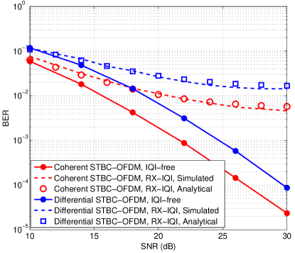
Figure 1: Comparison of Analytical and Measured BER performance of the DSTBC-OFDM system under RX-IQI.

The performance of RX-IQI compensation is presented in Fig. 2. We evaluate the performance in both fast-fading and slow-fading channels. Fig. 2 shows that our proposed compensation algorithm effectively mitigates RX-IQI. A performance degradation is observed in the fast-fading channel even without IQI since the fast-varying channel does not satisfy the quasi-static property assumed by differential STBC. However, since the RX-IQI compensation matrix does not change with the channel, the compensation is effective in both slow and fast fading channel scenarios and the degradation caused by RX-IQI is almost eliminated.

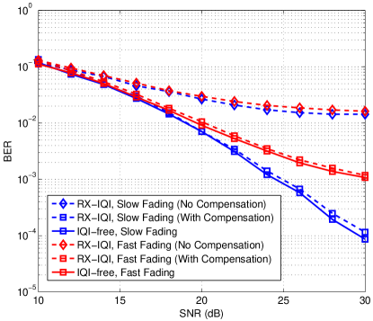
Figure 2: BER performance of the DSTBC-OFDM system under RX-IQI in slow and fast fading channels

VI Conclusion

In this paper, we analyzed the impact of RX-IQI on the BER of DSTBC-OFDM systems. We quantified analytically the BER floor due to RX-IQI and demonstrated its accuracy by simulations. In addition, a compensation scheme for DSTBC-OFDM system is proposed and demonstrated to effectively mitigate the performance degradation caused by RX-IQI in both slow and fast fading channels.

References

• [1] S. N. Diggavi, N. Al-Dhahir, A. Stamoulis, and A. R. Calderbank, “Great expectations: The value of spatial diversity in wireless networks,” Proceedings of the IEEE, vol. 92, no. 2, pp. 219–270, Feb. 2004.
• [2] V. Tarokh and H. Jafarkhani, “A differential detection scheme for transmit diversity,” IEEE Journal on Selected Areas in Communications, vol. 18, no. 7, pp. 1169–1174, Jul. 2000.
• [3] S. N. Diggavi, N. Al-Dhahir, A. Stamoulis, and A. R. Calderbank, “Differential space-time coding for frequency-selective channels,” IEEE Communications Letters, vol. 6, no. 6, pp. 253–255, Jun. 2002.
• [4] S. Lu and N. Al-Dhahir, “Coherent and differential ICI cancellation for mobile OFDM with application to DVB-H,” IEEE Transactions on Wireless Communications, vol. 7, no. 11, pp. 4110 – 4116, Dec. 2008.
• [5] B. L. Hughes, “Differential space-time modulation,” IEEE Transactions on Information Theory, vol. 46, no. 7, pp. 2567–2578, Nov. 2000.
• [6] A. Tarighat, R. Bagheri, and A. H. Sayed, “Compensation schemes and performance analysis of IQ imbalances in OFDM receivers,” IEEE Transactions on Signal Processing, vol. 53, no. 8, pp. 3257–3268, Aug. 2005.
• [7] A. Tarighat and A. H. Sayed, “Joint compensation of transmitter and receiver impairments in OFDM systems,” IEEE Transactions on Wireless Communications, vol. 6, no. 1, pp. 240–247, Jan. 2007.
• [8] B. Narasimhan, S. Narayanan, H. Minn, and N. Al-Dhahir, “Reduced-complexity baseband compensation of joint Tx/Rx I/Q imbalance in mobile MIMO-OFDM,” IEEE Transactions on Wireless Communications, vol. 9, no. 5, pp. 1720–1728, May 2010.
• [9] M. Marey, M. Samir, and M. H. Ahmed, “Joint estimation of transmitter and receiver IQ imbalance with ML detection for Alamouti OFDM systems,” IEEE Transactions on Vehicular Technology, vol. 62, no. 6, pp. 2847–2853, Jul. 2013.
• [10] D. Tandur and M. Moonen, “STBC MIMO OFDM systems with implementation impairments,” in Proc.IEEE Vehicular Technology Conference (VTC-Fall ’08), Sept. 2008, pp. 1–5.
• [11] Y. Zou, M. Valkama, and M. Renfors, “Performance analysis of space-time coded MIMO-OFDM systems under I/Q imbalance,” in Proc. IEEE International Conference on Acoustics, Speech and Signal Processing (ICASSP ’07), vol. 3, Apr. 2007, pp. 341–344.
• [12] L. Anttila, M. Valkama, and M. Renfors, “Circularity-based I/Q imbalance compensation in wideband direct-conversion receivers,” IEEE Transactions on Vehicular Technology, vol. 57, no. 4, pp. 2099–2113, Jul. 2008.
• [13] S. M. Alamouti, “A simple transmit diversity technique for wireless communications,” IEEE Journal on Selected Areas in Communications, vol. 16, no. 8, pp. 1451–1458, Oct. 1998.
• [14] M. Torabi, S. Aïssa, and M. R. Soleymani, “On the BER performance of space-frequency block coded OFDM systems in fading MIMO channels,” IEEE Transactions on Wireless Communications, vol. 6, no. 4, pp. 1366–1373, Apr. 2007.
• [15] M. J. S. Morris H. DeGroot, Probability and Statistics (4th Edition).   Addison-Wesley, 2010.
• [16] C. Geng, H. Sun, and S. A. Jafar, “On the optimality of treating interference as noise: General message sets,” IEEE Transaction on Information Theory, vol. 61, no. 7, pp. 3722–3736, Jul. 2015.
• [17] B. Narasimhan, S. Narayanan, N. Al-Dhahir, and H. Minn, “Digital baseband compensation of joint TX/RX frequency-dependent I/Q imbalance in mobile MIMO-OFDM transceivers,” in Proc. Annual Conference on Information Sciences and Systems (CISS ’09), Mar. 2009, pp. 545–550.