Abstract

Limit shape and fluctuations for exactly solvable inhomogeneous corner growth models

We study a class of corner growth models in which the weights are either all exponentially or all geometrically distributed. The parameter of the distribution at site $(i,j)$ is $a_{i}+b_{j}$ in the exponential case and $a_{i}b_{j}$ in the geometric case, where $(a_{i})_{i\geq 1}$ and $(b_{j})_{j\geq 1}$ are themselves drawn randomly at the outset from ergodic distributions. These models are inhomogeneous generalizations of the much studied exactly solvable models in which the parameters are the same for all sites. Our motivation is to understand how inhomogeneity influences the limit shape and the corresponding limit fluctuations. We obtain a simple variational formula for the shape function and prove that it is strictly concave inside a cone (possibly the entire quadrant) but is linear outside. This is in contrast with the situation in the models with i.i.d. weights in which the shape function is expected to be strictly concave under mild assumptions. For the directions inside the cone, we show that the limit fluctuations are governed by the Tracy-Widom GUE distribution and derive bounds for the deviations of the last-passage times above the shape function. To obtain the shape result, we couple the model with an explicit family of stationary versions of it. For the fluctuation and large deviation results, we perform steepest-descent analysis on an available Fredholm determinant formula for the one-point distribution of the last-passage time. We also develop a detailed appendix on the steepest-descent curves of harmonic functions of two real variables and approximate the contour integral of an arbitrary meromorphic function along such curves. This material can facilitate the steepest-descent arguments in the treatments of other related models as well.

Chapter 1 Introduction

1.1 The corner growth model

Stochastic models of planar growth have a long history in probabilistic research, dating at least as far back as the Eden model [16] and the more general Richardson models [39]. One can interpret these models as describing the spread of an infection in a tissue of cells over time. Each cell becomes susceptible to the infection under certain deterministic conditions such as the presence of at least one infected neighbor. Individual cells vary in resilience against the infection; therefore, the time period between the beginning of the susceptible state and the infected state for each cell is assumed random.

Despite the randomness in the dynamics, the set of infected cells can look like a deterministic limit shape after a long time. The first rigorous result of this sort is perhaps due to D. Richardson [39]. It has been of interest to understand when a limit shape exists and identify its features. Proceeding further, one can also inquire about the fluctuations around the limit shape. Satisfactory progress on these problems has been limited to specific rules of growth and the probability distributions governing the randomness.

The topic of this work is one of the most studied stochastic growth models known as the corner growth model, see [35], [45], [46]. The model is intimately connected to various other important models including the directed random polymer, directed last-passage percolation, M/M/1 queues in series and the totally asymmetric simple exclusion process (TASEP). Certain special cases of the model are known to be exactly solvable in the sense that rather precise analysis can be carried out. For these cases (the classical examples of which will be described below), it is known that the model is a member of the conjectural KPZ (Kardar-Parisi-Zhang) universality class, a large collection of statistical models that are expected to share certain universal behavior. For example, it is predicted that the scaling exponent of the fluctuations of the interesting observables in the KPZ-models is $1/3$ and the limit fluctuations are given by a Tracy-Widom distribution, see the survey [12] and the references therein.

In this introductory section, we define the general version of the corner growth model and allude to its connections to various other models. We also state the well-known shape and fluctuation results that our work extends. A brief guide to the organization of the material in the remainder of the text follows. Section 1.2 defines precisely the class of corner growth models treated here. Section 1.3 includes a discussion of our main results. Section 1.4 is a short survey of related works from the literature. The proof of the limit shape result is given in Chapter 2, which is taken from [19]. Chapter 3 is an exposition of the exact one-point distribution formula for the last-passage and appeared earlier in [17]. Chapter 4 proves the fluctuation and large deviation results.

We now define the corner growth model. Represent a set of sites with $\operatorname{\mathbb{N}}^{2}$, where $\operatorname{\mathbb{N}}=\{1,2,3,\dotsc\}$. At the outset, each site $(i,j)\in\operatorname{\mathbb{N}}$ is assigned a weight $W(i,j)$, a randomly chosen nonnegative real number. In the general version of the model, the joint distribution $\operatorname{\mathbf{P}}$ of the weights $\{W(i,j):i,j\in\operatorname{\mathbb{N}}\}$ is an arbitrary (Borel) probability measure on $\operatorname{\mathbb{R}}_{+}^{\operatorname{\mathbb{N}}^{2}}$. The dynamics begins with all sites initially colored white at time $t=0$. Each site $(i,j)$ changes color to red permanently after $W(i,j)$ amount of time has elapsed since the first time both of the following conditions hold.

• If $i>1$ then $(i-1,j)$ is red.

• If $j>1$ then $(i,j-1)$ is red.

To relate to the story of an epidemic, imagine the sites as cells, white cells as healthy, red cells as infected and the weights as the resilience of the cells. A healthy cell is susceptible to the infection if its left and bottom neighbors (if they exist) are already infected. Hence, the epidemic starts out from the corner $(1,1)$ and spreads to the entire quadrant $\operatorname{\mathbb{N}}^{2}$ over time.

For each $(i,j)\in\operatorname{\mathbb{N}}^{2}$, let $G(i,j)$ denote the time when the site $(i,j)$ becomes red. Let $\operatorname{\mathcal{S}}_{t}$ denote the set of red sites at time $t\geq 0$ i.e.

$$\operatorname{\mathcal{S}}_{t}=\{(i,j)\in\operatorname{\mathbb{N}}^{2}:G(i,j)\leq t\}\quad\text{ for }t\geq 0.$$ (1.1.1)

To understand the limit shape of red sites, it is helpful to study the random variables $\{G(i,j):i,j\in\operatorname{\mathbb{N}}\}$. The growth rule above translates to the recursion

$$G(i,j) =G(i-1,j)\vee G(i,j-1)+W(i,j)$$ (1.1.2)

$$G(i,0) =G(0,j)=0$$ (1.1.3)

for $i,j\in\operatorname{\mathbb{N}}$. One can also picture the preceding recursion as a sequence of servers labeled with $i\in\operatorname{\mathbb{N}}$ serving a sequence of customers labeled with $j\in\operatorname{\mathbb{N}}$ [24]. Each server delivers service to the customers one by one in the order the customers arrive. Each customer arrives the system by joining the queue at server $1$. For each $i,j\in\operatorname{\mathbb{N}}$, the amount of time server $i$ needs for the service of customer $j$ is $W(i,j)$. When this service is completed, customer $j$ immediately departs and joins the queue at the server $i+1$, and the server $i$ becomes available for the next customer $j+1$. We will not take advantage of this viewpoint here and refer the interested reader to [35] and [46].

Another equivalent description of the last-passage times is in terms of directed paths. A directed path $\pi$ is a finite sequence $\pi=((i_{k},j_{k}))_{1\leq k\leq l}$ in $\operatorname{\mathbb{Z}}^{2}$ such that

$$(i_{k+1}-i_{k},j_{k+1}-j_{k})\in\{(1,0),(0,1)\}\quad\text{ for }1\leq k<l.$$

We say that $\pi$ is from $(u,v)\in\operatorname{\mathbb{Z}}^{2}$ to $(u^{\prime},v^{\prime})\in\operatorname{\mathbb{Z}}^{2}$ if $(i_{1},j_{1})=(u,v)$ and $(i_{l},j_{l})=(u^{\prime},v^{\prime})$. See Figure 1. We have

$$G(m,n)=\max_{\pi\in\Pi_{1,1,m,n}}\sum\limits_{(i,j)\in\pi}W(i,j)\quad\text{ for }m,n\in\operatorname{\mathbb{N}},$$ (1.1.4)

where $\Pi_{u,v,u^{\prime},v^{\prime}}$ denotes the set of all directed paths from $(u,v)$ to $(u^{\prime},v^{\prime})$. Hence, $\{G(i,j):i,j\in\operatorname{\mathbb{N}}\}$ are exactly the last-passage time variables of the directed last-passage percolation. This connection seems to have been first observed in [36].

Figure 1: A directed path (red) from $(1,1)$ to $(m,n)=(6,6)$. Blue dots indicate sites.

The first limit shape result for the corner growth model appeared in the pioneering work of H. Rost [40], which studied the totally asymmetric simple exclusion process (TASEP). This is a fundamental interacting particle system that can be viewed as a toy model for single-lane traffic. In the version relevant to the present discussion, we consider particles labeled with $i\in\operatorname{\mathbb{N}}$ residing at the sites of $\operatorname{\mathbb{Z}}$. Let $\sigma(i,t)\in\operatorname{\mathbb{Z}}$ denote the position of particle $i\in\operatorname{\mathbb{N}}$ at time $t\geq 0$. Impose the jam (step) initial condition i.e. $\sigma(i,0)=-i$ for $i\in\operatorname{\mathbb{N}}$. At the outset particles are equipped with independent Poisson clocks with rate $\lambda>0$. The positions of the particles are updated as follows. A particle currently at site $j\in\operatorname{\mathbb{Z}}$ jumps to $j+1$ when its clock rings provided that there is no particle at $j+1$. This exclusion constraint, which disallows presence of two particles at the same site, is the interaction between otherwise independently moving particles. As explained, for example, in [46, p 5], the distribution of $\{(i,j)\in\operatorname{\mathbb{N}}^{2}:\sigma(i,t)\leq i+j\}$ is the same as the distribution of $\operatorname{\mathcal{S}}_{t}$ in the exponential model, the corner growth model with i.i.d. weights such that

$$\operatorname{\mathbf{P}}(W(i,j)\geq x)=e^{-\lambda x}\text{ for }i,j\in\operatorname{\mathbb{N}}\text{ and }x\geq 0.$$ (1.1.5)

As a corollary of his results for TASEP, Rost obtained that

$$\lim\limits_{n\rightarrow\infty}\frac{G(\operatorname{\lfloor}ns\operatorname{\rfloor},\operatorname{\lfloor}nt\operatorname{\rfloor})}{n}=\frac{(\sqrt{s}+\sqrt{t})^{2}}{\lambda}\quad\text{ for }s,t>0\quad\operatorname{\mathbf{P}}\text{-a.s.}$$ (1.1.6)

He also showed that the rescaled set of red sites

$$\frac{1}{t}\operatorname{\mathcal{S}}_{t}=\{(i,j)\in\operatorname{\mathbb{N}}^{2}:G(\operatorname{\lfloor}ti\operatorname{\rfloor},\operatorname{\lfloor}tj\operatorname{\rfloor})\leq t\}$$ (1.1.7)

converges $\operatorname{\mathbf{P}}$-a.s. as $t\rightarrow\infty$ to the parabolic region $\{s,t\in\operatorname{\mathbb{R}}_{+}:\sqrt{s}+\sqrt{t}\leq\sqrt{\lambda}\}$ in a certain sense.

There is also a discrete-time version of TASEP in which time variable $t\in\operatorname{\mathbb{Z}}_{+}$. Particles now carry independent coins with tails probability $q\in(0,1)$. For $i\in\operatorname{\mathbb{N}}$ and $t\in\operatorname{\mathbb{Z}}_{+}$, the position of particle $i$ at time $t+1$ is determined from the particle configuration at time $t$ as follows. Particle $i$ flips its coin at time $t$. If heads comes up and the position $\sigma(i,t)+1$ is empty then $\sigma(i,t+1)=\sigma(i,t)+1$; otherwise, $\sigma(i,t+1)=\sigma(i,t)$. The discrete-time TASEP with step initial condition is equivalent to the corner growth model in which the weights are i.i.d. and

$$P(W(i,j)\geq k)=q^{k}\quad\text{ for }i,j\in\operatorname{\mathbb{N}}\text{ and }k\in\operatorname{\mathbb{Z}}_{+}.$$ (1.1.8)

For this geometric model, the limit shape has also been computed.

$$\lim\limits_{n\rightarrow\infty}\frac{G(\operatorname{\lfloor}ns\operatorname{\rfloor},\operatorname{\lfloor}nt\operatorname{\rfloor})}{n}=\frac{q}{1-q}(s+t)+\frac{2\sqrt{q}}{1-q}\sqrt{st}\quad\text{ for }s,t>0\quad\operatorname{\mathbf{P}}\text{-a.s., }$$ (1.1.9)

[11], [31], [44].

The limit fluctuations corresponding to (1.1.6) and (1.1.8) were derived in the breakthrough work of K. Johansson [27, Theorem 1.2]. For the geometric model, for $r>0$,

$$\lim\limits_{n\rightarrow\infty}\operatorname{\mathbf{P}}(G(\operatorname{\lfloor}nr\operatorname{\rfloor},n)\leq n\gamma(r)+n^{1/3}\sigma(r)s)=F_{\operatorname{GUE}}(s)\quad\text{ for }s\in\operatorname{\mathbb{R}},$$ (1.1.10)

where

$$\gamma(r) =\frac{q(1+r)+2\sqrt{qr}}{1-q},$$ (1.1.11)

$$\sigma(r) =\frac{1}{1-q}\left(\frac{q}{r}\right)^{1/6}(\sqrt{q}+\sqrt{r})^{2/3}(1+\sqrt{qr})^{2/3}$$ (1.1.12)

and $F_{\operatorname{GUE}}$ denotes the c.d.f. of the Tracy-Widom GUE distribution defined in Section A.1. For the exponential model, (1.1.10) is also true with different explicit constants $\gamma(r)$ and $\sigma(r)$, [27, Theorem 1.6].

Precise description of the limit shape and limit fluctuations such as (1.1.9) and (1.1.10) for the corner growth model is presently only possible for the exponential and geometric models, and their derivatives (an example of which is treated in this work). It is expected that the model exhibit certain features that are universal, which are there irrespective of the underlying weight distribution. For example, at least when $\operatorname{\mathbf{P}}$ is i.i.d. and satisfies mild conditions, the shape function is expected to be strictly concave and differentiable. The limit fluctuations should be governed by the Tracy-Widom GUE distribution as in (1.1.10).

1.2 Exponential and geometric models with inhomogeneous parameters

The class of models we study are inhomogeneous generalizations of the exponential and geometric models. The parameters $\lambda$ and $q$ themselves will now be randomly chosen for each site at the outset and then kept fixed throughout the dynamics. It turns out that, for certain choices of the parameter distributions, the resulting models are still amenable to precise analysis. Taking advantage of this situation, we find the analogues of H.Rost’s limit shape result (1.1.6) and K.Johansson’s fluctuation result (1.1.10) for these inhomogeneous models. The next section discusses in detail the contribution of the present work. Here, we provide a precise description of the inhomogeneous exponential and geometric models and allude to their aspects that lead to exact solvability.

For concreteness, let us construct the sample space of the weights as $\operatorname{\mathbb{R}}_{+}^{\operatorname{\mathbb{N}}^{2}}$ equipped with the Borel $\sigma$-algebra. Define $W(i,j)$ as the projection map $\operatorname{\mathbb{R}}_{+}^{\operatorname{\mathbb{N}}^{2}}\rightarrow\operatorname{\mathbb{R}}_{+}$ onto coordinate $(i,j)$ for $i,j\in\operatorname{\mathbb{N}}$. Let $\operatorname{\mathbf{a}}=(a_{n})_{n\in\operatorname{\mathbb{N}}}$ and $\operatorname{\mathbf{b}}=(b_{n})_{n\in\operatorname{\mathbb{N}}}$ be stationary random sequences with terms in $(0,\infty)$ for the exponential model and in $(0,1)$ for the geometric model. For the shape results, we will assume that the pair $(\operatorname{\mathbf{a}},\operatorname{\mathbf{b}})$ is totally ergodic with respect to the shifts $(a_{n},b_{n})\mapsto(a_{n+k},b_{n+l})$ for $k,l\in\operatorname{\mathbb{N}}$, see Section 2.1. As an example, take $\operatorname{\mathbf{a}}$ and $\operatorname{\mathbf{b}}$ as independent i.i.d. sequences. For the fluctuation results, the total ergodicity assumption is weakened to ergodicity of $\operatorname{\mathbf{a}}$ and $\operatorname{\mathbf{b}}$ (i.e. these sequences are each ergodic and no assumption is made on their joint distribution). Suppose that, given $(\operatorname{\mathbf{a}},\operatorname{\mathbf{b}})$, the weights $\{W(i,j):i,j\in\operatorname{\mathbb{N}}\}$ are conditionally independent and the joint conditional distribution $\operatorname{\mathbf{P}}_{\operatorname{\mathbf{a}},\operatorname{\mathbf{b}}}$ of the weights are given by

$$\operatorname{\mathbf{P}}_{\operatorname{\mathbf{a}},\operatorname{\mathbf{b}}}(W(i,j)\geq x)=e^{-(a_{i}+b_{j})x}\quad\text{ for }i,j\in\operatorname{\mathbb{N}}\text{ and }x\geq 0$$ (1.2.1)

for the exponential model and

$$\operatorname{\mathbf{P}}_{\operatorname{\mathbf{a}},\operatorname{\mathbf{b}}}(W(i,j)\geq k)=a_{i}^{k}b_{j}^{k}\quad\text{ for }i,j\in\operatorname{\mathbb{N}}\text{ and }k\in\operatorname{\mathbb{Z}}_{+}$$ (1.2.2)

for the geometric model.

Let $\operatorname{\mathbb{P}}$ denote the (unconditional) joint distribution of the weights. Thus, $\operatorname{\mathbb{P}}(B)=\int\operatorname{\mathbf{P}}_{\operatorname{\mathbf{a}},\operatorname{\mathbf{b}}}(B)\mu(\mathrm{d}\operatorname{\mathbf{a}},\mathrm{d}\operatorname{\mathbf{b}})$ for any Borel set $B\subset\operatorname{\mathbb{R}}_{+}^{\operatorname{\mathbb{N}}^{2}}$, where $\mu$ is the joint distribution of $(\operatorname{\mathbf{a}},\operatorname{\mathbf{b}})$. By stationarity of $\operatorname{\mathbf{a}}$ and $\operatorname{\mathbf{b}}$, the weights are identically distributed under $\operatorname{\mathbb{P}}$. However, there are nontrivial correlations among the weights since $W(i,j)$ and $W(i^{\prime},j^{\prime})$ are, in general, not independent under $\operatorname{\mathbb{P}}$ if $i=i^{\prime}$ or $j=j^{\prime}$.

We mention the key features that render these inhomogeneous models well-suited for analysis. For the limit shape result, we exploit an explicit one-parameter family of product probability measures $\operatorname{\mathbf{P}}_{\operatorname{\mathbf{a}},\operatorname{\mathbf{b}}}^{z}$ on the extended sample space $\operatorname{\mathbb{R}}_{+}^{\operatorname{\mathbb{Z}}_{+}^{2}}$ that project to $\operatorname{\mathbf{P}}_{\operatorname{\mathbf{a}},\operatorname{\mathbf{b}}}$ on $\operatorname{\mathbb{R}}_{+}^{\operatorname{\mathbb{N}}^{2}}$, see (2.4.2) and (2.4.3) below. These measures satisfy a useful stationarity property (Proposition 2.4.1) sometimes referred to as the Burke property that enables exact computations. This approach was introduced in [44]. For the fluctuation results, our starting point is that the probabilities $\operatorname{\mathbf{P}}_{\operatorname{\mathbf{a}},\operatorname{\mathbf{b}}}(G(m,n)\leq k)$ can be represented as a Fredholm determinant with a tractable kernel [28]. Derivation of this formula is discussed at length in Chapter 3.

1.3 Main results

Our first result is the identification of the shape function in terms of a one-dimensional variational problem. Some notation is needed to state it. Let $\alpha$ and $\beta$ denote the distributions of $a_{1}$ and $b_{1}$, respectively. (By stationarity of $\operatorname{\mathbf{a}}$ and $\operatorname{\mathbf{b}}$, $a_{n}$ and $b_{n}$ are distributed as $\alpha$ and $\beta$, respectively, for $n\in\operatorname{\mathbb{N}}$). For a Borel measure $\eta$ on $\operatorname{\mathbb{R}}$, let $\underaccent{\bar}{\eta}$ and $\bar{\eta}$ denote the left and right endpoints of the support of $\eta$ (the complement of the largest open $\eta$-null set). Extend $\alpha$ and $\beta$ as Borel probability measures to $\operatorname{\mathbb{R}}$. Then the support of $\alpha$ and $\beta$ are contained in $[0,\infty)$ with $\alpha(\{0\})=\beta(\{0\})=0$ for the exponential model, and the supports are contained in $[0,1]$ with $\alpha(\{0,1\})=\beta(\{0,1\})=0$ for the geometric model. Also, $\underaccent{\bar}{\alpha}$ and $\bar{\alpha}$ equal, respectively, the essential infimum and the essential supremum of $a_{1}$. Similarly for $\beta$.

The shape function is given by

$$g(s,t)=\inf\limits_{z\in[-\underaccent{\bar}{\alpha},\underaccent{\bar}{\beta}]}\left\{s\int_{0}^{\infty}\frac{\alpha(\mathrm{d}a)}{a+z}+t\int_{0}^{\infty}\frac{\beta(\mathrm{d}b)}{b-z}\right\}\quad\text{ for }s,t>0$$ (1.3.1)

for the exponential model. This will be restated as Theorems 2.2.1 and 2.2.2. The infimum above can be computed explicitly when $\alpha$ and $\beta$ are uniform measures. For example, if $\alpha$ and $\beta$ are uniform on the interval $[1/2,3/2]$ then

$$g(s,t)=s\log\bigg{(}\frac{t+7s+\sqrt{(s+t)^{2}+12st}}{4s}\bigg{)}+t\log\bigg{(}\frac{s+7t+\sqrt{(s+t)^{2}+12st}}{4t}\bigg{)}.$$ (1.3.2)

for $s,t>0$. For this choice of $\alpha$ and $\beta$, Figure 2 below illustrates the limit shape result when $\operatorname{\mathbf{a}}$ and $\operatorname{\mathbf{b}}$ are i.i.d. sequences. If $\underaccent{\bar}{\alpha}=\underaccent{\bar}{\beta}=0$ then (1.3.1) reduces to

$$g(s,t)=s\int_{0}^{\infty}\frac{\alpha(\mathrm{d}a)}{a}+t\int_{0}^{\infty}\frac{\beta(\mathrm{d}b)}{b}\quad\text{ for }s,t>0.$$ (1.3.3)

In particular, $g$ is a linear function if the above integrals are both finite, and is identically infinite otherwise. For $\underaccent{\bar}{\alpha}+\underaccent{\bar}{\beta}>0$, the following properties of $g$ can be derived from (1.3.1), see Corollary 2.2.3. There are critical values $0\leq c_{1}<c_{2}\leq\infty$ determined by $\alpha$ and $\beta$ such that, as a function of $(s,t)$, $g$ is strictly concave for $c_{1}<s/t<c_{2}$ but is linear for $s/t\leq c_{1}$ or $s/t\geq c_{2}$. We have $c_{1}=0$ if and only if $\int_{0}^{\infty}(a-\underaccent{\bar}{\alpha})^{-2}\alpha(\mathrm{d}a)=\infty$, and $c_{2}=\infty$ if and only if $\int_{0}^{\infty}(b-\underaccent{\bar}{\beta})^{-2}\beta(\mathrm{d}b)=\infty$. Hence, the linear regions of $g$ can be empty as is the case in (1.3.2). Also, $g$ is $\operatorname{\mathcal{C}}^{1}$. Consequently, the graph of $g$ does not have a sharp corner along the critical lines $s/t=c_{1}$ and $s/t=c_{2}$. These features are depicted on the level curve $g(s,t)=1$ for a particular choice of $\alpha$ and $\beta$ in Figure 3 below.

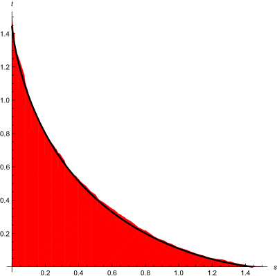
Figure 2: The output of a simulation of the inhomogeneous exponential model up to time $t=2000$. The sequences $\operatorname{\mathbf{a}}$ and $\operatorname{\mathbf{b}}$ are i.i.d, and $\alpha$ and $\beta$ are uniform on $[1/2,3/2]$. The red region is the rescaled set of red sites $t^{-1}\operatorname{\mathcal{S}}_{t}$ when $t=2000$. The black curve is the level set $g(s,t)=1$ for (1.3.2).

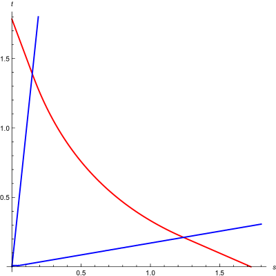
Figure 3: The level curve $g(s,t)=1$ and the rays $s/t=c_{1}=(-8+12\log 2)/3\approx 0.105922$ and $s/t=c_{2}=4/(9-12\log 2)\approx 5.863092$ for (1.3.1) when $\alpha(\mathrm{d}a)=\operatorname{\mathbf{1}}_{\{0\leq a\leq 1\}}3a^{2}\mathrm{d}a$ and $\beta(\mathrm{d}b)=\operatorname{\mathbf{1}}_{\{1\leq b\leq 2\}}4(b-1)^{3}\mathrm{d}b$.

For the geometric model, we have similar results for the limit shape. The analogue of (1.3.1) is stated as Theorems 2.2.6 and 2.2.7, and a closed form formula similar to (1.3.2) can be derived when $\alpha$ and $\beta$ have densities proportional to $x\mapsto 1/x$. If $\bar{\alpha}=\bar{\beta}=1$ then $g$ is linear or infinite. If $\bar{\alpha}\bar{\beta}<1$ then $g$ is strictly concave inside the region $c_{1}<s/t<c_{2}$ and linear outside for some constants $0\leq c_{1}<c_{2}\leq\infty$ as exemplified in Figure 3. Now $c_{1}=0$ if and only if $\int_{0}^{1}(\bar{\alpha}-a)^{-2}\alpha(\mathrm{d}a)=\infty$, and $c_{2}=\infty$ if and only if $\int_{0}^{1}(\bar{\beta}-b)^{-2}\beta(\mathrm{d}b)=\infty$.

The next set of results concerns the fluctuations around the limit shape with respect to $\operatorname{\mathbf{P}}_{\operatorname{\mathbf{a}},\operatorname{\mathbf{b}}}$ for a.e. realization of $\operatorname{\mathbf{a}}$ and $\operatorname{\mathbf{b}}$. At present, we only study the fluctuations in the strictly concave region $c_{1}<s/t<c_{2}$ of the geometric model. We do not expect difficulty in repeating the analysis here for the strictly concave region of the exponential model. However, the treatment of the linear regions (in both models) seems to require significant further work.

Our first result bounds the right tail deviations of the last-passage times i.e. deviations above the shape function. Fix $r\in(c_{1},c_{2})$ and set $\gamma(r)=g(r,1)$. Then, for a.e. $(\operatorname{\mathbf{a}},\operatorname{\mathbf{b}})$, there are deterministic constants $C,c>0$, $n_{0}=n_{0}^{\operatorname{\mathbf{a}},\operatorname{\mathbf{b}}}\in\operatorname{\mathbb{N}}$ and a sequence $\gamma_{n}=\gamma_{n}^{\operatorname{\mathbf{a}},\operatorname{\mathbf{b}}}$ converging a.s. to $\gamma$ such that

$$\operatorname{\mathbf{P}}_{\operatorname{\mathbf{a}},\operatorname{\mathbf{b}}}(G(\operatorname{\lfloor}nr\operatorname{\rfloor},n)\geq n\gamma_{n}+ns) \leq Ce^{-cn(s^{3/2}\wedge s)}$$ (1.3.4)

for $s\geq 0$ and $n\geq n_{0}$. In particular, up to a constant, the decay rate of the exponential bound is $s^{3/2}$ and $s$ for small and large values of $s$, respectively. In (1.3.4), the transition occurs at $s=1$ although this point can be moved to any positive number by altering the constants $C,c$. We state (1.3.4) in a slightly more general form as Theorem 4.2.1. When $\alpha$ and $\beta$ are delta masses then $\operatorname{\mathbf{a}}$ and $\operatorname{\mathbf{b}}$ are constant sequences a.s. In this case, we also have $\gamma_{n}=\gamma$ for $n\in\operatorname{\mathbb{N}}$, and (1.3.4) then becomes

$$\operatorname{\mathbf{P}}(G(\operatorname{\lfloor}nr\operatorname{\rfloor},n)\geq n\gamma+ns)\leq Ce^{-cn(s^{3/2}\wedge s)}$$ (1.3.5)

for $s\geq 0$ and $n\geq n_{0}$ for some constants $C,c>0$ and $n_{0}\in\operatorname{\mathbb{N}}$, where $\operatorname{\mathbf{P}}$ is the i.i.d. measure given by (1.1.8) with $q=a_{1}b_{1}$. We point out that (1.3.5) is not new. Although not recorded explicitly, it can be deduced from [27, Theorem 2.2, (2.17), (2.21)-(2.23), Corollary 2.4]. For the exponential model, (1.3.5) (for small values of $s$) was previously pointed out in [42, p. 622]. Our proof of (1.3.5) is quite different; it comes from a steepest-descent analysis and does not involve computation of the right tail large deviation rate function.

We also mention that (1.3.5) improves the following right tail bound that recently appeared in [13, Lemma 2.2]. There exists $M,\delta,c>0$ such that

$$\operatorname{\mathbf{P}}(G(\operatorname{\lfloor}nr\operatorname{\rfloor},n)\geq n\gamma+n^{1/3}x)\leq e^{-cx}$$ (1.3.6)

for $M\leq x\leq\delta n^{1/3}$. In contrast, setting $s=n^{-2/3}x$ in (1.3.5) yields

$$\operatorname{\mathbf{P}}(G(\operatorname{\lfloor}nr\operatorname{\rfloor},n)\geq n\gamma+n^{1/3}x)\leq Ce^{-c(x^{3/2}\wedge(n^{1/3}x))}$$ (1.3.7)

for $x\geq 0$ and $n\geq n_{0}$. In the regime $M\leq x\leq\delta n^{1/3}$ (where $M$ is a large constant), we have $x\leq x^{3/2}\leq n^{1/3}x$. Thus,

$$\operatorname{\mathbf{P}}(G(\operatorname{\lfloor}nr\operatorname{\rfloor},n)\geq n\gamma+n^{1/3}x)\leq Ce^{-cx^{3/2}}\leq e^{-c^{\prime}x^{3/2}}$$ (1.3.8)

for another constant $c^{\prime}>0$, and (1.3.6) follows.

Another result we wish to highlight here is that the quenched limit fluctuations of the last-passage times in the stricly concave region is governed by the Tracy-Widom GUE distribution denoted $F_{\operatorname{GUE}}$ below (see Section A.1 for its definition). More precisely,

$$\lim_{n\rightarrow\infty}\operatorname{\mathbf{P}}_{\operatorname{\mathbf{a}},\operatorname{\mathbf{b}}}(G(\operatorname{\lfloor}nr\operatorname{\rfloor},n)\leq n\gamma_{n}+n^{1/3}\sigma_{n}s)=F_{\operatorname{GUE}}(s)\quad\text{ for }s\in\operatorname{\mathbb{R}}$$ (1.3.9)

for a.e. $(\operatorname{\mathbf{a}},\operatorname{\mathbf{b}})$, where $\sigma_{n}$ is a sequence (depending on $\operatorname{\mathbf{a}},\operatorname{\mathbf{b}}$) converging to a deterministic quantity $\sigma>0$. This result is contained Theorem 4.2.13. Note that due to continuity of $F_{\operatorname{GUE}}$ and the monotonicity of the left-hand side in $s\in\operatorname{\mathbb{R}}$, (1.3.9) also holds if $\sigma_{n}$ is replaced with the limit value $\sigma$. We confirm via (1.3.9) that the inhomogeneous geometric model behaves as a KPZ class model in the strictly concave region. This was predicted in [20] on account of the expansion of the right tail rate functions and by analogy with a similar result of J.Gravner, C.Tracy and H.Widom [25, Theorem 3] for a related model known as Johansson-Seppäläinen model, which we elaborate on in the next section.

Since $\lim_{n\rightarrow\infty}\gamma_{n}=\gamma$, (1.3.9) also implies $n^{-1}G(\operatorname{\lfloor}nr\operatorname{\rfloor},n)=\gamma$ in $\operatorname{\mathbf{P}}_{\operatorname{\mathbf{a}},\operatorname{\mathbf{b}}}$-probability a.s under the weaker hypotheses that $\operatorname{\mathbf{a}}$ and $\operatorname{\mathbf{b}}$ are each ergodic rather than jointly totally ergodic. We expect that a.s convergence also holds but at present we only have $\limsup_{n\rightarrow\infty}n^{-1}G(\operatorname{\lfloor}nr\operatorname{\rfloor},n)\leq\gamma(r)$ a.s., which follows from the Borel-Cantelli lemma using (1.3.4). An exponential bound for the left tail deviations in the i.i.d. setting is known [4]. Obtaining the corresponding bound in the inhomogeneous setting is left for future work.

The main strategy to prove the fluctuation and large deviation bound comes from [25]. The distributions of the last-passage times admit a Fredholm determinant representation with an explicit kernel depending on finitely many terms from $\operatorname{\mathbf{a}}$ and $\operatorname{\mathbf{b}}$ [28]. This naturally leads to the consideration of the empirical distributions $\alpha_{n}$ and $\beta_{n}$ approximating $\alpha$ and $\beta$, respectively. The sequence $\gamma_{n}(r)$ is, in fact, precisely the shape function (1.3.1) computed with $(s,t)=(r,1)$ and using $\alpha_{\operatorname{\lfloor}nr\operatorname{\rfloor}}$ and $\beta_{n}$ in place of $\alpha$ and $\beta$, respectively. The analysis of the kernel involves use of the steepest-descent curves through the minimizer of the variational formula for $\gamma_{n}$. Since this minimizer is a saddle point of order $2$, the Airy kernel arises in the asymptotics. Because we work with infinitely many steepest-descent curves, sufficiently strong uniform control of these curves is needed for various steps in the argument. In our case, such a control is afforded by the ergodicity of $\operatorname{\mathbf{a}}$ and $\operatorname{\mathbf{b}}$.

This work also attempts to go beyond the purpose of deriving the Tracy-Widom limit for the inhomogeneous geometric model with various future applications in mind. In Section A.2, we provide a short and largely self-contained treatment of the steepest-descent curves of harmonic functions on $\operatorname{\mathbb{C}}$. These lemmas offer quantative bounds and help describe rigorously the local and global nature of the steepest-descent curves. In Section A.3, we approximate the contour integral of an arbitrary meromorphic function along the steepest-descent curve of its (approximate) logarithm. We present an application of this material in our derivation of the fluctuation results. Another immediate use in a work in progress is to compute the right tail rate function.

1.4 Literature review

We give a brief overview of the literature in relation to the present work. By (1.1.6) and (1.1.9), the shape functions of the exponential and geometric models satisfy

$$g(s,t)=m(s+t)+2\sqrt{\sigma^{2}st}\quad\text{ for }s,t>0,$$ (1.4.1)

where $m$ and $\sigma^{2}$ denote the common mean and the variance of the weights. Such explicit description of the shape function for all directions $(s,t)$ were not previously available for other weight distributions. Our variational characterization of the shape function furnishes new explicit formulas such as (1.3.2). J.Martin proved that, for i.i.d $\operatorname{\mathbf{P}}$ and assuming the weights have sufficiently light tail, (1.4.1) also holds up to an error of order $o(\sqrt{t})$ as $t\downarrow 0$. In particular, $g$ cannot be linear near the axes in contrast with the inhomogeneous setting where this is a real possibility, see Figure 3. For i.i.d. $\operatorname{\mathbf{P}}$, the linear regions can appear away from the axes. For example, if the weights are bounded and attain their maximum with probability larger than the critical probability for the oriented site percolation then $g(s,t)=s+t$ in a nontrivial cone [2], [15], [34]. Variational formulas characterizing $g$ have recently been derived for general i.i.d. weights with finite $2+\epsilon$ moments for some $\epsilon>0$ [23].

For the exponential model with i.i.d. $\operatorname{\mathbf{a}}$ and constant $\operatorname{\mathbf{b}}$, [47] obtained a variational description of $g$, which (1.3.1) includes as a special case. Asymptotics of $g$ near the axes are determined for more general $P$ in [33]. Their Theorem 2.4 can be deduced from (1.3.1) as well. Another direction of generalizing the exponential and geometric models is to choose the parameters at site $(i,j)$ as $\lambda=\Lambda(i/n,j/n)$ and $q=Q(i/n,j/n)$ for some deterministic functions $\Lambda$ and $Q$ that encode inhomogeneity. Then, under suitable conditions, $g$ can be characterized as the unique monotone viscosity solution of a certain Hamilton-Jacobi equation [10].

The fluctuation exponents for the exponential model were identified as KPZ exponents in [5]. The limit distribution for the rescaled last-passage times for the geometric and exponential models were proved to be the Tracy-Widom GUE distribution by K. Johansson in [27], see (1.1.10). [29] proved that suitably rescaled last-passage time process along the antidiagonal through $(n,n)$ converges to the Airy process, [29]. The measures $\operatorname{\mathbf{P}}_{\operatorname{\mathbf{a}},\operatorname{\mathbf{b}}}$ defined at (1.2.1) and (1.2.2) appeared earlier in [9] and [28], respectively, and is closely related to the Schur measures introduced in [37]. This connection leads to representations of the last-passage distributions in terms of Fredholm determinants with explicit kernels, see the exposition in Chapter 3 and the references therein. [9] considered $\operatorname{\mathbf{P}}_{\operatorname{\mathbf{a}},\operatorname{\mathbf{b}}}$ in (1.2.1) such that $(a_{i})_{i>k}$ and $(b_{j})_{j>l}$ are constant for fixed $k,l\in\operatorname{\mathbb{Z}}_{+}$ and identified the limit (in the sense of finite dimensional distributions) of the rescaled last-passage process (the parameters $a_{i},b_{j}$ for $i\in[k]$ and $j\in[l]$ are also rescaled suitably) along a certain line through $(nr,n)$ as a generalization of the extended Airy process. For similar setting with (1.2.2), [13] also determined the limit distribution of the rescaled last-passage times.

In [25], J.Gravner, C.Tracy and H.Widom studied a similarly inhomogeneous version of a variant of corner growth model known as oriented digital boiling or Johansson-Seppäläinen model introduced in [43]. The recursion (1.1.9) is now replaced with

$$G(i,j) =G(i-1,j)\vee(G(i,j-1)+W(i,j))\quad\text{ for }i,j\in\operatorname{\mathbb{N}}.$$ (1.4.2)

The weights $\{W(i,j):i,j\in\operatorname{\mathbb{N}}\}$ are independent and each $W(i,j)$ is Bernoulli-distributed with parameter $p_{j}$ for some ergodic sequence $(p_{j})_{j\in\operatorname{\mathbb{N}}}$. The shape function in this model has a constant, linear and strictly concave regions. A result from [25] is that, conditioned on the parameters $p_{j}$, suitably rescaled last-passage converge in distribution to the Tracy-Widom GUE distribution. (1.3.9) is the analogue of this result for the inhomogeneous geometric model and is derived through similar techniques.

1.5 Notation and conventions

Some standard notation that appears in this note are listed below.

Table 1: A guide to the notation

Notation	Definition
$\operatorname{\mathbb{N}}$	the set of natural numbers $\{1,2,3,\dotsc\}$
$\operatorname{\mathbb{Z}}_{+}$	the set of nonnegative integers $\{0,1,2,\dotsc\}$
$\operatorname{\mathbb{R}}_{+}$	the set of nonnegative real numbers
$\operatorname{\mathbb{H}}$	the set of $z\in\operatorname{\mathbb{C}}$ with $\Im z>0$.
$\mathbf{i}$	the imaginary unit
$[n]$	the set $\{1,\dotsc,n\}$ for $n\in\operatorname{\mathbb{N}}$
$a\vee b$	the maximum of $a,b\in\operatorname{\mathbb{R}}$
$a\wedge b$	the minimum of $a,b\in\operatorname{\mathbb{R}}$
$\hash S$	the number of elements in the set $S$
$\overline{z}$	the complex conjugate of $z\in\operatorname{\mathbb{C}}$
$\operatorname{\lfloor}x\operatorname{\rfloor}$	the largest integer less than or equal to $x\in\operatorname{\mathbb{R}}$
$\operatorname{\lceil}x\operatorname{\rceil}$	the least integer greater than or equal to $x\in\operatorname{\mathbb{R}}$
$|x|$	the Euclidean norm of $x\in\operatorname{\mathbb{R}}^{d}$
$\operatorname{D}(z,r)$	the (open) disk of radius $r$ centered at $z\in\operatorname{\mathbb{C}}$
$\operatorname{D}^{\prime}(z,r)$	the punctured disk $\operatorname{D}(z,r)\smallsetminus\{z\}$
$\operatorname{S}(z,r)$	the circle of radius $r$ centered at $z\in\operatorname{\mathbb{C}}$
$\operatorname{A}(z,r_{1},r_{2})$	the annulus $\{w\in\operatorname{\mathbb{C}}:r_{1}<|w-z|<r_{2}\}$
$[z,w]$	the oriented line segment from $z\in\operatorname{\mathbb{C}}$ to $w\in\operatorname{\mathbb{C}}$
$\delta_{i,j}$	the Kronecker delta function
$\bar{\eta}$	the right endpoint of the support of a Borel measure $\eta$ on $\operatorname{\mathbb{R}}$
$\underaccent{\bar}{\eta}$	the left endpoint of the support of a Borel measure $\eta$ on $\operatorname{\mathbb{R}}$
$x_{+}$	the positive part $\max\{x,0\}$ of $x\in\operatorname{\mathbb{R}}$.
$\operatorname{sgn}(x)$	the sign of $x\in\operatorname{\mathbb{R}}$. Equals $0$ if $x=0$ and $x/|x|$ otherwise.

The direction of $z\in\operatorname{\mathbb{C}}\smallsetminus\{0\}$ is defined as $z/|z|$. Adjectives increasing and decreasing are used in the strict sense. For convenience, we set $0^{0}=1$, $1/0=\infty$ and $1/\infty=0$.

In several computations, we will benefit from viewing $\operatorname{\mathbb{R}}^{2}$ as $\operatorname{\mathbb{C}}$ via the bijection $(x,y)\mapsto x+\mathbf{i}y$. Under this identification, we have a dot product on $\operatorname{\mathbb{C}}$ defined by $z\cdot w=\Re\{\overline{z}w\}$ for $z,w\in\operatorname{\mathbb{C}}$, which corresponds to the usual dot product on $\operatorname{\mathbb{R}}^{2}$.

Chapter 2 Limit Shape

2.1 Introduction

Refer to Section 1.2 for the descriptions of the exponential and geometric model. Let $\tau_{k}$ denote the shift map $(c_{n})_{n\in\operatorname{\mathbb{N}}}\mapsto(c_{n+k})_{n\in\operatorname{\mathbb{N}}}$ for $k\in\operatorname{\mathbb{Z}}_{+}$. We assume that the joint distribution $\mu$ of $(\operatorname{\mathbf{a}},\operatorname{\mathbf{b}})$ is totally ergodic with respect to the shifts $\tau_{k}\times\tau_{l}$ for $k,l\in\operatorname{\mathbb{N}}$. This means $\mu$ is separately ergodic under the map $\tau_{k}\times\tau_{l}$ for each $k,l\in\operatorname{\mathbb{N}}$.

Our results are formally stated in Section 2.2. We sketch the existence and the basic properties of $g$ in Section 2.3. We discuss stationary versions of the exponential and geometric models in Section 2.4. We prove (1.3.1) in Section 2.5.

2.2 Results

Let $\operatorname{E}$ denote the expectation under $\mu$ (the distribution of $(\operatorname{\mathbf{a}},\operatorname{\mathbf{b}})$). Recall that $a=a_{1}$ and $b=b_{1}$. It is convenient to break (1.3.1) into the next two theorems.

Theorem 2.2.1.

Suppose that $\underaccent{\bar}{\alpha}+\underaccent{\bar}{\beta}>0$ in the exponential model. Then

$$g(s,t)=\inf\limits_{z\in(-\underaccent{\bar}{\alpha},\underaccent{\bar}{\beta})}\ \left\{s\operatorname{E}\left[\frac{1}{a+z}\right]+t\operatorname{E}\left[\frac{1}{b-z}\right]\right\}\quad\text{ for }s,t>0.$$ (2.2.1)

Hence, $g$ depends on $(\operatorname{\mathbf{a}},\operatorname{\mathbf{b}})$ only through the marginal distributions $\alpha$ and $\beta$. Let us write $g^{\alpha,\beta}$ to indicate this. Replacing $z$ with $-z$ in (2.2.1) reveals that $g^{\alpha,\beta}(s,t)=g^{\beta,\alpha}(t,s)$ for $s,t>0$, which is expected due to the symmetric roles of $\operatorname{\mathbf{a}}$ and $\operatorname{\mathbf{b}}$ in the model. In particular, if $\alpha$ and $\beta$ are the same then $g(s,t)=g(t,s)$ for $s,t>0$. Also, (by dominated convergence) the infimum can be taken over $[-\underaccent{\bar}{\alpha},\underaccent{\bar}{\beta}]$ in (2.2.1). When $\underaccent{\bar}{\alpha}=\underaccent{\bar}{\beta}=0$, this interval degenerates to $\{0\}$ and we expect that $g(s,t)=s\operatorname{E}[1/a]+t\operatorname{E}[1/b]$ for $s,t>0$. Indeed, this is true.

Theorem 2.2.2.

Suppose that $\underaccent{\bar}{\alpha}=\underaccent{\bar}{\beta}=0$ in the exponential model. Then

$$g(s,t)=s\operatorname{E}\left[\frac{1}{a}\right]+t\operatorname{E}\left[\frac{1}{b}\right]\text{ for }s,t>0.$$

We turn to the concavity and differentiability properties of $g$. In the case $\underaccent{\bar}{\alpha}+\underaccent{\bar}{\beta}>0$, define the critical values $c_{1}=\dfrac{\operatorname{E}[(b+\underaccent{\bar}{\alpha})^{-2}]}{\operatorname{E}[(a-\underaccent{\bar}{\alpha})^{-2}]}$ and $c_{2}=\dfrac{\operatorname{E}[(b-\underaccent{\bar}{\beta})^{-2}]}{\operatorname{E}[(a+\underaccent{\bar}{\beta})^{-2}]}$. Note that $0\leq c_{1}<c_{2}\leq\infty$. Also, $c_{1}=0$ if and only if $\operatorname{E}[(a-\underaccent{\bar}{\alpha})^{-2}]=\infty$, and $c_{2}=\infty$ if and only if $\operatorname{E}[(b-\underaccent{\bar}{\beta})^{-2}]=\infty$.

Corollary 2.2.3.

Suppose that $\underaccent{\bar}{\alpha}+\underaccent{\bar}{\beta}>0$ in the exponential model. Then

1. $g(s,t)=s\operatorname{E}[(a-\underaccent{\bar}{\alpha})^{-1}]+t\operatorname{E}[(b+\underaccent{\bar}{\alpha})^{-1}]$ for $s/t\leq c_{1}$.

2. $g(s,t)=s\operatorname{E}[(a+\underaccent{\bar}{\beta})^{-1}]+t\operatorname{E}[(b-\underaccent{\bar}{\beta})^{-1}]$ for $s/t\geq c_{2}$.

3. $g(cs_{1}+(1-c)s_{2},ct_{1}+(1-c)t_{2})>cg(s_{1},t_{1})+(1-c)g(s_{2},t_{2})$ for $c\in(0,1)$ and $s_{1},s_{2},t_{1},t_{2}>0$ such that $c_{1}<s_{1}/t_{1},s_{2}/t_{2}<c_{2}$ and $(s_{1},t_{1})\neq k(s_{2},t_{2})$ for any $k\in\operatorname{\mathbb{R}}$.

4. $g$ is continuously differentiable.

By Schwarz inequality, if $c_{1}>0$ then $\operatorname{E}[(a-\underaccent{\bar}{\alpha})^{-1}]<\infty$ and if $c_{2}<\infty$ then $\operatorname{E}[(b-\underaccent{\bar}{\beta})^{-1}]<\infty$. Hence, $g$ is finite and linear in $(s,t)$ in the regions $s/t\leq c_{1}$ and $s/t\geq c_{2}$.

Proof of Corollary 2.2.3.

Let $A(z)=\operatorname{E}[(a+z)^{-1}]$ for $z>-\underaccent{\bar}{\alpha}$ and $B(z)=\operatorname{E}[(b-z)^{-1}]$ for $z<\underaccent{\bar}{\beta}$. Using dominated convergence, $A$ and $B$ can be differentiated under the expectation. Thus, $A^{\prime}(z)=-\operatorname{E}[(a+z)^{-2}],\ B^{\prime}(z)=\operatorname{E}[(b-z)^{-2}],\ A^{\prime\prime}(z)=2\operatorname{E}[(a+z)^{-3}],\ B^{\prime\prime}(z)=2\operatorname{E}[(b-z)^{-3}]$, etc. Also, define $A,B$ and their derivatives at the endpoints by substituting $-\underaccent{\bar}{\alpha}$ and $\underaccent{\bar}{\beta}$ for $z$ in the preceding formulas. Then, by monotone convergence, the values at the endpoints match the appropriate one-sided limits, that is, $A(-\underaccent{\bar}{\alpha})=\lim_{z\downarrow-\underaccent{\bar}{\alpha}}A(z)=\operatorname{E}[(a-\underaccent{\bar}{\alpha})^{-1}]$, $B(\underaccent{\bar}{\beta})=\lim_{z\uparrow\underaccent{\bar}{\beta}}B(z)=\operatorname{E}[(b-\underaccent{\bar}{\beta})^{-1}]$, and similarly for the derivatives.

Since $A^{\prime}$ and $B^{\prime}$ are increasing and continuous on $(-\underaccent{\bar}{\alpha},\underaccent{\bar}{\beta})$, the derivative $z\mapsto sA^{\prime}(z)+tB^{\prime}(z)$ is positive if $s/t\leq c_{1}$, is negative if $s/t\geq c_{2}$ and has a unique zero if $c_{1}<s/t<c_{2}$. Hence, (a) and (b) follow, and if $c_{1}<s/t<c_{2}$ then $g(s,t)=sA(z)+tB(z)$, where $z\in(-\underaccent{\bar}{\alpha},\underaccent{\bar}{\beta})$ is the unique solution of the equation

$$-\frac{B^{\prime}(z)}{A^{\prime}(z)}=\frac{s}{t}.$$ (2.2.2)

Since $-B^{\prime}/A^{\prime}$ is increasing and continuous, it has an increasing inverse $\zeta$ defined on $(c_{1},c_{2})$. Let $s_{1},t_{1},s_{2},t_{2}$ be as in (c). Then $\zeta(s_{1}/t_{1})\neq\zeta(s_{2}/t_{2})$, which implies the strict inequality

$$(s_{1}+s_{2})A(z)+(t_{1}+t_{2})B(z) >s_{1}A(\zeta(s_{1}/t_{1}))+t_{1}B(\zeta(s_{1}/t_{1}))$$ (2.2.3)

$$+s_{2}A(\zeta(s_{2}/t_{2}))+t_{2}B(\zeta(s_{2}/t_{2}))$$

$$=g(s_{1},t_{1})+g(s_{2},t_{2})$$

for any $z\in(-\underaccent{\bar}{\alpha},\underaccent{\bar}{\beta})$. Note that $c_{1}<(s_{1}+s_{2})/(t_{1}+t_{2})<c_{2}$. Setting $z=\zeta((s_{1}+s_{2})/(t_{1}+t_{2}))$ in (2.2.3) yields $g(s_{1}+s_{2},t_{1}+t_{2})>g(s_{1},t_{1})+g(s_{2},t_{2})$, and (c) comes from this and homogeneity. Since $-B^{\prime}/A^{\prime}$ is continuously differentiable with positive derivative (as $A^{\prime\prime},B^{\prime},B>0$ and $A^{\prime}<0$ on $(-\underaccent{\bar}{\alpha},\underaccent{\bar}{\beta})$), by the inverse function theorem, $\zeta$ is continuously differentiable as well. Using (2.2.2), we compute the gradient of $g$ for $c_{1}<s/t<c_{2}$ as $\nabla g(s,t)=(A(\zeta(s/t)),B(\zeta(s/t))),$ which tends to $(A(-\underaccent{\bar}{\alpha}),B(-\underaccent{\bar}{\alpha}))$ as $s/t\rightarrow c_{1}$ and to $(A(\underaccent{\bar}{\beta}),B(\underaccent{\bar}{\beta}))$ as $s/t\rightarrow c_{2}$. Hence, (d). ∎

When $\alpha$ and $\beta$ are uniform distributions, we can compute the infimum in (2.2.1) explicitly.

Corollary 2.2.4.

Let $\lambda,l,m>0$. Suppose that $\alpha$ and $\beta$ are uniform distributions on $[\lambda/2,\lambda/2+l]$ and $[\lambda/2,\lambda/2+m]$, respectively. Then, for $s,t>0$,

$$g(s,t) =\frac{s}{l}\log\left(1+\frac{l}{\lambda}+\frac{l}{\lambda}\cdot\frac{lt-ms+\sqrt{(lt-ms)^{2}+4st(\lambda+l)(\lambda+m)}}{2s(\lambda+m)}\right)$$

$$+\frac{t}{m}\log\left(1+\frac{m}{\lambda}+\frac{m}{\lambda}\cdot\frac{ms-lt+\sqrt{(lt-ms)^{2}+4st(\lambda+l)(\lambda+m)}}{2t(\lambda+l)}\right).$$

Proof.

Since $\alpha$ and $\beta$ are uniform distributions,

$$A(z)=\operatorname{E}\left[\frac{1}{a+z}\right]=\frac{1}{l}\log\bigg{(}1+\frac{l}{z+\lambda/2}\bigg{)}\quad B(z)=\operatorname{E}\left[\frac{1}{b-z}\right]=\frac{1}{m}\log\bigg{(}1+\frac{m}{-z+\lambda/2}\bigg{)}$$

for $z\in(-\lambda/2,\lambda/2)$. We compute the derivatives as

$$A^{\prime}(z)=-\frac{1}{(z+\lambda/2)(z+\lambda/2+l)}\quad B^{\prime}(z)=\frac{1}{(-z+\lambda/2)(-z+\lambda/2+m)}.$$

Because $A^{\prime}(-\lambda/2)=-\infty$ and $B^{\prime}(\lambda/2)=\infty$, we have $c_{1}=0$ and $c_{2}=\infty$. Also, (2.2.2) leads to

$$(s-t)z^{2}-(s(\lambda+m)+t(\lambda+l))z+s\lambda(\lambda+2m)/4-t\lambda(\lambda+2l)/4=0.$$

It follows from the discriminant formula that the solution in the interval $(-\lambda/2,\lambda/2)$ is

$$z=\frac{\lambda}{2}\frac{s(\lambda+2m)-t(\lambda+2l)}{s(\lambda+m)+t(\lambda+l)+\sqrt{(sm+tl)^{2}+4st\lambda(\lambda+m+l})}.$$

Inserting this into $g(s,t)=sA(z)+tB(z)$ and some elementary algebra yield the result. ∎

The preceding argument can be repeated when $l=0$ or $m=0$. In these cases, $\alpha$ and $\beta$ are understood as point masses at $\lambda/2$. For instance, when $l=0$ and $m>0$, we obtain

$$g(s,t) =\frac{2s\lambda+ms+\sqrt{(ms)^{2}+4st\lambda(\lambda+m)}}{2\lambda(\lambda+m)}$$

$$+\frac{t}{m}\log\left(1+\frac{m}{\lambda}+\frac{m}{\lambda}\cdot\frac{ms+\sqrt{(ms)^{2}+4st\lambda(\lambda+m)}}{2t\lambda}\right)$$

When $l=0$ and $m=0$, we recover (1.1.6).

We can also determine $g$ along the diagonal when $\alpha$ and $\beta$ are the same.

Corollary 2.2.5.

Suppose that $\alpha=\beta$. Then $g(s,s)=2s\operatorname{E}\left[\dfrac{1}{a}\right]$ for $s>0$.

Proof.

We have $(a+z)^{-1}+(a-z)^{-1}\geq 2a^{-1}$ for $|z|\leq\underaccent{\bar}{\alpha}$ with equality if only if $z=0$. Therefore,

$$g(s,s)=s\inf_{z\in(-\underaccent{\bar}{\alpha},\underaccent{\bar}{\alpha})}\operatorname{E}\left[\frac{1}{a+z}+\frac{1}{a-z}\right]=2s\operatorname{E}\left[\frac{1}{a}\right].\qquad\qed$$

We only report the analogous results for the geometric model.

Theorem 2.2.6.

Suppose that $\bar{\alpha}\bar{\beta}<1$ in the geometric model. Then

$$g(s,t)=\inf\limits_{z\in(\bar{\alpha},1/\bar{\beta})}\ \left\{s\operatorname{E}\left[\frac{a/z}{1-a/z}\right]+t\operatorname{E}\left[\frac{bz}{1-bz}\right]\right\}\quad\text{ for }s,t>0.$$

Theorem 2.2.7.

Suppose that $\bar{\alpha}=\bar{\beta}=1$ in the geometric model. Then

$$g(s,t)=s\operatorname{E}\left[\frac{a}{1-a}\right]+t\operatorname{E}\left[\frac{b}{1-b}\right]\quad\text{ for }s,t>0.$$

Corollary 2.2.8.

Let $q\in(0,1)$ and $0<l,m<\sqrt{q}$. Choose $\alpha$ and $\beta$ as the distributions with densities proportional to $x\mapsto 1/x$ on the intervals $[\sqrt{q}-l,\sqrt{q}]$ and $[\sqrt{q}-m,\sqrt{q}]$, respectively. Then

$$g(s,t) =\frac{s}{L}\log\left(1+\frac{l\sqrt{q}}{1-q}+\frac{l}{1-q}\frac{ly-mx+\sqrt{\Delta}}{2x(1+m\sqrt{q}-q)}\right)$$

$$+\frac{t}{M}\log\left(1+\frac{m\sqrt{q}}{1-q}+\frac{m}{1-q}\frac{mx-ly+\sqrt{\Delta}}{2y(1+l\sqrt{q}-q)}\right)$$

for $s,t>0$, where $x=slM$, $y=tmL$, $L=\log\left(\dfrac{\sqrt{q}}{\sqrt{q}-l}\right)$, $M=\log\left(\dfrac{\sqrt{q}}{\sqrt{q}-m}\right)$ and

$$\Delta=(ly-mx)^{2}+4xy(1+m\sqrt{q}-q)(1+l\sqrt{q}-q)$$

Corollary 2.2.9.

Suppose that $\alpha=\beta$. Then $g(s,s)=2s\operatorname{E}\left[\dfrac{a}{1-a}\right]$ for $s>0$.

2.3 The existence of the shape function

Lemma 2.3.1.

There exists a deterministic function $g:(0,\infty)^{2}\rightarrow[0,\infty]$ such that

$$\lim\limits_{n\rightarrow\infty}\frac{G(\operatorname{\lfloor}ns\operatorname{\rfloor},\operatorname{\lfloor}nt\operatorname{\rfloor})}{n}=g(s,t)\quad\text{ for }s,t>0\quad\operatorname{\mathbb{P}}\text{-a.s.}$$

Furthermore, $g$ is nondecreasing, homogeneous and concave.

Here, nondecreasing means that $g(s^{\prime},t^{\prime})\leq g(s,t)$ for $0<s^{\prime}\leq s$ and $0<t^{\prime}\leq t$, and homogeneity means that $g(cs,ct)=cg(s,t)$ for $s,t,c>0$. In the exponential model, $g$ is finite if $\underaccent{\bar}{\alpha}+\underaccent{\bar}{\beta}>0$. This is by the standard properties of the stochastic order [48, Theorem 1.A3]. Briefly, the i.i.d. measure $P$ on $\operatorname{\mathbb{R}}_{+}^{\operatorname{\mathbb{N}}^{2}}$ under which each $W(i,j)$ is exponentially distributed with rate $\underaccent{\bar}{\alpha}+\underaccent{\bar}{\beta}$ stochastically dominates $\operatorname{\mathbf{P}}_{\operatorname{\mathbf{a}},\operatorname{\mathbf{b}}}$ and $G$ is a nondecreasing function of the weights. Thus, $g(s,t)$ does not exceed the right-hand side of (1.1.6) with $\lambda=\underaccent{\bar}{\alpha}+\underaccent{\bar}{\beta}$. Similarly, $g$ is finite in the geometric model if $\bar{\alpha}\bar{\beta}<1$. Extend $g$ to $\operatorname{\mathbb{R}}_{+}^{2}$ by setting $g(0,0)=0$, $g(s,0)=\lim_{t\downarrow 0}g(s,t)$ and $g(0,t)=\lim_{s\downarrow 0}g(s,t)$ for $s,t>0$.

Lemma 2.3.1 can be proved using the ergodicity properties of $\operatorname{\mathbb{P}}$ and superadditivity of the last-passage times. As this is quite standard, we will leave out many details. For $k,l\in\operatorname{\mathbb{Z}}_{+}$, let $\theta_{k,l}:\operatorname{\mathbb{R}}^{\operatorname{\mathbb{N}}^{2}}\rightarrow\operatorname{\mathbb{R}}^{\operatorname{\mathbb{N}}^{2}}$ be given by $\theta_{k,l}(\omega)(i,j)=\omega(i+k,j+l)$ for $i,j\in\operatorname{\mathbb{N}}$ and $\omega\in\operatorname{\mathbb{R}}^{\operatorname{\mathbb{N}}^{2}}$. Note that $\operatorname{\mathbb{P}}$ is stationary with respect to $\theta_{k,l}$ because $\operatorname{\mathbb{P}}(\theta_{k,l}^{-1}(B))=\operatorname{E}\operatorname{\mathbf{P}}_{\operatorname{\mathbf{a}},\operatorname{\mathbf{b}}}(\theta_{k,l}^{-1}(B))=\operatorname{E}\operatorname{\mathbf{P}}_{\tau_{k}(\operatorname{\mathbf{a}}),\tau_{l}(\operatorname{\mathbf{b}})}(B)=\operatorname{\mathbb{P}}(B)$ for any Borel set $B\subset\operatorname{\mathbb{R}}_{+}^{\operatorname{\mathbb{N}}^{2}}$.

Lemma 2.3.2.

$\operatorname{\mathbb{P}}$ is ergodic with respect to $\theta_{k,l}$ for any $k,l\in\operatorname{\mathbb{N}}$.

Proof.

Suppose $\theta_{k,l}^{-1}(B)=B$ for some Borel set $B\subset\operatorname{\mathbb{R}}_{+}^{\operatorname{\mathbb{N}}^{2}}$. For $n\geq 1$, let $\operatorname{\mathcal{T}}_{n}$ denote the $\sigma$-algebra generated by $A_{n}$, the collection of $W(i,j)$ with $i>k(n-1)$ and $j>l(n-1)$. Then $B$ is in $\operatorname{\mathcal{T}}=\bigcap_{n\in\operatorname{\mathbb{N}}}\operatorname{\mathcal{T}}_{n}$. Also, $\operatorname{\mathcal{T}}$ is the tail $\sigma$-algebra of the $\sigma$-algebras generated by $A_{n}\smallsetminus A_{n+1}$. Because $\operatorname{\mathbf{P}}_{\operatorname{\mathbf{a}},\operatorname{\mathbf{b}}}$ is a product measure, by Kolmogorov’s $0$–$1$ law, $\operatorname{\mathbf{P}}_{\operatorname{\mathbf{a}},\operatorname{\mathbf{b}}}(B)\in\{0,1\}$. Therefore, $\operatorname{\mathbb{P}}(B)=\mu(\operatorname{\mathbf{P}}_{\operatorname{\mathbf{a}},\operatorname{\mathbf{b}}}(B)=1)$. On the other hand,

$$(\tau_{k}\times\tau_{l})^{-1}\{\operatorname{\mathbf{P}}_{\operatorname{\mathbf{a}},\operatorname{\mathbf{b}}}(B)=1\} =\{\operatorname{\mathbf{P}}_{\tau_{k}\operatorname{\mathbf{a}},\tau_{l}\operatorname{\mathbf{b}}}(B)=1\}=\{\operatorname{\mathbf{P}}_{\operatorname{\mathbf{a}},\operatorname{\mathbf{b}}}(\theta_{k,l}^{-1}(B))=1\}=\{\operatorname{\mathbf{P}}_{\operatorname{\mathbf{a}},\operatorname{\mathbf{b}}}(B)=1\}.$$

Since $\mu$ is ergodic under $\tau_{k}\times\tau_{l}$, we conclude that $\operatorname{\mathbb{P}}(B)\in\{0,1\}$. ∎

Proof of Lemma 2.3.1.

Fix $s,t\in\operatorname{\mathbb{N}}$ and define, for integers $0\leq m<n$,

$$Z(m,n)=-G((n-m)s,(n-m)t)\circ\theta_{ms,mt}=\max\limits_{\pi\in\Pi_{ms+1,mt+1,ns,nt}}\sum\limits_{(i,j)\in\pi}W(i,j).$$

Using the definition and Lemma 2.3.2, we observe that $\{Z(m,n):0\leq m<n\}$ is a subadditive process that satisfies the hypotheses of Liggett’s subadditive ergodic theorem [32]. Hence, $Z(0,n)/n=G(ns,nt)/n$ converges $\operatorname{\mathbb{P}}$-a.s. to a deterministic limit, $g(s,t)$. The existence of the limit for all $s,t>0$ $\operatorname{\mathbb{P}}$-a.s. and the claimed properties of $g$ follow as in the case of i.i.d. weights [46, Theorem 2.1]. ∎

2.4 Stationary distributions of the last-passage increments

Let us extend the sample space to $\operatorname{\mathbb{R}}_{+}^{\operatorname{\mathbb{Z}}_{+}^{2}}$. Now $W(i,j)$ denotes the projection onto coordinate $(i,j)$ for $i,j\in\operatorname{\mathbb{Z}}_{+}$. Define the last-passage time $\widehat{G}(i,j)$ through recursion (1.1.2) but with the boundary values $\widehat{G}(i,0)=\sum_{k=1}^{i}W(k,0)$ and $\widehat{G}(0,j)=\sum_{k=1}^{j}W(0,k)$ for $i,j\in\operatorname{\mathbb{N}}$. We then have

$$\widehat{G}(m,n)=\max\limits_{\pi\in\Pi_{0,0,m,n}}\sum\limits_{(i,j)\in\pi}W(i,j)\quad\text{ for }m,n\in\operatorname{\mathbb{Z}}_{+}.$$ (2.4.1)

In the exponential model, for each value of $(\operatorname{\mathbf{a}},\operatorname{\mathbf{b}})$ such that $a_{n}\geq\underaccent{\bar}{\alpha}$ and $b_{n}\geq\underaccent{\bar}{\beta}$ for $n\in\operatorname{\mathbb{N}}$ (which holds $\mu$-a.s.) and parameter $z\in(-\underaccent{\bar}{\alpha},\underaccent{\bar}{\beta})$, define $\operatorname{\mathbf{P}}_{\operatorname{\mathbf{a}},\operatorname{\mathbf{b}}}^{z}$ as the product measure on $\operatorname{\mathbb{R}}_{+}^{\operatorname{\mathbb{Z}}_{+}^{2}}$ by

$$\operatorname{\mathbf{P}}_{\operatorname{\mathbf{a}},\operatorname{\mathbf{b}}}^{z}(W(i,j)\geq x)=\exp(-(a_{i}+b_{j})x)\quad \operatorname{\mathbf{P}}_{\operatorname{\mathbf{a}},\operatorname{\mathbf{b}}}^{z}(W(0,0)=0)=1$$ (2.4.2)

$$\operatorname{\mathbf{P}}_{\operatorname{\mathbf{a}},\operatorname{\mathbf{b}}}^{z}(W(i,0)\geq x)=\exp(-(a_{i}+z)x)\quad \operatorname{\mathbf{P}}_{\operatorname{\mathbf{a}},\operatorname{\mathbf{b}}}^{z}(W(0,j)\geq x)=\exp(-(b_{j}-z)x)$$

for $x\geq 0$ and $i,j\in\operatorname{\mathbb{N}}$. When $\underaccent{\bar}{\alpha}=\underaccent{\bar}{\beta}=0$, we make definition (2.4.2) for $z=0$. Note that the projection of $\operatorname{\mathbf{P}}_{\operatorname{\mathbf{a}},\operatorname{\mathbf{b}}}^{z}$ onto coordinates $\operatorname{\mathbb{N}}^{2}$ is $\operatorname{\mathbf{P}}_{\operatorname{\mathbf{a}},\operatorname{\mathbf{b}}}$. For the geometric model, the construction is similar. For $z\in(\bar{\alpha},1/\bar{\beta})$ and each value of $(\operatorname{\mathbf{a}},\operatorname{\mathbf{b}})$ such that $a_{n}\leq\bar{\alpha}$ and $b_{n}\leq\bar{\beta}$ for $n\in\operatorname{\mathbb{N}}$, the measure $\operatorname{\mathbf{P}}_{\operatorname{\mathbf{a}},\operatorname{\mathbf{b}}}^{z}$ is given by

$$\operatorname{\mathbf{P}}_{\operatorname{\mathbf{a}},\operatorname{\mathbf{b}}}^{z}(W(i,j)\geq k)=a_{i}^{k}b_{j}^{k}\quad \operatorname{\mathbf{P}}_{\operatorname{\mathbf{a}},\operatorname{\mathbf{b}}}^{z}(W(0,0)=0)=1$$ (2.4.3)

$$\operatorname{\mathbf{P}}_{\operatorname{\mathbf{a}},\operatorname{\mathbf{b}}}^{z}(W(i,0)\geq k)=a_{i}^{k}/z^{k}\quad \operatorname{\mathbf{P}}_{\operatorname{\mathbf{a}},\operatorname{\mathbf{b}}}^{z}(W(0,j)\geq k)=b_{j}^{k}z^{k}$$

for $k\in\operatorname{\mathbb{Z}}_{+}$ and $i,j\in\operatorname{\mathbb{N}}$. When $\bar{\alpha}=\bar{\beta}=1$, definition (2.4.3) makes sense for $z=1$.

Introduce the increment variables as $I(m,n)=\widehat{G}(m,n)-\widehat{G}(m-1,n)$ for $m\geq 1$ and $n\geq 0$, and $J(m,n)=\widehat{G}(m,n)-\widehat{G}(m,n-1)$ for $m\geq 0$ and $n\geq 1$. We capture the stationarity of the increments in the following proposition.

Proposition 2.4.1.

Let $k,l\in\operatorname{\mathbb{Z}}_{+}$. Under $\operatorname{\mathbf{P}}_{\operatorname{\mathbf{a}},\operatorname{\mathbf{b}}}^{z}$,

1. $I(i,l)$ has the same distribution as $W(i,0)$ for $i\in\operatorname{\mathbb{N}}$.

2. $J(k,j)$ has the same distribution as $W(0,j)$ for $j\in\operatorname{\mathbb{N}}$.

3. The random variables $\{I(i,l):i>k\}\cup\{J(k,j):j>l\}$ are (jointly) independent.

(1.1.2) leads to the recursion [46, (2.21)]

$$I(m,n) =I(m,n-1)-I(m,n-1)\wedge J(m-1,n)+W(m,n)$$ (2.4.4)

$$J(m,n) =J(m-1,n)-I(n,n-1)\wedge J(m-1,n)+W(m,n)$$

for $m,n\in\operatorname{\mathbb{N}}$. Proposition 2.4.1 can be proved via induction using (2.4.4) and Lemma 2.4.2 below. We will omit the induction argument as it is the same as in [46, Theorem 2.4].

Lemma 2.4.2.

Let $F:\operatorname{\mathbb{R}}^{3}\rightarrow\operatorname{\mathbb{R}}^{3}$ denote the map $(x,y,z)\mapsto(x-x\wedge y+z,y-x\wedge y+z,x\wedge y)$. Let $P$ be a product measure on $\operatorname{\mathbb{R}}^{3}$ with marginals $P_{1},P_{2},P_{3}$. Suppose that one of the following holds.

1. $P_{1},P_{2}$ and $P_{3}$ are exponential distributions with rates $a,b$ and $a+b$, for some $a,b\in(0,\infty)$.

2. $P_{1},P_{2}$ and $P_{3}$ are geometric distributions with parameters $a,b$ and $ab$, for some $a,b\in(0,1)$.

Then $P(F^{-1}(B))=P(B)$ for any Borel set $B\subset\operatorname{\mathbb{R}}^{3}$.

In earlier work [46, Lemma 2.3] and [5, Lemma 4.1], Lemma 2.4.2 was proved by comparing the Laplace transforms of the measures $P$ and $P(F^{-1}(\cdot))$. We include another proof below.

Proof of Lemma 2.4.2.

We prove (i) only as the proof of (ii) is the discrete version of the same argument and is simpler. Observe that $F$ is a bijection on $\operatorname{\mathbb{R}}^{3}$ with $F^{-1}=F$. It suffices to verify the claim for any open set $B$ in $\operatorname{\mathbb{R}}^{3}$. By continuity, $F^{-1}(B)$ is also open. Furthermore, $F$ is differentiable on the open set $\{(x,y,z):x>y\text{ or }x<y\}$ and its Jacobian equals $1$ in absolute value. Hence, by the change of variables [41, Theorem 7.26],

$$P(F^{-1}(B)) =ab(a+b)\int\limits_{F^{-1}(B)}e^{-ax-by-(a+b)z}dxdydz$$

$$=ab(a+b)\int\limits_{F^{-1}(B)}e^{-a(x-x\wedge y+z)-b(y-x\wedge y+z)-(a+b)(x\wedge y)}dxdydz$$

$$=ab(a+b)\int\limits_{B}e^{-au-bv-(a+b)w}dudvdw=P(B).\qed$$

In the exponential and geometric models, respectively, define

$$g_{z}(s,t) =s\operatorname{E}\left[\frac{1}{a+z}\right]+t\operatorname{E}\left[\frac{1}{b-z}\right]\quad\text{ for }s,t\geq 0\text{ and }z\in[-\underaccent{\bar}{\alpha},\underaccent{\bar}{\beta}]$$

$$g_{z}(s,t) =s\operatorname{E}\left[\frac{a/z}{1-a/z}\right]+t\operatorname{E}\left[\frac{bz}{1-bz}\right]\quad\text{ for }s,t\geq 0\text{ and }z\in[\bar{\alpha},1/\bar{\beta}].$$

Lemma 2.4.3.

In the exponential model, let $z\in(-\underaccent{\bar}{\alpha},\underaccent{\bar}{\beta})$ if $\underaccent{\bar}{\alpha}+\underaccent{\bar}{\beta}>0$, and let $z=0$ and assume that $\operatorname{E}[1/a+1/b]<\infty$ if $\underaccent{\bar}{\alpha}=\underaccent{\bar}{\beta}=0$. In the geometric model, let $z\in(\bar{\alpha},1/\bar{\beta})$ if $\bar{\alpha}\bar{\beta}<1$, and let $z=1$ and assume that $\operatorname{E}[a/(1-a)+b/(1-b)]<\infty$ if $\bar{\alpha}=\bar{\beta}=1$. Then

$$\lim\limits_{n\rightarrow\infty}\frac{\widehat{G}(\operatorname{\lfloor}ns\operatorname{\rfloor},\operatorname{\lfloor}nt\operatorname{\rfloor})}{n}=g_{z}(s,t)\quad\text{ for }s,t\geq 0\text{ in }\operatorname{\mathbf{P}}_{\operatorname{\mathbf{a}},\operatorname{\mathbf{b}}}^{z}\text{-probability for }\mu\text{-a.e. }(\operatorname{\mathbf{a}},\operatorname{\mathbf{b}}).$$ (2.4.5)

In fact, the convergence in (2.4.5) is $\operatorname{\mathbf{P}}_{\operatorname{\mathbf{a}},\operatorname{\mathbf{b}}}^{z}$-a.s. for $\mu$-a.e $(\operatorname{\mathbf{a}},\operatorname{\mathbf{b}})$ provided that $\underaccent{\bar}{\alpha}+\underaccent{\bar}{\beta}>0$ in the exponential model and $\bar{\alpha}\bar{\beta}<1$ in the geometric model [18, Theorem 4.3]. By (1.1.4), (2.4.1) and nonnegativity of weights, $G(m,n)\leq\widehat{G}(m,n)$ for $m,n\in\operatorname{\mathbb{N}}$. Then Lemma 2.4.3 implies that $g(s,t)\leq g_{z}(s,t)$ for any $s,t\geq 0$. The main result of this paper is that $g(s,t)=\inf_{z}g_{z}(s,t)$.

Proof of Lemma 2.4.3.

We will consider the exponential model only, the geometric model is treated similarly. Note that $\widehat{G}(\operatorname{\lfloor}ns\operatorname{\rfloor},\operatorname{\lfloor}nt\operatorname{\rfloor})=\sum_{i=1}^{\operatorname{\lfloor}ns\operatorname{\rfloor}}I(i,0)+\sum_{j=1}^{\operatorname{\lfloor}nt\operatorname{\rfloor}}J(\operatorname{\lfloor}ns\operatorname{\rfloor},j)$ for $s,t\geq 0$ and $n\in\operatorname{\mathbb{N}}$. By Proposition 2.4.1, $\{J(\operatorname{\lfloor}ns\operatorname{\rfloor},j):j\in\operatorname{\mathbb{N}}\}$ has the same distribution as $\{J(0,j):j\in\operatorname{\mathbb{N}}\}$ under $\operatorname{\mathbf{P}}_{\operatorname{\mathbf{a}},\operatorname{\mathbf{b}}}^{z}$. Hence, it suffices to show that

$$\lim_{n\rightarrow\infty}\frac{1}{n}\sum\limits_{i=1}^{n}I(i,0)=\operatorname{E}\left[\frac{1}{a+z}\right]\text{ and }\lim_{n\rightarrow\infty}\frac{1}{n}\sum\limits_{j=1}^{n}J(0,j)=\operatorname{E}\left[\frac{1}{b-z}\right]$$

in $\operatorname{\mathbf{P}}_{\operatorname{\mathbf{a}},\operatorname{\mathbf{b}}}^{z}$ for $\mu$-a.s. We will only derive the first limit above, for which we will show that, for $z>-\underaccent{\bar}{\alpha}$ and for $z=-\underaccent{\bar}{\alpha}$ when $\operatorname{E}[(a-\underaccent{\bar}{\alpha})^{-1}]<\infty$,

$$\lim_{n\rightarrow\infty}\frac{1}{n}\sum\limits_{i=1}^{n}I(i,0)=\operatorname{E}\left[\frac{1}{a+z}\right]\quad\text{ in }\operatorname{\mathbf{Q}}_{\operatorname{\mathbf{a}}}^{z}\ \mu\text{-a.s.},$$ (2.4.6)

where $\operatorname{\mathbf{Q}}_{\operatorname{\mathbf{a}}}^{z}$ is the product measure on the coordinates $\operatorname{\mathbb{N}}\times\{0\}$ given by $\operatorname{\mathbf{Q}}_{\operatorname{\mathbf{a}}}^{z}(W(i,0)\geq x)=e^{-(a_{i}+z)x}$ for $i\in\operatorname{\mathbb{N}}$ and $x\geq 0$. It suffices to prove the convergence in distribution under $\operatorname{\mathbf{Q}}_{\operatorname{\mathbf{a}}}^{z}$ $\mu$-a.s. because the limit is deterministic.

The characteristic function of $n^{-1}\sum_{i=1}^{n}I(i,0)$ under $\operatorname{\mathbf{Q}}_{\operatorname{\mathbf{a}}}^{z}$ is given by

$$\prod\limits_{i=1}^{n}\left(1-\frac{\operatorname{\mathbf{i}}x}{n(a_{i}+z)}\right)^{-1}=\exp\left(-\sum\limits_{i=1}^{n}\log\left(1-\frac{\operatorname{\mathbf{i}}x}{n(a_{i}+z)}\right)\right)\quad\text{ for }x\in\operatorname{\mathbb{R}},$$

where the complex logarithm denotes the principal branch. Hence, (2.4.6) follows if we prove

$$\lim_{n\rightarrow\infty}-\sum\limits_{i=1}^{n}\log\left(1-\frac{\operatorname{\mathbf{i}}x}{n(a_{i}+z)}\right)=\operatorname{\mathbf{i}}x\operatorname{E}\left[\frac{1}{a+z}\right]\quad\text{ for }x\in\operatorname{\mathbb{R}}\quad\mu\text{-a.s.,}$$

Using the bound $|\log(1+\operatorname{\mathbf{i}}x)|\leq|x|$ for $x\in\operatorname{\mathbb{R}}$ and the ergodicity of $\operatorname{\mathbf{a}}$, we obtain

$$\limsup_{n\rightarrow\infty}\left|\sum\limits_{i=1}^{n}\log\left(1-\frac{\operatorname{\mathbf{i}}x}{n(a_{i}+z)}\right)\right|\leq\lim_{n\rightarrow\infty}\frac{|x|}{n}\sum\limits_{i=1}^{n}\frac{1}{a_{i}+z}=|x|\operatorname{E}\left[\frac{1}{a+z}\right]\quad\text{ for }x\in\operatorname{\mathbb{R}}\quad\mu\text{-a.s.}$$

Therefore, it suffices to prove the following for $x\in\operatorname{\mathbb{R}}$ $\mu$-a.s.

$$\lim_{n\rightarrow\infty}-\sum\limits_{i=1}^{n}\arg\left(1-\frac{\operatorname{\mathbf{i}}x}{n(a_{i}+z)}\right)-x\operatorname{E}\left[\frac{1}{a+z}\right]=\lim_{n\rightarrow\infty}\sum\limits_{i=1}^{n}\arctan\left(\frac{x}{n(a_{i}+z)}\right)-\frac{x}{n(a_{i}+z)}=0.$$ (2.4.7)

Since $\arctan x=\int_{0}^{x}(1+u^{2})^{-1}du$, we can rewrite the second sum above as

$$\sum\limits_{i=1}^{n}\int\limits_{0}^{xn^{-1}(a_{i}+z)^{-1}}\frac{du}{1+u^{2}}-\frac{x}{n(a_{i}+z)} =-\sum\limits_{i=1}^{n}\int\limits_{0}^{xn^{-1}(a_{i}+z)^{-1}}\frac{u^{2}\ du}{1+u^{2}}=-\frac{x}{n}\sum\limits_{i=1}^{n}\int\limits_{0}^{(a_{i}+z)^{-1}}\frac{x^{2}v^{2}\ dv}{n^{2}+x^{2}v^{2}},$$

where we changed the variables via $u=vx/n$. Pick $M>0$. The limsup as $n\rightarrow\infty$ of the absolute value of the last sum is bounded $\mu$-a.s. by $|x|$ times

$$\lim_{n\rightarrow\infty}\frac{1}{n}\sum\limits_{i=1}^{n}\int\limits_{0}^{(a_{i}+z)^{-1}}\frac{x^{2}v^{2}\ dv}{M^{2}+x^{2}v^{2}}=\operatorname{E}\left[\int\limits_{0}^{(a+z)^{-1}}\frac{x^{2}v^{2}\ dv}{M^{2}+x^{2}v^{2}}\right],$$

where the a.s. convergence is due to the ergodicity of $\operatorname{\mathbf{a}}$ and the integrability of

$$\int_{0}^{(a+z)^{-1}}\dfrac{x^{2}v^{2}\ dv}{M^{2}+x^{2}v^{2}}\leq\frac{1}{a+z}.$$

The last integral is monotone in $x^{2}$ and vanishes as $M\rightarrow\infty$. Hence, (2.4.7) holds for $x\in\operatorname{\mathbb{R}}$ $\mu$-a.s. ∎

The next proposition relates $g_{z}$ to $g$ through a variational formula.

Proposition 2.4.4.

$$g_{z}(1,1)=\sup_{t\in[0,1]}\max\{g_{z}(1-t,0)+g(t,1),g_{z}(0,1-t)+g(1,t)\}$$ (2.4.8)

For $z\in(-\underaccent{\bar}{\alpha},\underaccent{\bar}{\beta})$ in the exponential model and for $z\in(\bar{\alpha},1/\bar{\beta})$ in the geometric model.

Proof.

Fix $z\in(-\underaccent{\bar}{\alpha},\underaccent{\bar}{\beta})$ in the exponential model. Since $g\leq g_{z}$ and $g_{z}$ is linear, (2.4.8) with $\geq$ instead of $=$ is immediate. For the opposite inequality, we adapt the argument in [46, Proposition 2.7]. It follows from (1.1.4) and (2.4.1) that

$$\widehat{G}(n,n)=\max\limits_{k\in[n]}\max\{\widehat{G}(k,0)+G(n-k+1,n)\circ\theta_{k-1,0},\widehat{G}(0,k)+G(n,n-k+1)\circ\theta_{0,k-1}\}.$$ (2.4.9)

Let $L\in\operatorname{\mathbb{N}}$ and consider $n>L$ large enough so that $\operatorname{\lceil}(i+1)n/L\operatorname{\rceil}>\operatorname{\lceil}in/L\operatorname{\rceil}$ for $0\leq i<L$. For any $k\in[n]$ there exists some $0\leq i<L$ such that $\operatorname{\lceil}in/L\operatorname{\rceil}<k\leq\operatorname{\lceil}(i+1)n/L\operatorname{\rceil}$, and the weights are nonnegative. Therefore, (2.4.9) implies that

$$\widehat{G}(n,n)\leq\max\limits_{0\leq i<L}\max\{ \widehat{G}(\operatorname{\lceil}(i+1)n/L\operatorname{\rceil},0)+G(\operatorname{\lfloor}(1-i/L)n\operatorname{\rfloor},n)\circ\theta_{\operatorname{\lceil}in/L\operatorname{\rceil},0},$$ (2.4.10)

$$\widehat{G}(0,\operatorname{\lceil}(i+1)n/L\operatorname{\rceil})+G(n,\operatorname{\lfloor}(1-i/L)n\operatorname{\rfloor})\circ\theta_{0,\operatorname{\lceil}in/L\operatorname{\rceil}}\}.$$

By stationarity of $\operatorname{\mathbb{P}}$, we have the following limits in $\operatorname{\mathbb{P}}$-probability.

$$\lim_{n\rightarrow\infty}\frac{G(\operatorname{\lfloor}(1-i/L)n\operatorname{\rfloor},n)\circ\theta_{\operatorname{\lceil}in/L\operatorname{\rceil},0}}{n} =g\left(1-i/L,1\right)$$ (2.4.11)

$$\lim_{n\rightarrow\infty}\frac{G(n,\operatorname{\lfloor}(1-i/L)n\operatorname{\rfloor})\circ\theta_{0,\operatorname{\lceil}in/L\operatorname{\rceil}}}{n} =g(1,1-i/L)$$

Hence, these limits are $\operatorname{\mathbb{P}}$-a.s. and, consequently, $\operatorname{\mathbf{P}}_{\operatorname{\mathbf{a}},\operatorname{\mathbf{b}}}$ a.s. $\mu$-a.s. if $n\rightarrow\infty$ along a suitable sequence $(n_{k})_{k\in\operatorname{\mathbb{N}}}$. Also, by Lemma 2.4.3, there is a subsequence $(n^{\prime}_{k})_{k\in\operatorname{\mathbb{N}}}$ in $\operatorname{\mathbb{N}}$ $\mu$-a.s. such that $\operatorname{\mathbf{P}}_{\operatorname{\mathbf{a}},\operatorname{\mathbf{b}}}^{z}$ a.s.

$$\lim_{k\rightarrow\infty}\frac{\widehat{G}(\operatorname{\lceil}(i+1)n^{\prime}_{k}/L\operatorname{\rceil},0)}{n^{\prime}_{k}}=g_{z}(i+1/L,0)\quad\lim_{k\rightarrow\infty}\frac{\widehat{G}(0,\operatorname{\lceil}(i+1)n^{\prime}_{k}/L\operatorname{\rceil})}{n^{\prime}_{k}}=g_{z}(0,i+1/L)$$ (2.4.12)

Because $\operatorname{\mathbf{P}}_{\operatorname{\mathbf{a}},\operatorname{\mathbf{b}}}$ is a projection of $\operatorname{\mathbf{P}}_{\operatorname{\mathbf{a}},\operatorname{\mathbf{b}}}^{z}$, we can choose $(\operatorname{\mathbf{a}},\operatorname{\mathbf{b}})$ such that (2.4.11) and (2.4.12) hold $\operatorname{\mathbf{P}}_{\operatorname{\mathbf{a}},\operatorname{\mathbf{b}}}^{z}$-a.s. Hence, we obtain from (2.4.10) that

$$g_{z}(1,1) \leq\max\limits_{0\leq i<L}\max\{g_{z}((i+1)/L,0)+g(1-i/L,1),\ g_{z}(0,(i+1)/L)+g(1,1-i/L)\}$$

$$\leq\sup\limits_{0\leq t\leq 1}\max\{g(t,1)+g_{z}(1-t,0),\ g(1,t)+g_{z}(0,1-t)\}+\frac{\operatorname{E}[(a+z)^{-1}]+\operatorname{E}[(b-z)^{-1}]}{L}.$$

Finally, let $L\rightarrow\infty$. The geometric model is treated similarly. ∎

2.5 Variational characterization of the shape function

We now prove Theorems 2.2.1 and 2.2.2. The assumption $\underaccent{\bar}{\alpha}+\underaccent{\bar}{\beta}>0$ is in force until the proof of Theorem 2.2.2. We begin with computing $g$ on the boundary. Recall that $g$ is extended to the boundary of $\operatorname{\mathbb{R}}_{+}^{2}$ through limits. By homogeneity, it suffices to determine $g(1,0)$ and $g(0,1)$.

Lemma 2.5.1.

$$g(1,0)=\operatorname{E}\left[\frac{1}{a+\underaccent{\bar}{\beta}}\right]\qquad g(0,1)=\operatorname{E}\left[\frac{1}{b+\underaccent{\bar}{\alpha}}\right].$$

Proof.

We have $g(1,0)\leq g_{z}(1,0)=\operatorname{E}[(a+z)^{-1}]$ for all $z\in(-\underaccent{\bar}{\alpha},\underaccent{\bar}{\beta})$. Letting $z\uparrow\underaccent{\bar}{\beta}$ yields the upper bound $g(1,0)\leq\operatorname{E}[(a+\underaccent{\bar}{\beta})^{-1}]$. Now the lower bound. Let $\epsilon>0$. By Lemma 2.3.1, (2.4.6) and since $\mu(b_{1}\leq\underaccent{\bar}{\beta}+\epsilon)>0$, there exists $(\operatorname{\mathbf{a}},\operatorname{\mathbf{b}})$ such that $b_{1}\leq\underaccent{\bar}{\beta}+\epsilon$ and

$$\lim_{n\rightarrow\infty}\frac{G(n,\operatorname{\lfloor}n\epsilon\operatorname{\rfloor})}{n} =g(1,\epsilon)\quad\operatorname{\mathbf{P}}_{\operatorname{\mathbf{a}},\operatorname{\mathbf{b}}}\text{-a.s.}$$ (2.5.1)

$$\lim_{n\rightarrow\infty}\frac{1}{n}\sum_{i=1}^{n}I(i,0) =\operatorname{E}\left[\frac{1}{a+\underaccent{\bar}{\beta}+\epsilon}\right]\quad\text{ in }\operatorname{\mathbf{Q}}_{\operatorname{\mathbf{a}}}^{\underaccent{\bar}{\beta}+\epsilon}\text{-probability.}$$ (2.5.2)

($\operatorname{\mathbf{Q}}_{\operatorname{\mathbf{a}}}^{z}$ is defined immediately after (2.4.6)). The distribution of $\{W(i,1):1\leq i\leq n\}$ under $\operatorname{\mathbf{P}}_{\operatorname{\mathbf{a}},\operatorname{\mathbf{b}}}$ stochastically dominates the distribution of $\{I(i,0):1\leq i\leq n\}$ under $\operatorname{\mathbf{Q}}_{\operatorname{\mathbf{a}}}^{\underaccent{\bar}{\beta}+\epsilon}$ as these distributions have product forms and $i$th marginals are exponentials with rates $a_{i}+b_{1}\leq a_{i}+\underaccent{\bar}{\beta}+\epsilon$ for $i\in[n]$. Therefore, for $x\in\operatorname{\mathbb{R}}$ and $n\geq 1/\epsilon$,

$$\operatorname{\mathbf{P}}_{\operatorname{\mathbf{a}},\operatorname{\mathbf{b}}}(G(n,\operatorname{\lfloor}n\epsilon\operatorname{\rfloor})\geq nx)\geq\operatorname{\mathbf{P}}_{\operatorname{\mathbf{a}},\operatorname{\mathbf{b}}}\left(\sum_{i=1}^{n}W(i,1)\geq nx\right)\geq\operatorname{\mathbf{Q}}_{\operatorname{\mathbf{a}}}^{\underaccent{\bar}{\beta}+\epsilon}\left(\sum_{i=1}^{n}I(i,0)\geq nx\right).$$

Set $x=\operatorname{E}[(a+\underaccent{\bar}{\beta}+\epsilon)^{-1}]-\epsilon$ and let $n\rightarrow\infty$. By (2.5.1) and (2.5.2), we obtain $g(1,\epsilon)\geq x$. Sending $\epsilon\downarrow 0$ gives $g(1,0)\geq\operatorname{E}[(a+\underaccent{\bar}{\beta})^{-1}]$. Computation of $g(0,1)$ is similar. ∎

We now extract $g$ from (2.4.8). For this, we will only use the boundary values of $g$ provided in Lemma 2.5.1, and that $A(z)=\operatorname{E}[(a+z)^{-1}]$ and $B(z)=\operatorname{E}[(b-z)^{-1}]$ are continuous, stricly monotone functions on $(-\underaccent{\bar}{\alpha},\underaccent{\bar}{\beta})$.

Lemma 2.5.2.

Let $r$ be a positive, continuous function on $[0,\pi/2]$. For $z\in(-\underaccent{\bar}{\alpha},\underaccent{\bar}{\beta})$,

$$\sup_{0\leq\theta\leq\pi/2}\{g(x(\theta),y(\theta))-g_{z}(x(\theta),y(\theta))\}=0,$$

where $(x(\theta),y(\theta))=(r(\theta)\cos\theta,r(\theta)\sin\theta)$ for $0\leq\theta\leq\pi/2$.

Proof.

We can rewrite (2.4.8) as

$$A(z)+B(z) =\sup\limits_{\pi/4\leq\theta\leq\pi/2}\{(1-\cot\theta)A(z)+g(\cot\theta,1)\}\vee\sup\limits_{0\leq\theta\leq\pi/4}\{(1-\tan\theta)B(z)+g(1,\tan\theta)\}$$

$$=\sup\limits_{\pi/4\leq\theta\leq\pi/2}\left\{\left(1-\frac{x(\theta)}{y(\theta)}\right)A(z)+g\left(\frac{x(\theta)}{y(\theta)},1\right)\right\}$$

$$\ \vee\sup\limits_{0\leq\theta\leq\pi/4}\left\{\left(1-\frac{y(\theta)}{x(\theta)}\right)B(z)+g\left(1,\frac{y(\theta)}{x(\theta)}\right)\right\},$$

where we use that $x$ and $y$ are nonzero, respectively, on the intervals $[0,\pi/4]$ and $[\pi/4,\pi/2]$. Collecting the terms on the right-hand side and using homogeneity, we obtain that

$$0=\max\bigg{\{} \sup\limits_{\pi/4\leq\theta\leq\pi/2}\frac{1}{y(\theta)}\{-x(\theta)A(z)-y(\theta)B(z)+g(x(\theta),y(\theta))\},$$ (2.5.3)

$$\sup\limits_{0\leq\theta\leq\pi/4}\frac{1}{x(\theta)}\{-x(\theta)A(z)-y(\theta)B(z)+g(x(\theta),y(\theta))\}\bigg{\}}.$$

The expressions inside the supremums in (2.5.3) are continuous functions of $\theta$ over closed intervals. Hence, there exists $\theta_{z}\in[0,\pi/2]$ such that

$$0=-x(\theta_{z})A(z)-y(\theta_{z})B(z)+g(x(\theta_{z}),y(\theta_{z}))=\sup\limits_{0\leq\theta\leq\pi/2}\{-x(\theta)A(z)-y(\theta)B(z)+g(x(\theta),y(\theta))\},$$

where the second equality is due to $g\leq g_{z}$. ∎

Corollary 2.5.3.

$$B(z)=\sup\limits_{0\leq s<\infty}\{-sA(z)+g(s,1)\}\quad\text{ for }z\in(-\underaccent{\bar}{\alpha},\underaccent{\bar}{\beta}).$$ (2.5.4)

Proof.

Let $S>0$. The set $\{(s,1):0\leq s\leq S\}\cup\{(S,t):0\leq t\leq 1\}$ is the image of a curve $\theta\mapsto(r(\theta)\cos\theta,r(\theta)\sin\theta)$ for $[0,\pi/2]$ with continuous and positive $r$. Hence, by Lemma 2.5.2,

$$0=\max\{\sup\limits_{0\leq s\leq S}\{g(s,1)-g_{z}(s,1)\},\sup\limits_{0\leq t\leq 1}\{g(S,t)-g_{z}(S,t)\}\}.$$ (2.5.5)

Using homogeneity and Lemma 2.5.1, we observe that

$$g(S,t)-g_{z}(S,t) =g(S,t)-SA(z)-tB(z)\leq S(g(1,1/S)-A(z))\rightarrow-\infty\quad\text{ as }S\rightarrow\infty.$$ (2.5.6)

Hence, the second supremum in (2.5.5) can be dropped provided that $S$ is sufficiently large, which results in $0=\sup_{0\leq s\leq S}\{g(s,1)-g_{z}(s,1)\}.$ This equality remains valid if $S$ is replaced with $\infty$ by (2.5.6) with $t=1$. Rearranging terms gives (2.5.4). ∎

Proof of Theorem 2.2.1.

Define the function $\gamma:\operatorname{\mathbb{R}}\rightarrow\operatorname{\mathbb{R}}\cup\{\infty\}$ by $\gamma(s)=-g(s,1)$ for $s\geq 0$ and $\gamma(s)=\infty$ for $s<0$. By Proposition 2.3.1, $\gamma$ is nonincreasing, continuous and convex on $[0,\infty)$ and completely determines $g$. Let $\gamma^{*}$ denote the convex conjugate of $\gamma$, that is,

$$\gamma^{*}(x) =\sup\limits_{s\in\operatorname{\mathbb{R}}}\{sx-\gamma(s)\}=\sup\limits_{s\geq 0}\{sx-\gamma(s)\}\quad\text{ for }x\in\operatorname{\mathbb{R}}.$$ (2.5.7)

Let $f$ be the function whose graph is the image of the curve $z\mapsto(-A(z),B(z))$. That is, $f$ is defined on the interval $(-A(-\underaccent{\bar}{\alpha}),-A(\underaccent{\bar}{\beta}))$ and is given by the formula $f(x)=B\circ A^{-1}(-x)$. By Corollary 2.5.3,

$$f(x)=\sup\limits_{0\leq s<\infty}\{sx-\gamma(s)\}\quad\text{ for }x\in(-A(-\underaccent{\bar}{\alpha}),-A(\underaccent{\bar}{\beta}))$$ (2.5.8)

Comparison of (2.5.7) and (2.5.8) shows that $\gamma^{*}$ coincides with $f$ on $(-A(-\underaccent{\bar}{\alpha}),-A(\underaccent{\bar}{\beta}))$. Since $\gamma$ is a lower semi-continuous, proper convex function on the real line, by the Fenchel-Moreau theorem, $\gamma$ equals the convex conjugate of $\gamma^{*}$, hence,

$$\gamma(s)=\sup\limits_{x\in\operatorname{\mathbb{R}}}\{sx-\gamma^{*}(x)\}\quad\text{ for }s\in\operatorname{\mathbb{R}}$$ (2.5.9)

To prove the result, we need to show the supremum in (2.5.9) can be taken over the interval $(-A(-\underaccent{\bar}{\alpha}),-A(\underaccent{\bar}{\beta}))$ instead of the real line. It is clear from (2.5.7) that $\gamma^{*}$ is nondecreasing and is bounded below by $-\gamma(0)=g(0,1)=B(-\underaccent{\bar}{\alpha})$. Since $\gamma^{*}$ agrees with $f$ on $(-A(-\underaccent{\bar}{\alpha}),-A(\underaccent{\bar}{\beta}))$,

$$B(-\underaccent{\bar}{\alpha}) \leq\gamma^{*}(-A(-\underaccent{\bar}{\alpha}))\leq\lim\limits_{x\downarrow-A(-\underaccent{\bar}{\alpha})}f(x)$$ (2.5.10)

$$=\lim\limits_{x\downarrow-A(-\underaccent{\bar}{\alpha})}B\circ A^{-1}(-x)=\lim\limits_{z\rightarrow-\underaccent{\bar}{\alpha}}B(z)=B(-\underaccent{\bar}{\alpha}),$$

where we used continuity of $A^{-1}$ and $B$. Hence, $\gamma^{*}(x)=B(-\underaccent{\bar}{\alpha})$ for $x\leq-A(-\underaccent{\bar}{\alpha})$. On the other hand, if $x>-A(\underaccent{\bar}{\beta})=-g(1,0)$ then $\gamma^{*}(x)=\infty$ by (2.5.7) because

$$\lim\limits_{s\rightarrow\infty}sx-\gamma(s)=\lim\limits_{s\rightarrow\infty}s(x+g(1,1/s))=\infty.$$

Finally, we compute $\gamma^{*}$ at $-A(\underaccent{\bar}{\beta})$. Being a convex conjugate, $\gamma^{*}$ is lower semi-continuous. Since $\gamma^{*}$ is also nondecreasing, $\lim_{y\uparrow x}\gamma^{*}(y)=\gamma^{*}(x)$ for any $x\in\operatorname{\mathbb{R}}$. Then, proceeding as in (2.5.10),

$$\gamma^{*}(-A(\underaccent{\bar}{\beta}))=\lim\limits_{x\uparrow-A(\underaccent{\bar}{\beta})}f(x)=B(\underaccent{\bar}{\beta}).$$

We conclude that the function $x\mapsto sx-\gamma^{*}(x)$ is increasing for $x\leq-A(-\underaccent{\bar}{\alpha})$ and is $-\infty$ for $x>-A(\underaccent{\bar}{\beta})$. Moreover, the left- and right-hand limits agree with the value of the function at $-A(\underaccent{\bar}{\beta})$ and $-A(-\underaccent{\bar}{\alpha})$, respectively. Hence, by (2.5.9),

$$\gamma(s) =\sup\limits_{s\in(-A(-\underaccent{\bar}{\alpha}),-A(\underaccent{\bar}{\beta}))}\{sx-\gamma^{*}(x)\}=\sup\limits_{z\in(-\underaccent{\bar}{\alpha},\underaccent{\bar}{\beta})}\{-sA(z)-B(z)\}=-\inf\limits_{z\in(-\underaccent{\bar}{\alpha},\underaccent{\bar}{\beta})}\{sA(z)+B(z)\},$$

which implies (2.2.1). ∎

Proof of Theorem 2.2.2.

Introduce $\delta>0$ and let $\varphi:\operatorname{\mathbb{R}}_{+}^{\operatorname{\mathbb{N}}}\rightarrow\operatorname{\mathbb{R}}_{+}^{\operatorname{\mathbb{N}}}$ denote the map $(c_{n})_{n\in\operatorname{\mathbb{N}}}\mapsto(c_{n}\vee\delta)_{n\in\operatorname{\mathbb{N}}}$. Because $\varphi$ commutes with the shift $\tau_{1}$, $\varphi(\operatorname{\mathbf{a}})$ and $\varphi(\operatorname{\mathbf{b}})$ are stationary sequences in $(0,\infty)$. Moreover, for each $k,l\in\operatorname{\mathbb{N}}$, the distribution $\mu_{\delta}$ of $(\varphi(\operatorname{\mathbf{a}}),\varphi(\operatorname{\mathbf{b}}))$ is ergodic with respect to $\tau_{k}\times\tau_{l}$. To see this, suppose that $B=(\tau_{k}\times\tau_{l})^{-1}(B)$ for some $k,l\in\operatorname{\mathbb{N}}$ and Borel set $B\subset\operatorname{\mathbb{R}}_{+}^{\operatorname{\mathbb{N}}}\times\operatorname{\mathbb{R}}_{+}^{\operatorname{\mathbb{N}}}$. Then $(\varphi\times\varphi)^{-1}(B)=(\varphi\times\varphi)^{-1}((\tau_{k}\times\tau_{l})^{-1}(B))=(\tau_{k}\times\tau_{l})^{-1}((\varphi\times\varphi)^{-1}(B))$. Hence, by the ergodicity of $\mu$, we get $\mu_{\delta}(B)=\mu((\varphi\times\varphi)^{-1}(B))\in\{0,1\}$.

Let $\alpha_{\delta}$ and $\beta_{\delta}$ denote the marginal distributions of $\varphi(\operatorname{\mathbf{a}})$ and $\varphi(\operatorname{\mathbf{b}})$, respectively. Then $\underaccent{\bar}{{\alpha_\delta}}=\underaccent{\bar}{{\beta_\delta}}=\delta$. Applying Theorem 2.2.1 gives

$$g^{\alpha_{\delta},\beta_{\delta}}(s,t)=\inf\limits_{z\in(-\delta,\delta)}\left\{s\operatorname{E}\left[\frac{1}{a\vee\delta+z}\right]+t\operatorname{E}\left[\frac{1}{b\vee\delta-z}\right]\right\}.$$ (2.5.11)

Since $\operatorname{\mathbf{P}}_{\operatorname{\mathbf{a}},\operatorname{\mathbf{b}}}$ stochastically dominates $\operatorname{\mathbf{P}}_{\varphi(\operatorname{\mathbf{a}}),\varphi(\operatorname{\mathbf{b}})}$, we have $g^{\alpha_{\delta},\beta_{\delta}}(s,t)\leq g^{\alpha,\beta}(s,t)$ for $s,t\geq 0$. Using this and (2.5.11), we obtain

$$g^{\alpha,\beta}(s,t)\geq\inf\limits_{z\in(-\delta,\delta)}\left\{s\operatorname{E}\left[\frac{1}{a\vee\delta^{\prime}+z}\right]+t\operatorname{E}\left[\frac{1}{b\vee\delta^{\prime}-z}\right]\right\},$$

where we fix $\delta^{\prime}>\delta$. Because the expression inside the infimum is continuous in $z$, letting $\delta\downarrow 0$ yields $g^{\alpha,\beta}(s,t)\geq s\operatorname{E}[(a\vee\delta^{\prime})^{-1}]+t\operatorname{E}[(b\vee\delta^{\prime})^{-1}]$ for $s,t\geq 0$. Then, by monotone convergence, letting $\delta^{\prime}\rightarrow 0$ results in

$$g^{\alpha,\beta}(s,t)\geq s\operatorname{E}\left[\frac{1}{a}\right]+t\operatorname{E}\left[\frac{1}{b}\right]\quad\text{ for }s,t\geq 0.$$

The opposite inequality is noted after Lemma 2.4.3. ∎

Chapter 3 One-point Distribution of the Last-passage Time

3.1 Introduction

In this expository chapter, we derive a Fredholm determinant representation for the probabilities $\operatorname{\mathbf{P}}_{\operatorname{\mathbf{a}},\operatorname{\mathbf{b}}}(G(m,n)\leq k)$ based on the discussion in [28]; we refer the reader to [6], [8], [30] for more detailed accounts. For a precise statement, we introduce some notation. Define

$$F_{m,n,x}^{\operatorname{\mathbf{a}},\operatorname{\mathbf{b}}}(z) =\frac{\prod_{j=1}^{n}(1-zb_{j})}{\prod_{i=1}^{m}(z-a_{i})}\cdot z^{m+x}\quad\text{ for }m,n\in\operatorname{\mathbb{N}},\ x\in\operatorname{\mathbb{Z}}_{+}\text{ and }z\in\operatorname{\mathbb{C}}\smallsetminus\{a_{1},\dotsc,a_{m}\}$$ (3.1.1)

and the contour integral

$$I_{m,n,x}^{\operatorname{\mathbf{a}},\operatorname{\mathbf{b}}}=\frac{1}{2\pi\mathbf{i}}\oint\limits_{|z|=1}F_{m,n,x}^{\operatorname{\mathbf{a}},\operatorname{\mathbf{b}}}(z)\mathrm{d}z\quad\text{ for }m,n\in\operatorname{\mathbb{N}}\text{ and }x\in\operatorname{\mathbb{Z}}_{+},$$ (3.1.2)

where the circle of integration is oriented counter-clockwise. Define the kernel as

$$\mathrm{K}_{m,n}^{\operatorname{\mathbf{a}},\operatorname{\mathbf{b}}}(x,y)=\sum\limits_{l=0}^{\infty}I_{m,n,x+l}^{\operatorname{\mathbf{a}},\operatorname{\mathbf{b}}}I_{n,m,y+l}^{\operatorname{\mathbf{b}},\operatorname{\mathbf{a}}}\quad\text{ for }m,n\in\operatorname{\mathbb{N}}\text{ and }x,y\in\operatorname{\mathbb{Z}}_{+}.$$ (3.1.3)

The convergence of the series above will be verified at (3.3.2).

Theorem 3.1.1.

Let $m,n\in\operatorname{\mathbb{N}}$. Then, for $k\in\operatorname{\mathbb{Z}}_{+}$,

$$\operatorname{\mathbf{P}}_{\operatorname{\mathbf{a}},\operatorname{\mathbf{b}}}(G(m,n)\leq k)=1+\sum\limits_{l=1}^{n}\frac{(-1)^{l}}{l!}\sum\limits_{\begin{subarray}{c}x_{1},\dotsc,x_{l}\in\operatorname{\mathbb{Z}}_{+}\\ x_{i}\geq k\end{subarray}}\det\limits_{i,j\in[l]}[\mathrm{K}_{m,n}^{\operatorname{\mathbf{a}},\operatorname{\mathbf{b}}}(x_{i},x_{j})].$$ (3.1.4)

3.2 One-point distribution of the last-passage time

One of the main tools utilized in the argument is the Robinson-Schensted-Knuth (RSK) correspondence. To state it, some definitions are in order. A weak composition $\alpha=(\alpha_{i})_{i\in\operatorname{\mathbb{N}}}$ is a sequence in $\operatorname{\mathbb{Z}}_{+}$ with finitely many nonzero terms. Define the length and the size of $\alpha$ as

$$l(\alpha)=\max\{i\in\operatorname{\mathbb{N}}:\alpha_{i}>0\}\qquad\text{ and }\qquad|\alpha|=\sum_{i}\alpha_{i},$$

respectively. A partition $\lambda=(\lambda_{i})_{i\in\operatorname{\mathbb{N}}}$ is a nonincreasing weak composition. Each $\lambda_{i}$ is called a part of $\lambda$. To each partition $\lambda$, we associate a Young diagram

$$Y(\lambda)=\{(i,j)\in\operatorname{\mathbb{N}}^{2}:i\leq\lambda_{j}\text{ and }j\leq l(\lambda)\}.$$

A semi-standard Young tableau (SSYT) of shape $\lambda$ is a map $P:Y(\lambda)\rightarrow\operatorname{\mathbb{N}}$ such that $P=P(i,j)$ is nondecreasing in $i$ and (strictly) increasing in $j$. We write $\lambda=\operatorname{shape}(P)$. Also, define the type of $P$ as the weak composition

$$\operatorname{type}(P)=(\hash\{(i,j):P(i,j)=k\})_{k\in\operatorname{\mathbb{N}}}.$$

See Figure 1 for a visualization of a Young diagram and an SSYT. A generalized permutation $\varsigma$ (of length $l\in\operatorname{\mathbb{N}}$) is a finite sequence $\varsigma=((i_{k},j_{k}))_{k\in[l]}$ in $\operatorname{\mathbb{N}}^{2}$ that is nondecreasing with respect to the lexicographic order ($i_{k}\leq i_{k+1}$ and if $i_{k}=i_{k+1}$ then $j_{k}\leq j_{k+1}$ for all $1\leq k<l$). We write $L(\varsigma)$ for the maximal length of a nondecreasing subsequence of $(j_{k})_{k\in[l]}$. Let $\operatorname{\mathcal{P}}$ denote the set of all generalized permutations and $\operatorname{\mathcal{T}}$ denote the set of all pairs of SSYTs $(P,Q)$ such that $\operatorname{shape}(P)=\operatorname{shape}(Q)$.

(a)

(b)

Figure 1: (a) The Young diagram $Y(\lambda)$ for $\lambda=(4,2,2,1,0,\dotsc)$ viewed as the set of unit squares with upper-right corners at $(i,j)\in Y(\lambda)$. (b) An SSYT $P$ of shape $\lambda=(4,2,2,1,0,\dotsc)$. The value $P(i,j)$ is written inside the corresponding unit square. For example, $P(1,2)=4$ and $P(2,3)=6$. Note that the numbers are nondecreasing along rows and increasing along columns. Also, $\operatorname{type}(P)=(1,2,1,1,1,2,1,0,\dotsc)$.

Theorem 3.2.1 (RSK correspondence).

There exists a bijection $\operatorname{RSK}:\operatorname{\mathcal{P}}\rightarrow\operatorname{\mathcal{T}}$ with the following property: If $\varsigma=((i_{k},j_{k}))_{k\in[l]}\in\operatorname{\mathcal{P}}$ and $(P,Q)=\operatorname{RSK}(\varsigma)$ then

$$\operatorname{type}(P)=(\hash\{k:j_{k}=n\})_{n\in\operatorname{\mathbb{N}}}$$

$$\operatorname{type}(Q)=(\hash\{k:i_{k}=n\})_{n\in\operatorname{\mathbb{N}}}$$

Furthermore, if $\lambda=(\lambda_{i})_{i\in\operatorname{\mathbb{N}}}=\operatorname{shape}(P)=\operatorname{shape}(Q)$ then $\lambda_{1}=L(\varsigma)$.

For a proof, see [22], [49]. We will use the corollary below noted in [27]. For $m,n\in\operatorname{\mathbb{N}}$, define

$$\operatorname{\mathcal{P}}_{m,n} =\{((i_{k},j_{k}))_{k\in[l]}\in\operatorname{\mathcal{P}}:i_{k}\in[m]\text{ and }j_{k}\in[n]\text{ for }k\in[l]\}$$

$$\operatorname{\mathcal{T}}_{m,n} =\{(P,Q)\in\operatorname{\mathcal{T}}:l(\operatorname{type}(P))\leq n\text{ and }l(\operatorname{type}(Q))\leq m\}.$$

Corollary 3.2.2.

Let $m,n\in\operatorname{\mathbb{N}}$. There exists a bijection $f_{m,n}:\operatorname{\mathbb{Z}}_{+}^{[m]\times[n]}\rightarrow\operatorname{\mathcal{T}}_{m,n}$ such that if $A\in\operatorname{\mathbb{Z}}_{+}^{[m]\times[n]}$ and $(P,Q)=f_{m,n}(A)$ then

1. $|\lambda|=\sum_{i=1}^{m}\sum_{j=1}^{n}A(i,j)$, where $\lambda=\operatorname{shape}(P)=\operatorname{shape}(Q)$.

2. $\operatorname{type}(P)_{j}=\sum_{i=1}^{m}A(i,j)$ for $j\in[n]$.

3. $\operatorname{type}(Q)_{i}=\sum_{j=1}^{n}A(i,j)$ for $i\in[m]$.

4. $\lambda_{1}=\max_{\pi\in\Pi(m,n)}\sum_{(i,j)\in\pi}A(i,j)$, where $\lambda_{1}$ is the largest part of $\lambda$ in (a).

Proof.

For each $A\in\operatorname{\mathbb{Z}}_{+}^{[m]\times[n]}$, define $g_{m,n}(A)$ as the unique $\varsigma=((i_{k},j_{k}))_{k\in[l]}\in\operatorname{\mathcal{P}}_{m,n}$ such that each $(i,j)\in[m]\times[n]$ is repeated exactly $A(i,j)$ times in $\varsigma$. Note that $g_{m,n}$ is a bijection and $l=\sum_{i=1}^{m}\sum_{j=1}^{n}A(i,j)$. Moreover, the lengths of the maximal nondecreasing subsequences of $(j_{k})_{k\in[l]}$ are given by $\sum_{(i,j)\in\pi}A(i,j)$ for various $\pi\in\Pi_{m,n}$. Hence, $L(\varsigma)$ equals the last-passage time $\max_{\pi\in\Pi(m,n)}\sum_{(i,j)\in\pi}A(i,j)$. It follows from Theorem 3.2.1 that the map $\operatorname{RSK}$ restricts to a bijection $\operatorname{RSK}_{m,n}$ between $\operatorname{\mathcal{P}}_{m,n}$ and $\operatorname{\mathcal{T}}_{m,n}$. Now, the composition $f_{m,n}=\operatorname{RSK}_{m,n}\circ g_{m,n}$ is a bijection between $\operatorname{\mathbb{Z}}_{+}^{[m]\times[n]}$ and $\operatorname{\mathcal{T}}_{m,n}$ with properties (a)-(d). ∎

We will also rely on the following generalization of the Cauchy-Binet identity [30, Proposition 2.10].

Proposition 3.2.3.

Let $(X,\mu)$ be a measure space, $n\in\operatorname{\mathbb{N}}$ and $f_{i},g_{i}:X\rightarrow\operatorname{\mathbb{C}}$ be measurable functions for $i\in[n]$ such that $f_{i}g_{j}$ is integrable for any $i,j\in[n]$. Then

$$\det_{i,j\in[n]}\left[\int_{X}f_{i}(x)g_{j}(x)\mu(dx)\right]=\frac{1}{n!}\int_{X^{n}}\det_{i,j\in[n]}[f_{i}(x_{j})]\det_{i,j\in[n]}[g_{i}(x_{j})]\mu(\mathrm{d}x_{1})\dotsc\mu(\mathrm{d}x_{n}).$$

We next obtain a Fredholm determinant representation for the distribution of $G(n,n)$ in the case of injective $(a_{i})_{i\in[n]}$ and $(b_{j})_{j\in[n]}$ (terms do not repeat). A more general version of the following proof can also be found in [8] and [30].

Theorem 3.2.4.

Let $n\in\operatorname{\mathbb{N}}$. Suppose that $(a_{i})_{i\in[n]}$ and $(b_{j})_{j\in[n]}$ are injective sequences. Define

$$K_{n}(x,y)=\sum_{i,j\in[n]}\frac{a_{i}^{x}b_{j}^{y}}{1-a_{i}b_{j}}\frac{\prod\limits_{k\in[n]}(1-a_{i}b_{k})(1-a_{k}b_{j})}{\prod\limits_{\begin{subarray}{c}k\in[n]\\ k\neq i\end{subarray}}(a_{k}-a_{i})\prod\limits_{\begin{subarray}{c}k\in[n]\\ k\neq j\end{subarray}}(b_{k}-b_{j})}\quad\text{ for }x,y\in\operatorname{\mathbb{Z}}_{+}.$$ (3.2.1)

Then

$$\operatorname{\mathbf{P}}(G(n,n)\leq k)=1+\sum_{l=1}^{n}\frac{(-1)^{l}}{l!}\sum_{x_{1},\dotsc,x_{l}\geq k+n}\det_{i,j\in[l]}\left[K_{n}(x_{i},x_{j})\right]\quad\text{ for }k\in\operatorname{\mathbb{Z}}_{+}.$$ (3.2.2)

Proof.

Let $\Phi$ denote the map that sends $A\in\operatorname{\mathbb{Z}}_{+}^{[n]\times[n]}$ to the common shape of the corresponding SSYT pair under the bijection in Corollary 3.2.2, and define $\Lambda=\Phi([W(i,j)]_{i,j\in[n]})$. Then $\operatorname{\mathbf{P}}(G(n,n)\leq k)=\operatorname{\mathbf{P}}(\Lambda_{1}\leq k)$. Moreover, for any partition $\lambda$, we have

$$\operatorname{\mathbf{P}}(\Lambda=\lambda) =\sum_{A:\Phi(A)=\lambda}\operatorname{\mathbf{P}}(W(i,j)=A(i,j)\text{ for }i,j\in[n])$$

$$=\sum_{A:\Phi(A)=\lambda}\prod_{i,j\in[n]}(1-a_{i}b_{j})a_{i}^{A(i,j)}b_{j}^{A(i,j)}$$

$$=\prod_{i,j\in[n]}(1-a_{i}b_{j})\sum_{A:\Phi(A)=\lambda}\prod_{i\in[n]}a_{i}^{\sum_{j\in[n]}A(i,j)}\prod_{j\in[n]}b_{j}^{\sum_{i\in[n]}A(i,j)}$$

$$=\prod_{i,j\in[n]}(1-a_{i}b_{j})\sum_{\begin{subarray}{c}P:\operatorname{shape}(P)=\lambda\\ l(\operatorname{type}(P))\leq n\end{subarray}}\prod_{j\in[n]}b_{j}^{\operatorname{type}(P)_{j}}\sum_{\begin{subarray}{c}Q:\operatorname{shape}(Q)=\lambda\\ l(\operatorname{type}(Q))\leq n\end{subarray}}\prod_{i\in[n]}a_{i}^{\operatorname{type}(Q)_{i}}$$ (3.2.3)

Note the inequality $l(\operatorname{type}(P))\geq l(\operatorname{shape}(P))$ for any SSYT $P$; hence, (3.2.3) is zero unless $l(\lambda)\leq n$.

We now use the polynomial identity

$$\sum_{\begin{subarray}{c}P:\operatorname{shape}(P)=\lambda\\ l(\operatorname{type}(P))\leq n\end{subarray}}\prod_{j\in[n]}X_{j}^{\operatorname{type}(P)_{j}}=\frac{\det\limits_{i,j\in[n]}[X_{i}^{\lambda_{j}-j+n}]}{\det\limits_{i,j\in[n]}[X_{i}^{-j+n}]},$$ (3.2.4)

either side of which is the Schur polynomial indexed by $\lambda$ in $n$ variables $X_{1},\dotsc,X_{n}$. For a proof of (3.2.4), see [49, Chapter 7]. Since $(a_{i})_{i\in[n]}$ and $(b_{j})_{j\in[n]}$ are injective, the Vandermonde determinant

$$\det\limits_{i,j\in[n]}[X_{i}^{-j+n}]=\prod_{1\leq i<j\leq n}(X_{i}-X_{j})$$

is nonzero when evaluated by setting $X_{i}=a_{i}$ for $i\in[n]$ or $X_{i}=b_{i}$ for $i\in[n]$. Hence, by (3.2.3) and (3.2.4), we obtain

$$\operatorname{\mathbf{P}}(\Lambda=\lambda)=Z_{n}^{-1}\det\limits_{i,j\in[n]}[a_{i}^{\lambda_{j}-j+n}]\det\limits_{i,j\in[n]}[b_{i}^{\lambda_{j}-j+n}],$$ (3.2.5)

where the normalization constant is given by

$$Z_{n}=\frac{\prod_{1\leq i<j\leq n}(a_{i}-a_{j})(b_{i}-b_{j})}{\prod_{i,j\in[n]}(1-a_{i}b_{j})}.$$ (3.2.6)

The probability $\operatorname{\mathbf{P}}(\Lambda_{1}\leq k)$ can then be written as

$$\operatorname{\mathbf{P}}(\Lambda_{1}\leq k) =\frac{1}{Z_{n}}\sum_{\begin{subarray}{c}\lambda:\lambda_{1}\leq k\\ l(\lambda)\leq n\end{subarray}}\det\limits_{i,j\in[n]}[a_{i}^{\lambda_{j}-j+n}]\det\limits_{i,j\in[n]}[b_{i}^{\lambda_{j}-j+n}]$$

$$=\frac{1}{n!Z_{n}}\sum_{\begin{subarray}{c}m_{1},\dotsc,m_{n}\in\operatorname{\mathbb{Z}}_{+}\\ m_{j}\leq k+n-1\end{subarray}}\det\limits_{i,j\in[n]}[a_{i}^{m_{j}}]\det\limits_{i,j\in[n]}[b_{i}^{m_{j}}].$$ (3.2.7)

For the last equality, first change the summation index from $\lambda$ to the decreasing sequence $(m_{j})_{j\in[n]}=(\lambda_{j}-j+n)_{j\in[n]}$ in $\operatorname{\mathbb{Z}}_{+}$ with $m_{1}\leq k+n-1$. (Note that $\lambda$ is uniquely determined from $(m_{j})_{j\in[n]}$ because $l(\lambda)\leq n$). Then remove the ordering of $(m_{j})_{j\in[n]}$, which introduces the factor $1/n!$ Finally, allow repeats in $(m_{j})_{j\in[n]}$, which does not alter the sum because the added terms are all zero.

It remains to turn (3.2.7) into the desired form. For any $l\in\operatorname{\mathbb{Z}}_{+}$, by Proposition 3.2.3,

$$\sum_{\begin{subarray}{c}m_{1},\dotsc,m_{n}\in\operatorname{\mathbb{Z}}_{+}\\ m_{i}\leq l\end{subarray}}\det\limits_{i,j\in[n]}[a_{i}^{m_{j}}]\det\limits_{i,j\in[n]}[b_{i}^{m_{j}}]=n!\det\limits_{i,j\in[n]}\left[\sum_{m=0}^{l}a_{i}^{m}b_{j}^{m}\right]=n!\det\limits_{i,j\in[n]}\left[\frac{1-a_{i}^{l+1}b_{j}^{l+1}}{1-a_{i}b_{j}}\right].$$ (3.2.8)

Letting $k\rightarrow+\infty$ in (3.2.7) and $l\rightarrow+\infty$ in (3.2.8) yield

$$Z_{n}=\det\limits_{i,j\in[n]}\left[\sum_{m=0}^{\infty}a_{i}^{m}b_{j}^{m}\right]=\det\limits_{i,j\in[n]}\left[\dfrac{1}{1-a_{i}b_{j}}\right].$$ (3.2.9)

Since $Z_{n}\neq 0$ by (3.2.6), the matrix $C=\left[(1-a_{i}b_{j})^{-1}\right]_{i,j\in[n]}$ is invertible, and

$$\operatorname{\mathbf{P}}(\Lambda_{1}\leq k) =\frac{\det\limits_{i,j\in[n]}\left[C(i,j)-\sum_{m=k+n}^{\infty}a_{i}^{m}b_{j}^{m}\right]}{\det\limits_{i,j\in[n]}[C(i,j)]}$$

$$=\det\limits_{i,j\in[n]}\left[\delta_{i,j}-\sum_{p=1}^{n}C^{-1}(i,p)\sum_{m=k+n}^{\infty}a_{p}^{m}b_{j}^{m}\right]$$

$$=\det\limits_{i,j\in[n]}\left[\delta_{i,j}-\sum_{m=k+n}^{\infty}b_{j}^{m}h_{i}(m)\right],$$

where $h_{i}(m)=\sum_{p=1}^{n}C^{-1}(i,p)a_{p}^{m}$. Then, applying Proposition 3.2.3 twice, we obtain

$$\operatorname{\mathbf{P}}(\Lambda_{1}\leq k) =1+\sum_{q=1}^{n}\frac{(-1)^{q}}{q!}\sum_{\begin{subarray}{c}i_{1},\dotsc,i_{q}\in[n]\end{subarray}}\det\limits_{r,s\in[q]}\left[\sum_{m=k+n}^{\infty}b_{i_{s}}^{m}h_{i_{r}}(m)\right]$$

$$=1+\sum_{q=1}^{n}\frac{(-1)^{q}}{q!}\sum_{\begin{subarray}{c}i_{1},\dotsc,i_{q}=1\end{subarray}}^{n}\frac{1}{q!}\sum_{m_{1},\dotsc,m_{q}\geq k+n}\det\limits_{r,s\in[q]}[b_{i_{s}}^{m_{r}}]\det\limits_{r,s\in[q]}[h_{i_{s}}(m_{r})]$$

$$=1+\sum_{q=1}^{n}\frac{(-1)^{q}}{q!}\sum_{m_{1},\dotsc,m_{q}\geq k+n}\frac{1}{q!}\sum_{\begin{subarray}{c}i_{1},\dotsc,i_{q}=1\end{subarray}}^{n}\det\limits_{r,s\in[q]}[b_{i_{s}}^{m_{r}}]\det\limits_{r,s\in[q]}[h_{i_{s}}(m_{r})]$$

$$=1+\sum_{q=1}^{n}\frac{(-1)^{q}}{q!}\sum_{m_{1},\dotsc,m_{q}\geq k+n}\det\limits_{r,s\in[q]}\left[\sum_{i=1}^{n}h_{i}(m_{r})b_{i}^{m_{s}}\right]$$

$$=1+\sum_{q=1}^{n}\frac{(-1)^{q}}{q!}\sum_{m_{1},\dotsc,m_{q}\geq k+n}\det\limits_{r,s\in[q]}\left[\sum_{i=1}^{n}\sum_{p=1}^{n}a_{p}^{m_{r}}C^{-1}(i,p)b_{i}^{m_{s}}\right].$$ (3.2.10)

Finally, we compute the inverse of $C$. Note that $C^{i,j}$, the $i,j$-minor of $C$, has the same structure (in terms of entries) as $C$; therefore, by (3.2.6) and (3.2.9),

$$\det C^{i,j} =\prod\limits_{\begin{subarray}{c}k,l\in[n]\\ k\neq i\\ l\neq j\end{subarray}}\frac{1}{1-a_{k}b_{l}}\prod\limits_{\begin{subarray}{c}k,l\in[n]\\ k<l\\ k,l\neq i\end{subarray}}(a_{k}-a_{l})\prod\limits_{\begin{subarray}{c}k,l\in[n]\\ k<l\\ k,l\neq j\end{subarray}}(b_{k}-b_{l})$$

$$=\frac{\det C}{1-a_{i}b_{j}}\prod\limits_{k\in[n]}(1-a_{i}b_{k})(1-a_{k}b_{j})$$

$$\cdot(-1)^{i+j}\prod\limits_{\begin{subarray}{c}k\in[n]\\ k\neq i\end{subarray}}(a_{i}-a_{k})^{-1}\prod\limits_{\begin{subarray}{c}k\in[n]\\ k\neq j\end{subarray}}(b_{j}-b_{k})^{-1}$$

Then, by Cramer’s rule,

$$C^{-1}(i,j)=(-1)^{i+j}\frac{\det C^{j,i}}{\det C}=\frac{1}{1-a_{j}b_{i}}\frac{\prod\limits_{k\in[n]}(1-a_{j}b_{k})(1-a_{k}b_{i})}{\prod\limits_{\begin{subarray}{c}k\in[n]\\ k\neq i\end{subarray}}(b_{k}-b_{i})\prod\limits_{\begin{subarray}{c}k\in[n]\\ k\neq j\end{subarray}}(a_{k}-a_{j})}.$$ (3.2.11)

Inserting (3.2.11) into (3.2.10) completes the proof. ∎

Note that the assumption of independent weights distributed as (1.2.2) is crucial in the preceding proof to obtain (3.2.3), the representation of the distribution of the last-passage times in terms of the Schur polynomials. The probability measure (3.2.5) on the space of partitions is an example of a Schur measure introduced in [37].

Another probability measure of interest derived from (3.2.5) is the distribution of the random set $\operatorname{\mathcal{S}}=\{\Lambda_{j}-j+n:j\in[n]\}$, which is given by

$$\operatorname{\mathbf{P}}(\operatorname{\mathcal{S}}=S)=\frac{1}{n!Z_{n}}\det\limits_{i,j\in[n]}[a_{i}^{m_{j}}]\det\limits_{i,j\in[n]}[b_{i}^{m_{j}}]$$ (3.2.12)

for any $S=\{m_{1},\dotsc,m_{n}\}\subset\operatorname{\mathbb{Z}}_{+}$. By a general fact from the theory of point processes, for any distinct $x_{1},\dotsc,x_{q}\in\operatorname{\mathbb{Z}}_{+}$,

$$\operatorname{\mathbf{P}}(\{x_{1},\dotsc,x_{q}\}\subset\operatorname{\mathcal{S}}\}=\det\limits_{r,s\in[q]}[K_{n}(x_{r},x_{s})].$$ (3.2.13)

In the language of the theory, $\operatorname{\mathcal{S}}$ can be viewed as a determinantal point process on $\operatorname{\mathbb{Z}}_{+}$ with correlation kernel $K_{n}$. Since $G(n,n)=\Lambda_{1}=\max\operatorname{\mathcal{S}}-n+1$, a restatement of (3.2.2) is that

$$\operatorname{\mathbf{P}}(\max\operatorname{\mathcal{S}}\leq k+n-1)=1+\sum_{l=1}^{n}\frac{(-1)^{l}}{l!}\sum\limits_{x_{1},\dotsc,x_{l}\geq k+n}\operatorname{\mathbf{P}}(\{x_{1},\dotsc,x_{l}\}\subset\operatorname{\mathcal{S}})\quad\text{ for }k\in\operatorname{\mathbb{Z}}_{+},$$

which is an application of the inclusion/exclusion principle. This furnishes a probabilistic interpretation of (3.2.2). For a proof of (3.2.13) and a detailed discussion of the notions in this paragraph, we refer the reader to [7], [8], and [30].

A useful conclusion from (3.2.13) is that

$$\det\limits_{r,s\in[q]}[K_{n}(x_{r},x_{s})]\geq 0\quad\text{ for any }x_{1},\dotsc,x_{q}\in\operatorname{\mathbb{Z}}_{+}.$$ (3.2.14)

Moreover, this determinant equals $0$ if $q>n$. One can also make these observations more directly using Proposition 3.2.3; we have

$$\det\limits_{r,s\in[q]}[K_{n}(x_{r},x_{s})] =\det\limits_{r,s\in[q]}\left[\sum_{i,j\in[n]}a_{i}^{x_{r}}C^{-1}(j,i)b_{j}^{x_{s}}\right]$$

$$=\frac{1}{(q!)^{2}}\sum_{i_{1},\dotsc,i_{q}\in[n]}\sum_{j_{1},\dotsc,j_{q}\in[n]}\det\limits_{r,s\in[q]}[a_{i_{s}}^{x_{r}}]\det\limits_{r,s\in[q]}[C^{-1}(j_{s},i_{r})]\det\limits_{r,s\in[q]}[b_{j_{s}}^{x_{r}}]$$ (3.2.15)

$$=\frac{1}{q!}\sum_{i_{1},\dotsc,i_{q}\in[n]}\sum_{j_{1},\dotsc,j_{q}\in[n]}\frac{\det\limits_{s,r\in[q]}[a_{i_{s}}^{x_{r}}]\det\limits_{s,r\in[q]}[b_{j_{s}}^{x_{r}}]}{q!\det\limits_{s,r\in[q]}[C(j_{s},i_{r})]},$$ (3.2.16)

where the last equality requires $q\leq n$; otherwise the determinants in (3.2.15) are zero. For each choice of $i_{1},\dotsc,i_{q}$ and $j_{1},\dotsc,j_{q}$, the summand is a probability by (3.2.12) and, hence, the sum is nonnegative.

3.3 Contour integral representation of the kernel

For the purposes of asymptotics as well as to extend Theorem 3.2.4 to the case of noninjective parameters, it is useful to express (3.2.1) as a contour integral. Let $\max_{1\leq i\leq m}a_{i}\vee\max_{1\leq j\leq n}b_{j}<\rho<1$. Then, deforming the contour in (3.1.2), we obtain

$$I_{m,n,x}^{\operatorname{\mathbf{a}},\operatorname{\mathbf{b}}}=\frac{1}{2\pi\mathbf{i}}\oint\limits_{|z|=\rho}F_{m,n,x}^{\operatorname{\mathbf{a}},\operatorname{\mathbf{b}}}(z)\mathrm{d}z.$$ (3.3.1)

Using the identity $(1-zw)^{-1}=\sum_{l=0}^{\infty}z^{l}w^{l}$ and Fubini-Tonelli theorem, we can rearrange (3.1.3) as

$$K_{m,n}^{\operatorname{\mathbf{a}},\operatorname{\mathbf{b}}}(x,y) =\frac{1}{(2\pi\mathbf{i})^{2}}\oint\limits_{|w|=\rho}\oint\limits_{|z|=\rho}\sum\limits_{l=0}^{\infty}F_{m,n,x+l}^{\operatorname{\mathbf{a}},\operatorname{\mathbf{b}}}(z)F_{n,m,y+l}^{\operatorname{\mathbf{b}},\operatorname{\mathbf{a}}}(w)\ dz\ dw$$

$$=\frac{1}{(2\pi\mathbf{i})^{2}}\oint\limits_{|w|=\rho}\oint\limits_{|z|=\rho}\frac{F_{m,n,x}^{\operatorname{\mathbf{a}},\operatorname{\mathbf{b}}}(z)F_{n,m,y}^{\operatorname{\mathbf{b}},\operatorname{\mathbf{a}}}(w)}{1-zw}\ \mathrm{d}z\ \mathrm{d}w,$$ (3.3.2)

where the circles of integration are oriented counterclockwise.

Proof of Theorem 3.1.1.

If $(a_{i})_{i\in[n]}$ and $(b_{i})_{i\in[n]}$ are injective, then for each $u\in\operatorname{D}(0,1)$ the only singularities of the functions $z\mapsto\dfrac{F^{\operatorname{\mathbf{a}},\operatorname{\mathbf{b}}}_{n,n,x}(z)}{1-zu}$ and $w\mapsto\dfrac{F^{\operatorname{\mathbf{b}},\operatorname{\mathbf{a}}}_{n,n,y}(w)}{1-wu}$ inside $\operatorname{D}(0,1)$ are simples poles at $a_{1},\dotsc,a_{n}$ and $b_{1},\dotsc,b_{n}$, respectively. Therefore, by Cauchy’s residue formula and (3.2.1),

$$K_{n,n}^{\operatorname{\mathbf{a}},\operatorname{\mathbf{b}}}(x,y) =\sum_{i,j\in[n]}\frac{\operatorname{Res}_{a_{i}}F_{n,n,x}^{\operatorname{\mathbf{a}},\operatorname{\mathbf{b}}}\operatorname{Res}_{b_{j}}F_{n,n,y}^{\operatorname{\mathbf{b}},\operatorname{\mathbf{a}}}}{1-a_{i}b_{j}}$$

$$=\sum_{i,j\in[n]}\frac{a_{i}^{x+n}b_{j}^{y+n}}{1-a_{i}b_{j}}\frac{\prod\limits_{k\in[n]}(1-a_{i}b_{k})(1-a_{k}b_{j})}{\prod\limits_{\begin{subarray}{c}k\in[n]\\ k\neq i\end{subarray}}(a_{k}-a_{i})\prod\limits_{\begin{subarray}{c}k\in[n]\\ k\neq j\end{subarray}}(b_{k}-b_{j})}$$

$$=K_{n}(x+n,y+n)$$

for $x,y\in\operatorname{\mathbb{Z}}_{+}$ provided that $(a_{i})_{i\in[n]}$ and $(b_{i})_{i\in[n]}$ are injective. Then, by Theorem 3.2.4,

$$\operatorname{\mathbf{P}}(G(n,n)\leq k)=1+\sum\limits_{l=1}^{n}\frac{(-1)^{l}}{l!}\sum\limits_{\begin{subarray}{c}x_{1},\dotsc,x_{l}\in\operatorname{\mathbb{Z}}_{+}\\ x_{i}\geq k\end{subarray}}\det\limits_{i,j\in[l]}[K_{n,n}^{\operatorname{\mathbf{a}},\operatorname{\mathbf{b}}}(x_{i},x_{j})]\quad\text{ for }k\in\operatorname{\mathbb{Z}}_{+}.$$ (3.3.3)

We claim that both sides of (3.3.3) are continuous in parameters $(a_{i})_{i\in[n]}$ and $(b_{i})_{i\in[n]}$. Then (3.3.3) holds even if $(a_{i})_{i\in[n]}$ or $(b_{i})_{i\in[n]}$ has repeats. In particular, setting $a_{i}=0$ for $m<i\leq n$ and $b_{j}=0$ for $n<j\leq m$, we obtain the result. To prove the claim, note that $\operatorname{\mathbf{P}}(G(n,n)\leq k)$ is continuous because it can be written as the finite sum of probabilities

$$\operatorname{\mathbf{P}}(W(i,j)=A(i,j)\text{ for }i,j\in[n])=\prod_{i,j\in[n]}(1-a_{i}b_{j})a_{i}^{A(i,j)}b_{j}^{A(i,j)}$$ (3.3.4)

over matrices $A\in\operatorname{\mathbb{Z}}_{+}^{[n]\times[n]}$ for which $\max_{\pi\in\Pi(m,n)}\sum_{(i,j)\in\pi}A(i,j)\leq k$, and (3.3.4) is continuous. Pick $\delta>0$ small so that

$$\max_{1\leq i\leq n}a_{i}\vee\max_{1\leq j\leq n}b_{j}<\rho-\delta,$$ (3.3.5)

where $\rho$ is as in (3.3.2). Then there exists $C>0$ (which depends on $n$ and $\delta$) such that $K_{n,n}^{\operatorname{\mathbf{a}},\operatorname{\mathbf{b}}}(x,y)\leq C\rho^{x+y}$ for any $x,y\in\operatorname{\mathbb{Z}}_{+}$, which leads to the bound

$$\det\limits_{i,j\in[l]}[K_{n,n}^{\operatorname{\mathbf{a}},\operatorname{\mathbf{b}}}(x_{i},x_{j})] =\sum_{\sigma\in\operatorname{\mathcal{S}}_{l}}\operatorname{sgn}(\sigma)\prod_{i=1}^{l}K_{n,n}^{\operatorname{\mathbf{a}},\operatorname{\mathbf{b}}}(x_{i},x_{\sigma(i)})\leq l!C^{l}\rho^{2\sum_{i=1}^{l}x_{i}},$$

which is summable over $x_{1},\dotsc,x_{l}\geq k$. Hence, the inner sum in (3.3.3) converges uniformly on the set $[0,\rho-\delta)^{2n}$. This and continuity of $K_{n,n}^{\operatorname{\mathbf{a}},\operatorname{\mathbf{b}}}$ imply that the right-hand side of (3.3.3) is also continuous on $[0,\rho-\delta)^{2n}$. Since $\rho-\delta$ can be chosen arbitrarily close to $1$, the claim is proved. ∎

Chapter 4 Fluctuations and Right Tail Deviations

4.1 Introduction

Recall the description of the model from Subsection 1.2. Let $\Theta:(0,1)^{\operatorname{\mathbb{N}}}\rightarrow(0,1)^{\operatorname{\mathbb{N}}}$ denote the shift map $(c_{n})_{n\in\operatorname{\mathbb{N}}}\mapsto(c_{n+1})_{n\in\operatorname{\mathbb{N}}}$. In Chapter 2, we computed $\operatorname{\mathbf{P}}$-a.s. limit of $n^{-1}G(\operatorname{\lfloor}nr\operatorname{\rfloor},n)$ as $n\rightarrow\infty$ for $r>0$ when $\operatorname{\mathbf{a}}$ and $\operatorname{\mathbf{b}}$ are random and satisfy this total ergodicity assumption.

The pair $$(\operatorname{\mathbf{a}},\operatorname{\mathbf{b}}) \Theta^{k}\times\Theta^{l} (k,l)\in\operatorname{\mathbb{N}}^{2}$$ is ergodic with respect to separately for each . (4.1.1)

In particular, $\operatorname{\mathbf{a}}$ and $\operatorname{\mathbf{b}}$ are ergodic (with respect to $\Theta$). Let $\alpha$ and $\beta$ denote the common marginal distributions of each term in $\operatorname{\mathbf{a}}$ and $\operatorname{\mathbf{b}}$, respectively. To describe the a.s. limit, define

$$g(z,r) =r\int\limits_{(0,1)}\frac{a\alpha(\mathrm{d}a)}{z-a}+\int\limits_{(0,1)}\frac{bz\beta(\mathrm{d}b)}{1-bz}\quad\text{ for }z\in\operatorname{\mathbb{C}}\smallsetminus[0,\bar{\alpha}]\smallsetminus[1/\bar{\beta},\infty).$$ (4.1.2)

Use (4.1.2) also to define the values of $g$ for $z=\bar{\alpha}$ and $z=1/\bar{\beta}$. (These values equal $\infty$ precisely when $\int_{(0,1)}(\bar{\alpha}-a)^{-1}\alpha(\mathrm{d}a)=\infty$ and $\int_{(0,1)}(\bar{\beta}-b)^{-1}\beta(\mathrm{d}b)=\infty$). Let

$$\gamma(r) =\inf\limits_{z\in[\bar{\alpha},1/\bar{\beta}]}g(z,r).$$ (4.1.3)

Then (see Theorems 2.2.6 and 2.2.7)

$$\lim_{n\rightarrow\infty}\frac{G(\operatorname{\lfloor}nr\operatorname{\rfloor},n)}{n}=\gamma(r)\quad\text{ for }r>0\quad\operatorname{\mathbf{P}}\text{-a.s.}\text{ for a.e. }(\operatorname{\mathbf{a}},\operatorname{\mathbf{b}}).$$ (4.1.4)

In the case $\bar{\alpha}\bar{\beta}<1$, introduce the critical values

$$c_{1}(\alpha,\beta)=\frac{\int_{0}^{1}b(1-b\bar{\alpha})^{-2}\beta(\mathrm{d}b)}{\int_{0}^{1}a(\bar{\alpha}-a)^{-2}\alpha(\mathrm{d}a)}\qquad c_{2}(\alpha,\beta)=\frac{\int_{0}^{1}b(\bar{\beta}-b)^{-2}\beta(\mathrm{d}b)}{\int_{0}^{1}a(1-a\bar{\beta})^{-2}\alpha(\mathrm{d}a)}.$$ (4.1.5)

By the strict convexity of $g$ on $(\bar{\alpha},1/\bar{\beta})$, there exists a unique minimizer $\zeta(r)\in[\bar{\alpha},1/\bar{\beta}]$ in (4.1.3). Moreover, $\zeta=\bar{\alpha}$ if $r\leq c_{1}$, $\zeta=1/\bar{\beta}$ if $r\geq c_{2}$ and $\zeta\in(\bar{\alpha},1/\bar{\beta})$ otherwise. As a consequence, $\gamma$ is strictly concave for $c_{1}<r<c_{2}$, and is linear for $r\leq c_{1}$ or $r\geq c_{2}$, see Corollary 2.2.3.

4.2 Results

In this section, we list the recurring assumptions imposed on the model throughout, introduce some notation and then give the formal statements of our main results.

We replace (4.1.1) with the weaker assumption that

$$\operatorname{\mathbf{a}} \operatorname{\mathbf{b}}$$ and are random and ergodic. (4.2.1)

In particular, the joint distribution of $\operatorname{\mathbf{a}}$ and $\operatorname{\mathbf{b}}$ is not relevant in contrast with Chapter 2 and [20]. Various limit statements and bounds below are valid for a.e. realization of $\operatorname{\mathbf{a}}$ and $\operatorname{\mathbf{b}}$. We next assume that

$$\bar{\alpha}\bar{\beta}<1.$$ (4.2.2)

Hence, the critical values $c_{1}(\alpha,\beta)<c_{2}(\alpha,\beta)$ in (4.1.5) are defined. For $i,j\in\operatorname{\mathbb{N}}$, we have $\operatorname{\mathbf{E}}W(i,j)=a_{i}b_{j}(1-a_{i}b_{j})^{-1}$ and, by (4.2.1),

$$\limsup_{i\rightarrow\infty}a_{i}\stackrel{{\scriptstyle\text{a.s.}}}{{=}}\bar{\alpha}\qquad\text{ and }\qquad\limsup_{j\rightarrow\infty}b_{j}\stackrel{{\scriptstyle\text{a.s.}}}{{=}}\bar{\beta}.$$ (4.2.3)

Therefore, an assumption equivalent to (4.2.2) is $\sup_{i,j\in\operatorname{\mathbb{N}}}\operatorname{\mathbf{E}}W(i,j)<\infty$ a.s. We will restrict attention to the strictly concave region of the shape function i.e. assume that

$$c_{1}(\alpha,\beta)<r<c_{2}(\alpha,\beta).$$ (4.2.4)

Hence, $\zeta(r)\in(\bar{\alpha},1/\bar{\beta})$. The analysis of this case is simpler mainly because $\zeta$ is bounded away from the zeros and poles of the integrands in (3.1.2).

Define

$$\sigma(r) =\bigg{(}\frac{1}{2}\zeta(r)^{2}\partial_{z}^{2}g(\zeta(r),r)\bigg{)}^{1/3}=\zeta(r)^{2/3}\left(r\int\limits_{(0,1)}\frac{a\alpha(\mathrm{d}a)}{(\zeta(r)-a)^{3}}+\int\limits_{(0,1)}\frac{b^{2}\beta(\mathrm{d}b)}{(1-b\zeta(r))^{3}}\right)^{1/3}.$$ (4.2.5)

For $m,n\in\operatorname{\mathbb{N}}$, introduce the empirical distributions

$$\alpha_{m}=\frac{1}{m}\sum_{i=1}^{m}\delta_{a_{i}}\qquad\beta_{n}=\frac{1}{n}\sum_{j=1}^{n}\delta_{b_{j}}.$$ (4.2.6)

The statements of our results involve quantities $\gamma,\zeta$ and $\sigma$ computed with $\alpha_{m}$ and $\beta_{n}$ in place of $\alpha$ and $\beta$, respectively, and $r=m/n$. In this case, we will put $m,n$ in the subscripts for distinction, and omit $r$. Now, (4.1.2) and (4.1.3) specialize to

$$g_{m,n}(z) =\frac{1}{n}\sum\limits_{i=1}^{m}\frac{a_{i}}{z-a_{i}}+\frac{1}{n}\sum\limits_{j=1}^{n}\frac{b_{j}z}{1-b_{j}z}\quad\text{ for }z\in\operatorname{\mathbb{C}}\smallsetminus\{a_{1},\dotsc,a_{m},1/b_{1},\dotsc,1/b_{n}\}$$ (4.2.7)

$$\gamma_{m,n} =\inf\limits_{\begin{subarray}{c}a_{i}<z<1/b_{j}\\ i\in[m],j\in[n]\end{subarray}}\left\{g_{m,n}(z)\right\},$$ (4.2.8)

respectively. Note that (4.2.7) also extends the domain $\operatorname{\mathbb{C}}\smallsetminus[0,\max_{i\in[m]}a_{i}]\smallsetminus[\min_{j\in[n]}1/b_{j},\infty)$ of $g_{m,n}$ in (4.1.2). We have (4.2.2) and, due to

$$\int_{(0,1)}(\bar{\alpha}_{m}-a)^{-1}\alpha_{m}(\mathrm{d}a)=\int_{(0,1)}(\bar{\beta}_{n}-b)^{-1}\beta_{n}(\mathrm{d}b)=\infty,$$ (4.2.9)

(4.2.4) as well for $\alpha_{m}$ and $\beta_{n}$. Therefore, $\zeta_{m,n}\in(\max_{i\in[m]}a_{i},\min_{j\in[n]}1/b_{j})$. Finally, definition (4.2.5) takes the form

$$\sigma_{m,n} =(\zeta_{m,n})^{2/3}\left(\frac{1}{n}\sum\limits_{i=1}^{m}\frac{a_{i}}{(\zeta_{m,n}-a_{i})^{3}}+\frac{1}{n}\sum\limits_{i=1}^{n}\frac{b_{j}^{2}}{(1-b_{j}\zeta_{m,n})^{3}}\right)^{1/3}.$$ (4.2.10)

Let $m_{k},n_{k}\in\operatorname{\mathbb{N}}$ such that $\lim_{k\rightarrow\infty}m_{k}/n_{k}=r$ and $n_{k}\rightarrow\infty$. Also, for $k\in\operatorname{\mathbb{N}}$ and $s\in\operatorname{\mathbb{R}}$, define

$$p_{k}(s) =\operatorname{\lfloor}n_{k}\gamma_{m_{k},n_{k}}+n_{k}^{1/3}\sigma_{m_{k},n_{k}}s\operatorname{\rfloor}$$ (4.2.11)

For brevity, we will sometimes only write $k$ in place of the pair $m_{k},n_{k}$ in the subscripts.

Our first main result is a right tail bound for the last-passage times.

Theorem 4.2.1.

There exist (deterministic) constants $C,c>0$ such that, for a.e. $(\operatorname{\mathbf{a}},\operatorname{\mathbf{b}})$, there exists $k_{0}=k_{0}^{\operatorname{\mathbf{a}},\operatorname{\mathbf{b}}}$ such that

$$\operatorname{\mathbf{P}}_{\operatorname{\mathbf{a}},\operatorname{\mathbf{b}}}(G(m_{k},n_{k})\geq n_{k}\gamma_{m_{k},n_{k}}^{\operatorname{\mathbf{a}},\operatorname{\mathbf{b}}}+n_{k}s) \leq Ce^{-cn_{k}(s^{3/2}\wedge s)}$$ (4.2.12)

for $s>0$ and $k\geq k_{0}$.

Let us write $F_{\operatorname{GUE}}$ for the Tracy-Widom GUE distribution, see Section A.1.

Theorem 4.2.2.

$$\lim\limits_{n\rightarrow\infty}\operatorname{\mathbf{P}}_{\operatorname{\mathbf{a}},\operatorname{\mathbf{b}}}(G(m_{k},n_{k})\leq n_{k}\gamma_{m_{k},n_{k}}^{\operatorname{\mathbf{a}},\operatorname{\mathbf{b}}}+n_{k}^{1/3}\sigma_{m_{k},n_{k}}^{\operatorname{\mathbf{a}},\operatorname{\mathbf{b}}}s)=F_{\operatorname{GUE}}(s)\quad\text{ for }s\in\operatorname{\mathbb{R}}\text{ for a.e. }(\operatorname{\mathbf{a}},\operatorname{\mathbf{b}}).$$ (4.2.13)

Preceding results are based on suitable estimates and a scaling limit of the correlation kernel defined in (3.1.3). We present some of the results on the correlation kernel here as well. Let

$$P_{k}(x)=x_{+}^{3/2}\wedge(x_{+}n_{k}^{1/3}).$$ (4.2.14)

Theorem 4.2.3.

Let $s_{0}\geq 0$. There exist (deterministic) constants $C,c>0$ such that, for a.e. $(\operatorname{\mathbf{a}},\operatorname{\mathbf{b}})$, there exists $k_{0}=k_{0}^{\operatorname{\mathbf{a}},\operatorname{\mathbf{b}}}$ such that

$$\det\limits_{i,j\in[l]}[\mathrm{K}_{m_{k},n_{k}}^{\operatorname{\mathbf{a}},\operatorname{\mathbf{b}}}(p_{k}^{\operatorname{\mathbf{a}},\operatorname{\mathbf{b}}}(s_{i}),p_{k}^{\operatorname{\mathbf{a}},\operatorname{\mathbf{b}}}(s_{j}))]\leq C^{l}l^{l/2}n_{k}^{-l/3}e^{-c\sum_{i=1}^{l}P_{k}(s_{i})}$$

for $l\in\operatorname{\mathbb{N}}$, $k\geq k_{0}$ and $s_{1},\dotsc,s_{l}\geq-s_{0}$.

Theorem 4.2.4.

Let $s_{0}\geq 0$.

$$\lim\limits_{k\rightarrow\infty}\det\limits_{i,j\in[l]}[\mathrm{K}_{m_{k},n_{k}}^{\operatorname{\mathbf{a}},\operatorname{\mathbf{b}}}(p_{k}^{\operatorname{\mathbf{a}},\operatorname{\mathbf{b}}}(s_{i}),p_{k}^{\operatorname{\mathbf{a}},\operatorname{\mathbf{b}}}(s_{j}))](\sigma_{m_{k},n_{k}}^{\operatorname{\mathbf{a}},\operatorname{\mathbf{b}}})^{l}n_{k}^{l/3}=\det\limits_{i,j\in[l]}[\operatorname{A}(s_{i},s_{j})]$$

uniformly in $s_{1},\dotsc,s_{l}\in[-s_{0},s_{0}]$ and $l\in\operatorname{\mathbb{N}}$ for a.e. $(\operatorname{\mathbf{a}},\operatorname{\mathbf{b}})$.

4.3 Steepest-descent analysis

A main step in our approach to obtain the results in Section 4.2 is to understand the behavior of the contour integrals (3.1.2) with $m=m_{k},n=n_{k}$ and $x=p_{k}(s)$,

$$I_{m_{k},n_{k},p_{k}(s)}^{\operatorname{\mathbf{a}},\operatorname{\mathbf{b}}}=\frac{1}{2\pi\mathbf{i}}\oint\limits_{|z|=1}F_{m_{k},n_{k},p_{k}(s)}^{\operatorname{\mathbf{a}},\operatorname{\mathbf{b}}}(z)\mathrm{d}z,$$ (4.3.1)

as $k$ grows large. Following the standard ideas in the method of steepest-descent [14], we seek a suitable deformation of the contour $|z|=1$ to simplify the analysis. More specifically, we would like the absolute value of the integrand $|F_{m_{k},n_{k},p_{k}(s)}|$ to have a unique maximizer on the new contour and the ratio of $|F_{m_{k},n_{k},p_{k}(s)}|$ to its maximum value to decay exponentially as we move away from the maximizer along the contour. Then the main contribution to the integral should come from a small neighborhood of the maximizer. The construction of a contour with such properties naturally leads to the consideration of the steepest-descent curves (see Definition A.2.2) of $\log|F_{m_{k},n_{k},p_{k}(s)}|$.

The preceding discussion motivates us to define

$$f_{m,n}(z)=-\frac{1}{n}\sum\limits_{i=1}^{m}\log(z-a_{i})+\frac{1}{n}\sum\limits_{j=1}^{n}\log(1-zb_{j})+\bigg{(}\gamma_{m,n}+\frac{m}{n}\bigg{)}\log z$$ (4.3.2)

for $z\in\operatorname{\mathbb{C}}\smallsetminus(-\infty,\max_{i\in[m]}a_{i}]\smallsetminus[\min_{j\in[n]}1/b_{j},\infty)$, where the logarithms are principal branches. The real and the imaginary parts of $f_{m,n}$ are, respectively, given by

$$u_{m,n}(z) =-\frac{1}{n}\sum\limits_{i=1}^{m}\log|z-a_{i}|+\frac{1}{n}\sum\limits_{j=1}^{n}\log|1-zb_{j}|+\bigg{(}\gamma_{m,n}+\frac{m}{n}\bigg{)}\log|z|$$ (4.3.3)

$$v_{m,n}(z) =-\frac{1}{n}\sum\limits_{i=1}^{m}\arg(z-a_{i})+\frac{1}{n}\sum\limits_{j=1}^{n}\arg(1-zb_{j})+\bigg{(}\gamma_{m,n}+\frac{m}{n}\bigg{)}\arg z.$$ (4.3.4)

We also compute the derivative

$$f_{m,n}^{\prime}(z)=-\frac{1}{n}\sum\limits_{i=1}^{m}\frac{1}{z-a_{i}}-\frac{1}{n}\sum\limits_{j=1}^{n}\frac{b_{j}}{1-zb_{j}}+\bigg{(}\gamma_{m,n}+\frac{m}{n}\bigg{)}\frac{1}{z}.$$ (4.3.5)

Extend the domains of $u_{m,n}$ and $f_{m,n}^{\prime}$ to $\operatorname{\mathbb{C}}\smallsetminus\{0,a_{1},\dotsc,a_{m},1/b_{1},\dotsc,1/b_{j}\}$ through the formulas in (4.3.3) and (4.3.5), respectively. It follows from the identity $\nabla(\log|z|)=\dfrac{1}{\overline{z}}$ for $z\in\operatorname{\mathbb{C}}\smallsetminus\{0\}$ and the chain rule that

$$\nabla u_{m,n}(z)=\overline{f_{m,n}^{\prime}}(z)\quad\text{ for }z\in\operatorname{\mathbb{C}}\smallsetminus\{0,a_{1},\dotsc,a_{m},1/b_{1},\dotsc,1/b_{j}\}.$$ (4.3.6)

Let us make the utility of (4.3.2) more clear. For $s\in\operatorname{\mathbb{R}}$ and $k\in\operatorname{\mathbb{N}}$, define

$$p_{k}^{\prime}(s)=\frac{p_{k}(s)-n_{k}\gamma_{m_{k},n_{k}}}{n_{k}^{1/3}\sigma_{k}}=\frac{\operatorname{\lfloor}n_{k}\gamma_{m_{k},n_{k}}+n_{k}^{1/3}\sigma_{k}s\operatorname{\rfloor}-n_{k}\gamma_{m_{k},n_{k}}}{n_{k}^{1/3}\sigma_{k}},$$ (4.3.7)

which is a bounded sequence because $|p_{k}^{\prime}(s)|\leq|s|+n_{k}^{-1/3}\sigma_{k}^{-1}$ and $\sigma_{k}$ has a positive limit (see Lemma 4.4.2 below). Hence, $f_{m_{k},n_{k}}$ captures the leading order behavior of $F_{m_{k},n_{k},p_{k}(s)}$ since

$$F_{m_{k},n_{k},p_{k}(s)}(z) =\exp\{n_{k}f_{m_{k},n_{k}}(z)+n_{k}^{1/3}\sigma_{k}p_{k}^{\prime}(s)\log z\}$$ (4.3.8)

for $z\in\operatorname{\mathbb{C}}\smallsetminus(-\infty,\max_{i\in[m]}a_{i}]\smallsetminus[\min_{j\in[n]}1/b_{j},\infty)$. We also have

$$|F_{m_{k},n_{k},p_{k}(s)}(z)| =\exp\{n_{k}u_{m_{k},n_{k}}(z)+n_{k}^{1/3}\sigma_{k}p_{k}^{\prime}(s)\log|z|\}$$ (4.3.9)

for $z\in\operatorname{\mathbb{C}}\smallsetminus\{0,a_{1},\dotsc,a_{m},1/b_{1},\dotsc,1/b_{n}\}$. The last equality leads us to study the steepest-descent curves of $u_{m_{k},n_{k}}$, which should presumably approximate well the steepest-descent curves of $\log|F_{m_{k},n_{k},p_{k}(s)}|$ for large $k$.

Fix $m,n\in\operatorname{\mathbb{N}}$ and the sequences $\operatorname{\mathbf{a}}$ and $\operatorname{\mathbf{b}}$. The nature of the steepest-descent curves of $u_{m,n}$ depends on the poles $\operatorname{\mathcal{P}}_{m,n}=\{0,a_{1},\dotsc,a_{m},1/b_{1},\dotsc,1/b_{n}\}$ and the zeros $\operatorname{\mathcal{Z}}_{m,n}$ of $\nabla u_{m,n}=\overline{f^{\prime}}_{m,n}$. The next lemma locates the zeros.

Lemma 4.3.1.

Let $(\check{a}_{i})_{i\in[\check{m}]}$ and $(\check{b}_{j})_{j\in[\check{n}]}$ denote the distinct terms of $(a_{i})_{i\in[m]}$ and $(b_{j})_{j\in[n]}$ in increasing order. $f_{m,n}^{\prime}$ has a zero of order $1$ in each of the intervals $(\check{a}_{i},\check{a}_{i+1})$ for $1\leq i<\check{m}$ and $(1/\check{b}_{j+1},1/\check{b}_{j})$ for $1\leq j<\check{n}$. $f_{m,n}^{\prime}$ has a zero of order $2$ at $\zeta_{m,n}$. There are no other zeros.

Proof.

Note from (4.2.7) and (4.3.5) that

$$zf_{m,n}^{\prime}(z)=-g_{m,n}(z)+\gamma_{m,n}.$$ (4.3.10)

Since $\zeta_{m,n}$ is the minimizer of (4.2.8),

$$f_{m,n}^{\prime}(\zeta_{m,n})=f_{m,n}^{\prime\prime}(\zeta_{m,n})=0.\qquad$$ (4.3.11)

Let $\check{m}_{i}$ and $\check{n}_{j}$ be the multiplicities of $\check{a}_{i}$ and $\check{b}_{j}$ in $(a_{i})_{i\in[n]}$ and $(b_{j})_{j\in[m]}$, respectively. We have

$$zf_{m,n}^{\prime}(z) =\gamma_{m,n}+1-\frac{1}{n}\sum\limits_{i=1}^{\check{m}}\frac{\check{m}_{i}\check{a}_{i}}{z-\check{a}_{i}}-\frac{1}{n}\sum\limits_{j=1}^{\check{n}}\frac{\check{n}_{j}}{1-\check{b}_{j}z}$$ (4.3.12)

$$=\frac{P(z)}{\prod\limits_{i=1}^{\check{m}}(z-\check{a}_{i})\prod\limits_{j=1}^{\check{n}}(1-\check{b}_{j}z)},$$ (4.3.13)

where $P$ is a polynomial of degree $\check{m}+\check{n}$ that is nonzero at $0$ (since (4.3.12) equals $\gamma_{m,n}+m/n>0$ for $z=0$), $\check{a}_{i}$ for $i\in[\check{m}]$ and $1/\check{b}_{j}$ for $j\in[\check{n}]$. Hence, the zeros of (4.3.12), $P$ and $f_{m,n}^{\prime}$ are the same. There is at least one zero of $P$ in each of the intervals $(\check{a}_{i},\check{a}_{i+1})$ and $(1/\check{b}_{j+1},1/\check{b}_{j})$. This is because (4.3.12) is continuous and real-valued on $\operatorname{\mathbb{R}}\smallsetminus\operatorname{\mathcal{P}}_{m,n}$, and its limits at the endpoints of each of these intervals are infinities with opposite signs. Hence, we have counted (with multiplicity) at least $2+\check{m}-1+\check{n}-1=\check{m}+\check{n}=\deg P$ zeros of $P$. Hence, these are the all zeros. ∎

Note from (4.3.3) that $u_{m,n}$ is harmonic since it equals the linear combination of various functions obtained from the harmonic function $z\mapsto\log|z|$ via translations and dilations. In the remainder of this section, we will rely heavily on Subsections A.2.1 and A.2.2, which develop precisely the notion of steepest-descent curves of harmonic functions that emanate from a point.

Using (4.3.10) and (4.3.11), we compute

$$f_{m,n}^{\prime\prime\prime}(\zeta_{m,n}) =-\frac{g_{m,n}^{\prime\prime}(\zeta_{m,n})}{\zeta_{m,n}}=-\frac{2\sigma_{m,n}^{3}}{\zeta_{m,n}^{3}}<0.$$ (4.3.14)

Take $u=u_{m,n}$, $f=f_{m,n}$, $a=\zeta_{m,n}$ and $\xi=e^{\operatorname{\mathbf{i}}\pi/3}$ in the appendix, see the paragraph preceding (A.2.14). Let $\Phi_{m,n}:[0,T_{m,n})\rightarrow(\operatorname{\mathbb{C}}\smallsetminus(\operatorname{\mathcal{P}}_{m,n}\cup\operatorname{\mathcal{Z}}_{m,n}))\cup\{\zeta_{m,n}\}$ and $\Psi_{m,n}:[0,S_{m,n})\rightarrow(\operatorname{\mathbb{C}}\smallsetminus(\operatorname{\mathcal{P}}_{m,n}\cup\operatorname{\mathcal{Z}}_{m,n}))\cup\{\zeta_{m,n}\}$ denote, respectively, the curves $\varphi_{3}^{+}$ and $\varphi_{2}^{+}$ defined by (A.2.24) (with $n=3$). By Proposition A.2.6 and the remarks surrounding it, $\Phi_{m,n}$ and $\Psi_{m,n}$ are, respectively, steepest-descent and -ascent curves of $u_{m,n}$ that emanate from $\zeta_{m,n}$, that is,

$$\Phi_{m,n}^{\prime}(t) =-\frac{\nabla u_{m,n}(\Phi_{m,n}(t))}{|\nabla u_{m,n}(\Phi_{m,n}(t))|}\quad\text{ for }t\in(0,T_{m,n})$$ (4.3.15)

$$\Psi_{m,n}^{\prime}(t) =\frac{\nabla u_{m,n}(\Psi_{m,n}(t))}{|\nabla u_{m,n}(\Psi_{m,n}(t))|}\qquad\text{ for }t\in(0,S_{m,n}).$$ (4.3.16)

$$\Phi_{m,n}(0) =\Psi_{m,n}(0)=\zeta_{m,n}$$ (4.3.17)

The endpoints $T_{m,n},S_{m,n}\in(0,\infty]$ are maximal in the sense that there are no proper extensions of $\Phi_{m,n}$ and $\Psi_{m,n}$ satisfying (4.3.15), (4.3.16) and (4.3.17). It follows from (A.2.21), $\Phi_{m,n}^{\prime}$ and $\Psi_{m,n}^{\prime}$ are continuous up to the endpoint $0$ and, by (A.2.22),

$$\Phi_{m,n}^{\prime}(0) =e^{\operatorname{\mathbf{i}}2\pi/3}\qquad\Psi_{m,n}^{\prime}(0)=e^{\operatorname{\mathbf{i}}\pi/3}.$$ (4.3.18)

Also, note that $|\Phi_{m,n}^{\prime}(t)|=1$ for $t\in[0,T_{m,n})$ and $|\Psi_{m,n}^{\prime}(t)|=1$ for $t\in[0,S_{m,n})$. In particular, the lengths of $\Phi_{m,n}$ and $\Psi_{m,n}$ are $T_{m,n}$ and $S_{m,n}$, respectively.

We mention a few other steepest-descent and -ascent curves of $u_{m,n}$, which are illustrated in Figure 1 below along with $\Phi_{m,n}$ and $\Psi_{m,n}$. Observe from (4.3.5) that $\overline{f_{m,n}^{\prime}}(z)=f_{m,n}^{\prime}(\overline{z})$ for $z\in\operatorname{\mathbb{C}}\smallsetminus\operatorname{\mathcal{P}}_{m,n}$. Hence, by (4.3.6) and that $\mathrm{d}/\mathrm{d}t$ commutes with complex conjugation, the curve $t\mapsto\overline{\Phi}_{m,n}(t)$ for $t\in[0,T_{m,n})$ also satisfies the ODE in (4.3.15), and $\overline{\Phi}_{m,n}(0)=\zeta_{m,n}$. Thus, $\overline{\Phi}_{m,n}$ is a steepest-descent curve of $u_{m,n}$ that emanates from $\zeta_{m,n}$. By (A.2.22) and $\overline{\Phi_{m,n}^{\prime}}(0)=e^{-\mathbf{i}2\pi/3}$, $\overline{\Phi}_{m,n}$ corresponds to $\varphi_{2}^{-}$ defined in (A.2.25). Similarly, the curve $\overline{\Psi}_{m,n}$ defined on $[0,S_{m,n})$ is a steepest-ascent curve of $u_{m,n}$ that emanates from $\zeta_{m,n}$ and corresponds to $\varphi_{3}^{-}$. Since $\zeta_{m,n}$ is real and $\nabla u_{m,n}=\overline{f_{m,n}^{\prime}}$ is real-valued on $\operatorname{\mathbb{R}}\smallsetminus\operatorname{\mathcal{P}}_{m,n}$, we can apply Proposition A.2.10. Due to the sign in (4.3.14) being negative, the proposition states that the curves $t\mapsto t+\zeta_{m,n}$ for $t\in[0,\min_{j\in[n]}1/b_{j}-\zeta_{m,n})$ and $t\mapsto-t+\zeta_{m,n}$ for $t\in[0,\zeta_{m,n}-\max_{i\in[m]}a_{i}]$ are, respectively, steepest-descent and -ascent curves of $u_{m,n}$ that emanate from $\zeta_{m,n}$. These curves correspond to $\varphi_{1}^{+}$ and $\varphi_{1}^{-}$, respectively. We also consider the situation at $x\in\operatorname{\mathcal{Z}}_{m,n}\smallsetminus\{\zeta_{m,n}\}$. If $x<\zeta_{m,n}$ then, by Lemma 4.3.1, there exist unique $i,i^{\prime}\in[m]$ such that $(a_{i},a_{i^{\prime}})\cap(\operatorname{\mathcal{P}}_{m,n}\cup\operatorname{\mathcal{Z}}_{m,n})=\{x\}$. Since the limits of $u_{m,n}(z)$ as $z\rightarrow a_{i}$ and $z\rightarrow a_{i^{\prime}}$ are $+\infty$, the minimum of $u_{m,n}$ over $(a_{i},a_{i^{\prime}})$ occurs at $x$. This and $f_{m,n}^{\prime\prime}(x)\neq 0$ (by Lemma 4.3.1) implies that $f_{m,n}^{\prime\prime}(x)<0$. Then, by Propositions A.2.9 and A.2.10 (now $n=2$), the curves $t\mapsto x+t$ for $t\in[0,a_{i^{\prime}}-x)$ and $t\mapsto x-t$ for $t\in[0,x-a_{i})$ are the all steepest-ascent curves of $u_{m,n}$ that emanate from $x$. Similarly, if $x>\zeta_{m,n}$ then $(1/b_{j},1/b_{j^{\prime}})\cap(\operatorname{\mathcal{P}}_{m,n}\cup\operatorname{\mathcal{Z}}_{m,n})$ for some $j,j^{\prime}\in[n]$ and $f_{m,n}^{\prime\prime}(x)>0$. Hence, the curves $t\mapsto x+t$ for $t\in[0,1/b_{j^{\prime}}-x)$ and $t\mapsto x-t$ for $t\in[0,x-1/b_{j})$ are the all steepest-descent curves of $u_{m,n}$ that emanate from $x$.

We next justify through Lemma 4.3.2 below that $\Phi_{m,n}$ and $\Psi_{m,n}$ both stay in $\operatorname{\mathbb{H}}$ for positive time values, $\Phi_{m,n}$ ends at $0$ in finite time (i.e. has finite length), and $\Psi_{m,n}$ goes off to infinity as depicted in Figure 1. (That $\Phi_{m,n}((0,T_{m,n}))$ and $\Psi_{m,n}((0,S_{m,n}))$ do not intersect is because $u_{m,n}\circ\Phi_{m,n}$ is decreasing but $u_{m,n}\circ\Psi_{m,n}$ is increasing). We will only use the properties of $\Phi_{m,n}$ in the sequel.

Figure 1: An illustration of some steepest-descent (blue) and -ascent (red) curves of $u_{m,n}$ that emanate from the zeros (black dots) of $\nabla u_{m,n}$ for $m=3$, $n=2$, $a_{1}<a_{2}<a_{3}$ and $b_{1}<b_{2}$.

Lemma 4.3.2.

1. $T_{m,n}<\infty$, $\lim_{t\rightarrow T_{m,n}}\Phi_{m,n}(t)=0$ and $\Phi_{m,n}((0,T_{m,n}))\subset\operatorname{\mathbb{H}}$.

2. $S_{m,n}=\infty$, $\lim_{t\rightarrow\infty}|\Psi_{m,n}(t)|=\infty$ and $\Psi_{m,n}((0,\infty))\subset\operatorname{\mathbb{H}}$.

Extend $\Phi_{m,n}$ to $[0,T_{m,n}]$ by setting $\Phi_{m,n}(T_{m,n})=0$. By Lemma 4.3.2a, the curve $\Gamma_{m,n}:[0,2T_{m,n}]\rightarrow\operatorname{\mathbb{C}}$ given by

$$\Gamma_{m,n}(t)=\begin{cases}\Phi_{m,n}(t)\quad&\text{ for }t\in[0,T_{m,n}]\\ \overline{\Phi}_{m,n}(2T_{m,n}-t)\quad&\text{ for }t\in(T_{m,n},2T_{m,n}]\end{cases}$$ (4.3.19)

is simple, closed, oriented counter-clockwise and piecewise $\operatorname{\mathcal{C}}^{1}$, and encloses $a_{i}$ for $i\in[m]$. Therefore, $\Gamma_{m,n}$ can also serve as the contour of integration in (4.3.1) i.e.

$$I_{m_{k},n_{k},p_{k}(s)}=\frac{1}{2\pi\mathbf{i}}\oint\limits_{\Gamma_{m_{k},n_{k}}}F_{m_{k},n_{k},p_{k}(s)}(z)\ \mathrm{d}z.$$ (4.3.20)

Since $\Phi_{m_{k},n_{k}}$ and $\overline{\Phi}_{m_{k},n_{k}}$ are both steepest-descent curves of $u_{m_{k},n_{k}}$ that emanate from $\zeta_{m_{k},n_{k}}$ and by (4.3.9), we expect that the analysis of (4.3.20) reduces to a small neighborhood of $\zeta_{m_{k},n_{k}}$ for large $k$. In Section 4.5, we will see that this is indeed the case.

Proof of Lemma 4.3.2.

Let $t_{0}\in(0,T_{m,n})$ and put $z_{0}=\Phi_{m,n}(t_{0})$. The curve with the reverse orientation $\tilde{\Phi}:[0,t_{0})\rightarrow(\operatorname{\mathbb{C}}\smallsetminus(\operatorname{\mathcal{P}}_{m,n}\cup\operatorname{\mathcal{Z}}_{m,n}))\cup\{z_{0}\}$ defined by $\tilde{\Phi}(t)=\Phi_{m,n}(t_{0}-t)$ for $t\in[0,t_{0})$ is a steepest-ascent curve of $u_{m,n}$ that emanate from $z_{0}$, see the remarks following Definition A.2.2. (Although we will not make use of it, note that the domain of $\tilde{\Phi}$ is maximal since $\lim_{t\rightarrow t_{0}}\tilde{\Phi}(t)=\zeta_{m,n}\in\operatorname{\mathcal{Z}}_{m,n}$). The image of $\tilde{\Phi}$ contains points from $\operatorname{\mathbb{H}}$ due to (4.3.18) (also see Proposition A.2.11b). If $z_{0}\in\operatorname{\mathbb{R}}\smallsetminus(\operatorname{\mathcal{P}}_{m,n}\cup\operatorname{\mathcal{Z}}_{m,n})$ then $\tilde{\Phi}$ is the unique steepest-ascent curve that emanates from $z_{0}$ by Proposition A.2.9 and, since $\nabla u$ is real-valued on $\operatorname{\mathbb{R}}\smallsetminus\operatorname{\mathcal{P}}_{m,n}$, the image of $\tilde{\Phi}$ is contained in $\operatorname{\mathbb{R}}$ by Proposition A.2.10. We conclude from this contradiction, the arbitrariness of $z_{0}=\Phi_{m,n}(t_{0})$ and $\Phi_{m,n}(t)\in\operatorname{\mathbb{H}}$ for small values of $t$ that $\Phi_{m,n}((0,T_{m,n}))\subset\operatorname{\mathbb{H}}$. Similar reasoning shows that $\Psi_{m,n}((0,S_{m,n}))\subset\operatorname{\mathbb{H}}$ as well.

Note from (4.3.3) that $u_{m,n}(z)-(1+\gamma_{m,n})\log|z|$ is bounded for $|z|\geq R$ for some $R>0$. Then, since $u_{m,n}\circ\Phi_{m,n}$ is decreasing, $\Phi_{m,n}$ remains inside $\overline{\operatorname{D}}(0,R)$ provided that $R$ is sufficiently large. Hence, by Proposition A.2.13, $T_{m,n}<\infty$ and $\lim_{t\rightarrow T_{m,n}}\Phi_{m,n}(t)=x_{0}$ for some $x_{0}\in(\operatorname{\mathcal{P}}_{m,n}\cup\operatorname{\mathcal{Z}}_{m,n})\smallsetminus\{\zeta_{m,n}\}$.

We argue that $x_{0}\in\operatorname{\mathcal{Z}}_{m,n}$ with $x_{0}<\zeta_{m,n}$ leads to a contradiction. Note that, since $T_{m,n}<\infty$ and $x_{0}$ is in the domain of $u_{m,n}$, the curve $\tilde{\Phi}$ can be defined with $t_{0}=T_{m,n}$ and $z_{0}=x_{0}$, and is a steepest-ascent curve of $u_{m,n}$ that emanate from $x_{0}$. However, as shown in Figure 1 and pointed out in the preceding discussion as a consequence of Propositions A.2.9 and A.2.10, the images of both steepest-ascent curves that emanate from $x_{0}$ (there are two of them) are contained in $\operatorname{\mathbb{H}}$. We then have a contradiction because $\tilde{\Phi}$ passes through nonreal points. By a similar reasoning, $\Psi_{m,n}$ cannot converge to a point in $\operatorname{\mathcal{Z}}_{m,n}$ greater than $\zeta_{m,n}$.

Define the Jordan curve (simple, closed curve) $J:[0,T_{m,n}+|x_{0}-\zeta_{m,n}|]\rightarrow\operatorname{\mathbb{C}}$ by $J(t)=\Phi_{m,n}(t)$ for $t\in[0,T_{m,n})$ and $J(t)=x_{0}-\operatorname{sgn}(x_{0}-\zeta_{m,n})t$ for $t\in[T_{m,n},T_{m,n}+|x_{0}-\zeta_{m,n}|]$. The image of $J$ consists of the image of $\Phi_{m,n}$ and the line segment from $\zeta_{m,n}$ to $x_{0}$. We now rule out that $x_{0}>\zeta_{m,n}$. If this were the case then $\Psi_{m,n}$ would remain in the interior of $J$ because of (4.3.18) and that $\Psi_{m,n}((0,S_{m,n}))$ does not intersect the image of $J$. Then, since $u_{m,n}\circ\Psi_{m,n}$ is increasing and $\lim_{z\rightarrow 1/b_{j}}u_{m,n}(z)=-\infty$ for $j\in[n]$, Proposition A.2.13 forces that $\lim_{t\rightarrow S_{m,n}}\Psi_{m,n}(t)=y_{0}$ for some $y_{0}\in\operatorname{\mathcal{Z}}_{m,n}$ with $y_{0}>\zeta_{m,n}$. However, this is not possible either as noted at the end of the preceding paragraph.

The conclusion is that $x_{0}=0$. Now $\Psi_{m,n}$ is in the exterior of $J$ and in $\operatorname{\mathbb{H}}$. Therefore, $\Psi_{m,n}$ remains a positive distance away from all points of $\operatorname{\mathcal{P}}_{m,n}\cup\operatorname{\mathcal{Z}}_{m,n}$ less than $\zeta_{m,n}$. Since $\Psi_{m,n}$ also does not converge to any point in $\operatorname{\mathcal{P}}_{m,n}\cup\operatorname{\mathcal{Z}}_{m,n}$ greater or equal to $\zeta_{m,n}$, the only remaining possibility is that $S_{m,n}=\infty$ and $\lim_{t\rightarrow S_{m,n}}|\Psi_{m,n}|=\infty$, by Proposition A.2.13. ∎

4.4 Uniform control of the steepest-descent curves

For brevity, let us write $k$ in place of $m_{k},n_{k}$ in the subscripts e.g. $\Phi_{k}$ stands for $\Phi_{m_{k},n_{k}}$. In this section, we first show that various quantities defined with the empirical distributions $\alpha_{m_{k}}$ and $\beta_{n_{k}}$ a.s. converge as $k\rightarrow\infty$ to their counterparts defined with $\alpha$ and $\beta$. We then obtain upper bounds that are uniform in $k$ for $|\Phi_{k}|$ and the length of $\Phi_{k}$. The lemmas developed here will enable us to estimate the integral (4.3.20) uniformly in $k$ (see Lemma 4.5.1).

4.4.1 Various limits

This subsection computes the limits of the sequences $g_{k},\zeta_{k},\gamma_{k},\sigma_{k}$ and $f_{k}$, and introduces constants that will be used in the sequel. Some of these convergences do not require assumptions (4.2.2) or (4.2.4). We elaborate on this point at the end of the subsection.

Lemma 4.4.1.

Let $K\subset\operatorname{\mathbb{C}}$ be nonempty, compact and disjoint from $[0,\bar{\alpha}]\cup[1/\bar{\beta},\infty)$. Then $\lim\limits_{k\rightarrow\infty}\sup\limits_{z\in K}|g_{k}(z)-g(z)|=0$ for a.e. $(\operatorname{\mathbf{a}},\operatorname{\mathbf{b}})$.

Proof.

Put $\delta=\operatorname{dist}\{K,[0,\bar{\alpha}]\cup[1/\bar{\beta},\infty)\}$ and $M=\sup_{z\in K}|z|$. Note that

$$\sup_{z\in K}\sup_{a\in[0,\bar{\alpha}]}\left|\partial_{a}\left(\frac{a}{z-a}\right)\right| =\sup_{z\in K}\sup_{a\in[0,\bar{\alpha}]}\frac{|z|}{|z-a|^{2}}\leq\frac{M}{\delta^{2}}<\infty$$

$$\sup_{z\in K}\sup_{b\in[0,\bar{\beta}]}\left|\partial_{b}\left(\frac{bz}{1-bz}\right)\right| =\sup_{z\in K}\sup_{b\in[0,\bar{\beta}]}\frac{|z|}{|1-bz|^{2}}$$

$$=M\sup_{z\in K}\sup_{b\in[0,\bar{\beta}]}\max\bigg{\{}\frac{\operatorname{\mathbf{1}}_{\{b\leq(M+1)^{-1}\}}}{|1-bz|^{2}},\frac{\operatorname{\mathbf{1}}_{\{b>(M+1)^{-1}\}}}{b^{2}|1/b-z|^{2}}\bigg{\}}$$

$$\leq M(M+1)^{2}\max\left\{1,\frac{1}{\delta^{2}}\right\}<\infty.$$

Applying Lemma A.4.1 twice, we obtain

$$\lim_{k\rightarrow\infty}\frac{1}{m_{k}}\sum_{i=1}^{m_{k}}\frac{a_{i}}{z-a_{i}}=\int\limits_{(0,1)}\frac{a\alpha(\mathrm{d}a)}{z-a}\qquad\lim_{k\rightarrow\infty}\frac{1}{n_{k}}\sum_{j=1}^{n_{k}}\frac{b_{j}z}{1-b_{j}z}=\int\limits_{(0,1)}\frac{bz\beta(\mathrm{d}b)}{1-bz}$$

uniformly for $z\in K$ a.s. Also because $\lim_{k\rightarrow\infty}m_{k}/n_{k}=r$, the claim follows. ∎

Lemma 4.4.2.

$\lim\limits_{k\rightarrow\infty}\zeta_{k}=\zeta$, $\lim\limits_{k\rightarrow\infty}\gamma_{k}=\gamma$ and $\lim\limits_{k\rightarrow\infty}\sigma_{k}=\sigma$ for a.e. $(\operatorname{\mathbf{a}},\operatorname{\mathbf{b}})$.

Proof.

Let $\delta>0$ satisfy $(\zeta-\delta,\zeta+\delta)\subset(\bar{\alpha},1/\bar{\beta})$, and $S=\{k\in\operatorname{\mathbb{N}}:\zeta_{k}\geq\zeta+\delta\}$. Note that $g_{k}(\zeta+\delta/2)>g_{k}(\zeta+\delta)$ for $k\in S$. If $S$ is infinite with positive probability then Lemma 4.4.1 implies that $g(\zeta+\delta/2)\geq g(\zeta+\delta)$, which contradicts that $g$ is (strictly) increasing on $[\zeta,1/\bar{\beta})$. Hence, $S$ is a.s. finite. Since $\delta$ is arbitrary, we conclude that $\limsup_{k\rightarrow\infty}\zeta_{k}\stackrel{{\scriptstyle\text{a.s.}}}{{\leq}}\zeta$. Similarly, we obtain $\liminf_{k\rightarrow\infty}\zeta_{k}\stackrel{{\scriptstyle\text{a.s.}}}{{\geq}}\zeta$. Hence, $\lim_{k\rightarrow\infty}\zeta_{k}\stackrel{{\scriptstyle\text{a.s.}}}{{=}}\zeta$. Now, $\zeta_{k}\in[\zeta-\delta,\zeta+\delta]$ for sufficiently large $k$ a.s., and

$$|\gamma-\gamma_{k}| =|g(\zeta)-g_{k}(\zeta_{k})|\leq|g(\zeta)-g(\zeta_{k})|+|g(\zeta_{k})-g_{k}(\zeta_{k})|$$

$$\leq|g(\zeta)-g(\zeta_{k})|+\sup\limits_{z\in[\zeta-\delta,\zeta+\delta]}|g(z)-g_{k}(z)|.$$

The last expression vanishes as $k\rightarrow 0$ a.s. by the continuity of $g$ at $\zeta$ and Lemma 4.4.1. Therefore, $\lim_{k\rightarrow\infty}\gamma_{k}\stackrel{{\scriptstyle\text{a.s.}}}{{=}}\gamma$. Since $g_{k}$ is holomorphic, Lemma 4.4.1 also implies that $\lim_{k\rightarrow\infty}\partial_{z}^{i}g_{k}=\partial_{z}^{i}g$ uniformly on compact subsets of $\operatorname{\mathbb{C}}\smallsetminus[0,\bar{a}]\smallsetminus[1/\bar{\beta},\infty)$ a.s. for $i\in\operatorname{\mathbb{N}}$. Then $\lim_{k\rightarrow\infty}g_{k}^{\prime\prime}(\zeta_{k})\stackrel{{\scriptstyle\text{a.s.}}}{{=}}g^{\prime\prime}(\zeta)$ since, for sufficiently large $k$,

$$|g^{\prime\prime}(\zeta)-g_{k}^{\prime\prime}(\zeta_{k})|\stackrel{{\scriptstyle\text{a.s.}}}{{\leq}}|g^{\prime\prime}(\zeta)-g^{\prime\prime}(\zeta_{k})|+\sup\limits_{z\in[\zeta-\delta,\zeta+\delta]}|g^{\prime\prime}(z)-g_{k}^{\prime\prime}(z)|$$

Using this, $\lim_{k\rightarrow\infty}\zeta_{k}\stackrel{{\scriptstyle\text{a.s.}}}{{=}}\zeta$ and (4.2.5) gives

$$\lim_{k\rightarrow\infty}\sigma_{k}=\lim_{k\rightarrow\infty}\bigg{(}\frac{1}{2}\zeta_{k}^{2}g_{k}^{\prime\prime}(\zeta_{k})\bigg{)}^{1/3}\stackrel{{\scriptstyle\text{a.s.}}}{{=}}\bigg{(}\frac{1}{2}\zeta^{2}g^{\prime\prime}(\zeta)\bigg{)}^{1/3}=\sigma,$$

which completes the proof. ∎

We next describe the limit of $f_{k}$. Using the principal branches for the logarithms, define

$$f(z,r) =-r\int\limits_{(0,1)}\log(z-a)\alpha(\mathrm{d}a)+\int\limits_{(0,1)}\log(1-zb)\beta(\mathrm{d}b)+(\gamma(r)+r)\log z$$ (4.4.1)

for $z\in\operatorname{\mathbb{C}}\smallsetminus(-\infty,\bar{\alpha}]\smallsetminus[1/\bar{\beta},\infty)$. Note from (4.3.2) that (4.4.1) is precisely $f_{k}$ if we set $r=m_{k}/n_{k}$ and replace $\alpha$ and $\beta$ with $\alpha_{m_{k}}$ and $\beta_{n_{k}}$, respectively. Write $u$ and $v$ for the real and the imaginary parts of $f$. Hence,

$$u(z,r) =-r\int\limits_{(0,1)}\log|z-a|\alpha(\mathrm{d}a)+\int\limits_{(0,1)}\log|1-zb|\beta(\mathrm{d}b)+(\gamma(r)+r)\log|z|$$ (4.4.2)

$$v(z,r) =-r\int\limits_{(0,1)}\arg(z-a)\alpha(\mathrm{d}a)+\int\limits_{(0,1)}\arg(1-zb)\beta(\mathrm{d}b)+(\gamma(r)+r)\arg z.$$ (4.4.3)

Extend the domain of $u$ and the derivative

$$f^{\prime}(z)=-r\int\limits_{(0,1)}\frac{\alpha(\mathrm{d}a)}{z-a}-\int\limits_{(0,1)}\frac{b\beta(\mathrm{d}b)}{1-bz}+\frac{\gamma(r)+r}{z}.$$ (4.4.4)

to $\operatorname{\mathbb{C}}\smallsetminus[0,\bar{\alpha}]\smallsetminus[1/\bar{\beta},\infty)$. By (4.1.2) and (4.4.4), we have

$$zf^{\prime}(z)=-g(z)+\gamma\quad\text{ for }z\in\operatorname{\mathbb{C}}\smallsetminus[0,\bar{\alpha}]\smallsetminus[1/\bar{\beta},\infty).$$ (4.4.5)

It follows from (4.4.5) that

$$f^{\prime}(\zeta)=f^{\prime\prime}(\zeta)=0\qquad f^{\prime\prime\prime}(\zeta)=-\frac{g^{\prime\prime}(\zeta)}{\zeta}=-2\bigg{(}\frac{\sigma}{\zeta}\bigg{)}^{3},$$ (4.4.6)

Another observation of later use is that $f^{\prime}$ has no zero other than $\zeta$.

Lemma 4.4.3.

$f^{\prime}(z)\neq 0$ for $z\in\operatorname{\mathbb{C}}\smallsetminus[0,\bar{\alpha}]\smallsetminus[1/\bar{\beta},\infty)\smallsetminus\{\zeta\}$.

Proof.

By (4.4.5), the only zero of $f^{\prime}$ on the interval $(\bar{\alpha},1/\bar{\beta})$ is $\zeta$. Lemma 4.3.1 shows that $f_{k}^{\prime}$ has no zero in $\operatorname{\mathbb{C}}\smallsetminus[0,\infty)$ and, by Lemmas 4.4.1 and 4.4.2, $\lim_{k\rightarrow\infty}f_{k}^{\prime}=f^{\prime}$ uniformly over compact subsets of $\operatorname{\mathbb{C}}\smallsetminus[0,\infty)$. Since $f_{k}^{\prime}$ are holomorphic, it follows that either $f^{\prime}=0$ identically or $f^{\prime}$ is nonzero on $\operatorname{\mathbb{C}}\smallsetminus[0,\infty)$ [41, Exercise 10.20]. The former is not the case because $\lim_{z\rightarrow x}zf^{\prime}(z)=-g(x)+\gamma<0$ for any $x\in(\bar{\alpha},1/\bar{\beta})\smallsetminus\{\zeta\}$ since $\zeta$ is the unique minimizer of (4.1.3). ∎

Lemma 4.4.4.

Let $K\subset\operatorname{\mathbb{C}}$ be nonempty and compact. If $K$ is disjoint from $[0,\bar{\alpha}]\cup[1/\bar{\beta},\infty)$ then, for a.e. $(\operatorname{\mathbf{a}},\operatorname{\mathbf{b}})$, $\lim\limits_{k\rightarrow\infty}\sup\limits_{z\in K}|f_{k}^{\prime}(z)-f^{\prime}(z)|=0$ and $\lim\limits_{k\rightarrow\infty}\sup\limits_{z\in K}|u_{k}(z)-u(z)|=0$. If $K$ is disjoint from $(-\infty,\bar{\alpha}]\cup[1/\bar{\beta},\infty)$ then $\lim\limits_{k\rightarrow\infty}\sup\limits_{z\in K}|v_{k}(z)-v(z)|=0$ for a.e. $(\operatorname{\mathbf{a}},\operatorname{\mathbf{b}})$.

Proof.

Suppose that $K$ is disjoint from $[0,\bar{\alpha}]\cup[1/\bar{\beta},\infty)$. By Lemma 4.4.1, $\lim_{k\rightarrow\infty}g_{k}(z)=g(z)$ uniformly in $z\in K$ a.s. Also, by Lemma 4.4.2, $\lim_{k\rightarrow\infty}\gamma_{k}\stackrel{{\scriptstyle\text{a.s}}}{{=}}\gamma$. Then, using identities (4.3.10) and (4.4.5), we obtain

$$\lim_{k\rightarrow\infty}f_{k}^{\prime}(z)=\lim_{k\rightarrow\infty}\dfrac{-g_{k}(z)+\gamma_{k}}{z}=\dfrac{-g(z)+\gamma}{z}=f^{\prime}(z)$$ (4.4.7)

uniformly in $z\in K$ a.s.

We next show that $\lim_{k\rightarrow\infty}u_{k}(z)=u(z)$ uniformly in $z\in K$ a.s. Since $K$ is compact, there exist $\delta>0$ and finitely many points $z_{1},\dotsc,z_{n}\in\operatorname{\mathbb{C}}$ such that $\overline{D}(z_{p},\delta)$ is disjoint from $[0,\bar{\alpha}]\cup[1/\bar{\beta},\infty)$ and $K\subset\bigcup_{p\in[n]}\operatorname{D}(z_{p},\delta)$. It suffices to show that $\lim_{k\rightarrow\infty}u_{k}(z)=u(z)$ uniformly in $z\in\overline{\operatorname{D}}(z_{p},\delta)$ a.s. for any $p\in[n]$. For $z\in\operatorname{D}(z_{p},\delta)$, the line segment $[z_{p},z]\subset\operatorname{D}(z_{p},\delta)$ and, thus, we have

$$|u_{k}(z)-u(z)| =\bigg{|}u_{k}(z_{p})-u(z_{p})+\int_{0}^{1}\nabla\{u_{k}-u\}(z_{p}+t(z-z_{p}))\cdot(z-z_{p})\mathrm{d}t\bigg{|}$$

$$\leq|u_{k}(z_{p})-u(z_{p})|+|z-z_{p}|\int_{0}^{1}\bigg{|}\nabla\{u_{k}-u\}(z_{p}+t(z-z_{p}))\bigg{|}\mathrm{d}t$$

$$\leq|u_{k}(z_{p})-u(z_{p})|+\delta\max\limits_{\overline{\operatorname{D}}(z_{p},\delta)}|\nabla u_{k}-\nabla u|$$

$$=|u_{k}(z_{p})-u(z_{p})|+\delta\max\limits_{\overline{\operatorname{D}}(z_{p},\delta)}|f_{k}^{\prime}-f^{\prime}|$$ (4.4.8)

We claim that the right-hand side tends to $0$ a.s. Note that (4.4.7) (using $\overline{\operatorname{D}}(z_{p},\delta)$ in place of $K$) implies that $\lim_{k\rightarrow\infty}\max\limits_{\overline{\operatorname{D}}(z_{p},\delta)}|f_{k}^{\prime}-f|\stackrel{{\scriptstyle\text{a.s.}}}{{=}}0$. The inequalities

$$\log\delta \leq\log|z_{p}-a|\leq\log(|z_{p}|+\bar{\alpha})\quad\text{ for }a\in[0,\bar{\alpha}]$$

show that the function $a\mapsto\log|z_{p}-a|$ is bounded on $[0,\bar{\alpha}]$. Then,

$$\lim_{k\rightarrow\infty}\frac{1}{m_{k}}\sum_{i=1}^{m_{k}}\log|z_{p}-a_{i}| \stackrel{{\scriptstyle\text{a.s.}}}{{=}}\int\limits_{(0,1)}\log|z_{p}-a|\alpha(\mathrm{d}a),$$

by the ergodicity of $\operatorname{\mathbf{a}}$. Similarly, for $b\in[0,\bar{\beta}]$,

$$-\operatorname{\mathbf{1}}_{\{b|z_{p}|\leq 1/2\}}\log 2+\operatorname{\mathbf{1}}_{\{b|z_{p}|>1/2\}}\log\bigg{(}\frac{\delta}{2|z_{p}|}\bigg{)} \leq\log|1-bz_{p}|\leq\log(1+\bar{\beta}|z_{p}|).$$

(For the lower bound in the case $b|z_{p}|>1/2$, use $\log|1-bz_{p}|=\log b+\log|1/b-z_{p}|$). Then, by the ergodicity of $\operatorname{\mathbf{b}}$,

$$\lim_{k\rightarrow\infty}\frac{1}{n_{k}}\sum_{j=1}^{n_{k}}\log|1-b_{j}z_{p}| \stackrel{{\scriptstyle\text{a.s.}}}{{=}}\int\limits_{(0,1)}\log|1-bz_{p}|\beta(\mathrm{d}b).$$

Also, $\lim_{k\rightarrow\infty}m_{k}/n_{k}=r$ and $\lim_{k\rightarrow\infty}\gamma_{k}\stackrel{{\scriptstyle\text{a.s.}}}{{=}}\gamma$. Then, recalling (4.3.3) and (4.4.2), we have $\lim_{k\rightarrow\infty}u_{k}(z_{p})\stackrel{{\scriptstyle\text{a.s.}}}{{=}}u(z_{p})$. The claim follows.

Suppose now that $K$ is disjoint from $(-\infty,\bar{\alpha}]\cup[1/\bar{\beta},\infty)$. To prove $\lim_{k\rightarrow\infty}v_{k}(z)=v(z)$ uniformly in $z\in K$ a.s., we only indicate the modifications needed in the preceding paragraph. We now have $\overline{\operatorname{D}}(z_{p},\delta)$ disjoint from $(-\infty,\bar{\alpha}]\cup[1/\bar{\beta},\infty)$ for $p\in[n]$. Instead of (4.4.8), we have

$$|v_{k}(z)-v(z)|\leq|v_{k}(z_{p})-v_{k}(z)|+\delta\max\limits_{\overline{\operatorname{D}}(z_{p},\delta)}|f_{k}^{\prime}-f^{\prime}|.$$

Since $\arg$ is bounded,

$$\lim_{k\rightarrow\infty}\frac{1}{m_{k}}\sum_{i=1}^{m_{k}}\arg(z_{p}-a_{i}) \stackrel{{\scriptstyle\text{a.s.}}}{{=}}\int\limits_{(0,1)}\arg(z_{p}-a)\alpha(\mathrm{d}a)$$

$$\lim_{k\rightarrow\infty}\frac{1}{n_{k}}\sum_{j=1}^{n_{k}}\arg(1-b_{j}z_{p}) \stackrel{{\scriptstyle\text{a.s.}}}{{=}}\int\limits_{(0,1)}\arg(1-bz_{p})\beta(\mathrm{d}b),$$

by the ergodicity of $\operatorname{\mathbf{a}}$ and $\operatorname{\mathbf{b}}$. This implies that $\lim_{k\rightarrow\infty}v_{k}(z_{p})\stackrel{{\scriptstyle\text{a.s.}}}{{=}}v(z_{p})$. ∎

We now specialize the discussion in Appendix A.2 to the case $\varphi=\Phi_{k}$ and $a=\zeta_{k}$. Our purpose is to observe that the counterparts of the constants $K_{0}$ and $\epsilon_{0}$ defined by (A.2.14) are bounded uniformly in $k$. Choose $\rho>0$ such that $(\zeta-\rho,\zeta+\rho)\subset(\bar{\alpha},1/\bar{\beta})$. By Lemma 4.4.2, $\lim_{k\rightarrow\infty}\zeta_{k}=\zeta$ a.s. Therefore, we can a.s. $k_{0}\in\operatorname{\mathbb{N}}$ such that

$$(\zeta_{k}-\rho,\zeta_{k}+\rho)\subset(\bar{\alpha},1/\bar{\beta})\qquad\text{ for }k\geq k_{0}.$$ (4.4.9)

For $k\geq k_{0}$, define

$$K_{0,k} =\frac{48}{\rho^{4}}\frac{\zeta_{k}^{3}}{\sigma_{k}^{3}}\sup\limits_{\overline{\operatorname{D}}(\zeta_{k},\rho/2)}\{|f_{k}|+\rho|f_{k}^{\prime}|\}$$ (4.4.10)

$$\epsilon_{0,k} =\frac{1}{16}\min\bigg{\{}\rho,\frac{1}{K_{0,k}},1\bigg{\}}.$$ (4.4.11)

It follows from Lemmas 4.4.2 and 4.4.4 that there exists a finite, deterministic (not dependent on $\operatorname{\mathbf{a}},\operatorname{\mathbf{b}}$) constant $K_{0}$ such that

$$K_{0}>\sup\limits_{k\geq k_{0}}K_{0,k},$$ (4.4.12)

by choosing $k_{0}$ larger if necessary. Put

$$\epsilon_{0} =\frac{1}{16}\min\bigg{\{}\rho,\frac{1}{K_{0}},1\bigg{\}}<\inf\limits_{k\geq k_{0}}\epsilon_{0,k}.$$ (4.4.13)

From now on, we will restrict to the full probability event of all realizations of $\operatorname{\mathbf{a}}$ and $\operatorname{\mathbf{b}}$ for which $k_{0}$ exists and the preceding inequalities hold.

We conclude with some remarks on assumptions (4.2.1), (4.2.2) and (4.2.4). Note that the proof of Lemma 4.4.1 only uses the ergodicity of $\operatorname{\mathbf{a}}$ and $\operatorname{\mathbf{b}}$. We can also prove $\lim_{k\rightarrow\infty}\zeta_{k}\stackrel{{\scriptstyle\text{a.s.}}}{{=}}\zeta$ under the ergodicity assumption only by adding a few sentences to the proof of Lemma 4.4.2. By (4.2.3) and $\zeta_{k}\in(\max_{i\in[m_{k}]}a_{i},\min_{j\in[n_{k}]}1/b_{j})$,

$$\bar{\alpha}\stackrel{{\scriptstyle\text{a.s.}}}{{\leq}}\liminf_{k\rightarrow\infty}\zeta_{k}\leq\limsup_{k\rightarrow\infty}\zeta_{k}\stackrel{{\scriptstyle\text{a.s.}}}{{\leq}}1/\bar{\beta}.$$ (4.4.14)

If (4.2.2) fails then $\lim_{k\rightarrow\infty}\zeta_{k}\stackrel{{\scriptstyle\text{a.s.}}}{{=}}\bar{\alpha}=1/\bar{\beta}=\zeta=1$. Now suppose that (4.2.2) holds but $\zeta=\bar{\alpha}$, which means that (4.2.4) fails. In the proof of Lemma 4.4.2, the argument until the conclusion $\limsup_{k\rightarrow\infty}\zeta_{k}\stackrel{{\scriptstyle\text{a.s.}}}{{\leq}}\zeta=\bar{\alpha}$ goes through provided that $\delta>0$ is now chosen to satisfy $\bar{\alpha}+\delta<1/\bar{\beta}$. Also using the first inequality in (4.4.14), we conclude that $\lim_{k\rightarrow\infty}\zeta_{k}\stackrel{{\scriptstyle\text{a.s.}}}{{=}}\bar{\alpha}$. The remaining case $\zeta=1/\bar{\beta}$ is treated similarly.

4.4.2 A uniform bound for the distances to the origin

In this subsection, we show that $\Phi_{k}((0,T_{k}))\subset\operatorname{D}(0,\zeta_{k})$ for $k\in\operatorname{\mathbb{N}}$, and there exists a deterministic constant $c\in(0,1)$ such that $\Phi_{k}$, after leaving a small disk of fixed radius around $\zeta_{k}$, remains inside $\operatorname{D}(0,c\zeta_{k})$ for sufficiently large $k$ a.s. These facts are recorded in Lemma 4.4.6 below and will come in handy in obtaining the bound on $I_{m_{k},n_{k},p_{k}(s)}$ in Lemma 4.5.1b without any upper bound on $s$. We predicted Lemma 4.4.6 based on a similar observation made in the proof of [13, Lemma 2.2] for the geometric model with i.i.d.  weights.

Let $\epsilon>0$ and, for $k\in\operatorname{\mathbb{N}}$, define

$$\tau_{k}(\epsilon)=\inf\{t\in[0,T_{k}):|\Phi_{k}(t)-\zeta_{k}|=\epsilon\}.$$ (4.4.15)

We will suppress the dependence on $\epsilon$ from notation. It follows from Lemma 4.3.2a that $\tau_{k}<\infty$ provided that $\epsilon<\zeta_{k}$.

Lemma 4.4.5.

If $\epsilon<\epsilon_{0}/128$ then $\tau_{k}<2\epsilon$ and $|\Phi_{k}(t)-\zeta_{k}|\geq\epsilon/2$ for $t\in[\tau_{k},T_{k})$ and $k\geq k_{0}$.

Proof.

Apply Proposition A.2.11 with $\varphi=\Phi_{k}$ and $a=\zeta_{k}$. Then parts (a) and (d) of the proposition imply the claimed conclusions for $\epsilon<\epsilon_{0,k}/128$. Now the result comes from (4.4.13). ∎

Lemma 4.4.6.

$|\Phi_{k}(t)|<\zeta_{k}$ for $t\in(0,T_{k})$ and $k\in\operatorname{\mathbb{N}}$. Moreover, there exists a deterministic $c\in(0,1)$ such that, for a.e. $\operatorname{\mathbf{a}}$ and $\operatorname{\mathbf{b}}$, there exists $k_{0}=k_{0}^{\operatorname{\mathbf{a}},\operatorname{\mathbf{b}}}\in\operatorname{\mathbb{N}}$ such that

$$|\Phi_{k}(t)|\leq c\zeta_{k}\quad\text{ for }t\in[\tau_{k},T_{k})\text{ and }k\geq k_{0}.$$ (4.4.16)

Proof.

Introduce $x\in(\bar{\alpha},1/\bar{\beta})$. Recall from (4.4.1) that the domain of $v=\Im f$ is $\operatorname{\mathbb{C}}\smallsetminus(-\infty,\bar{\alpha}]\smallsetminus[1/\bar{\beta},\infty)$. We first show that the function $\theta\mapsto v(xe^{\mathbf{i}\theta})$ for $\theta\in[0,\pi)$ is strictly convex. By the chain rule (see the dot product on $\operatorname{\mathbb{C}}$ defined in Section 1.5),

$$\frac{\mathrm{d}}{\mathrm{d}\theta}v(xe^{\mathbf{i}\theta})=\nabla v(xe^{\mathbf{i}\theta})\cdot\{\mathbf{i}xe^{\mathbf{i}\theta}\}=\{\mathbf{i}\overline{f^{\prime}}(xe^{\mathbf{i}\theta})\}\cdot\{\mathbf{i}xe^{\mathbf{i}\theta}\}=\Re\left\{f^{\prime}(xe^{\mathbf{i}\theta})xe^{\mathbf{i}\theta}\right\}$$ (4.4.17)

for $\theta\in[0,\pi)$. Using (4.1.2), $\gamma=g(\zeta)$, (4.4.5) and $\alpha\{(\bar{\alpha},1)\}=\beta\{(\bar{\beta},1)\}=0$, we note that

$$\Re(zf^{\prime}(z)) =\Re(-g(z)+g(\zeta))$$

$$=r\int\limits_{(0,\bar{\alpha}]}\Re\{M_{1}(z)\}\frac{a}{\zeta-a}\alpha(\mathrm{d}a)+\int\limits_{(0,\bar{\beta}]}\Re\{M_{2}(z)\}\frac{b}{1-b\zeta}\beta(\mathrm{d}b),$$ (4.4.18)

where $M_{1}(z)=\dfrac{z-\zeta}{z-a}$ and $M_{2}(z)=\dfrac{\zeta-z}{1-bz}$. Now compute the derivatives

$$\frac{\mathrm{d}}{\mathrm{d}\theta}\Re\{M_{1}(xe^{\mathbf{i}\theta})\} =\nabla\{\Re M_{1}\}(xe^{\mathbf{i}\theta})\cdot\{x\mathbf{i}e^{\mathbf{i}\theta}\}=\{\overline{M_{1}^{\prime}}(xe^{\mathbf{i}\theta})\}\cdot\{x\mathbf{i}e^{\mathbf{i}\theta}\}$$

$$=-x\Im\{M_{1}^{\prime}(xe^{\mathbf{i}\theta})e^{\mathbf{i}\theta}\}=\frac{x(x^{2}-a^{2})(\zeta-a)\sin\theta}{|xe^{\mathbf{i}\theta}-a|^{2}}$$ (4.4.19)

$$\frac{\mathrm{d}}{\mathrm{d}\theta}\Re\{M_{2}(xe^{\mathbf{i}\theta})\} =-x\Im\{M_{2}^{\prime}(xe^{\mathbf{i}\theta})e^{\mathbf{i}\theta}\}=\frac{x(1-b^{2}x^{2})(1-b\zeta)\sin\theta}{|1-bxe^{\mathbf{i}\theta}|^{2}}$$ (4.4.20)

Since $x,\zeta\in(\bar{\alpha},1/\bar{\beta})$, the last expressions in (A.2.19) and (4.4.20) as well as $\dfrac{a}{\zeta-a}$ and $\dfrac{b}{1-b\zeta}$ are positive for $a\in(0,\bar{\alpha}]$, $b\in(0,\bar{\beta}]$ and $\theta\in(0,\pi)$. Hence, we conclude from (4.4.18) that (4.4.17) is increasing in $\theta$, which implies the strict convexity of $\theta\mapsto v(xe^{\mathbf{i}\theta})$ for $\theta\in[0,\pi)$.

We have $v(x)=0$ by (A.4.1) and $\arg(x-a)=\arg(1-bx)=\arg x=0$ for $a\in[0,\bar{\alpha}]$ and $b\in[0,\bar{\beta}]$. In particular, $v(\zeta)=0$. Note from (4.4.17) and (4.4.18) that

$$\frac{\mathrm{d}}{\mathrm{d}\theta}v(\zeta e^{\mathbf{i}\theta})\bigg{|}_{\theta=0}=0.$$ (4.4.21)

Then, by strict convexity, $\dfrac{\mathrm{d}}{\mathrm{d}\theta}v(\zeta e^{\mathbf{i}\theta})>0$ for $\theta\in(0,\pi)$. Therefore, $v(\zeta e^{\mathbf{i}\theta})>0$ for $\theta\in(0,\pi)$. Specializing now to the case $r=m_{k}/n_{k}$, $\alpha=\alpha_{m_{k}}$ and $\beta=\beta_{n_{k}}$ yields $v_{k}(\zeta_{k}e^{\mathbf{i}\theta})>0$ for $\theta\in(0,\pi)$. Since $\Phi_{k}$ is a stationary curve of $v_{k}$ that emanate from $\zeta_{k}$, we also have $v_{k}(\Phi_{k}(t))=v_{k}(\zeta)=0$ for $t\in[0,T_{k})$. Then we conclude from Lemma 4.3.2a that $\Phi_{k}((0,T_{k}))\subset\operatorname{D}(0,\zeta_{k})$. This completes the half of the proof.

To derive (4.4.16), we may assume that $\epsilon<\dfrac{\epsilon_{0}}{2048}$, where $\epsilon_{0}$ is given by (4.4.13). Apply Proposition A.2.11b with $\Phi_{k}$ and $\tau_{k}$ (recalling from (4.3.17) and (4.3.18) that $\xi=e^{\operatorname{\mathbf{i}}\pi/3}$, $j=3$ and $n=3$ in the present setting). We obtain

$$|\Phi_{k}(\tau_{k})-\zeta_{k}-\epsilon e^{\mathbf{i}2\pi/3}|\leq\frac{256}{\epsilon_{0}}\epsilon^{2}\leq\frac{\epsilon}{8}\quad\text{ for }k\in\operatorname{\mathbb{N}}.$$ (4.4.22)

Then, using $\cos(2\pi/3)=-1/2$, we have

$$\Re\Phi_{k}(\tau_{k})\leq\zeta_{k}-\frac{3\epsilon}{8}\quad\text{ for }k\geq k_{0}.$$ (4.4.23)

Let $z_{k}$ denote the unique element in $\operatorname{S}(0,\zeta_{k}-\epsilon/4)\cap\operatorname{S}(\zeta_{k},\epsilon)\cap\operatorname{\mathbb{H}}$ for $k\in\operatorname{\mathbb{N}}$. By an elementary computation that we omit,

$$\Re z_{k}=\zeta_{k}-\frac{\epsilon}{4}-\frac{15\epsilon^{2}}{32\zeta_{k}}\quad\text{ for }k\in\operatorname{\mathbb{N}}.$$ (4.4.24)

Note from (4.4.13) that $\epsilon_{0}\leq\dfrac{\rho}{16}<\dfrac{\zeta_{k}}{16}$ for $k\geq k_{0}$. Combining this with (4.4.23) and (4.4.24) leads to

$$\Re z_{k}>\zeta_{k}-\frac{9\epsilon}{32}>\Re\Phi_{k}(\tau_{k})\quad\text{ for }k\geq k_{0}.$$ (4.4.25)

Also since $\Phi_{k}(\tau_{k})\in\operatorname{S}(\zeta_{k},\epsilon)$ (by (4.4.15)), we conclude that $\Phi_{k}(\tau_{k})\in\operatorname{D}(0,\zeta_{k}-\epsilon/4)$ for $k\geq k_{0}$, see Figure 2 below. Because $\Phi_{k}(0)=\zeta_{k}$, by continuity of $|\Phi_{k}|$, there exist $t_{k}\in(0,\tau_{k})$ and $\theta_{k}\in(0,\pi)$ such that $\Phi_{k}(t_{k})=(\zeta_{k}-\epsilon/4)e^{\mathbf{i}\theta_{k}}$ for $k\geq k_{0}$. Hence,

$$v_{k}((\zeta_{k}-\epsilon/4)e^{\mathbf{i}\theta_{k}})=v_{k}(\Phi_{k}(t_{k}))=0\quad\text{ for }k\geq k_{0}.$$ (4.4.26)

Recall now that $\theta\mapsto v_{k}((\zeta_{k}-\epsilon/4)e^{\mathbf{i}\theta})$ for $\theta\in[0,\pi)$ is strictly concave and $v_{k}((\zeta_{k}-\epsilon/4))=0$. Therefore, $v_{k}((\zeta_{k}-\epsilon/4)e^{\mathbf{i}\theta})\neq 0$ for $\theta\in(0,\pi)\smallsetminus\{\theta_{k}\}$ and $k\geq k_{0}$. Then, since $u_{k}\circ\Phi_{k}$ is decreasing, $\Phi_{k}(t)\in\operatorname{S}(0,\zeta_{k}-\epsilon/4)$ if and only if $t=t_{k}$ for $k\geq k_{0}$. Using this, $\tau_{k}\geq t_{k}$ and Lemma 4.3.2a, we conclude that $\Phi_{k}([\tau_{k},T_{k}))\subset\operatorname{D}(0,\zeta_{k}-\epsilon/4)$ for $k\geq k_{0}$. Choosing $k_{0}$ larger if necessary, we also have $\zeta_{k}<2\zeta$ for $k\geq k_{0}$. Hence,

$$\frac{\Phi_{k}(t)}{\zeta_{k}}<1-\frac{\epsilon}{4\zeta_{k}}<1-\frac{\epsilon}{8\zeta}\quad\text{ for }t\in[\tau_{k},T_{k})\text{ and }k\geq k_{0}.\qed$$

Figure 2: An illustration of $\Phi_{k}((0,T_{k}))$ (black), $\operatorname{S}(\zeta_{k},\epsilon)$ (red) and an arc of $\operatorname{S}(0,\zeta_{k}-\epsilon/4)$ (blue) along with the points $\zeta_{k},\Phi_{k}(\tau_{k}),z_{k}$ and $\Phi_{k}(t_{k})$ as described in the proof of Lemma 4.4.6.

4.4.3 A uniform bound for the lengths

In this subsection, we show that there exists a deterministic constant $C>0$ such that the length of $\Phi_{k}$ up to the first time $\Phi_{k}$ hits a fixed small disk around $0$ is bounded by $C$ for sufficiently large $k$ a.s., see Lemma 4.4.8 below. To obtain this result, we will use Proposition A.2.12 together with an upper bound for $|u_{k}|$ and a lower bound for $|\nabla u_{k}|$ that are uniform in $k$. Hence, we first argue that $\Phi_{k}$, until it is within a small disk around $0$, remains a uniform positive distance away from $\operatorname{\mathcal{P}}_{k}\cup\operatorname{\mathcal{Z}}_{k}$.

For $\epsilon>0$ and $\theta\in(0,\pi/2)$, define

$$E_{1}(\epsilon,\theta) =\{0<\arg(z)<\theta\text{ and }\pi-\theta<\arg(z-\bar{\alpha}+\epsilon/2)<\pi\}$$ (4.4.27)

$$E_{2}(\epsilon,\theta) =\{0<\arg(z-1/\bar{\beta}+\epsilon/2)<\theta\}$$ (4.4.28)

$$E(\epsilon,\theta) =\operatorname{D}(\bar{\alpha},\epsilon)\cup\operatorname{D}(1/\bar{\beta},\epsilon)\cup E_{1}(\epsilon,\theta)\cup E_{2}(\epsilon,\theta).$$ (4.4.29)

See Figure 3. The next lemma is adapted from [25, Lemma 3.4].

Figure 3: An illustration of the sets $E_{1}$ (red) and $E_{2}$ (blue). The images of the curves $\Phi_{k}$ and $\Psi_{k}$ do not intersect $E_{1}\cup E_{2}$.

Lemma 4.4.7.

There exist $\epsilon_{1}>0$ and $\theta_{0}\in(0,\pi/2]$ such that, for a.e. $(\operatorname{\mathbf{a}},\operatorname{\mathbf{b}})$, there exists $k_{0}=k_{0}^{\operatorname{\mathbf{a}},\operatorname{\mathbf{b}}}\in\operatorname{\mathbb{N}}$ such that $\Phi_{k}([0,T_{k}))\cup\Psi_{k}([0,\infty))$ is disjoint from $E(\epsilon,\theta)$ for $k\geq k_{0}$, $0<\epsilon\leq\epsilon_{1}$ and $\theta\in(0,\theta_{0}]$.

Proof.

Choose $\epsilon_{1}>0$ such that $\zeta\in(\bar{\alpha}+\epsilon_{1},1/\bar{\beta}-\epsilon_{1})$. Since $\lim_{k\rightarrow\infty}\zeta_{k}\stackrel{{\scriptstyle\text{a.s.}}}{{=}}\zeta$, for a.e. $(\operatorname{\mathbf{a}},\operatorname{\mathbf{b}})$, there exists $k_{0}=k_{0}^{\operatorname{\mathbf{a}},\operatorname{\mathbf{b}}}\in\operatorname{\mathbb{N}}$ such that $\zeta_{k}$ is not contained in $\overline{\operatorname{D}}(\bar{\alpha},\epsilon_{1})\cup\overline{\operatorname{D}}(1/\bar{\beta},\epsilon_{1})$ for $k\geq k_{0}$. From now on we work with the a.s. event on which $k_{0}$ exists, and $a_{i}\leq\bar{\alpha}$ for $i\in\operatorname{\mathbb{N}}$ and $b_{j}\leq\bar{\beta}$ for $j\in\operatorname{\mathbb{N}}$. Let $\epsilon\in(0,\epsilon_{1}]$. Minimizing each term in (4.3.3) separately over $z\in\overline{\operatorname{D}}(\bar{\alpha},\epsilon)\smallsetminus\{a_{i}:i\in[m_{k}]\}$, we obtain

$$u_{k}(z) \geq-\frac{1}{n_{k}}\sum\limits_{i=1}^{m_{k}}\log|\bar{\alpha}+\epsilon-a_{i}|+\frac{1}{n_{k}}\sum\limits_{j=1}^{n_{k}}\log|1-(\bar{\alpha}+\epsilon)b_{j}|+\bigg{(}\gamma_{k}+\frac{m_{k}}{n_{k}}\bigg{)}\log|\bar{\alpha}-\epsilon|$$

$$=u_{k}(\bar{\alpha}+\epsilon)+\bigg{(}\gamma_{k}+\frac{m_{k}}{n_{k}}\bigg{)}\log\left|\frac{\bar{\alpha}-\epsilon}{\bar{\alpha}+\epsilon}\right|.$$ (4.4.30)

Similarly, maximizing each term in (4.3.3) separately over $z\in\overline{\operatorname{D}}(1/\bar{\beta},\epsilon)\smallsetminus\{1/b_{j}:j\in[n_{k}]\}$ gives

$$u_{k}(z) \leq-\frac{1}{n_{k}}\sum\limits_{i=1}^{m_{k}}\log|1/\bar{\beta}-\epsilon-a_{i}|+\frac{1}{n_{k}}\sum\limits_{j=1}^{n_{k}}\log|1-(1/\bar{\beta}-\epsilon)b_{j}|+\bigg{(}\gamma_{k}+\frac{m_{k}}{n_{k}}\bigg{)}\log|1/\bar{\beta}+\epsilon|$$

$$=u_{k}(1/\bar{\beta}-\epsilon)+\bigg{(}\gamma_{k}+\frac{m_{k}}{n_{k}}\bigg{)}\log\left|\frac{1/\bar{\beta}+\epsilon}{1/\bar{\beta}-\epsilon}\right|.$$ (4.4.31)

Note from $(\ref{flucEE181})$ that $v=0$ on $(\bar{\alpha},1/\bar{\beta})$. Hence, by (4.4.5), $u^{\prime}(x)=f^{\prime}(x)<0$ for $x\in(\bar{\alpha},1/\bar{\beta})\smallsetminus\{\zeta\}$ and, therefore, $u$ is decreasing on $(\bar{\alpha},1/\bar{\beta})$. Then, choosing $\epsilon_{1}$ smaller if necessary,

$$u(\zeta) <u(\bar{\alpha}+\epsilon)+(\gamma+r)\log\left|\frac{\bar{\alpha}-\epsilon}{\bar{\alpha}+\epsilon}\right|$$ (4.4.32)

$$u(\zeta) >u(1/\bar{\beta}-\epsilon)+(\gamma+r)\log\left|\frac{1/\bar{\beta}+\epsilon}{1/\bar{\beta}-\epsilon}\right|.$$ (4.4.33)

We also have $\lim_{k\rightarrow\infty}(\gamma_{k}+m_{k}/n_{k})\stackrel{{\scriptstyle\text{a.s.}}}{{=}}\gamma+r$ and $\lim_{k\rightarrow\infty}u_{k}(\zeta_{k})\stackrel{{\scriptstyle\text{a.s.}}}{{=}}u(\zeta)$, by Lemmas 4.4.2 and 4.4.4. To see the last convergence, also use $\zeta\in(\bar{\alpha},1/\bar{\beta})$ and the inequality

$$|u_{k}(\zeta_{k})-u(\zeta)|\stackrel{{\scriptstyle\text{a.s.}}}{{\leq}}|u(\zeta_{k})-u(\zeta)|+\sup_{z\in[\zeta-\delta,\zeta+\delta]}|u_{k}(z)-u(z)|,$$ (4.4.34)

which holds for sufficiently large $k$ since $\lim_{k\rightarrow\infty}\zeta_{k}\stackrel{{\scriptstyle\text{a.s.}}}{{=}}\zeta$. It follows that we can restrict further to an a.s. event and choose $k_{0}$ larger if necessary such that

$$u_{k}(\zeta_{k}) <u_{k}(\bar{\alpha}+\epsilon)+\bigg{(}\gamma_{k}+\frac{m_{k}}{n_{k}}\bigg{)}\log\left|\frac{\bar{\alpha}-\epsilon}{\bar{\alpha}+\epsilon}\right|$$ (4.4.35)

$$u_{k}(\zeta_{k}) >u_{k}(1/\bar{\beta}-\epsilon)+\bigg{(}\gamma_{k}+\frac{m_{k}}{n_{k}}\bigg{)}\log\left|\frac{1/\bar{\beta}+\epsilon}{1/\bar{\beta}-\epsilon}\right|.$$ (4.4.36)

Then, for $k\geq k_{0}$, by (4.4.30), $u_{k}(\zeta_{k})<u_{k}(z)$ for $z\in\overline{\operatorname{D}}(\bar{\alpha},\epsilon)\smallsetminus\{a_{i}:i\in[m_{k}]\}$ and, by (4.4.31), $u_{k}(\zeta_{k})>u_{k}(z)$ for $z\in\overline{\operatorname{D}}(1/\bar{\beta},\epsilon)\smallsetminus\{1/b_{j}:j\in[n_{k}]\}$. Hence, for $k\geq k_{0}$, $\Phi_{k}([0,T_{k}))$ is disjoint from $\overline{\operatorname{D}}(\bar{\alpha},\epsilon)$ because $\Phi_{k}(0)=\zeta_{k}$ and $u_{k}\circ\Phi_{k}$ is decreasing, and $\Psi_{k}([0,\infty))$ is disjoint from $\overline{\operatorname{D}}(1/\bar{\beta},\epsilon)$ because $\Psi_{k}(0)=\zeta_{k}$ and $u_{k}\circ\Psi_{k}$ is increasing.

By Lemma 4.3.2, the curve $J_{k}(t):[0,T_{k}+\zeta_{k}]\rightarrow\operatorname{\mathbb{C}}$ defined by $J_{k}(t)=\Phi_{k}(t)$ for $t\in[0,T_{k}]$ and $J_{k}(t)=t-T_{k}$ for $t\in[T_{k},T_{k}+\zeta_{k}]$ is a Jordan curve, and $\Psi_{k}((0,\infty))$ is in the exterior of $J_{k}$ because $\Psi_{k}((0,\infty))$ is disjoint from the image of $J_{k}$ and $\lim_{t\rightarrow\infty}|\Psi_{k}(t)|=\infty$). On the other hand, $\overline{\operatorname{D}}(\bar{\alpha},\epsilon)\cap\operatorname{\mathbb{H}}$ is in the interior of $J_{k}$ for $k\geq k_{0}$. Therefore, $\Psi_{k}([0,\infty))$ is disjoint from $\overline{\operatorname{D}}(\bar{\alpha},\epsilon)$ for $k\geq k_{0}$. To see that $\Phi_{k}([0,T_{k}))$ is disjoint from $\overline{\operatorname{D}}(1/\bar{\beta},\epsilon)$ for $k\geq k_{0}$, argue by contradiction. Suppose this is not the case for some $k\geq k_{0}$. Then there exists a minimal $\tilde{T}\in(0,T_{k})$ with $\Phi_{k}(\tilde{T})\in\operatorname{S}(1/\bar{\beta},\epsilon)$. Consider the Jordan curve $\tilde{J}$ the image of which consists of $\Phi_{k}([0,\tilde{T}])$, the arc of the circle $\operatorname{S}(1/\bar{\beta},\epsilon)$ in $\overline{\operatorname{\mathbb{H}}}$ from $\Phi_{k}(\tilde{T})$ to $1/\bar{\beta}-\epsilon$ and the line segment $[\zeta_{k},1/\bar{\beta}-\epsilon]$. Now, $\Psi_{k}((0,\infty))$ does not intersect the image of $\tilde{J}$, and contains points from the interior $\tilde{J}$ because $\Psi_{k}(0)=\zeta_{k}=\Phi_{k}(0)$ and $\Re\Phi_{k}^{\prime}(0)<\Re\Psi_{k}^{\prime}(0)$ (see (4.3.18). Hence, $\tilde{J}$ encloses $\Psi_{k}((0,\infty))$. However, this is not possible since $\lim_{t\rightarrow\infty}|\Psi_{k}(t)|=\infty$. In conclusion, $\Phi_{k}([0,T_{k}))$ does not intersect $\overline{\operatorname{D}}(1/\bar{\beta},\epsilon)$ for $k\geq k_{0}$.

For $z\in\operatorname{\mathbb{H}}$, we have $\arg(z-a_{i})\geq 0$ for $i\in\operatorname{\mathbb{N}}$ and $\arg(1-b_{j}z)=\arg(1/b_{j}-z)\leq 0$ for $j\in\operatorname{\mathbb{N}}$. Furthermore, if $z\in E_{1}$ and $a_{i}>\bar{\alpha}-\epsilon/2$ then $\arg(z-a_{i})>\pi-\theta$, and if $z\in E_{2}$ and $1/b_{j}<1/\bar{\beta}+\epsilon/2$ then $\arg(1-b_{j}z)<\theta-\pi$ and $\arg z<\theta$. Hence, by (4.3.4),

$$v_{k}(z) <(\theta-\pi)\frac{1}{n_{k}}\sum_{i=1}^{m_{k}}\operatorname{\mathbf{1}}_{\{a_{i}>\bar{\alpha}-\epsilon/2\}}+\theta\bigg{(}\gamma_{k}+\frac{m_{k}}{n_{k}}\bigg{)}\quad\text{ for }z\in E_{1}$$ (4.4.37)

$$v_{k}(z) <(\theta-\pi)\frac{1}{n_{k}}\sum_{j=1}^{n_{k}}\operatorname{\mathbf{1}}_{\{1/b_{j}<1/\bar{\beta}+\epsilon/2\}}+\theta\bigg{(}\gamma_{k}+\frac{m_{k}}{n_{k}}\bigg{)}\quad\text{ for }z\in E_{2}$$ (4.4.38)

By the ergodicity of $\operatorname{\mathbf{a}},\operatorname{\mathbf{b}}$ and Lemma 4.4.2, the a.s. limits of (4.4.37) and (4.4.38) as $k\rightarrow\infty$, respectively, are

$$(\theta-\pi)r\alpha\{(\bar{\alpha}-\epsilon/2,1)\}+\theta(\gamma+r)<0$$

$$(\theta-\pi)r\beta\bigg{\{}\bigg{(}\frac{1}{1/\bar{\beta}+\epsilon/2},1\bigg{)}\bigg{\}}+\theta(\gamma+r)<0$$ (4.4.39)

where the inequalities hold provided that $\theta$ is small enough. Hence, once more restricting further to an a.s. event and choosing $k_{0}$ larger if necessary, we have

$$v_{k}(z)<0\quad\text{ for }z\in E_{1}\cup E_{2}\quad\text{ and }\quad k\geq k_{0}.$$ (4.4.40)

On the other hand, $\Phi_{k}$ and $\Psi_{k}$ are stationary curves of $v_{k}$ by Lemma A.2.3. Therefore, $v_{k}(\Phi_{k}(t))=v_{k}(\Psi_{k}(s))=v_{k}(\zeta_{k})=0$ for $t\in[0,T_{k})$ and $s\in[0,\infty)$, where the last equality can be seen from (4.3.4) using $a_{i}<\zeta_{k}<1/b_{j}$ for $i\in[m_{k}]$ and $j\in[n_{k}]$. It follows that $\Phi_{k}([0,T_{k}))\cup\Psi_{k}([0,\infty))$ does not intersect $E_{1}\cup E_{2}$ for $k\geq k_{0}$. ∎

In the preceding proof, the conclusion that $\Phi_{k}((0,T_{k}))$ does not intersect $\overline{\operatorname{D}}(1/\bar{\beta},\epsilon)$ for $k\geq k_{0}$ also comes directly from $\Phi_{k}((0,T_{k}))\subset\operatorname{D}(0,\zeta_{k})$ for $k\in\operatorname{\mathbb{N}}$ (Lemma 4.4.6) and $\zeta_{k}<1/\bar{\beta}-\epsilon$ for $k\geq k_{0}$.

We next derive a uniform bound in $k$ for the length of $\Phi_{k}$ up to the first time $\Phi_{k}$ hits a fixed disk around $0$. One would expect a uniform bound for the full length of $\Phi_{k}$ but we could prove this only in the special case $\underaccent{\bar}{\alpha}>0$ i.e. when $\liminf_{i\rightarrow\infty}a_{i}\stackrel{{\scriptstyle\text{a.s.}}}{{>}}0$. Let $\delta>0$ and, for $k\in\operatorname{\mathbb{N}}$, define

$$\tau_{k}^{\prime}(\delta) =\inf\{t\in[0,T_{k}):|\Phi_{k}(t)|=\delta\}.$$ (4.4.41)

We will drop $\delta$ from notation. It follows from Lemma 4.3.2a that $\tau_{k}^{\prime}<\infty$ provided that $\delta<\zeta_{k}$ for $k\in\operatorname{\mathbb{N}}$.

Lemma 4.4.8.

Let $\delta\in(0,\zeta)$. There exists a deterministic $C>0$ such that, for a.e. $(\operatorname{\mathbf{a}},\operatorname{\mathbf{b}})$, there exists $k_{0}=k_{0}^{\operatorname{\mathbf{a}},\operatorname{\mathbf{b}}}\in\operatorname{\mathbb{N}}$ such that $\tau_{k}^{\prime}<C$ for $k\geq k_{0}$.

Proof.

Recall $\epsilon_{1}$ and $\theta_{0}$ from Lemma 4.4.7. Let $0<\epsilon<\min\{\epsilon_{0}/128,\epsilon_{1}\}$ and

$$K=\bigg{(}\overline{\operatorname{\mathbb{H}}}\cap\overline{\operatorname{D}}(0,\zeta+\epsilon)\bigg{)}\smallsetminus\bigg{(}E(\epsilon,\theta_{0})\cup\operatorname{D}(\zeta,\epsilon/4)\cup\operatorname{D}(0,\delta)\bigg{)}.$$ (4.4.42)

By Lemma 4.4.2, for a.e. $(\operatorname{\mathbf{a}},\operatorname{\mathbf{b}})$ there exists $k_{0}=k_{0}^{\operatorname{\mathbf{a}},\operatorname{\mathbf{b}}}\in\operatorname{\mathbb{N}}$ such that $\zeta_{k}\in\operatorname{D}(\zeta,\epsilon/4)$ for $k\geq k_{0}$. We will work with the a.s. event on which $k_{0}$ exists. Then $\operatorname{D}(\zeta,\epsilon/4)\subset\operatorname{D}(\zeta_{k},\epsilon/2)$ for $k\geq k_{0}$. Hence, by Lemma 4.4.5, $\Phi_{k}(t)\not\in\operatorname{D}(\zeta,\epsilon/4)$ for $t\in[\tau_{k},T_{k})$ and $k\geq k_{0}$ after choosing $k_{0}$ larger if necessary. By Lemma 4.3.2, $\Phi_{k}(t)\subset\operatorname{\mathbb{H}}$ for $t\in[0,T_{k})$ and $k\in\operatorname{\mathbb{N}}$. Also, by Lemma 4.4.6, $\Phi_{k}(t)\in\overline{\operatorname{D}}(0,\zeta_{k})\subset\operatorname{D}(0,\zeta+\epsilon/4)$ for $t\in[0,T_{k})$ and $k\geq k_{0}$. Finally, by Lemma 4.4.7, $\Phi_{k}(t)\not\in E(\epsilon,\theta_{0})$ for $t\in[0,T_{k})$ and $k\geq k_{0}$ again after choosing $k_{0}$ larger if necessary. It follows that $\Phi_{k}(t)\subset K$ for $t\in[\tau_{k},\tau_{k}^{\prime}]$ and $k\geq k_{0}$.

Note that $K$ is compact. By Lemma 4.3.1, $\nabla u_{k}=\overline{f_{k}^{\prime}}$ is nonzero on $K$. Applying Proposition A.2.12 yields

$$\tau_{k}^{\prime}-\tau_{k}\leq\dfrac{2\max\limits_{K}|u_{k}|}{\min\limits_{K}|\nabla u_{k}|}\quad\text{ for }k\geq k_{0}.$$ (4.4.43)

Since $K$ is disjoint from $[0,\bar{\alpha}]\cup[1/\bar{\beta},\infty)$, by Lemma 4.4.4, $\lim_{k\rightarrow\infty}u_{k}(z)=u(z)$ and $\lim_{k\rightarrow\infty}\nabla u_{k}(z)=\nabla u(z)$ both uniformly in $z\in K$ a.s. It follows that

$$\lim_{k\rightarrow\infty}\max_{K}|u_{k}| \stackrel{{\scriptstyle\text{a.s.}}}{{=}}\max_{K}|u|$$ (4.4.44)

$$\lim_{k\rightarrow\infty}\min_{K}|\nabla u_{k}| \stackrel{{\scriptstyle\text{a.s.}}}{{=}}\min_{K}|\nabla u|>0,$$ (4.4.45)

where the inequality is due to Lemma 4.4.3. Combining these with (4.4.43), we conclude that, further restricting to an a.s. event and choosing $k_{0}$ larger if necessary, we have

$$\tau_{k}^{\prime}-\tau_{k}\leq\dfrac{2\max\limits_{K}|u_{k}|}{\min\limits_{K}|\nabla u_{k}|}+1\quad\text{ for }k\geq k_{0}.$$ (4.4.46)

Also, $\tau_{k}<2\epsilon$ for $k\geq k_{0}$ due to Lemma 4.4.5. Hence, the result. ∎

4.5 Integral asymptotics and estimates

In this section, we compute the first order asymptotics (4.3.20) as $k\rightarrow\infty$ and obtain upper bounds uniform in $k$ and $s$. These results will be derived as corollaries of the more general calculations carried out in Appendix A.3.

Let $0<\delta<\zeta$ and recall $\tau_{k}^{\prime}(\delta)$ defined in (4.4.41). We can further deform $\Gamma_{k}$ in (4.3.20) into the contour that consists of the curves

• $\Gamma_{k}^{\prime}:[-\tau_{k}^{\prime},\tau_{k}^{\prime}]\rightarrow\operatorname{\mathbb{C}}$ given by $t\mapsto\Phi_{k}(t)$ for $t\in[0,\tau_{k}^{\prime}]$ and $t\mapsto\overline{\Phi}_{k}(t)$ for $t\in[-\tau_{k}^{\prime},0]$,

• $\Gamma_{k}^{\prime\prime}:[0,2\delta(\pi-\arg\Phi_{k}(\tau_{k}^{\prime}))]\rightarrow\operatorname{\mathbb{C}}$ given by $t\mapsto\delta\exp\{\mathbf{i}(\arg\Phi_{k}(\tau_{k}^{\prime})+\delta^{-1}t)\}$, which parametrizes with unit speed the arc of the circle $|z|=\delta$ that contains $-\delta$ and goes from $\Phi_{k}(\tau_{k}^{\prime})$ to $\overline{\Phi}_{k}(\tau_{k}^{\prime})$.

Note that the new contour is also simple ($\Gamma_{k}^{\prime}$ and $\Gamma_{k}^{\prime\prime}$ do not intersect because $|\Phi_{k}(t)|>\delta$ for $t\in[0,\tau_{k}^{\prime})$ by definition (4.4.41)), closed and encloses $\{a_{1},\dotsc,a_{m_{k}}\}$. See Figure 4.

Figure 4: An illustration of the deformation of contour $\Gamma_{k}$ described in the text and the curves $\Gamma_{k}^{\prime}$ and $\Gamma_{k}^{\prime\prime}$.

The reason for this additional deformation is that we do not have a uniform bound in $k$ for the lengths of $\Phi_{k}$ inside $\operatorname{D}(0,\delta)$ (see the remarks preceding Lemma 4.4.8), which is needed to uniformly control the contribution to the integral (4.3.20) from the parts of the contour outside a small disk around $\zeta_{k}$.

Recall $P_{k}(s)=s_{+}^{3/2}\wedge(s_{+}n_{k}^{1/3})$ defined for $k\in\operatorname{\mathbb{N}}$ at (4.2.14). Also, we will abbreviate $m_{k},n_{k},p_{k}(s)$ in the subscripts as $k,s$ for $k\in\operatorname{\mathbb{N}}$ and $s\in\operatorname{\mathbb{R}}$.

Lemma 4.5.1.

Let $s_{0}\geq 0$. Then,

1. There exists a deterministic constant $C>0$ such that, for a.e. $(\operatorname{\mathbf{a}},\operatorname{\mathbf{b}})$, there exists $k_{0}=k_{0}^{\operatorname{\mathbf{a}},\operatorname{\mathbf{b}}}\in\operatorname{\mathbb{N}}$ such that

   $$\bigg{|}\frac{\sigma_{k}n_{k}^{1/3}I_{k,s}}{\zeta_{k}F_{k,s}(\zeta_{k})}-\operatorname{Ai}(s)\bigg{|}\leq\frac{C}{n_{k}^{1/3}}\qquad\text{ for }s\in[-s_{0},s_{0}]\text{ and }k\geq k_{0}.$$ (4.5.1)

2. There exist deterministic constants $C,c>0$ such that, for a.e. $(\operatorname{\mathbf{a}},\operatorname{\mathbf{b}})$, there exists $k_{0}=k_{0}^{\operatorname{\mathbf{a}},\operatorname{\mathbf{b}}}\in\operatorname{\mathbb{N}}$ such that

   $$|I_{k,s}|\leq\frac{C}{n_{k}^{1/3}}F_{k,s}(\zeta_{k})\exp\{-cP_{k}(s)\}\qquad\text{ for }s\geq-s_{0}\text{ and }k\geq k_{0}.$$ (4.5.2)

We begin with matching the notation in Appendix A.3 with the present setting. Recall from (4.2.11) and (4.3.7) that, for $k\in\operatorname{\mathbb{N}}$ and $s\in\operatorname{\mathbb{R}}$,

$$p_{k}(s)=\operatorname{\lfloor}n_{k}\gamma_{k}+n_{k}^{1/3}\sigma_{k}s\operatorname{\rfloor}=n_{k}\gamma_{k}+n_{k}^{1/3}\sigma_{k}p_{k}^{\prime}(s).$$ (4.5.3)

Table 1: Correspondence between Appendix A.3 and Section 4.5

Appendix A.3	Section 4.5
$F$	$F_{m_{k},n_{k},p_{k}(s)}$
$u$	$n_{k}u_{k}$
$\tilde{u}$	$n_{k}^{1/3}\sigma_{k}p_{k}^{\prime}(s)\log|\cdot|$
$a,r,n$	$\zeta_{k},\rho$ (see (4.4.9)), $3$
$\Phi,T$	$\Phi_{k},\tau_{k}^{\prime}(\delta)$
$c,\xi,N$	$-\dfrac{n_{k}\sigma_{k}^{3}}{3\zeta_{k}^{3}}$ (see (4.3.11) and (4.3.14)), $e^{\mathbf{i}\pi/3}$, $\dfrac{n_{k}^{1/3}\sigma_{k}}{3^{1/3}\zeta_{k}}$
$k,d,M$	$1$, $\dfrac{n_{k}^{1/3}\sigma_{k}p_{k}^{\prime}(s)}{\zeta_{k}}$, $\dfrac{n_{k}^{1/3}\sigma_{k}|p_{k}^{\prime}(s)|}{\zeta_{k}}$ if $p_{k}^{\prime}(s)\neq 0$
$k,d,M$	$0$, $0$, $0$ if $p_{k}^{\prime}(s)=0$
$K_{0},\epsilon_{0}$	$K_{0,k},\epsilon_{0,k}$, see (4.4.10) and (4.4.11)
$\tilde{K}_{0},\tilde{\epsilon}_{0}$	$\tilde{K}_{0,k}=\dfrac{4\zeta_{k}}{\rho^{2}}\log|\zeta_{k}+\rho/2|$, $\tilde{\epsilon}_{0,k}=\dfrac{1}{4\tilde{K}_{0,k}}$ if $p_{k}^{\prime}(s)\neq 0$
$\tilde{K}_{0},\tilde{\epsilon}_{0}$	$0,\infty$ if $p_{k}^{\prime}(s)=0$
$\eta$	$\eta_{k}$: the direction of $\Phi_{k}(\tau_{k}(\epsilon))-\zeta_{k}$
$\operatorname{\mathcal{I}}$	$\operatorname{\mathcal{I}}_{k}=\displaystyle\int\limits_{[0,\infty\eta_{k}e^{\mathbf{i}\pi/3}]}\exp\bigg{\{}u^{3}+p_{k}^{\prime}(s)e^{-\mathbf{i}\pi/3}3^{1/3}u\bigg{\}}\mathrm{d}u$
$I^{\prime}$	$I_{k}^{\prime}=\displaystyle\int\limits_{\zeta_{k}}^{\Phi_{k}(\tau_{k}(\epsilon))}F_{m_{k},n_{k},p_{k}(s)}(z)\ \mathrm{d}z$
$I^{\prime\prime}$	$I_{k}^{\prime\prime}=\displaystyle\int\limits_{\Phi_{k}(\tau_{k}(\epsilon))}^{\Phi_{k}(\tau_{k}^{\prime}(\delta))}F_{m_{k},n_{k},p_{k}(s)}(z)\ \mathrm{d}z$
$x,p,u_{1}$	$0$, $n_{k}\gamma_{k}+m_{k}$, $n_{k}u_{k}-(n_{k}\gamma_{k}+m_{k})\log|\cdot|$
$\tilde{p},\tilde{u}_{1}$	$n_{k}^{1/3}\sigma_{k}p_{k}^{\prime}(s)$, $0$
$\Psi,S$	$\Gamma_{k}^{\prime\prime}$, $\delta(\pi-\arg\Phi_{k}(\tau_{k}^{\prime}))$
$I^{\prime\prime\prime}$	$I_{k}^{\prime\prime\prime}=\displaystyle\int\limits_{\Gamma_{k}^{\prime\prime}(0)}^{\Gamma_{k}(\delta(\pi-\arg\Phi_{k}(\tau_{k}^{\prime})))}F_{m_{k},n_{k},p_{k}(s)}(z)\ \mathrm{d}z$

Note from (3.1.1) that

$$\log|F_{m_{k},n_{k},p_{k}(s)}(z)| =-\sum\limits_{i=1}^{m_{k}}\log|z-a_{i}|+\sum\limits_{j=1}^{n_{k}}\log|1-b_{j}z|+(m_{k}+p_{k}(s))\log|z|$$ (4.5.4)

$$=n_{k}u_{k}(z)+n_{k}^{1/3}\sigma_{k}p_{k}^{\prime}(s)\log|z|\qquad\text{ for }z\in\operatorname{\mathbb{C}}\smallsetminus\operatorname{\mathcal{P}}_{k}.$$ (4.5.5)

Hence, the choices of $F,u,\tilde{u}$ in Table LABEL:flucTa1 are legitimate. By Lemma 4.4.2, $\lim_{k\rightarrow\infty}\zeta_{k}\stackrel{{\scriptstyle\text{a.s.}}}{{=}}\zeta$. Therefore, there exists a deterministic $\tilde{K}_{0}>0$ such that, after restricting to an a.s. event and working with larger $k_{0}^{\operatorname{\mathbf{a}},\operatorname{\mathbf{b}}}$ if necessary, $\tilde{K}_{0}>\sup_{k\geq k_{0}}\tilde{K}_{0,k}$. Also, set $\tilde{\epsilon}_{0}=\dfrac{1}{\tilde{K}_{0}}<\inf_{k\geq k_{0}}\tilde{\epsilon}_{0,k}$. Let $\epsilon>0$ satisfy

$$\epsilon<\min\bigg{\{}\frac{\epsilon_{0}}{1024},\frac{\tilde{\epsilon_{0}}}{4},\frac{1}{12}\bigg{\}},$$ (4.5.6)

where $\epsilon_{0}$ is given by (4.4.13).

We next connect $\operatorname{\mathcal{I}}_{k}$ with the Airy function. Changing variables with $v=-e^{-\mathbf{i}\pi/3}3^{1/3}u$, we obtain

$$\operatorname{\mathcal{I}}_{k} =e^{\mathbf{i}\pi/3}3^{-1/3}\int\limits_{[\infty(-\eta_{k}),0]}\exp\bigg{\{}\frac{v^{3}}{3}-p_{k}^{\prime}(s)v\bigg{\}}\mathrm{d}v,$$ (4.5.7)

where $\eta_{k}\in\operatorname{\mathbb{S}}(0,1)$ such that $\Phi_{k}(\tau_{k}(\epsilon))=\zeta_{k}+\epsilon\eta_{k}$ for $k\in\operatorname{\mathbb{N}}$. Hence,

$$\frac{\Im\{3^{1/3}e^{-\mathbf{i}\pi/3}\operatorname{\mathcal{I}}_{k}\}}{\pi}=\frac{1}{2\pi\mathbf{i}}\int\limits_{[\infty(-\eta_{k}),0]+[0,\infty(-\overline{\eta_{k}})]}\exp\bigg{\{}\frac{v^{3}}{3}-p_{k}^{\prime}(s)v\bigg{\}}\mathrm{d}v=\operatorname{Ai}(p_{k}^{\prime}(s)).$$ (4.5.8)

The last equality holds for $k\geq k_{0}$. To justify it, refer to (A.1.1) and note that, by Proposition A.2.11b,

$$|(-\overline{\eta}_{k})-e^{\mathbf{i}\pi/3}|=|\eta_{k}-e^{\mathbf{i}2\pi/3}|\leq\frac{256\epsilon}{\epsilon_{0}}<\frac{1}{4}<2-\sqrt{3}=|1-e^{\mathbf{i}\pi/6}|\quad\text{ for }k\geq k_{0},$$ (4.5.9)

which implies that $\pi/6<\arg\{-\overline{\eta}_{k}\}<\pi/2$ for $k\geq k_{0}$. Note from (4.5.3) that

$$|p_{k}^{\prime}(s)-s|\leq\frac{1}{n_{k}^{1/3}\sigma_{k}}\quad\text{ for }k\in\operatorname{\mathbb{N}}\text{ and }s\in\operatorname{\mathbb{R}}.$$ (4.5.10)

Hence, we have the mean value bound

$$|\operatorname{Ai}(s)-\operatorname{Ai}(p_{k}^{\prime}(s))|\leq\frac{1}{\sigma_{k}n_{k}^{1/3}}\max\limits_{|t|\leq s+\sigma_{k}^{-1}n_{k}^{-1/3}}|\operatorname{Ai}^{\prime}(t)|\quad\text{ for }k\in\operatorname{\mathbb{N}}\text{ and }s\in\operatorname{\mathbb{R}}.$$ (4.5.11)

We can similarly relate $I_{k}^{\prime},I_{k}^{\prime\prime}$ and $I_{k}^{\prime\prime\prime}$ to $I_{k,s}$ by

$$\frac{\Im\{I_{k}^{\prime}+I_{k}^{\prime\prime}+I_{k}^{\prime\prime\prime}\}}{\pi}=I_{k,s}\quad\text{ for }k\in\operatorname{\mathbb{N}}\text{ and }s\in\operatorname{\mathbb{R}}.$$ (4.5.12)

Proof of Lemma 4.5.1.

We first prove (4.5.1). By Lemma 4.4.2, we can restrict to an a.s. event on which the inequalities

$$\frac{1}{2}<\frac{\sigma_{k}}{\sigma}<2\quad\text{ and }\quad\frac{1}{2}<\frac{\zeta_{k}}{\zeta}<2$$ (4.5.13)

hold for $k\geq k_{0}$ possibly after choosing a larger $k_{0}$. Then it follows from the assumption $|s|\leq s_{0}$ and (4.5.10) that $|p_{k}^{\prime}(s)|\leq s_{0}+2\sigma$ for $k\geq k_{0}$. Applying Proposition A.3.3 and using the preceding inequalities, we obtain

$$\bigg{|}\frac{e^{\mathbf{i}\pi/3}\sigma_{k}n_{k}^{1/3}I_{k}^{\prime}}{3^{1/3}\zeta_{k}F_{k,s}(\zeta_{k})}-\operatorname{\mathcal{I}}_{k}\bigg{|} \leq 3072(K_{0}+2\tilde{K}_{0}|p_{k}^{\prime}(s)|+1)\exp\{32(|p_{k}^{\prime}(s)|+1)^{3/2}\}$$ (4.5.14)

$$\cdot\bigg{(}\frac{2\zeta_{k}}{\sigma_{k}n_{k}^{1/3}}+\exp\bigg{\{}-\frac{\epsilon^{3}\sigma_{k}^{3}n_{k}}{12\zeta_{k}^{3}}\bigg{\}}\bigg{)}$$

$$\leq\frac{C_{1}}{n_{k}^{1/3}}$$ (4.5.15)

for $k\geq k_{0}$ for some constant $C_{1}>0$. We emphasize that $C_{1}$ (and various other constants introduced below) can be chosen independent of $(\operatorname{\mathbf{a}},\operatorname{\mathbf{b}})$.

Next, combine Lemmas 4.4.2 and 4.4.6 with $|\Phi_{k}(t)|\geq\delta$ for $t\in[0,\tau_{k}^{\prime}(\delta)]$ (see (4.4.41)). Then there are constants $c_{1},c_{2}>0$ such that

$$p_{k}^{\prime}(s)\log\bigg{(}\frac{|\Phi_{k}(t)|}{\zeta_{k}}\bigg{)} \leq\begin{cases}p_{k}^{\prime}(s)\log\bigg{(}\sup\limits_{\tau_{k}(\epsilon)\leq t\leq T_{k}}\dfrac{|\Phi_{k}(t)|}{\zeta_{k}}\bigg{)}&\text{ if }p_{k}^{\prime}(s)\geq 0\\ p_{k}^{\prime}(s)\log(\delta/\zeta_{k})\quad&\text{ otherwise }\end{cases}$$ (4.5.16)

$$\leq\begin{cases}-p_{k}^{\prime}(s)c_{1}&\text{ if }s_{k}\geq 0\\ -p_{k}^{\prime}(s)c_{2}\quad&\text{ otherwise }\end{cases}$$ (4.5.17)

for $t\in[\tau_{k}(\epsilon),\tau_{k}^{\prime}(\delta)]$ and $k\geq k_{0}$. Also, by Lemma 4.4.8, $\tau_{k}^{\prime}(\delta)<C_{2}$ for $k\geq k_{0}$ for some constant $C_{2}>0$. Therefore, by Proposition A.3.5,

$$|I_{k}^{\prime\prime}| \leq\tau_{k}^{\prime}(\delta)F_{k,s}(\zeta_{k})\exp\bigg{\{}-\frac{\epsilon^{3}\sigma_{k}^{3}n_{k}}{6\zeta_{k}^{3}}+\sigma_{k}n_{k}^{1/3}\sup_{t\in[\tau_{k}(\epsilon),\tau_{k}^{\prime}(\delta)]}p_{k}^{\prime}(s)\log\bigg{(}\frac{|\Phi_{k}(t)|}{\zeta_{k}}\bigg{)}\bigg{\}}$$ (4.5.18)

$$\leq C_{2}F_{k,s}(\zeta_{k})\exp\bigg{\{}-\frac{\epsilon^{3}\sigma_{k}^{3}n_{k}}{6\zeta_{k}^{3}}+(c_{1}\vee c_{2})(s_{0}\sigma_{k}n_{k}^{1/3}+1)\bigg{\}}$$ (4.5.19)

$$\leq C_{3}F_{k,s}(\zeta_{k})\exp(-c_{3}n_{k})$$ (4.5.20)

for $k\geq k_{0}$ for some constants $C_{3},c_{3}>0$.

Note that $|\Gamma_{k}^{\prime\prime}(t)-a_{i}|\geq|\Gamma_{k}^{\prime\prime}(0)-a_{i}|=|\Phi_{k}(\tau_{k}^{\prime}(\delta))-a_{i}|$ and $1-\delta\leq|1-b_{j}\Gamma_{k}^{\prime\prime}(t)|\leq 1+\delta$ for $i\in[m_{k}]$, $j\in[n_{k}]$ and $t\in[0,\pi-\arg\Phi_{k}(\tau_{k}^{\prime}(\delta))]$. Also, choose $\delta>0$ sufficiently small such that

$$\log\bigg{(}\frac{1+\delta}{1-\delta}\bigg{)}<\frac{64}{6}\frac{\epsilon^{3}\sigma^{3}}{\zeta^{3}}.$$ (4.5.21)

Using these inequalities and Proposition A.3.6, we obtain

$$|I_{k}^{\prime\prime\prime}| \leq 2\pi\delta F_{k,s}(\zeta_{k})\exp\bigg{\{}-\frac{\epsilon^{3}\sigma_{k}^{3}n_{k}}{6\zeta_{k}^{3}}+\sigma_{k}n_{k}^{1/3}\sup_{t\in[\tau_{k}(\epsilon),\tau_{k}^{\prime}(\delta)]}p_{k}^{\prime}(s)\log\bigg{(}\frac{|\Phi_{k}(t)|}{\zeta_{k}}\bigg{)}\bigg{\}}$$

$$\cdot\exp\bigg{\{}\sup_{t\in[0,\pi-\Phi_{k}(\tau_{k}^{\prime}(\delta))]}\bigg{\{}-\sum\limits_{i=1}^{m_{k}}\log\bigg{(}\frac{|\Gamma_{k}^{\prime\prime}(t)-a_{i}|}{|\Gamma_{k}^{\prime\prime}(0)-a_{i}|}\bigg{)}+\sum\limits_{j=1}^{n_{k}}\log\bigg{(}\frac{|1-b_{j}\Gamma_{k}^{\prime\prime}(t)|}{|1-b_{j}\Gamma_{k}^{\prime\prime}(0)|}\bigg{)}\bigg{\}}\bigg{\}}$$

$$\leq 2\pi\delta F_{k,s}(\zeta_{k})\exp\bigg{\{}-\bigg{(}\frac{\epsilon^{3}\sigma_{k}^{3}}{6\zeta_{k}^{3}}-\log\bigg{(}\frac{1+\delta}{1-\delta}\bigg{)}\bigg{)}n_{k}+(c_{1}\vee c_{2})(s_{0}\sigma_{k}n_{k}^{1/3}+1)\bigg{\}}$$

$$\leq C_{4}F_{k,s}(\zeta_{k})\exp\{-c_{4}n_{k}\}$$ (4.5.22)

for $k\geq k_{0}$ for some constants $C_{4},c_{4}>0$.

Now, putting together (4.5.8), (4.5.12), (4.5.15), (4.5.20) and (4.5.22), we obtain

$$\bigg{|}\frac{\sigma_{k}n_{k}^{1/3}I_{k,s}}{\zeta_{k}F_{k,s}(\zeta_{k})}-\operatorname{Ai}(s_{k})\bigg{|} =\frac{1}{\pi}\bigg{|}\Im\bigg{\{}\frac{\sigma_{k}n_{k}^{1/3}}{\zeta_{k}F_{k,s}(\zeta_{k})}(I_{k}^{\prime}+I_{k}^{\prime\prime}+I_{k}^{\prime\prime\prime})-3^{1/3}e^{-\mathbf{i}\pi/3}\operatorname{\mathcal{I}}_{k}\bigg{\}}\bigg{|}$$ (4.5.23)

$$\leq\bigg{|}\frac{e^{\mathbf{i}\pi/3}\sigma_{k}n_{k}^{1/3}}{3^{1/3}\zeta_{k}F_{k,s}(\zeta_{k})}(I_{k}^{\prime}+I_{k}^{\prime\prime}+I_{k}^{\prime\prime\prime})-\operatorname{\mathcal{I}}_{k}\bigg{|}\leq\frac{C}{n_{k}^{1/3}}$$ (4.5.24)

for $k\geq k_{0}$ for some constant $C>0$. This and (4.5.11) imply (4.5.1).

We now turn to proving (4.5.2). Observe that, in the case $s<2\sigma_{k}^{-1}n_{k}^{-1/3}$, (4.5.2) holds due to (4.5.1). Hence, we assume that $s\geq 2\sigma_{k}^{-1}n_{k}^{-1/3}$ here on. Then $p_{k}^{\prime}(s)\geq\sigma_{k}^{-1}n_{k}^{-1/3}$ and the hypotheses of Proposition A.3.4 hold. (The condition $d\Re\{e^{\mathbf{i}\pi j/n}\overline{\xi}\}<0$ in our case reduces to $p_{k}^{\prime}(s)>0$). Also, $p_{k}^{\prime}(s)/s\geq 1-\sigma_{k}^{-1}n_{k}^{-1/3}s^{-1}\geq 1/2$. Hence, we obtain

$$|\Im I^{\prime}_{k}| \leq\frac{64\zeta_{k}F_{k,s}(\zeta_{k})}{\sigma_{k}n_{k}^{1/3}}\exp\bigg{\{}-\min\bigg{\{}\frac{\epsilon p_{k}^{\prime}(s)n_{k}^{1/3}\sigma_{k}}{8\zeta_{k}},\frac{[p_{k}^{\prime}(s)]^{3/2}}{8}\bigg{\}}\bigg{\}}$$

$$\leq C_{5}F_{k,s}(\zeta_{k})\exp\{-c_{5}\min\{sn_{k}^{1/3},s^{3/2}\}\}$$ (4.5.25)

for $k\geq k_{0}$ and some constants $C_{5},c_{5}>0$. Moreover, utilizing $p_{k}^{\prime}(s)>0$ and $p_{k}^{\prime}(s)/s>1/2$ again, we have

$$\sup_{t\in[\tau_{k}(\epsilon),\tau_{k}^{\prime}(\delta)]}p_{k}^{\prime}(s)\log\bigg{(}\frac{|\Phi_{k}(t)|}{\zeta_{k}}\bigg{)}\leq-\frac{c_{1}}{2}s,$$ (4.5.26)

which leads to the following refinement of the bounds (4.5.18) and (4.5.17)

$$|I_{k}^{\prime\prime}|+|I_{k}^{\prime\prime\prime}|\leq C_{6}F_{k,s}(\zeta_{k})\exp\{-c_{6}(n_{k}+n_{k}^{1/3}s)\}$$ (4.5.27)

for $k\in k_{0}$ for some constants $C_{6},c_{6}>0$. Combining (4.5.25) and (4.5.27) gives (4.5.2). ∎

4.6 Right tail bound

Lemma 4.6.1.

Let $m,n\in\operatorname{\mathbb{N}}$, $x,y\in\operatorname{\mathbb{Z}}_{+}$, $s\in\operatorname{\mathbb{R}}$ and $z\in\operatorname{\mathbb{C}}\smallsetminus\{a_{i}:i\in[m]\}\smallsetminus\{1/b_{j}:j\in[n]\}$. Then

$$g_{m,n}^{\operatorname{\mathbf{a}},\operatorname{\mathbf{b}}}(z) =\frac{m}{n}g_{n,m}^{\operatorname{\mathbf{b}},\operatorname{\mathbf{a}}}(z^{-1})$$ (4.6.1)

$$\gamma_{m,n}^{\operatorname{\mathbf{a}},\operatorname{\mathbf{b}}} =\frac{m}{n}\gamma_{n,m}^{\operatorname{\mathbf{b}},\operatorname{\mathbf{a}}}$$ (4.6.2)

$$\sigma_{m,n}^{\operatorname{\mathbf{a}},\operatorname{\mathbf{b}}} =\frac{m^{1/3}}{n^{1/3}}\sigma_{n,m}^{\operatorname{\mathbf{b}},\operatorname{\mathbf{a}}}$$ (4.6.3)

$$\zeta_{m,n}^{\operatorname{\mathbf{a}},\operatorname{\mathbf{b}}}\zeta_{n,m}^{\operatorname{\mathbf{b}},\operatorname{\mathbf{a}}} =1$$ (4.6.4)

$$p_{m,n}^{\operatorname{\mathbf{a}},\operatorname{\mathbf{b}}}(s) =p_{n,m}^{\operatorname{\mathbf{b}},\operatorname{\mathbf{a}}}(s)$$ (4.6.5)

$$F_{m,n,x}^{\operatorname{\mathbf{a}},\operatorname{\mathbf{b}}}(z)F_{n,m,y}^{\operatorname{\mathbf{b}},\operatorname{\mathbf{a}}}(z^{-1}) =z^{x-y}.$$ (4.6.6)

Proof.

By (4.2.7),

$$g_{m,n}^{\operatorname{\mathbf{a}},\operatorname{\mathbf{b}}}(z) =\frac{m}{n}\bigg{(}\frac{1}{m}\sum\limits_{i=1}^{m}\frac{a_{i}z^{-1}}{1-a_{i}z^{-1}}+\frac{1}{m}\sum\limits_{j=1}^{n}\frac{b_{j}}{z^{-1}-b_{j}}\bigg{)}=\frac{m}{n}g_{n,m}^{\operatorname{\mathbf{b}},\operatorname{\mathbf{a}}}(z^{-1}).$$ (4.6.7)

Taking infimum over $z\in[\bar{\alpha},1/\bar{\beta}]$ gives

$$\gamma_{m,n}^{\operatorname{\mathbf{a}},\operatorname{\mathbf{b}}}=\frac{m}{n}\inf\limits_{z\in[\bar{\alpha},1/\bar{\beta}]}g_{n,m}^{\operatorname{\mathbf{a}},\operatorname{\mathbf{b}}}(z^{-1})=\frac{m}{n}\inf\limits_{z\in[\bar{\beta},1/\bar{\alpha}]}g_{n,m}^{\operatorname{\mathbf{a}},\operatorname{\mathbf{b}}}(z)=\frac{m}{n}\gamma_{n,m}^{\operatorname{\mathbf{b}},\operatorname{\mathbf{a}}},$$ (4.6.8)

by (4.2.8). Then (4.6.4) follows from (4.6.7) and (4.6.8). Differentiating (4.6.7) with respect to $z$ twice gives

$$\partial_{z}^{2}g_{m,n}^{\operatorname{\mathbf{a}},\operatorname{\mathbf{b}}}(z)=\frac{m}{n}\bigg{(}\frac{\partial_{z}^{2}g_{n,m}^{\operatorname{\mathbf{b}},\operatorname{\mathbf{a}}}(z^{-1})}{z^{4}}+\frac{2\partial_{z}g_{n,m}^{\operatorname{\mathbf{a}},\operatorname{\mathbf{b}}}(z^{-1})}{z^{3}}\bigg{)}.$$ (4.6.9)

Set $z=\zeta_{m,n}^{\operatorname{\mathbf{a}},\operatorname{\mathbf{b}}}$, and use (4.6.4), $\partial_{z}g_{n,m}^{\operatorname{\mathbf{b}},\operatorname{\mathbf{a}}}(\zeta_{n,m}^{\operatorname{\mathbf{b}},\operatorname{\mathbf{a}}})=0$ and (4.2.5). Then, rearranging terms, we obtain (4.6.3). Now it is immediate from (4.2.11), (4.6.2) and (4.6.3) that

$$p_{m,n}^{\operatorname{\mathbf{a}},\operatorname{\mathbf{b}}}(s)=\operatorname{\lfloor}n\gamma_{m,n}^{\operatorname{\mathbf{a}},\operatorname{\mathbf{b}}}+n^{1/3}\sigma_{m,n}^{\operatorname{\mathbf{a}},\operatorname{\mathbf{b}}}s\operatorname{\rfloor}=\operatorname{\lfloor}m\gamma_{n,n}^{\operatorname{\mathbf{b}},\operatorname{\mathbf{a}}}+m^{1/3}\sigma_{n,m}^{\operatorname{\mathbf{a}},\operatorname{\mathbf{b}}}s\operatorname{\rfloor}=p_{n,m}^{\operatorname{\mathbf{b}},\operatorname{\mathbf{a}}}(s).$$ (4.6.10)

Finally, (4.6.6) can be seen from (3.1.1). ∎

Lemma 4.6.2.

Let $F:[0,\infty)\rightarrow[0,\infty)$ be continuous and nondecreasing. Furthermore, suppose that there exists $x_{0}\in[0,\infty)$ such that $F$ is piecewise $\operatorname{\mathcal{C}}^{1}$ on $[x_{0},\infty)$ and $F^{\prime}(x)\geq 1$ for a.e. $x\geq x_{0}$. Then

$$h\sum\limits_{l=0}^{\infty}e^{-F(lh)}\leq(1+h+x_{0})F(0)\qquad\text{ for }h>0.$$

Proof.

$$h\sum\limits_{l=0}^{\infty}e^{-F(lh)} \leq he^{-F(0)}+\int\limits_{0}^{\infty}e^{-F(x)}dx=he^{-F(0)}+\int\limits_{0}^{x_{0}}e^{-F(x)}\ dx+\int\limits_{x_{0}}^{\infty}e^{-F(x)}dx$$

$$\leq(h+x_{0})e^{-F(0)}+\int\limits_{x_{0}}^{\infty}F^{\prime}(x)e^{-F(x)}\ dx=(h+x_{0})e^{-F(0)}+e^{-F(x_{0})}$$

$$\leq(1+h+x_{0})e^{-F(0)}\qed$$

Proof of Theorem 4.2.3.

Note from (4.2.11) that

$$p_{m_{k},n_{k}}^{\operatorname{\mathbf{a}},\operatorname{\mathbf{b}}}(s)+l=p_{m_{k},n_{k}}^{\operatorname{\mathbf{a}},\operatorname{\mathbf{b}}}\bigg{(}s+\frac{l}{n_{k}^{1/3}\sigma_{m_{k},n_{k}}^{\operatorname{\mathbf{a}},\operatorname{\mathbf{b}}}}\bigg{)}\text{ for }s\in\operatorname{\mathbb{R}}\text{ and }l\in\operatorname{\mathbb{Z}}.$$ (4.6.11)

Hence, by Lemma 4.5.1b,

$$\bigg{|}I_{m_{k},n_{k},p_{m_{k},n_{k}}^{\operatorname{\mathbf{a}},\operatorname{\mathbf{b}}}(s)+l}^{\operatorname{\mathbf{a}},\operatorname{\mathbf{b}}}\bigg{|}\leq\frac{C}{n_{k}^{1/3}}\exp\bigg{\{}-cP_{k}\bigg{(}s+\frac{l}{n_{k}^{1/3}\sigma_{m_{k},n_{k}}^{\operatorname{\mathbf{a}},\operatorname{\mathbf{b}}}}\bigg{)}\bigg{\}}F_{m_{k},n_{k},p_{m_{k},n_{k}}^{\operatorname{\mathbf{a}},\operatorname{\mathbf{b}}}(s)+l}^{\operatorname{\mathbf{a}},\operatorname{\mathbf{b}}}(\zeta_{m_{k},n_{k}}^{\operatorname{\mathbf{a}},\operatorname{\mathbf{b}}})$$ (4.6.12)

for $l\in\operatorname{\mathbb{Z}}_{+},s\geq-s_{0}$, sufficiently large $k\in\operatorname{\mathbb{N}}$ a.s. for some constants $C,c>0$. Since

$$c_{1}^{\beta,\alpha}=\frac{1}{c_{2}^{\alpha,\beta}}<\frac{1}{r}<\frac{1}{c_{1}^{\alpha,\beta}}=c_{2}^{\beta,\alpha},$$

we can also apply Lemma 4.5.1b after interchanging $\operatorname{\mathbf{a}}$ with $\operatorname{\mathbf{b}}$ and $m_{k}$ with $n_{k}$. Then, utilizing the identities in Lemma 4.6.1, we obtain

$$\bigg{|}I_{n_{k},m_{k},p_{m_{k},n_{k}}^{\operatorname{\mathbf{a}},\operatorname{\mathbf{b}}}(t)+l}^{\operatorname{\mathbf{b}},\operatorname{\mathbf{a}}}\bigg{|} =\bigg{|}I_{n_{k},m_{k},p_{n_{k},m_{k}}^{\operatorname{\mathbf{b}},\operatorname{\mathbf{a}}}(t)+l}^{\operatorname{\mathbf{b}},\operatorname{\mathbf{a}}}\bigg{|}$$

$$\leq\frac{C}{m_{k}^{1/3}}\exp\bigg{\{}-cP_{k}\bigg{(}t+\frac{l}{\sigma_{n_{k},m_{k}}^{\operatorname{\mathbf{b}},\operatorname{\mathbf{a}}}m_{k}^{1/3}}\bigg{)}\bigg{\}}F_{n_{k},m_{k},p_{n_{k},m_{k}}^{\operatorname{\mathbf{b}},\operatorname{\mathbf{a}}}(t)+l}^{\operatorname{\mathbf{b}},\operatorname{\mathbf{a}}}(\zeta_{n_{k},m_{k}}^{\operatorname{\mathbf{b}},\operatorname{\mathbf{a}}})$$

$$=C\frac{n_{k}^{1/3}}{m_{k}^{1/3}}\frac{1}{n_{k}^{1/3}}\frac{\exp\bigg{\{}-cP_{k}\bigg{(}t+\dfrac{l}{\sigma_{m_{k},n_{k}}^{\operatorname{\mathbf{a}},\operatorname{\mathbf{b}}}n_{k}^{1/3}}\bigg{)}\bigg{\}}}{F_{m_{k},n_{k},p_{n_{k},m_{k}}^{\operatorname{\mathbf{a}},\operatorname{\mathbf{b}}}(t)+l}^{\operatorname{\mathbf{a}},\operatorname{\mathbf{b}}}(\zeta_{m_{k},n_{k}}^{\operatorname{\mathbf{a}},\operatorname{\mathbf{b}}})}$$ (4.6.13)

for $l\in\operatorname{\mathbb{Z}}_{+},t\geq-s_{0}$, sufficiently large $k$ a.s.  for some constants $C,c>0$. By (4.6.12) and (4.6.13) (and using $\lim_{k\rightarrow\infty}n_{k}/m_{k}=1/r$),

$$\bigg{|}I_{m_{k},n_{k},p_{k}(s)+l}^{\operatorname{\mathbf{a}},\operatorname{\mathbf{b}}}I_{n_{k},m_{k},p_{k}(t)+l}^{\operatorname{\mathbf{b}},\operatorname{\mathbf{a}}}\bigg{|}\leq\frac{C\zeta_{k}^{p_{k}(s)-p_{k}(t)}}{n_{k}^{2/3}}\exp\bigg{\{}-c\bigg{[}P_{k}\bigg{(}s+\frac{l}{\sigma_{k}n_{k}^{1/3}}\bigg{)}+P_{k}\bigg{(}t+\frac{l}{\sigma_{k}n_{k}^{1/3}}\bigg{)}\bigg{]}\bigg{\}}$$ (4.6.14)

for sufficiently large $k$ a.s. for some constants $C,c>0$, where we switched to the abbreviated notation on the right-hand side. Summing over $l\in\operatorname{\mathbb{Z}}_{+}$, and using (3.1.3), Lemma 4.4.2 and Lemma 4.6.2 (with $F(x)=cP_{k}(s+x)+cP_{k}(t+x)$, $x_{0}=s_{0}+c^{-2}+1$ and $h=\sigma_{k}^{-1}n_{k}^{-1/3}$) lead to

$$|\mathrm{K}_{k}(p_{k}(s),p_{k}(t))|\leq\frac{C\zeta_{k}^{p_{k}(s)-p_{k}(t)}}{n_{k}^{1/3}}\exp\{-cP_{k}(s)-cP_{k}(t)\}$$ (4.6.15)

for sufficiently large $k$ a.s. for some constants $C,c>0$. Now Hadamard’s inequality

$$|\det_{i,j\in[l]}A|\leq\prod_{i\in[l]}\bigg{(}\sum_{j\in[l]}A(i,j)^{2}\bigg{)}^{1/2}$$

and (4.6.15) imply

$$\det\limits_{i,j\in[l]}\left[K_{k}(p_{k}(s_{i}),p_{k}(s_{j}))\right] =\det\limits_{i,j\in[l]}\left[\zeta_{k}^{p_{k}(s_{j})-p_{k}(s_{i})}K_{k}(p_{k}(s_{i}),p_{k}(s_{j}))\right]$$ (4.6.16)

$$\leq\frac{C^{l}}{n_{k}^{l/3}}\prod_{i=1}^{l}e^{-cP_{k}(s_{i})}\left(\sum_{j=1}^{l}e^{-2cP_{k}(s_{j})}\right)^{1/2}$$

$$\leq\frac{C^{l}l^{l/2}}{n_{k}^{l/3}}\prod_{i=1}^{l}e^{-cP_{k}(s_{i})}$$

for $s_{1},\dots,s_{l}\geq-s_{0}$ and sufficiently large $k$ a.s. ∎

Lemma 4.6.3.

Let $s_{0}\geq 0$. There exist deterministic constants $C,c>0$ such that, for a.e $(\operatorname{\mathbf{a}},\operatorname{\mathbf{b}})$, there exist $k_{0}=k_{0}^{\operatorname{\mathbf{a}},\operatorname{\mathbf{b}}}\in\operatorname{\mathbb{N}}$ such that

$$\sum\limits_{\begin{subarray}{c}q_{1},\dotsc,q_{l}\in\operatorname{\mathbb{N}}\\ q_{i}\geq p_{k}(s_{i})\end{subarray}}\det\limits_{i,j\in[l]}\left[K_{k}(q_{i},q_{j})\right] \leq C^{l}l^{l/2}\exp\bigg{(}-c\sum_{i=1}^{l}P_{k}(s_{i})\bigg{)}$$

$$=C^{l}l^{l/2}\exp\bigg{(}-c\sum_{i=1}^{l}\bigg{(}(s_{i})_{+}^{3/2}\wedge\{(s_{i})_{+}n_{k}^{1/3}\}\bigg{)}\bigg{)}$$

for $l\in\operatorname{\mathbb{N}}$, $k\geq k_{0}$ and $s_{1},\dotsc,s_{l}\geq-s_{0}$.

Proof.

By (4.6.11) and Theorem 4.2.3, there exist $C,c>0$ such that, for a.e. $\operatorname{\mathbf{a}}$ and $\operatorname{\mathbf{b}}$, there exist $k_{0}=k_{0}^{\operatorname{\mathbf{a}},\operatorname{\mathbf{b}}}\in\operatorname{\mathbb{N}}$ such that

$$\det\limits_{i,j\in[l]}[K_{k}(q_{i},q_{j})]\leq\frac{C^{l}l^{l/2}}{n_{k}^{l/3}}\exp\bigg{\{}-c\sum_{i=1}^{l}P_{k}\bigg{(}s_{i}+\frac{q_{i}-p_{k}(s_{i})}{n_{k}^{1/3}\sigma_{k}}\bigg{)}\bigg{\}}$$ (4.6.17)

whenever $k\geq k_{0}$, $s_{1},\dotsc,s_{l}\geq-s_{0}$ and $q_{i}\geq p_{k}(s_{i})$ for $i\in[l]$. For each $i\in[l]$, by Lemma 4.6.2 (set $F(x)=cP_{k}(s_{i}+x)$, $x_{0}=s_{0}+c^{-2}+1$ and $h=n_{k}^{-1/3}\sigma_{k}$),

$$\frac{1}{n_{k}^{1/3}\sigma_{k}}\sum\limits_{q\geq p_{k}(s_{i})}\exp\bigg{\{}-cP_{k}\bigg{(}s_{i}+\frac{q-p_{k}(s_{i})}{n_{k}^{1/3}\sigma_{k}}\bigg{)}\bigg{\}} \leq C^{\prime}e^{-cP_{k}(s_{i})}$$ (4.6.18)

for some constant $C^{\prime}>0$. Summing (4.6.17) over $q_{1},\dotsc,q_{l}$ and using (4.6.18) yield the result. ∎

Proof of Theorem 4.2.1.

By (3.1.4) and Lemma 4.6.3 (also recall that the determinants below are nonnegative, see (3.2.14)), for a.e. $\operatorname{\mathbf{a}}$ and $\operatorname{\mathbf{b}}$,

$$\operatorname{\mathbf{P}}(G(m_{k},n_{k})>n_{k}\gamma_{k}+n_{k}s) \leq\sum\limits_{l=1}^{\infty}\frac{1}{l!}\sum\limits_{\begin{subarray}{c}q_{1},\dotsc,q_{l}\in\operatorname{\mathbb{N}}\\ q_{i}\geq p_{k}(n_{k}^{2/3}\sigma_{k}^{-1}s)\end{subarray}}\det\limits_{i,j\in[l]}\left[\mathrm{K}_{m_{k},n_{k}}(q_{i},q_{j})\right]$$

$$\leq\sum\limits_{l=1}^{\infty}\frac{C^{l}l^{l/2}e^{-clP_{k}(n_{k}^{2/3}\sigma_{k}^{-1}s)}}{l!}$$

$$\leq e^{-cP_{k}(n_{k}^{2/3}\sigma_{k}^{-1}s)}\sum\limits_{l=1}^{\infty}\frac{C^{l}l^{l/2}}{l!},$$

which completes the proof. ∎

4.7 Scaling limit for the correlation kernel

For the results proved in this and the next section, it suffices to work with weaker versions of the bounds established in Section 4.6. Note that, given $s_{0}\geq 0$, there exist constants $C,c>0$ such that

$$\exp\{-P_{k}(s)\}=\exp(-\{s_{+}^{3/2}\wedge(s_{+}n_{k}^{1/3})\})\leq C\exp\{-cs\}\quad\text{ for }k\in\operatorname{\mathbb{N}}\text{ and }s\geq s_{0}.$$ (4.7.1)

In fact, we can take $c=1$ and $C=\exp\{1+s_{0}\}$.

Proof of Theorem 4.2.4.

Each entry of the matrix on the right-hand side of (4.6.16) is bounded uniformly in $s_{1},\dotsc,s_{l}\in[-s_{0},s_{0}]$ a.s. by (4.6.15). Therefore, it suffices to show that

$$\lim\limits_{k\rightarrow\infty}\sigma_{k}n_{k}^{1/3}\zeta_{k}^{p_{k}(t)-p_{k}(s)}\mathrm{K}_{m_{k},n_{k}}(p_{k}(s),p_{k}(t))=\operatorname{A}(s,t)$$ (4.7.2)

uniformly in $s,t\in[-s_{0},s_{0}]$ a.s. Let $L>0$ and $\epsilon>0$. By Lemma 4.5.1a, there exists $k_{0}\in\operatorname{\mathbb{N}}$ such that

$$\left|\frac{\sigma_{k}{n_{k}}^{1/3}I_{m_{k},n_{k},p_{k}(s)+l}^{\operatorname{\mathbf{a}},\operatorname{\mathbf{b}}}}{\zeta_{k}F_{m_{k},n_{k},p_{k}(s)+l}^{\operatorname{\mathbf{a}},\operatorname{\mathbf{b}}}(\zeta_{k})}-\operatorname{Ai}(s+n_{k}^{-1/3}\sigma_{k}^{-1}l)\right| <\frac{\epsilon}{L}$$ (4.7.3)

$$\left|\frac{\sigma_{k}n_{k}^{1/3}I_{n_{k},m_{k},p_{k}(t)+l}^{\operatorname{\mathbf{b}},\operatorname{\mathbf{a}}}}{\zeta_{k}^{-1}F_{n_{k},m_{k},p_{k}(t)+l}^{\operatorname{\mathbf{b}},\operatorname{\mathbf{a}}}(\zeta_{k}^{-1})}-\operatorname{Ai}(t+n_{k}^{-1/3}\sigma_{k}^{-1}l)\right| <\frac{\epsilon}{L},$$ (4.7.4)

for $s,t\in[-s_{0},s_{0}]$, $0\leq l<L\sigma_{k}n_{k}^{1/3}$ and $k\geq k_{0}$. Using Lemma 4.5.1b, boundedness of the Airy function on $[-s_{0},L+s_{0}]$ and (4.6.6), we can combine (4.7.3) and (4.7.4) via triangle inequality to obtain

$$\left|\sigma_{k}n_{k}^{1/3}\zeta_{k}^{p_{k}(t)-p_{k}(s)}I_{m_{k},n_{k},p_{k}(s)+l}^{\operatorname{\mathbf{a}},\operatorname{\mathbf{b}}}I_{n_{k},m_{k},p_{k}(t)+l}^{\operatorname{\mathbf{b}},\operatorname{\mathbf{a}}}-\sigma_{k}^{-1}n_{k}^{-1/3}\operatorname{Ai}(s+n_{k}^{-1/3}\sigma_{k}^{-1}l)\operatorname{Ai}(t+n_{k}^{-1/3}\sigma_{k}^{-1}l)\right|$$

$$<\frac{C\epsilon}{Ln_{k}^{1/3}}$$ (4.7.5)

a.s. for some constant $C>0$. By uniform continuity of the Airy function on $[-s_{0},L+s_{0}]$, we also have

$$|\operatorname{Ai}(s+n_{k}^{-1/3}\sigma_{k}^{-1}l)\operatorname{Ai}(t+n_{k}^{-1/3}\sigma_{k}^{-1}l)-\operatorname{Ai}(s+x)\operatorname{Ai}(t+x)|<\frac{\epsilon}{L}$$ (4.7.6)

whenever $s,t\in[-s_{0},s_{0}]$, $0<l\leq L\sigma_{k}n_{k}^{1/3}$, $x\in[n_{k}^{-1/3}\sigma_{k}^{-1}(l-1),n_{k}^{-1/3}\sigma_{k}^{-1}l]$ and $k\geq k_{0}$, by choosing $k_{0}$ larger if necessary. It follows from (4.7.5) and (4.7.6) that

$$\left|\sigma_{k}n_{k}^{1/3}\zeta_{k}^{p_{k}(t)-p_{k}(s)}I_{m_{k},n_{k},p_{k}(s)+l}^{\operatorname{\mathbf{a}},\operatorname{\mathbf{b}}}I_{n_{k},m_{k},p_{k}(t)+l}^{\operatorname{\mathbf{b}},\operatorname{\mathbf{a}}}-\int\limits_{n_{k}^{-1/3}\sigma_{k}^{-1}(l-1)}^{n_{k}^{-1/3}\sigma_{k}^{-1}l}\operatorname{Ai}(s+x)\operatorname{Ai}(t+x)\mathrm{d}x\right|<\frac{C\epsilon}{Ln_{k}^{1/3}}$$

a.s. for some constant $C>0$. We now sum over $0<l\leq L\sigma_{k}\eta_{k}^{1/3}$ and obtain

$$\left|\sigma_{k}n_{k}^{1/3}\zeta_{k}^{p_{k}(t)-p_{k}(s)}\sum\limits_{0<l\leq L\sigma_{k}n_{k}^{1/3}}I_{m_{k},n_{k},p_{k}(s)+l}^{\operatorname{\mathbf{a}},\operatorname{\mathbf{b}}}I_{n_{k},m_{k},p_{k}(t)+l}^{\operatorname{\mathbf{b}},\operatorname{\mathbf{a}}}-\int\limits_{0}^{L}\operatorname{Ai}(s+x)\operatorname{Ai}(t+x)\mathrm{d}x\right|<C\epsilon$$ (4.7.7)

a.s. for some constant $C>0$. Moreover, choosing $L$ large enough, we have

$$\left|\int_{L}^{\infty}\operatorname{Ai}(s+x)\operatorname{Ai}(t+x)\mathrm{d}x\right|<\epsilon$$ (4.7.8)

Finally, summing (4.6.14) over $l>L\sigma_{k}n_{k}^{1/3}$ gives

$$\left|\sigma_{k}n_{k}^{1/3}\zeta_{k}^{p_{k}(t)-p_{k}(s)}\sum\limits_{l>L\sigma_{k}n_{k}^{1/3}}I_{m_{k},n_{k},p_{k}(s)+l}^{\operatorname{\mathbf{a}},\operatorname{\mathbf{b}}}I_{n_{k},m_{k},p_{k}(t)+l}^{\operatorname{\mathbf{b}},\operatorname{\mathbf{a}}}\right|\leq Ce^{-c(s+t+2L)}<\epsilon$$ (4.7.9)

for $s,t\in[-s_{0},s_{0}]$, $k\geq k_{0}$ a.s. for some constants $C,c>0$ provided that $L$ is sufficiently large. Then, we conclude (4.7.2) from (4.7.7), (4.7.8) and (4.7.9). ∎

4.8 Tracy-Widom fluctuations

In this section, we combine Theorem 4.2.4 with standard estimates on the Airy kernel to establish the second equality in

$$\lim_{k\rightarrow\infty}\operatorname{\mathbf{P}}^{\operatorname{\mathbf{a}},\operatorname{\mathbf{b}}}(G(m_{k},n_{k})\leq n_{k}\gamma_{k}+n_{k}^{1/3}\sigma_{k}s) =\lim_{k\rightarrow\infty}\sum\limits_{l=1}^{\infty}\frac{(-1)^{l}}{l!}\sum\limits_{\begin{subarray}{c}q_{1},\dotsc,q_{l}\in\operatorname{\mathbb{N}}\\ q_{i}\geq p_{k}(s)\end{subarray}}\det\limits_{i,j\in[l]}\left[K_{m_{k},n_{k}}^{\operatorname{\mathbf{a}},\operatorname{\mathbf{b}}}(q_{i},q_{j})\right]$$

$$=\sum\limits_{l=1}^{\infty}\frac{(-1)^{l}}{l!}\int\limits_{[s,\infty)^{l}}\det\limits_{i,j\in[l]}[\operatorname{A}(x_{i},x_{j})]\mathrm{d}x_{1}\dotsc\mathrm{d}x_{l}$$

$$=F_{\operatorname{GUE}}(s)$$

for $s\in\operatorname{\mathbb{R}}$ a.s. The first and last equalities come from (3.1.4) and (A.1.5), respectively.

Lemma 4.8.1.

For any $s_{0}>0$, there exists a constant $C>0$ such that

$$\int\limits_{\begin{subarray}{c}x_{1},\dotsc,x_{l}\in\operatorname{\mathbb{R}}\\ x_{i}\geq s_{i}\end{subarray}}\det\limits_{i,j\in[l]}\left[\operatorname{A}(x_{i},x_{j})\right]\mathrm{d}x_{1}\dotsc\mathrm{d}x_{l}\leq C^{l}e^{-\sum_{i=1}^{l}s_{i}}$$

for $l\in\operatorname{\mathbb{N}}$ and $s_{1},\dotsc,s_{l}\geq-s_{0}$.

Proof.

It follows from (4.8.1) that $A$ is symmetric and

$$\sum_{i,j\in[l]}v_{i}\operatorname{A}(x_{i},x_{j})v_{j} =\sum_{i,j\in[l]}\int_{0}^{\infty}v_{i}\operatorname{Ai}(x_{i}+t)\operatorname{Ai}(x_{j}+t)v_{j}dt$$

$$=\int_{0}^{\infty}\sum_{i,j\in[l]}v_{i}\operatorname{Ai}(x_{i}+t)\operatorname{Ai}(x_{j}+t)v_{j}dt$$

$$=\int_{0}^{\infty}\left(\sum_{i=1}^{l}\operatorname{Ai}(x_{i}+t)v_{i}\right)^{2}dt\geq 0$$

for any $v_{1},\dotsc,v_{l}\in\operatorname{\mathbb{R}}$. That is, $[\operatorname{A}(x_{i},x_{j})]_{i,j\in[l]}$ is a nonnegative-definite matrix. Therefore, by (A.1.2) and Hadamard’s inequality, there exists a constant $C>0$ such that

$$\det_{i,j\in[l]}[\operatorname{A}(x_{i},x_{j})]\leq\prod_{i=1}^{l}\operatorname{A}(x_{i},x_{i})\leq C^{l}e^{-\sum_{i=1}^{l}x_{i}}$$

whenever $x_{i}\geq-s_{0}$ for $i\in[l]$. Integrating over $x_{i}\geq s_{i}$ for $i\in[l]$, where $s_{i}\geq-s_{0}$, completes the proof. ∎

Proof of Theorem 4.2.2.

Introduce $\epsilon>0$ and $S>s$. By Lemma 4.6.3,

$$\sum\limits_{l=1}^{\infty}\frac{1}{l!}\sum\limits_{\begin{subarray}{c}q_{1},\dotsc,q_{l}\in\operatorname{\mathbb{N}}\\ q_{i}\geq p_{k}(s)\\ \max q_{i}\geq p_{k}(S)\end{subarray}}\det\limits_{i,j\in[l]}\left[\mathrm{K}_{m_{k},n_{k}}(q_{i},q_{j})\right] \leq Ce^{-cS}\sum\limits_{l=1}^{\infty}\frac{l^{l/2}e^{-cs(l-1)}C^{l-1}}{(l-1)!}$$

for $k\geq k_{0}$ for some $k_{0}\in\operatorname{\mathbb{N}}$ a.s. for some constants $C,c>0$. The right-hand side is finite by the root test and can be made less than $\epsilon$ choosing $S$ sufficiently large. For such $S$, we similarly obtain from Lemma 4.8.1 that

$$\sum\limits_{l=1}^{\infty}\frac{1}{l!}\int\limits_{\begin{subarray}{c}x_{1},\dotsc,x_{l}\geq s\\ \max x_{i}\geq S\end{subarray}}\det\limits_{i,j\in[l]}[\operatorname{A}(x_{i},x_{j})]\mathrm{d}x_{1}\dotsc\mathrm{d}x_{l}<\epsilon.$$

Hence, it suffices to prove

$$\lim_{k\rightarrow\infty}\sum\limits_{l=1}^{\infty}\frac{(-1)^{l}}{l!}\sum\limits_{\begin{subarray}{c}q_{1},\dotsc,q_{l}\in\operatorname{\mathbb{N}}\\ p_{k}(s)\leq q_{i}<p_{k}(S)\end{subarray}}\det\limits_{i,j\in[l]}\left[\mathrm{K}_{m_{k},n_{k}}(q_{i},q_{j})\right]$$

$$=\sum\limits_{l=1}^{\infty}\frac{(-1)^{l}}{l!}\int\limits_{[s,S)^{l}}\det_{i,j\in[l]}\limits[\operatorname{A}(x_{i},x_{j})]\mathrm{d}x_{1}\dotsc\mathrm{d}x_{l}.$$ (4.8.1)

for $s\in\operatorname{\mathbb{R}}$ a.s. By Lemma 4.6.3 and finiteness of $\sum_{l=1}^{\infty}l^{l/2}C^{l}e^{-csl}/l!$, we can conclude the last statement from dominated convergence if we show that

$$\lim\limits_{k\rightarrow\infty}\sum\limits_{\begin{subarray}{c}q_{1},\dotsc,q_{l}\in\operatorname{\mathbb{N}}\\ p_{k}(s)\leq q_{i}<p_{k}(S)\end{subarray}}\det\limits_{i,j\in[l]}\left[\mathrm{K}_{m_{k},n_{k}}(q_{i},q_{j})\right]=\int\limits_{[s,S]^{l}}\det\limits_{i,j\in[l]}\left[\operatorname{A}(x_{i},x_{j})\right]\mathrm{d}x_{1}\dotsc\mathrm{d}x_{l}.$$ (4.8.2)

for each $l\in\operatorname{\mathbb{N}}$ for $s\in\operatorname{\mathbb{R}}$ a.s.

Fix $l\in\operatorname{\mathbb{N}}$. For $k\in\operatorname{\mathbb{N}}$, consider the partition of the interval $[s,\infty)$ into intervals of length $\sigma_{k}^{-1}n_{k}^{-1/3}$ with endpoints at

$$t(q,k)=s+(q-p_{k}(s))\sigma_{k}^{-1}n_{k}^{-1/3}$$

for $q\geq p_{k}(s)$. Observe that

$$p_{k}(t(q,k))=\operatorname{\lfloor}n_{k}\gamma_{k}+n_{k}^{1/3}\sigma_{k}t(q,k)\operatorname{\rfloor}=\operatorname{\lfloor}n_{k}\gamma_{k}+n_{k}^{1/3}\sigma_{k}s\operatorname{\rfloor}+q-p_{k}(s)=q.$$ (4.8.3)

Also, for $p_{k}(s)\leq q_{1},\dotsc,q_{l}<p_{k}(S)$, we have $s\leq t(q_{i},k)<s+(p_{k}(S)-p_{k}(s))\sigma_{k}^{-1}n_{k}^{-1/3}\leq S+1$ for each $i\in[l]$. Therefore, by Theorem 4.2.4, there exists $k_{0}\in\operatorname{\mathbb{N}}$ such that

$$\left|\det\limits_{i,j\in[l]}\left[\mathrm{K}_{m_{k},n_{k}}(q_{i},q_{j})\right]-\sigma_{k}^{-l}n_{k}^{-l/3}\det_{i,j\in[l]}\left[\operatorname{A}(t(q_{i},k),t(q_{j},k))\right]\right|<\epsilon\sigma_{k}^{-l}n_{k}^{-l/3}$$ (4.8.4)

whenever $k\geq k_{0}$ and $p_{k}(s)\leq q_{i}<p_{k}(S)$ for $i\in[l]$. By uniform continuity of $\det[\operatorname{A}(x_{i},x_{j})]_{i,j\in[l]}$ on $[s,S+1]^{l}$, choosing $k_{0}$ larger if necessary, we obtain

$$\left|\det\limits_{i,j\in[l]}\left[\mathrm{K}_{m_{k},n_{k}}(q_{i},q_{j})\right]-\int_{R_{q_{1},\cdots,q_{l},k}}\det\limits_{i,j\in[l]}[\operatorname{A}(x_{i},x_{j})]\ \mathrm{d}x_{1}\cdots\mathrm{d}x_{l}\right|<2\epsilon\sigma_{k}^{-l}n_{k}^{-l/3},$$ (4.8.5)

where $R_{q_{1},\dotsc,q_{l},k}$ denotes the product of the intervals $[t(q_{i},k),t(q_{i}+1,k)]$ for $i\in[l]$. The pairwise intersections of $\{R_{q_{1},\dotsc,q_{l},k}:p_{k}(s)\leq q_{i}<p_{k}(S)\}$ are Lebesgue null-sets and their union is

$$[t(p_{k}(s),k),t(p_{k}(S),k)]^{l}=[s,t(p_{k}(S),k)]^{l}.$$ (4.8.6)

Hence, by the triangle inequality and (4.8.5),

$$\left|\sum\limits_{\begin{subarray}{c}q_{1},\dotsc,q_{l}\in\operatorname{\mathbb{N}}\\ p_{k}(s)\leq q_{i}<p_{k}(S)\end{subarray}}\det\limits_{i,j\in[l]}\left[\mathrm{K}_{m_{k},n_{k}}(q_{i},q_{j})\right]-\int_{[s,t(p_{k}(S),k)]^{l}}\det\limits_{i,j\in[l]}[\operatorname{A}(x_{i},x_{j})]\mathrm{d}x_{1}\cdots\mathrm{d}x_{l}\right|$$ (4.8.7)

$$<2\epsilon\sigma_{k}^{-l}n_{k}^{-l/3}(p_{k}(S)-p_{k}(s))^{l}\leq 2\epsilon(S-s+1)^{l}$$

The set in (4.8.6) differs from $[s,S]^{l}$ by a set of measure

$$|t(p_{k}(S),k)^{l}-S^{l}|\leq\sigma_{k}^{-1}n_{k}^{-1/3}l(S+1)^{l-1},$$ (4.8.8)

where the inequality follows from $|t(p_{k}(S),k)-S|\leq\sigma_{k}^{-1}n_{k}^{-1/3}$ and the mean value theorem. Because (4.8.8) can be made arbitrarily small and the Airy kernel is bounded on $[s,S+1]$, we have

$$\left|\int_{[s,t(p_{k}(S),k)]^{l}}\det\limits_{i,j\in[l]}[\operatorname{A}(x_{i},x_{j})]\mathrm{d}x_{1}\cdots\mathrm{d}x_{l}-\int_{[s,S]^{l}}\det\limits_{i,j\in[l]}[\operatorname{A}(x_{i},x_{j})]\mathrm{d}x_{1}\cdots\mathrm{d}x_{l}\right|<\epsilon,$$ (4.8.9)

for $k\geq k_{0}$ by choosing $k_{0}$ large enough. Now (4.8.2) follows from combining (4.8.7) and (4.8.9). ∎

Appendix A Appendix

A.1 Tracy-Widom GUE distribution

The Airy function can be defined as the contour integral

$$\operatorname{Ai}(s)=\frac{1}{2\pi\mathbf{i}}\int\limits_{\operatorname{\mathcal{C}}}e^{z^{3}/3-sz}\mathrm{d}z\quad\text{ for }s\in\operatorname{\mathbb{R}},$$ (A.1.1)

where contour $\operatorname{\mathcal{C}}$ consists of the rays from $\infty e^{-{\mathbf{i}}\theta}$ to $0$ and from $0$ to $\infty e^{\mathbf{i}\theta}$ for any $\theta\in(\pi/6,\pi/2)$. This integral is absolutely and uniformly convergent on compact subsets of $\operatorname{\mathbb{R}}$. Up to a constant factor, the Airy function is the unique solution of the ODE

$$\frac{d^{2}u}{ds^{2}}=su,\quad s\in\operatorname{\mathbb{R}},$$

known as the Airy equation, subject to the condition $u(s)\rightarrow 0$ as $s\rightarrow\infty$ [38, Chapter 9]. In the sequel, we will use continuity of the Airy function and the following bound. Given $s_{0}>0$, there exists a constant $C>0$ such that

$$|\operatorname{Ai}(s)|\leq Ce^{-s}\quad\text{ for }s\geq-s_{0}.$$ (A.1.2)

These properties can be derived from (A.1.1); we suggest [46, Chapter 4] for details.

One way to define the Airy kernel is by

$$\operatorname{A}(s,t)=\int\limits_{0}^{\infty}\operatorname{Ai}(s+x)\operatorname{Ai}(t+x)\mathrm{d}x\quad\text{ for }s,t\in\operatorname{\mathbb{R}},$$ (A.1.3)

where the absolute and the uniform convergence of the integral over compact subsets of $\operatorname{\mathbb{R}}^{2}$ are ensured by (A.1.2). Moreover, the Airy kernel is continuous and for each $s_{0}>0$ there is a constant $C>0$ such that

$$|\operatorname{A}(s,t)|\leq Ce^{-s-t}\quad\text{ for }s,t\geq-s_{0}.$$ (A.1.4)

For any $a\in\operatorname{\mathbb{R}}$, we can view the Airy kernel as the kernel of the integral operator on $L^{2}((a,\infty))$ that maps $f$ to the function

$$s\mapsto\int_{a}^{\infty}\operatorname{A}(s,t)f(t)\mathrm{d}t.$$

That this image is in $L^{2}((a,\infty))$ comes from (A.1.4) and an application of the Cauchy-Schwarz inequality.

The $n\times n$ Gaussian Unitary Ensemble (GUE) is the distribution of the random matrix $X=[X(i,j)]_{i,j\in[n]}$ with the following properties.

1. $X(i,i)$ is distributed as the real normal distribution with mean $0$ and variance $1$ for $i\in[n]$.

2. $X(i,j)$ is distributed as the complex normal distribution with mean $0$ and variance $1$ for distinct $i,j\in[n]$. That is, $\Re\{X(i,j)\}$ and $\Im\{X(i,j)\}$ are distributed as independent real normal distributions with mean $0$ and variance $1/2$ for distinct $i,j\in[n]$.

3. The entries $\{X(i,j):1\leq i\leq j\leq n\}$ are independent.

4. $X$ is Hermitian, that is, $X(i,j)=\overline{X(j,i)}$ for $i,j\in[n]$.

Being a Hermitian matrix, $X$ has $n$ real eigenvalues $\lambda_{1}\geq\dotsc\geq\lambda_{n}$. The Tracy-Widom GUE distribution arises as the distributional limit of the rescaled largest eigenvalue

$$n^{1/6}(\lambda_{1}-2n^{1/2})$$

as $n\rightarrow\infty$. Its cumulative distribution function is given by the following Fredholm determinant of the integral operator whose kernel is the Airy kernel [21]:

$$F_{\operatorname{GUE}}(s)=1+\sum\limits_{l=1}^{\infty}\frac{(-1)^{l}}{l!}\int\limits_{[s,\infty)^{l}}\det_{i,j\in[l]}[\operatorname{A}(x_{i},x_{j})]\mathrm{d}x_{1}\dotsc\mathrm{d}x_{l}\quad\text{ for }s\in\operatorname{\mathbb{R}}.$$ (A.1.5)

The absolute convergence of the series above follows from (A.1.4) and Hadamard’s inequality, see Lemma 4.8.1 below. Another characterization of the Tracy-Widom distribution is

$$F_{\operatorname{GUE}}(s)=\exp\left(-\int_{s}^{\infty}(t-s)q(t)^{2}\mathrm{d}t\right)\quad\text{ for }s\in\operatorname{\mathbb{R}},$$

where $q$ is the unique solution of the Painlevé II equation

$$\frac{d^{2}u}{ds^{2}}=2u^{3}+su\quad\text{ for }s\in\operatorname{\mathbb{R}}$$

subject to the condition $u(s)/\operatorname{Ai}(s)\rightarrow 1$ as $s\rightarrow\infty$, see [50].

A.2 Steepest-descent curves of harmonic functions

In this section, we define precisely and discuss general properties of steepest-descent curves of harmonic functions. Our primary interest is in the class of harmonic functions that are real linear combinations of translated and dilated versions of $z\mapsto\log|z|$. A motivating example is given by (4.3.3). We develop lemmas that describe the global nature of and provide sufficiently strong control over steepest-descent curves. Some of the facts presented below are routinely used in steepest-descent analysis. We phrase these as formal statements for ease of reference and include their proofs to keep the discussion more self-contained.

A.2.1 Definition and basic properties

We will appeal to the standard theory of ODEs through Theorem A.2.1 below. Let $U$ be an open subset of $\operatorname{\mathbb{R}}^{d}$ and $F:U\rightarrow\operatorname{\mathbb{R}}^{d}$ be $\operatorname{\mathcal{C}}^{1}$. Let $t_{0}\in\operatorname{\mathbb{R}}$ and $x_{0}\in U$. Consider the initial value problem

$$x(t_{0})=x_{0}\qquad x^{\prime}(t)=F(x(t)).$$ (A.2.1)

Let $I$ be an open interval containing $t_{0}$ and $\varphi:I\rightarrow U$ be $\operatorname{\mathcal{C}}^{1}$. We call $\varphi$ a solution of (A.2.1) if $\varphi(t_{0})=x_{0}$ and $\varphi^{\prime}(t)=F(\varphi(t))$ for $t\in I$.

Theorem A.2.1.

1. There exists a unique solution $\Phi:J\rightarrow U$ of (A.2.1) such that if $\varphi:I\rightarrow U$ is any other solution of (A.2.1) then $I\subset J$ and $\varphi$ is the restriction of $\Phi$ to $I$.

2. Let $K\subset U$ be compact. Write $t^{-}$ and $t^{+}$ for the left and right endpoints of $J$, respectively. Then either $t^{-}=-\infty$ or $\Phi(t)\not\in K$ for some $t\in(t^{-},t_{0}]$. Similarly, either $t^{+}=\infty$ or $\Phi(t)\not\in K$ for some $t\in[t_{0},t^{+})$.

See, for example, [1, Chapter 1] and [26, Section 7.2] for a proof.

Let $u\in\operatorname{\mathcal{C}}^{2}(U)$ be real-valued. Let $I$ be an open interval and $\varphi:I\rightarrow U$ be a $\operatorname{\mathcal{C}}^{1}$ curve with unit speed i.e. $|\varphi^{\prime}(t)|=1$ for $t\in I$. Since $|\varphi^{\prime}|=1$, we have

$$t-s=\int\limits_{s}^{t}|\varphi^{\prime}(\tau)|\mathrm{d}\tau\geq\bigg{|}\int\limits_{s}^{t}\varphi^{\prime}(\tau)\mathrm{d}\tau\bigg{|}=|\varphi(t)-\varphi(s)|\geq||\varphi(t)|-|\varphi(s)||$$ (A.2.2)

for $s,t\in I$ with $s<t$.

Definition A.2.2.

We call $\varphi$ a steepest-descent curve of $u$ if

$$\frac{d}{dt}u(\varphi(t))=-|\nabla u(\varphi(t))|\quad\text{ for }t\in I,$$ (A.2.3)

a steepest-ascent curve of $u$ if

$$\frac{d}{dt}u(\varphi(t))=|\nabla u(\varphi(t))|\quad\text{ for }t\in I,$$ (A.2.4)

a stationary curve of $u$ if

$$\frac{d}{dt}u(\varphi(t))=0\quad\text{ for }t\in I.$$ (A.2.5)

It is clear from (A.2.5) that if $\varphi$ is a stationary curve of $u$ then the reversed curve $\tilde{\varphi}:t\mapsto\varphi(-t)$ defined for $-t\in I$ is also a stationary curve of $u$. Similarly, by (A.2.3) and (A.2.4), $\varphi$ is a steepest-descent curve of $u$ if and only if $\tilde{\varphi}$ is a steepest-ascent curve of $u$.

Here on $d=2$. Identify $(x,y)\in\operatorname{\mathbb{R}}^{2}$ with $z=x+\operatorname{\mathbf{i}}y\in\operatorname{\mathbb{C}}$. Let $V=\{z\in U:\nabla u(z)\neq 0\}$. Assume that $u$ is nonconstant and, thus, $V$ is nonempty. Furthermore, assume that $\varphi(I)\subset V$. Then the chain rule $\frac{d}{dt}u(\varphi(t))=\nabla u(\varphi(t))\cdot\varphi^{\prime}(t)$ implies that (A.2.3), (A.2.4) and (A.2.5) are equivalent to

$$\varphi^{\prime}(t) =-\frac{\nabla u(\varphi(t))}{|\nabla u(\varphi(t)|}\quad\text{ for }t\in I,$$ (A.2.6)

$$\varphi^{\prime}(t) =\frac{\nabla u(\varphi(t))}{|\nabla u(\varphi(t)|}\quad\ \ \ \text{ for }t\in I,$$ (A.2.7)

$$\varphi^{\prime}(t) =\pm\mathbf{i}\frac{\nabla u(\varphi(t))}{|\nabla u(\varphi(t)|}\quad\text{ for }t\in I,$$ (A.2.8)

respectively. Since $\dfrac{\nabla u}{|\nabla u|}\in\operatorname{\mathcal{C}}^{1}(V)$, if $\varphi$ satisfies one of (A.2.6), (A.2.7) and (A.2.8) then, by Theorem A.2.1a, we can extend $\varphi$ as a solution of the ODE uniquely to a maximal domain.

From this point on, when we refer to a steepest-descent or -ascent curve of $u$, it will be understood that the image of the curve is contained in $V$. There are two reasons for the special treatment of the zeros of $\nabla u$. First, there are multiple steepest-descent and -ascent curves emanating from a zero, which require some work to describe them precisely, see the paragraph of (A.2.24) below. Second, as we will observe in Lemma A.2.6, when a steepest-descent curve $u$ goes through a zero of $\nabla u$ it can turn into a steepest-ascent curve, and vice versa. Such behavior naturally leads us to separate the analysis of the curve into two cases, namely, before and after the curve goes through the zero.

Now suppose that $u$ is harmonic i.e. $\Delta u=0$ where $\Delta=\partial_{x}^{2}+\partial_{y}^{2}$ is the Laplacian. On any open set $U^{\prime}\subset U$ that is simply connected, $u$ equals the real part of a holomorphic function, which is unique up to a purely imaginary constant. Let $a\in U$ and $r>0$ such that $\operatorname{D}(a,r)\subset U$. Since disks are simply-connected, there exists $f\in\operatorname{H}(\operatorname{D}(a,r))$ such that $u=\Re f$ on $\operatorname{D}(a,r)$. Let $v=\Im f$.

Lemma A.2.3.

$\varphi$ is a steepest-descent or -ascent curve of $u$ if and only if $\varphi$ is a stationary curve of $v$.

Proof.

The Cauchy-Riemann equations $\partial_{x}u=\partial_{y}v$ and $\partial_{y}u=-\partial_{x}v$ imply that, for $z\in\operatorname{D}(a,r)$,

$$\nabla u(z)=(\partial_{x}u(z),-\partial_{x}v(z))=\overline{f^{\prime}(z)}\qquad\nabla v(z)=(\partial_{x}v(z),\partial_{x}u(z))=\operatorname{\mathbf{i}}\overline{f^{\prime}(z)}.$$ (A.2.9)

Now the conclusion is immediate from (A.2.6), (A.2.7) and (A.2.8). ∎

A.2.2 Steepest-descent and -ascent curves that emanate from a point

We will utilize the following basic estimate.

Lemma A.2.4 (Cauchy estimate).

Let $m\in\operatorname{\mathbb{Z}}_{+}$, $z_{0}\in\operatorname{\mathbb{C}}$, $0<\rho_{1}<\rho_{2}<\rho$, and $F\in\operatorname{H}(\operatorname{D}(z_{0},\rho))$. Then

$$\bigg{|}F(z)-\sum\limits_{i=0}^{m}\frac{F^{(i)}(z_{0})}{i!}(z-z_{0})^{i}\bigg{|}\leq\frac{\rho_{1}^{m+1}}{\rho_{2}^{m+1}}\frac{\sup\limits_{\operatorname{S}(z_{0},\rho_{2})}|F|}{1-\dfrac{\rho_{1}}{\rho_{2}}}\quad\text{ for }z\in\overline{\operatorname{D}}(z_{0},\rho_{1}).$$ (A.2.10)

Proof.

By Cauchy’s integral formula,

$$F^{(i)}(z_{0})=\frac{i!}{2\pi\mathbf{i}}\oint\limits_{|z-z_{0}|=\rho_{2}}\frac{F(z)\mathrm{d}z}{(z-z_{0})^{i+1}}\qquad\text{ for }i\in\operatorname{\mathbb{Z}}_{+}.$$ (A.2.11)

Use this with the power series representation of $F$ around $z_{0}$ to obtain that, for $z\in\overline{\operatorname{D}}(z_{0},\rho_{1})$, the left-hand side of (A.2.10) does not exceed

$$\sum\limits_{i=m+1}^{\infty}\frac{|F^{(i)}(z_{0})|}{i!}|z-z_{0}|^{i} \leq\frac{1}{2\pi}\sum\limits_{i=m+1}^{\infty}\bigg{|}\oint\limits_{|z-z_{0}|=\rho_{2}}\frac{F(z)\mathrm{d}z}{(z-z_{0})^{i+1}}\bigg{|}|z-z_{0}|^{i}$$ (A.2.12)

$$\leq\sup\limits_{\operatorname{S}(z_{0},\rho_{2})}|F|\sum\limits_{i=m+1}^{\infty}\frac{\rho_{1}^{i}}{\rho_{2}^{i}},$$ (A.2.13)

which is the right-hand side of (A.2.10). ∎

We next describe locally the steepest-descent and -ascent curves of $u$. Since $u$ is assumed nonconstant, $f$ is nonconstant as well. Let $n$ be the smallest positive integer such that $f^{(n)}(a)\neq 0$. Since $f$ is uniquely determined up to constant, $n$ is well-defined given $u$ and $a$. Fix an $n$th root of $f^{(n)}(a)$ and let $\xi\in\operatorname{S}(0,1)$ be its direction.

Introduce constants

$$K_{0}=\frac{2^{n+1}}{r^{n+1}}\frac{n!}{|f^{(n)}(a)|}\sup\limits_{\overline{\operatorname{D}}(a,r/2)}\{|f|+r|f^{\prime}|\}\qquad\epsilon_{0}=\frac{1}{16}\min\bigg{\{}r,\frac{1}{K_{0}},1\bigg{\}}$$ (A.2.14)

Also, define $\tilde{f}\in\operatorname{H}(\operatorname{D}(a,r))$ by

$$f(z)=f(a)+(z-a)^{n}\tilde{f}(z)\text{ for }z\in\operatorname{D}(a,r)\qquad\tilde{f}(a)=\dfrac{f^{(n)}(a)}{n!}.$$ (A.2.15)

It follows from Lemma A.2.4 that if $|z-a|<\epsilon_{0}$ then

$$|\tilde{f}(z)-\tilde{f}(a)| =\frac{1}{|z-a|^{n}}\bigg{|}f(z)-f(a)-\dfrac{f^{(n)}(a)}{n!}(z-a)^{n}\bigg{|}\leq\frac{\epsilon_{0}}{(r/2)^{n+1}}\frac{1}{1-2\epsilon_{0}/r}\sup_{\operatorname{S}(a,r/2)}|f|$$

$$\leq 2\epsilon_{0}K_{0}\dfrac{|f^{(n)}(a)|}{n!}\leq\frac{|\tilde{f}(a)|}{2}.$$

Therefore, $|\tilde{f}(z)|\geq|\tilde{f}(a)|/2>0$ for $z\in\operatorname{D}(a,\epsilon_{0})$. Hence, we can define $h\in\operatorname{H}(\operatorname{D}(a,\epsilon_{0}))$ by

$$h(z)=\xi\bigg{(}\dfrac{|f^{(n)}(a)|}{n!}\bigg{)}^{1/n}(z-a)\exp\bigg{(}\frac{1}{n}\int_{a}^{z}\frac{\tilde{f}^{\prime}(w)}{\tilde{f}(w)}\mathrm{d}w\bigg{)}\qquad\text{ for }z\in\operatorname{D}(a,\epsilon_{0}),$$ (A.2.16)

where the contour can be chosen as the line segment $[a,z]$. Note from (A.2.15) that

$$h(z)^{n} =\dfrac{\xi^{n}|f^{(n)}(a)|}{n!}(z-a)^{n}\exp\bigg{(}\int_{a}^{z}\frac{\tilde{f}^{\prime}(w)}{\tilde{f}(w)}\mathrm{d}w\bigg{)}=\dfrac{f^{(n)}(a)}{n!}(z-a)^{n}\frac{\tilde{f}(z)}{\tilde{f}(a)}$$

$$=f(z)-f(a).$$ (A.2.17)

For the second equality above, observe that all derivatives of $\dfrac{\tilde{f}(z)}{\tilde{f}(a)}$ and $\exp\bigg{(}\displaystyle\int_{a}^{z}\dfrac{\tilde{f}^{\prime}(w)}{\tilde{f}(w)}\mathrm{d}w\bigg{)}$ are equal at $z=a$. Also, by (A.2.16), $h$ is nonzero on $\operatorname{D}(a,\epsilon_{0})\smallsetminus\{a\}$ and

$$h^{\prime}(a)=\xi\bigg{(}\dfrac{|f^{(n)}(a)|}{n!}\bigg{)}^{1/n}.$$ (A.2.18)

Lemma A.2.5.

$|h^{\prime}(z)-h^{\prime}(a)|\leq\dfrac{16|h^{\prime}(a)|}{\epsilon_{0}}|z-a|$ for $z\in\operatorname{D}(a,\epsilon_{0}/4)$.

Proof.

Differentiating (A.2.16) and using (A.2.18) yield

$$h^{\prime}(z)=h^{\prime}(a)\exp\bigg{(}\frac{1}{n}\int_{a}^{z}\frac{\tilde{f}^{\prime}(w)}{\tilde{f}(w)}\mathrm{d}w\bigg{)}\bigg{(}1+\frac{1}{n}\frac{\tilde{f}^{\prime}(z)}{\tilde{f}(z)}(z-a)\bigg{)}\quad\text{ for }z\in\operatorname{D}(a,\epsilon_{0}).$$ (A.2.19)

Define $g\in\operatorname{H}(\operatorname{D}(a,r))$ by $g(z)=-n(f(z)-f(a))+f^{\prime}(z)(z-a)$. Note from (A.2.15) that $\tilde{f}^{\prime}(z)=(z-a)^{-n-1}g(z)$ for $z\in\operatorname{D}(a,r)\smallsetminus\{a\}$, and $g^{(k)}(a)=0$ for $0\leq k\leq n$. Therefore, by Lemma A.2.4,

$$|\tilde{f}^{\prime}(z)| =\frac{|g(z)|}{|z-a|^{n+1}}\leq\frac{2^{n+2}}{r^{n+1}}\sup\limits_{\operatorname{S}(a,r/2)}|g|\leq\frac{2^{n+3}n}{r^{n+1}}\sup\limits_{\overline{\operatorname{D}}(a,r/2)}\{|f|+r|f^{\prime}|\}=4nK_{0}|\tilde{f}(a)|$$

for $z\in\operatorname{D}(a,r/4)\smallsetminus\{a\}$. It follows that $\dfrac{|\tilde{f}^{\prime}(z)|}{|\tilde{f}(z)|}\leq 8nK_{0}$ for $z\in\operatorname{D}(a,r/4)$ and, by (A.2.19),

$$|h^{\prime}(z)|\leq|h^{\prime}(a)|\exp\{8\epsilon_{0}K_{0}\}(1+8K_{0})\leq 4|h^{\prime}(a)|\quad\text{ for }z\in\operatorname{D}(a,\epsilon_{0}).$$

Then another application of Lemma A.2.4 gives

$$|h^{\prime}(z)-h^{\prime}(a)|\leq\frac{4|z-a|}{\epsilon_{0}}\sup\limits_{\overline{\operatorname{D}}(a,\epsilon_{0}/2)}|h^{\prime}|\leq\dfrac{16|h^{\prime}(a)|}{\epsilon_{0}}|z-a|\quad\text{ for }z\in\operatorname{D}(a,\epsilon_{0}/4).\qquad\qed$$ (A.2.20)

Choose $0<\epsilon\leq\epsilon_{0}/32$. Then, for $z\in\overline{\operatorname{D}}(a,\epsilon)$, we have $|h^{\prime}(z)-h^{\prime}(a)|\leq|h^{\prime}(a)|/2$, by Lemma A.2.5. In particular, $h^{\prime}$ is nonzero on $\operatorname{D}(a,\epsilon)$.

For $1\leq j\leq n$, let $\varphi_{j}$ denote the unique steepest-ascent curve $\varphi_{j}:I_{j}\rightarrow\operatorname{D}(a,\epsilon)$ of $\Re(e^{-\operatorname{\mathbf{i}}\pi j/n}h)$ that passes through $a$, that is,

$$\varphi_{j}(0)=a\qquad\varphi_{j}^{\prime}(t)=e^{\operatorname{\mathbf{i}}\pi j/n}\frac{\overline{h^{\prime}}(\varphi_{j}(t))}{|h^{\prime}(\varphi_{j}(t))|}\quad\text{ for }t\in I_{j}.$$ (A.2.21)

In particular, note from (4.4.20) that

$$\varphi_{j}^{\prime}(0)=\overline{\xi}e^{\mathbf{i}\pi j/n}\quad\text{ for }j\in[n].$$ (A.2.22)

These curves can be related to the steepest-descent and -ascent curves of $u$ via the following proposition.

Proposition A.2.6.

For $1\leq j\leq n$,

$$\varphi_{j}^{\prime}(t)=(-1)^{j}\operatorname{sgn}(t)^{n-1}\frac{\nabla u(\varphi_{j}(t))}{|\nabla u(\varphi_{j}(t))|}\quad\text{ for }t\in I_{j}\smallsetminus\{0\}.$$ (A.2.23)

Proof.

By Lemma A.2.3, $\varphi_{j}$ is a stationary curve of $\Im(e^{-\operatorname{\mathbf{i}}\pi j/n}h)$. This and $h(\varphi_{j}(0))=h(a)=0$ imply that $e^{-\operatorname{\mathbf{i}}\pi j/n}h(\varphi_{j}(t))$ is real-valued, increasing for $t\in I_{j}$ and, therefore, has sign $\operatorname{sgn}(t)$. Also using $f^{\prime}=nh^{n-1}h^{\prime}$, we compute for $t\in I_{j}\smallsetminus\{0\}$

$$\frac{f^{\prime}(\varphi(t))}{|f^{\prime}(\varphi(t))|} =(-1)^{j}\frac{[e^{-\operatorname{\mathbf{i}}\pi j/n}h(\varphi_{j}(t))]^{n-1}}{|h(\varphi_{j}(t))|^{n-1}}e^{-\operatorname{\mathbf{i}}\pi j/n}\frac{h^{\prime}(\varphi(t))}{|h^{\prime}(\varphi(t))|}$$

$$=(-1)^{j}\operatorname{sgn}(t)^{n-1}e^{-\operatorname{\mathbf{i}}\pi j/n}\frac{h^{\prime}(\varphi(t))}{|h^{\prime}(\varphi(t))|}$$

$$=(-1)^{j}\operatorname{sgn}(t)^{n-1}\overline{\varphi_{j}^{\prime}}(t),$$

which gives (A.2.23). ∎

For each $j\in[n]$, extend $\varphi_{j}$ through (A.2.23) to its maximal domain $(T_{j}^{-},T_{j}^{+})\supset I_{j}$, where possibly $T_{j}^{+}=\infty$ and $T_{j}^{-}=-\infty$. To be clear, $\varphi_{j}$ is now defined on $(T_{j}^{-},T_{j}^{+})\smallsetminus\{0\}$ by (A.2.23) and on $I_{j}$ by (A.2.21). Proposition A.2.6 shows that these ODEs coincide on $I_{j}\smallsetminus\{0\}$, hence, the extension is well-defined. Define curves $\varphi_{j}^{+}:[0,T_{j}^{+})\rightarrow V\cup\{a\}$ and $\varphi_{j}^{-}:[0,-T_{j}^{-})\rightarrow V\cup\{a\}$ by

$$\varphi_{j}^{+}(t) =\varphi_{j}(t)\qquad\ \ \text{ for }0\leq t<T_{j}^{+}$$ (A.2.24)

$$\varphi_{j}^{-}(t) =\varphi_{j}(-t)\qquad\text{ for }0\leq t<-T_{j}^{-},$$ (A.2.25)

respectively. By Lemma A.2.6, $\varphi_{j}^{+}\big{|}_{(0,T_{j}^{+})}$ is a steepest-descent curve of $u$ for odd $j$ and a steepest-ascent curve of $u$ for even $j$. Similarly, $\varphi_{j}^{-}\big{|}_{(0,-T_{j}^{-})}$ is a steepest-descent curve of $u$ for odd $j+n$ and a steepest-ascent curve of $u$ for even $j+n$.

Our next purpose is to show that the curves $\varphi_{j}^{\pm}$ are, in fact, all steepest-descent and -ascent curves of $u$ emanating from $a$. By Lemma A.2.3, $\varphi_{j}$ is a stationary curve of $v$ for $j\in[n]$; therefore,

$$\bigcup\limits_{j\in[n]}\{\varphi_{j}(t):t\in(T_{j}^{-},T_{j}^{+})\}\cap\operatorname{D}(a,\delta)\subset\{z\in\operatorname{D}(a,\delta):v(z)=v(a)\}$$ (A.2.26)

for $0<\delta<r$.

Lemma A.2.7.

Let $0<\delta<\epsilon$. If $\delta$ is sufficiently small then the inclusion in (A.2.26) is, in fact, equality. That is,

$$\bigcup\limits_{j\in[n]}\{\varphi_{j}(t):t\in(T_{j}^{-},T_{j}^{+})\}\cap\operatorname{D}(a,\delta)=\{z\in\operatorname{D}(a,\delta):v(z)=v(a)\}$$ (A.2.27)

Proof.

For $z\in\operatorname{D}(a,\epsilon)$, $v(z)=v(a)$ is equivalent to $\Im(h(z)^{n})=0$. The latter holds if and only if

$$\Im\{e^{-\operatorname{\mathbf{i}}\pi j/n}h(z)\}=0$$ (A.2.28)

for some $j\in[n]$. Since $h^{\prime}(a)\neq 0$, it follows from the implicit function theorem that there exist an open set $U_{j}$ containing $a$, an open interval $J_{j}$ containing $0$ and $\operatorname{\mathcal{C}}^{1}$ curve $\psi_{j}:J_{j}\rightarrow U_{j}$ with $\psi_{j}(0)=a$ and $|\psi^{\prime}|=1$ such that (A.2.28) holds with $z\in U_{j}$ if and only if $z=\psi_{j}(t)$ for some $t\in J_{j}$. Because $\psi_{j}$ is a stationary curve of $\Im\{e^{-\operatorname{\mathbf{i}}\pi j/n}h(z)\}$, by Lemma A.2.3,

$$\psi_{j}^{\prime}(t)=\pm e^{\operatorname{\mathbf{i}}\pi j/n}\frac{\overline{h^{\prime}}(\psi_{j}(t))}{|h^{\prime}(\psi_{j}(t))|}\quad\text{ for }t\in J_{j}.$$ (A.2.29)

Working with the curve $t\mapsto\psi_{j}(-t)$ instead if necessary, we can fix the sign in (A.2.29) as plus. Then $\psi_{j}$ is also a solution of (A.2.21). Hence, by Theorem A.2.1a, $J_{j}\subset I_{j}$ and $\psi_{j}=\varphi_{j}$ on $J_{j}$. To complete the proof, choose $\delta$ small so that $\operatorname{D}(a,\delta)\subset\bigcap_{j\in[n]}U_{j}$. ∎

Lemma A.2.8.

For $j,k\in[n]$ with $k\neq j$, $\varphi_{j}((T_{j}^{-},T_{j}^{+}))\cap\varphi_{k}((T_{k}^{-},T_{k}^{+}))=\{a\}$.

Proof.

Arguing by contradiction, suppose that $\varphi_{j}(t_{0})=\varphi_{k}(s_{0})=b$ for some $k\neq j$, $t_{0}\in(T_{j}^{-},T_{j}^{+})\smallsetminus\{0\}$ and $s_{0}\in(T_{k}^{-},T_{k}^{+})\smallsetminus\{0\}$. Assume that $u(b)<u(a)$; the case $u(b)>u(a)$ is treated similarly. Then both $t\mapsto\varphi_{j}(t_{0}-\operatorname{sgn}(t_{0})t)$ and $t\mapsto\varphi_{k}(s_{0}-\operatorname{sgn}(s_{0})t)$ are steepest-descent ascent curves passing through $b$ at time $0$. Since $\nabla u(b)\neq 0$, these curves are restrictions of the unique maximal steepest-ascent curve $\Phi$ passing through $b$ at time $0$. Also, since $\nabla u(a)=0$ (having distinct of $j$ and $k$ implies $n>1$ and $\nabla u(a)=0$) and $\varphi_{j}(0)=\varphi_{k}(0)=a$, the right endpoint $T$ of the domain of $\Phi$ must be equal to both $|t_{0}|$ and $|s_{0}|$. Now $t_{0}=\operatorname{sgn}(t_{0})T$ and $s_{0}=\operatorname{sgn}(s_{0})T$, and we have $\varphi_{j}(\operatorname{sgn}(t_{0})(T-t))=\varphi_{k}(\operatorname{sgn}(s_{0})(T-t))$ for $0\leq t\leq T$. Differentiate both sides, use (A.2.21) and set $t=T$. We obtain $\operatorname{sgn}(s_{0})\operatorname{sgn}(t_{0})=e^{\mathbf{i}\pi(j-k)/n}$, which is not possible as $0<|j-k|<n$. ∎

Proposition A.2.9.

Let $T>0$ and $\psi:[0,T)\rightarrow U$ be a $\operatorname{\mathcal{C}}^{1}$ ($\psi^{\prime}$ is continuous up to $0$) curve with unit speed such that $\psi(0)=a$ and $\psi\big{|}_{(0,T)}$ is a steepest-descent or -ascent curve of $u$ with $\psi((0,T))\subset V$. Then $\psi$ is a restriction of $\varphi_{j}^{\pm}$ for some unique $j\in[n]$ and choice of sign $\pm$.

Proof.

For concreteness, suppose that $\psi$ is a steepest-descent curve. Choose $t_{0}>0$ small enough such that $z_{0}=\psi(t_{0})\in\operatorname{D}(a,\delta)$, where $\delta>0$ is as in Lemma A.2.7. Therefore, there exists $j\in[n]$ and $s_{0}\in(T_{j}^{-},T_{j}^{+})\smallsetminus\{0\}$ such that $z_{0}=\varphi_{j}(s_{0})$. In fact, $j$ and $s_{0}$ are unique by Lemma A.2.8 and the strict monotonicity of $u\circ\varphi_{j}$.

Since $\nabla u(z_{0})\neq 0$, the unique steepest-descent curve of $u$ that passes through $z_{0}$ (at time $0$) is $t\mapsto\psi(t_{0}+t)$ for time values $t\in(-t_{0},-t_{0}+T)$. We can also generate other such curves from $\varphi_{j}$. Consider the case $s_{0}>0$. Then $t\mapsto\varphi_{j}(s_{0}+t)$ for $(-s_{0},-s_{0}+T_{j}^{+})$ is also a steepest-descent curve of $u$ and passes through $z_{0}$ at time $0$. By uniqueness, these curves coincide on $(-(s_{0}\wedge t_{0}),-t_{0}+T)$. Since $\varphi_{j}(0)=\psi(0)=a$, we have $a=\lim_{t\downarrow-(s_{0}\wedge t_{0})}\psi(t_{0}+t)=\psi((t_{0}-s_{0})_{+})$ and $a=\lim_{t\downarrow-(s_{0}\wedge t_{0})}\phi_{j}(s_{0}+t)=\phi_{j}((s_{0}-t_{0})_{+})$. It follows that $s_{0}=t_{0}$, and $\psi=\varphi_{j}^{+}$. Next consider the case $s_{0}<0$. Then repeat the preceding argument with $t\mapsto\varphi_{j}(s_{0}-t)$ for $s_{0}\leq t\leq T_{j}^{-}+s_{0}$, which is a steepest-descent curve and passes through $z_{0}$ at time $0$. We now obtain $a=\lim_{t\downarrow-((-s_{0})\wedge t_{0})}\psi(t_{0}+t)=\psi((t_{0}+s_{0})_{+})$ and $a=\lim_{t\downarrow-((-s_{0})\wedge t_{0})}\varphi_{j}(s_{0}-t)=\varphi_{j}(-(-s_{0}-t_{0})_{+})$. Hence, $-s_{0}=t_{0}$ and $\psi=\varphi_{j}^{-}$. ∎

Proposition A.2.10.

Suppose that $a\in\operatorname{\mathbb{R}}$ and $\nabla u$ is real-valued on $U\cap\operatorname{\mathbb{R}}$. Let

$$S^{+}=\inf\{s>0:s+a\not\in V\}\qquad S^{-}=\sup\{s<0:s+a\not\in V\}.$$ (A.2.30)

Then $S^{+}>0$ and $S^{-}<0$. Define curves $\psi^{+}:[0,S^{+})\rightarrow\operatorname{\mathbb{R}}$ and $\psi^{-}:[0,-S^{-})\rightarrow\operatorname{\mathbb{R}}$ by

$$\psi^{+}(t) =t+a\quad\ \ \text{ for }t\in[0,S^{+})$$ (A.2.31)

$$\psi^{-}(t) =-t+a\quad\text{ for }t\in[0,-S^{-}).$$ (A.2.32)

$\psi^{+}$ is a steepest-descent curve of $u$ if $f^{(n)}(a)<0$ and a steepest-ascent curve of $u$ if $f^{(n)}(a)>0$. Similarly, $\psi^{-}$ is a steepest-descent curve of $u$ if $(-1)^{n}f^{(n)}(a)<0$ and a steepest-ascent curve of $u$ if $(-1)^{n}f^{(n)}(a)>0$.

Proof.

We have $S^{-}<0<S^{+}$ because $\operatorname{D}(a,r)\subset U$ and the zeros of $\nabla u=\overline{f^{\prime}}$ are isolated. By the assumption on $\nabla u$, all derivatives of $f$ are real-valued on $(a-r,a+r)$. Hence, $f(a+t)-f(a)\in\operatorname{\mathbb{R}}$ for $|t|<r$. Then, if $|t|$ is sufficiently small, we have

$$\operatorname{sgn}(t)\operatorname{sgn}(f^{\prime}(a+t))=\operatorname{sgn}\bigg{[}\int\limits_{a}^{a+t}f^{\prime}(s)\ ds\bigg{]}=\operatorname{sgn}[f(a+t)-f(a)]=\operatorname{sgn}[f^{(n)}(a)]\operatorname{sgn}(t)^{n},$$

where the first equality holds because $f^{\prime}$ does not change sign between $a$ and $a+t$ and the last equality follows from Lemma A.2.4. Hence,

$$\frac{\nabla u(a+t)}{|\nabla u(a+t)|}=\operatorname{sgn}(\nabla u(a+t)) =\operatorname{sgn}[f^{(n)}(a)]\operatorname{sgn}(t)^{n-1}\qquad\text{ for }t\in(S^{-},S^{+})\smallsetminus\{0\},$$

and we have

$$\frac{d}{dt}\psi^{+}(t) =1=\operatorname{sgn}[f^{(n)}(a)]\frac{\nabla u(a+t)}{|\nabla u(a+t)|}\quad\text{ for }t\in(0,S^{+})$$

$$\frac{d}{dt}\psi^{-}(t) =-1=(-1)^{n}\operatorname{sgn}[f^{(n)}(a)]\frac{\nabla u(a-t)}{|\nabla u(a-t)|}\quad\text{ for }t\in(0,-S^{-}).$$

Now the conclusions of the lemma follow from (A.2.6) and (A.2.7). ∎

A.2.3 The exit time of a small disk

We next obtain some bounds to control $\varphi$ in a small disk around $a$. Fix $j$ now and drop it from the notation. By the symmetry of positive and negative time values remarked after (A.2.2), we may restrict attention to $\varphi(t)$ for $t>0$. Define

$$\tau=\tau(\epsilon)=\inf\{0<t<T^{+}:|\varphi(t)-a|=\epsilon\}.$$ (A.2.33)

We will use the following bounds to control $\varphi$ and $u(\varphi)$.

Proposition A.2.11.

Suppose that $\epsilon<\epsilon_{0}/128$ and put $C=64/\epsilon_{0}$. Then

1. $\epsilon(1-C\epsilon)\leq\tau\leq\epsilon(1+2C\epsilon)$.

2. $|\epsilon^{-1}(\varphi(\tau)-a)-\overline{\xi}e^{\operatorname{\mathbf{i}}\pi j/n}|\leq 4C\epsilon$.

3. $|u(\varphi(t))-u(a)|\geq\dfrac{|f^{(n)}(a)|}{2n!}\epsilon^{n}$ for $\tau\leq t<T^{+}$.

4. $|\varphi(t)-a|\geq\epsilon/2$ for $\tau\leq t<T^{+}$.

Proof.

By Lemma A.2.5, $|h^{\prime}(z)-h^{\prime}(a)|\leq\dfrac{C}{4}|h^{\prime}(a)|\epsilon\leq\dfrac{|h^{\prime}(a)|}{2}$ for $z\in\overline{\operatorname{D}}(a,\epsilon)$. Using this, $h^{\prime}(a)=\xi|h(a)|$ and the triangle inequality, we obtain that

$$\bigg{|}\frac{h^{\prime}(z)}{|h^{\prime}(z)|}-\xi\bigg{|} =\frac{|h^{\prime}(z)-h^{\prime}(a)+\xi|h^{\prime}(a)|-\xi|h^{\prime}(z)||}{|h^{\prime}(z)|}$$

$$\leq\frac{2|h^{\prime}(z)-h^{\prime}(a)+\xi|h^{\prime}(a)|-\xi|h^{\prime}(z)||}{|h^{\prime}(a)|}$$

$$\leq\frac{2|h^{\prime}(z)-h^{\prime}(a)|+2||h^{\prime}(a)|-|h^{\prime}(z)||}{|h^{\prime}(a)|}\leq C\epsilon$$

Since $\varphi(t)\in\overline{\operatorname{D}}(a,\epsilon)$ for $0\leq t\leq\tau$, we have

$$|\varphi(t)-a-t\overline{\xi}e^{\operatorname{\mathbf{i}}\pi j/n}| =\bigg{|}\int\limits_{0}^{t}\varphi^{\prime}(s)-\overline{\xi}e^{\operatorname{\mathbf{i}}\pi j/n}ds\bigg{|}=\bigg{|}\int_{0}^{t}\frac{\overline{h^{\prime}}(\varphi(s))}{|h^{\prime}(\varphi(s))|}-\overline{\xi}ds\bigg{|}\leq\int_{0}^{t}\bigg{|}\frac{h^{\prime}(\varphi(s))}{|h^{\prime}(\varphi(s))|}-\xi\bigg{|}ds$$

$$\leq C\epsilon t.$$

Setting $t=\tau$ and using the triangle inequality yields

$$|\epsilon-\tau|=||\varphi(\tau)-a|-|\tau\overline{\xi}e^{\operatorname{\mathbf{i}}\pi j/n}||\leq C\epsilon\tau,$$

which implies $\epsilon(1+C\epsilon)^{-1}\leq\tau\leq\epsilon(1-C\epsilon)^{-1}$ and (a) follows. Then, we also have (b) because $\tau\leq 2\epsilon$ by (a) and, thus,

$$|\varphi(\tau)-a-\epsilon\overline{\xi}e^{\operatorname{\mathbf{i}}\pi j/n}|\leq|\varphi(\tau)-a-\tau\overline{\xi}e^{\operatorname{\mathbf{i}}\pi j/n}|+|\epsilon-\tau|\leq 2C\epsilon\tau\leq 4C\epsilon^{2}.$$

By Lemma A.2.4, for $z\in\overline{\operatorname{D}}(a,r/2)$,

$$\bigg{|}f(z)-f(a)-\frac{f^{(n)}(a)}{n!}(z-a)^{n}\bigg{|} \leq\frac{2^{n+2}|z-a|^{n+1}}{r^{n+1}}\sup\limits_{\overline{\operatorname{D}}(a,r/2)}|f|$$

$$\leq\frac{2|f^{(n)}(a)|K_{0}}{n!}|z-a|^{n+1}.$$ (A.2.34)

Then, by the triangle inequality,

$$|f(z)-f(a)| \geq\frac{|f^{(n)}(a)|}{n!}(1-2K_{0}\epsilon)\epsilon^{n}.$$ (A.2.35)

for $z\in\overline{\operatorname{D}}(a,\epsilon)$. Using this, we derive the following lower bound for $\tau\leq t<T^{+}$

$$|u(\varphi(t))-u(a)| \geq|u(\varphi(\tau))-u(a)|=|f(\varphi(\tau))-f(a)|\geq\frac{|f^{(n)}(a)|}{n!}\bigg{(}1-2K_{0}\epsilon\bigg{)}\epsilon^{n}$$

$$\geq\frac{7}{8}\frac{|f^{(n)}(a)|}{n!}\epsilon^{n}$$ (A.2.36)

claimed in (c). Here, the first inequality comes because $t\geq\tau$ and $u\circ\varphi$ is decreasing, and the equality is a consequence of $\varphi$ being a stationary curve of $v$, see Lemma A.2.3. Also, for $z\in\overline{\operatorname{D}}(a,\epsilon/2)$, using (A.2.34) again,

$$|u(z)-u(a)|\leq|f(z)-f(a)|\leq\frac{|f^{(n)}(a)|}{n!}\frac{\epsilon^{n}}{2^{n}}\bigg{(}1+K_{0}\epsilon\bigg{)}\leq\frac{5}{8}\frac{|f^{(n)}(a)|}{n!}\epsilon^{n}.$$ (A.2.37)

Now (d) follows from (A.2.36) and (A.2.37). ∎

A.2.4 The time spent in a compact set

The next proposition bounds the time $\varphi$ can spend on a compact set on which $\nabla u$ is nonzero.

Proposition A.2.12.

Let $K\subset V$ be nonempty and compact. Suppose that $\{t\in I:\varphi(t)\in K\}$ is nonempty and decompose it uniquely as the disjoint union of closed (relative to $I$) intervals $J_{k}$ for $0\leq k<N$, where $N\in\operatorname{\mathbb{N}}\cup\{\infty\}$. Then $J_{k}=[t_{2k},t_{2k+1}]$ for some $t_{2k},t_{2k+1}\in I$ for $0\leq k<N$ and

$$\sum\limits_{0\leq k<N}(t_{2k+1}-t_{2k})\leq\frac{2\max\limits_{K}|u|}{\min\limits_{K}|\nabla u|}.$$ (A.2.38)

Proof.

We may assume that $\varphi$ is a steepest-descent curve of $u$. To obtain a contradiction, suppose that the right endpoint of $J_{k}$ is $T^{+}$ for some $k$. Then, by Theorem A.2.1b, $T^{+}=\infty$. Choose $s\in J_{k}$. Since $\varphi([s,\infty))\subset K$ and $|\varphi^{\prime}|=1$, we obtain

$$-2\max\limits_{K}|u| \leq u(\varphi(t))-u(\varphi(s))=-\int\limits_{s}^{t}|\nabla u(\varphi(\sigma))|\mathrm{d}\sigma$$ (A.2.39)

$$\leq-(t-s)\min\limits_{K}|\nabla u|$$ (A.2.40)

for $t\geq s$. Letting $t\rightarrow\infty$ makes (A.2.40) arbitrarily large negative, which is a contradiction. Similarly, $J_{k}$ cannot have $T^{-}$ as its left endpoint.

Now set $s=t_{2l}$ and $t=t_{2m+1}$, where $t_{2l}\leq t_{2m+1}$ for some $0\leq l,m<N$. Then $\varphi(s),\varphi(t)\in K$ and repeating (A.2.39) yields

$$-2\max\limits_{K}|u|\leq-\sum\limits_{\begin{subarray}{c}0\leq k<N\\ t_{2l}\leq t_{2k}\\ t_{2k+1}\leq t_{2m+1}\end{subarray}}\int_{t_{2k}}^{t_{2k+1}}|\nabla u(\varphi(\sigma))|\mathrm{d}\sigma\leq-\min\limits_{K}|\nabla u|\sum\limits_{\begin{subarray}{c}0\leq k<N\\ t_{2l}\leq t_{2k}\\ t_{2k+1}\leq t_{2m+1}\end{subarray}}(t_{2k+1}-t_{2k}).$$ (A.2.41)

Taking the infimum of the far right-hand side over $l,m$ and rearranging terms leads to (A.2.38). ∎

A.2.5 Limit behavior

We now turn to the behavior of $\varphi(t)$ as $t\rightarrow T^{+}$. As the next proposition shows, there are only a few possibilities if there are finitely many singularities of $u$ and $|u(z)|\rightarrow\infty$ as $z$ approaches any of these singularities.

Proposition A.2.13.

Let $k,l\in\operatorname{\mathbb{Z}}_{+}$ with $k+l>0$ and $P=\{p_{1},\dotsc,p_{k+l}\}\subset\operatorname{\mathbb{C}}$. Suppose that $u$ is a harmonic function on $\operatorname{\mathbb{C}}\smallsetminus P$ such that

$$\lim\limits_{z\rightarrow p_{i}}u(z)=\begin{cases}-\infty&\text{ if }1\leq i\leq k\\ +\infty&\text{ if }k<i\leq k+l.\end{cases}$$ (A.2.42)

Let $Z$ denote the set of zeros of $\nabla u$. Then either $T^{+}=\infty$ and $\lim_{t\rightarrow\infty}|\varphi(t)|=\infty$, or $T^{+}<\infty$ and $\lim_{t\rightarrow T^{+}}\varphi(t)=b$ for some $b\in P\cup Z\smallsetminus\{a\}$.

As an example of a harmonic function satisfying (A.2.42), consider

$$u(z)=\sum\limits_{i=1}^{k+l}c_{i}\log|z-p_{i}|+u_{0}(z)\quad\text{ for }z\in\operatorname{\mathbb{C}}\smallsetminus P,$$ (A.2.43)

where $u_{0}$ is a harmonic function on $\operatorname{\mathbb{C}}$, and coefficients $c_{i}>0$ for $1\leq i\leq k$ and $c_{i}<0$ for $k<i\leq k+l$. It follows from Bôcher’s theorem characterizing the positive harmonic functions on a punctured disk [3, Theorem 3.9] that all examples are, in fact, of the form (A.2.43).

We now derive a string of auxiliary results that will culminate in the proof of Proposition A.2.13. We begin with the observation that $\varphi$ eventually stays outside of any annulus in $V$.

Proposition A.2.14.

Let $b\in\operatorname{\mathbb{C}}$, $0<r_{1}<r_{2}$ and suppose that the closed annulus $\overline{\operatorname{A}}(b,r_{1},r_{2})\subset V$. Then there exists $T_{1}\in[0,T^{+})$ such that either $|\varphi(t)-b|<r_{1}$ for $t\in[T_{1},T^{+})$ or $|\varphi(t)-b|>r_{2}$ for $t\in[T_{1},T^{+})$.

Proof.

We first show that there exists $T_{0}\in[0,T^{+})$ such that either $|\varphi(t)-b|>r_{1}$ for $t\in[T_{0},T^{+})$ or $|\varphi(t)-b|<r_{2}$ for $t\in[T_{0},T^{+})$. Arguing by contradiction, suppose that there exists an increasing sequence of time points $(s_{k})_{k\in\operatorname{\mathbb{N}}}$ such that $|\varphi(s_{2k})-b|\leq r_{1}$ and $|\varphi(s_{2k+1})-b|\geq r_{2}$ for $k\in\operatorname{\mathbb{N}}$. Apply Proposition A.2.12 with the compact set $\overline{A}(b,r_{1},r_{2})$. By continuity of $\varphi$, at least one of the intervals $J_{l_{k}}=[t_{2l_{k}},t_{2l_{k}+1}]$ described in the proposition must satisfy $s_{2k}<t_{2l_{k}}\leq t_{2l_{k}+1}<s_{2k+1}$, $|\varphi(t_{2l_{k}})|=r_{1}$ and $|\varphi(t_{2l_{k}+1})|=r_{2}$ for $k\in\operatorname{\mathbb{N}}$. Then, by (A.2.2), $t_{2{l_{k}}+1}-t_{2l_{k}}\geq r_{2}-r_{1}>0$ for $k\in\operatorname{\mathbb{N}}$. Then, since $J_{l_{k}}$ are distinct for various $k\in\operatorname{\mathbb{N}}$, the left hand-side of (A.2.38) is infinite, a contradiction. Hence, there exists $T_{0}\in[0,T^{+})$ with the claimed property.

Consider the case when $|\varphi(t)-b|>r_{1}$ for $t\in[T_{0},T^{+})$. We can choose $\delta>0$ small such that $\overline{A}(b,r_{2},r_{2}+\delta)\subset V$. Repeating the argument of the preceding paragraph, we find $T_{1}\in[0,T^{+})$ such that either $|\varphi(t)-b|<r_{2}+\delta$ for $t\in[T_{1},T^{+})$ or $|\varphi(t)-b|>r_{2}$ for $t\in[T_{1},T^{+})$. The former would imply $\varphi(t)\in\overline{A}(b,r_{1},r_{2}+\delta)$ for $t\in[T_{0}\vee T_{1},T^{+})$, which is ruled out by Proposition A.2.12. Similarly, $|\varphi(t)-b|<r_{2}$ for $t\in[T_{0},T^{+})$ implies that $|\varphi(t)-b|<r_{1}$ for $t\in[T_{1},T^{+})$ for some $T_{1}\in[0,T^{+})$. ∎

Corollary A.2.15.

Suppose that $\overline{\operatorname{D}}(b,\delta)\smallsetminus\{b\}\subset V$. Then either there exists $0\leq T_{1}<T^{+}$ such that $|\varphi(t)-b|>\delta$ for $t\in[T_{1},T^{+})$, or $\lim_{t\rightarrow T^{+}}\varphi(t)=b$.

Proof.

Let $0<\delta_{1}<\delta$. By Proposition A.2.14, there exists $T_{1}$ such that either $|\varphi(t)-b|>\delta$ for $t\geq T_{1}$ or $|\varphi(t)-b|<\delta_{1}$ for $t\geq T_{1}$. In the latter case, repeating the preceding argument with any $0<\delta_{1}^{\prime}<\delta$ yields $|\varphi(t)-b|<\delta_{1}^{\prime}$ for $t\geq T_{1}^{\prime}$ for some $T_{1}^{\prime}\in[0,T^{+})$. Hence, $\lim_{t\rightarrow T^{+}}\varphi(t)=b$. ∎

We next show that if $\varphi(t)$ converges as $t\rightarrow T^{+}$ to a point in $U$ then the limit point is a zero of $\nabla u$ and the convergence occurs in finite time. The finiteness of $T^{+}$ can be reasoned informally as follows. If $\lim_{t\rightarrow T^{+}}\varphi(t)=b$ for some $b\in U$ then, in a small neighborhood of $b$, $\varphi$ is given by the reversal of one of the steepest-ascent curves that emanate from $b$. Therefore, in the case $\nabla u(b)=0$, $\varphi$ reaches the boundary of $V$ in finite time. The proof of the next lemma makes the foregoing argument more precise.

Lemma A.2.16.

Suppose that $\lim_{t\rightarrow T^{+}}\varphi(t)=b$ for some $b\in U$. Then $\nabla u(b)=0$ and $T^{+}<\infty$.

Proof.

To show that a contradiction arises, suppose that $\nabla u(b)\neq 0$ i.e. $b\in V$. Choose $\delta>0$ such that $\overline{\operatorname{D}}(b,\delta)\subset V$. Then, by Proposition A.2.12, we have $|\varphi(t_{k})-b|>\delta$ for a sequence $(t_{k})_{k\in\operatorname{\mathbb{N}}}$ in $[0,T^{+})$ with $\lim_{k\rightarrow\infty}t_{k}=T^{+}$, which contradicts $\lim_{t\rightarrow T^{+}}\varphi(t)=b$. Hence, $\nabla u(b)=0$.

Now choose $t_{0}\in[0,T^{+})$ such that $\varphi(t)\in\operatorname{D}(b,\delta)$ for $t\in[t_{0},T^{+})$. Since $\varphi$ is a stationary curve of $v$ and $v(b)=\lim_{t\rightarrow T^{+}}v(\varphi(t))$, we have $v(b)=v(\varphi(t))$ for $t\in[t_{0},T^{+})$. Therefore, by Lemma A.2.7, $\varphi(t_{0})=\psi(s_{0})=z_{0}$ for some stationary curve $\psi$ of $v$ passing through $b$. Since $\lim_{t\rightarrow T^{+}}\varphi(t)=b$ and $\varphi$ is a steepest-descent curve of $u$, we have $u(b)<u(z_{0})$. We consider two cases now. Suppose that $s_{0}>0$. Then $\psi_{+}$ (defined in as in (A.2.24) but for $b$) is a steepest-ascent curve of $u$ emanating from $b$. Then, since $\nabla u(z_{0})\neq 0$, the unique steepest-descent curve passing through $z_{0}$ at time $t_{0}$ is given by $\psi(-t+t_{0}+s_{0})$ for time values $t_{0}\leq t\leq t_{0}+s_{0}$. Then, since $\nabla u(b)=0$ and $\psi(0)=b$, we have $T^{+}=t_{0}+s_{0}<\infty$. Now, suppose that $s_{0}<0$. Then $\psi_{-}$ is a steepest-ascent curve emanating from $b$, and the unique steepest-descent curve passing through $z_{0}$ at time $t_{0}$ is given by $\psi(t-t_{0}+s_{0})$ for time values $t_{0}\leq t\leq t_{0}-s_{0}$. Hence, $T^{+}=t_{0}-s_{0}<\infty$. ∎

Lemma A.2.17.

Suppose that $\overline{\operatorname{D}}(b,\delta)\smallsetminus\{b\}\subset V$ and $\lim_{t\rightarrow T^{+}}\varphi(t)=b$ and $\lim_{z\rightarrow b}|u(z)|=\infty$. Then $T^{+}<\infty$.

Proof.

If $\varphi$ is a steepest-descent curve then the hypotheses imply that $\lim_{z\rightarrow b}u(z)=-\infty$. It follows from Bôcher’s theorem characterizing the positive harmonic functions on a punctured disk [3, Theorem 3.9] that

$$u(z)=c\log|z-b|+u_{0}(z)\quad\text{ for }z\in\operatorname{D}(b,\delta)\smallsetminus\{b\}$$

for some $c>0$ and harmonic function $u_{0}$ on $\operatorname{D}(b,\delta)$. Hence,

$$\nabla u(z)=\frac{c}{\overline{z}-\overline{b}}+\overline{f_{0}^{\prime}}(z)\quad\text{ for }z\in\operatorname{D}(b,\delta)\smallsetminus\{b\},$$

where $f_{0}\in\operatorname{H}(\operatorname{D}(b,\delta))$ with $\Re f_{0}=u_{0}$. Then, for $z\in\operatorname{D}(b,\delta_{1})\smallsetminus\{b\}$ with $0<\delta_{1}<\delta$,

$$\frac{(z-b)\cdot\nabla u(z)}{|z-b||\nabla u(z)|}=\frac{c+\Re\{(z-b)f_{0}^{\prime}(z)\}}{|c+(z-b)f_{0}^{\prime}(z)|}\geq\frac{1-\dfrac{\delta_{1}}{c}\max\limits_{\overline{\operatorname{D}}(b,\delta_{1})}|f_{0}^{\prime}|}{1+\dfrac{\delta_{1}}{c}\max\limits_{\overline{\operatorname{D}}(b,\delta_{1})}|f_{0}^{\prime}|}\geq\frac{1}{4}$$ (A.2.44)

provided that $\delta_{1}>0$ is chosen sufficiently small. It follows that if $\varphi(t)\in\operatorname{D}(b,\delta_{1})$ then

$$\frac{d}{dt}|\varphi(t)-b|=\frac{\varphi(t)-b}{|\varphi(t)-b|}\cdot\varphi^{\prime}(t)=-\frac{(\varphi(t)-b)\cdot\nabla u(\varphi(t))}{|\varphi(t)-b||\nabla u(\varphi(t))|}\leq-\frac{1}{4}.$$ (A.2.45)

Since $\lim_{t\rightarrow T^{+}}\varphi(t)=b$, we can pick $T_{1}\in(0,T^{+})$ with $\varphi(t)\in\operatorname{D}(b,\delta_{1})$. Because the derivative of $|\varphi-b|$ is negative at $T_{1}$, there exists a maximal $T_{2}\in(T_{1},T^{+}]$ such that $|\varphi(t)-b|$ is decreasing for $t\in[T_{1},T_{2})$. If $T_{2}<T^{+}$ then, by (A.2.45) and continuity, $|\varphi-b|$ has a negative derivative at $T_{2}$ as well, which contradicts the maximality of $T_{2}$. Hence, $T_{2}=T^{+}$ and, consequently, $\varphi(t)\in\operatorname{D}(b,\delta_{1})$ for $t\in[T_{1},T^{+})$. Therefore, by (A.2.45),

$$|\varphi(t)-b|\leq|\varphi(T_{1})-b|-\frac{t-T_{1}}{4}<\delta_{1}-\frac{t-T_{1}}{4}\quad\text{ for }t\in[T_{1},T^{+}),$$

which implies that $T^{+}<4\delta+T_{1}<\infty$. ∎

Proof of A.2.13.

In the present setting $\operatorname{D}(a,\epsilon)\subset\operatorname{\mathbb{C}}\smallsetminus P$ and $\varphi:[0,T^{+})\rightarrow\operatorname{\mathbb{C}}\smallsetminus P$ is a steepest-descent or -ascent curve of $u$ with $\varphi(0)=a$ and $\varphi((0,T^{+}))\subset\operatorname{\mathbb{C}}\smallsetminus(P\cup Z)$.

We may assume that $u$ satisfies (A.2.43). Note that

$$\nabla u(z)=\sum\limits_{i=1}^{k+l}\frac{c_{i}}{\overline{z}-\overline{p_{i}}}+\nabla u_{0}(z)\qquad\text{ for }z\in\operatorname{\mathbb{C}}\smallsetminus P.$$ (A.2.46)

Let $Z$ denote the set of zeros of $\nabla u$. Since $Z$ is a set of isolated points (has no limit point in $\operatorname{\mathbb{C}}$), we can enumerate its elements as $z_{1},z_{2},\dotsc,$ such that $|z_{1}|\leq|z_{2}|\leq\dotsc$.

Suppose that $\sup_{0\leq t<T^{+}}|\varphi(t)|=\infty$. Then, by continuity, $T^{+}=\infty$. There exists an increasing sequence of $(r_{i})_{i\in\operatorname{\mathbb{N}}}$ of positive real numbers such that $\overline{A_{i}}(0,r_{2i-1},r_{2i})$ is disjoint from $Z\cup P$ for each $i\in\operatorname{\mathbb{N}}$ and $\lim_{i\rightarrow\infty}r_{i}=\infty$. By Corollary A.2.14 and unboundedness of $|\varphi|$, there exists $T_{i}\in[0,T^{+})$ such that $|\varphi(t)|>r_{2i}$ for $t\in[T_{i},T^{+})$. Hence, $\lim_{t\rightarrow T^{+}}|\varphi(t)|=\infty$.

Now the case $\sup_{0\leq t<T^{+}}|\varphi(t)|<\infty$. Choose $R>0$ such that $\varphi(t)\in\operatorname{D}(0,R)$ for $t\in[0,T^{+})$. Arguing by contradiction, suppose that $\varphi(t)$ does not converge to any point in $P\cup Z$ as $t\rightarrow T^{+}$. The intersection of $P\cup Z$ with $\overline{\operatorname{D}}(0,R)$ is finite. Hence, by Corollary A.2.15 there exist $\delta>0$ and $T_{0}\in[0,T^{+})$ such that $|\varphi(t)-b|\geq\delta$ for $t\geq T_{0}$ and $b\in P\cup Z$ with $|b|\leq R$. It follows that $\varphi(t)\in K$ for $t\in[T_{0},T^{+})$, where

$$K=\overline{\operatorname{D}}(0,R)\smallsetminus\bigcup\limits_{\begin{subarray}{c}b\in P\cup Z\\ |b|\leq R\end{subarray}}\operatorname{D}(b,\delta).$$ (A.2.47)

However, this is not possible by Proposition A.2.12. Hence, we must have $\lim_{t\rightarrow T^{+}}\varphi(t)=b$ for some $b\in P\cup Z$. Since $u\circ\varphi$ is decreasing, $b\neq a$. Also, $T^{+}<\infty$ either by Lemma A.2.16 or by Lemma A.2.17 and (A.2.43). ∎

A.3 Contour integrals over steepest-descent curves

Utilizing the development in the preceding section, we now derive bounds for contour integrals of certain meromorphic functions on $\operatorname{\mathbb{C}}$. Recall that a function $F$ is meromorphic on $\operatorname{\mathbb{C}}$ if there exists a discrete set $P\subset\operatorname{\mathbb{C}}$ such that $F$ is holomorphic on $\operatorname{\mathbb{C}}\smallsetminus P$ and has poles at points of $P$ ($F$ has no essential singularities).

We describe the integrand and the contour of integration precisely. Let $F$ be a nonconstant meromorphic function on $\operatorname{\mathbb{C}}$. Write $P$ and $Z$ for the set of poles and zeros of $F$, respectively. Suppose that $u$ and $\tilde{u}$ are harmonic functions on $\operatorname{\mathbb{C}}\smallsetminus(P\cup Z)$ such that

$$\log|F(z)|=u(z)+\tilde{u}(z)\quad\text{ for }z\in\operatorname{\mathbb{C}}\smallsetminus(P\cup Z).$$

Choose $a\in\operatorname{\mathbb{C}}$ and $r>0$ such that $\operatorname{D}(a,r)\subset\operatorname{\mathbb{C}}\smallsetminus(P\cup Z)$. There exist $f,\tilde{f}\in\operatorname{H}(\operatorname{D}(a,r))$ such that $f=u+\mathbf{i}v$ and $\tilde{f}=\tilde{u}+\mathbf{i}\tilde{v}$ for some harmonic functions $v,\tilde{v}$ on $\operatorname{D}(a,r)$. Since $\operatorname{D}(a,r)$ is simply-connected and does not intersect $P\cup Z$, we can define $\log F(z)$ on $\operatorname{D}(a,r)$ by

$$\log F(z)=\int_{a}^{z}\frac{F^{\prime}(w)}{F(w)}\mathrm{d}w+z_{0}\quad\text{ for }z\in\operatorname{D}(a,r),$$ (A.3.1)

where the contour can be taken as the line segment $[a,z]$ and $z_{0}\in\operatorname{\mathbb{C}}$ satisfies $\exp(z_{0})=F(a)$. Because the harmonic conjugate of $\log|F(z)|$ on $\operatorname{D}(a,r)$ is unique up to a constant, the functions $v+\tilde{v}$ and $\Im\{\log F(z)\}$ differ by a constant. Hence, absorbing this constant into $v+\tilde{v}$, we have the identity

$$F(z)=\exp\{f(z)+\tilde{f}(z)\}\quad\text{ for }z\in\operatorname{D}(a,r).$$ (A.3.2)

Assume that $u$ is nonconstant. Hence, there exists a minimal $n\in\operatorname{\mathbb{N}}$ such that $f^{(n)}(a)\neq 0$. Fix an odd $j\in[n]$ and let $\Phi:[0,T^{+})\rightarrow\operatorname{\mathbb{C}}$ denote the curve $\varphi_{j}^{+}$ defined in (A.2.24). By Propositions A.2.6 and A.2.9, $\Phi$ is a (maximal) steepest-descent curve of $u$ emanating from $a$. Pick $T\in[0,T^{+})$. We are interested in approximating the contour integral

$$I=\int\limits_{a}^{\Phi(T)}F(z)\mathrm{d}z,$$ (A.3.3)

where the integration is from $a=\Phi(0)$ to $\Phi(T)$ along the curve $\Phi$.

We need further notation to introduce the approximate value for (A.3.3). Put $c=\dfrac{f^{(n)}(a)}{n!}$, which is nonzero, and let $\xi$ and $N$ be the direction and absolute value of an $n$th root of $c$. The bounds below are expressed in terms of the parameter $N$ and improve as $N\rightarrow\infty$. If $\tilde{u}$ is nonconstant, let $k\in\operatorname{\mathbb{N}}$ be minimal such that $\tilde{f}^{(k)}(a)\neq 0$ and set $d=\dfrac{\tilde{f}^{(k)}(a)}{k!}$ and $M=|d|^{1/k}$. Recall the constants from (A.2.14). In addition, define

$$\tilde{K}_{0}=\frac{2^{k+1}}{r^{k+1}}\frac{\sup\limits_{z\in\overline{\operatorname{D}}(a,r/2)}|\tilde{f}|}{M^{k}}\qquad\tilde{\epsilon}_{0}=\frac{1}{4\tilde{K}_{0}}.$$ (A.3.4)

If $\tilde{u}$ is constant, set $k=M=d=\tilde{K}_{0}=0$ and $\tilde{\epsilon}_{0}=\infty$. We can interchange $u$ and $\tilde{u}$ if $k>n$ and work with $u+\tilde{u},0$ instead of $u,\tilde{u}$ if $k=n$. Hence, it suffices to consider the case $k<n$.

Choose $\epsilon>0$ such that

$$\epsilon\leq\min\bigg{\{}\frac{\epsilon_{0}}{128},\frac{\tilde{\epsilon}_{0}}{4},\frac{1}{4n}\bigg{\}}.$$ (A.3.5)

Let $\eta$ denote the direction of $\Phi(\tau(\epsilon))-a$, where $\tau(\epsilon)$ is the exit time of $\Phi$ from $\operatorname{D}(a,\epsilon)$, see (A.2.33). Define the contour integral

$$\operatorname{\mathcal{I}}=\int\limits_{[0,\infty\eta\xi]}\exp\bigg{\{}u^{n}+dN^{-k}\overline{\xi}^{k}u^{k}\bigg{\}}\ du.$$ (A.3.6)

The next lemma implies that the integral in (A.3.6) is absolutely convergent and, hence, $\operatorname{\mathcal{I}}$ is well-defined.

Lemma A.3.1.

$\Re(\eta^{n}\xi^{n})<-1/2$.

Proof.

It follows from Proposition A.2.11b and the choice of that $|\eta-e^{\operatorname{\mathbf{i}}\pi j/n}\overline{\xi}|<2\epsilon$. Then, since $j$ is odd, $|\eta^{n}\xi^{n}+1|=|\eta^{n}-e^{\mathbf{i}\pi j}\overline{\xi}^{n}|<2n\epsilon<1/2$, which implies the conclusion. ∎

We will use the following basic bound.

Lemma A.3.2.

Let $p>0$, $q\geq 0$ and $x\geq 0$. Let $n,k\in\operatorname{\mathbb{Z}}_{+}$ with $n>k$. Then

$$\int\limits_{x}^{\infty}\exp\bigg{\{}-pt^{n}+qt^{k}\bigg{\}}\ \mathrm{d}t\leq\dfrac{8}{p^{1/n}}\exp\bigg{\{}q^{n/(n-k)}\bigg{(}\frac{4k}{pn}\bigg{)}^{k/(n-k)}-\frac{px^{n}}{2}\bigg{\}}.$$ (A.3.7)

Proof.

The integral above is less than $\exp\{-px^{n}/2\}\int_{0}^{\infty}\exp\{-pt^{n}/2+qt^{k}\}\mathrm{d}t$. The maximum over $t\in[0,\infty)$ of the function $t\mapsto-pt^{n}/4+qt^{k}$ occurs at $t_{0}=\sqrt[n-k]{\dfrac{4qk}{pn}}$. Hence, the last integral does not exceed

$$\exp(-pt_{0}^{n}/4+qt_{0}^{k})\int\limits_{0}^{\infty}\exp(-pt^{n}/4)\mathrm{d}t =\exp\bigg{\{}q^{n/(n-k)}\bigg{(}1-\frac{k}{n}\bigg{)}\bigg{(}\frac{4k}{pn}\bigg{)}^{k/(n-k)}\bigg{\}}\frac{4^{1/n}}{p^{1/n}}$$

$$\cdot\int\limits_{0}^{\infty}\exp(-t^{n})\mathrm{d}t,$$

which implies the result. ∎

Split (A.3.3) into two parts

$$I^{\prime} =\int\limits_{a}^{\Phi(\tau(\epsilon))}F(z)\mathrm{d}z$$ (A.3.8)

$$I^{\prime\prime} =\int\limits_{\Phi(\tau(\epsilon))}^{\Phi(T)}F(z)\mathrm{d}z,$$ (A.3.9)

Proposition A.3.3.

$$\bigg{|}\frac{\xi NI^{\prime}}{F(a)}-\operatorname{\mathcal{I}}\bigg{|}\leq C\bigg{(}\frac{1}{N}+\exp\bigg{\{}-\frac{\epsilon^{n}N^{n}}{4}\bigg{\}}\bigg{)},$$

where

$$C=128(n+1)!(K_{0}+\tilde{K}_{0}M^{k}N^{-k}+1)\exp\{(2M^{k}N^{-k}+1)^{n/(n-k)}(16k/n)^{k/(n-k)}\}.$$ (A.3.10)

To see the utility of the preceding bound, imagine that $u$ and $\tilde{u}$ are rescaled such that $M,N\rightarrow\infty$ with bounded ratio $M/N$. Note also that $K_{0},\tilde{K}_{0}$ and $\epsilon_{0},\tilde{\epsilon}_{0}$ are invariant under rescaling of $u$ and $\tilde{u}$. Then the constant $C$ above remains bounded as $N\rightarrow\infty$ and the right-hand side decays like $1/N$.

Proof of Proposition A.3.3.

Since $\operatorname{D}(a,r)$ is disjoint from $P\cup Z$, we can deform the contour in (A.3.8) into the line segment $[a,\Phi(\tau(\epsilon))]=[a,a+\epsilon\eta]$. Also, for $z\in\operatorname{D}(a,r)$, we have

$$f(z)=f(a)+c(z-a)^{n}+f_{1}(z)\qquad\tilde{f}(z)=\tilde{f}(a)+d(z-a)^{k}+\tilde{f}_{1}(z),$$

where $f_{1},\tilde{f}_{1}\in\operatorname{H}(\operatorname{D}(a,r))$. By Lemma A.2.4,

$$|f_{1}(z)|\leq 2K_{0}N^{n}|z-a|^{n+1}\qquad|\tilde{f}_{1}(z)|\leq 2\tilde{K}_{0}M^{k}|z-a|^{k+1}$$ (A.3.11)

for $z\in\operatorname{D}(a,\epsilon)$. Change the variables in (A.3.8) by setting $z=a+\overline{\xi}N^{-1}u$. We obtain

$$I^{\prime} =\int\limits_{[a,a+\epsilon\eta]}F(z)\mathrm{d}z$$

$$=F(a)\int\limits_{[a,a+\epsilon\eta]}\exp\bigg{\{}c(z-a)^{n}+f_{1}(z)+d(z-a)^{k}+\tilde{f}_{1}(z)\bigg{\}}\mathrm{d}z$$

$$=\frac{F(a)\overline{\xi}}{N}\int\limits_{[0,\epsilon N\eta\xi]}\exp\bigg{\{}u^{n}+dN^{-k}\overline{\xi}^{k}u^{k}+E(u)\bigg{\}}\ \mathrm{d}u,$$ (A.3.12)

where $E\in\operatorname{H}(\operatorname{D}(0,rN))$ is given by

$$E(u)=f_{1}\bigg{(}a+\overline{\xi}N^{-1}u\bigg{)}+\tilde{f}_{1}\bigg{(}a+\overline{\xi}N^{-1}u\bigg{)}$$ (A.3.13)

Bounds in (A.3.11) imply that

$$|E(u)|\leq\frac{2}{N}\bigg{(}K_{0}|u|^{n+1}+\tilde{K}_{0}M^{k}N^{-k}|u|^{k+1}\bigg{)}\qquad\text{ for }u\in\operatorname{D}(0,\epsilon|c|^{1/n}).$$ (A.3.14)

To complete the proof, it suffices to bound suitably the difference of $\operatorname{\mathcal{I}}$ and the integral in (A.3.12). We accomplish this in two steps. First, by Lemmas A.3.1 and A.3.2,

$$\bigg{|}\int\limits_{[\epsilon N\eta\xi,\infty\eta\xi]}\exp\bigg{\{}u^{n}+dN^{-k}\overline{\xi}^{k}u^{k}\bigg{\}}\ \mathrm{d}u\bigg{|} =\int\limits_{\epsilon N}^{\infty}\exp\{-t^{n}/2+M^{k}N^{-k}t^{k}\}\mathrm{d}t$$ (A.3.15)

$$\leq 16\exp\bigg{\{}\bigg{(}\frac{M}{N}\bigg{)}^{nk/(n-k)}\bigg{(}\frac{8k}{n}\bigg{)}^{k/(n-k)}-\frac{\epsilon^{n}N^{n}}{4}\bigg{\}}.$$ (A.3.16)

Second, using the bound $|e^{z}-1|\leq|z|e^{|z|}$ for $z\in\operatorname{\mathbb{C}}$, we have

$$\bigg{|}\int\limits_{[0,\epsilon N\eta\xi]}\exp\bigg{\{}u^{n}+dN^{-k}\overline{\xi}^{k}u^{k}\bigg{\}}(\exp\{E(u)\}-1)\ \mathrm{d}u\bigg{|}$$ (A.3.17)

$$\leq\int\limits_{0}^{\epsilon N}\exp\{\Re[\eta^{n}\xi^{n}]t^{n}+M^{k}N^{-k}t^{k}+|E(\eta\xi t)|\}|E(\eta\xi t)|\mathrm{d}t.$$ (A.3.18)

For $0\leq t\leq\epsilon N$, by (A.3.5) and (A.3.14),

$$|E(\eta\xi t)| \leq\frac{2}{N}\bigg{(}K_{0}t^{n+1}+\tilde{K}_{0}M^{k}N^{-k}t^{k+1}\bigg{)}\leq 2\epsilon\bigg{(}K_{0}t^{n}+\tilde{K}_{0}M^{k}N^{-k}t^{k}\bigg{)}$$

$$\leq\frac{1}{8}(t^{n}+M^{k}N^{-k}t^{k}).$$ (A.3.19)

From $t^{n+1}+t^{k+1}\leq 2(n+1)!\exp(t^{k})$ and (A.3.19), we also have

$$|E(\eta\xi t)|\leq\frac{4(n+1)!}{N}(K_{0}+\tilde{K}_{0}M^{k}N^{-k})\exp\{t^{k}\}.$$ (A.3.20)

Now combine (A.3.19), (A.3.20) with Lemmas A.3.1 and A.3.2 to bound (A.3.18) by

$$\frac{4(n+1)!}{N}(K_{0}+\tilde{K}_{0}M^{k}N^{-k})\int\limits_{0}^{\epsilon N}\exp\{-t^{n}/4+(2M^{k}N^{-k}+1)t^{k}\}\mathrm{d}t$$ (A.3.21)

$$\leq\frac{1}{N}2^{7}(n+1)!(K_{0}+\tilde{K}_{0}M^{k}N^{-k})\exp\{(2M^{k}N^{-k}+1)^{n/(n-k)}(16k/n)^{k/(n-k)}\}$$ (A.3.22)

Observe that the claimed result is a consequence of (A.3.16) and (A.3.22). ∎

Proposition A.3.4.

Let $k=1$ (then $n>1$) and $a\in\operatorname{\mathbb{R}}$. Suppose that

$$\overline{f}(z)=f(\overline{z})\text{ and }\overline{\tilde{f}}(z)=\tilde{f}(\overline{z})\quad\text{ for }z\in\operatorname{D}(a,r).$$ (A.3.23)

Furthermore, suppose that $d\Re\{e^{\mathbf{i}\pi j/n}\overline{\xi}\}<0$ and $\epsilon<\dfrac{|\Re\{e^{\mathbf{i}\pi j/n}\overline{\xi}\}|}{4(1+\tilde{K}_{0})}$. Then

$$|\Im I^{\prime}|\leq 32\frac{|F(a)|}{N}\exp\bigg{[}-\min\bigg{\{}\frac{\epsilon M|\Re\{e^{\mathbf{i}\pi j/n}\overline{\xi}\}|}{4},\frac{1}{12}\bigg{(}\frac{M|\Re\{e^{\mathbf{i}\pi j/n}\overline{\xi}\}|}{N}\bigg{)}^{n/(n-1)}\bigg{\}}\bigg{]}.$$

Proof.

It follows from (A.3.23) that $f$ and $\tilde{f}$ are real-valued on $\operatorname{D}(a,r)\cap\operatorname{\mathbb{R}}$. Hence, $c,d\in\operatorname{\mathbb{R}}$ and, by (A.3.2), $F$ is also real-valued on $\operatorname{D}(a,r)\cap\operatorname{\mathbb{R}}$. Change variables in (A.3.12) via $u=\xi v$ and use $\xi^{n}=\operatorname{sgn}(c)$. We obtain

$$I^{\prime}=\frac{F(a)}{N}\int\limits_{[0,\epsilon N\eta]}\exp\bigg{\{}\operatorname{sgn}(c)v^{n}+dN^{-1}v+R(v)\bigg{\}}\ \mathrm{d}v,$$ (A.3.24)

where $R(v)=f_{1}(a+N^{-1}v)+\tilde{f}_{1}(a+N^{-1}v)$ for $v\in\operatorname{D}(0,\epsilon N)$, see (A.3.13). By (A.3.17),

$$|R(v)|\leq\frac{2}{N}\bigg{(}K_{0}t^{n+1}+\tilde{K}_{0}MN^{-1}t^{2}\bigg{)}\leq 2\epsilon(K_{0}t^{n}+\tilde{K}_{0}MN^{-1}t)$$ (A.3.25)

By (A.3.23) and since $a\in\operatorname{\mathbb{R}}$, we have $\overline{R}(v)=R(\overline{v})$. Using this, (A.3.24) and that $F(a)\in\operatorname{\mathbb{R}}$ leads to

$$\bar{I^{\prime}} =\frac{F(a)\overline{\eta}}{N}\int\limits_{0}^{\epsilon N}\exp\bigg{\{}\operatorname{sgn}(c)\overline{\eta}^{n}t^{n}+dN^{-1}\overline{\eta}t+R(\overline{\eta}t)\bigg{\}}\ \mathrm{d}t$$

$$=\frac{F(a)}{N}\int\limits_{[0,\epsilon N\overline{\eta}]}\exp\bigg{\{}\operatorname{sgn}(c)v^{n}+dN^{-1}v+R(v)\bigg{\}}\ \mathrm{d}v,$$

which implies that

$$\frac{2\mathbf{i}N}{F(a)}\Im I^{\prime}=\frac{N}{F(a)}(I^{\prime}-\bar{I^{\prime}})=\bigg{(}\int\limits_{[0,\epsilon N\eta]}+\int\limits_{[\epsilon N\overline{\eta},0]}\bigg{)}\exp\bigg{\{}\operatorname{sgn}(c)v^{n}+dN^{-1}v+R(v)\bigg{\}}\ \mathrm{d}v.$$ (A.3.26)

Let $y\in[0,\epsilon N]$. By Cauchy’s theorem, the contour in (A.3.26) can be replaced with

$$[\epsilon N\overline{\eta},y\overline{\eta}]+[y\overline{\eta},y\eta]+[y\eta,\epsilon N\eta].$$

For $v=y\Re\eta+\mathbf{i}t$ with $|t|\leq y|\Im\eta|$, use bounds $|v|\leq y$, $|\Re\eta-\Re\{e^{\mathbf{i}\pi j/n}\overline{\xi}\}|\leq 2\epsilon$ (Proposition A.2.11b) and (A.3.25). We obtain

$$\Re\bigg{\{}\operatorname{sgn}(c)v^{n}+dN^{-1}v+R(v)\bigg{\}} \leq y^{n}+dN^{-1}\Re\{\eta\}y+2K_{0}\epsilon y^{n}+2\tilde{K}_{0}MN^{-1}\epsilon y$$

$$\leq(1+2K_{0}\epsilon)y^{n}+(d\Re\{e^{\mathbf{i}\pi j/n}\overline{\xi}\}N^{-1}+2MN^{-1}\epsilon(1+\tilde{K}_{0}))y$$

$$\leq 2y^{n}-\frac{M|\Re\{e^{\mathbf{i}\pi j/n}\overline{\xi}\}|}{2N}y.$$ (A.3.27)

The condition on $\epsilon$ comes in for the last inequality. Since $[y\overline{\eta},y\eta]$ has length less than $2y$ and $\log y\leq y^{n}$, the last bound leads to

$$\bigg{|}\int\limits_{[y\overline{\eta},y\eta]}\exp\bigg{\{}\operatorname{sgn}(c)u^{n}+dN^{-1}u+R(u)\bigg{\}}\ \mathrm{d}u\bigg{|}\leq 2\exp\bigg{\{}3y^{n}-\frac{M|\Re\{e^{\mathbf{i}\pi j/n}\overline{\xi}\}|}{2N}y\bigg{\}}.$$ (A.3.28)

To optimize, set

$$y=\min\bigg{\{}\epsilon N,\sqrt[n-1]{\frac{M|\Re\{e^{\mathbf{i}\pi j/n}\overline{\xi}\}|}{6nN}}\bigg{\}},$$ (A.3.29)

and then the exponent of the right-hand side in (A.3.34) is bounded from above by

$$-\min\bigg{\{}\frac{\epsilon M|\Re\{e^{\mathbf{i}\pi j/n}\overline{\xi}\}|}{4},\frac{1}{12}\bigg{(}\frac{M|\Re\{e^{\mathbf{i}\pi j/n}\overline{\xi}\}|}{Nn}\bigg{)}^{n/(n-1)}\bigg{\}}.$$ (A.3.30)

We next estimate the contribution from the piece $[\epsilon N\overline{\eta},y\overline{\eta}]+[y\eta,\epsilon N\eta]$. For $v=\eta t$ with $y\leq t\leq\epsilon N$, using $|v|\geq y$ and Lemma A.3.1 yields

$$\Re\bigg{\{}\operatorname{sgn}(c)v^{n}+dN^{-1}v+R(v)\bigg{\}} \leq\Re\{\eta^{n}\xi^{n}\}t^{n}+dN^{-1}\Re\{\eta\}t+2K_{0}\epsilon t^{n}+2\tilde{K}_{0}\epsilon MN^{-1}t$$

$$\leq-\frac{1}{4}t^{n}-\frac{M|\Re\{e^{\mathbf{i}\pi j/n}\overline{\xi}\}|}{2N}y,$$ (A.3.31)

where the coefficient of $y$ in (A.3.31) is obtained as in (A.3.27). Then, it follows from Lemma A.3.2 and (A.3.29) that

$$\bigg{|}\int\limits_{[\epsilon N\overline{\eta},y\overline{\eta}]+[y\eta,\epsilon N\eta]}\exp\bigg{\{}\operatorname{sgn}(c)u^{n}+dN^{-1}u+R(u)\bigg{\}}\ \mathrm{d}u\bigg{|}$$ (A.3.32)

$$\leq 2\exp\bigg{\{}-\frac{M|\Re\{e^{\mathbf{i}\pi j/n}\overline{\xi}\}|}{2N}y\bigg{\}}\int\limits_{0}^{\infty}\exp\{-t^{n}/4\}\mathrm{d}t$$ (A.3.33)

$$\leq 64\exp\bigg{[}-\min\bigg{\{}\frac{\epsilon M|\Re\{e^{\mathbf{i}\pi j/n\overline{\xi}}\}|}{2},\frac{1}{12n^{1/(n-1)}}\bigg{(}\frac{M|\Re\{e^{\mathbf{i}\pi j/n\overline{\xi}}\}|}{N}\bigg{)}^{n/(n-1)}\bigg{\}}\bigg{]}$$ (A.3.34)

Note that, up to constants, the last exponent matches (A.3.30). Hence, the claimed bound. ∎

Proposition A.3.5.

$$|I^{\prime\prime}|\leq T|F(a)|\exp\bigg{\{}-\frac{\epsilon^{n}N^{n}}{2}+\max\limits_{\tau(\epsilon)\leq t\leq T}\big{\{}\tilde{u}(\Phi(t))-\tilde{u}(a)\big{\}}\bigg{\}}$$

Proof.

By Proposition A.2.11c, $u(\Phi(t))-u(a)\leq-N^{n}\epsilon^{n}/2$ for $t\in[\tau(\epsilon),T]$. Hence,

$$|I^{\prime\prime}| \leq\int\limits_{\tau(\epsilon)}^{T}|F(\Phi(t))|\ \mathrm{d}t\leq|F(a)|\int\limits_{\tau(\epsilon)}^{T}\exp\{u(\Phi(t))-u(a)+\tilde{u}(\Phi(t))-\tilde{u}(a)\}\ \mathrm{d}t$$

$$\leq T|F(a)|\exp\bigg{\{}-\frac{\epsilon^{n}N^{n}}{2}+\max\limits_{\tau(\epsilon)\leq t\leq T}\big{\{}\tilde{u}(\Phi(t))-\tilde{u}(a)\big{\}}\bigg{\}}.\qed$$

Now suppose that $\lim_{t\rightarrow T^{+}}\Phi(t)=x$ for some $x\in Z$. There exist unique $p,\tilde{p}\in\operatorname{\mathbb{R}}$ such that the functions $u_{1},\tilde{u}_{1}$ defined on $\operatorname{\mathbb{C}}\smallsetminus\{P\cup Z\}$ by

$$u_{1}(z)=u(z)-p\log|z-x|\qquad\tilde{u}_{1}(z)=\tilde{u}(z)-\tilde{p}\log|z-x|$$ (A.3.35)

can be extended as harmonic functions to $(\operatorname{\mathbb{C}}\smallsetminus\{P\cup Z\})\cup\{x\}$ by setting $u_{1}(x)=\lim_{z\rightarrow x}u_{1}(z)$ and $\tilde{u}_{1}(x)=\lim_{z\rightarrow x}\tilde{u}_{1}(z)$. Put $b=\Phi(T)$ and let $\Psi:[0,S]$ be any $\operatorname{\mathcal{C}}^{1}$ curve with unit speed such that $\Psi(0)=b$, $\Psi([0,S])$ is disjoint from $P\cup Z$ and $|\Psi(t)-x|\leq\delta$ for $t\in[0,S]$. Define the contour integral

$$I^{\prime\prime\prime}=\int\limits_{\Psi(0)}^{\Psi(S)}F(z)\ \mathrm{d}z.$$ (A.3.36)

Proposition A.3.6.

$$|I^{\prime\prime\prime}| \leq S|F(a)|\exp\bigg{\{}-\frac{\epsilon^{n}N^{n}}{2}+\max\limits_{\tau(\epsilon)\leq t\leq T}\big{\{}\tilde{u}(\Phi(t))-\tilde{u}(a)\big{\}}\bigg{\}}$$

$$\cdot\exp\bigg{\{}\max\limits_{0\leq t\leq S}\big{\{}u_{1}(\Psi(t))-u_{1}(b)+\tilde{u}_{1}(\Psi(t))-\tilde{u}_{1}(b)\big{\}}\bigg{\}}.$$

Proof.

Since $p+\tilde{p}\geq 0$ (as $x\in Z$), $\Phi(T)=\Psi(0)=b$ and $\log|b-x|=\delta$, we have

$$u(\Psi(t))+\tilde{u}(\Psi(t)) =(p+\tilde{p})\log|\Psi(t)-x|+u_{1}(\Psi(t))+\tilde{u}_{1}(\Psi(t))$$

$$\leq(p+\tilde{p})\log\delta+u_{1}(\Psi(t))+\tilde{u}_{1}(\Psi(t))$$

$$=(p+\tilde{p})\log|b-x|+u_{1}(b)+\tilde{u}_{1}(b)$$

$$+u_{1}(\Psi(t))-u_{1}(b)+\tilde{u}_{1}(\Psi(t))-\tilde{u}_{1}(b)$$

$$\leq u(b)+\tilde{u}(b)+\max\limits_{0\leq t\leq S}\big{\{}u_{1}(\Psi(t))-u_{1}(b)+\tilde{u}_{1}(\Psi(t))-\tilde{u}_{1}(b)\big{\}}$$

$$\leq u(a)+\tilde{u}(a)-\frac{|c|\epsilon^{n}}{2}+\max\limits_{\tau(\epsilon)\leq t\leq T}\big{\{}\tilde{u}(\Phi(t))-\tilde{u}(a)\big{\}}$$

$$+\max\limits_{0\leq t\leq S}\big{\{}u_{1}(\Psi(t))-u_{1}(b)+\tilde{u}_{1}(\Psi(t))-\tilde{u}_{1}(b)\big{\}}.$$

For the last inequality, we use Proposition A.2.11c. Then the result follows because

$$|I^{\prime\prime\prime}| \leq\int\limits_{0}^{S}|F(\Psi(t)|\ \mathrm{d}t=\int\limits_{0}^{S}\exp\{u(\Psi(t))+\tilde{u}(\Psi(t))\}\ \mathrm{d}t.\qed$$

A.4 Uniform convergence lemmas

We collect the auxiliary lemmas utilized to obtain the uniform results in Section 4.4.

Lemma A.4.1.

Let $\{f_{i}:i\in\operatorname{\mathcal{I}}\}$ be a collection of $\operatorname{\mathcal{C}}^{1}$ functions on the interval $[a,b]$. Let $(X_{j})_{j\in\operatorname{\mathbb{N}}}$ be an ergodic sequence in $[a,b]$ with marginal distribution $\mu$. Suppose that

$$\sup\limits_{i\in\operatorname{\mathcal{I}}}\sup\limits_{x\in[a,b]}|f^{\prime}_{i}(x)|<\infty.$$ (A.4.1)

Then

$$\lim\limits_{n\rightarrow\infty}\frac{1}{n}\sum\limits_{j=1}^{n}f_{i}(X_{j})=\int\limits_{a}^{b}f_{i}(x)\mu(\mathrm{d}x)\quad\text{uniformly in }i\in\operatorname{\mathcal{I}}\text{ a.s.}$$ (A.4.2)

Proof.

Since $(X_{j})_{j\in\operatorname{\mathbb{N}}}$ is ergodic,

$$\lim\limits_{n\rightarrow\infty}\frac{1}{n}\sum\limits_{j=1}^{n}\operatorname{\mathbf{1}}_{\{t\leq X_{j}\}}=\mu([t,b])\quad\text{ for }t\in[a,b]\text{ a.s.}$$ (A.4.3)

Pick an a.s. event $E$ on which (A.4.3) holds for all $t$ in a countable dense subset $S$ of $[a,b]$ that contains the points of discontinuities of $\mu([\cdot,b])$. Then (A.4.3) also holds on $E$ for $t\not\in S$ by the continuity of the function $\mu([\cdot,b])$ at $t$ and the monotonicity of $\operatorname{\mathbf{1}}_{\{\cdot\leq X_{j}\}}$. We have

$$\bigg{|}\frac{1}{n}\sum\limits_{j=1}^{n}f_{i}(X_{j})-\int\limits_{a}^{b}f_{i}(x)\mu(\mathrm{d}x)\bigg{|} =\bigg{|}\frac{1}{n}\sum\limits_{j=1}^{n}\int_{a}^{X_{j}}f_{i}^{\prime}(t)\mathrm{d}t-\int\limits_{a}^{b}\int\limits_{a}^{x}f_{i}^{\prime}(t)\mathrm{d}t\mu(\mathrm{d}x)\bigg{|}$$

$$=\bigg{|}\int\limits_{a}^{b}f_{i}^{\prime}(t)\left(\frac{1}{n}\sum\limits_{j=1}^{n}\operatorname{\mathbf{1}}_{\{t\leq X_{j}\}}-\mu([t,b])\right)\mathrm{d}t\bigg{|}$$

$$\leq C\int\limits_{a}^{b}\left|\frac{1}{n}\sum\limits_{j=1}^{n}\operatorname{\mathbf{1}}_{\{t\leq X_{j}\}}-\mu([t,b])\right|\mathrm{d}t$$ (A.4.4)

for some constant $C>0$ due to (A.4.1). Note that the integrand in (A.4.4) does not depend on $i$, is bounded by $2$ and converges to $0$ for $t\in[a,b]$ on $E$. Therefore, the result follows from the dominated convergence. ∎

Bibliography

- [1] V. Arnol’d. Ordinary Differential Equations. Springer, 1992.
- [2] A. Auffinger and M. Damron. Differentiability at the edge of the percolation cone and related results in first-passage percolation. Probab. Theory Related Fields, 156(1-2):193–227, 2013.
- [3] S. Axler, P. Bourdon, and W. Ramey. Harmonic function theory, volume 137 of Graduate Texts in Mathematics. Springer-Verlag, New York, second edition, 2001.
- [4] J. Baik, P. Deift, K. T.-R. McLaughlin, P. Miller, and X. Zhou. Optimal tail estimates for directed last passage site percolation with geometric random variables. Adv. Theor. Math. Phys., 5(6):1207–1250, 2001.
- [5] M. Balázs, E. Cator, and T. Seppäläinen. Cube root fluctuations for the corner growth model associated to the exclusion process. Electron. J. Probab., 11:no. 42, 1094–1132 (electronic), 2006.
- [6] N. Berestycki. Notes on Tracy-Widom fluctuation theory. 2007, http://www.statslab.cam.ac.uk/~beresty/Articles/tw.pdf.
- [7] A. Borodin. Determinantal point processes. 2009, arXiv:0911.1153.
- [8] A. Borodin and V. Gorin. Lectures on integrable probability. 2012, arXiv:1212.3351.
- [9] A. Borodin and S. Péché. Airy kernel with two sets of parameters in directed percolation and random matrix theory. J. Stat. Phys., 132(2):275–290, 2008.
- [10] J. Calder. Directed last passage percolation with discontinuous weights. J. Stat. Phys., 158(4):903–949, 2015.
- [11] H. Cohn, N. Elkies, and J. Propp. Local statistics for random domino tilings of the Aztec diamond. Duke Math. J., 85(1):117–166, 1996.
- [12] I. Corwin. The Kardar-Parisi-Zhang equation and universality class. Random Matrices Theory Appl., 1(1):1130001, 76, 2012.
- [13] I. Corwin, Z. Liu, and D. Wang. Fluctuations of TASEP and LPP with general initial data. 2015, arXiv:1412.5087.
- [14] N. G. de Bruijn. Asymptotic Methods in Analysis. Courier Dover Publications, second edition, 1970.
- [15] R. Durrett and T. M. Liggett. The shape of the limit set in Richardson’s growth model. Ann. Probab., 9(2):186–193, 1981.
- [16] M. Eden. A two-dimensional growth process. In Proc. 4th Berkeley Sympos. Math. Statist. and Prob., Vol. IV, pages 223–239. Univ. California Press, Berkeley, Calif., 1961.
- [17] E. Emrah. Fluctuations of the corner growth model with geometric weights. http://www.math.wisc.edu/~emrah/CGM_TW.pdf, 2015.
- [18] E. Emrah. The shape functions of certain exactly solvable inhomogeneous planar corner growth models. 2015, arXiv:1502.06986v1.
- [19] E. Emrah. Limit shapes for inhomogeneous corner growth models with exponential and geometric weights. Electron. Commun. Probab., 21:16 pp., 2016.
- [20] E. Emrah and C. Janjigian. Large deviations for some corner growth models with inhomogeneity. 2015, arXiv:1509.02234.
- [21] P. J. Forrester. The spectrum edge of random matrix ensembles. Nuclear Physics B, 402:709–728, 1993.
- [22] W. Fulton. Young Tableaux: With Applications to Representation Theory and Geometry. Cambridge University Press, 1997.
- [23] N. Georgiou, F. Rassoul-Agha, and T. Seppäläinen. Stationary cocycles and Busemann functions for the corner growth model. 2015, arXiv:1510.00859.
- [24] P. W. Glynn and W. Whitt. Departures from many queues in series. Ann. Appl. Probab., 1(4):546–572, 1991.
- [25] J. Gravner, C. A. Tracy, and H. Widom. A growth model in a random environment. Annals of Probability, 30(3):1340–1368, 2002.
- [26] M. W. Hirsch, S. Smale, and R. L. Devaney. Differential Equations, Dynamical Systems and an Introduction to Chaos. Elsevier, second edition, 2004.
- [27] K. Johansson. Shape fluctuations and random matrices. Comm. Math. Phys., 209(2):437–476, 2000.
- [28] K. Johansson. Random growth and random matrices. In European Congress of Mathematics, Vol. I (Barcelona, 2000), volume 201 of Progr. Math., pages 445–456. Birkhäuser, Basel, 2001.
- [29] K. Johansson. Discrete polynuclear growth and determinantal processes. Comm. Math. Phys., 242(1-2):277–329, 2003.
- [30] K. Johansson. Random matrices and determinantal processes. In Mathematical statistical physics, pages 1–55. Elsevier B. V., Amsterdam, 2006.
- [31] W. Josckusch, J. Propp, and P. Shor. Random domino tilings and the arctic circle theorem. 1998, arXiv:math/9801068v1.
- [32] T. M. Liggett. An improved subadditive ergodic theorem. Ann. Probab., 13(4):1279–1285, 1985.
- [33] H. Lin and T. Seppäläinen. Properties of the limit shape for some last-passage growth models in random environments. Stochastic Process. Appl., 122(2):498–521, 2012.
- [34] R. Marchand. Strict inequalities for the time constant in first passage percolation. Ann. Appl. Probab., 12(3):1001–1038, 2002.
- [35] J. B. Martin. Last-passage percolation with general weight distribution. Markov Process. Related Fields, 12(2):273–299, 2006.
- [36] E. J. Muth. The reversibility property of production lines. Management Sci., 25(2):152–158, 1979/80.
- [37] A. Okounkov. Infinite wedge and random partitions. Selecta Math. (N.S.), 7(1):57–81, 2001.
- [38] F. W. Oliver, D. W. Lozier, R. F. Boisvert, and C. W. Clark, editors. NIST Handbook of Mathematical Functions. Cambridge University Press, 2010.
- [39] D. Richardson. Random growth in a tessellation. Proc. Cambridge Philos. Soc., 74:515–528, 1973.
- [40] H. Rost. Nonequilibrium behaviour of a many particle process: density profile and local equilibria. Z. Wahrsch. Verw. Gebiete, 58(1):41–53, 1981.
- [41] W. Rudin. Real and complex analysis. McGraw-Hill Book Co., New York, third edition, 1987.
- [42] T. Seppäläinen. Coupling the totally asymmetric simple exclusion process with a moving interface. Markov Process. Related Fields, 4(4):593–628, 1998. I Brazilian School in Probability (Rio de Janeiro, 1997).
- [43] T. Seppäläinen. Exact limiting shape for a simplified model of first-passage percolation in the plane. Annals of Probability, 26(3):1232–1250, 1998.
- [44] T. Seppäläinen. Hydrodynamic scaling, convex duality and asymptotic shapes of growth models. Markov Process. Related Fields, 4(1):1–26, 1998.
- [45] T. Seppäläinen. Directed random growth models on the plane. In Analysis and stochastics of growth processes and interface models, pages 9–38. Oxford Univ. Press, Oxford, 2008.
- [46] T. Seppäläinen. Lecture notes on the corner growth model. http://www.math.wisc.edu/~seppalai/cornergrowth-book/ajo.pdf, 2009.
- [47] T. Seppäläinen and J. Krug. Hydrodynamics and platoon formation for a totally asymmetric exclusion model with particlewise disorder. J. Statist. Phys., 95(3-4):525–567, 1999.
- [48] M. Shaked and J. G. Shanthikumar. Stochastic orders. Springer Series in Statistics. Springer, New York, 2007.
- [49] R. P. Stanley. Enumerative Combinatorics. Cambridge University Press, 2001.
- [50] C. Tracy and H. Widom. Level-spacing distributions and the Airy kernel. Communications in Mathematical Physics, 159:151–174, 1994.