Compositional Abstraction-Based Controller Synthesis for Continuous-Time Systems

Abstract

Controller synthesis techniques for continuous systems with respect to temporal logic specifications typically use a finite-state symbolic abstraction of the system model. Constructing this abstraction for the entire system is computationally expensive, and does not exploit natural decompositions of many systems into interacting components. We describe a methodology for compositional symbolic abstraction to help scale controller synthesis for temporal logic to larger systems.

We introduce a new relation, called (approximate) disturbance bisimulation, as the basis for compositional symbolic abstractions. Disturbance bisimulation strengthens the standard approximate alternating bisimulation relation used in control. It extends naturally to systems which are composed of weakly interconnected sub-components possibly connected in feedback, and models the coupling signals as disturbances. After proving this composability of disturbance bisimulation for metric systems we apply this result to the compositional abstraction of networks of input-to-state stable deterministic non-linear control systems. We give conditions that allow to construct finite-state abstractions compositionally for each component in such a network, so that the abstractions are simultaneously disturbance bisimilar to their continuous counterparts. Combining these two results, we show conditions under which one can compositionally abstract a network of non-linear control systems in a modular way while ensuring that the final composed abstraction is disturbance bisimilar to the original system.

We discuss how we get a compositional abstraction-based controller synthesis methodology for networks of such systems against local temporal specifications as a by-product of our construction.

I Introduction

Symbolic models for continuous dynamical systems enable powerful automata-theoretic techniques for controller design for $\omega$-regular specifications to be applied to continuous systems. In this methodology, one starts with a continuous dynamical system and an approximation factor $\varepsilon$, and constructs a finite-state abstraction whose trajectories are guaranteed to be within a distance of $\varepsilon$ to the original system and vice versa [1, 2, 3, 4, 5]. The approximation is usually formalized using $\varepsilon$-approximate alternating bisimulation relations, which has the property that a controller synthesized for the abstraction can be automatically refined into controller for the original system. Under the assumption of incremental input-to-state stability, one can algorithmically construct a finite-state discrete system which is $\varepsilon$-approximately alternatingly bisimilar to the original continuous system. Since one can also algorithmically synthesize controllers for $\omega$-regular properties for discrete systems (see, e.g., [6, 7]), this provides an automatic controller synthesis technique for continuous systems. The methodology is integrated into controller synthesis tools [8, 9], and has been recently applied to large case studies in adaptive cruise control [10] and bipedal robots [11]. It has also been extended to systems with disturbances [4, 12] or to stochastic systems [13, 14, 15].

The computational bottleneck of this approach is the expensive abstraction step (typically exponential in the dimension) which limits its applicability to real systems. However, in practice, many systems are designed using interacting networks of smaller dynamically coupled components. One would imagine that each component can be abstracted separately, by modeling the states of the neighboring components influencing its dynamics as disturbance signals.

Performing controller synthesis on these separate component abstractions locally, results in a decentralized control architecture where each component is connected to its individual controller and controllers of different components do not communicate. Such a decentralized control architecture must treat neighboring components as adversaries. Thus locally synthesized controllers have to be able to counteract all possible disturbances coming from neighboring components. Therefore, as well known in classical control theory, this architecture only results in satisfying controller performance if couplings between dynamics of the interconnected components are small (See e.g. [16, Chap. 21]).

In this paper we show how decentralized controllers for a network of weakly coupled nonlinear continuous-time dynamical systems can be synthesized via the abstract controller synthesis paradigm discussed before. The main ingredient of our approach is a compositional abstraction technique that allows us to apply the standard controller synthesis for each local abstraction.

Compositional abstractions for networked components are challenging due to the following observation. If we apply the usual approach to construct finite-state abstractions (using $\varepsilon$-approximate alternating bisimulation relations as in [3, 4, 5]) to an individual component in the network, its abstraction is defined over a discretized version of the component’s state space. By treating state trajectories of neighboring components as disturbance inputs, discretizing the state space of one component also discretizes (parts of) the disturbance space of it’s neighboring components. This gives rise to a mismatch of the disturbance signals of each component and it’s abstraction (as the former is continuous while the latter is piecewise constant). This mismatch is bounded by the abstraction parameter $\varepsilon_{i}$ but only at sampling time instances. We therefore need to reason about the similarity of two systems (the component and the abstraction in this case) whose disturbance trajectories are different and whose mismatch might increase during inter-sampling periods.

To deal with this challenge we introduce a new binary relation, called disturbance bisimulation with two approximation parameters $(\varepsilon,\tilde{\varepsilon})$ and provide conditions for the class of nonlinear continuous-time control systems that bound the error during inter-sampling periods to allow for the construction of disturbance bisimilar abstractions.

Outline and Contributions

This paper consists of three parts: Part I (Sec. II-III), Part II (Sec. IV-VI), and Part III (Sec. VII-VIII).

Part I focuses on metric systems as defined in Sec. II and introduces disturbance bisimulation for this system class in Sec. III. As our first contribution, we show that disturbance bisimulation naturally extends to networks of metric systems.

Part II applies the compositional abstraction result for metric systems from Part I to the class of input-to-state stable deterministic non-linear control systems, defined in Sec. IV. First, we focus on a single control system $\Sigma$ in Sec. V which has the additional property that the growth-rate of its disturbance is bounded during the inter-sampling period. As our second contribution we show how to construct a finite state symbolic abstraction $\hat{\Sigma}$ (which is a metric system) of $\Sigma$ s.t. $\hat{\Sigma}$ is disturbance bisimilar to the sampled time model (which is again a metric system) of $\Sigma$. As our third contribution we given conditions under which this result can be combined with the one from Part I to provide a compositional abstraction method for networks of control systems in Sec. VI. Intuitively, the obtained conditions limit the allowed coupling between neighboring subsystems and link the abstraction parameter of the state space of one component with the parameters bounding the disturbance mismatch of its neighboring components.

Part III discusses a decentralized methodology for controller synthesis in networked systems based on disturbance bisimulations (Sec. VII). To show the strength of our approach, we apply our decentralized abstraction-based controller synthesis method to a system consisting of 200 components and a total of 400 state variables in Sec. VIII.

Related Work

Conceptually the closest related works are [17, 18, 19]. In [17], the authors presented a compositional approach for finite state abstractions of a network of control systems. Their interconnection-compatible approximate bisimulation is similar to our disturbance bisimulation. However, their approach is only applicable to discrete-time linear systems. In [18], the authors presented a compositional approach to construct approximate abstractions which perform a model order reduction from one continuous system to another continuous system with fewer state variables. In [19], a similar approach as ours was presented for solving a continuous compositional abstraction synthesis problem using ideas from dissipativity theory; their joint storage functions use the same quantifier alternation as our disturbance bisimulation.

Pola et al. [20, 21] proposed a compositional abstraction technique for networked continuous systems based on approximate bisimulation. Unfortunately, the use of bisimulation introduces the unrealistic assumption that components are free to choose the state trajectories of their neighboring components (recall that a bisimulation relation is allowed to pick a suitable matching trajectory). This is not realistic in a compositional setting, in which one component does not control the trajectory of other components in the system.

Dallal et al. [22] proposed a compositional controller synthesis algorithm for discrete-time systems based on a small-gain-theorem and assume-guarantee techniques. Here, state variables of neighboring components are over-approximated by sets, and local abstractions are computed under this additional source for non-determinism. This provides a different way to incorporate disturbances caused by neighboring components into the abstraction of a local components. In contrast to our work only discrete-time systems and persistence specifications are treated.

Most works on abstraction based controller synthesis only give guarantees on the closeness of trajectories at sampling instances or discuss only the abstraction of discrete time systems. Notable exceptions are [23] and [24], where the robustness-margins introduced in [23] have a similar effect as the growth bound introduced in our work.

II Metric Systems

This section introduces metric systems and networks of such systems as the underlying system models used in this paper.

II-A Preliminaries

We use the symbols $\mathbb{N}$, , _>0, _≥0 and $\mathbb{Z}$ to denote the set of natural, real, positive real, nonnegative real numbers and integers, respectively. The symbols $I_{n}$, $0_{n}$, and $0_{n\times{m}}$ denote the identity matrix, the zero vector and the zero matrix in $n\times{n}$, $n$, and $n\times{m}$, respectively. Given a vector $x\in n$, we denote by $x_{i}$ the $i$–th element of $x$ and by $\|\!~{}x~{}\!\|$ the infinity norm of $x$.

Given a time sampling parameter $\tau\in_{>0}$, a metric system $S=(X,U,\mathcal{U}_{\tau},W,\mathcal{W}_{\tau},\delta_{\tau})$ consists of a (possibly infinite) set of states $X\subseteq n$ equipped with a metric $d:X\times X\rightarrow{{}_{\geq 0}}$, a set of piecewise constant inputs $\mathcal{U}_{\tau}$ of duration $\tau$ taking values in $U\subseteq m$, i.e.,

$$\mathcal{U}_{\tau} ={\{\mu:[0,\tau]\rightarrow U\mid\forall t_{1},t_{2}\in[0,\tau]~{}.~{}\mu(t_{1})=\mu(t_{2})\}},$$ (1a)

a set of disturbances $$\mathcal{W}_{\tau} W\subseteq p$$ taking values in , i.e.,

$$\mathcal{W}_{\tau} \subseteq{\{\nu:[0,\tau]\rightarrow W\}},$$ (1b)

and a transition function $$\delta_{\tau}:X\times\mathcal{U}_{\tau}\times\mathcal{W}_{\tau}\rightarrow 2^{X} x\xrightarrow[\tau]{\mu,\nu}x^{\prime} x^{\prime}\in\delta_{\tau}(x,\mu,\nu) \mu\in\mathcal{U} [0,\tau] u_{\mu}\in U$$. We write when , and we denote the unique value of over by .

If the metric system $S$ is undisturbed, we define $W={\{0\}}$. In this case we occasionally represent $S$ by the tuple $S=(X,U,\mathcal{U}_{\tau},\delta_{\tau})$ and use $\delta_{\tau}:X\times\mathcal{U}_{\tau}\rightarrow 2^{X}$ with the understanding that $x^{\prime}\in\delta_{\tau}(x,\mu,\nu)$ holds for the zero trajectory $\nu:{{{}_{\geq 0}}}\rightarrow{\{0\}}$ whenever $x^{\prime}\in\delta_{\tau}(x,\mu)$.

By slightly abusing notation we write $x^{\prime}=\delta_{\tau}(x,\mu,\nu)$ as a short form when the set $\delta_{\tau}(x,\mu,\nu)={\{x^{\prime}\}}$ is singleton.

If $X$, $\mathcal{U}_{\tau}$ and $\mathcal{W}_{\tau}$ are finite (resp. countable), $S$ is called finite (resp. countable). We also assign to a transition $x^{\prime}=\delta_{\tau}(x,\mu,\nu)$ any continuous time evolution $\xi:[0,\tau]\rightarrow X$ s.t. $\xi(0)=x$ and $\xi(\tau)=x^{\prime}$.

II-B Networks of Metric Systems

First let us introduce some notation. Let $I$ be an index set (e.g., $I={\{1,\ldots,N\}}$ for some natural number $N$) and let $\mathcal{I}\subseteq I\times I$ be a binary irreflexive connectivity relation on $I$. Furthermore, let $I^{\prime}\subseteq I$ be a subset of systems with $\mathcal{I}^{\prime}:=(I^{\prime}\times I^{\prime})\cap\mathcal{I}$. For $i\in I$ we define $\mathcal{N}_{\mathcal{I}}(i)={\{j\mid(j,i)\in\mathcal{I}\}}$ and extend this notion to subsets of systems $I^{\prime}\subseteq I$ as $\mathcal{N}_{\mathcal{I}}(I^{\prime})={\{j\mid\exists i\in I^{\prime}.j\in\mathcal{N}_{\mathcal{I}\setminus\mathcal{I}^{\prime}}(i)\}}$. Intuitively, a set of systems can be imagined to be the set of vertices ${\{1,2,\ldots,|I|\}}$ of a directed graph $\mathcal{G}$, and $\mathcal{I}$ to be the corresponding adjacency relation. Given any vertex $i$ of $\mathcal{G}$, the set of incoming (resp. outgoing) edges are the inputs (resp. outputs) of a subsystem $i$, and $\mathcal{N}_{\mathcal{I}}(i)$ is the set of neighboring vertices from which the incoming edges originate.

Let $S_{i}=(X_{i},U_{i},\mathcal{U}_{\tau,i},W_{i},\mathcal{W}_{\tau,i},\delta_{\tau,i})$, for $i\in I$, be a metric system with metric $d_{i}$. Then we say that ${\{S_{i}\}}_{i\in I}$ are compatible for composition w.r.t. the interconnection relation $\mathcal{I}$, if for each $i\in I$, we have $W_{i}=\prod_{j\in\mathcal{N}_{\mathcal{I}}(i)}{X_{j}}$, i.e., the disturbance input space of $S_{i}$ is the same as the Cartesian product of the state spaces of all the neighbors in $\mathcal{N}_{\mathcal{I}}(i)$. By slightly abusing notation we write $w_{i}=\prod_{j\in\mathcal{N}_{\mathcal{I}}(i)}{\{x_{j}\}}$ for $x_{j}\in X_{j}$ and $w_{i}\in W_{i}$ as a short form for the single element of the set $\prod_{j\in\mathcal{N}_{\mathcal{I}}(i)}{\{x_{j}\}}$. We extend this notation to all sets with a single element.

As $I^{\prime}$ is a subset of all systems in the network, we divide the set of disturbances $W_{i}$ for any $i\in I^{\prime}$ into the sets of coupling and external disturbances, defined by $W_{i}^{c}=\prod_{j\in\mathcal{N}_{\mathcal{I}^{\prime}}(i)}{X_{j}}$ and $W_{i}^{e}=\prod_{j\in\mathcal{N}_{\mathcal{I}\setminus\mathcal{I}^{\prime}}(i)}{X_{j}}$, respectively.

We extend the metrics $d_{j}$ on $X_{j}$, $j\in\mathcal{N}_{\mathcal{I}}(i)$, to the vector valued metric $\mathbf{e}:W_{i}\times W_{i}\rightarrow|\mathcal{N}_{\mathcal{I}}(i)|_{\geq 0}$ on $W_{i}$ s.t. for any $w_{i}=\prod_{j\in\mathcal{N}_{\mathcal{I}}(i)}{\{x_{j}\}}\in W_{i}$ and $w_{i}^{\prime}=\prod_{j\in\mathcal{N}_{\mathcal{I}}(i)}{\{x_{j}^{\prime}\}}\in W_{i}$,

$$\mathbf{e}(w_{i},w_{i}^{\prime}):=\prod_{j\in\mathcal{N}_{\mathcal{I}}(i)}\{d_{j}(x_{j},x_{j}^{\prime})\}.$$ (2)

Intuitively, $\mathbf{e}(w_{i},w_{i}^{\prime})$ is a vector with dimension $|\mathcal{N}_{\mathcal{I}}(i)|$, where the $j$-th entry measures the mismatch of the respective state vector of the $j$-th neighbor of $i$.

If ${\{S_{i}\}}_{i\in I}$ are compatible for composition, we define the composition of any subset $I^{\prime}\subseteq I$ of systems as the metric system $\llbracket S_{i}\rrbracket_{i\in I^{\prime}}=(X,U,\mathcal{U}_{\tau},W,\mathcal{W}_{\tau},\delta)$ s.t. $X=\prod_{i\in I^{\prime}}{X_{i}}$, $U=\prod_{i\in I^{\prime}}{U_{i}}$, and $W=\prod_{j\in\mathcal{N}_{\mathcal{I}}(I^{\prime})}{X_{j}}$, where $\mathcal{U}_{\tau}$ and $\mathcal{W}_{\tau}$ are defined over $U$ and $W$, respectively, as in (1). In analogy to (2) we equip the composed state space $X$ with the metric $d(x,x^{\prime})=\|\!~{}\prod_{j\in I^{\prime}}{\{d_{j}(x_{j},x_{j}^{\prime})\}}~{}\!\|$. The composed transition function is defined as $\delta_{\tau}(x,\mu,\nu)=\prod_{i\in I^{\prime}}\{\delta_{\tau,i}(x_{i},\mu_{i},\nu_{i}^{c}\times\nu_{i}^{e})\}$ where $x=\prod_{i\in I^{\prime}}{\{x_{i}\}}$, $\mu=\prod_{i\in I^{\prime}}{\{\mu_{i}\}}$, $\nu=\prod_{i\in I^{\prime}}{\{\nu_{i}^{e}\}}$, and $\nu_{i}^{c}=\prod_{j\in\mathcal{N}_{\mathcal{I}^{\prime}}(i)}{\{\xi_{j}\}}$ with $\xi_{j}$ being the continuous time evolution of $x_{j}$. It follows immediately from this construction that the composed system $\llbracket S_{i}\rrbracket_{i\in I^{\prime}}$ is again a metric system, with metric $d$. We extend the metric $\mathbf{e}$ to the set $W$ by substituting $\mathcal{N}_{\mathcal{I}}(i)$ by $\mathcal{N}_{\mathcal{I}}(I^{\prime})$ in (2).

Intuitively, the composition of a set of compatible metric systems gives the joint dynamics of the network. When we pick a subset of systems $I^{\prime}\subseteq I$, the incoming edges from $\mathcal{N}_{\mathcal{I}}(I^{\prime})$ become external disturbances for the composed subsystem. Observe that our approach is modular. We can first compose different disjoint sets of subsystems before composing the resulting systems together. Our definition of system composition is illustrated by the following example.

Example 1.

Figure 1: Network of metric systems containing cycles as discussed in Example 1.

Figure 2: Composition of the subsystem ${\{S_{i}\}}_{i\in{\{1,2\}}}$ within the network depiced in Fig. 1.

Consider the following three systems

$$S_{i}=(X_{i},U_{i},\mathcal{U}_{\tau,i},W_{i},\mathcal{W}_{\tau,i},\delta_{\tau,i})\qquad\text{for }i\in{\{1,2,3\}}.$$ (3)

The index set and the interconnection relation are given by $I={\{1,2,3\}}$ and $\mathcal{I}={\{(1,2),(2,3),(3,2)\}}$, respectively, and the sets of neighbors are defined by $\mathcal{N}_{\mathcal{I}}(1)=\emptyset$, $\mathcal{N}_{\mathcal{I}}(2)={\{1,3\}}$ and $\mathcal{N}_{\mathcal{I}}(3)={\{2\}}$. The systems ${\{\Sigma_{i}\}}_{i\in I}$ are compatible for composition w.r.t. $I$ if $W_{1}=\{0\}$, $W_{2}=X_{1}\times X_{3}$ and $W_{3}=X_{2}$. In this case the schematic representation of this network of systems is given in Fig. 1.

Now assume that ${\{S_{i}\}}_{i\in I}$ are compatible and consider the composition of system $S_{1}$ and $S_{2}$, i.e. $\llbracket S_{i}\rrbracket_{{\{1,2\}}}=(X,U,\mathcal{U}_{\tau},W,\mathcal{W}_{\tau},\delta_{\tau})$. This composition has the interconnection relation $\mathcal{I}^{\prime}={\{(1,2)\}}$ and the global set of neighbors $\mathcal{N}_{\mathcal{I}}(I^{\prime})={\{3\}}$. The coupling and external disturbance spaces are given by $W_{1}^{c}=\{0\}$, $W_{1}^{e}=\{0\}$, $W_{2}^{c}=X_{1}$ and $W_{2}^{e}=X_{3}$. The remaining sets are given by $X=X_{1}\times X_{2}$, $U=U_{1}\times U_{2}$, and $W=X_{3}$. Given some $x=(x_{1},x_{2})\in X$, $\mu=(\mu_{1},\mu_{2})\in\mathcal{U}_{\tau}$ and $\nu=\xi_{3}\in\mathcal{W}_{\tau}$ (the continuous time version of $x_{3}$), the transition relation is given by $\delta_{\tau}(x,\mu,\nu)=(\delta_{\tau,1}(x_{1},\mu_{1},{\color[rgb]{.5,0,.5}0}),\delta_{\tau,2}(x_{2},\mu_{2},(\xi_{1},\xi_{3})))$. By substituting system $S_{1}$ and $S_{2}$ by its composition $\llbracket S_{i}\rrbracket_{i\in{\{1,2\}}}$ we obtain the network shown in Fig. 2.

III Disturbance Bisimulation

Before formally defining disturbance bisimulation, we want to motivate its need for compositional abstraction-based controller synthesis.

Figure 3: Illustration of the compositional abstraction of a simple network of metric systems using disturbance bisimulation, as formalized in Thm. 1.

In the (monolithic) abstraction-based controller synthesis framework, a metric system $S$ is abstracted to a finite state metric system $\hat{S}$ s.t. a binary relation holds between the state space of the two which ensures that controllers synthesized for $\hat{S}$ can be refined to controllers for $S$. If disturbances are present in the system, these relations can be explained as follows. Consider two systems $S$ and $\hat{S}$ that are approximately bisimilar (as e.g. used in [20]). This relation requires that whatever input $\mu$ was chosen for $S$ (resp. $\hat{S}$) by its controller and whatever disturbance $\nu$ is currently present in $S$ (resp. $\hat{S}$), there exists a way to ensure that $\mu^{\prime}$ and $\nu^{\prime}$ can be chosen for $\hat{S}$ (resp. $S$), s.t. states which where initially $\varepsilon$-close are also $\varepsilon$-close at the next sampling instance (after applying these input and disturbance trajectories). While the assumption on choosing $\mu^{\prime}$ appropriately can be justified by a careful controllers synthesis, it is unrealistic to assume that the choice of the disturbance signal for the second system is under the system designers control.

Intuitively, controller synthesis in the presence of disturbances requires a relation where $\mu$ and $\mu^{\prime}$ must be picked by both controllers s.t. that trajectories stay close for all possible disturbances in both systems. While approximate alternating bisimulation requires a different quantifier alternation, it also does not capture the above intuition as disturbances are still existentially quantified. In [4], where approximately alternating bisimulations are used for controller synthesis, this problem is circumvented by assuming that only the system $S$ is subject to disturbances and the disturbance space of the abstraction $\hat{S}$ can be engineered in a way that the given relation is automatically fulfilled for all present disturbances. Unfortunately, this approach is not applicable to compositional abstraction as the disturbance signals of the abstractions are given by the abstract state trajectories of neighboring components and can therefore not be freely chosen.

Consider for example the network of metric systems ${\{S_{i}\}}_{i\in{\{1,2\}}}$ and their abstractions ${\{\hat{S}_{i}\}}_{i\in{\{1,2\}}}$ depicted in Fig. 3. The disturbance signal $\hat{\nu}_{2}$ (the continuous time version of $\hat{w}_{2}=\hat{x}_{1}$) applied to $\hat{S}_{2}$ is the piecewise constant state trajectory $\hat{\xi}_{1}$ of $\hat{S}_{1}$ and the disturbance signal $\nu_{2}$ (the continuous time version of $w_{2}$) applied to $S_{2}$ is the continuous state trajectory $\xi_{1}$ of $S_{1}$. Hence, both signals are provided by $S_{1}$ and $\hat{S}_{1}$ which are assumed to be controlled independently of $S_{2}$ and $\hat{S}_{2}$. However, as both disturbance signals are the state trajectories of related systems we know that at sampling instances, $\nu_{2}$ and $\hat{\nu}_{2}$ are $\varepsilon_{1}$-close. Hence, we can use this knowledge about the mismatch of disturbance trajectories in the relation, as shown in the following formal definition.

Definition 1.

Let $S_{1}$ and $S_{2}$ be two metric systems, with state-spaces $X_{1},X_{2}\subseteq X$ and disturbance sets $W_{1},W_{2}\subseteq W\subseteq\mathbb{R}^{p}$. Furthermore, let $X$ admit the metric $d:X\times X\rightarrow\mathbb{R}_{\geq 0}$ and $W$ admit the vector-valued metric $\mathbf{e}:W\times W\rightarrow\mathbb{R}_{\geq 0}^{r}$, $1\leq r\leq p$. A binary relation $R\subseteq X_{1}\times X_{2}$ is a disturbance bisimulation with parameters $(\varepsilon,\tilde{\varepsilon})$ where $\varepsilon\in{{}_{\geq 0}}{}$ and $\tilde{\varepsilon}\in\mathbb{R}_{\geq 0}^{r}$, iff for each $(x_{1},x_{2})\in R$:

1. $d(x_{1},x_{2})\leq\varepsilon$;

2. for every $\mu_{1}\in\mathcal{U}_{1}$ there exists a $\mu_{2}\in\mathcal{U}_{2}$ such that for all $\nu_{2}\in\mathcal{W}_{\tau,2}$ and $\nu_{1}\in\mathcal{W}_{\tau,1}$ with $\mathbf{e}(\nu_{1}(0),\nu_{2}(0))\leq\tilde{\varepsilon}$, we have that $(\delta_{\tau,1}(x_{1},\mu_{1},\nu_{1}),\delta_{\tau,2}(x_{2},\mu_{2},\nu_{2}))\in R$; and

3. for every $\mu_{2}\in\mathcal{U}_{2}$ there exists a $\mu_{1}\in\mathcal{U}_{1}$ such that for all $\nu_{1}\in\mathcal{W}_{\tau,1}$ and $\nu_{2}\in\mathcal{W}_{\tau,2}$ with $\mathbf{e}(\nu_{1}(0),\nu_{2}(0))\leq\tilde{\varepsilon}$, we have that $(\delta_{\tau,1}(x_{1},\mu_{1},\nu_{1}),\delta_{\tau,2}(x_{2},\mu_{2},\nu_{2}))\in R$.

Two systems $S_{1}$ and $S_{2}$ are said to be disturbance bisimilar with parameters $(\varepsilon,\tilde{\varepsilon})$ if there is a disturbance bisimulation relation $R$ between $S_{1}$ and $S_{2}$ with parameters $(\varepsilon,\tilde{\varepsilon})$.

As our first main result we show in the following theorem that disturbance bisimulation naturally extends from related components in a network to subsystems composed from them, which is also illustrated for a simple network in Fig. 3.

Theorem 1.

Let ${\{S_{i}\}}_{i\in I}$ and ${\{\hat{S}_{i}\}}_{i\in I}$ be sets of compatible metric systems, s.t. for all $i\in I$, $S_{i}$ and $\hat{S}_{i}$ are disturbance bisimilar w.r.t. parameters $(\varepsilon_{i},\tilde{\varepsilon}_{i})$. If

$$\textstyle\tilde{\varepsilon}_{i}:=\prod_{j\in\mathcal{N}_{\mathcal{I}}(i)}{\{\varepsilon_{j}\}}$$ (4)

then for any given $I^{\prime}\subseteq I$, the relation

$$\mathit{R}_{\varepsilon\tilde{\varepsilon}}= \{([x^{T}_{1}\hskip 4.2679pt\ldots\hskip 4.2679ptx^{T}_{|I^{\prime}|}]^{T},[\hat{x}^{T}_{1}\hskip 4.2679pt\ldots\hskip 4.2679pt\hat{x}^{T}_{|I^{\prime}|}]^{T})\in X_{I^{\prime}}\times\hat{X}_{I^{\prime}}\ |$$

$$\quad(x_{i},\hat{x}_{i})\in\mathit{R}_{\varepsilon_{i}\tilde{\varepsilon}_{i}},\forall i\in I^{\prime})\}$$ (5)

is an approximate disturbance bisimulation between $\llbracket S_{i}\rrbracket_{i\in I^{\prime}}$ and $\llbracket\hat{S}_{i}\rrbracket_{i\in I^{\prime}}$ with parameters

$$\textstyle\varepsilon{}\textstyle=\|\!~{}\prod_{i\in I^{\prime}}{\{\varepsilon_{i}\}}~{}\!\|\text{ and }~{}\tilde{\varepsilon}\textstyle=\prod_{j\in\mathcal{N}_{\mathcal{I}}(I^{\prime})}{\{\varepsilon_{j}\}}.$$

Proof.

We prove all three parts of Def. 1 separately.
(a) We pick a related tuple of trajectories $(x,\hat{x})\in\mathit{R}_{\varepsilon\tilde{\varepsilon}}$ with $x=[x^{T}_{1}\hskip 4.2679pt\ldots\hskip 4.2679ptx^{T}_{|I^{\prime}|}]^{T}$ and $\hat{x}=[\hat{x}^{T}_{1}\hskip 4.2679pt\ldots\hskip 4.2679pt\hat{x}^{T}_{|I^{\prime}|}]^{T}$. Then (1) implies for all $i$, $(x_{i},\hat{x}_{i})\in\mathit{R}_{\varepsilon_{i}\tilde{\varepsilon}_{i}}$, which in turn gives $d_{i}(x_{i},\hat{x_{i}})\leq\varepsilon_{i}$. This immediately gives $d(x,\hat{x})=\|\!~{}\prod_{j\in I^{\prime}}{\{d_{j}(x_{j},\hat{x}_{j})\}}~{}\!\|\leq\|\!~{}\prod_{i\in I^{\prime}}{\{\varepsilon_{i}\}}~{}\!\|=\varepsilon$.
(b) We pick the same related state tuple $(x,\hat{x})\in\mathit{R}_{\varepsilon\tilde{\varepsilon}}$. Note that the choice of $(x,\hat{x})$ automatically fixes the initial point of the coupling disturbances for the individual subsystems $\nu^{c}_{i}(0)$ and $\hat{\nu}^{c}_{i}(0)$ for $i\in I^{\prime}$ s.t. ${\nu^{c}_{i}(0)}=\prod_{j\in\mathcal{N}_{\mathcal{I}^{\prime}}(i)}\{x_{j}\}$ and ${\hat{\nu}^{c}_{i}(0)}=\prod_{j\in\mathcal{N}_{\mathcal{I}^{\prime}}(i)}\{\hat{x}_{j}\}$. As $(x_{j},\hat{x}_{j})\in\mathit{R}_{\varepsilon_{j}\tilde{\varepsilon}_{j}}$ we have $d(x_{j},\hat{x}_{j})\leq\varepsilon_{j}$. Using the definition of $\mathbf{e}$ in (2) we therefore have $\mathbf{e}({\nu^{c}_{i}(0)},{\hat{\nu}^{c}_{i}(0)})\leq\prod_{j\in\mathcal{N}_{\mathcal{I}^{\prime}}(i)}{\{\varepsilon_{j}\}}$. Now pick $\mu=[\mu_{1}\hskip 4.2679pt\ldots\hskip 4.2679pt\mu_{|I^{\prime}|}]^{T}\in\mathcal{U}_{\tau}$, and $\nu\in\mathcal{W}_{\tau},~{}\hat{\nu}\in\hat{\mathcal{W}}_{\tau}$ s.t. $\mathbf{e}({\nu(0)},{\hat{\nu}}(0))\leq\tilde{\varepsilon}=\prod_{j\in\mathcal{N}_{\mathcal{I}}(I^{\prime})}{\{\varepsilon_{j}\}}$. Recall from the definition of the composed metric systems that $\nu=\prod_{i\in I^{\prime}}{\{\nu_{i}^{e}\}}$. With this, it follows that $\mathbf{e}({\nu^{e}_{i}}(0),{\hat{\nu}^{e}_{i}}(0))\leq\prod_{j\in\mathcal{N}_{\mathcal{I}\setminus\mathcal{I}^{\prime}}(i)}{\{\varepsilon_{j}\}}$. Hence $$\mathbf{e}({\nu_{i}}(0),{\hat{\nu}_{i}}(0))=\mathbf{e}\left(\begin{bmatrix}{\nu^{c}_{i}}(0)\\ {\nu^{e}_{i}}(0)\end{bmatrix},\begin{bmatrix}{\hat{\nu}^{c}_{i}}(0)\\ {\hat{\nu}^{e}_{i}}(0)\end{bmatrix}\right)\leq\prod_{j\in\mathcal{N}_{\mathcal{I}}(i)}{\{\varepsilon_{j}\}}.$$ Using (4) we therefore have $\mathbf{e}({\nu_{i}}(0),{\hat{\nu}_{i}}(0))\leq\tilde{\varepsilon}_{i}$. With these local disturbance vectors and the fact that $S_{i}$ and $\hat{S}_{i}$ are approximately disturbance bisimilar w.r.t. $(\varepsilon_{i},\tilde{\varepsilon}_{i})$ it follows immediately from Def. 1 (b) that for any local control input $\mu_{i}$ there exits $\hat{\mu}_{i}$ such that $(\delta_{\tau,i}(x_{i},\mu_{i},\nu_{i}),\hat{\delta}_{\tau,i}(\hat{x}_{i},\hat{\mu}_{i},\hat{\nu}_{i}))\in\mathit{R}_{\varepsilon_{i}\tilde{\varepsilon}_{i}}$ for $i\in I^{\prime}$. Then by (1), it follows that $(\delta_{\tau}(x,\mu,\nu),\hat{\delta}_{\tau}(\hat{x},\hat{\mu},\hat{\nu}))\in\mathit{R}_{\varepsilon\tilde{\varepsilon}}$.
(c) The other direction can be shown based on the same reasoning as for part (b) and is therefore omitted. ∎

IV Control Systems

We start the second part of the paper by introducing some necessary preliminaries on control systems and their stability.

IV-A Preliminaries

A control system $\Sigma=(X,U,W,\mathcal{U},\mathcal{W},f)$ consists of a state space $X$, an input space $U$, a disturbance space $W$, a set of input signals $\mathcal{U}$, a set of disturbance signals $\mathcal{W}$, and a continuous state transition function ${f}:{X\times U\times W}\rightarrow{X}$. We assume $X=n$, $U=m$ and $W=p$ to be normed Euclidean spaces. Furthermore, we assume that the sets $\mathcal{U}$ and $\mathcal{W}$ consist of measurable essentially bounded functions ${\mu}:{{{}_{\geq 0}}}\rightarrow{U}$ and ${\nu}:{{{}_{\geq 0}}}\rightarrow{W}$, respectively, and $f$ satisfies the following Lipschitz assumption: there exists a constant $L>0$ s.t. $\|\!~{}f(x,u,w)-f(y,u,w)~{}\!\|\leq L\|\!~{}x-y~{}\!\|$ for all $x,y\in X$, $u\in U$, and $w\in W$, where $\|\!~{}\cdot~{}\!\|$ is a norm.

A trajectory ${\xi}:{(a,b)}\rightarrow{\mathbb{R}^{n}}$ associated with the control system $\Sigma{}$ and signals $\mu\in\mathcal{U}$ and $\nu\in\mathcal{W}$ is an absolutely continuous curve satisfying:

$$\dot{\xi}(t)=f(\xi(t),\mu(t),\nu(t))$$ (6)

for almost all $t\in(a,b)$. Although we define trajectories over open intervals, we talk about trajectories $\xi:[0,\tau]\rightarrow X$ for $\tau\in_{>0}$, with the understanding that $\xi$ is the restriction to $[0,\tau]$ of some trajectory defined on an open interval containing $[0,\tau]$. We denote by $\xi_{x\mu\nu}(\cdot)$ the solution of differential equation (6) with initial condition $x$ and with input and disturbance signals $\mu$ and $\nu$, respectively. This solution is unique due to the Lipschitz continuity assumption on $f$. Thus $\xi_{x\mu\nu}(t)$ is the state reached by the trajectory $\xi$ starting from $x$ with input and disturbance signals $\mu$ and $\nu$. A control system $\Sigma$ is forward completeif every trajectory defined on an interval $(a,b)$ can be extended to an interval of the form $(a,\infty)$.

If the control system $\Sigma$ is undisturbed, we define $W=\{0\}$. In this case we occasionally represent $\Sigma$ by the tuple $\Sigma=(X,U,\mathcal{U},f)$ and use $f:X\times U\rightarrow X$ with the understanding that (6) holds for $f$ for the zero trajectory $\nu:{{{}_{\geq 0}}}\rightarrow{\{0\}}$ whenever $\dot{\xi}(t)=f(\xi(t),\mu(t))$ holds.

IV-B Input-to-state Lyapunov functions

A continuous function $\gamma:\mathbb{R}_{\geq 0}\rightarrow\mathbb{R}_{\geq 0}$ is said to belong to class $\mathcal{K}_{\infty}$ if it is strictly increasing, $\gamma(0)=0$, and $\gamma(r)\rightarrow\infty$ as $r\rightarrow\infty$. A continuous function $\beta:\mathbb{R}_{\geq 0}\times\mathbb{R}_{\geq 0}\rightarrow\mathbb{R}_{\geq 0}$ is said to belong to class $\mathcal{KL}$ if, for each fixed $s$, the map $\beta(r,s)$ belongs to class $\mathcal{K}_{\infty}$ with respect to $r$ and, for each fixed nonzero $r$, the map $\beta(r,s)$ is decreasing with respect to $s$ and $\beta(r,s)\rightarrow 0$ as $s\rightarrow\infty$.

Definition 2.

Given a control system $\Sigma$, a smooth function ${V}:{X\times X}\rightarrow{}$ is said to be a $\delta\text{-ISS}$ Lyapunov function for $\Sigma$ if there exist $\lambda\in_{>0}$ and $\mathcal{K}_{\infty}$ functions $\underline{\alpha}$, $\overline{\alpha}$, $\sigma_{u}$, and $\sigma_{d}$ s.t. for any $x,x^{\prime}\in X$, $u,u^{\prime}\in U$, and $w,w^{\prime}\in W$, the following holds:

$$\underline{\alpha}(\|\!~{}x-x^{\prime}~{}\!\|)\leq V(x,x^{\prime})\leq\overline{\alpha}(\|\!~{}x-x^{\prime}~{}\!\|)\quad\text{and}$$ (7)

$$\dfrac{\partial V}{\partial x}f(x,u,w)+\dfrac{\partial V}{\partial x^{\prime}}f(x^{\prime},u^{\prime},w^{\prime})\leq$$

$$\quad-\lambda V(x,x^{\prime})+\sigma_{u}(\|\!~{}u-u^{\prime}~{}\!\|)+\sigma_{d}(\|\!~{}w-w^{\prime}~{}\!\|).$$ (8)

In this case we say that the control system $\Sigma$ admits a Lyapunov function $V$, witnessed by $\lambda$, $\underline{\alpha}$, $\overline{\alpha}$, $\sigma_{u}$, and $\sigma_{d}$.

Existence of $\delta\text{-ISS}$ Lyapunov functions is tightly connected with the control system $\Sigma$ being incrementally globally input-to-state stable ($\delta\text{-ISS}$) [25, 1]. It is shown in [25] that under mild assumptions on control systems the existence of a $\delta\text{-ISS}$ Lyapunov function is equivalent to $\delta\text{-ISS}$ stability.

We further restrict the class of $\delta\text{-ISS}$ Lyapunov functions by requiring the following property. We assume there exists a $\mathcal{K}_{\infty}$ function $\gamma$ s.t. for any $x,x^{\prime},x^{\prime\prime}\in\mathbb{R}^{n}$ it holds that

$$V(x^{\prime},x)-V(x^{\prime\prime},x)\leq\gamma(\|\!~{}x^{\prime}-x^{\prime\prime}~{}\!\|).$$ (9)

Note that this is a very mild assumption which is satisfied by most $\delta\text{-ISS}$ Lyapunov functions in practice (e.g., quadratics, polynomials, and square roots).

V Disturbance Bisimilar Symbolic Models for Control Systems

This section adapts the construction of time-sampled and abstract metric systems from [3] and [26] to the notion of disturbance bisimulation. We start by defining a metric system as a time-sampled version of a control system.

Definition 3.

Given a control system $\Sigma=(X,U,\mathcal{U},W,\mathcal{W},f)$, and a time-sampling parameter $\tau\in_{>0}$, the discrete-time metric system induced by $\Sigma$ is defined by

$$\mathcal{P}_{\tau}(\Sigma)=(X,U,\mathcal{U}_{\tau},W,\mathcal{W}_{\tau},\delta_{\tau})$$ (10)

s.t. $\mathcal{U}_{\tau}$ and $\mathcal{W}_{\tau}$ are defined over $U$ and $W$, respectively, as in (1) and $\delta_{\tau}(x,\mu,\nu)=\xi_{x\mu\nu}(\tau)$. We equip $X$ with the metric $d(x,x^{\prime}):=\|\!~{}x-x^{\prime}~{}\!\|$.

To define an abstract metric system $\mathcal{P}_{{\tau\eta\omega}}(\Sigma)$ induced by $\Sigma$ which is disturbance bisimilar to $\mathcal{P}_{\tau}(\Sigma)$ we need some notation to discretize the state, input, and disturbance spaces of $\Sigma$.

For any $A\subseteq n$ and $\eta$ with elements $\eta_{i}>0$, we define $[A]_{\eta}:={\{(a_{1},\ldots,a_{n})\in A\mid a_{i}=2k\eta_{i},k\in\mathbb{Z},i=1,\ldots,n\}}.$ For $x\in n$ and vector $\lambda$ with elements $\lambda_{i}>0$, let $\mathbb{B}_{\lambda}(x)={\{x^{\prime}\in n\mid\|\!~{}x_{i}-x_{i}^{\prime}~{}\!\|\leq\lambda_{i}\}}$ denote the closed rectangle centered at $x$. Note that for any $\lambda\geq\eta$ (element-wise), the collection of sets $\mathbb{B}_{\lambda}(q)$ with $q\in[n]_{\eta}$ is a covering of $n$, that is, $n\subseteq\cup{\{\mathbb{B}_{\lambda}(q)\mid q\in[n]_{\eta}\}}$.

We will use this insight to discretize the state and the input space of $\Sigma$ using discretization parameters $\eta$ and $\omega$, respectively. For the disturbance space $W$ we allow the discretization of $W$ to be predefined. Intuitively, this models the fact that discretizing all state spaces $X_{i}$ directly discretizes the disturbance spaces $W_{i}$ in a network of control systems, formally defined in Sec. VI-A. We therefore make the following general assumptions on the discretizaion of $W$.

Assumption 1.

Let $\Sigma=(X,U,\mathcal{U},W,\allowbreak\mathcal{W},f)$ be a control system. We assume there exists a countable set $\widetilde{W}\subseteq W$, a vector $\tilde{\varepsilon}\in\mathbb{R}_{\geq 0}^{r}$, and $\widetilde{W}$ is equipped with a (possibly vector-valued) metric $\mathbf{e}:W\times W\rightarrow\mathbb{R}_{\geq 0}^{r},~{}1\leq r\leq p$ s.t. for all $w\in W$ there exists a $\tilde{w}\in\widetilde{W}$ s.t.

$$\mathbf{e}(w,\tilde{w})\leq\tilde{\varepsilon}\quad\text{and}\quad\|\!~{}w-\tilde{w}~{}\!\|\leq\|\!~{}\mathbf{e}(w,\tilde{w})~{}\!\|.$$ (11)

Using this assumption we formally define the abstract metric system $\mathcal{P}_{{\tau\eta\omega}}(\Sigma)$ induced by $\Sigma$ as follows.

Definition 4.

Let $\Sigma=(X,U,\mathcal{U},W,\allowbreak\mathcal{W},f)$ be a control system for which Assump. 1 holds. Given three constants $\tau\in_{>0}$, $\eta\in_{>0}$, and $\omega\in_{>0}$, the abstract metric system induced by $\Sigma$ is defined by

$$\mathcal{P}_{{\tau\eta\omega}}(\Sigma{})=(X_{{\tau\eta\omega}},[U]_{\omega},\mathcal{U}_{{\tau\eta\omega}},\widetilde{W},\mathcal{W}_{{\tau\eta\omega}},\delta_{{\tau\eta\omega}})$$ (12)

s.t. $X_{{\tau\eta\omega}}=[X]_{\eta}$, $\mathcal{U}_{{\tau\eta\omega}}$ is defined over $[U]_{\omega}$, as in (1a),

$$\mathcal{W}_{{\tau\eta\omega}}:={\{\nu:[0,\tau]\rightarrow\widetilde{W}\mid\forall t,k\in[0,\tau]~{}.~{}\nu(t)=\nu(k)\}},$$

and for all $t_{1},t_{2}\in[0,\tau)$,

$$\delta_{{\tau\eta\omega}}(x,\mu,\nu)={\{x^{\prime}\in X_{\tau\eta\omega}\mid\|\!~{}\xi_{x\mu\nu}(\tau)-x^{\prime}~{}\!\|\leq\eta\}}.$$

We equip $X_{{\tau\eta\omega}}$ with the metric $d(x,x^{\prime}):=\|\!~{}x-x^{\prime}~{}\!\|$.

Following the previous discussion, the obvious interpretation of $\mathcal{W}_{{\tau\eta\omega}}$ in a network of symbolic abstract models is that $\mathcal{W}_{{\tau\eta\omega}}$ actually collects the constant state trajectories of neighboring systems abstractions. Therefore, given any $\nu\in\mathcal{W}_{\tau}$ and $\hat{\nu}\in\mathcal{W}_{{\tau\eta\omega}}$ s.t. $\mathbf{e}({\nu}(0),\hat{\nu}(0))\leq\tilde{\varepsilon}$ holds, we see that the distance between $\hat{\nu}$ (constant signal) and $\nu$ (time-varying signal) potentially grows in the inter-sampling period. To ensure that $\mathcal{P}_{\tau}(\Sigma)$ and $\mathcal{P}_{{\tau\eta\omega}}(\Sigma)$ are disturbance bisimilar, we have to make sure that the effect of this mismatch on the distance of the trajectories in both systems is small. This is obviously true if the effect of the disturbance on the dynamics of the underlying control system is small. This is formalized by the following assumption.

Assumption 2.

Let $\Sigma$ be a control system with $\delta\text{-ISS}$ Lyapunov function $V$ satisfying (9). We assume there exists a constant $\psi>0$ s.t.

$$\frac{d}{dz}\sigma_{d}(z)\cdot\|\!~{}\frac{d}{dt}\nu(t)~{}\!\|\leq\psi$$ (13)

holds for any $z\in[0,\|\!~{}\tilde{\varepsilon}~{}\!\|]$, $t\in[0,\tau]$ and any disturbance $\nu\in\mathcal{W}_{\tau}$.

Given Assump. 2 it is easy to show that the effect of the mismatch between $\nu$ and $\hat{\nu}$ on the state has a growth rate not greater than $\psi$, i.e.,

$$\frac{d\sigma_{d}\left(\|\!~{}\hat{\nu}(t)-\nu(t)~{}\!\|\right)}{dt}\leq\psi.$$ (14)

From this observation we get the inequality

$$\sigma_{d}\left(\|\!~{}\hat{\nu}(t)-\nu(t)~{}\!\|\right)-\sigma_{d}\left(\|\!~{}\hat{\nu}(0)-\nu(0)~{}\!\|\right)\leq\psi\cdot t,$$

and therefore

$$\forall t\in[0,\tau]~{}.~{}\sigma_{d}\left(\|\!~{}\hat{\nu}(t)-\nu(t)~{}\!\|\right)<\sigma_{d}\left(\|\!~{}\tilde{\varepsilon}~{}\!\|\right)+\psi\cdot\tau.$$ (15)

This observation will be used to prove our second main result which shows that $\mathcal{P}_{\tau}(\Sigma)$ and $\mathcal{P}_{{\tau\eta\omega}}(\Sigma)$ are disturbance bisimilar under Assump. 2.

Theorem 2.

Let $\Sigma$ be a control system with a $\delta\text{-ISS}$ Lyapunov function $V$ satisfying Assump. 2 and property (9). Fix $\tau>0$ and $\widetilde{W}\subseteq W$ s.t. Assump. 1 holds and let $\mathcal{P}_{{\tau\eta\omega}}(\Sigma{})$ be the abstract metric system induced by $\Sigma$. If

$$\eta\leq\textrm{min}\left\{\gamma^{-1}\lambda^{-1}(1-e^{-\lambda\tau})\left[\lambda\underline{\alpha}(\varepsilon)-\sigma_{u}(\omega)\right.\right.\\ \left.\left.-\sigma_{d}(\|\!~{}\tilde{\varepsilon}~{}\!\|)-\psi\cdot\tau\right],(\overline{\alpha})^{-1}\circ\underline{\alpha}(\varepsilon)\right\}$$ (16)

then the relation

$$\mathit{R}_{\varepsilon\tilde{\varepsilon}}= \left\{(q,\hat{q})\in X_{\tau}\times X_{{\tau\eta\omega}}\ |\ V(q,\hat{q})\leq\underline{\alpha}(\varepsilon)\right\}$$ (17)

is a disturbance bisimulation with parameters $(\varepsilon,\tilde{\varepsilon})$ between $\mathcal{P}_{\tau}(\Sigma)$ and $\mathcal{P}_{{\tau\eta\omega}}(\Sigma,\widetilde{W})$.

Before giving the proof of Thm. 2 we want to point out that for a given $\psi$ we can select the time sampling parameter $\tau$ sufficiently small so that (16) is satisfied. More precisely, if

$$\lambda\underline{\alpha}(\varepsilon)>\sigma_{u}(\omega)+\sigma_{d}(\|\!~{}\tilde{\varepsilon}~{}\!\|)$$

we can select $\tau$ according to

$$\tau<\frac{1}{\psi}\left[\lambda\underline{\alpha}(\varepsilon)-\sigma_{u}(\omega)-\sigma_{d}(\|\!~{}\tilde{\varepsilon}~{}\!\|)\right]$$

which guarantees the existence of $\eta>0$ satisfying (16).

Proof.

First note that (16) and (7) imply $\eta\leq(\overline{\alpha})^{-1}~{}\circ~{}\underline{\alpha}(\varepsilon)\leq(\overline{\alpha})^{-1}(\overline{\alpha}(\varepsilon))=\varepsilon$ giving that $\eta\leq\varepsilon$, hence ensuring that $\mathit{R}_{\varepsilon\tilde{\varepsilon}}$ is surjective. Furthermore, observe that $X_{{\tau\eta\omega}}\subset X_{\tau}$, hence the metric $d$ on $X_{\tau}$ is also a metric on $X_{{\tau\eta\omega}}$. Now we prove the three parts of Def. 1 separately.
(a) By definition of $\mathit{R}_{\varepsilon\tilde{\varepsilon}}$ in (17), $(q,\hat{q})\in\mathit{R}_{\varepsilon\tilde{\varepsilon}}$ implies $V(q,\hat{q})\leq\underline{\alpha}(\varepsilon)$. Using (7) this implies $\underline{\alpha}(\|\!~{}q-\hat{q}~{}\!\|)\leq\underline{\alpha}(\varepsilon)$ and it follows from $\underline{\alpha}$ being a $\mathcal{K}_{\infty}$-function that $d(q,\hat{q})=\|\!~{}q-\hat{q}~{}\!\|\leq\varepsilon$.
(b) Given a pair $(\hat{q},q)\in\mathit{R}_{\varepsilon\tilde{\varepsilon}}$, for any $\mu\in\mathcal{U}_{\tau}$, observe that there exists a $\hat{\mu}\in\mathcal{U}_{{\tau\eta\omega}}$ s.t. $\|\!~{}u_{\mu}-u_{\hat{\mu}}~{}\!\|\leq\omega$ holds. We furthermore pick $\hat{\nu}\in\mathcal{W}_{{\tau\eta\omega}}$ and $\nu\in\mathcal{W}_{\tau}$ s.t. $\mathbf{e}({\nu}(0),\hat{\nu}(0))\leq\tilde{\varepsilon}$ holds. By applying transitions $q\xrightarrow[\tau]{\mu,\nu}q^{\prime}$ and $\hat{q}\xrightarrow[\tau]{\hat{\mu},\hat{\nu}}z$ we observe that there exists $\hat{q}^{\prime}\in X_{{\tau\eta\omega}}$ s.t. $\|\!~{}\hat{q}^{\prime}-z~{}\!\|\leq\eta$ and hence $\hat{q}\xrightarrow[{\tau\eta\omega}]{\hat{\mu},\hat{\nu}}\hat{q}^{\prime}$. Now consider Derivation (18) which uses (15) obtained from Assump. 2. $\displaystyle\frac{dV}{dt}(x,x^{\prime})\leq-\lambda V(x,x^{\prime})+\sigma_{u}(\|u-u^{\prime}\|)+\sigma_{d}(\|w-w^{\prime}\|)$ $\displaystyle\Rightarrow e^{\lambda t}\left[\frac{dV}{dt}(x,x^{\prime})+\lambda V(x,x^{\prime})\right]\leq e^{\lambda t}\left[\sigma_{u}(\|u-u^{\prime}\|)+\sigma_{d}(\|w-w^{\prime}\|)\right]$ $\displaystyle\Rightarrow\frac{d}{dt}\left[e^{\lambda t}V(x,x^{\prime})\right]\leq e^{\lambda t}\left[\sigma_{u}(\|u-u^{\prime}\|)+\sigma_{d}(\|w-w^{\prime}\|)\right]$ $\displaystyle\Rightarrow e^{\lambda\tau}V(z,q^{\prime})-V(\hat{q},q)\leq\int_{0}^{\tau}e^{\lambda t}\sigma_{u}(\|\mu(t)-\hat{\mu}(t)\|)dt+\int_{0}^{\tau}e^{\lambda t}\sigma_{d}(\|\nu(t)-\hat{\nu}(t)\|)dt$ $\displaystyle\Rightarrow V(z,q^{\prime})\leq e^{-\lambda\tau}V(\hat{q},q)+\int_{0}^{\tau}e^{-\lambda(\tau-t)}\sigma_{u}(\|\mu(t)-\hat{\mu}(t)\|)dt+\int_{0}^{\tau}e^{-\lambda(\tau-t)}\sigma_{d}(\|\nu(t)-\hat{\nu}(t)\|)dt$ $\displaystyle\Rightarrow V(z,q^{\prime})\leq e^{-\lambda\tau}\underline{\alpha}(\varepsilon)+\frac{1-e^{-\lambda\tau}}{\lambda}\left[\sup_{t\in[0,\tau]}\sigma_{u}(\|\mu(t)-\hat{\mu}(t)\|)+\sup_{t\in[0,\tau]}\sigma_{d}(\|\nu(t)-\hat{\nu}(t)\|)\right]$ $\displaystyle\Rightarrow V(z,q^{\prime})\leq e^{-\lambda\tau}\underline{\alpha}(\varepsilon)+\frac{1-e^{-\lambda\tau}}{\lambda}\left[\sigma_{u}(\|\mu(t)-\hat{\mu}(t)\|_{\infty})+\sigma_{d}(\|\nu(t)-\hat{\nu}(t)\|_{\infty})\right]$ $\displaystyle\Rightarrow V(z,q^{\prime})\leq e^{-\lambda\tau}\underline{\alpha}(\varepsilon)+\frac{1-e^{-\lambda\tau}}{\lambda}\left[\sigma_{u}(\omega)+\sigma_{d}(\|\tilde{\varepsilon}\|)+\psi\cdot\tau\right]$ $\displaystyle\Rightarrow e^{-\lambda\tau}\underline{\alpha}(\varepsilon)+\frac{1-e^{-\lambda\tau}}{\lambda}\left[\sigma_{u}(\omega)+\sigma_{d}(\|\tilde{\varepsilon}\|)+\psi\cdot\tau\right]+\gamma(\eta)\leq\underline{\alpha}(\varepsilon)$ (18) Hence by Eqn. (17), $(q^{\prime},\hat{q}^{\prime})\in\mathit{R}_{\varepsilon\tilde{\varepsilon}}$.
(c) Given a pair $(\hat{q},q)\in\mathit{R}_{\varepsilon\tilde{\varepsilon}}$, for any $\hat{\mu}\in\mathcal{U}_{{\tau\eta\omega}}$, observe that we can choose $\mu\in\mathcal{U}_{\tau}$ s.t. $\mu=\hat{\mu}$, i.e., $\|\!~{}u_{\hat{\mu}}-u_{\mu}~{}\!\|=0$. Given any $\nu\in\mathcal{W}_{\tau}$ and $\hat{\nu}\in\mathcal{W}_{{\tau\eta\omega}}$ s.t. $\mathbf{e}(\nu(0),\hat{\nu}(0))\leq\tilde{\varepsilon}$, we get $q\xrightarrow[\tau]{\mu,\nu}q^{\prime}$ and $\hat{q}\xrightarrow[\tau]{\hat{\mu}=\mu,\hat{\nu}}z$. Now observe that there exists $\hat{q}^{\prime}\in X_{{\tau\eta\omega}}$ s.t. $\|\!~{}\hat{q}^{\prime}-z~{}\!\|\leq\eta$ and hence $\hat{q}\xrightarrow[{\tau\eta\omega}]{\hat{\mu},\hat{\nu}}\hat{q}^{\prime}$. With a very similar derivation as in (18) it follows from Eqn. (17) that $(q^{\prime},\hat{q}^{\prime})\in\mathit{R}_{\varepsilon\tilde{\varepsilon}}$. ∎

Remark 1.

As we have defined control systems $\Sigma$ w.r.t. the Euclidean spaces $X=n$, $U=m$ and $W=p$, the abstract metric system $\mathcal{P}_{{\tau\eta\omega}}(\Sigma{})$ only becomes finite (and therefore a symbolic abstraction of the control system $\Sigma$) if we restrict its construction to compact subsets $X^{\prime}\subset X$ and $U^{\prime}\subset U$ of the state and input spaces, s.t. $X^{\prime}$ and $U^{\prime}$ are finite unions of hyper-rectangles with radius $\eta$ and $\omega$, respectively. In the control system networks we consider, such a restriction also implies that the disturbance space $W$ becomes compact. However, when synthesizing controllers for the abstract metric system, it needs to be ensured that the closed loop dynamics do not leave the selected compact state set $X^{\prime}$. This can be done by treating $X^{\prime}$ as an additional safety constrain during synthesis. We will illustrate this approach in our case study presented in Sec. VIII.

VI Compositional Abstraction

We now extend the abstraction procedure presented in the previous section to compositions of control systems.

VI-A Networks of Control Systems

We define networks of control systems in direct analogy to Sec. II-B. Let $\Sigma_{i}=(X_{i},U_{i},\mathcal{U}_{i},W_{i},\mathcal{W}_{i},f_{i})$, for $i\in I$, be a control system. We say that the set of control systems ${\{\Sigma_{i}\}}_{i\in I}$ are compatible for composition w.r.t. the interconnection relation $\mathcal{I}$, if for each $i\in I$, we have $W_{i}=\prod_{j\in\mathcal{N}_{\mathcal{I}}(i)}{X_{j}}$, divided in coupling and external disturbances $W_{i}^{c}$ and $W_{i}^{e}$, respectively, as defined in Sec. II-B.

If ${\{\Sigma_{i}\}}_{i\in I}$ are compatible, we define the composition of any subset $I^{\prime}\subseteq I$ of systems as the control system $\llbracket\Sigma_{i}\rrbracket_{i\in I^{\prime}}=(X,U,\mathcal{U},W,\mathcal{W},f)$ where $X$, $U$ and $W$ are defined as in Sec. II-B. Furthermore, $\mathcal{U}$ and $\mathcal{W}$ are defined as the sets of functions $\mu:{{}_{\geq 0}}{}\rightarrow U$ and $\nu:{{}_{\geq 0}}{}\rightarrow W$, such that the projection $\mu_{i}$ of $\mu$ on to $U_{i}$ (written $\mu_{i}=\mu|_{U_{i}}$) belongs to $\mathcal{U}_{i}$, and the projection $\nu_{i}^{e}$ of $\nu$ on to $W_{i}^{e}$ belongs to $\mathcal{W}_{i}^{e}$. The composed transition function is then defined as $f(\prod_{i\in I^{\prime}}{\{x_{i}\}},\prod_{i\in I^{\prime}}{\{u_{i}\}},\prod_{i\in I^{\prime}}{\{w_{i}^{e}\}})=\prod_{i\in I^{\prime}}{\{f_{i}(x_{i},u_{i},w_{i}^{c}\times w_{i}^{e})\}}$, where $w_{i}^{c}=\prod_{j\in\mathcal{N}_{\mathcal{I}^{\prime}}(i)}{\{x_{j}\}}$. If $I^{\prime}=I$, then $\Sigma$ is undisturbed, modeled by $W:={\{0\}}$. It is easy to see that $\llbracket\Sigma_{i}\rrbracket_{i\in I^{\prime}}$ is again a control system.

VI-B Assumptions on Interconnecting Disturbances

Given $I$ and $I^{\prime}\subseteq I$, consider a set of compatible control systems ${\{\Sigma_{i}\}}_{i\in I}$, the subset composition $\llbracket\Sigma_{i}\rrbracket_{i\in I^{\prime}}=(X,U,\mathcal{U},W,\mathcal{W},f)$ and a global time-sampling parameter $\tau$. Then we can apply Def. 3 and Def. 4 to each control system $\Sigma_{i}$ to construct the corresponding metric systems $\mathcal{P}_{\tau}(\Sigma_{i})$ and $\mathcal{P}_{{\tau\eta_{i}\omega_{i}}}(\Sigma_{i})$. To be able to do that, we need to define $\widetilde{W}_{i}$ for all $i\in I$ s.t. Ass. 1 holds.

Lemma 1.

Let ${\{\Sigma_{i}\}}_{i\in I}$ be a set of compatible control systems and ${\{\mathcal{P}_{{\tau\eta_{i}\omega_{i}}}(\Sigma_{i})\}}_{i\in I}$ the set of abstract metric systems, each induced by $\Sigma_{i}$, respectively, where

$$\widetilde{W}_{i}=\prod_{j\in\mathcal{N}_{\mathcal{I}}(i)}X_{j,{\tau\eta_{j}\omega_{j}}}.$$ (19)

If all local quantization parameters ${\{\varepsilon_{i}\}}_{i\in I}$ and ${\{\eta_{i}\}}_{i\in I}$ fulfill (4) and $\eta_{i}\leq\varepsilon_{i}$ for all $i\in I$ then (11) in Ass. 1 holds for every $i\in I$ w.r.t. the metric defined in (2).

Proof.

Pick any $i\in I$, $w_{i}\in W_{i}$ and observe that $w_{i}=\prod_{j\in\mathcal{N}_{\mathcal{I}}(i)}{\{x_{j}\}}$. By the choice of $X_{j,{\tau\eta_{j}\omega_{j}}}$ as $[X_{j}]_{\eta_{j}}$ we furthermore know that for any $x_{j}$ there exists $\hat{x}_{j}$ s.t. $\|\!~{}x_{j}-\hat{x}_{j}~{}\!\|\leq\eta_{j}\leq\varepsilon_{j}$. Now recall that $\widetilde{W}_{i}=\prod_{j\in\mathcal{N}_{\mathcal{I}}(i)}X_{j,{\tau\eta_{j}\omega_{j}}}=\prod_{j\in\mathcal{N}_{\mathcal{I}}(i)}[X_{j}]_{\eta_{j}}$. Using the definition of $\tilde{\varepsilon}_{i}$ in (4) and $\mathbf{e}$ in (2) we therefore know that for any $w_{i}\in W_{i}$ there exists $\tilde{w}_{i}\in\widetilde{W}_{i}$ s.t. $\mathbf{e}(w_{i},\tilde{w}_{i})=\prod_{j\in\mathcal{N}_{\mathcal{I}}(i)}{\{\|\!~{}x_{j}-\hat{x}_{j}~{}\!\|\}}\leq\prod_{j\in\mathcal{N}_{\mathcal{I}}(i)}{\{\varepsilon_{j}\}}=\tilde{\varepsilon}_{i}$. Furthermore, $\|\!~{}w_{i}-\tilde{w}_{i}~{}\!\|=\|\!~{}\prod_{j\in\mathcal{N}_{\mathcal{I}}(i)}{\{x_{j}-\hat{x}_{j}\}}~{}\!\|=\|\!~{}\prod_{j\in\mathcal{N}_{\mathcal{I}}(i)}{\{\|\!~{}x_{j}-\hat{x}_{j}~{}\!\|\}}~{}\!\|=\|\!~{}\mathbf{e}(w_{i},\tilde{w}_{i})~{}\!\|$. ∎

Given Lemma 1, it immediately follows that the sets ${\{\mathcal{P}_{\tau}(\Sigma_{i})\}}_{i\in I^{\prime}}$ and ${\{\mathcal{P}_{{\tau\eta_{i}\omega_{i}}}(\Sigma_{i})\}}_{i\in I^{\prime}}$ of metric systems are again compatible.

To prove Thm. 2 we have additionally used Assump. 2 which essentially bounds the effect of the disturbances on the state evolution. Given the particular choice of disturbances in the network as state trajectories of neighboring systems, we can replace Assump. 2 with the following assumption.

Assumption 3.

Let ${\{\Sigma_{i}\}}_{i\in I}$ be a set of compatible control systems, each admitting a $\delta\text{-ISS}$ Lyapunov function ${V_{i}}$ witnessed by $\lambda_{i}$, $\underline{\alpha}_{i}$, $\overline{\alpha}_{i}$, $\sigma_{u,i}$, and $\sigma_{d,i}$. Then there exist constants $\psi_{i}>0$ s.t.

$$\forall x_{i}\in X_{i}.\forall u_{i}\in U_{i}.\forall w_{i}\in W_{i}.z_{i}\in[0,\|\!~{}\tilde{\varepsilon}_{i}~{}\!\|].\\ \frac{d}{dz_{i}}\sigma_{d,j}(z_{i})\cdot\|\!~{}\prod_{i\in\mathcal{N}_{\mathcal{I}}{}(j)}{\{f_{i}(x_{i},u_{i},w_{i})\}}~{}\!\|\leq\psi_{j}$$ (20)

holds.

If Assump. 3 holds for a network of compatible control systems ${\{\Sigma_{i}\}}_{i\in I}$, we call this network weakly interconnected.

We have the following obvious lemma connection Assump. 2 with Assump. 3.

Lemma 2.

Let ${\{\Sigma_{i}\}}_{i\in I}$ be a set of compatible control systems, each admitting a $\delta\text{-ISS}$ Lyapunov function ${V_{i}}$ witnessed by $\lambda_{i}$, $\underline{\alpha}_{i}$, $\overline{\alpha}_{i}$, $\sigma_{u,i}$, and $\sigma_{d,i}$. Then Assump. 2 holds for all $\Sigma_{i}$ iff Assump. 3 holds for the network ${\{\Sigma_{i}\}}_{i\in I}$.

Proof.

Follows directly from the fact that

$$\frac{d\nu_{i}(t)}{dt}=\prod_{j\in\mathcal{N}_{\mathcal{I}}(i)}\left\{\frac{dx_{j}(t)}{dt}\right\}=\prod_{j\in\mathcal{N}_{\mathcal{I}}(i)}{\{f_{j}(x_{j},u_{j},w_{j})\}},$$

for each subsystem $i\in N$. ∎

Remark 2.

Here we want to draw the attention of the reader to the importance of Assump. 3. The state trajectories of the network of continuous systems evolve continuously, whereas the abstract systems update their states only at the sampling instances. Hence in order to balance the accumulated errors during the inter-sampling periods, the abstraction process needs to be somewhat pessimistic. This problem does not appear in [17], where the dynamical systems are assumed to be sampled time systems and update their states together with their corresponding abstract systems.

VI-C Simultaneous Approximation

Recall from Sec. V that under Assump. 1 and Assump. 2 we have shown by Thm. 2 that for any control system $\Sigma$ its corresponding metric systems $\mathcal{P}_{\tau}(\Sigma)$ and $\mathcal{P}_{{\tau\eta_{i}\omega_{i}}}(\Sigma)$ constructed via Def. 3 and Def. 4 are disturbance bisimilar if (16) holds for the discretization parameters involved in the abstraction process. While in the monolithic case we can freely choose all these parameters in a way that (16) holds, this is no longer true if we abstract a network of control systems ${\{\Sigma_{i}\}}_{i\in I}$ simultaneously. Namely, the $\tilde{\varepsilon}_{i}$-s depend on the precision parameters of the neighboring systems $\varepsilon_{j}$-s ($j\in\mathcal{N}_{\mathcal{I}}(i)$), and the sampling parameter $\tau$ has to be the same for all subsystems.

By furthermore resolving Assump. 1 using Lemma 1 we see that Thm. 2 can be generalized to networks of weakly interconnected control systems if (16) and (2) can be fulfilled simultaneously by all discretization parameter sets involved in the abstraction process. This intuition is formalized by the following corollary, which is a direct consequence of Thm. 2, Lemma 1 and Lemma 2.

Corollary 1.

Let ${\{\Sigma_{i}\}}_{i\in I}$ be a set of compatible and weakly interconnected control systems that have $\delta\text{-ISS}$ Lyapunov functions $V_{i}$ satisfying (9). Let ${\{\mathcal{P}_{\tau}(\Sigma_{i})\}}_{i\in I}$ be the set of discrete-time metric systems induced by ${\{\Sigma_{i}\}}_{i\in I}$ and let ${\{\mathcal{P}_{{\tau\eta_{i}\omega_{i}}}(\Sigma_{i})\}}_{i\in I}$ be the set of abstract metric systems induced by ${\{\Sigma_{i}\}}_{i\in I}$ with $\widetilde{W}_{i}$ as in (19). If all local quantization parameters ${\{\varepsilon_{i}\}}_{i\in I}$, ${\{\tilde{\varepsilon}_{i}\}}_{i\in I}$, ${\{\omega_{i}\}}_{i\in I}$ and ${\{\eta_{i}\}}_{i\in I}$ simultaneously fulfill (4) and

$$0<\eta_{i}\leq\textrm{min}\left\{\gamma_{i}^{-1}\lambda_{i}^{-1}(1-e^{-\lambda_{i}\tau})\left[\lambda_{i}\underline{\alpha}_{i}(\varepsilon_{i})-\sigma_{u,i}(\omega_{i})\right.\right.$$

$$\left.\left.-\sigma_{d,i}(\|\!~{}\tilde{\varepsilon}_{i}~{}\!\|)-\psi_{i}\cdot\tau\right],(\overline{\alpha}_{i})^{-1}\circ\underline{\alpha}_{i}(\varepsilon_{i})\right\},$$ (21)

then the relation

$$\mathit{R}_{\varepsilon_{i}\tilde{\varepsilon}_{i}}= \left\{(q_{i},\hat{q}_{i})\in X_{i,\tau}\times X_{i,{\tau\eta_{i}\omega_{i}}}\ |\ V_{i}(q_{i},\hat{q}_{i})\leq\underline{\alpha}_{i}(\varepsilon_{i})\right\}$$

is a disturbance bisimulation relation with parameters $(\varepsilon_{i},\tilde{\varepsilon}_{i})$ between $\mathcal{P}_{\tau}(\Sigma_{i})$ and $\mathcal{P}_{{\tau\eta_{i}\omega_{i}}}(\Sigma_{i})$.

Given this result on simultaneous approximation we still need to answer when (4) and (21) can be fulfilled simultaneously in a network of weakly interconnected control systems. This brings us to our third main result.

Theorem 3.

Let ${\{\Sigma_{i}\}}_{i\in I}$ be a set of compatible and weakly interconnected control systems that have $\delta\text{-ISS}$ Lyapunov functions $V_{i}$ satisfying (9). Suppose for all $i\in I^{\prime}$ there exist $\mathcal{K}_{\infty}$ functions $\vartheta_{i}$ and constants $c_{i,\alpha}\in\mathbb{R}_{>0}$ and $c_{i,\sigma}\in\mathbb{R}_{>0}$ s.t.

1. $\forall r\in\mathbb{R}_{\geq 0}$, $\underline{\alpha}_{i}\left({r}/{\max{\{1,|\mathcal{N}_{\mathcal{I}^{\prime}}(i)|\}}}\right)\geq c_{i,\alpha}\vartheta_{i}(r)$, and

2. $\forall r\in\mathbb{R}_{\geq 0}$, $\mathcal{N}_{\mathcal{I}^{\prime}}(i)\neq\emptyset\Rightarrow\sigma_{d,i}(r)\leq c_{i,\sigma}\vartheta_{i}(r)$

and there exists $s\in\mathbb{R}_{>0}^{|I^{\prime}|}$ s.t.

$$(-A+B)s<0$$ (22)

holds, where $A\in\mathbb{R}^{N\times N}$ is a diagonal matrix with $A(i,i)=\lambda_{i}\cdot c_{i,\alpha}$ and $B\in\mathbb{R}^{N\times N}$ is s.t. $B(i,j)=c_{i,\sigma}$ if $j\in\mathcal{N}_{\mathcal{I}^{\prime}}(i)$ and $B(i,j)=0$ otherwise. Note that we assume that the network does not have any self loop, hence $B(i,i)=0$ for all $i$.

Then there exist a global time sampling parameter $\tau$ and sets of local quantization parameters ${\{\varepsilon_{i}\}}_{i\in I}$, ${\{\tilde{\varepsilon}_{i}\}}_{i\in I}$, ${\{\omega_{i}\}}_{i\in I}$ and ${\{\eta_{i}\}}_{i\in I}$ s.t. (4) and (21) can be satisfied simultaneously.

Proof.

Let $s=[\vartheta_{i}(\varepsilon^{\prime}_{1})\ \ldots\ \vartheta_{i}(\varepsilon^{\prime}_{|I^{\prime}|})]^{T}$ be one satisfying assignment of (22) for some ${\{\varepsilon^{\prime}_{i}\}}_{i\in I^{\prime}}$, and consider the following derivation:

$$(-A+B)s<0\Rightarrow(A-B)s>0$$

$$\Rightarrow\lambda_{i}c_{i,\alpha}\vartheta_{i}(\varepsilon^{\prime}_{i})-\sum_{j\in\mathcal{N}_{\mathcal{I}}(i)}c_{j,\sigma}\vartheta_{j}(\varepsilon^{\prime}_{j})>0$$

$$\Rightarrow\lambda_{i}\underline{\alpha}_{i}(\varepsilon^{\prime}_{i}/|\mathcal{N}_{\mathcal{I}^{\prime}}(i)|)-\sum_{j\in\mathcal{N}_{\mathcal{I}}(i)}\sigma_{d,j}(\varepsilon^{\prime}_{j})>0$$

$$\Rightarrow\lambda_{i}\underline{\alpha}_{i}(\varepsilon^{\prime}_{i}/|\mathcal{N}_{\mathcal{I}^{\prime}}(i)|)-\sigma_{d,j}\left(\sum_{j\in\mathcal{N}_{\mathcal{I}}(i)}(\varepsilon^{\prime}_{j}/|\mathcal{N}_{\mathcal{I}^{\prime}}(i)|)\right)>0.$$

Then by picking $\varepsilon_{i}=\varepsilon^{\prime}_{i}/|\mathcal{N}_{\mathcal{I}}(i)|$, one can ensure that $\lambda_{i}\underline{\alpha}_{i}(\varepsilon_{i})-\sigma_{d,j}\left(\|\!~{}\tilde{\varepsilon}~{}\!\|\right)>0$ holds for all $i\in I^{\prime}$. As a consequence, one can find suitable $\eta_{i},\tau,\omega_{i}\in\mathbb{R}_{>0}$ which satisfy (21). ∎

Thm. 3 gives a generalized version of small-gain like conditions (see [27, p. 217]) for the existence of a solution of the simultaneous approximation problem. If Inq. 22 is unsatisfiable for all $s$, then there exists $i\in N$ s.t. the $i$-th row of $B$ dominates the $i$-th row of $A$. Intuitively this means that there exists at least one system in the network which is too sensitive to its disturbances. In other words, the system’s own dynamics are too weak to counteract its disturbances. This makes the problem of simultaneous approximation infeasible.

The conditions in Thm. 3 can be simplified significantly if the dynamics of the control systems $\Sigma_{i}$ satisfy some additional properties: (a) If for all $i$, $\sigma_{d,i}$ satisfies the triangular inequality, then Condition (1) in Thm. 3 can be replaced by the weaker condition $\forall r\in\mathbb{R}_{\geq 0}$, $\underline{\alpha}_{i}\left({r}\right)\geq c_{i,\alpha}\vartheta_{i}(r)$. (b) If the control systems ${\{\Sigma_{i}\}}_{i\in I^{\prime}}$ are linear then $\underline{\alpha}_{i}$ and $\sigma_{d,i}$ are constants, and in that case one can replace $c_{i,\alpha}$ and $c_{i,\sigma}$ by the constants $\underline{\alpha}_{i}$ and $\sigma_{d,i}$ respectively, and use the linear function $\vartheta_{i}(r)=r$.

Remark 3.

Note that (22) holds if $\lambda_{max}(A^{-1}B)<1$ [28, Lemma 3.1], where $\lambda_{max}(\cdot)$ represents the maximum eigenvalue. For a two system network where both systems are connected to each other s.t. a cycle is formed, the eigenvalues of the matrix product $A^{-1}B$ are given by $\pm\sqrt{\frac{c_{1,\sigma}c_{2,\sigma}}{\lambda_{1}\lambda_{2}c_{1,\alpha}c_{2,\alpha}}}$. Then by setting $c_{i,\sigma}=d_{i}$, $\lambda_{i}=l_{i}$ and $c_{i,\alpha}=1$ for $i\in{\{1,2\}}$, we obtain the inequality $\frac{d_{1}d_{2}}{l_{1}l_{2}}<1$ as a sufficient condition for (22), which is a small gain type condition similar to the ones presented in [29, Thm. 2] and [18] in the context of composition of bisimulation and simulation functions of two interconnected subsystems, respectively.

We will illustrate Cor. 1 and Thm. 3 by an example in Sec. VIII.

VI-D Composition of Approximations

We have discussed in Sec. VI-B that the sets ${\{\mathcal{P}_{\tau}(\Sigma_{i})\}}_{i\in I^{\prime}}$ and ${\{\mathcal{P}_{{\tau\eta_{i}\omega_{i}}}(\Sigma_{i})\}}_{i\in I^{\prime}}$ of metric systems are compatible. Therefore, combining the results from Thm. 1, Cor. 1 and Thm. 3 leads to the following corollary.

Corollary 2.

Given the preliminaries of Thm. 3 and $I^{\prime}\subseteq I$, let $\llbracket\mathcal{P}_{\tau}(\Sigma_{i})\rrbracket_{i\in I^{\prime}}$ and $\llbracket\mathcal{P}_{{\tau\eta_{i}\omega_{i}}}(\Sigma_{i})\rrbracket_{i\in I^{\prime}}$ be systems composed from the sets ${\{\mathcal{P}_{\tau}(\Sigma_{i})\}}_{i\in I}$ and ${\{\mathcal{P}_{{\tau\eta_{i}\omega_{i}}}(\Sigma_{i})\}}_{i\in I}$, respectively. Then the relation

$$\mathit{R}_{\varepsilon\tilde{\varepsilon}}= \{([q^{T}_{1}\hskip 4.2679pt\ldots\hskip 4.2679ptq^{T}_{|I^{\prime}|}]^{T},[\hat{q}^{T}_{1}\hskip 4.2679pt\ldots\hskip 4.2679pt\hat{q}^{T}_{|I^{\prime}|}]^{T})\in X_{\tau}\times X_{\tau\eta\omega}\ |$$

$$\quad(q_{i},\hat{q}_{i})\in\mathit{R}_{\varepsilon_{i}\tilde{\varepsilon}_{i}},\forall i\in I^{\prime})\}$$ (23)

is a disturbance bisimulation relation between $\llbracket\mathcal{P}_{\tau}(\Sigma_{i})\rrbracket_{i\in I^{\prime}}$ and $\llbracket\mathcal{P}_{{\tau\eta_{i}\omega_{i}}}(\Sigma_{i})\rrbracket_{i\in I^{\prime}}$ with parameters

$$\textstyle\varepsilon{}\textstyle=\|\!~{}\prod_{i\in I^{\prime}}{\{\varepsilon_{i}\}}~{}\!\|\text{ and }~{}\tilde{\varepsilon}\textstyle=\prod_{j\in\mathcal{N}_{\mathcal{I}}(I^{\prime})}{\{\varepsilon_{j}\}}.$$

Recall that in the special case $I^{\prime}=I$ the composed system replaces the overall network without extra external disturbances. In this case it is easy to see that the relation in Corollary 2 simplifies to a usual bisimulation relation.

Corollary 3.

Given the premises of Corollary 2 and that $I^{\prime}=I$, the relation $\mathit{R}_{\varepsilon\tilde{\varepsilon}}$ in (2) is an $\varepsilon$-approximate bisimulation relation between $\llbracket\mathcal{P}_{\tau}(\Sigma_{i})\rrbracket_{i\in I}$ and $\llbracket\mathcal{P}_{{\tau\eta_{i}\omega_{i}}}(\Sigma_{i})\rrbracket_{i\in I}$.

VII Decentralized Controllers

Finally, we discuss how our compositional approach leads to a decentralized controller synthesis methodology.

Let $\Sigma$ be a control system and recall that $\mathcal{P}_{\tau}(\Sigma)$ and $\mathcal{P}_{{\tau\eta\omega}}(\Sigma{})$ are its induced metric systems as defined in Def. 3 and Def. 4, respectively, which are related via the disturbance bisimulation relation $\mathit{R}_{\varepsilon\tilde{\varepsilon}}$ in (17) under the given assumptions. For these systems we denote by $\Xi$, $\Xi_{\tau}$ and $\Xi_{{\tau\eta\omega}}$ the sets containing all their state trajectories. By slightly abusing notation, we furthermore assume in this section that $\mathcal{P}_{{\tau\eta\omega}}(\Sigma{})$ was constructed over compact sets $X^{\prime}\subset X$ and $U^{\prime}\subset U$ as discussed in Rem. 1 and is therefore a finite metric system.

There are various types of specifications that can be used for controller synthesis. We assume in this paper that the specification is given as a subset $\varphi\subseteq\Xi$ of desired continuous trajectories only taking values in the compact subset $X^{\prime}\subset X$ of the state space. Given this set, we will design a controller in three steps. First, the specification $\varphi$ is abstracted to its time-discrete and abstract counterparts $\varphi_{\tau}$ and $\varphi_{\tau\eta\omega}$. Second, a control function $\hat{f}^{c}$ is synthesized for the abstract metric system $\mathcal{P}_{{\tau\eta\omega}}(\Sigma{})$ w.r.t. the specification $\varphi_{\tau\eta\omega}$ forming the abstract closed-loop metric system $\mathcal{P}^{c}_{{\tau\eta\omega}}(\Sigma{})$ whose trajectories are guaranteed to be contained in $\varphi_{\tau\eta\omega}$. Third, the closed loop system $\mathcal{P}^{c}_{{\tau\eta\omega}}(\Sigma{})$ is composed with the time-discrete metric system $\mathcal{P}_{\tau}(\Sigma)$ using the constructed disturbance bisimulation $\mathit{R}_{\varepsilon\tilde{\varepsilon}}$ to obtain a time-discrete closed loop system. Due to the properties of $\mathit{R}_{\varepsilon\tilde{\varepsilon}}$, all trajecotries generated by this closed loop are guaranteed to be contained in $\varphi_{\tau}$. In addition to that, we can extend this soundness result to all continuous trajectories generated by this closed loop and show that they are contained in the set $\varphi$.

VII-A Abstracting the Specification

Intuitively, the outlined abstraction based controller synthesis only provides a controller for the continuous control system $\Sigma$ w.r.t. the original specification $\varphi$ if all continuous trajectories fulfilling $\varphi_{\tau}$ at sampling instances also fulfill $\varphi$ in inter-sampling periods. We can make this underlying assumption explicit by assuming that the vector field $f$ in the control system $\Sigma$ is bounded.

Assumption 4.

Let $\Sigma$ be a control system with $\delta\text{-ISS}$ Lyapunov function $V$ satisfying (9). We assume there exists a constant $\chi>0$ s.t.

$$\|\!~{}f(x,u,w)~{}\!\|\leq\chi$$ (24)

holds for any $x\in X$, $u\in U$, and $w\in W$.

It should be noted that Assump. 4 implies the restriction posed by Assump. 3 on $f$. In other words, $\psi$ in Assump. 3 can always be calculated from a given $\chi$ in Assump. 4 and the maximum derivative of $\sigma_{d}$ on the compact interval $[0,\|\!~{}\tilde{\varepsilon}~{}\!\|]$.

Given Assump. 4 and a trajectory $\xi_{\tau}\in\Xi_{\tau}$ we define the set of trajectories $\chi$-close to $\xi_{\tau}$ by

$$[\xi_{\tau}]_{\chi}=\left\{\right.\xi^{\prime}\in\Xi \mid\forall t\in,\,\,k=\lfloor t/\tau+1/2\rfloor~{}.~{}$$

$$\left.||\xi^{\prime}(t)-\xi_{\tau}(k)||\leq\chi\mathsf{min}(t,\tau-t)\right\},$$ (25)

where $\lfloor\cdot\rfloor$ is the floor function (largest integer not greater than its argument). Given a set of desired continuous trajectories $\varphi\subseteq\Xi$, we can define $\varphi_{\tau}$ s.t. it contains all time sampled versions $\xi_{\tau}$ of trajectories $\xi\in\varphi$ whose $\chi$-envelope $[\xi_{\tau}]_{\chi}$ is also in $\varphi$, i.e.,

$$\varphi_{\tau}={\{\xi_{\tau}\in\Xi_{\tau}\mid[\xi_{\tau}]_{\chi}\subseteq\varphi\}}.$$ (26)

Similarly, given a trajectory $\xi_{{\tau\eta\omega}}\in\Xi_{{\tau\eta\omega}}$ and a disturbance bisimulation relation $\mathit{R}_{\varepsilon\tilde{\varepsilon}}$ between $\mathcal{P}_{\tau}(\Sigma)$ and $\mathcal{P}_{{\tau\eta\omega}}(\Sigma{})$, we define the set of trajectories $\varepsilon$-close to $\xi_{\tau\eta\omega}$ w.r.t. $\mathit{R}_{\varepsilon\tilde{\varepsilon}}$ as

$$[\xi_{\tau\eta\omega}]_{\mathit{R}_{\varepsilon\tilde{\varepsilon}}}={\{\xi_{\tau}\in\Xi_{\tau}\mid\forall k\in\mathbb{N}~{}.~{}(\xi_{\tau}(k),\xi_{\tau\eta_{i}\omega_{i}}(k))\in\mathit{R}_{\varepsilon\tilde{\varepsilon}}\}}$$ (27)

resulting in the following definition for $\varphi_{\tau\eta\omega}$;

$$\varphi_{\tau\eta\omega}={\{\xi_{\tau\eta\omega}\in\Xi_{\tau\eta\omega}\mid[\xi_{\tau\eta\omega}]_{\mathit{R}_{\varepsilon\tilde{\varepsilon}}}\subseteq\varphi_{\tau}\}}.$$ (28)

Remark 4.

Depending on the control problem at hand, the specification of interest might not be directly given as a set of continuous trajectories $\varphi$. A common choice is to assign atomic propositions to subsets of the state space $X$ and employ linear temporal logic (LTL) over these propositions to express the specification of interest (as used in the example of Sec. VIII). In this case, it is possible to directly use the LTL formula for the abstract controller synthesis by properly shrinking or enlarging the labeled subsets of the state space to account for the abstraction errors (see e.g., [30] for safety and reachability specifications). This methodology is contained in our setup as the LTL specification along with the respective state subsets can be translated into sets of desired trajectories $\varphi$, $\varphi_{\tau}$ and $\varphi_{\tau\eta\omega}$ having the relationships captured by (VII-A)-(28). It should be noted that soundness of this particular instance of abstraction-based controller synthesis relies on the implicit assumption that continuous trajectories behave nicely between inter-sampling periods, which is what Assump. 4 explicitly ensures.

VII-B Abstract Controller Synthesis

Given a finite state metric system, such as $\mathcal{P}_{{\tau\eta\omega}}(\Sigma{})$, a controller is a function $\hat{f}^{c}$ which restricts the available inputs in every state of $\mathcal{P}_{{\tau\eta\omega}}(\Sigma{})$ s.t. a given property, i.e. $\varphi_{\tau\eta\omega}$, is satisfied. As any finite state metric system can be equivalently interpreted as a finite automaton, such controllers can be synthesized by well established techniques from reactive synthesis [6, 7], whenever $\varphi_{\tau\eta\omega}$ is an $\omega$-regular language. Such synthesized controllers are known to use finite strings of past states visited by $\mathcal{P}_{{\tau\eta\omega}}(\Sigma{})$ to reason about currently available inputs. For the ease of presentation, we restrict our attention to such control functions $\hat{f}^{c}$ that base their decisions solely on the currently available state, i.e., $\hat{f}^{c}:X_{\tau\eta\omega}\rightarrow\mathcal{U}_{{\tau\eta\omega}}$. For such functions it can be readily seen, that the closed-loop composed of the metric system $\mathcal{P}_{{\tau\eta\omega}}(\Sigma{})$ and the control function $\hat{f}^{c}$ is given by the finite state metric system $\mathcal{P}^{c}_{{\tau\eta\omega}}(\Sigma{})$ which is equivalent to $\mathcal{P}_{{\tau\eta\omega}}(\Sigma{})$ up to the transition function, given by

$$\hat{x}^{\prime}\in\delta^{c}_{{\tau\eta\omega}}(\hat{x},\mu,\nu)\Leftrightarrow\hat{x}^{\prime}\in\delta_{{\tau\eta\omega}}(\hat{x},\mu,\nu)\wedge\mu=\hat{f}^{c}(\hat{x}).$$ (29)

Given the soundness of reactive controller synthesis, we have the following guarantee on the behavior of $\mathcal{P}^{c}_{{\tau\eta\omega}}(\Sigma{})$.

Proposition 1.

Let $\mathcal{P}_{{\tau\eta\omega}}(\Sigma{})$ be the abstract state metric system constructed in Def. 4 and $\varphi_{\tau\eta\omega}\subseteq\Xi_{\tau\eta\omega}$ be a specification. If $\hat{f}^{c}:X_{\tau\eta\omega}\rightarrow\mathcal{U}_{{\tau\eta\omega}}$ is a controller for $\mathcal{P}_{{\tau\eta\omega}}(\Sigma{})$ w.r.t. $\varphi_{\tau\eta\omega}$ then

$$\Xi_{\tau\eta\omega}^{c}\subseteq\varphi_{\tau\eta\omega},$$ (30)

where

$$\Xi_{\tau\eta\omega}^{c}={\{\xi\in\Xi_{\tau\eta\omega}\mid\forall k~{}.~{}\exists\mu,\nu~{}.~{}\xi(k+1)\in\delta^{c}_{\tau\eta\omega}(\xi(k),\mu,\nu)\}}$$

with $\delta^{c}_{\tau\eta\omega}$ as in (29).

VII-C Controller Refinement

Unfortunately, we cannot simply refine $\hat{f}^{c}:X_{\tau\eta\omega}\rightarrow\mathcal{U}_{{\tau\eta\omega}}$ to a control function $f^{c}:X\rightarrow\mathcal{U}_{\tau}$ to be applied to the time-sampled transition system $\mathcal{P}_{\tau}(\Sigma{})$. This is due to the way disturbance bisimulations are set up. Given a disturbance bisimulation relation $\mathit{R}_{\varepsilon\tilde{\varepsilon}}$ between $\mathcal{P}_{\tau}(\Sigma{})$ and $\mathcal{P}_{{\tau\eta\omega}}(\Sigma{})$, every continuous state $x\in X$ might be related to various abstract states $\hat{x}$. Therefore one needs to run the controlled abstract model $\mathcal{P}^{c}_{{\tau\eta\omega}}(\Sigma{})$ alongside with $\mathcal{P}_{\tau}(\Sigma{})$ to apply the right control action in the current state $x$. This is modeled by the following product construction of two metric systems adapted from [1, Def. 11.9].

Given $\mathcal{P}^{c}_{{\tau\eta\omega}}(\Sigma{})$ as in (29) and $\mathcal{P}_{\tau}(\Sigma{})$ as in (3) we define their composition w.r.t. the disturbance bisimulation $\mathit{R}_{\varepsilon\tilde{\varepsilon}}$ in (17) as the metric system $\mathcal{P}_{\tau}(\Sigma{})\times_{\mathit{R}_{\varepsilon\tilde{\varepsilon}}}\mathcal{P}^{c}_{{\tau\eta\omega}}(\Sigma{})=(X^{\prime},U_{\tau\eta_{,}\omega_{,}}\mathcal{U}_{{\tau\eta\omega}},W_{\tau}\times\widetilde{W},\mathcal{W}_{\tau}\times\mathcal{W}_{\tau\eta\omega},\delta^{\prime}_{\tau})$, s.t.

$$X^{\prime}={\{(x,\hat{x})\in X_{\tau}\times X_{\tau\eta\omega}\mid(x,\hat{x})\in\mathit{R}_{\varepsilon\tilde{\varepsilon}}\}}\quad\text{and}$$ (31)

$$\delta^{\prime}_{\tau}((x,\hat{x}),\mu,(\nu,\hat{\nu}))=\left\{(x^{\prime},\hat{x}^{\prime})\in\mathit{R}_{\varepsilon\tilde{\varepsilon}}\mid\begin{matrix}\phantom{\wedge}~{}\hat{x}^{\prime}\in\delta^{c}_{{\tau\eta\omega}}(\hat{x},\mu,\hat{\nu})\\ \wedge~{}x^{\prime}\in\delta_{\tau}(\hat{x},\mu,\nu)\end{matrix}\right\}.$$

Using this product as our closed loop system, we get the following soundness result.

Theorem 4.

Given the preliminaries of Thm. 2, Assump. 4 and $\mathcal{P}^{c}_{{\tau\eta\omega}}(\Sigma{})$ as in (29), it holds that

$$\Xi_{\tau}^{c}\subseteq\varphi_{\tau}\quad\text{and}\quad\Xi^{c}\subseteq\varphi$$ (32)

where

$$\Xi_{\tau}^{c}= \left\{\xi\in\Xi_{\tau}\right.\mid\exists\hat{\xi}\in\Xi_{\tau\eta\omega}~{}.~{}\forall k~{}.~{}\exists\mu,\nu,\hat{\nu}~{}.~{}$$ (33)

$$\left.(\xi(k+1),\hat{\xi}(k+1))\in\delta^{\prime}_{\tau}((\xi(k),\hat{\xi}(k),\mu,(\nu,\hat{\nu}))\right\}$$

$$\Xi^{c}= {\{\xi\in\Xi\mid\exists\xi_{\tau}\in\Xi_{\tau}^{c}~{}.~{}\forall k\in\mathbb{N}~{}.~{}\xi(k\tau)=\xi_{\tau}(k)\}}.$$ (34)

Proof.

We prove both claims separately.
$\Xi_{\tau}^{c}\subseteq\varphi_{\tau}$: Pick any trajectory $\xi_{\tau}\in\Xi_{\tau}^{c}$. Then it follows from (33) that there exists a trajectory $\xi_{\tau\eta\omega}\in\Xi_{\tau\eta\omega}$ s.t. for all $k$ there exists $\mu$, $\nu$ and $\hat{\nu}$ s.t. it holds that $(\xi_{\tau}(k+1),\xi_{\tau\eta\omega}(k+1))\in\delta^{\prime}_{\tau}((\xi_{\tau}(k),\xi_{\tau\eta\omega}(k)),\mu,(\nu,\hat{\nu}))$. Using (31) this has two consequences; for all $k$ we have (i) $(\xi_{\tau}(k+1),\xi_{\tau\eta\omega}(k+1))\in\mathit{R}_{\varepsilon\tilde{\varepsilon}}$, and (ii) $\xi_{\tau\eta\omega}(k+1)\in\delta^{c}_{{\tau\eta\omega}}(\xi_{\tau\eta_{i}\omega_{i}}(k),\mu,\hat{\nu})$. Now it can be observed that (i) implies $\xi_{\tau}\in[\xi_{\tau\eta\omega}]_{\mathit{R}_{\varepsilon\tilde{\varepsilon}}}$ (from (27)) and (ii) implies $\xi_{\tau\eta\omega}\in\varphi_{\tau\eta\omega}$ (from Prop. 1) and therefore $\xi_{\tau}\in\varphi_{\tau}$ (from (28)).
$\Xi^{c}\subseteq\varphi$: For the second claim pick $\xi\in\Xi^{c}$ and observe that this implies the existence of $\xi_{\tau}\in\Xi_{\tau}^{c}$ s.t. for all $k$ holds that $\xi(k\tau)=\xi_{\tau}(k)$ (from (34)). On the one hand, from the first claim $\Xi_{\tau}^{c}\subseteq\varphi_{\tau}$ proved above we get $\xi_{\tau}\in\varphi_{\tau}$, which then implies $[\xi_{\tau}]_{\chi}\subseteq\varphi$ (from (26)). On the other hand, the rate of changes in $\xi$ is bounded by $\chi$ and $\xi(k\tau)=\xi_{\tau}(k)$ for all $k$, which result in $\xi(t)$ satisfying the inequality in (VII-A). Therefore $\xi\in[\xi_{\tau}]_{\chi}$. These two together imply $\xi\in\varphi$. ∎

VII-D Compositional Soundness

Analogously to the generalization of Thm. 2 to networks of metric systems in Cor. 1, we can generalize Thm. 4 to the following corollary derived from Cor. 1.

Corollary 4.

Given the preliminaries of Cor. 1, let $\Xi_{i}$, $\Xi_{\tau,i}$ and $\Xi_{{\tau\eta_{i}\omega_{i}}}$ be the sets of trajectories of $\Sigma_{i}$, $\mathcal{P}_{\tau}(\Sigma_{i})$ and $\mathcal{P}^{c}_{{\tau\eta_{i}\omega_{i}}}(\Sigma_{i})$, respectively. Furthermore, let $\varphi_{i}\subseteq\Xi_{i}$ be given for all $i\in\mathcal{N}$, and $\varphi_{\tau,i}\subseteq\Xi_{\tau,i}$ and $\varphi_{{\tau\eta_{i}\omega_{i}}}\subseteq\Xi_{{\tau\eta_{i}\omega_{i}}}$ be the abstract specifications of $\varphi_{i}$ as constructed in (26) and (28), respectively. Finally, let $\mathcal{P}^{c}_{{\tau\eta_{i}\omega_{i}}}(\Sigma{})$ be the controlled abstract system fulfilling (30) and let Assump. 4 hold for every $i\in\mathcal{N}$. Then we can define $\Xi_{\tau,i}^{c}$ and $\Xi^{c}_{i}$ analogously to (33) and (34) and it holds that

$$\Xi_{\tau,i}^{c}\subseteq\varphi_{\tau,i}\quad\text{and}\quad\Xi^{c}_{i}\subseteq\varphi_{i}.$$ (35)

VIII An example

Consider the following interconnected linear time invariant systems

$$\Sigma_{1,i}:\ \begin{bmatrix}\dot{x}_{1,i}\\ \dot{x}_{2,i}\end{bmatrix}=\begin{bmatrix}-1&1\\ -1&-1\end{bmatrix}\begin{bmatrix}x_{1,i}\\ x_{2,i}\end{bmatrix}+\begin{bmatrix}0&0&0\\ 1&0.1&0.1\end{bmatrix}\begin{bmatrix}u_{1}\\ x_{2,i-1}\\ x_{4,i}\end{bmatrix}$$

$$\Sigma_{2,i}:\ \begin{bmatrix}\dot{x}_{3,i}\\ \dot{x}_{4,i}\end{bmatrix}=\begin{bmatrix}-1&1\\ -1&-1\end{bmatrix}\begin{bmatrix}x_{3,i}\\ x_{4,i}\end{bmatrix}+\begin{bmatrix}0&0\\ 1&0.3\end{bmatrix}\begin{bmatrix}u_{2}\\ x_{2,i}\end{bmatrix}$$

where $i\in[1,N]$ and $x_{2,i-1}=0$ for $i=1$. The system is made up of $N$ identical smaller networks in cascade, where each smaller network consists of a pair of two linear time-invariant control systems connected in feedback. One such instance of the network consisting of $N=3$ such pairs is depicted in Fig. (4).

Figure 4: Fig: Network of control systems for $N=3$.

Let the compact state and input spaces of $\Sigma_{1,i}$ and $\Sigma_{2,i}$ considered for the construction of abstract metric systems be given by $X^{\prime}_{1,i}=[-3.2,3.2]\times[-3.2,3.2]$, $X^{\prime}_{2,i}=[-4.2,4.2]\times[-4.2,4.2]$, $U^{\prime}_{1,i}=[-5,5]$ and $U^{\prime}_{2,i}=[-7,7]$ respectively. Each of the systems in the network has reachability and safety specifications given in LTL:

$$\varphi_{1,i}=\lozenge R_{1,i}\wedge\square B_{1,i}\qquad\qquad\varphi_{2,i}=\lozenge R_{2,i}\wedge\square B_{2,i}$$ (36)

where $\lozenge$ means “eventually” (reachability) and $\square$ means “always” (safety), and $R_{1,i}$, $R_{2,i}$ are ellipsoidal sets of target states: $R_{1,i}={\{[x_{1,i}\ x_{2,i}]^{T}\in X^{\prime}_{1,i}\mid(x_{1,i}-1.5)^{2}+x_{2,i}^{2}\leq 0.94\}}$, $R_{2,i}={\{[x_{3,i}\ x_{4,i}]^{T}\in X^{\prime}_{2,i}\mid(x_{3,i}+1.5)^{2}+x_{4,i}^{2}\leq 0.7\}}$, and $B_{1}$, $B_{2}$ are sets of safe states: $B_{1}=X^{\prime}_{1,i}\setminus[-1,0.5]\times[-1.5,1.5]$ and $B_{2}=X^{\prime}_{2,i}\setminus[-1,0.5]\times[-1.5,1.5]$ (i.e. the rectangle $[-1,0.5]\times[-1.5,1.5]$ is an obstacle for both $\varphi_{1,i}$ and $\varphi_{2,i}$).

For this given set of systems and specifications, we wish to synthesize decentralized controllers s.t. $\varphi_{1,i}$ and $\varphi_{2,i}$ are satisfied by each individual $i$-th closed loop. Actually, by taking advantage of the similarity of the specifications and the dynamics, we just need to synthesize two closed loops and deploy identical copies of them in each subsystem.

As the prerequisite of controller synthesis, we first point out that both $\Sigma_{1,i}$ and $\Sigma_{2,i}$ admit $\delta\text{-ISS}$ Lyapunov functions that are presented together with their associated parameters in Table I.

TABLE I: $\delta\text{-ISS}$ Lyapunov functions and the corresponding parameters.

	$\Sigma_{1,i}$	$\Sigma_{2,i}$
$V$	$5x_{1,i}^{2}+5x_{2,i}^{2}$	$5x_{3,i}^{2}+5x_{4,i}^{2}$
$\underline{\alpha}$	$2.2361$	$2.2361$
$\overline{\alpha}$	$2.2361$	$2.2361$
$\gamma$	$2.2361$	$2.2361$
$\lambda$	$1$	$1$
$\sigma_{u}$	$2.2361$	$2.2361$
$\sigma_{d}$	$0.3162$	$0.6708$
$\psi$	$4.7405$	$3.3541$

Given this setup we discuss two different cases.

N=3

Using the parameters given in Table I it can be verified that for $A$, $B$ defined as in Thm. 3, $\lambda_{max}(A^{-1}B)=0.4606<1$. Then by Remark 3, we have that (22) holds for $N=3$. Now we fix the abstraction parameters as follows: $\tau=0.1$, $\omega_{1}=\omega_{2}=0.1$ and $\varepsilon_{1}=\varepsilon_{2}=0.7$. Using this set of parameters and the Lyapunov functions in Table I, (1) evaluates to $0<\eta_{1,i}<0.0236$ and $0<\eta_{2,i}<0.0228$. Then by Cor. 1, we have that the finite state abstractions $\mathcal{P}_{{\tau\eta_{i}\omega_{i}}}(\Sigma_{j,i})$ are disturbance bisimilar with parameters $(\varepsilon_{j},\tilde{\varepsilon}_{j})$ to the sampled time systems $\mathcal{P}_{\tau}(\Sigma_{j,i})$ for $j\in{\{1,2\}}$.

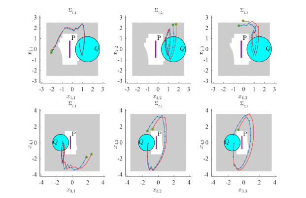
Figure 5: Simultaneous evolution of the state trajectories in the network of closed loop systems for $N=3$, with arbitrarily chosen initial states within the domain of the controllers. For each subplot, the gray region is the domain of the abstract controller, the purple rectangle ($P$) in the middle is the obstacle, and the cyan circle ($Q$) is the target of the reachability objective. The red and blue lines are the continuous and abstract trajectories respectively, which start from the green dots.

In this example, because of the similarity of the subsystems and their specifications, we only need to solve two synthesis problems; we synthesize two control functions $\hat{f}^{c}_{1}$ and $\hat{f}^{c}_{2}$ for $\mathcal{P}_{{\tau\eta_{i}\omega_{i}}}(\Sigma_{1,i})$ and $\mathcal{P}_{{\tau\eta_{i}\omega_{i}}}(\Sigma_{2,i})$ w.r.t. the specifications $\varphi_{{\tau\eta_{i}\omega_{i}},1,i}$ and $\varphi_{{\tau\eta_{i}\omega_{i}},2,i}$, respectively, for some $i\in[1,N]$. In this particular case, $\varphi_{{\tau\eta\omega},j,i}$ is the LTL specification in (36) over the $\varepsilon_{i}$-deflation of the target and save sets. Refining these abstract controllers as discussed in Sec. VII results in a network of closed loop systems whose simultaneously generated trajectories are depicted in Fig. 5. The simulation was stopped after each of the systems has fulfilled its reachability objective at least once. Fig. 5 shows that all local closed loops robustly and independently satisfy their objectives.

N=100

Now we increase the size of the system to $N=100$, with a total number of $400$ state variables. To our best knowledge, no existing tool for monolithic synthesis scales to such a large system. However, our method scales perfectly as controller synthesis only needs to be performed for systems with two state variables as discussed before. The resultant continuous trajectories of the network of closed loop systems are depicted in Fig. 6. For clarity of presentation every trajectory was stopped when it first met its reachability objective. It is observed that each of the subsystems fulfills it’s specification.

We want to point out that $N$ could have been increased to any arbitrarily large value without affecting the sound behavior of the local controllers for each subsystem. The reason is that the abstraction error of each subsystem in the network is immune to the abstraction error of non-neighboring subsystems. This is easy to verify from Inq. (21), where we use only the upper bounds (i.e. the most pessimistic bounds) on the abstraction errors of the neighbors in $\tilde{\varepsilon}_{i}$. Since the abstraction error of each subsystem does not depend on the non-neighboring subsystems, and moreover the number of neighbors of all but one subsystems in the network remain the same when we increase $N$, no matter what value $N$ might take soundness is guaranteed.

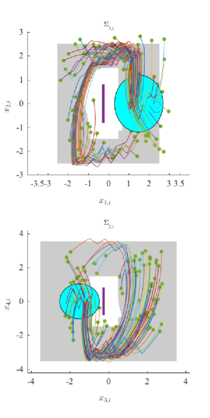
Figure 6: Simultaneous evolution of the systems for $N=100$ with arbitrary initial points within the domain of the controllers. For each subplot, the state space has the same representation same as in Fig. 5 (annotations are omitted). The lines represent the continuous trajectories of various systems which start from the green dots.

IX Conclusion

In this paper we introduced disturbance bisimulation as an equivalence relation between two metric systems having the same metric on their state spaces, and showed that disturbance bisimulation is closed under system composition. We extended disturbance bisimulation to two different abstractions of nonlinear dynamic systems by suitably abstracting the time, input-space and state-space. Finally we show how exploiting the closure under composition property, one can use disturbance bisimilar abstractions for decentralized controller synthesis with omega-regular control objectives. We demonstrate the effectiveness of our theory by an example.

References

• [1] P. Tabuada, Verification and control of hybrid systems: a symbolic approach.   Springer Science & Business Media, 2009.
• [2] A. Girard, “Approximately bisimilar finite abstractions of stable linear systems,” in HSCC’07, vol. 4416, pp. 231–244, 2007.
• [3] G. Pola, A. Girard, and P. Tabuada, “Approximately bisimilar symbolic models for nonlinear control systems,” Automatica, vol. 44, no. 10, pp. 2508–2516, 2008.
• [4] G. Pola and P. Tabuada, “Symbolic models for nonlinear control systems: Alternating approximate bisimulations,” SIAM Journal on Control and Optimization, vol. 48, no. 2, pp. 719–733, 2009.
• [5] M. Zamani, G. Pola, M. Mazo, and P. Tabuada, “Symbolic models for nonlinear control systems without stability assumptions,” IEEE Transactions on Automatic Control, vol. 57, no. 7, pp. 1804–1809, 2012.
• [6] E. A. Emerson and C. S. Jutla, “Tree automata, mu-calculus and determinacy,” in Proceedings of 32th Annual Symposium on Foundations of Computer Science, pp. 368–377, 1991.
• [7] O. Maler, A. Pnueli, and J. Sifakis, “On the synthesis of discrete controllers for timed systems,” in STACS’95, ser. LNCS.   Springer, 1995, vol. 900, pp. 229–242.
• [8] M. Mazo Jr., A. Davitian, and P. Tabuada, “PESSOA: A tool for embedded controller synthesis,” in CAV 2010, ser. Lecture Notes in Computer Science, vol. 6174.   Springer, 2010, pp. 566–569.
• [9] M. Rungger and M. Zamani, “SCOTS: A tool for the synthesis of symbolic controllers,” in HSCC’16.   ACM, 2016, pp. 99–104.
• [10] P. Nilsson, O. Hussien, A. Balkan, Y. Chen, A. D. Ames, J. W. Grizzle, N. Ozay, H. Peng, and P. Tabuada, “Correct-by-construction adaptive cruise control: Two approaches,” IEEE Trans. Contr. Sys. Techn., vol. 24, no. 4, pp. 1294–1307, 2016.
• [11] A. D. Ames, P. Tabuada, B. Schürmann, W. Ma, S. Kolathaya, M. Rungger, and J. W. Grizzle, “First steps toward formal controller synthesis for bipedal robots,” in HSCC’15.   ACM, 2015, pp. 209–218.
• [12] A. Borri, G. Pola, and M. D. D. Benedetto, “Symbolic models for nonlinear control systems affected by disturbances,” Int. J. Control, vol. 85, no. 10, pp. 1422–1432, 2012.
• [13] M. Zamani, P. M. Esfahani, R. Majumdar, A. Abate, and J. Lygeros, “Symbolic control of stochastic systems via approximately bisimilar finite abstractions,” IEEE Trans. Automat. Contr., vol. 59, no. 12, pp. 3135–3150, 2014.
• [14] M. Zamani, A. Abate, and A. Girard, “Symbolic models for stochastic switched systems: A discretization and a discretization-free approach,” Automatica, vol. 55, pp. 183–196, 2015.
• [15] M. Zamani, M. Rungger, and P. M. Esfahani, “Construction of approximations of stochastic control systems: A compositional approach,” in CDC’15.   IEEE, 2015, pp. 525–530.
• [16] G. C. Goodwin, S. F. Graebe, and M. E. Salgado, “Control system design,” Upper Saddle River, 2001.
• [17] Y. Tazaki and J.-i. Imura, “Bisimilar finite abstractions of interconnected systems,” HSCC’08, pp. 514–527, 2008.
• [18] M. Rungger and M. Zamani, “Compositional construction of approximate abstractions,” in Proceedings of the 18th International Conference on Hybrid Systems: Computation and Control.   ACM, 2015, pp. 68–77.
• [19] M. Zamani and M. Arcak, “Compositional abstraction for networks of control systems: A dissipativity approach,” arXiv preprint arXiv:1608.01590, 2016.
• [20] G. Pola, P. Pepe, and M. D. Benedetto, “Symbolic models for networks of discrete-time nonlinear control systems,” in American Control Conference, ACC 2014.   IEEE, 2014, pp. 1787–1792.
• [21] G. Pola, P. Pepe, and M. Di Benedetto, “Symbolic models for networks of control systems,” IEEE Transactions on Automatic Control, 2016, to appear.
• [22] E. Dallal and P. Tabuada, “On compositional symbolic controller synthesis inspired by small-gain theorems,” in CDC’15.   IEEE, 2015, pp. 6133–6138.
• [23] J. Liu and N. Ozay, “Abstraction, discretization, and robustness in temporal logic control of dynamical systems,” in HSCC ’14, 2014, pp. 293–302.
• [24] A. Girard, G. Gössler, and S. Mouelhi, “Safety controller synthesis for incrementally stable switched systems using multiscale symbolic models,” IEEE Transactions on Automatic Control, vol. 61, no. 6, pp. 1537–1549, 2016.
• [25] D. Angeli, “A lyapunov approach to incremental stability properties,” IEEE Transactions on Automatic Control, vol. 47, no. 3, pp. 410–421, 2002.
• [26] A. Girard, G. Pola, and P. Tabuada, “Approximately bisimilar symbolic models for incrementally stable switched systems,” IEEE Transactions on Automatic Control, vol. 55, no. 1, pp. 116–126, 2010.
• [27] H. K. Khalil, Nonlinear Systems.   Prentice-Hall, New Jersey, 1996.
• [28] S. Dashkovskiy, H. Ito, and F. Wirth, “On a small gain theorem for iss networks in dissipative lyapunov form,” European Journal of Control, vol. 17, no. 4, pp. 357–365, 2011.
• [29] A. Girard, “A composition theorem for bisimulation functions,” arXiv preprint arXiv:1304.5153, 2013.
• [30] “Controller synthesis for safety and reachability via approximate bisimulation,” Automatica, vol. 48, no. 5, pp. 947 – 953, 2012.
• [31] “Synthesis of reactive(1) designs,” Journal of Computer and System Sciences, vol. 78, no. 3, pp. 911 – 938, 2012.
• [32] G. Reissig, A. Weber, and M. Rungger, “Feedback refinement relations for the synthesis of symbolic controllers,” IEEE Transactions on Automatic Control, vol. 62, no. 4, pp. 1781–1796, 2017.