Lectures on
Higher-Gauge Symmetries from Nambu Brackets
and
Covariantized M(atrix) Theory

Abstract

This lecture consists of three parts. In part I, an overview is given on the so-called Matrix theory in the light-front gauge as a proposal for a concrete and non-perturbative formulation of M-theory. I emphasize motivations towards its covariant formulation. Then, in part II, I turn the subject to the so-called Nambu bracket and Nambu mechanics, which were proposed by Nambu in 1973 as a possible extension of the ordinary Hamiltonian mechanics. After reviewing briefly Nambu’s original work, it will be explained why his idea may be useful in exploring higher symmetries which would be required for covariant formulations of Matrix theory. Then, using this opportunity, some comments on the nature of Nambu mechanics and its quantization are given incidentally: though they are not particularly relevant for our specialized purpose of constructing covariant Matrix theory, they may be of some interests for further developments in view of possible other applications of Nambu mechanics. The details will be relegated to forthcoming publications. In part III, I give an expository account of the basic ideas and main results from my recent attempt to construct a covariantized Matrix theory on the basis of a simple matrix version of Nambu bracket equipped with some auxiliary variables, which characterize the scale of M-theory and simultaneously play a crucial role in realizing (dynamical) supersymmetry in a covariant fashion.

Part I : An Overview on Matrix Theory

1 The M-theory conjecture

M-theory was conjectured in the mid 90s as a hidden theory: it would play a crucial pivotal role in a possible non-perturbative formulation unifying five perturbative string theories which had been established in the mid 80s. The basic tenets of M-theory are as follows:

1. It achieaves a complete unification of strings and D-branes in a compactified $(10,1)$ dimensional spacetimes.

2. There is a unique fundamental length scale $\ell_{11}$ corresponding to the 11 dimensional Planck scale. Together with the radius $R_{11}$ of compactification of (10,1)-dimensional spacetime to $(9,1)$ dimensional spacetimes corresponding to type IIA string theory (and $E_{8}\times E_{8}$ heterotic string theory), it sets the string scale $\ell_{s}$ and string coupling constant $g_{s}^{(A)}$ as

   $$\ell_{s}^{2}=\ell_{11}^{3}R_{11}^{-1},\qquad g_{s}^{(A)}=(R_{11}\ell_{11}^{-1})^{3/2}=R_{11}/\ell_{s}.$$

   The scales and couplings of the other perturbative string theories are related by duality relations. For instance, the so-called S-duality of type IIB theory is explained by introducing additional compactification along one of remaining spatial directions with radius $R_{10}$: The type IIA and IIB theories are then related by a T-duality transformation,

   $$R_{10}\rightarrow\ell_{s}^{2}/R_{10},\quad g_{s}^{(A)}\rightarrow g_{s}^{(B)}=g_{s}^{(A)}\ell_{s}/R_{10}=R_{11}/R_{10}.$$

   Thus the S-duality transformation $g_{s}^{(B)}\rightarrow 1/g_{s}^{(B)}$ of type IIB theory corresponds simply to the interchange of 10th and 11th directions, $(R_{10},R_{11})\leftrightarrow(R_{11},R_{10})$.

3. The underlying dynamical degrees of freedom are super-membranes (or M2-banes) which have an “electrical charge” coupled to a 3-form gauge field as particular components of physical degrees of freedom of super-membranes. There are also excitations, called M5-branes, which correspond to excitations which are electro-magnetically dual to super-membranes. After compactification to $(9,1)$ dimensions, the super-membranes behave either as fundamental strings when one of their two spatial directions is wrapped along the compactified direction, or as D2-branes when none of the spatial directions of supermembranes are wrapped along the compactified direction.

In particular, as a consequence of these assumptions, gravitons in compactified 11 dimensions, if momentum along the compactified direction is zero, are the ground-state modes of strings at least in the limit of small compactifcation radius, and if they have non-zero momentum along the compactified direction, are the Kaluza-Klein modes which should coincide with the ground-state of wrapped super-membrane with non-zero momentum in the same direction and are identified with D0-branes (or D-particles) of type IIA string theory. This picture is valid for small compactification radius $R_{11}\ll\ell_{11}$ with fixed $\ell_{s}=\ell_{11}/(R_{11}/\ell_{11})^{1/2}=\ell_{11}g_{s}^{-1/3}$. The latter relation shows that, in the opposite limit of de-compactification $R_{11}\gg\ell_{11}$ with fixed $\ell_{11}$, we have $\ell_{s}\rightarrow 0$ and $g_{s}^{(A)}\rightarrow\infty$, namely, a very singular limit of type IIA string theory corresponding to infinite string tension and infinite string coupling. Since string theory has been known only perturbatively in the limit of infinitely small $g_{s}$, it is very difficult to imagine how such a peculiar limit should be formulated. One suggestive expectation is that M-theory might be described by some degrees of freedom corresponding to short strings and its KK modes or D0-branes but with some intrinsic non-perturbative interactions among them, which would make possible some mechanisms generating not only supermembranes, but also other physical degrees of freedom as some sort of bound states of D0-branes (and short strings).

2 The dynamics of (Super)membranes

A similar picture which seems to be compatible with the foregoing viewpoint naturally emerges itself if we envisage the dynamics of super-membranes. To study the relativistic dynamics of membranes assuming flat 11-dimensional spacetimes, we can start from a typical action

$$A=-\frac{1}{\ell_{11}^{3}}\int d^{3}\xi\Bigl{(}\frac{1}{e}\{X^{\mu},X^{\nu},X^{\sigma}\}\{X_{\mu},X_{\nu},X_{\sigma}\}-e\Bigr{)}+\ldots$$ (1)

where $X^{\mu}(\xi)$ ($\mu,\nu,\dots,\in(1,2,\ldots,10,0)$) are the target space coordinates of the membrane and the ellipsis ($\ldots$) means other contributions involving in particular the fermionic degrees of freedom. Throughout this lecture, we always use Einstein’s summation convention for spacetime (and/or space) indices in target space. The variable $e=e(\xi)$ is an auxiliary field, transforming as a world-volume density under 3-dimensional diffeomorphism with respect to the parameterization $(\xi^{1},\xi^{2},\xi^{0})=(\sigma_{1},\sigma_{2},\tau)$ of the world-volume of a membrane. We also used the following notation,

$$\{X^{\mu},X^{\nu},X^{\sigma}\}\equiv\sum_{a,b,c\in(1,2,0)}\epsilon^{abc}\partial_{a}X^{\mu}\partial_{b}X^{\nu}\partial_{c}X^{\sigma},$$ (2)

which will be called “Nambu-bracket” (or Nambu-Poisson bracket). The standard form (Dirac-Nambu-Goto type) of the world-volume action is obtained by eliminating the auxiliary field $e$.

Unfortunately, this is a notoriously difficult system to deal with, especially with respect to quantization. Only tractable way which allow us a reasonably concrete treatment so far is to adopt the light-front gauge $X^{+}\equiv X^{10}+X^{0}=\tau$, breaking 11-dimensional Lorentz covariance.[1] After a further (still partial) gauge-fixing of the residual (time-dependent) re-parametrizations of spatial coordinates $(\sigma_{1},\sigma_{2})$ by demanding that the induced metric of the world-volume takes an orthogonal form $ds^{2}=g_{00}d\tau^{2}+g_{rs}d\sigma^{r}d\sigma^{s}$ ($r,s\in(1,2)$) with $g_{rs}=\partial_{r}X^{i}\partial_{s}X^{i}$ and also that light-like momentum density is a constant $P^{+}=P^{10}+P^{0}$ with the normalization $\int d^{2}\sigma=1$, we are left with a constraint

$$\{P_{i},X^{i}\}+\cdots\approx 0,$$

where

$$\{A,B\}\equiv\partial_{1}A\partial_{2}B-\partial_{2}A\partial_{1}B$$

for arbitrary pair of functions $A,B$, and the effective Hamiltonian, in the unit $\ell_{11}=1$ for notational brevity :

$$H=\int d^{2}\sigma\frac{1}{P^{+}}(P_{i}^{2}+\frac{1}{2}\{X^{i},X^{j}\}^{2})+\cdots.$$

where the indices $i,j,\ldots,$ of the target-space coordinates $X^{i}$ run over only SO(9) transverse directions $(1,2,\ldots,9)$. The above constraint demands that the system is invariant under infinitesimal (time-independent) area-preserving diffeomorphism of spatial coordinates which still remains as residual gauge symmetry after all of the above gauge-fixing conditions:

$$\delta_{F}X^{i}=(\partial_{1}F\partial_{2}-\partial_{2}F\partial_{1})X^{i}=\{F,X^{i}\}$$ (3)

with $F=F(\sigma)$ is an arbitrary function of the spatial world-volume coordinates.

As a 3-dimensional field theory, this is still a very nontrivial system without standard kinetic-potential terms, such as $(\partial_{1}X^{i})^{2}+(\partial_{2}X^{i})^{2}$, of second order, but being instead equipped with (non-renormalizable) quartic interaction terms with four derivatives. A useful suggestion for controlling this system was made by Goldstone and Hoppe [2] in the early 80s (and developed further in ref. [3] later). Namely, we can regularize this system by replacing the fields $X^{i}(\xi)$ by finite $N\times N$ hermitian matrices $X^{i}_{ab}$ where the matrix indices $a,b,\ldots$ now run from 1 to $N$. Then, the above Hamiltonian is replaced by

$$H=\frac{1}{P^{+}}{\rm Tr}\Bigl{(}\boldsymbol{P}_{i}^{2}-\frac{1}{2}[\boldsymbol{X}^{i},\boldsymbol{X}^{j}]^{2}\Bigr{)}+\cdots,$$ (4)

where and in what follows we use slanted boldface symbols $\boldsymbol{X}^{i},\boldsymbol{P}^{i}$ (hence, $(\boldsymbol{X}^{i})_{ab}\equiv X^{i}_{ab}$) for matrices when the matrix indices $(a,b,\ldots)$ are supressed. $\boldsymbol{P}_{i}$’s are of course canonical-momentum matrices corresponding to the canonical-coordinate matrices $\boldsymbol{X}^{i}$’s. The constraint corresponding to area-preserving diffeomorphism is now replaced by

$$[\boldsymbol{P}_{i},\boldsymbol{X}^{i}]+\cdots\approx 0,$$ (5)

which generates infinitesimal unitary (SU($N$)) transformations of matrix variables:

$$\delta_{F}\boldsymbol{X}^{i}=i[\boldsymbol{F},\boldsymbol{X}^{i}],\quad\delta_{F}\boldsymbol{P}_{i}=i[\boldsymbol{F},\boldsymbol{P}_{i}]$$

where $\boldsymbol{F}$ is an arbitrary (time-independent) hermitian matrix.

It should be clear that the matrix regularization is based on a formal but natural analogy between classical brackets $\{\,\,,\,\,\}$ and commutator $i[\,\,,\,\,]$. The basic idea here is that given a finite world-volume with fixed topology we can alway use some appropriate Fourier-like representation for the fields $X^{i}(\sigma),P_{i}(\sigma)$ and take the resulting discretized Fourier components of them as dynamical variables. If we have an appropriate way of truncating the infinite number of such Fourier components into a finite set of components by keeping the remnant of the area-preserving diffeormorphism group as a symmetry group of this finite set, it would provide a desirble regularized version of the original system. It is not unreasonable to expect that, for sufficiently large $N$, the above system would be capable of approximating arbitrary kinds of fixed topology of supermembrane in some classical limit and, in quantum theory, of describing the dynamics of supermembranes and other physical objects. Now with a finite number of degrees of freedom, the system is completely well defined and therefore amenable to any non-perturbative studies including computer simulations. Matrix models of this kind would play, at the very least, the role of the same sort that lattice gauge theories are playing in non-perturbative studies of gauge field theories. The importance of such tractable system in this sense should not be underestimated in view of the genuine dynamical nature of the M-theory conjecture.

3 M(atrix) theory proposal in the DLCQ scheme

One of various remarkable facts concerning the matrix regularization of supermembrane is that the same system appears as the low-energy effective theory[5] of $N$ D0-branes. In the same unit $\ell_{11}=1$ ($\ell_{s}=g_{s}^{-1/3},R_{11}=\ell_{s}^{-2}=g_{s}^{2/3}$) as above, the Hamiltonian is

$$H_{{\rm D0}}=\frac{1}{2}g_{s}^{2/3}{\rm Tr}\Bigl{(}\boldsymbol{P}_{i}^{2}-\frac{1}{2}[\boldsymbol{X}_{i},\boldsymbol{X}_{j}]^{2}\Bigr{)}+\cdots,$$ (6)

where the momentum is given as

$$\boldsymbol{P}_{i}=\partial_{0}\boldsymbol{X}_{i}+i[\boldsymbol{A},\boldsymbol{X}^{i}]$$

with $\boldsymbol{A}$ being an SU($N$) gauge matrix-field corresponding to local gauge transformation

$$\delta\boldsymbol{X}_{i}=i[\boldsymbol{F},\boldsymbol{X}_{i}],$$ (7)

$$\delta\boldsymbol{A}=i[\boldsymbol{F},\boldsymbol{A}]-\frac{d\boldsymbol{F}}{dt}.$$ (8)

In this case, the constraint (5) appears as the Gauss constraint corresponding to this local gauge symmetry. Thus the original diffeomorphism symmetry is now interpreted as a local gauge symmetry. It should be noted that the gauge field $\boldsymbol{A}$ does not play any dynamical role other than giving the Gauss constraint, since the present system is only (0,1)-dimensional as a gauge field theory.

The diagonal components $(X_{i\,aa},P_{i\,aa})$ of the matrices are interpreted to represent the motion of D0-branes, whereas the off-diagonal components are supposed to correspond to the lowest dynamical degrees of freedom of open strings connecting them. Thus the zero-mode kinetic energy of D0-branes is $\frac{1}{2}g_{s}^{2/3}\sum_{a=1}^{N}(P_{i\,aa})^{2}$. This coincides with (4) if we assume $P^{+}=2g_{s}^{-2/3}=2R_{11}^{-1}$. The latter identification is consistent with the assumption that D0-brane is a Kaluza-Klein mode with a unit quantized momentum along the compactified circle of radius $R_{11}$: if $R_{11}$ is sufficiently small, then we have

$$P_{10}=R_{11}^{-1},\quad P^{0}=\sqrt{P_{i}^{2}+P_{10}^{2}}\rightarrow R_{11}^{-1},$$

and hence $P^{+}\rightarrow 2R_{11}^{-1}$ for each independent D0-brane. This is the limit where we can trust the above effective low-energy Hamiltonian for D0-branes (of mass $1/R_{11}$) in weak-coupling string theory in un-compactified $(9,1)$ dimensions. Note that if we separate out the center-of-mass momentum $P_{\circ}^{i}$ and the traceless part of the matrices

$$P_{\circ}^{i}\equiv{\rm Tr}\boldsymbol{P}^{i},$$

we can write

$$H=\frac{1}{2P_{\circ}^{10}}(P_{\circ i}^{2}+\hat{H}),\quad P_{\circ}^{10}=NR_{11}^{-1},$$

$$\hat{H}=N{\rm Tr}\Bigl{(}\hat{\boldsymbol{P}}_{i}^{2}-\frac{1}{2}[\boldsymbol{X}^{i},\boldsymbol{X}^{j}]\Bigr{)}+\cdots,$$ (9)

where and in what follows we denote the traceless part of the matrices by putting $\,\hat{}\,$ symbol: $\hat{\boldsymbol{P}}_{i}=\boldsymbol{P}_{i}-\frac{1}{N}P_{\circ i}$. $\hat{H}$ involves only the traceless part of the matrix variables.

Now what should be the interpretation of the above coincidence? Suppose that we consider an ordinary relativistic system of $N$ interacting particles in flat spacetime. If we extract the center-of-mass momentum $P^{\mu}_{\circ}$, the system would have invariably a mass-shell constraint of the form

$$P^{\mu}_{\circ}P_{\circ\mu}+M_{{\rm eff}}^{2}=0,$$ (10)

where $M^{2}_{{\rm eff}}$ is the effective squared mass which describes internal (Lorentz-invariant) dynamics of the whole system. Using the light-like components, this can be expressed as

$$-P_{\circ}^{-}\equiv P_{\circ}^{0}-P_{\circ}^{10}=\sqrt{P_{\circ i}^{2}+(P_{\circ}^{10})^{2}+M_{{\rm eff}}^{2}}-P_{\circ}^{10}\rightarrow\frac{P_{\circ i}^{2}+M_{{\rm eff}}^{2}}{2P_{\circ}^{10}}$$ (11)

in the limit of large $P_{10}$, which corresponds to the so-called infinite momentum frame (IMF). Alternatively, we can use an exact relation using light-like components, irrespectively of $P_{10}$ being large or small,

$$-P^{-}_{\circ}=\frac{P_{\circ i}^{2}+M_{{\rm eff}}^{2}}{P^{+}_{\circ}},$$ (12)

which of course reduces to (11) in the limit $P_{\circ}^{10}\rightarrow\infty$. In the case of (12), we can assume further that the compactification is made directly along the light-like direction $X^{-}$ with radius $R$ corresponding to the quantization condition

$$P_{\circ}^{+}=2N/R,$$

by which (12) coincides with (9) if we identify $\hat{H}$ with $M^{2}_{{\rm eff}}$. This special compactification scheme along $X^{-}$ is known as the discrete light-cone quantization (DLCQ) in field theories. But we are now adopting this scheme to relativistic system of $N$ particles in configuration-space formulation, instead of relativistic local field theory where some subtleties are known with respect to its significance in non-perturbative properties of field theories.

A crucial difference of this interpretation from the IMF is that we can freely change the value of $R$ from infinitely small to infinitely large, by merely changing the Lorentz frame with any fixed $N$. In the IMF interpretation, on the contrary, the radius $R_{11}$ of compactification is fixed irrespectively of which Lorentz frame we are studying the system: thus for large $P^{10}_{\circ}=N/R_{11}$ we have to take large $N$ by assuming that each D-particle has fixed eleven-th momentum $1/R_{11}$.

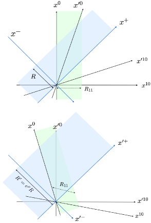
Figure 1: DLCQ: By a boost transformation along the compactified direction $x^{-}$ the radius of compactification can be continuously changed. Compare the upper and lower Minkowski diagrams showing expansion of $R$ to $R^{\prime}$.

Actually, it is not at all obvious whether such an interacting theory of particles in configuration-space formulation assumed in this argument is completely consistent, as it stands, with Lorentz invariance and principles of unitary quantum theory, within the restriction of a fixed number of particles without anti-particles. The peculiarity of the system such as (6) is that the particles are interacting in a manifestly non-local fashion through mediating open strings, which correspond to off-diagonal matrix elements and mix them with particle coordinates through local gauge transformations. We can think of such mixing as an extension of quantum statistics of ordinary particles to D-branes. This is an entirely novel situation that we have never encountered previously, before the advent of string theory and D-brane excitations. It is not evident whether (or to what extent) our experiences with relativistic local field theory are applicable to this system. Unfortunately, we have not acquired much improvement on true conceptual understandings on such non-locality and extended quantum statistics even after the two decades of various studies.

A very bold hypothesis made in [7][8][9], following the so-called BFSS conjecture [10] made prior to it, is that the above SU($N$) gauge theory is already an exact theory of 11-dimensional M-theory in the special DLCQ quantization scheme with finite $N$. Of course, in order to exhibit full 11-dimensional content of this theory under this assumption, we should be able to treat continuous values of $P_{\circ}^{+}$ in any fixed Lorentz frame. Thus definitely we have to take the limit $N\rightarrow\infty$ and $R\rightarrow\infty$ in the end. However, it is quite remarkable that even a finite-$N$ theory may have a definite and certain exact meaning related somehow to exact non-perturbative formulation of M-theory. It seems a pity that in spite of intensive studies made from the late 90s to the early 2000s, progress has practically stopped in the last decade. In this lecture, I would like to revisit and pursue the conjecture of the DLCQ Matrix theory as a working hypothesis in its strongest form.

For the validity of this hypothesis, there is a presumption that $\hat{H}$ is physically equivalent with the Lorentz-invariant mass-square $M^{2}_{{\rm eff}}$ for finite $N$. This must be true for arbitrary Lorentz transformations, which are not restricted to boosts along the compactified (10th) direction. Under general Lorentz transformation, the values of $P_{\circ}^{\pm}$ are mixed with transverse components $P_{\circ}^{i}$ of momenta. Therefore they must be continuously varying even with finitely fixed $N$. Here it is important to recall again that within the framework of the DLCQ scheme, the radius $R$ and hence $P_{\circ}^{+}$ are in fact regarded as continuously varying physical variables, since by boost transformations $x^{+}=x^{10}+x^{0}\rightarrow x^{\prime+}=x^{\prime 10}+x^{\prime 0}=e^{-\rho}x^{+},x^{-}=x^{10}-x^{0}\rightarrow x^{\prime-}=x^{\prime 10}-x^{\prime 0}=e^{\rho}x^{\prime-}$ along the $10$-th spatial direction we have transformations

$$P_{\circ}^{\pm}\rightarrow P^{\prime\pm}_{\circ}=e^{\mp\rho}P_{\circ}^{\pm}$$

or $R^{\prime}=e^{\rho}R$ with arbitrary value of $\rho$ (see Fig. 1).

Now the final goal of this lecture is to demonstrate how it is indeed possible to formulate a fully Lorentz-covariant Matrix theory such that $\hat{H}$ is physically equivalent to a Lorentz invariant mass-square $M_{{\rm eff}}^{2}$ representing the internal dynamics of the system. This will be achieved by realizing a higher gauge symmetry which extends the usual SU($N$) gauge symmetry, (7) and (8), such that after imposing appropriate light-like gauge conditions for the higher-gauge degrees of freedom, a manifestly Lorentz covariant formulation which we are going to propose here reduces to the light-front Matrix theory in the physical space of allowed states.

4 Clues toward higher-gauge symmetries

It is obvious that, to realize such a covariant system, we need a new kind of symmetries which encompass and extend the SU($N$) gauge symmetry of the light-front formulation. In particular, it is crucial for the DLCQ scheme that such higher symmetries are operational even for finite $N$. In that sense, the viewpoint that the matrix theory is just a mere regularization of supermembranes should be abandoned. In fact, the simple matrix theory explained in the previous section exhibits several notable features that indeed this theory itself has some fundamental significance, independently of its relation to supermembranes. It is to be noted, at the basis for such features, that the system can be regarded as a self-consisting universal system. This may be signified in the following serial patterns of the theories with increasingly larger gauge groups:

$\cdots\subset$ SU($N$) $\subset$ SU($N+1$)$\subset$ $\cdots\subset$ SU($N+M$) $\subset\cdots$,

and

$\cdots\subset$ SU($N_{1}$) $\subset$ SU($N_{1}$)$\times$ SU($N_{2}$)

$\subset$ SU($N_{1}+N_{2}$) $\subset$ SU($N_{1}+N_{2}$) $\times$ SU($N_{3}$) $\subset$ SU($N_{1}+N_{2}+N_{3}$) $\subset\cdots$,

and so on.

In other words, the system can in principle describe arbitrary multi-body states of physical objects which are represented by smaller sub-systems with hermitian sub-matrices. In this way, we can represent various many-body D-brane configurations and simulate their general-relativistic interactions, as reviewed in [11]. For example, it has been confirmed that 3-body nonlinear interactions of gravitons described by the classical Einstein action of 11 dimensional supergrvatity emerge correctly[12] even with finite $N$ through the perturbative loop effects of off-diagonal matrix elements. This evidences our view that the SU($N$) matrix theory of finite $N$ already has some fundamental meaning beyond a possible approximate regularized formulation of supermembranes.

With this caveat in mind, we can still extract some useful hints about desirable higher symmetries from the membrane analogy at least at a formal level. The SU($N$) gauge symmetry of light-front matrix theory corresponds mathematically to the area-preserving diffeomorphism (3) on the membrane side. The area-preserving diffeomorphism can be regarded as a gauge-fixed version of a more general volume-preserving diffeomorphism represented by

$$\delta X^{\mu}=\{F_{1},F_{2},X^{\mu}\},$$ (13)

which is the residual symmetry of the classical action (1) after we adopt the condition $e=1$, partially fixing the general 3-dimensional diffeomorphism. One arbitrary function $F$ of the area-preserving transformation which corresponds to one arbitrary hermitian matrix $\boldsymbol{F}$ is now extended to two arbitrary functions $F_{1}$ and $F_{2}$ in (13).

We call the infinitesimal transformation (13) the Nambu transformation, since Nambu originated a generalization[13] of Hamiltonian dynamics by proposing dynamical systems in 3-dimensional “phase space” $(\xi_{1},\xi_{2},\xi_{3})$ in which the equations of motion are

$$\frac{d\xi_{a}}{dt}=\{H,G,\xi_{a}\}\equiv L\xi_{a},$$ (14)

$$L=\sum_{a}L_{a}\frac{\partial}{\partial\xi_{a}},\quad L_{a}=\sum_{b,c}\frac{1}{2}\epsilon_{abc}\frac{\partial(H,G)}{\partial(\xi_{b},\xi_{c})}$$ (15)

with two Hamitonian-like generators $H=H(\xi)$ and $G=G(\xi)$. In seeking for higher-gauge symmetries, it seems natural to try first to construct some matrix version of the Nambu transformation, in analogy with the fact that the usual SU($N$) transformation is the matrix version of (3). As a preparation for proceeding to such a task, I will give a brief review on some salient features of Nambu mechanics focusing its symmetry structure in the next part.

Part II : Nambu’s Generalized Hamitonian Mechanics

5 A brief review of Nambu mechanics

As a motivation for his proposal of a generalized Hamiltonian dynamics, Nambu stressed that the Liouville theorem for the Hamitonian equations of motion is naturally extended to (14) as

$$\sum_{a}\partial_{a}L_{a}=0,$$ (16)

expressing volume-perserving nature of general transformation (13). His motivation was a possible generalization of statistical mechanics such that the canonical ensemble is specified by two or more “temperatures” corresponding to the existence of many conserved Hamiltonians.

The usual canonical Poisson bracket is now replaced by a canonical “Nambu bracket” which has a triplet structure:

$$\{\xi_{a},\xi_{b},\xi_{c}\}=1\,\,\mbox{iff $(a,b,c)$ is a cyclical permutation of $(1,2,3)$}.$$ (17)

A notable example from well-known dynamical systems which realizes this structure is the Euler equations of motion of a rigid top: if we regard the 3 components $(\mu_{1},\mu_{2},\mu_{3})$ of angular momentum in the body-fixed frame as canonical coordinates $\xi_{a}=\mu_{a}$,

$$\frac{d\mu_{a}}{dt}=-\sum_{b,c}\epsilon_{abc}\Bigl{(}\frac{1}{I_{b}}-\frac{1}{I_{c}}\Bigr{)}\mu_{b}\mu_{c}=\{H,G,\mu_{a}\}$$ (18)

where

$$H=\sum_{a}\frac{\mu_{a}^{2}}{2},\quad G=\sum_{a}\frac{\mu_{a}^{2}}{2I_{a}}$$

with $I_{a}$’s being the principal momenta of inertia of an assymmetrical top.

Nambu noted that the system of equations (14) have a “gauge” symmetry with respect to transformation $(H,G)\rightarrow(H^{\prime},G^{\prime})$ of the pair of Hamiltonians defined by $\frac{\partial(H^{\prime},G^{\prime})}{\partial(H,G)}=1$ which can be expressed equivalently as

$$H\delta G-H^{\prime}\delta G^{\prime}=\delta f\quad or\quad\frac{\partial f}{\partial G}=H,\,\,\frac{\partial f}{\partial G^{\prime}}=-H^{\prime},$$ (19)

where $f=f(G,G^{\prime})$ is an arbitrary function of $G$ and $G^{\prime}$ as a generating function which implicitly determines the transformation. He also correctly noted that this is not the most general gauge transformation from the viewpoint of general volume-preserving transformations. In the latter viewpoint, (19) would be slightly generalized to the transformations of the following form:

$$H\frac{\partial G}{\partial\xi_{a}}-H^{\prime}\frac{\partial G^{\prime}}{\partial\xi_{a}}=\frac{\partial S}{\partial\xi_{a}},$$ (20)

with an arbitrary function $S=S(\xi_{a})$ of $\xi_{a}$’s, instead of the form $f(G(\xi),G^{\prime}(\xi))$. The reason for Nambu’s remark is originated from the fact that $L_{a}$ defined in (15) is not the most general form satisfying (16), even if we consider arbitrary pair $(H,G)$. Locally, the most general form of the vector $L_{a}$ is

$$L_{a}=\frac{1}{2}\sum_{b,c}\epsilon^{abc}(\partial_{b}A_{c}-\partial_{c}A_{a})$$ (21)

with some vector gauge field $A_{a}(\xi)$, in terms of which the general gauge transformation keeping $L_{a}$ invariant is

$$\delta A_{a}=\partial_{a}S.$$ (22)

This would lead to (20). The form (15) corresponds to a special form

$$A_{a}=H\partial_{a}G.$$

However, the form (22) is not ensured in general by (19) for an arbitrary scalar function $S(\xi)$. The situation is in contrast to ordinary Hamilton mechanics where the vector field $L_{a}=\sum_{b}\epsilon^{ab}\partial_{b}F$ with an arbitrary scalar field $F$ locally exhausts the area-preserving condition $\partial_{a}L_{a}=0$. Nambu suggested that, to exhaust the most general form satisfying the latter condition in terms of triple bracket, the equations of motion may be extended to

$$\frac{d\xi_{\ell}}{dt}=\sum_{i}\{H_{i},G_{i},\xi_{\ell}\},\quad or\quad A_{a}=\sum_{i}H_{i}\partial_{a}G_{i}$$ (23)

by introducing multiple pairs $(H_{i},G_{i})$ instead of a single pair $(H,G)$. Then in general there is no manifestly conserved “Hamiltonians”, somewhat contrary to Nambu’s original motivation for extending statistical mechanics. With this generalization, the above gauge transformation must be generalized to

$$\sum_{i}(H_{i}\delta G_{i}-H^{\prime}_{i}\delta G^{\prime}_{i})=\delta f,\quad\frac{\partial f}{\partial G_{i}}=H_{i},\,\,\frac{\partial f}{\partial G^{\prime}_{i}}=-H^{\prime}_{i}.$$

which then allows one to set

$$\sum_{i}\Bigl{(}H_{i}\frac{\partial G_{i}}{\partial\xi_{a}}-H^{\prime}\frac{\partial G^{\prime}_{i}}{\partial\xi_{a}}\Bigr{)}=\frac{\partial S}{\partial\xi_{a}}$$

for an arbitrary function $S(\xi)$.

If we had started from the general form (21) for the equations of motion from the beginning, a motivation for introducing the triple bracket and canonical structure such as (17) would not arise, since then the role of Hamiltonians would have been played directly by the vector gauge fields $A_{a}$: no need to introduce pairs $(H_{i},G_{i})$. In that sense, it was fortunate for us that Nambu insisted on generalizing Hamilton mechanics in his way using the triple bracket.

Nambu further studied canonical transformations $\xi_{a}\rightarrow\xi^{\prime}_{a}$ of canonical coordinates which preserve (17). Restricting to the simplest case of linear transformations, he noticed disappointedly that there is a difficulty in extending the canonical structure to higher-dimensional phase space, $\{(\xi^{(p)}_{1},\xi_{2}^{(p)},\xi_{3}^{(p)});p=1,\ldots,n\}$, of $3n$-dimensions, on the basis of a naturally looking postulate that the canonical bracket obeys

$$\{\xi_{\ell}^{(p)},\xi_{m}^{(q)},\xi_{n}^{(r)}\}\equiv 1\,\, \mbox{iff }(\ell,m,n)\in\mbox{cyclic permutations of }(1,2,3)$$

$$\mbox{ and }p=q=r,$$ (24)

in a naive analogy with the Hamilton mechanics. The problem is that the equations (14) cannot preserve this canonical structure whenever the time development mixes different triplets with different $p$’s. This implies that from the viewpoint of canonical structure it is not possible to extend the Nambu mechanics to coupled many-body systems, in spite of several subsequent attempts toward such directions.

On the other hand, it is easy to generalize this system to an $N$-dimensional phase space $(\xi_{1},\ldots,\xi_{N})$ such that the time evolution is described by a set of $N-1$ Hamitonians $(H_{1},H_{2},\ldots,H_{N-1})$ :

$$\frac{d\xi_{a}}{dt}=\{H_{1},H_{2},\ldots,H_{N-1},\xi_{a}\}\equiv\frac{\partial(H_{1},\ldots,H_{N-1},\xi_{a})}{\partial(\xi_{1},\ldots,\xi_{N-1},\xi_{N})}.$$

Obviously, this preserves the $N$-dimensional volume as a straightforward extension of the case $N=3$. With respect to symmetries, these extended systems inherit the same problems as in $N=3$ with respect to possible extensions to $nN$-dimensional phase space. In the present lecture, we restrict ourselves only to the case $N=3$ and $n=1$.

One of Nambu’s further concerns was to examine whether or not the above structure could be extended to quantum theory. For that purpose, he considered the problem how the triple bracket defined by Jacobian determinant in classical theory can be mapped to some algebraic structure denoted by $[A,B,C]$, which is required to preserve the basic properties of the classical bracket, namely,

1. skew symmetry:

   $$[A,B,C]=-[B,A,C]=[B,C,A]=\cdots,$$ (25)

2. derivation law:

   $$[A_{1}A_{2},B,C]=[A_{1},B,C]A_{2}+A_{1}[A_{2},B,C],\quad{\rm etc}.$$ (26)

In particular, he postulates the following triple commutator as a candidate for quantum triple bracket:

$$[A,B,C]_{{\rm N}} \equiv ABC+BCA+CAB-BAC-ACB-CBA$$

$$=A[B,C]+B[C,A]+C[A,B],$$ (27)

and correspondingly the generalized Heisenberg equations of motion,

$$i\frac{dF}{dt}=[H,G,F]_{{\rm N}}.$$

In this definition, only the property (a) is manifestly satisfied, but not (b) automatically. So he discussed various possibilities of algebraic structures for the set of operators $H,G,\ldots,F,\ldots$, including possible generalizations as (23), by studying slightly weakened versions of these conditions. Unfortunately, however, the main conclusion was that it was difficult to realize quantization nontrivially. Nambu then studied the possibilities of using non-associative algebras, but his conclusion was again not definitive.

6 The fundamental identity and canonical structure

Further developments of Nambu mechanics rested largely upon a seminal work by Takhtajan[14] which appeared after two decades since Nambu’s original proposal. In this work, it was pointed out that there exists an important identity (now known as the “Fundamental Identity”, FI) satisfied by the Nambu bracket, which generalizes the Jacobi identity in the case of Poisson bracket. For an arbitrary set of five functions $(F_{1},\ldots,F_{5})$, it takes the form

$$\{F_{1},F_{2},\{F_{3},F_{4},F_{5}\}\}=\{\{F_{1},F_{2},F_{3}\},F_{4},F_{5}\}$$

$$+\{F_{3},\{F_{1},F_{2},F_{4}\},F_{5}\}+\{F_{3},F_{4},\{F_{1},F_{2},F_{5}\}\}.$$ (28)

This ensures that the canonical structure (17) is preserved by the time evolution described by (14), as can be seen by applying this identity with $F_{1}=H,F_{2}=G$ and $F_{3}=\xi_{1},F_{4}=\xi_{2},F_{5}=\xi_{3}$. The same can be said for general infinitesimal canonical transformation defined by

$$\delta\xi_{a}=\{F_{1},F_{2},\xi_{a}\}$$ (29)

with a pair $(F_{1},F_{2})$ of arbitrary functions of the canonical coordinates. This clarifies the reason why it is difficult to generalize the system to interacting many-body cases. For instance, the postulate (24) does not in fact satisfy the FI. This is in marked contrast to ordinary Hamiltonian mechanics. Also, the triple commutator (27) does not in general satisfy the FI. This partially explains the difficulties encountered in quantization.

These features indicate that the Nambu mechanics is a quite restricted dynamical system which is characterized by the stringent structure of the FI. In other words, we cannot expect the same kind of universality for Nambu mechanics as we have in the framework of Hamilton mechanics.

Nevertheless, we may also take a viewpoint, which is complementary to the foregoing statement, that Nambu mechanics provides a new structure characterized by higher-symmetry transformations (29) with two arbitrary functions as parameters of transformation, instead of corresponding transformation with one arbitrary function in Hamilton mechanics. Our standpoint in applying and extending the Nambu transformation starting from (13) is this interpretation of Nambu mechanics. Instead of developing further the Nambu mechanics as a dynamical system, we extract only new symmetry structure as a clue toward higher symmetries which we need for constructing a covariant version of Matrix theory. It is possible to imagine dynamical systems which obey the usual Hamiltonian mechanics with respect to its time evolution, but equipped with higher symmetries characterized by some appropriate (quantized or discretized) version of (13) which enables us to encompass the usual SU($N$) transformation (7) and (8) as a special (gauge-fixed) case. This is precisely what we are going to try in the third part of the present lecture.

7 Further remarks on the nature of Nambu mechanics

Before proceeding to exploration toward such a direction, I would like to make further comments on the nature of Nambu mechanics. One important remark made in [14] is that we can always regard the Nambu mechanics as a special case of Hamiltonian mechanics. Namely, given the structure satisfying the FI, we can always define Poisson brackets which are subordinated to Nambu bracket, by

$$\{F,G\}_{H}=-\{F,G\}_{H}\equiv\{F,H,G\}$$

where $H$ is arbitrary but fixed once and for all. It is easy to see that by setting $F_{2}=F_{4}=H$, the FI (28) reduces to the Jacobi identity for this Poisson bracket

$$\{F_{1},\{F_{3},F_{5}\}_{H}\}_{H}=\{\{F_{1},F_{3}\}_{H},F_{5}\}_{H}+\{F_{3},\{F_{1},F_{5}\}_{H}\}_{H},$$

and the Nambu equations of motion now take the form,

$$\frac{dF}{dt}=-\{G,F\}_{H}$$ (30)

with a single Hamiltonian $G$. Another Hamiltonian $H$ now characterizes the structure of phase space through the Poisson bracket. This fact strengthens our view that the usual Hamilton mechanics is far more universal as a scheme for representing dynamics, and Nambu mechanics should be regarded as a special case of it characterized by higher symmetries, rather than as a new universal framework for representing dynamics. In fact the Euler equations can also be formulated in terms of the standard Poisson brackets of the angular momenta of the body-fixed frame which are in fact nothing but this representation: namely we have

$$\{\mu_{a},\mu_{b}\}_{H}=-\sum_{c}\epsilon_{abc}\mu_{c}.$$

Thus it is not unreasonable to take the standpoint, for arbitrary Nambu system of equations of motion, that quantization as a means to develop a new dynamical approach should be done by elevating the subordinated Poisson brackets to commutators in an appropriate Hilbert space which provides a representation of the commutator algebra corresponding to a chosen subordinate Poisson bracket. This may not be along Nambu’s original intension, but certainly is a possible and consistent attitude. In view of the presence of gauge symmetry (19) which is intrinsic to the Nambu system, one of main issues from this viewpoint would then be whether or not this provides physically unique result for different but gauge-equivalent choices of $(H,G)$, rather than trying to quantize Nambu brackets directly. The simplest case is just an interchange of $H$ and $G$ or $(H,G)\rightarrow(G,-H)$ corresponding to the generating function $f=HG$. We can also arbitrary mix these two Hamiltonians. In other words, we need to extend the framework of quantum mechanics such that these gauge transformations as well as the canonical transformation of coordinates $\xi_{a}$ can act in a covariant fashion in the space of physical states. In the case of the Euler top, for example, it seems that the situation is quite non-trivial from this viewpoint. This question reminds us of Nambu’s remark quoted in the footnote in the end of the previous section, though of course in a different context. To the author’s knowledge, there is practically no work done from this standpoint yet.

Another issue closely related to the above question of quantized Nambu mechanics is the Hamilton-Jacobi theory of Nambu mechanics. The latter would be a possible clue toward quantization, remembering Schrödinger’s approach to quantum mechanics. This problem also seems not to be discussed seriously. In existing literature, the problem of quantization has been discussed mostly from the algebraic point of view of realizing Nambu bracket in some operatorial or matrix form. Possible “wave-mechanical” approaches are quite scarce, if not none when we include passing expectations or remarks such as, say, a path-integral approach as already mentioned in [14]. It seems fair to say that such possibilities have never been pursued to appropriate depth. These problems will be discussed in separate publications,[17] since they are rather remote from our present purpose of pursuing a covariant Matrix theory.

Part III: Higher Symmetries and Covariantized Matrix Theory

8 A matrix version of Nambu bracket and higher symmetry

Now we come to our main subject of this lecture. We will essentially follow the paper[21] to which I would like to refer readers for more detail, including references. As explained in section 4, the Nambu transformation (13)

$$\delta X^{\mu}(\xi)=\{F_{1},F_{2},X^{\mu}(\xi)\}$$

can be a starting point for exploring possible higher-symmetries which generalize the usual SU($N$) transformation of the light-front Matrix theory. For that purpose, it is necessary to find an appropriate counterpart of the Nambu bracket in matrix algebra. We have initiated such a project of quantizing or more appropriately discretizing the Nambu bracket in ref.[16]. Unfortunately, however, we could not present appropriate application of our work to construct covariant Matrix theory at that time. One of our proposals for realizing the FI using discretized algebraic structures was

$$[A,B,C]_{{\rm almy}}=({\rm Tr}\,\boldsymbol{A})[\boldsymbol{B},\boldsymbol{C}]+({\rm Tr}\,\boldsymbol{B})[\boldsymbol{C},\boldsymbol{A}]+({\rm Tr}\,\boldsymbol{C})[\boldsymbol{A},\boldsymbol{B}],$$ (31)

using ordinary $N\times N$ hermitian matrices. For the validity of the FI, actually, the use of the matrix traces ${\rm Tr}\,A$ etc is not essential. We can replace them by any single auxiliary but independently varying (real) numbers, denoted by $A_{{\rm M}},B_{{\rm M}}$ etc, associated separately with each matrix variable, namely

$$[A,B,C]=A_{{\rm M}}[\boldsymbol{B},\boldsymbol{C}]+B_{{\rm M}}[\boldsymbol{C},\boldsymbol{A}]+C_{{\rm M}}[\boldsymbol{A},\boldsymbol{B}],$$

which we will adopt exclusively in the following. Unnecessary identification of the auxiliary variable with trace was one of stumbling blocks by which we were stuck in our original work.

Note that this form, as well as the above original form using trace, is automatically skew symmetric. On the other hand, neither does satisfy the derivation property (Nambu’s criterion (b), (26)) for general matrix products. Although this might look as a deficiency from the viewpoint of constructing a universal framework of Nambu mechanics, our standpoint is different as we have already discussed emphatically in Part II. From the viewpoint of symmetry, this deficiency rather turns to a merit in that it means stronger constraints in constructing theory than the case with automatic presence of derivation property.

In [16], we have also proposed alternative directions in which the matrices are replaced by “cubic matrices” $A_{abc},B_{abc},\ldots,$ with three indices. An example is

$$[A,B,C]_{{\rm cubic}}=(ABC)+(BCA)+(CAB)-(CBA)-(ACB)-(BAC)$$

where

$$(ABC)_{abc}=\sum_{p}A_{abp}\langle B\rangle C_{pbc}\equiv\sum_{pqm}A_{abp}B_{qmq}C_{pbc}.$$

These and similar possibilities might still be useful in different context: for instance, we may try to regularize the covariant action of supermembrane, directly, without relying on the DLCQ interpretation, following the original and primitive motivation from which we have started to explain matrix theories. In the following, however, we do not pursue such possibilities.

It should be noted that the object $[A,B,C]$ itself can be treated as a (anti-hermitian) matrix; we define the would-be auxiliary variable associated with this matrix is zero:

$$[A,B,C]_{{\rm M}}\equiv 0.$$

Our original form (31) using trace is just a special case where this is automatically satisfied without demanding it explicitly. By a straightforward calculation, it is easy to confirm that the FI is valid:

$$[A,B,[C,D,E]]=[[A,B,C],D,E]+[C,[A,B,D],E]+[C,D,[A,B,E]].$$

A crux of such a calculation is that the terms involving the commutator $[\boldsymbol{A},\boldsymbol{B}]$ cancel among themselves on the r.h.side, to be consistent with the l.h.side with $[C,D,E]_{{\rm M}}\equiv 0$. The remaining terms are arranged into the form coinciding with the l.h.side using the ordinary Jacobi identities for matrix commutators.

Now, the dynamical variables and also the parameters of higher transformations are in general a set of matrices and associated auxiliary variables which are denoted by $A=(A_{M},\boldsymbol{A}),\ldots,etc$. Thus we denote the space-time coordinate variables by $X^{\mu}(\tau)=(X^{\mu}_{{\rm M}}(\tau),\boldsymbol{X}^{\mu}(\tau))$. Here we have introduced a Lorentz invariant (proper) time parameter $\tau$. The roles of $\tau$ and of the auxiliary variables $X^{\mu}_{{\rm M}}(\tau)$ will be discussed later.

The higher transformations are then defined to be

$$\delta X^{\mu}=i[F,G,X^{\mu}]$$

with two “parameters”, $F=(F_{{\rm M}},\boldsymbol{F})$ and $G=(G_{{\rm M}},\boldsymbol{G})$ of local transformations, both of which are arbitrary functions of time. Therefore the auxiliary variable of these spacetime coordinate variables are invariant under higher transformations by definition,

$$\delta X^{\mu}_{{\rm M}}=0,$$

while their matrix part is transformed as

$$\delta\boldsymbol{X}^{\mu}=i[F_{{\rm M}}\boldsymbol{G}-G_{{\rm M}}\boldsymbol{F},\boldsymbol{X}^{\mu}]+i[\boldsymbol{F},\boldsymbol{G}]X_{{\rm M}}^{\mu}.$$

The first term takes the form of usual SU($N$) (infinitesimal) unitary transformation with the hermitian matrix $F_{{\rm M}}\boldsymbol{G}-G_{{\rm M}}\boldsymbol{F}$. The second term represents a shift of the matrix. Due to this term, we can shift $\boldsymbol{X}^{\mu}$ using the traceless matrix $i[\boldsymbol{F},\boldsymbol{G}]$ which is almost (but not completely) independent of the first term. As in the case of the Nambu equations of motion, we can treat this shift as being completely independent of the first term by a slight generalization. Namely, in analogy with (23), we generalize the transformation by introducing an arbitrary number of pairs $(F^{(r)},G^{(r)})$ instead of a single pair $(F,G)$ to

$$\delta_{HL}X^{\mu}=\delta_{H}X^{\mu}+\delta_{L}X^{\mu}=(0,i[\boldsymbol{H},\boldsymbol{X}^{\mu}])+(0,\boldsymbol{L}X_{{\rm M}}^{\mu})$$ (32)

where

$$\boldsymbol{H} \equiv\sum_{r}F_{{\rm M}}^{(r)}\boldsymbol{G}^{(r)}-G_{{\rm M}}^{(r)}\boldsymbol{F}^{(r)},$$

$$\boldsymbol{L} \equiv i\sum_{r}[\boldsymbol{F}^{(r)},\boldsymbol{G}^{(r)}]$$

are now regarded as two independent (traceless) hermitian matrices. In this form, there is no problem associated with “gauge” symmetry (20) in the sense worried by Nambu. Of course, once we have this form, we could actually forget about its origin from Nambu bracket. Our standpoint would coincide with my previous remark on the direct use of vector gauge field $A_{a}$ in section 5, concerning the meaning of the general form (21) in Nambu mechanics. Even if so, however, the bracket notation will still be very useful and convenient in expressing invariants succinctly.

The shift term enables one to eliminate the traceless part of any single matrix, whenever the auxiliary variable associated with it is not zero, by a local gauge transformation. For example, if $X^{0}_{{\rm M}}$ is non-zero, we can transform the martrix $\boldsymbol{X}^{0}$ into the unit matrix up to a single proportional function.

Now the next important question is this: what are, if any, invariants under these higher transformations? Obviously, usual traces of matrix products, such as ${\rm Tr}(\boldsymbol{X}\boldsymbol{Y})$, cannot in general be invariant, unless $X_{{\rm M}}=0=Y_{{\rm M}}$ which however seems to render the higher part of the transformations ineffective. There is a simple resolution. The matrices should appear only through triple brackets, for which themselves the auxiliary M-components are equal to zero by definition. The simplest non-trivial example is, with arbitrary two sets of variables $(A,B,C)$ and $(X,Y,Z)$,

$$\langle[A,B,C],[X,Y,Z]\rangle \equiv{\rm Tr}\Bigl{(}(A_{{\rm M}}[\boldsymbol{B},\boldsymbol{C}]+B_{{\rm M}}[\boldsymbol{C},\boldsymbol{A}]+C_{{\rm M}}[\boldsymbol{A},\boldsymbol{B}])$$

$$\times(X_{{\rm M}}[\boldsymbol{Y},\boldsymbol{Z}]+Y_{{\rm M}}[\boldsymbol{Z},\boldsymbol{X}]+Z_{{\rm M}}[\boldsymbol{X},\boldsymbol{Y}])\Bigr{)}.$$

Because the FI is valid for each component $r$,

$$[F^{r},G^{r},[A,B,C]]=[[F^{r},G^{r},A],B,C]+[A,[F^{r},G^{r},B],C]+[A,B,[F^{r},G^{r},C]],$$

it is valid after summing over $r$ too. This means that the derivation (or distribution) law

$$\delta_{HL}[A,B,C]=[\delta_{HL}A,B,C]+[A,\delta_{HL}B,C]+[A,B,\delta_{HL}C]$$

is valid inside the bracket with respect to our higher gauge transformation. Therefore we have, remembering $[A,B,C]_{{\rm M}}=[X,Y,Z]_{{\rm M}}=0$,

$$\delta_{HL}[A,B,C]=i[\boldsymbol{H},[A,B,C]],\quad\delta_{HL}[X,Y,Z]=i[\boldsymbol{H},[X,Y,Z]],$$

which ensures

$$\delta_{HL}\langle[A,B,C],[X,Y,Z]\rangle= \langle\delta_{HL}[A,B,C],[X,Y,Z]\rangle+\langle[A,B,C],\delta_{HL}[X,Y,Z]\rangle$$

$$= 0.$$

This result indicates that, corresponding to the potential term ${\rm Tr}[\boldsymbol{X}_{i},\boldsymbol{X}_{j}]^{2}$ in the light-front Matrix theory, we have a simple integral invariant composed of the coordinate matrices

$$\frac{1}{12}\int d\tau\,e\,\langle[X^{\mu},X^{\nu},X^{\sigma}][X_{\mu},X_{\nu},X_{\sigma}]\rangle$$

$$= \frac{1}{4}\int d\tau\,e\,{\rm Tr}\Big{(}X_{{\rm M}}^{2}[\boldsymbol{X}^{\nu},\boldsymbol{X}^{\sigma}][\boldsymbol{X}_{\nu},\boldsymbol{X}_{\sigma}]-2[X_{{\rm M}}\cdot\boldsymbol{X},\boldsymbol{X}^{\nu}][X_{{\rm M}}\cdot\boldsymbol{X},\boldsymbol{X}_{\nu}]\Bigr{)}$$ (33)

where by ($\cdot$) we denote the usual Lorentz invariant scalar product, and the symbol $e=e(\tau)$ is the ein-bein, transforming as a density ($e(\tau)d\tau=e^{\prime}(\tau^{\prime})d\tau^{\prime}$) under arbitrary reparametrization of the time parameter $\tau$. Clearly, the above form of the potential term is contained in the first term of this expression, if we are allowed to identify the Lorentz invariant $X_{{\rm M}}^{2}$ with the M-theory parameters appropriately. Later we will examine this question and also whether other terms may be ignored in the physical space.

9 Lorentz-invariant canonical formalism of higher symmetries with further extensions

We treat this dynamical system by a canonical formalism with respect to a single Lorentz-invariant time parameter $\tau$, and introduce momentum variables, denoted by $(P_{{\rm M}}^{\mu},\boldsymbol{P}^{\mu})$, which are canonically conjugate in the usual sense to the coordinate variables $X^{\mu}=(X_{{\rm M}}^{\mu},\boldsymbol{X}^{\mu})$. The canonical Poisson brackets are thus

$$\{X^{\mu}_{{\rm M}},P_{{\rm M}}^{\nu}\}_{{\rm P}} =\eta^{\mu\nu},$$

$$\{X^{\mu}_{ab},P^{\nu}_{cd}\}_{{\rm P}} =\delta_{ad}\delta_{bc}\eta^{\mu\nu},$$

with all other Poisson brackets being zero (e.g. $\{X_{ab}^{\mu},P_{{\rm M}}^{\nu}\}_{{\rm P}}=0$, etc). Note that the appearance of the indefinite 11-dimensional Minkowkian metric $\eta^{\mu\nu}$ is due to our fundamental requirement of 11-dimensional Lorentz covariance.

Perhaps, some of you may wonder about the feasibility of only a single proper time, in spite of the fact that we are here dealing with a many-particle theory. In a standard method of treating many-particles relativistically, we usually introduce proper time for each particle separately. In our case, however, that is very difficult to do, since we cannot actually separate particle degrees of freedom and the other degrees of freedom which mediate interactions among them. This peculiarity has been already emphasized in Part I of this lecture. It is more natural to describe the dynamics using a single global (but Lorentz invariant) “time” synchronized independently of the sizes of matrices to all subsystems, when we decompose a system into several subsystems, since they are interacting non-locally, once we adopt the description of Matrix theory.

We demand that the canonical brackets are invariant under the higher transformations. This requirement fixes the transformation laws of the momentum variables as

$$\delta_{HL}\boldsymbol{P}^{\mu} =i[\boldsymbol{H},\boldsymbol{P}^{\mu}]\equiv\delta_{H}\boldsymbol{P}^{\mu},\quad\delta_{HL}P_{{\rm M}}^{\mu}=-{\rm Tr}\Bigl{(}\boldsymbol{L}\boldsymbol{P}^{\mu}\Bigr{)}\equiv\delta_{L}P_{{\rm M}}^{\mu}.$$ (34)

The generator of the higher transformations with respect to the Poisson brackets is

$${\cal C}_{HL}\equiv{\rm Tr}\Bigl{(}\boldsymbol{P}_{\mu}\bigl{(}i[\boldsymbol{H},\boldsymbol{X}^{\mu}]+\boldsymbol{L}X_{{\rm M}}^{\mu}\bigr{)}\Bigr{)},$$ (35)

by which the transformation of an arbitrary functions $O=O(X_{{\rm M}},\boldsymbol{X},P_{{\rm M}},\boldsymbol{P})$ takes the form $\delta_{HL}O=\{O,{\cal C}_{HL}\}$. Since the transformation $\delta_{HL}\boldsymbol{P}^{\mu}\equiv\delta_{H}\boldsymbol{P}^{\mu}$ coincides with the ordinary SU($N$) transformation, we have an integral invariant, simply by taking the trace of any product of momentum matrices, as

$$\int d\tau\,e\,{\rm Tr}(\boldsymbol{P}\cdot\boldsymbol{P}).$$ (36)

This is in contrast to the coordinate matrices, where there is a shift term in $\delta_{HL}\boldsymbol{X}^{\mu}$ but no transformation of the M-variable. In the case of momentum, the M-variable has a shift-type transformation instead of the matrix variables. Thus the usual kinetic term is not allowed for $P_{{\rm M}}^{\mu}$ as it stands.

Together with the integral invariant corresponding to the potential term, it is important to notice that our system has a simple global symmetry under scaling $\tau\rightarrow\lambda^{2}\tau$ of the propertime parameter:

$$\boldsymbol{X}^{\mu}\rightarrow\lambda\boldsymbol{X}^{\mu},\quad X_{{\rm M}}^{\mu}\rightarrow\lambda^{-3}X_{{\rm M}}^{\mu},\quad\boldsymbol{P}^{\mu}\rightarrow\lambda^{-1}\boldsymbol{P}^{\mu},\quad P_{{\rm M}}^{\mu}\rightarrow\lambda^{-3}P_{{\rm M}}^{\mu},$$ (37)

Later we will argue that this scale symmetry will govern the fundamental scales of this theory as is expected to be a possible non-perturbative formulation of M-theory. Note that we here assume that the ein-bein $e(\tau)$ transforms as a dimensionless scalar, $e\rightarrow e$, under this global scale transformation unlike the case of local reparametrizations.

Now since the higher transformations are local with respect to $\tau$, we have to use covariant derivatives by introducing gauge fields in order to properly deal with their evolutions in $\tau$. We need two independent matrix gauge fields corresponding to $H$ and $L$ transformations, denoted by $\boldsymbol{A}$ and $\boldsymbol{B}$, respectively. Both are by definition traceless $N\times N$ hermitian matrices. Their transformation laws are

$$\delta_{HL}\boldsymbol{A} =i[\boldsymbol{H},\boldsymbol{A}]-\frac{1}{e}\frac{d}{d\tau}\boldsymbol{H}\equiv-\frac{1}{e}\frac{D\boldsymbol{H}}{D\tau},$$

$$\delta_{HL}\boldsymbol{B} =i[\boldsymbol{H},\boldsymbol{B}]-i[\boldsymbol{L},\boldsymbol{A}]+\frac{1}{e}\frac{d}{d\tau}\boldsymbol{L}\equiv i[\boldsymbol{H},\boldsymbol{B}]+\frac{1}{e}\frac{D\boldsymbol{L}}{D\tau},$$

where the gauge fields are defined to be scalars under $\tau$-reparametrization, as signified by the presence of the ein-bein associated with the time differential. Note that we do not assign auxiliary variables for the gauge-field matrices, and also that the scaling of gauge fields and that of the parameters of transformations are

$$\boldsymbol{A}\rightarrow\lambda^{-2}\boldsymbol{A},\quad\boldsymbol{B}\rightarrow\lambda^{2}\boldsymbol{B},\quad\boldsymbol{H}\rightarrow\boldsymbol{H},\quad\boldsymbol{L}\rightarrow\lambda^{4}\boldsymbol{L}.$$

The covariant derivatives of the coordinate and momentum variables are then given by

$$\frac{D^{\prime}X^{\mu}}{D\tau} =\Bigl{(}\frac{dX_{{\rm M}}^{\mu}}{d\tau},\frac{D^{\prime}\boldsymbol{X}^{\mu}}{D\tau}\Bigr{)},\quad\frac{D^{\prime}P^{\mu}}{D\tau}=\Bigl{(}\frac{dP_{{\rm M}}^{\mu}}{d\tau},\frac{D^{\prime}\boldsymbol{P}^{\mu}}{D\tau}\Bigr{)},$$

$$\frac{D^{\prime}\boldsymbol{X}^{\mu}}{D\tau} =\frac{d\boldsymbol{X}^{\mu}}{d\tau}+ie[\boldsymbol{A},\boldsymbol{X}^{\mu}]-e\boldsymbol{B}X^{\mu}_{{\rm M}},$$

$$\frac{D^{\prime}\boldsymbol{P}^{\mu}}{D\tau} =\frac{d\boldsymbol{P}^{\mu}}{d\tau}+ie[\boldsymbol{A},\boldsymbol{P}^{\mu}],$$

$$\frac{D^{\prime}P_{{\rm M}}^{\mu}}{D\tau} \equiv\frac{dP_{{\rm M}}^{\mu}}{d\tau}+e{\rm Tr}(\boldsymbol{B}\boldsymbol{P}^{\mu}).$$

which satisfy covariance with respect to higher gauge transformations as

$$\delta_{HL}\Bigl{(}\frac{D^{\prime}X^{\mu}}{D\tau}\Bigr{)}=\Bigl{(}0,i[\boldsymbol{H},\frac{D^{\prime}\boldsymbol{X}^{\mu}}{D\tau}]+\boldsymbol{L}\frac{dX_{{\rm M}}^{\mu}}{d\tau}\Bigr{)},$$

$$\delta_{HL}\Bigl{(}\frac{D^{\prime}P^{\mu}}{D\tau}\Bigr{)}=\Bigl{(}-{\rm Tr}\Bigl{(}\boldsymbol{L}\frac{D^{\prime}\boldsymbol{P}^{\mu}}{D\tau}\Bigr{)},i[\boldsymbol{H},\frac{D^{\prime}\boldsymbol{P}^{\mu}}{D\tau}]\Bigr{)}.$$

The primes (^′) being put on these expressions indicate that these definitions are not yet final ones, since we have to extend our higher transformations further, in order to take into account the negative metric in the covariant Poisson brackets.

Figure 2: Schematic structure of the higher gauge symmetries: The different shapes of the objects indicate different scaling dimensions of canonical variables. The directions of arrows indicate how the variables are mixed into others (or into themselves) by gauge transformations. The row in the middle represents conserved vectors, while the top rowrepresents the corresponding passive variables.

To understand the necessity of still further extension of gauge symmetry, let us reconsider how the covariant mass-shell condition (10) should be generalized to our case. As in the standard treatment of covariant relativistic particle mechanics, reparametrization invariance with respect to $\tau$ will lead automatically, through the variation $\delta e$ of the ein-bein auxiliary field, to the mass-shell condition for the center-of-mass momentum $P_{\circ}^{\mu}\equiv{\rm Tr}\boldsymbol{P}^{\mu}$. The time-like component of the latter is then constrained to be fixed by spatial components. In our case, however, we have matrix momenta $\boldsymbol{P}^{\mu}$ with their auxiliary accompaniment $P_{{\rm M}}^{\mu}$, the momentum M-variable, together with conjugate coordinate variables. All of the time-like components of these variables must be appropriately eliminated in the physical space as a consequence of constraints, coming from higher gauge symmetries. For this purpose, the existence of a single higher gauge field $\boldsymbol{B}$ other than $\boldsymbol{A}$ turns out to be not sufficient. We need yet another matrix gauge transformation, which contributes to a shift of matrix momentum in the time-like direction. A natural candidate for this is

$$\delta_{Y}\boldsymbol{P}^{\mu}=P_{\circ}^{\mu}\boldsymbol{Y},\quad\delta_{Y}X_{\circ}^{\mu}=-{\rm Tr}(\boldsymbol{Y}\boldsymbol{X}^{\mu})$$ (38)

with an arbitrary traceless (hermitian) matrix parameter $\boldsymbol{Y}$, in analogy with $\boldsymbol{L}$-transformation exhibited in (32) and (34). In fact, the transformation $\delta_{H}+\delta_{Y}$ for the momentum variables essentially coincides with the Nambu transformation using our original bracket using trace (31). A peculiarity here is that the $\delta_{H}$ part is common to both transformations, and hence we cannot define these transformation $\delta_{H}+\delta_{L}$ and $\delta_{H}+\delta_{Y}$ as two independent transformations, unless we separate the $\delta_{H}$ part. These two sets of gauge symmetries are somewhat analogous to the presence of holomorphic and anti-holomorphic parts of conformal symmetries in (closed) string theory.

Here no attentive reader can fail to notice that the previous form of the integral invariant (36) for momentum obviously violates the symmetry under (38). This is easily remedied by a modification with replacement $\hat{\boldsymbol{P}}^{\mu}\rightarrow\hat{\boldsymbol{P}}^{\mu}-(P_{\circ}^{2})^{-1}P_{\circ}^{\mu}(\hat{\boldsymbol{P}}\cdot P_{\circ})$. More appropriately, we can introduce an additional auxiliary (traceless) matrix variable $\boldsymbol{K}$, transforming as

$$\delta_{Y}\boldsymbol{K}=\boldsymbol{Y}$$

and rewrite an integral invariant as

$$\int d\tau\,e\,{\rm Tr}(\boldsymbol{P}-P_{\circ}\boldsymbol{K})^{2}=\int d\tau\,e\,\Bigl{(}\frac{1}{N}P_{\circ}^{2}+{\rm Tr}(\hat{\boldsymbol{P}}-P_{\circ}\boldsymbol{K})^{2}\Bigr{)}$$

The variation with respect to $\boldsymbol{K}$ gives

$$P_{\circ}\cdot(\hat{\boldsymbol{P}}-P_{\circ}\boldsymbol{K})=0.$$ (39)

We may gauge-fix the $Y$-transformation by choosing a condition, say, $\boldsymbol{K}=0$, which would lead to a constraint

$$P_{\circ}\cdot\hat{\boldsymbol{P}}=0,$$

which serves to eliminate explicitly the time-like component of the traceless part of matrix momentum. The reader might recall that the situation is similar to the Higgs mechanism (or Stückelberg formalism) in formulating abelian massive vector gauge field covariantly.

In terms of the infinitesimal canonical generator extending (35), our postulate for higher symmetries now amounts to

$${\cal C}_{w+Y+H+L}=wP_{\circ}\cdot X_{{\rm M}}+{\rm Tr}\Bigl{(}-(P_{\circ}\cdot\boldsymbol{X})\boldsymbol{Y}+i\boldsymbol{P}_{\mu}[\boldsymbol{H},\boldsymbol{X}^{\mu}]+(X_{{\rm M}}\cdot\boldsymbol{P})\boldsymbol{L}\Bigr{)}.$$

where the decomposition $w+Y+H+L$ on the l.h.side should be obvious from the corresponding order of transformation parameters on the r.h.side. Here, we have included also the first term, $w$-transformation with an arbitrary functions $w=w(\tau)$, given by

$$\delta_{w}X_{\circ}^{\mu}=wX_{{\rm M}},\quad\delta_{w}P_{{\rm M}}^{\mu}=-wP_{\circ}^{\mu}$$

which enable one to shift the time-like component of $P_{{\rm M}}^{\mu}$ arbitrarily.

The Lorentz invariance of the present canonical formalism for these symmetries is ensured by

$$\{{\cal M}^{\mu\nu},{\cal C}_{w+Y+H+L}\}=0,$$ (40)

where

$${\cal M}^{\mu\nu}\equiv X_{{\rm M}}^{\mu}P_{{\rm M}}^{\nu}-X_{{\rm M}}^{\nu}P_{{\rm M}}^{\mu}+{\rm Tr}(\boldsymbol{X}^{\mu}\boldsymbol{P}^{\nu}-\boldsymbol{X}^{\nu}\boldsymbol{P}^{\mu})$$ (41)

are the generators of Lorentz transformations, satisfying the correct Lorentz algebra under the Poisson-bracket algebras from which we have started our canonical formulation.

Taking into account these extensions of higher-gauge symmetries, we can now present the final form of covariant derivatives. The new additional gauge fields are denoted by $\boldsymbol{Z}$ and $B$ corresponding to $\delta_{Y}$ and $\delta_{w}$ transformations, respectively, the former of which is again traceless by definition.

$$\frac{DX_{\circ}^{\mu}}{D\tau}=\frac{dX_{\circ}^{\mu}}{d\tau}-eBX_{{\rm M}}^{\mu}+e{\rm Tr}(\boldsymbol{Z}\hat{\boldsymbol{X}}^{\mu}),$$

$$\frac{D\hat{\boldsymbol{X}}^{\mu}}{D\tau}=\frac{d\hat{\boldsymbol{X}}^{\mu}}{d\tau}+ie[\boldsymbol{A},\boldsymbol{X}^{\mu}]-e\boldsymbol{B}X_{{\rm M}}^{\mu},$$

$$\frac{DP_{{\rm M}}^{\mu}}{D\tau}=\frac{dP_{{\rm M}}^{\mu}}{d\tau}+e{\rm Tr}\bigl{(}(\boldsymbol{B}+B)\boldsymbol{P}^{\mu}\bigr{)},$$

$$\frac{D\hat{\boldsymbol{P}}^{\mu}}{D\tau}=\frac{d\hat{\boldsymbol{P}}^{\mu}}{d\tau}+ie[\boldsymbol{A},\boldsymbol{P}^{\mu}]-e\boldsymbol{Z}P_{\circ}^{\mu}.$$

The transformation laws of the new gauge fields are

$$\delta_{HL}B={\rm Tr}(\boldsymbol{L}\boldsymbol{Z}),$$

$$\delta_{HL}\boldsymbol{Z}=i[\boldsymbol{H},\boldsymbol{Z}],$$

$$\delta_{w}B=\frac{1}{e}\frac{dw}{d\tau},\quad\delta_{w}\boldsymbol{Z}=0,$$

$$\delta_{Y}B=-{\rm Tr}(\boldsymbol{Y}\hat{\boldsymbol{B}}),$$

$$\delta_{Y}\boldsymbol{Z}=\frac{1}{e}\frac{d\boldsymbol{Y}}{d\tau}+i[\boldsymbol{A},\boldsymbol{Y}]\equiv\frac{1}{e}\frac{D\boldsymbol{Y}}{D\tau}.$$

The scaling transformation of newly introduced gauge fields and transformation parameters are

$$B\rightarrow\lambda^{2}B,\quad\boldsymbol{Z}\rightarrow\lambda^{-2}\boldsymbol{Z},\quad w\rightarrow\lambda^{4}w,\quad\boldsymbol{Y}\rightarrow\boldsymbol{Y}.$$

Now that we have succeeded to construct a canonical formalism of higher symmetry, there is a basic canonical gauge invariant, namely, the generalized Poincaré integral, involving first derivatives and satisfying the scaling symmetry :

$$\int d\tau\Bigl{[}P_{{\rm M}\,\mu}\frac{dX_{{\rm M}}^{\mu}}{d\tau}+{\rm Tr}\Bigl{(}\boldsymbol{P}_{\mu}\frac{D\boldsymbol{X}^{\mu}}{D\tau}\Bigr{)}\Bigr{]}$$

$$=\int d\tau\Bigl{[}P_{{\rm M}\,\mu}\frac{dX_{{\rm M}}^{\mu}}{d\tau}+P_{\circ\,\mu}\frac{DX_{\circ}^{\mu}}{D\tau}+{\rm Tr}\Bigl{(}\hat{\boldsymbol{P}}_{\mu}\frac{D\hat{\boldsymbol{X}}^{\mu}}{D\tau}\Bigr{)}\Bigr{]}$$ (42)

$$=-\int d\tau\Bigl{[}\frac{DP_{{\rm M}\,\mu}}{D\tau}X_{{\rm M}}^{\mu}+\frac{dP_{\circ\,\mu}}{d\tau}X_{\circ}^{\mu}+{\rm Tr}\Bigl{(}\frac{D\hat{\boldsymbol{P}}_{\mu}}{D\tau}\hat{\boldsymbol{X}}^{\mu}\Bigr{)}\Bigr{]},$$

where in the second line we have separated the center-of-mass part, and in the third have made partial integration. Note that though we are considering local $\tau$-dependent canonical transformations as higher gauge transformations, the generalized Poincaré integral is invariant (up to surface terms) because of the presence of gauge field. This is in contrast to the usual canonical formalism in which a time dependent canonical transformation in general induces a shift of Hamiltonian by the time derivative of corresponding infinitesimal generator. In our case, this shift is now compensated for by the transformations of gauge fields.

We require that the $\tau$-derivatives of dynamical variables appear only through this invariant, as it should be in any standard canonical (first-order) formalism. Hence, the same can be said about gauge fields. This means that we have already fixed the forms of bosonic parts of all Gaussian constraints in our system. By taking infinitesimal variations of the gauge fields, we obtain four independent constaints,

$$\delta\boldsymbol{A}:\quad[\boldsymbol{P}_{\mu},\boldsymbol{X}^{\mu}]+\cdots\approx 0,$$ (43)

$$\delta\boldsymbol{B}:\quad\hat{\boldsymbol{P}}_{\mu}X_{{\rm M}}^{\mu}\approx 0,$$ (44)

$$\delta\boldsymbol{Z}:\quad\hat{\boldsymbol{X}}_{\mu}P_{\circ}^{\mu}\approx 0,$$ (45)

$$\delta B:\quad P_{\circ\,\mu}X^{\mu}_{{\rm M}}\approx 0,$$ (46)

where only the first one has a contribution, denoted by ellipsis, from fermionic part which we will fix later after discussing supersymmetry. All these constraints are regarded as “weak equations” before gauge fixing: it is easy to check that the algebra of these constraints close by themselves, which are therefore of first-class. Note that the matrix constraints (43)$\sim$ (45) are all traceless, due to the fact that all matrix gauge fields are traceless. It should also be noted that if we take into account the equation (39) as a constraint, it should be treated as a second-class constraint, reflecting again that it is a sort of gauge-fixing condition for the $Y$-gauge transformations, similarly as in the case of massive abelian gauge field.

Since we are supposing a flat 11 dimensional Minkowskian spacetimes, we require translation invariance under $X_{\circ}^{\mu}\rightarrow X_{\circ}^{\mu}+c^{\mu}$ with an arbitrary constant vector $c^{\mu}$. Thus we have conservation of total momentum

$$\frac{dP_{\circ}^{\mu}}{d\tau}=0.$$

As an additional condition, we demand that the system has also a translation symmetry with respect to a shift of the auxiliary momentum $P_{{\rm M}}^{\mu}$, $P_{{\rm M}}^{\mu}\rightarrow P_{{\rm M}}^{\mu}+b^{\mu}$ with an arbitrary constant vector $b^{\mu}$, thereby $X^{\mu}_{{\rm M}}$ being also conserved,

$$\frac{dX_{{\rm M}}^{\mu}}{d\tau}=0.$$

Both these symmetries are satisfied by all integral invariants discussed so far.

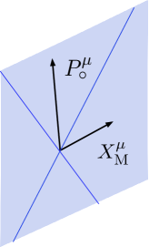
Figure 3: M

-plane spanned by $P_{\circ}^{\mu}$ and $X_{{\rm M}}^{\mu}$

The conserved center-of-mass momentum $P_{\circ}^{\mu}$ must be time-like (including a possible special case of light-like limit), $P_{\circ}^{2}<0$. Due to the Gauss constraint (46), this implies that $X_{{\rm M}}^{\mu}$ is a (conserved) space-like vector. Thus given an initial condition, we are automatically specifying a conserved two-dimensional plane spanned by $P_{\circ}^{\mu}$ and $X_{{\rm M}}^{\mu}$ in the Minkowski spacetime. In the following, we call this plane “M-plane” for convenience. In fixing the gauge for higher symmetries, the M-plane will play a preferential role, in the sense that there are no local physical degrees of freedom living solely on the M-plane. The emergence of preferential frame is essentially the same as in any Lorentz covariant formulation of particles in configuration space: recall that, given any state in a many-body system, we have a particular preferential frame, namely, the center-of-mass frame, where all of the spatial components of $P_{\circ}^{\mu}$ vanish. Namely, the preferential frames appear whenever we consider a particular state of particles, which specifies a particular configuration of particles. Only difference in our case is that there are two vectors, one time-like and the other space-like, instead of one time-like vector in cases of the usual many-body systems. Covariance in the configuration space of particles is guaranteed by the existence of generators of Lorentz transformation which operate in the space of states and satisfy the correct Lorentz algebra.

We will shortly see that the conserved auxiliary vector $X_{{\rm M}}^{\mu}$ plays a fundamental role of fixing M-theory scales as reviewed in the first part of this lecture. It also plays a crucial role in realizing supersymmetry in a most economical manner in our covariant formulation of Matrix theory.

10 The action of covariantized Matrix theory: bosonic part

Now we are in a position to write down the (bosonic part of the) action of our covariant Matrix theory:

$$A_{{\rm boson}} =\int d\tau\Bigl{[}P_{\circ}\cdot\frac{DX_{\circ}}{D\tau}+P_{{\rm M}}\cdot\frac{dX_{{\rm M}}}{d\tau}+{\rm Tr}\Bigl{(}\hat{\boldsymbol{P}}\cdot\frac{D\hat{\boldsymbol{X}}}{D\tau}\Bigr{)}$$

$$-\frac{e}{2N}P_{\circ}^{2}-\frac{e}{2}\,{\rm Tr}(\hat{\boldsymbol{P}}-P_{\circ}\boldsymbol{K})^{2}+\frac{e}{12}\bigl{<}[X^{\mu},X^{\nu},X^{\sigma}][X_{\mu},X_{\nu},X_{\sigma}]\bigr{>}\Bigr{]}.$$ (47)

The relative normalization between the kinetic momentum part and the last potential term is actually arbitrary, since it can be freely changed by redefinitions, $(X_{{\rm M}},P_{{\rm M}})\rightarrow(\rho X_{{\rm M}}^{\mu},\rho^{-1}P_{{\rm M}}^{\mu}),(B,\boldsymbol{B})\rightarrow\rho^{-1}(B,\boldsymbol{B})$, keeping other terms intact. This form of the bosonic action is characterized by the following four kinds of symmetries.

1. Local reparametrization invariance with respect to $\tau$.

2. Global translation invariance with respect to $X_{\circ}^{\mu}\rightarrow X_{\circ}^{\mu}+c^{\mu}$ and $P_{{\rm M}}^{\mu}\rightarrow P_{{\rm M}}^{\mu}+b^{\mu}$.

3. Global scaling symmetry (37) under $\tau\rightarrow\lambda^{2}\tau$.

4. Gauge symmetries under $\delta_{H}+\delta_{L}+\delta_{Y}+\delta_{w}$.

The local symmetries (1) and (4) give constraints. The Gauss constraints corresponding to the latter are already explicated in the previous section. The mass-shell condition corresponding to (1) is

$$P_{\circ}^{2}+{\cal M}_{{\rm boson}}^{2}\approx 0$$ (48)

with the effective squared-mass

$${\cal M}^{2}_{{\rm boson}}=N{\rm Tr}(\hat{\boldsymbol{P}}-P_{\circ}\boldsymbol{K})^{2}-\frac{N}{6}\bigl{<}[X^{\mu},X^{\nu},X^{\sigma}][X_{\mu},X_{\nu},X_{\sigma}]\bigr{>},$$ (49)

where the equality is valid only in conjunction with the Gauss-law constraints (43)$\sim$(46). This is indicated by the symbol $\approx$: remember that, when a variation of the ein-bein $e(\tau)$ is made, there are contributions from the covariant derivatives, involved in the generalized Poincaré invariant, which are linear with respect to all the gauge fields and consequently are linear combinations of the Gauss constraints. It is to be noted that in the large $N$ limit, we are interested in the regime where the spectrum of the squared mass is of order one and hence is independent of $N$ in the large $N$ limit.

That the effective mass is governed by the internal dynamics of this system is ensured by the fact that (49) involves only traceless matrix variables. It is easy to check that the equations of motion preserve the Gauss constraints, and hence they are consistently implemented. With respect to different roles of dynamical variables, it is to be noted that there is no inertial kinetic term for the “M-variables” $(X_{{\rm M}}^{\mu},P_{{\rm M}}^{\mu})$, due to the symmetry (2). Correspondingly, they do not participate to the dynamics actively: $X_{{\rm M}}^{\mu}$ is conserved, while $P_{{\rm M}}^{\mu}$ is passively determined by other variables through

$$\frac{DP_{{\rm M}}}{D\tau}=-\frac{\partial}{\partial_{{\rm M}\,\mu}}{\cal V}$$

where $-{\cal V}$ is the potential term in the above action and hence does not involve $P_{{\rm M}}^{\mu}$. The same can be said for the center-of-mass coordinate $X_{\circ}^{\mu}$ with respect to its passive character.

Now our next task is to confirm that this action leads to the same results as the light-front Matrix theory if we fix the gauge of higher-gauge symmetries appropriately and make explicit the condition of compactification. We can first choose the M-plane spanned by $P_{\circ}^{\mu}$ and $X_{{\rm M}}^{\mu}$. Since the former can be assumed to be time-like for generic states, while the latter then to be space-like due to the Gauss constraint (46), there is always a Lorentz frame where only non-zero components of these two conserved vectors are $P_{\circ}^{0},P_{\circ}^{10}$ and $X_{{\rm M}}^{0},X_{{\rm M}}^{10}$, respectively. Thus the M-plane is described by the light-like components $P_{\circ}^{\pm}\equiv P_{\circ}^{10}\pm P_{\circ}^{0},X_{{\rm M}}^{\pm}\equiv X_{{\rm M}}^{10}\pm X_{{\rm M}}^{0}$. We can then impose a gauge condition

$$\hat{\boldsymbol{X}}^{+}=0,$$ (50)

using the $\delta_{L}$-transformation, by which (45) is reduced to

$$0=P_{\circ}^{+}\hat{\boldsymbol{X}}^{-}+P_{\circ}^{-}\hat{\boldsymbol{X}}^{+}=P_{\circ}\hat{\boldsymbol{X}}^{-}\quad\Rightarrow\hat{\boldsymbol{X}}^{-}=0$$ (51)

since $P^{+}_{\circ}\neq 0$ due to our assumption that $P_{\circ}^{\mu}$ is time-like. With respect to $\delta_{Y}$-transformations, we choose $\boldsymbol{K}=0$ as discussed in the previous section. Then the first-order equations of motion allow us to express the light-like components of the matrix momentum as

$$\hat{\boldsymbol{P}}^{\pm}=\frac{1}{e}\frac{d\hat{\boldsymbol{X}}^{\pm}}{d\tau}+i[\boldsymbol{A},\hat{\boldsymbol{X}}^{\pm}]-\boldsymbol{B}X^{\pm}_{{\rm M}}$$ (52)

which give

$$\boldsymbol{P}^{\pm}=-\boldsymbol{B}X^{\pm}_{{\rm M}}.$$

Then, from the Gauss constraint (44) we obtain

$$0=X_{{\rm M}}^{-}\cdot\hat{\boldsymbol{P}}\quad\Rightarrow\quad\boldsymbol{B}X_{{\rm M}}^{2}=0\quad\boldsymbol{B}=0\quad\Rightarrow\hat{\boldsymbol{P}}^{\pm}=0.$$ (53)

Thus all of the light-like traceless matrices vanish in this gauge choice. Consequently, the squared mass and the remaining Gauss constraint (43) reduce, respectively, to

$${\cal M}^{2}_{{\rm boson}}=N{\rm Tr}\Bigl{(}\hat{\boldsymbol{P}}_{i}^{2}-\frac{1}{2}X_{{\rm M}}^{2}[\boldsymbol{X}_{i},\boldsymbol{X}_{j}]^{2}\Bigr{)}=\hat{H},$$ (54)

$$[\boldsymbol{X}_{i},\boldsymbol{P}_{i}]=0,$$ (55)

which coincides with (9) of section 3, by identifying the Lorentz invariant length of the M-variable after recovering the original unit of length, as

$$X_{{\rm M}}^{2}=\frac{1}{\ell_{11}^{6}}$$ (56)

in terms of the fundamental scale of M-theory. This implies that the scaling symmetry is broken by this choice. We will discuss about the meaning of this later.

In this gauge, the equations of motion for the center-of-mass variables and for $X_{{\rm M}}$ are

$$P_{\circ}^{\pm}=N\Bigl{(}\frac{dX_{\circ}^{\pm}}{ds}-BX_{{\rm M}}^{\pm}\Bigl{)},\quad\frac{dP^{\pm}_{\circ}}{ds}=0,\quad\frac{dX_{{\rm M}}^{\pm}}{ds}=0,$$

where we defined the re-parametrization invariant time parameter $s$ by $ds=ed\tau$. By choosing the gauge condition $B=0$ for the $\delta_{w}$-transformation, we have the standard form

$$P_{\circ}^{\pm}=N\frac{dX_{\circ}^{\pm}}{ds},$$

or

$$X_{\circ}^{+}=\frac{P_{\circ}^{+}}{N}s.$$ (57)

It is compulsory to assume that the relation between the target time and the invariant proper time $s$ is independent of $N$, as it should be since the systems with different sizes of matrices can always be regarded as subsystems of larger systems with increasingly larger $N$. Otherwise, we cannot consistently decompose a given system as a composite of subsystems: time $\tau$ or $s$ must be common to subsystems which are all synchronized with a single global internal time, as we have stressed in the previous section as a premiss of our canonical approach using a single proper time. Thus we must have

$$P_{\circ}^{+}=\frac{2N}{R}$$ (58)

with $R$ being a constant parameter which is independent of $N$ but can be varied continuously for different choices of the Lorentz frame. This somewhat remarkable result is consistent with the light-front Matrix theory as an effective theory of D0-branes where all D0-branes are supposed to have a single quantized unit of KK momentum in the limit of small $R$ identified with $R_{11}$.

Finally, we can derive an effective action for the remaining transverse variables by substituting

$$P_{\circ}^{-}=-\frac{\hat{H}}{P_{\circ}^{+}}$$

back into the original action. The result is, making conversion to the second-order formalism after eliminating the momenta,

$$A_{{\rm eff}}=\int dx^{+}\frac{1}{2R}{\rm Tr}\Bigl{(}\frac{D\hat{\boldsymbol{X}}^{i}}{Dx^{+}}\frac{D\hat{\boldsymbol{X}_{i}}}{Dx^{+}}+\frac{R^{2}}{2\ell_{11}^{6}}[\boldsymbol{X}_{i},\boldsymbol{X}_{j}][\boldsymbol{X}_{i},\boldsymbol{X}_{j}]\Bigr{)}$$

where we redefine the light-like time by $s=2Nx^{+}/P_{\circ}^{+}$ $(X_{\circ}=2x^{+}$).

The equations of motion for the center-of-mass coordinates and momenta does not prohibit us from imposing the BFSS condition

$$P_{\circ}^{10}=\frac{N}{R_{11}},$$

instead of the DLCQ scheme. In this case, we solve the mass-shell constraint as

$$P_{\circ}^{0}=\sqrt{(P_{\circ}^{10})^{2}+N{\rm Tr}\Bigl{(}\hat{\boldsymbol{P}}_{i}\cdot\hat{\boldsymbol{P}}_{i}-\frac{1}{2}X_{{\rm M}}^{2}[\boldsymbol{X}_{i},\boldsymbol{X}_{j}][\boldsymbol{X}_{i},\boldsymbol{X}_{j}]\Bigr{)}}.$$

Then the effective action is

$$A_{{\rm spat\,boson}}=\int dt\Bigl{[}{\rm Tr}\Bigl{(}\hat{\boldsymbol{P}}_{i}\frac{D\hat{\boldsymbol{X}}_{i}}{Dt}\Bigr{)}-P_{\circ}^{0}\Bigr{]}$$

with the time parameter $t=X_{\circ}^{0}=P_{\circ}^{10}s/N=s/R_{11}$. By eliminating $\hat{\boldsymbol{P}}_{i}$ in terms of the coordinate variables, we obtain the following Born-Infeld-like action:

$$A_{{\rm spat\,boson}}=-\int dt\,{\cal M}_{{\rm spat}}\sqrt{N}\Bigl{[}1-\frac{1}{N}{\rm Tr}\Bigl{(}\frac{D\hat{\boldsymbol{X}}_{i}}{Dt}\frac{D\hat{\boldsymbol{X}}_{i}}{Dt}\Bigr{)}\Bigr{]}^{1/2},$$

$${\cal M}_{{\rm spat}}\equiv\Bigl{[}\frac{N}{R_{11}^{2}}-\frac{1}{2\ell_{11}^{6}}{\rm Tr}\bigl{(}[\boldsymbol{X}_{i},\boldsymbol{X}_{j}][\boldsymbol{X}_{i},\boldsymbol{X}_{j}]\bigr{)}\Bigr{]}^{1/2}.$$

If we assume that the kinetic term, ${\rm Tr}\Bigl{(}\frac{D\hat{\boldsymbol{X}}_{i}}{Dt}\frac{D\hat{\boldsymbol{X}}_{i}}{Dt}\Bigr{)}$, and the potential term, ${\rm Tr}\bigl{(}[\boldsymbol{X}_{i},\boldsymbol{X}_{j}][\boldsymbol{X}_{i},\boldsymbol{X}_{j}]\bigr{)}$, are at most of order $O(1)$ with respect to $N$, the above effective action is approximated as

$$\int dt\,\frac{N}{R_{11}}\Bigl{[}-1+\frac{1}{2N}{\rm Tr}\Bigl{(}\frac{D\hat{\boldsymbol{X}}_{i}}{Dt}\frac{D\hat{\boldsymbol{X}}_{i}}{Dt}+\frac{R_{11}^{2}}{2\ell_{11}^{6}}[\boldsymbol{X}_{i},\boldsymbol{X}_{j}][\boldsymbol{X}_{i},\boldsymbol{X}_{j}]\Bigr{)}+O(\frac{1}{N^{2}})\Bigr{]}.$$

Of course, this is consistent with a natural expectation from our viewpoint on the relationship between the IMF and DLCQ schemes, discussed in section 3. On the other hand, our result shows that in the opposite limit $R_{11}\rightarrow\infty$ with fixed $N$, the system becomes a very peculiar and singular system which does not have standard kinetic terms.

At this juncture, let us consider the meaning of the violation of scaling symmetry, which is required in order to relate our system with light-front Matrix theory. Namely, the 11 dimensional Planck length emerges by specifying the value of $X_{{\rm M}}^{2}$ as an initial condition. This determines the coupling constant for the internal dynamics of the system. A natural interpretation of this situation seems that $X_{{\rm M}}^{2}$ defines a super-selection rule with respect to scaling transformations. Namely, once its value is fixed by initial condition, no superposition is allowed among different values of $X_{{\rm M}}^{2}$. The scale symmetry means that any two systems with different values of $X_{{\rm M}}^{2}$ are mapped into each other with a simple rescaling of dynamical variables. Thus all the different super-selection sectors actually describe essentially the same physics, apart from global scaling transformations. The initial condition just selects one of the continuously distributed super-selection sectors. In this sense, scale symmetry is spontaneously broken. On the other hand, scale symmetry signifies an important fact that our theory has one and only one fundamental length scale $\ell_{11}$ through spontaneous symmetry breaking.

It should be noted also that, even though states are not superposed between different values of invariant $X_{{\rm M}}^{2}$, states with different Lorentz components of $X_{{\rm M}}^{\mu}$ must be allowed to be superposed. That this is the case is seen, for instance, from the constraint (46), which in the light-like coordinates of the M-plane takes the form,

$$P_{\circ}^{-}=-\frac{P_{\circ}^{+}}{(X_{{\rm M}}^{+})^{2}}X_{{\rm M}}^{2}\qquad\mbox{or}\qquad P_{\circ}^{0}=\frac{P_{\circ}^{10}X_{{\rm M}}^{10}}{\sqrt{(X_{{\rm M}}^{10})^{2}-X_{{\rm M}}^{2}}}.$$

This implies that different states with different “energies”$P_{\circ}^{-}$ or $P_{\circ}^{10}$, in general, have different values $X_{{\rm M}}^{+}$ or $X_{{\rm M}}^{10}$, respectively. The states with different energies are certainly superposed in quantum dynamics, and hence also states with different values of these components of the M-variable with fixed $X_{{\rm M}}^{2}$ are in general superposed. Incidentally, these relations show that the light-like limit $P_{\circ}^{-}\rightarrow 0$ corresponds to a singular limit $X_{{\rm M}}^{+}\rightarrow\infty$ or $X_{{\rm M}}^{10}\rightarrow\infty$.

11 Supersymmetry

Now let us come to our last subject of this lecture. The question we have to ask is now whether and how our covariantized Matrix theory can have supersymmetry, which is also one of indispensable elements ensuring the compatibility of this system with eleven-dimensional gravity. One of obstacles in formulating supersymmetry in a covariant fashion is that we have to reduce the number of degrees of freedom associated with the fermion variables in 11 dimensions: a single Majonara fermion has 32 (real) components. If we suppose that supersymmetry is realized without spontaneous symmetry breaking, the number of physical degrees of freedom must match between bosonic and fermionic degrees of freedom. The bosonic coordinate degrees of freedom is $11-2-1=8$ for each real components of matrices in our system: $-2$ corresponds to higher gauge symmetry and $-1$ to the ordinary SU($N$) gauge symmetry. Thus, 32 of the Majorana fermion must be reduced to $2\times 8=16$. In the classical theory of supermembrane, this reduction is made due to the presence of a fermionic gauge symmetry, the so-called $\kappa$-symmetry. It is also the case of manifestly covariant formulations of superstrings in 10 dimensions. Using this $\kappa$-symmetry, we can put a gauge condition on fermions, achieving the required reduction. In the same vein, we may try to find some extension of $\kappa$-like fermionic gauge symmetry in our system. However, for our purpose it is sufficient if we have some way of imposing condition of reduction directly without violating Lorentz covariance. In that case, the existence of such fermionic gauge symmetry is not a necessary prerequisite for a covariant formulation of supersymmetry. In this lecture, we take this standpoint. Of course, this does not mean that the fermionic gauge symmetry is impossible: at least from esthetic viewpoint, such a symmetry would be still desirable, though from a practical viewpoint it may neither be necessary nor useful. One of the reasons for our standpoint is that in the case of fermionic variables, it is impossible to separate them into the coordinate and momentum variables in a covariant fashion, since they are inextricably mixed under Lorentz transformations, corresponding to their first-order nature of the dynamics of fermions. This feature necessarily leads to second-class constraints in the canonical formalism, and compels us to assign the same transformation law for all spinor components on an equal footing, which can be satisfied only for the usual SU($N$) gauge transformation.

We denote the fermionic Majonara variable by $\Theta_{\circ}$ and $\boldsymbol{\Theta}$ : the former is the fermionic partner to the center-of-mass bosonic variables $(X_{\circ}^{\mu},P_{\circ}^{\mu})$. The latter is a traceless hermitian matrix whose real components are Majorana fermions separately. For notational brevity, we suppress the $\hat{\,\,}$ symbol for the fermion traceless matrix. One basic assumption corresponding to our standpoint explained above is that there is no fermionic counterpart for the bosonic M-variables $(X_{{\rm M}}^{\mu},P_{{\rm M}}^{\mu})$. This implies that the fermionic variables do not subject to higher-gauge transformations:

$$\delta_{HL}\Theta=\delta_{HY}\Theta=\delta_{H}\Theta=(0,i\sum_{r}[F^{(r)},G^{(r)},\Theta])=(0,\delta_{H}\boldsymbol{\Theta}),$$

$$\delta_{H}\boldsymbol{\Theta}=i[\boldsymbol{H},\boldsymbol{\Theta}]$$ (59)

Consequently, as for the invariants involving only fermionic variables, we can adopt usual trace of product of matrices. For expressing invariants involving both fermionic and bosonic variables, 3-bracket notation is still necessary and useful.

We first treat the center-of-mass part, which can be regarded as if it is a single massive relativistic particle. It is then natural to define its action just by adopting the standard formulation of a single relativistic superparticle,[18] as

$$\int d\tau P_{\circ\,\mu}\bar{\Theta}_{\circ}\Gamma^{\mu}\frac{d\Theta_{\circ}}{d\tau},$$ (60)

which is obtained from the bosonic Poincaré invariant by a replacement,

$$\frac{dX^{\mu}_{\circ}}{d\tau}\rightarrow\frac{dX^{\mu}_{\circ}}{d\tau}+\bar{\Theta}_{\circ}\Gamma^{\mu}\frac{d\Theta_{\circ}}{d\tau}.$$

Corresponding to this origin of the fermionic action, the center-of-mass system is supersymmetric under

$$\delta_{\varepsilon}\Theta_{\circ}=-\varepsilon,\quad\delta_{\varepsilon}X_{\circ}^{\mu}=\bar{\varepsilon}\Gamma^{\mu}\Theta_{\circ},\quad\delta_{\varepsilon}P_{\circ}^{\mu}=0,$$ (61)

satisfying

$$\delta_{\varepsilon}\Bigl{(}\frac{dX^{\mu}_{\circ}}{d\tau}+\bar{\Theta}_{\circ}\Gamma^{\mu}\frac{d\Theta_{\circ}}{d\tau}\Bigr{)}=0,$$

with a constant $\varepsilon$. $\Gamma^{\mu}$’s are 11 dimensional Dirac matrices in the Majorana representation. This transformation is not a linear transformation: it is characterized by the shift-type transformation of $\Theta_{\circ}$, signifying that $\Theta_{\circ}$ is super-coordinate accompanying the bosonic coordinates $X_{\circ}^{\mu}$. The bosonic M-variables and all traceless matrix variables are inert under this supersymmetry. Note that the scaling transformation for the fermionic variables are $\Theta_{\circ}\rightarrow\lambda^{1/2}\Theta_{\circ},\varepsilon\rightarrow\lambda^{1/2}\varepsilon$, and also that the $\delta_{w}$ symmetry of the bosonic part is not spoiled: it is still valid with the covariant derivative $DX_{\circ}^{\mu}/D\tau$ and the conservation law of $X_{{\rm M}}^{\mu}$. Thus the Gauss law (46) is intact, being invariant under the above supersymmetry transformation.

The equation of motion for $\Theta_{\circ}$ is

$$P_{\circ}\cdot\Gamma\frac{d\Theta_{\circ}}{d\tau}=0$$

which for generic time-like $P_{\circ}^{\mu}$ leads to the conservation law

$$\frac{d\Theta_{\circ}}{d\tau}=0.$$

Thus the on-shell equations of motion for bosonic center-of-mass coordinates are not modified.

The generic quantum states consist of fundamental massive super-multiplet of dimensions $2^{16}$. In the special limit of light-like center-of-mass satisfying $P_{\circ}^{2}=0$, it is well known that this system has a local fermionic symmetry called Siegel symmetry which is the origin of more general $\kappa$-symmetry of string and membrane theories.

$$\delta_{\kappa}\Theta_{\circ}=P_{\circ}\cdot\Gamma\kappa,\quad\delta_{\kappa}X_{\circ}^{\mu}=-\bar{\Theta}_{\circ}\Gamma^{\mu}\delta_{\kappa}\Theta_{\circ},$$

where $\kappa=\kappa(\tau)$ is an arbitrary Majorana spinor function. This allows one to eliminate a half of components of $\Theta_{\circ}$ adjoined with a suitable redefinition of $X_{\circ}^{\mu}$. Thus, a massless graviton multiplet consists of $2^{16/2}=2^{8}$ states. But in the present case, we are in general dealing with many-body states of such gravitons which obeys the massive representations, where $-P_{\circ}^{2}>0$.

Now we turn to traceless matrix part, describing the internal dynamics of the system. Unlike the center-of-mass case, supersymmetry transformations of traceless matrices are expected to start from a linear form without shift-type contributions, but with possible nonlinear corrections of higher orders. As for the bosonic coordinates, we start from

$$\delta_{\epsilon}\hat{\boldsymbol{X}}^{\mu}=\bar{\epsilon}\Gamma^{\mu}\boldsymbol{\Theta},$$ (62)

where we have different symbol $\epsilon$ for the fermionic parameter of transformation, in order to keep in mind that this transformation is independent of the previous one for the center-of-mass system. We call this supersymmetry dynamical supersymmetry. For this type of transformations to be successfully formulated, as we have discussed in the beginning of this section, we have to impose some constraints, thereby which the degrees of freedom match between bosonic and fermionic sides. This necessarily comes about by requiring that supersymmetry transformation should keep the bosonic Gauss constraints consistently. If we assume naturally that $P_{\circ}^{\mu}$ and $X_{{\rm M}}^{\mu}$ are inert under dynamical super transformation, the constraints, (44) and (45), require

$$X_{{\rm M}}\cdot\delta_{\epsilon}\hat{\boldsymbol{P}}=0,\quad P_{\circ}\cdot\delta_{\epsilon}\hat{\boldsymbol{X}}=0,$$ (63)

respectively. There is a natural projection condition suitable for our demand, due to the existence of the M-plane in the bosonic sector. We define (real) projection operators

$$P_{\pm}\equiv\frac{1}{2}(1\pm\Gamma_{\circ}\Gamma_{{\rm M}}),\quad P_{\pm}^{2}=P_{\pm},\quad P_{\pm}P_{\mp}=0$$ (64)

where

$$\Gamma_{{\rm M}}\equiv\frac{X_{{\rm M}}\cdot\Gamma}{\sqrt{X_{{\rm M}}^{2}}},\quad\Gamma_{\circ}\equiv\frac{P_{\circ}\cdot\Gamma}{\sqrt{-P_{\circ}^{2}}}$$

are conserved and Lorentz invariant, satisfying

$$\Gamma_{{\rm M}}\Gamma_{\circ}+\Gamma_{\circ}\Gamma_{{\rm M}}=0,\quad\Gamma_{{\rm M}}^{2}=1,\quad\Gamma_{\circ}^{2}=-1,\quad(\Gamma_{\circ}\Gamma_{{\rm M}})^{2}=1,$$

$$P_{+}\Gamma_{{\rm M}}=\Gamma_{{\rm M}}P_{-},\,\,P_{+}\Gamma_{\circ}=\Gamma_{\circ}P_{-},\quad P_{\pm}\Gamma_{i}=\Gamma_{i}P_{\pm},$$ (65)

where $i$ denotes SO(9) directions in any (orthogonal) basis, being transverse to the M-plane. For the validity of these relations, it is crucial to use the orthogonality of two conserved vectors $P_{\circ}^{\mu}$ and $X_{{\rm M}}^{\mu}$, namely the Gauss constraint (46) associated with $\delta_{w}$-gauge transformations. Thus it should be kept in mind that the dynamical supersymmetry is satisfied in each sector with definite values of these conserved and mutually orthogonal vectors.

The last relation (65) shows that we can clearly separate the directions between those (called “longitudinal”) along the M-plane and those (called “transversal”) orthogonal to the M-plane. This is precisely what we need in order to meet our requirements (63). We introduce the projection conditions as

$$P_{-}\boldsymbol{\Theta}=\boldsymbol{\Theta},\,\,P_{+}\boldsymbol{\Theta}=0,\quad\mbox{(or \,\, equivalently \,\, $\bar{\boldsymbol{\Theta}}P_{+}=\bar{\Theta},\,\,\bar{\boldsymbol{\Theta}}P_{-}=0$)}$$ (66)

together with the opposite projection on $\epsilon$,

$$P_{+}\epsilon=\epsilon,\,\,P_{-}\epsilon=0,\quad\mbox{(or \,\, equivalently \,\, $\bar{\epsilon}P_{-}=\bar{\epsilon},\,\,\bar{\epsilon}P_{+}=0$)}.$$ (67)

This eliminates a half of 32 Majorana components, as required. Using the postulate (62), we can confirm that the second of (63) is indeed satisfied:

$$\bar{\epsilon}P_{\circ}\cdot\Gamma\boldsymbol{\Theta}=\bar{\epsilon}P_{-}(P_{\circ}\cdot\Gamma)P_{-}\boldsymbol{\Theta}=\bar{\epsilon}(P_{\circ}\cdot\Gamma)P_{+}P_{-}\boldsymbol{\Theta}=0,$$ (68)

and also

$$\bar{\epsilon}X_{{\rm M}}\cdot\Gamma\boldsymbol{\Theta}=\bar{\epsilon}P_{-}(X_{{\rm M}}\cdot\Gamma)P_{-}\boldsymbol{\Theta}=\bar{\epsilon}X_{{\rm M}}\cdot\Gamma P_{+}P_{-}\boldsymbol{\Theta}=0,$$ (69)

while

$$\bar{\epsilon}\Gamma_{i}\boldsymbol{\Theta}=\bar{\epsilon}P_{-}\Gamma_{i}P_{-}\boldsymbol{\Theta}=\bar{\epsilon}\Gamma_{i}P_{-}\boldsymbol{\Theta}=\bar{\epsilon}P_{-}\Gamma_{i}\boldsymbol{\Theta}$$ (70)

can be non-vanishing for all $i$’s, transverse to both $P_{\circ}^{\mu}$ and $X_{{\rm M}}^{\mu}$. Thus as expected, the dynamical supersymmetry is effective only for the spacetime directions which are transverse to the M-plane. This is natural, since as we have seen clearly in the previous section that internal dynamics is associated entirely to the transverse variables.

In fact, if we adopt the light-like Lorentz frame which we have introduced in discussing gauge fixing in the previous section, the projection condition is equivalent to the ordinary light-cone condition for fermionic matrices: we can rewrite (66) by multiplying $\Gamma_{\circ}$ on both sides, as

$$(\Gamma_{\circ}-\Gamma_{{\rm M}})\boldsymbol{\Theta}=0,$$

which reduces to

$$0 =\frac{1}{2\sqrt{-P_{\circ}^{2}}}\Bigl{(}P_{\circ}^{+}\Gamma^{-}+P_{\circ}^{-}\Gamma^{+}-\frac{\sqrt{-P_{\circ}^{+}P_{\circ}^{-}}}{\sqrt{X_{{\rm M}}^{2}}}(X_{{\rm M}}^{+}\Gamma^{-}+X_{{\rm M}}^{-}\Gamma^{+})\Bigr{)}\boldsymbol{\Theta}$$

$$=\frac{1}{2\sqrt{-P_{\circ}^{2}}}\Bigl{(}P_{\circ}^{+}\Gamma^{-}+P_{\circ}^{-}\Gamma^{+}-\frac{P_{\circ}^{+}}{X_{{\rm M}}^{+}}(X_{{\rm M}}^{+}\Gamma^{-}+\frac{X_{{\rm M}}^{2}}{X_{{\rm M}}^{+}}\Gamma^{+})\Bigr{)}\boldsymbol{\Theta}$$

$$=-\sqrt{-\frac{P_{\circ}^{-}}{P_{\circ}^{+}}}\Gamma^{+}\boldsymbol{\Theta}.$$

We will give full transformation laws for dynamical supersymmetry, after showing the total supersymmetric action involving both bosonic and fermionic variables in the next section.

12 The total supersymmetric action

The total action is

$$A=A_{{\rm boson}}+A_{{\rm fermion}},$$ (71)

where $A_{{\rm boson}}$ is given by (47) and

$$A_{{\rm fermion}}= \int d\tau\,\Bigl{[}\bar{\Theta}_{\circ}P_{\circ}\cdot\Gamma\frac{d\Theta_{\circ}}{d\tau}+\frac{1}{2}{\rm Tr}\Bigl{(}\bar{\boldsymbol{\Theta}}\Gamma_{\circ}\frac{D\boldsymbol{\Theta}}{D\tau}\Bigr{)}$$

$$-e\frac{i}{4}\bigl{<}\bar{\Theta},\Gamma_{\mu\nu}[X^{\mu},X^{\nu},\Theta]\bigr{>}\Bigr{]},$$ (72)

$$\bigl{<}\bar{\Theta},\Gamma_{\mu\nu}[X^{\mu},X^{\nu},\Theta]\bigr{>}$$

$$=2\sqrt{X_{{\rm M}}^{2}}{\rm Tr}\bigl{(}\bar{\boldsymbol{\Theta}}\Gamma_{\circ}\Gamma_{i}[\boldsymbol{X}_{i},\boldsymbol{\Theta}]\bigr{)}=2\sqrt{X_{{\rm M}}^{2}}{\rm Tr}\bigl{(}\bar{\boldsymbol{\Theta}}\Gamma_{\circ}\Gamma_{\mu}[\boldsymbol{X}^{\mu},\boldsymbol{\Theta}]\bigr{)}.$$ (73)

The last expression of the femionic potential terms is derived by using

$$\bigl{<}\bar{\Theta},\Gamma_{\mu\nu}[X^{\mu},X^{\nu},\Theta]\bigr{>}=2{\rm Tr}\bigl{(}\bar{\boldsymbol{\Theta}}\Gamma_{\mu\nu}X_{{\rm M}}^{\mu}[\boldsymbol{X}^{\nu},\boldsymbol{\Theta}]\bigr{)}$$

which is rewritten as above due to the projection condition $\Gamma_{{\rm M}}\boldsymbol{\Theta}=\Gamma_{\circ}\boldsymbol{\Theta}$. Here it is to be noted that the normalizations of the center-of-mass part and of the traceless matrix part is different, such that, in the latter, the scaling dimensions of $\boldsymbol{\Theta}$ is chosen to be zero, while that of the susy parameter $\epsilon$ is 1, in order to simplifying the expressions. The full dynamical supersymmetry transformations are

$$\delta_{\epsilon}\hat{\boldsymbol{X}}^{\mu}=\bar{\epsilon}\Gamma^{\mu}\boldsymbol{\Theta},$$ (74)

$$\delta_{\epsilon}\hat{\boldsymbol{P}}_{\mu}=i\sqrt{X_{{\rm M}}^{2}}\,\bigl{[}\bar{\boldsymbol{\Theta}}\Gamma_{\mu\nu}\epsilon,\tilde{\boldsymbol{X}}^{\nu}],\quad\delta_{\epsilon}\boldsymbol{K}=0,$$ (75)

$$\delta_{\epsilon}\boldsymbol{\Theta}=P_{-}\bigl{(}\Gamma_{\circ}\Gamma_{\mu}\hat{\boldsymbol{P}}^{\mu}\epsilon-\frac{i}{2}\sqrt{X_{{\rm M}}^{2}}\,\Gamma_{\circ}\Gamma_{\mu\nu}\epsilon[\tilde{\boldsymbol{X}}^{\mu},\tilde{\boldsymbol{X}}^{\nu}]\bigr{)},$$ (76)

$$\delta_{\epsilon}\boldsymbol{A}=\sqrt{X_{{\rm M}}^{2}}\,\bar{\boldsymbol{\Theta}}\epsilon,$$ (77)

$$\delta_{\epsilon}\boldsymbol{B}=i\bigl{(}X_{{\rm M}}^{2}\bigr{)}^{-1}[\delta_{\epsilon}\boldsymbol{A},X_{{\rm M}}\cdot\boldsymbol{X}],$$ (78)

$$\delta_{\epsilon}\boldsymbol{Z}=i(P_{\circ}^{2})^{-1}[\delta_{\epsilon}\boldsymbol{A},P_{\circ}\cdot\boldsymbol{P}]$$

$$\hskip 19.91684pt+\frac{X_{{\rm M}}^{2}}{2P_{\circ}^{2}}([\delta_{\epsilon}\boldsymbol{X}^{\mu},[P_{\circ}\cdot\boldsymbol{X},\boldsymbol{X}_{\mu}]]+[\boldsymbol{X}^{\mu},[P_{\circ}\cdot\boldsymbol{X},\delta_{\epsilon}\boldsymbol{X}_{\mu}]]),$$ (79)

with

$$\tilde{\boldsymbol{X}}^{\mu}=\boldsymbol{X}^{\mu}-\frac{1}{X_{{\rm M}}^{2}}X_{{\rm M}}^{\mu}(\boldsymbol{X}\cdot X_{{\rm M}})-\frac{1}{P_{\circ}^{2}}P_{\circ}^{\mu}(\boldsymbol{X}\cdot P_{\circ}).$$ (80)

The existence of gauge fields is crucial for dynamical supersymmetry. It is easy to check that the transformation law (75) for the momentum matrix satisfies the first of our requirements (63).

There is a caveat here : in deriving these transformation laws, we have to assume the conservation laws for $P_{\circ}^{\mu}$ and $X_{{\rm M}}^{\mu}$ which are actually resulting only after using the equations of motion for these variables, together with the Gauss law (46), as we have already alluded to in the previous section. I would like to refer the reader to my original paper[21] for a derivation of these results.

With this caveat, we can also express the supersymmetry transformation laws in a form of the algebra of supersymmetry generators, using Dirac bracket which takes into account the primary second-class constraint for the fermion matrices. Denoting the canonical conjugate to $\boldsymbol{\Theta}$ by $\boldsymbol{\Pi}$, the primary second-class constraint for the traceless fermion matrices is

$$\boldsymbol{\Pi}+\frac{1}{2}\bar{\boldsymbol{\Theta}}\Gamma_{\circ}=0,\quad(\boldsymbol{\Pi}P_{-}=\boldsymbol{\Pi})$$ (81)

which satisfy the Poisson bracket algebra expressed in a component form

$$\{\Pi_{\alpha}^{A}+\frac{1}{2}(\bar{\Theta}^{A}\Gamma_{\circ})_{\alpha},\Pi_{\beta}^{B}+\frac{1}{2}(\bar{\Theta}^{A}\Gamma_{\circ})_{\beta}\}_{{\rm P}}=(\Gamma^{0}\Gamma_{\circ}P_{-})_{\alpha\beta}\delta^{AB},$$ (82)

where we have denoted the spinor indices by $\alpha,\beta,\ldots,$. The indices $A,B,\ldots$ refer to the components with respect to the traceless spinor matrices using an hermitian orthogonal basis $\boldsymbol{\Theta}=\sum_{A}\Theta^{A}\boldsymbol{T}^{A}$ satisfying ${\rm Tr}(\boldsymbol{T}^{B}\boldsymbol{T}^{B})=\delta^{AB}$ of SU($N$) algebra. The non-trivial Dirac brackets for traceless matrices are then

$$\{\Theta^{A}_{\alpha},\bar{\Theta}^{B}_{\beta}\}_{{\rm D}}=-(P_{-}\Gamma_{\circ})_{\alpha\beta}\delta^{AB},\quad$$ (83)

$$\{\hat{X}^{A}_{\mu},\hat{P}^{B}_{\nu}\}_{{\rm D}}=\eta_{\mu\nu}\delta^{AB}.$$ (84)

Then the supercharge defined by

$${\cal Q}=P_{-}{\rm Tr}(\tilde{\hat{\boldsymbol{P}}}_{\mu}\Gamma^{\mu}\boldsymbol{\Theta}-\frac{i}{2}\sqrt{X_{{\rm M}}^{2}}[\tilde{\boldsymbol{X}}^{\mu},\tilde{\boldsymbol{X}}^{\nu}]\Gamma_{\mu\nu}\boldsymbol{\Theta})$$ (85)

with

$$\tilde{\hat{\boldsymbol{P}}}^{\mu}=\hat{\boldsymbol{P}}^{\mu}-\frac{1}{X_{{\rm M}}^{2}}X_{{\rm M}}^{\mu}(\hat{\boldsymbol{P}}\cdot X_{{\rm M}})-\frac{1}{P_{\circ}^{2}}P_{\circ}^{\mu}(\hat{\boldsymbol{P}}\cdot P_{\circ}),$$ (86)

satisfies

$$\{\bar{\epsilon}{\cal Q},\hat{\boldsymbol{X}}^{\mu}\}_{{\rm D}} =-\bar{\epsilon}\Gamma^{\mu}\boldsymbol{\Theta},$$ (87)

$$\{\bar{\epsilon}{\cal Q},\hat{\boldsymbol{P}}_{\mu}\}_{{\rm D}} =-i\sqrt{X_{{\rm M}}^{2}}[\bar{\epsilon}\Gamma_{\mu\nu}\boldsymbol{\Theta},\tilde{\boldsymbol{X}}^{\nu}]=i\sqrt{X_{{\rm M}}^{2}}[\bar{\boldsymbol{\Theta}}\Gamma_{\mu\nu}\epsilon,\tilde{\boldsymbol{X}}^{\nu}],$$ (88)

$$\{\bar{\epsilon}{\cal Q},\boldsymbol{\Theta}\}_{{\rm D}} =-P_{-}\bigl{(}\Gamma_{\circ}\Gamma_{\mu}\hat{\boldsymbol{P}}^{\mu}\epsilon-\frac{i}{2}\sqrt{X_{{\rm M}}^{2}}\,\Gamma_{\circ}\Gamma_{\mu\nu}\epsilon[\tilde{\boldsymbol{X}}^{\mu},\tilde{\boldsymbol{X}}^{\nu}]\bigr{)}.$$ (89)

The algebra of supercharge is

$$\{\bar{\epsilon}_{1}{\cal Q},\bar{\epsilon}_{2}{\cal Q}\}_{{\rm D}} =-2(\bar{\epsilon_{1}}\Gamma_{\circ}\epsilon_{2}){\rm Tr}\Bigl{(}\frac{1}{2}\tilde{\hat{\boldsymbol{P}}}^{2}-\frac{1}{4}X_{{\rm M}}^{2}[\tilde{\boldsymbol{X}}^{\mu},\tilde{\boldsymbol{X}}^{\nu}][\tilde{\boldsymbol{X}}_{\mu},\tilde{\boldsymbol{X}}_{\nu}]$$

$$+\frac{i}{2}\sqrt{X_{{\rm M}}^{2}}(\bar{\boldsymbol{\Theta}}\Gamma_{\circ}\Gamma_{\mu}[\boldsymbol{X}^{\mu},\boldsymbol{\Theta}])\Bigr{)}$$

$$+2(\bar{\epsilon}_{1}\Gamma_{\circ}\Gamma_{\mu}\epsilon_{2})\sqrt{X_{{\rm M}}^{2}}{\rm Tr}\bigl{(}i\tilde{\boldsymbol{X}}^{\mu}[\tilde{\boldsymbol{X}}^{\nu},\tilde{\boldsymbol{P}}_{\nu}]-\frac{1}{2}i\tilde{\boldsymbol{X}}^{\mu}[\boldsymbol{\Theta},\Gamma^{0}\Gamma_{\circ}\boldsymbol{\Theta}]_{+}\bigr{)}.$$ (90)

This result can be regarded just to be a covariantized version of the results well-known in the light-front Matrix theory. In our context, this shows that, since the first part on the r.h.side is proportional to the effective squared mass of this system up to a field-dependent SU($N$) gauge transformation exhibited in the second part, the commutator $[\delta_{\epsilon_{1}},\delta_{\epsilon_{2}}]$ induces an infinitesimal translation $s\rightarrow s-2\bar{\epsilon}_{1}\Gamma_{\circ}\epsilon_{2}$ of the invariant proper-time parameter $s$. This of course reflects the fact that the dynamical supersymmetry is associated with the internal dynamics of this system. On the other hand, the supersymmetry, represented by $\delta_{\varepsilon}$, of the center-of-mass system does not induce the translation of the proper time: instead, it directly induces the translation of the center-of-mass coordinate $X_{\circ}^{\mu}$ without any shift of the proper time parameter. Because of this, it is appropriately called to be “kinematical” supersymmetry. A similar nature of the composition of kinematical and dynamical supersymmetries had already been apparent in the light-like formulation. It becomes more evident in our covariant formulation, due to manifestly different roles played by the internal proper time parameter and by the coordinates of target spacetime.

That the matrix gauge fields are transformed in realizing dynamical supersymmetry is related to the fact that the mass-shell condition must be understood in conjunction with the Gauss law constraints, as we have emphasized in the purely bosonic case. The full action gives the following expressions for Gauss constraints of matrix type, apart from (46):

$$\boldsymbol{G}_{A}\equiv i[\boldsymbol{X}^{\mu},\boldsymbol{P}_{\mu}]-\frac{i}{2}[\boldsymbol{\Theta},\Gamma^{0}\Gamma_{\circ}\boldsymbol{\Theta}]_{+}\approx 0,$$ (91)

$$\boldsymbol{G}_{B}\equiv X_{{\rm M}}\cdot\hat{\boldsymbol{P}}\approx 0,$$ (92)

$$\boldsymbol{G}_{Z}\equiv P_{\circ}\cdot\hat{\boldsymbol{X}}=0,\quad P_{\circ}\cdot\hat{\boldsymbol{P}}=0$$ (93)

where in the last line we also wrote down the constraint derived as the equation of motion for the auxiliary field $\boldsymbol{K}$ in the gauge $\boldsymbol{K}=0$. It is easily seen that all of these constraints are invariant under supersymmetry transformation:

$$\delta_{\epsilon}\boldsymbol{G}_{A}=0,\quad\delta_{\epsilon}\boldsymbol{G}_{B}=0,\quad\delta_{\epsilon}\boldsymbol{G}_{Z}=0,\quad\delta_{\epsilon}(P_{\circ}\cdot\hat{\boldsymbol{P}})=0.$$

On the other hand, the squared mass is

$${\cal M}^{2} \approx N{\rm Tr}(\hat{\boldsymbol{P}}\cdot\hat{\boldsymbol{P}})-\frac{N}{6}\bigl{<}[X^{\mu},X^{\nu},X^{\sigma}],[X_{\mu},X_{\nu},X_{\sigma}]$$

$$+i\frac{N}{2}\bigl{<}\bar{\Theta},\Gamma_{\mu\nu}[X^{\mu},X^{\nu},\Theta]\bigr{>}$$

$$=N{\rm Tr}\Bigl{(}\hat{\boldsymbol{P}}\cdot\hat{\boldsymbol{P}}-\frac{1}{2}\bigl{(}X_{{\rm M}}^{2}[\boldsymbol{X}^{\nu},\boldsymbol{X}^{\sigma}][\boldsymbol{X}_{\nu},\boldsymbol{X}_{\sigma}]$$

$$-2[X_{{\rm M}}\cdot\boldsymbol{X},\boldsymbol{X}^{\nu}][X_{{\rm M}}\cdot\boldsymbol{X},\boldsymbol{X}_{\nu}]\bigr{)}+i\bar{\boldsymbol{\Theta}}\Gamma_{\mu\nu}X_{{\rm M}}^{\mu}[\boldsymbol{X}^{\nu},\boldsymbol{\Theta}]\Bigr{)}$$ (94)

which is an equality under the above Gauss constraints, and is not itself invariant against the dynamical super transformations, satisfying

$$\delta_{\epsilon}\Bigl{(}{\rm Tr}(\boldsymbol{A}\boldsymbol{G}_{A}-\hat{\boldsymbol{B}}\boldsymbol{G}_{B}+\boldsymbol{Z}\boldsymbol{G}_{Z})-\frac{1}{2N}{\cal M}^{2}\Bigr{)}=0.$$ (95)

It is therefore indispensable to take into account the Gauss constraints in treating the mass-shell condition, which itself is invariant against both kinematical and dynamical supersymmetry transformations. Of course, the invariance of the mass-shell condition under the kinematical supersymmetry is ensured by $\delta_{\varepsilon}P_{\circ}^{\mu}=\delta_{\varepsilon}X_{{\rm M}}^{\mu}=0$.

In the light-front gauge, the mass-shell condition reduces to

$$P_{\circ}^{2}+{\cal M}_{{\rm lf}}^{2}\approx 0$$

$${\cal M}_{{\rm lf}}^{2}\equiv N{\rm Tr}\bigl{(}\hat{\boldsymbol{P}}^{i}\hat{\boldsymbol{P}}^{i}-\frac{1}{2}X_{\rm M}^{2}[\boldsymbol{X}_{i},\boldsymbol{X}_{j}][\boldsymbol{X}_{i},\boldsymbol{X}_{j}]+i\sqrt{X_{{\rm M}}^{2}}\boldsymbol{\Theta}\Gamma_{i}[\boldsymbol{X}_{i},\boldsymbol{\Theta}]\bigr{)}.$$

Here we made a rescaling of the fermion matrix in order to fit it into the usual normalization of the light-front matrix theory,

$$\boldsymbol{\Theta}\rightarrow\sqrt{2}\Bigl{(}-\frac{P^{+}_{\circ}}{P_{\circ}^{-}}\Bigr{)}^{-1/4}\boldsymbol{\Theta}.$$ (96)

By repeating the procedure of deriving effective action in the bosonic case, we obtain the following effective action for the light-front theory in the first-order form:

$$A_{{\rm lf}}=\int ds\,\Bigl{[}{\rm Tr}\Bigl{(}\hat{\boldsymbol{P}}_{i}\frac{D\hat{\boldsymbol{X}}_{i}}{Ds}+\frac{1}{2}\boldsymbol{\Theta}\frac{D\boldsymbol{\Theta}}{Ds}\Bigr{)}-\frac{1}{2N}{\cal M}_{{\rm lf}}^{2}\Bigr{]}.$$ (97)

In the case of the IMF gauge, the corresponding result is

$$A_{{\rm spat}}=\int ds\Bigl{[}{\rm Tr}\Bigl{(}\hat{\boldsymbol{P}}_{i}\frac{D\hat{\boldsymbol{X}}_{i}}{Ds}+\frac{1}{2}\boldsymbol{\Theta}\frac{D\boldsymbol{\Theta}}{Ds}\Bigr{)}-P_{\circ}^{0}\Bigr{]},$$ (98)

$$P_{\circ}^{0}=\sqrt{(P_{\circ}^{10})^{2}+{\cal M}_{{\rm lf}}^{2}}.$$ (99)

13 Conclusions

In this lecture, I have proposed a re-formulation of Matrix theory in such a way that full 11-dimensional covariance is manifest, on the basis of the DLCQ interpretation of the light-front Matrix theory. It is successfully shown that the latter is obtained by a gauge-fixing of higher gauge symmetries from a covariant theory. The higher gauge symmetries are established in the framework of a Lorentz covariant canonical formalism, by starting from Nambu’s generalization of the ordinary Hamilton mechanics.

From the viewpoint of full 11-dimensional formulation of M-theory, the present work is not yet complete, as we will discuss shortly. However, I hope that this construction would be as an intermediate step toward our ultimate objective of constructing M-theory.

The problems left unsolved include the followings, among many others.

1. Dynamics of Matrix theory:

   It remains, for instance, to see whether 11-dimensional matrices and the associated M-variables can provide any new insight for representing various currents and conserved (and topological) charges in the large $N$ limit. It is also worthwhile to study various scattering problems of graiton-partons in a manifestly covariant fashion by quantizing the present system using covariant gauges.

2. Background dependence and/or independence:

   How to extend the present formulation to include non-trivial backgrounds, especially, curved background spacetimes? This is not straightforward, due to the intrinsic non-locality and novel higher gauge symmetries of the present model. Perhaps resolution of this problem would require full quantum mechanical treatments, remembering that interactions of subsystems, such as gravitons, are loop effects of off-diagonal matrix elements.

3. Covariant re-formulation of the Matrix string theory:

   There is a closedly related cousin to Matrix theory: the so-called Matrix string theory.[19] The latter can be regarded as a natural matrix regularization[20] of supermembrane theory when the membranes are wrapped along the compactified circle. It may be possible to extend the present formulation to this case too. If successfully done, it may provide us a new method of dealing with second-quantized strings in a manifestly covariant fashion in (9,1) dimensions.

4. Anti D0-branes:

   This is one of the most pressing but difficult issues remaining. To include anti D0-branes, the SU($N$) gauge symmetry must be extended to the product of at least two independent gauge structure with SU($N$)$\times$ SU($M$). Furthermore, corresponding to the pair creation and annihilation of D0-anti D0 pairs, it should be possible to describe dynamically processes with varying $N$ and $M$ but keeping $N-M$ conserved. In other words, such a theory should be formulated in a Fock space[21] with respect to the sizes of matrices. This is a very difficult issue, to which appropriate attention has not been paid yet.

   Related to this problem is that the dynamical supersymmetry is expected in general to be spontaneously broken when D0 and anti D0 coexist.[22][23] Then, we should expect that even the dynamical supersymmetry would be realized in an intrinsically non-linear fashion. From this point of view, the present formulation of supersymmetry must be regarded as still tentative. It might be necessary to extend the bosonic higher gauge symmetry to include higher fermionic gauge symmetry, which may be a counterpart of the $\kappa$-symmetry of classical supermembranes, such that our projection condition for fermionic variables is regarded as a gauge-fixing condition for such higher fermionic gauge symmetry.

Acknowledgements

I would like to thank the organizers of the workshop for giving me the opportunity of presenting this lecture, and also for providing enjoyable atmosphere and hospitality during the workshop.

The present work is supported in part by Grant-in-Aid for Scientific Research (No. 25287049) from the Ministry of Educationl, Science, and Culture.

References

- [1] E. Bergshoeff, E. Sezgin and P. K. Townsend, Properties of the Eleven-Dimensional Supermembrane Theory, Annals of Physics 185, 330 (1988).
- [2] J. Goldstone, unpublished; J. Hoppe, MIT Ph.D. Thesis, 1982.
- [3] B. de Wit, J. Hoppe and H. Nicolai, On the quantum mechanics of supermembranes, Nucl. Phys. B305 545 (1988).
- [4] Y. Nambu, Strings, Vortices, and Gauge Fields, in Quark Confinement and Field Theory, John Wiley & Sons (Newyork, 1977).
- [5] E. Witten, Bound states of strings and p-branes, Nucl. Phys. B460, 335 (1996).
- [6] T. Yoneya, String theory and the space-time uncertainty principle, Prog. Theor. Phys. 103 1081 (2000).
-
[7]
L. Susskind,
Another conjecture about M(atrix) theory,
hep-th/9704080. - [8] N. Seiberg, Why is the matrix model correct?, Phys. Rev. Lett. 79, 3577 (1997).
- [9] A. Sen, D0 branes on and matrix theory, Adv. Theor. Math. Phys. 2, 51 (1998).
- [10] T. Banks, W. Fischler, S. H. Shenker and L. Susskind, M-theory as a matrix model: a conjecture, Phys. Rev. D 55, 5112 (1997).
- [11] W. Taylor, M(atrix) theory: Matrix quantum mechanics as a fundamental theory, Rev. Mod. Phys. 73, 419 (2001).
- [12] Y. Okawa and T. Yoneya, Multi-body interactions of D-particles in supergravity and matrix theory, Nucl. Phys. B538 , 67 (1999).
- [13] Y. Nambu, Generalized Hamiltonian dynamics, Phys. Rev. D7, 2405 (1973).
- [14] L. Takhtajan, On Foundation of the Generalized Nambu Mechanics, Commun. Math. Phys. 160, 295 (1994).
- [15] T. Yoneya, Covariantized Matrix Theory for D-Particles, JFEP 06,058 (2016).
- [16] H. Awata, M. Li, D. Minic and T. Yoneya, On the quantization of Nambu brackets, JHEP02, 013 (2001).
- [17] T. Yoneya, Generalized Hamilton-Jacobi Theory of Nambu Mechanics, arXiv:1612.08513[hep-th].
- [18] W. Siegel, Hidden local supersymmetry in the supersymmetric particle action, Phys. Lett. B128, 397 (1983).
- [19] R. Dijkgraaf, E. P. Verlinde and H. L .Verlinde, Matrix string theory, Nucl. Phys. B500, 43 (1997).
- [20] Y. Sekino and T. Yoneya, From supermembrane to matrix string, Nucl. Phys. B619, 22 (2001).
- [21] T. Yoneya, Field theory of Yang-Mills quantum mechanics for D-particles, Prog. Theor. Phys. 118, 135 (2007).
- [22] A. Sen, Supersymmetric world volume action for nonBPS D-branes, JHEP 9910, 027 (1999).
- [23] T. Yoneya, Spontaneously broken space-time supersymmetry in open string theory without GSO projection, Nucl. Phys. B576, 219 (2000).