Isotope shift of the ferromagnetic transition temperature in itinerant ferromagnets

Abstract

We present a theory of the isotope effect of the Curie temperature $T_{\rm c}$ in itinerant ferromagnets. The isotope effect in ferromagnets occurs via the electron-phonon vertex correction and the effective attractive interaction mediated by the electron-phonon interaction. The decrease of the Debye frequency increases the relative strength of the Coulomb interaction, which results in a positive isotope shift of $T_{\rm c}$ when the mass $M$ of an atom increases. Following this picture, we evaluate the isotope effect of $T_{\rm c}$ by using the Stoner theory and a spin-fluctuation theory. When $T_{\rm c}$ is large enough as large as or more than 100K, the isotope effect on $T_{\rm c}$ can be measurable. Recently, precise measurements on the oxygen isotope effect on $T_{\rm c}$ have been performed for itinerant ferromagnet SrRuO₃ with $T_{\rm c}\sim 160$K. A clear isotope effect has been observed with the positive shift of $T_{\rm c}\sim 1$K by isotope substitution (${}^{16}O\rightarrow^{18}O$). This experimental result is consistent with our theory.

1 Introduction

Strongly correlated electron systems (SCES) have been investigated intensively, because SCES exhibit many interesting quantum phenomena. SCES include, for example, cuprate high-temperature superconductors[1, 2, 3, 4], heavy fermions[5, 6, 7, 8], and organic conductors[9]. In the study of magnetism, the Hubbard model is regarded as one of the most fundamental models[10, 11, 12, 13, 14, 15, 16, 17]. The electron-phonon interaction is also important in metals and even in correlated electron systems. The electron-phonon interaction has a ubiquitous presence in materials.

The isotope effect of the ferromagnetic transition has been investigated for several materials. They are La_1-xCa_xMnO₃[18, 19], Pr_1-xCa_xMnO₃[20], RuSr₂GdCu₂[21], ZrZn₂[22] and SrRuO₃[23]. First three compounds La_1-xCa_xMnO₃, Pr_1-xCa_xMnO₃ and RuSr₂GdCu₂ show that $T_{\rm c}$ decreases upon the isotope substitution ¹⁶O$\rightarrow^{18}$O. The isotope shift of $T_{\rm c}$ for ZrZn₂ was not determined because the shift of $T_{\rm c}$ is very small and there was uncertainty arising from different impurity levels. The compound SrRuO₃ exhibits a positive isotope shift, that is, $T_{\rm c}$ increases upon ¹⁸O isotope substitution. We think that mechanisms of the isotope effect for the first three materials and the last one SrRuO₃ are different.

The large Curie temperature shift $T_{\rm c}$(¹⁶O) = 222.7K to $T_{\rm c}$(¹⁸O) = 202.0K was reported when $x=0.20$ for La_1-xCa_xMnO₃[18, 19]. We consider that this shift is caused by strong electron-lattice coupling with some relation to large magnetoresistance[24, 25]. There is a suggestion that the ferromagnetic transition is caused by the double-exchange interaction[26, 27, 28] and a strong electron-lattice interaction originating from the Jahn-Teller effect[29]. Pr_1-xCa_xMnO₃ is also a member of materials that exhibit the colossal magnetoresistance phenomenon[20]. The Curie temperature was lowered due to the isotope substitution ¹⁶O$\rightarrow$¹⁸O; $T_{\rm c}$(¹⁶O) = 112K is shifted to $T_{\rm c}$(¹⁸O) = 106K when $x=0.2$. It is expected that the isotope effect arises from the same mechanism as for La_1-xCa_xMnO₃[30, 31].

As for strontium ruthenates, Raman spectra of SrRuO₃ films showed anomalous temperature dependence near the ferromagnetic transition temperature[32]. This indicates that the electron-phonon interaction plays a role in SrRuO₃. Recently, the isotope effect of the Curie temperature $T_{\rm c}$ has been reported in SrRuO₃[23]. This material is an itinerant ferromagnet with $T_{\rm c}\simeq 160$K. The ferromagnetic transition temperature was increased about 1K upon ¹⁸O isotope substitution. A softening of the oxygen vibration modes is induced by the isotope substitution (¹⁶O$\rightarrow$¹⁸O). This was clearly indicated by Raman spectroscopy. The Raman spectroscopy also confirmed that almost all the oxygen atoms (more than 80 percent) were substituted successfully. The increase of the atomic mass leads to a decrease of the Debye frequency $\omega_{\rm D}$. In fact, the Raman spectra clearly indicate that the main vibration frequency of ¹⁶O at 372cm^-1 is lowered to 351cm^-1 for ¹⁸O by oxygen isotope substitution in SrRuO₃. This shift is consistent with the formula $\omega_{\rm D}\propto 1/\sqrt{M}$ where $M$ is the mass of an oxgen atom. Thus, experiments confirmed that the isotope shift of $T_{\rm c}$ is induced by the decrease of the frequency of the oxygen vibration mode.

In this paper we investigate the isotope shift of the Curie temperature theoretically. The paper is organized as follows. In the next Section, we outline the theory of isotope effect in a ferromagnet. In the Section 3 we show the Hamiltonian. In the Section 4, we examine the corrections to the ferromagnetic state due to the electron-phonon interaction, by examining the ladder, self-energy and vertex corrections. In the Section 5, we calculate the oxygen-isotope shift of $T_{c}$ on the basis of the spin-fluctuation theory. We show that the both theories give consistent results on the isotope effect.

2 Isotope effect in a ferromagnet

The reduction of the Debye frequency results in the increase of relative strength of the Coulomb interaction $U$. This results in a positive isotope shift of $T_{c}$. This is a picture that indicates the positive isotope shift of $T_{\rm c}$; $\partial T_{c}/\partial M>0$.

We start from the Hubbard model with the on-site Coulomb repulsion $U$ to describe a ferromagnetic state. The Curie temperature $T_{\rm c}$ is determined by the gap equation. The effective attractive interaction due to the phonon exchange reduces $U$ to $U+g$ ($g<0$) in the neighborhood of the Fermi surface. The effective attraction, however, shows no isotope shift in the Stoner theory because the Curie temperature is determined by the interaction at the Fermi surface and then the variation of $\omega_{\rm D}$ has no effect on $T_{\rm c}$. The electron-phonon vertex correction reduces the magnetization and this leads to the isotope effect. Although the vertex correction is on order of $\omega_{\rm D}/\epsilon_{\rm F}$, for the Debye frequency $\omega_{\rm D}$ and the Fermi energy $\epsilon_{\rm F}$, the isotope effect can be observed by precise measurements when the Curie temperature is as large as 100K or more than that.

The isotope effect in itinerant ferromagnets was first investigated on the basis of the Stoner theory in Ref.[33], and the formula for isotope coefficient $\alpha$ was given. A fluctuation effect, however, is not included in the Stoner theory. Because the spin-fluctuation theory has been successful in understanding physical properties in itinerant ferromagnets[10], a formula based on the spin-fluctuation theory is necessary. We present the formula of the isotope coefficient on the basis of the spin-fluctuation theory, and show that the isotope effect observed by experiments is consistent with this formula.

3 Hamiltonian

The total Hamiltonian is the sum of the electronic part, the phonon part and the electron-phonon interaction part:

$$H=H_{el}+H_{ph}+H_{el-ph}.$$ (1)

Each term in the Hamiltonian is given as follows.

We adopt that the ferromagnetism arises from the on-site Coulomb interaction and use the Hubbard model given as

$$H_{el}=\sum_{{\bf k}\sigma}\xi_{{\bf k}}c_{{\bf k}\sigma}^{{\dagger}}c_{{\bf k}\sigma}+U\sum_{i}n_{i\uparrow}n_{i\downarrow},$$ (2)

where $c_{{\bf k}\sigma}$ and $c_{{\bf k}\sigma}^{{\dagger}}$ are Fourier transforms of the annihilation and creation operators $c_{i\sigma}$ and $c_{i\sigma}^{{\dagger}}$ at the site $i$, respectively. $n_{i\sigma}=c^{{\dagger}}_{i\sigma}c_{i\sigma}$ is the number operator, and $U$ is the strength of the on-site Coulomb interaction. $\xi_{{\bf k}}=\epsilon_{{\bf k}}-\mu$ is the dispersion relation measured from the chemical potential $\mu$. The phonon part of the Hamiltonian is given by

$$H_{ph}=\sum_{{\bf k}}\omega_{{\bf k}}\left(b_{{\bf k}}^{{\dagger}}b_{{\bf k}}+\frac{1}{2}\right),$$ (3)

where $b_{{\bf k}}$ and $b_{{\bf k}}^{{\dagger}}$ are operators for the phonon and $\omega_{{\bf k}}$ is the phonon dispersion. The electron-phonon interaction is[34]

$$H_{el-ph}=\gamma\int d^{3}x\sum_{\sigma}\psi_{\sigma}^{{\dagger}}({\bf x})\psi_{\sigma}({\bf x})\varphi({\bf x}),$$ (4)

where the electron field $\psi_{\sigma}$ and the phonon field $\varphi$ are defined, respectively, as follows:

$$\psi_{\sigma}({\bf x}) = \frac{1}{\sqrt{V}}\sum_{{\bf k}}e^{i{\bf k}\cdot{\bf x}}c_{{\bf k}\sigma},$$ (5)

$$\varphi({\bf x}) = \frac{1}{\sqrt{V}}\sum_{{\bf k}}\left(\frac{\hbar\omega_{k}}{2}\right)^{1/2}\left(b_{{\bf k}}e^{i{\bf k}\cdot{{\bf x}}}+b_{{\bf k}}^{{\dagger}}e^{-i{{\bf k}}\cdot{{\bf x}}}\right),$$ (6)

where $V$ is the volume of the system.

4 Electron-phonon vertex correction

Figure 1: Electron-Phonon vertex function. The wavy line indicates the phonon propagator. The momenta $k$, $p$ and $q$ represent 4-momenta such as $k=(i\epsilon_{m},{\bf q})$, $p=(i\omega_{n},{\bf p})$ and $q=(i\nu_{\ell},{\bf q})$.

4.1 Electron-phonon vertex function

The electron-phonon vertex correction plays an important role in the isotope effect in itinerant ferromagnets. The vertex function $\Gamma(k,q+k;q)$, shown in Fig.1, is written as

$$\Gamma(k,k+q;q) = -\gamma^{2}\frac{1}{\beta}\sum_{n}\int\frac{d^{3}p}{(2\pi)^{3}}G_{0}(i\omega_{n},{\bf p})$$

$$\times G_{0}(i\omega_{n}+i\nu_{\ell},{\bf p}+{\bf q})D_{0}(i\omega_{n}-i\epsilon_{m},{\bf p}-{\bf k}),$$

where $G_{0}$ is the electron Green function and $D_{0}$ is the phonon Green function[34]:

$$G_{0}(i\omega_{n},{\bf p}) = \frac{1}{i\omega_{n}-\xi_{\bf p}},$$ (8)

$$D_{0}(i\nu_{\ell},{\bf k}) = \frac{\omega_{{\bf k}}^{2}}{(i\nu_{\ell})^{2}-\omega_{{\bf k}}^{2}},$$ (9)

where $\omega_{{\bf k}}$ is the phonon dispersion relation. It is known as the Migdal theorem that the vertex correction is of order of $\omega_{D}/\epsilon_{F}$[34, 35, 36, 37, 38]. The vertex function is evaluated by using the method of Green function theory[34, 38, 39]. In the limit $(i\nu,{\bf q})\rightarrow 0$, we obtain[38]

$$\Gamma(k,k+q;q)\simeq-\gamma^{2}\rho(0)\frac{1}{2}\frac{\omega_{\rm D}}{\epsilon_{\rm F}}\ln\left(\frac{\epsilon_{\rm F}}{\omega_{\rm D}}\right).$$ (10)

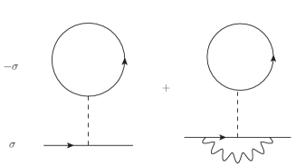
Figure 2: Lowest-order electron self-energy corrections. The second term is that due to the vertex correction. The dashed line indicates the Coulomb interaction $U$ and the wavy line shows the phonon propagator.

We consider the self-energy corrections shown in Fig.2. The first term is the Hartree term that stems from the on-site Coulomb interaction and the second one includes the vertex correction. When we use the approximation in eq.(10), the self-energy is

$$\Sigma_{{\bf k}\sigma}=Un_{-\sigma}+Ug\rho(0)\frac{\omega_{\rm D}}{2\epsilon_{\rm F}}\ln\left(\frac{\epsilon_{\rm F}}{\omega_{\rm D}}\right)n_{-\sigma},$$ (11)

where $g=-\gamma^{2}$ and the number density of electrons with spin $\sigma$ is denoted as $n_{\sigma}=(1/N)\sum_{i}\langle n_{i\sigma}\rangle$ where $N$ is the number of sites.

4.2 Electron susceptibility

We show contributions to the electron susceptibility $\chi^{+-}$ in Fig. 3. They are given by

$$\chi^{(a)}(0)=\sum_{k}G_{0}(k)G_{0}(k)\Gamma(k,k;q=0),$$ (12)

$$\chi^{(b)}(0) = \sum_{k}\sum_{q}G_{0}(k)G_{0}(k+q)G_{0}(k)G_{0}(k+q)$$ (13)

$$\times U\Gamma(k,k+q;q),$$

where $\Sigma_{k}$ indicates $\Sigma_{k}=(1/\beta)\sum_{m}\int d^{d}k/(2\pi)^{d}$. The term in Fig. 3(b) contains the electron-phonon vertex correction as well as the Coulomb interaction. We show the vertex function $\Gamma(k,k+q;q)$ for small $q\simeq 0$ as a function of $\omega_{D}/t$ in Fig.4. We put $k_{0}=0$ and ${\bf k}=(\pi,0,0)$ and ${\bf k}=(\pi/2,\pi/2,\pi/2)$ in three dimensions and ${\bf k}=(\pi,0)$ in two dimensions. The vertex function is of the order of $\omega_{D}/t$ when $\omega_{D}/t$ is small, $\omega_{D}/t\ll 1$, in accordance with the Migdal theorem[34, 36]. The result shows the same behavior regardless of space dimension in two- and three-dimensional cases.

We evaluated $\chi^{(a)}$ and $\chi^{(b)}$ in Fig.3 in two dimensions. We show them in Fig.5 as a function of $\omega_{D}/t$ where the upper line indicates $\chi^{(a)}/g$ and the lower one is for $\chi^{(b)}/Ug$. The result indicates that $\chi^{(b)}/Ug$ is smaller than $\chi^{(a)}/g$ by about two orders of magnitude.

4.3 Two-particle interaction

It was pointed out that the vertex correction to susceptibility $\chi^{+-}$ in Fig.3(b) may give a large contribution to the isotope effect when we include the effective electron-hole two-particle interaction shown in Fig.6[33]. We examine this here. The two-particle interaction in Fig.6 is denoted as $\Pi(p_{1},p_{2};p_{3}.p_{4})$. The susceptibility in Fig.3(b) with the two-particle interaction is written as (Fig.7)

$$\chi^{(b)}_{e-p}(Q) = \sum_{k}\sum_{p}\sum_{q}G(k)G(k+q)G(k+Q)G(k+q+Q)$$ (14)

$$\times (-\gamma^{2})G(p)G(p+q)D(k-p)$$

$$\times \Pi(p,k+Q;p+q,k+q+Q),$$

where $k=(i\epsilon_{m},{\bf k})$, $q=(i\nu_{\ell},{\bf q})$, $p=(i\omega_{n},{\bf p})$ and $Q=(iQ_{0},{\bf Q})$. $G$ and $D$ are Green’s functions including the interaction corrections. For the on-site Coulomb interaction, the effective electron-hole interaction reads

$$\Pi(p_{1},p_{2};p_{3},p_{4})=\frac{U}{1-U\chi(p_{1}-p_{2})},$$ (15)

where $\chi(q)$ is the electron susceptibility. We consider the case $Q=0$. For the ferromagnetic case, $\chi^{(b)}_{e-p}(Q)$ is less than the value obtained by approximating the two-particle interaction $\Pi$ by $U/(1-U\chi(0))$ since $\chi$ may have a peak at $p_{1}-p_{2}=0$. The contribution in Fig. 3(b) is enhanced by the factor $U/(1-U\chi(0))$. When $U$ is near the critical value $U_{c}$, for example, $1-U\chi_{0}\sim-0.1$, the term from $\chi^{(b)}$ is still small compared to that from $\chi^{(a)}$. When $U$ is extremely near $U_{c}$ such as $1-U\chi_{0}\sim-0.01$, the problem becomes delicate. We do not, however, consider this region in this paper because a more precise theory is needed to investigate the critical region.

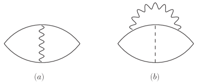
Figure 3: Contributions to the susceptibility $\chi^{+-}$ with the electron-phonon vertex correction. They are denoted as $\chi^{(a)}$ and $\chi^{(b)}$.

Figure 4: Vertex function $\Gamma(k,k+q;q)$ as a function of $\omega_{D}/t$ when $q=(iq_{0},{\bf q})$ is small in the static limit $k_{0}=q_{0}=0$. The wave number ${\bf k}$ is ${\bf k}=(\pi,0,0)$ and ${\bf k}=(\pi/2,\pi/2,\pi/2)$ in three dimensions ($\L\times L\times L$ lattice) and ${\bf k}=(\pi,0)$ in two dimensions ($L\times L$ lattice). The electron dispersion is $\xi_{{\bf k}}=-2t(\cos(k_{x})+\cos(k_{y})+\cos(k_{z}))-\mu$ and $\xi_{{\bf k}}=-2t(\cos(k_{x})+\cos(k_{y}))-\mu$. We put $L=200$ and the summation with respect to the Matsubara frequency is restricted to $-n_{\beta}\leq n\leq n_{\beta}$ with $n_{\beta}=100$ and the inverse temperature $\beta=8/t$. In actual calculations ${\bf q}$ is kept finite such as ${\bf q}=(0.01\pi,0.01\pi,0.01\pi)$.

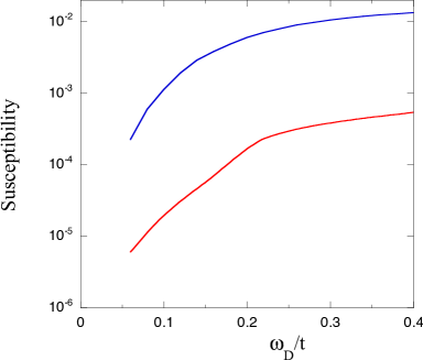
Figure 5: Susceptibilities $\chi^{(a)}/g$ in Fig.3(a) (upper) and $\chi^{(b)}/Ug$ in Fig.3(b) (lower), respectively, as a function of $\omega_{D}/t$.

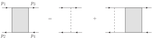
Figure 6: Bethe-Salpeter equation for the effective two-particle electron-hole interaction $\Pi(p_{1},p_{2};p_{3},p_{4})$ with $p_{1}-p_{2}=p_{3}-p_{4}$[36].

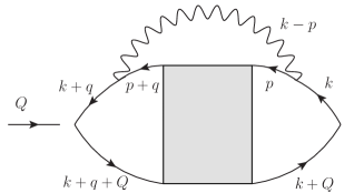
Figure 7: Susceptibility with the effective two-particle interaction and the electron-phonon vertex correction.

5 Isotope effect in itinerant ferromagnets

5.1 Isotope effect in the Stoner theory[33]

The magnetization $\Delta\equiv n_{\uparrow}-n_{\downarrow}$ is determined form the mean-field equation given by

$$n_{\uparrow}-n_{\downarrow}=\frac{1}{V}\sum_{{\bf k}}(f(E_{{\bf k}\uparrow})-f(E_{{\bf k}\downarrow})),$$ (16)

where $E_{{\bf k}\sigma}=\xi_{{\bf k}}+\Sigma_{{\bf k}\sigma}$ and $f(E)$ is the Fermi distribution function. The equation is written as up to the order of $\Delta$:

$$\Delta=-U_{{\rm eff}}\Delta\int d\xi\rho(\xi)f^{\prime}(\xi),$$ (17)

where

$$U_{{\rm eff}}=U+Ug\rho(0)\frac{\omega_{D}}{2\epsilon_{F}}\ln\left(\frac{\epsilon_{F}}{\omega_{D}}\right).$$ (18)

The Curie temperature $T_{\rm c}$ in the mean-field theory is[10]

$$k_{\rm B}T_{\rm c}=\sqrt{A}\sqrt{1-\frac{1}{U_{{\rm eff}}\rho(0)}},$$ (19)

where $A$ is a constant. This result is also obtained from the condition $1/2=U\chi(0)|_{T=T_{c}}$ in the RPA theory. Because the contribution in Fig. 3(b) is small compared with that in Fig. 3(a) (at least except the region just near the critical value of $U$), we neglect the term in Fig. 3(b). Because $\omega_{\rm D}\propto 1/\sqrt{M}$ where $M$ is an corresponding atomic mass, we obtain

$$\frac{\partial\ln T_{\rm c}}{\partial\ln M}=-\frac{1}{4}\frac{1}{U_{{\rm eff}}\rho(0)-1}\frac{\partial\ln U_{{\rm eff}}}{\partial\ln\omega_{\rm D}}.$$ (20)

From this relation, we obtain positive derivative $\partial T_{\rm c}/\partial M>0$. The isotope coefficient $\alpha=-\partial\ln T_{c}/\partial\ln M$ is[33]

$$\alpha=-\frac{1}{4}\frac{U}{U_{\rm eff}(U_{\rm eff}\rho(0)-1)}|g\rho(0)|\frac{\omega_{D}}{2\epsilon_{F}}\Big{[}\ln\left(\frac{\epsilon_{F}}{\omega_{D}}\right)-1\Big{]}.$$ (21)

Let us estimate the shift of $T_{\rm c}$ by using this formula. For $T_{\rm c}=160$K, $M=16$ and $\Delta M=2$, $\Delta T_{\rm c}=-T_{\rm c}\Delta M/M\cdot\alpha$ is

$$\Delta T_{\rm c}\simeq 0.25\frac{1}{U_{\rm eff}\rho(0)-1}|g\rho(0)|,$$ (22)

where the unit is K (kelvin). We obtain $\Delta T_{\rm c}\simeq 0.075$K for $U_{\rm eff}\rho(0)=2$ and $\Delta T_{\rm c}\simeq 0.15$ for $U_{\rm eff}\rho(0)=1.5$ where we set $|g\rho(0)|=0.3$. $U$ should be very close to the critical value of $U$, like $U\rho(0)\sim 1.07$, to agree with the observation $\Delta T_{\rm c}\simeq 1$K.

5.2 Self-consistent spin-fluctuation theory

The physical properties of weak itinerant ferromagnets are well understood by the self-consistent renormalization (SCR) theory of spin fluctuation[10]. We must take account of spin fluctuation to evaluate the isotope shift of $T_{c}$. We use the SCR theory for this purpose. Let us consider the free-energy functional of an $S^{4}$ theory:

$$F = \sum_{\bf q}\left(\frac{1}{2\chi_{0}({\bf q})}-U\right)|{\bf S}_{\bf q}|^{2}+\frac{\lambda}{4}\sum_{j}|{\bf S}_{j}|^{4}-{\bf S}_{{\bf q}=0}\cdot{\bf h}$$ (23)

$$= \sum_{\bf q}\left(\frac{1}{2\chi_{0}({\bf q})}-U\right)|{\bf S}_{\bf q}|^{2}+\frac{\lambda}{4}\frac{1}{N}\sum_{qq^{\prime}q^{\prime\prime}}({\bf S}_{\bf q}\cdot{\bf S}_{-{\bf q}^{\prime}})$$

$$\times ({\bf S}_{{\bf q}^{\prime\prime}}\cdot{\bf S}_{{\bf q}^{\prime}-{\bf q}^{\prime\prime}-{\bf q}})-{\bf S}_{{\bf q}=0}\cdot{\bf h},$$

where ${\bf S}_{j}$ is the spin density and ${\bf h}$ is the magnetic field. $N$ indicates the number of lattice sites. The Fourier decomposition of ${\bf S}_{j}$ is defined by

$${\bf S}_{j}=\frac{1}{\sqrt{N}}\sum_{\bf q}{\bf S}_{\bf q}e^{i{\bf q}\cdot{\bf R}_{j}}.$$ (24)

$\lambda$ is the coupling constant that indicates the strength of the mode-mode couplings, and $\chi_{0}({\bf q})$ is the susceptibility of the non-interacting system. We adopt that ${\bf S}_{{\bf q}=0}=(0,0,S)$ and ${\bf h}=(0,0,h)$ where $S=S(T)$ is the magnetization (order parameter). From the equation $\partial F/\partial S=0$, the susceptibility $\chi(T)\equiv S/h$ is given by

$$\frac{1}{\chi(T)}=\frac{1}{\chi_{0}}-2U+\lambda(3m_{\parallel}^{2}+2m_{\perp}^{2})+\lambda S^{2}.$$ (25)

$\chi_{0}=\chi_{0}({\bf q}=0)$ is the uniform susceptibility and is assumed to be temperature independent: $\chi_{0}=\rho(0)/2$. From the fluctuation-dissipation theorem, $m_{\alpha}^{2}$ is given as

$$m_{\alpha}^{2} = \frac{2}{\pi}\int\frac{d^{3}q}{(2\pi)^{3}}\int_{0}^{\infty}d\omega\left(\frac{1}{2}+\frac{1}{e^{\omega/T}-1}\right){\rm Im}\chi_{\alpha}({\bf q},\omega)$$ (26)

$$= (m_{\alpha}^{2})_{\rm zp}+(m_{\alpha}^{2})_{\rm th}.$$

At $T>T_{\rm c}$ we have $S=0$ so that we can assume $m_{x}^{2}=m_{y}^{2}=m_{z}^{2}$. At $T=T_{\rm c}$ we obtain

$$\frac{1}{\lambda}\left(2U-\frac{1}{\chi_{0}}\right)=5\left(m_{\alpha}^{2}\right)\Big{|}_{T=T_{c}}.$$ (27)

We include the electron-phonon correction in the susceptibility $\chi({\bf q},\omega)$:

$$\chi({\bf q},\omega)=\chi_{el}({\bf q},\omega)+\chi_{e-ph}({\bf q},\omega),$$ (28)

where $\chi_{el}$ is the susceptibility without the electron-phonon correction and $\chi_{e-ph}$ is of order $\omega_{D}/\epsilon_{F}$ coming from the diagram in Fig. 3(a). When we use an approximation in eq.(10), $\chi$ is approximated as

$$\chi({\bf q},\omega)\simeq\chi_{el}({\bf q},\omega)\left(1+g\rho(0)\frac{\omega_{D}}{2\epsilon_{F}}\ln\frac{\epsilon_{F}}{\omega_{D}}\right).$$ (29)

We use the following form for the susceptibility $\chi_{el}({\bf q},\omega)$[10, 40, 41]:

$$\frac{1}{\chi_{el}({\bf q},\omega)}=\frac{1}{\chi_{el}(0,0)}+Aq^{2}-iC\frac{\omega}{q},$$ (30)

where $A$ and $C$ are constants, and $\chi_{el}(0,0)=\chi_{el}(T)$. The electron-phonon interaction gives a correction of order of $\omega_{D}/\epsilon_{F}$. Then at $T=T_{\rm c}$, $(m_{\alpha}^{2})_{\rm th}$ is proportional to $T_{\rm c}^{4/3}(1+c_{0}g\rho(0)\omega_{D}/(2\epsilon_{F})\ln(\epsilon_{F}/\omega_{D}))$ with a constant $c_{0}$. In the approximation in eq.(29), we have $c_{0}=1$. Numerical calculations in Fig. 5 indicate that $c_{0}$ is small, especially for small $\omega_{D}/t$, due to multiple integrals of momenta.

We substitute $U_{\rm eff}$ to $U$ to take account of the electron-phonon interaction. The zero-point fluctuation $(m_{\alpha}^{2})_{\rm zp}$ is simply a constant at $T=T_{\rm c}$ and we include this contribution in $U_{\rm eff}$. This results in a formula for the isotope coefficient $\alpha=-\partial\ln T_{\rm c}/\partial\ln M$ given as

$$\alpha=-\frac{3}{8}\left(\frac{U\rho(0)}{U_{{\rm eff}}\rho(0)-1}-c_{0}\right)|g\rho(0)|\frac{\omega_{\rm D}}{2\epsilon_{\rm F}}\biggl{[}\ln\left(\frac{\epsilon_{\rm F}}{\omega_{\rm D}}\right)-1\biggr{]}.$$ (31)

$\partial\ln T_{c}/\partial\ln M$ is positive when $U_{\rm eff}\rho(0)/(U_{\rm eff}\rho(0)-1)-c_{0}>0$. This inequality holds as far as $c_{0}<1$ for $U_{\rm eff}\rho(0)>1$.

For SrRuO₃, the Debye frequency is $\omega_{D}\simeq 340$cm${}^{-1}\sim 490$K. Then we set $\omega_{D}/\epsilon_{F}\sim 0.05$. For $T_{\rm c}=160{\rm K}$, $M=16$ and $\Delta M=2$, we obtain $\Delta T_{\rm c}=-T_{\rm c}\Delta M/M\cdot\alpha$ as

$$\Delta T_{\rm c}\simeq 0.374\left(\frac{U\rho(0)}{U_{\rm eff}\rho(0)-1}-c_{0}\right)|g\rho(0)|,$$ (32)

in units of K. This formula gives the value which agrees with experimental results. For example, we have $\Delta T_{\rm c}\simeq 0.22$K for $U_{\rm eff}\rho(0)=2$ and $\Delta T_{\rm c}\simeq 0.34$K for $U_{\rm eff}\rho(0)=1.5$, where $g\rho(0)=-0.3$ and we neglect $c_{0}$. $\Delta T_{\rm c}$ increases as $U$ approaches the critical value. The experimental value $\Delta T_{\rm c}\simeq 1$K is obtained when $U\rho(0)\simeq 1.13$.

6 Summary

We have presented a theory of the isotope effect of Curie temperature $T_{c}$ in itinerant ferromagnets. It is primarily important to determine the sign of the shift of $T_{\rm c}$ for isotope substitution. Our picture is that the decrease of the Debye frequency results in the increase of relative strength of the Coulomb interaction and this leads to a positive shift of $T_{\rm c}$ as $M$ increases.

The isotope shift of $T_{\rm c}$ occurs through the electron-phonon coupling. This effect is of order of $\omega_{\rm D}/\epsilon_{\rm F}$ because the electron-phonon interaction is restricted to the region within an energy shell of thickness $\omega_{\rm D}$. We have presented the formula on the basis of the spin-fluctuation theory. The isotope shift of $T_{\rm c}$ is obtained as a function of the electron-phonon coupling $g$ and the on-site Coulomb interaction $U$. These are not determined within a theory, and are treated as parameters. The sign of the isotope shift $\Delta T_{\rm c}$ of the Curie temperature agrees with the experimental result and $\Delta T_{\rm c}$ decreases as $U$ increases. The experimental value of $\Delta T_{\rm c}$ is consistent with the formula if we adopt that $U$ is not far from the critical value of the ferromagnetic transition. This assumption is reasonable for usual itinerant ferromagnetic materials.

Our theory cannot be applied to materials such La_1-xCa_xMnO₃ because the ferromagnetic transition is caused by the double-exchange interaction and the Jahn-Teller effect may play a role in these ferromagnets.

Numerical calculations were performed at the Supercomputer Center of the Institute for Solid State Physics, University of Tokyo.

References

• [1] J. G. Bednorz and K. A. MΓΌller: Z. Phys. B64, 189 (1986).
• [2] The Physics of Superconductor Vol.I and Vol.II, edited by K. H. Bennemann and J. B. Ketterson (Springer, Berlin, 2003).
• [3] P. W. Anderson: The Theory of Superconductivity in the High-Tc Cuprates (Princeton University Press, Princeton, 1997).
• [4] E. Dagotto: Rev. Mod. Phys. 66, 763 (1994).
• [5] G. R. Stewart: Rev. Mod. Phys. 56, 755 (1984).
• [6] H. R. Ott: Prog. Low Temp. Phys. 11, 215 (1987).
• [7] M. B. Maple: Handbook on the Physics and Chemistry of Rare Earths Vol. 30 (North-Holland, Elsevier, Amsterdam, 2000).
• [8] J. Kondo: The Physics of Dilute Magnetic Alloys (Cambridge University Press, Cambridge, 2012).
• [9] T. Ishiguro, K. Yamaji and G. Saito: Organic Superconductors (Springer, Berlin, 1998).
• [10] T. Moriya: Spin Fluctuation in Itinerant Electron Magnetism (Springer, Berlin, 1985).
• [11] J. Hubbard: Proc. Roy. Soc. A276, 238 (1963).
• [12] J. Hubbard: Proc. Roy. Soc. A281, 401 (1964).
• [13] M. C. Gutzwiller: Phys. Rev. Lett. 10, 159 (1963).
• [14] J. Kanamori: Prog. Theor. Phys. 30, 275 (1963).
• [15] T. Yanagisawa and Y. Shimoi: Int. J. Mod. Phys. B10, 3383 (1996).
• [16] K. Yamaji, T. Yanagisawa, T. Nakanishi and S. Koike: Physica C304, 225 (1998).
• [17] T. Yanagisawa: J. Phys. Soc. Jpn. 85, 114707 (2016).
• [18] J. R. Franck, I. Isaac, W. Chen, J. Chrzanowski and J. C. Irwin: J. Phys. Chem. Solids 59, 2199 (1998).
• [19] J. R. Franck, I. Isaac, W. Chen, J. Chrzanowski and J. C. Irwin: Phys. Rev. B58, 5189 (1998).
• [20] L. M. Fisher, A. V. Kalinov and I. F. Voloshin: Phys. Rev. B68, 174403 (2003).
• [21] D. J. Pringle, J. L. Tallon, B. G. Walker and H. J. Trodahl: Phys. Rev. B59, R11679 (1999).
• [22] G. S. Knapp, E. Corenzwit and C. W. Chu: Solid State Commun. 8, 639 (1970)
• [23] H. Kawanaka, Y. Aiura, T. Hasebe, M. Yokoyama, T. Masui, Y. Nishihara and T. Yanagisawa: Sci. Rep. 6, 35150 (2016).
• [24] J. Volger: Physica 20, 49 (1954).
• [25] S. Jin, T. H. Tiefel, M. McCormack, R. A. Fastnacht, R. Ramesh and L. H. Chen: Science 264, 413 (1994)
• [26] C. Zener: Phys. Rev. 82, 403 (1951).
• [27] J. Goodenough: Phys. Rev. 100, 564 (1955).
• [28] P. W. Anderson and H. Hasegawa: Phys. Rev. 100, 675 (1955).
• [29] A. J. Millis, P. B. Littlewood and B. I. Shraiman: Phys. Rev. Lett. 74, 5144 (1995).
• [30] G.-M. Zhao, L. Conder, H. keller and K. A. MΓΌller: Nature 381, 676 (1996).
• [31] G.-M. Zhao, L. Conder, H. keller and K. A. MΓΌller: Phys. Rev. B60, 11914 (1999).
• [32] D. Kirillov, Y. Suzuki, L. Antognazza, K. Char, I. Bozovic and T. H. Geballe: Phys. Rev. B51, 12825 (1995).
• [33] J. Appel and D. Fay: Phys. Rev. B22, 1461 (1980).
• [34] A. A. Abrikosov, L. P. Gor’kov and I. Ye Dzyalosinski: Methods of Quantum Field Theory in Statistical Physics (Dover Publications, New York, 1975).
• [35] A. B. Migdal: Sov. Phys. JETP 7, 996 (1958).
• [36] A. L. Fetter and J. D. Walecka: Quantum Theory of Many-Particle Systems (Dover Publications, New York, 2003).
• [37] J. A. Hertz, K. Levin and M. T. Beal-Monod: Solid State Commun. 18, 803 (1976).
• [38] D. Fay and J. Appel: Phys. Rev. B20, 3705 (1979).
• [39] G. M. Eliashberg: Sov. Phys. JETP 16, 780 (1963).
• [40] J. A. Hertz: Phys. Rev. B14, 1165 (1976).
• [41] A. J. Millis: Phys. Rev. B48, 7183 (1993).