Superconducting-Gravimeter Tests of Local Lorentz Invariance

Abstract

Superconducting-gravimeter measurements are used to test the local Lorentz invariance of the gravitational interaction and of matter-gravity couplings. The best laboratory sensitivities to date are achieved via a maximum-reach analysis for 13 Lorentz-violating operators, with some improvements exceeding an order of magnitude.

Local Lorentz invariance is among the foundational building blocks of General Relativity (GR). Though GR provides an impressive description of the wide variety of gravitational phenomena, standard lore holds that GR may be the low-energy limit of an underlying theory that merges gravitation and quantum physics, such as string theory. Local Lorentz violation may arise in such an underlying framework ks . Hence tests of local Lorentz invariance probe the core construction of GR and may provide clues about the structure of new physics at the quantum-gravity scale. These ideas triggered the development of a comprehensive effective field theory based framework SME ; akgrav for testing Lorentz symmetry used in many modern searches for violations data .

Superconducting gravimeters sens have generated a vast amount of information about the gravitational field of the Earth. Devices functioning at over 2 dozen locations around the globe generate data at minute intervals for the Global Geodynamics Project (GGP) ggp . In some cases measurements span more than a decade, and sensitivities to local variations in the gravitational field approaching parts in $10^{12}$ can be extracted for variations with periods on the order of a day. Stability at the level of parts in $10^{9}$ per year sens has also been achieved. Though the primary use of the data is in geophysical applications, the nature of the data clearly also depends on the foundational theories of physics. Hence these data sets provide opportunities to test fundamental physics shiomi ; gwav . The search for preferred frame effects in gravitational physics, a particular Lorentz-symmetry violating scenario, was perhaps the first application of superconducting gravimeters to tests of foundational theory wg .

In the 4 decades since those early tests, interest in Lorentz violation has surged proc , as have theoretical and experimental developments rev ; revg ; rev2 . In addition to the search for preferred frame effects as a signal of alternatives to GR will , more general types of Lorentz violation are now actively sought as a possible signal of new physics at the Planck scale data . Though performing Planck-scale experiments directly will likely remain infeasible for the foreseeable future, experimental information about the nature of the underlying theory can be attained by searching for tiny Planck-suppressed effects in experiments at presently accessible energies. Lorentz violation provides a useful candidate Planck-suppressed effect ks , and the gravitational Standard-Model Extension (SME) provides a field-theory based framework for organizing a systematic search SME ; akgrav ; nonmin . While sensitivities to SME coefficients for Lorentz violation have been achieved in a variety of gravitational systems hml ; hmd ; gexpt ; llr ; planetary ; pulsar ; akmmgw ; cer , including pioneering work with an atom-interferometer gravimeter hml ; hmd , this work provides the first exploration of superconducting gravimeters in the SME framework and the first search for matter-sector Lorentz violation using gravimeters of any kind. Sensitivity improvements over prior gravimeter work hml ; hmd are achieved for 7 coefficients for Lorentz violation, and the best laboratory sensitivity to 6 coefficients not previously explored in gravimeter experiments is achieved. In some cases, sensitivities are improved by more than a factor of 10.

The SME is constructed as an expansion about the actions of GR and the Standard Model in Lorentz-violating operators of increasing mass dimension. In the present work we focus on the minimal gravitational SME, in which attention is restricted to operators of mass dimension 3 and 4. We consider both the pure-gravity sector lvpn and the spin-independent gravitationally-coupled fermion sector lvgap in the limit of linearized gravity. Though work extending the framework to include higher dimension operators akmmgw ; cer ; ho and nonlinear gravity nlg is now well underway, treatment of these operators lies beyond our present scope. Here we summarize aspects of the SME framework relevant for this work. For additional detail, the reader is referred to Refs. akgrav ; lvpn ; lvgap .

The SME action in this limit can be written $S=S_{G}+S_{\psi}+S^{\prime}$. Here $S_{G}$ is the minimal pure-gravity sector,

$$S_{G}={{1}\over{16\pi G}}\int d^{4}xe(R-uR+s^{\mu\nu}R_{\mu\nu}+t^{\kappa\lambda\mu\nu}C_{\kappa\lambda\mu\nu}),$$ (1)

where $G$ is Newton’s constant, and $R$, $R_{\mu\nu}$, and $C_{\kappa\lambda\mu\nu}$ are the Ricci scalar, Ricci tensor, and Weyl tensor respectively. The symbol $e$ is the determinant of the vierbein $e_{\mu}^{{\phantom{\mu}}a}$, and $u$, $s^{\mu\nu}$, and $t^{\kappa\lambda\mu\nu}$ are coefficient fields having dynamics contained in $S^{\prime}$. Lorentz violating signals in the post-newtonian analysis to follow are associated with $s^{\mu\nu}$, without contribution from $t^{\kappa\lambda\mu\nu}$ yb .

Similarly spin-independent effects in the minimal gravitationally-coupled fermion sector take the form

$$S_{\psi}=\int d^{4}x\left[{\textstyle{1\over 2}}iee^{\mu}_{{\phantom{\mu}}a}\overline{\psi}\Gamma^{a}\stackrel{{\scriptstyle\leftrightarrow}}{{D_{\mu}}}\psi-e\overline{\psi}M\psi\right].$$ (2)

Here $\psi$ is the fermion field and $D_{\mu}$ is the covariant derivative, which, along with the vierbein, provides the coupling to gravity, $\Gamma^{a}\equiv\gamma^{a}-c_{\mu\nu}e^{\nu a}e^{\mu}_{{\phantom{\mu}}b}\gamma^{b}-e_{\mu}e^{\mu a}$, and $M\equiv m+a_{\mu}e^{\mu}_{{\phantom{\mu}}a}\gamma^{a}$. The matter-sector coefficient fields $a_{\mu}$, $e_{\mu}$, and $c_{\mu\nu}$ also have dynamics contained within $S^{\prime}$. The dynamics are assumed to trigger spontaneous Lorentz violation in which the coefficient fields acquire vacuum expectation values, a process for generating Lorentz violation in gravity that is consistent with Riemann geometry akgrav ; rbno . The issue of geometric consistency has also led to the development of SME-based Finsler spacetimes finsler .

Table I. Amplitudes for the force $F_{LV}$.
Amplitude	Phase
$G^{w}_{\omega}=2m^{w}\zeta(\overline{c}{}^{w})_{(XZ)}$
$\phantom{G^{w}_{\omega}=}-{{4}\over{5}}V_{L}\alpha(\overline{a}{}^{w}_{\rm{eff}})_{Y}\sin\chi-2m^{w}V_{L}(\overline{c}{}^{w})_{(TY)}\sin\chi$	$\phi$
$H^{w}_{\omega}=2m^{w}\zeta(\overline{c}{}^{w})_{(YZ)}$
$\phantom{H^{w}_{\omega}=}+{{4}\over{5}}V_{L}\alpha(\overline{a}{}^{w}_{\rm{eff}})_{X}\sin\chi+2m^{w}V_{L}(\overline{c}{}^{w})_{(TX)}\sin\chi$	$\phi$
$G^{w}_{2\omega}=m^{w}\zeta((\overline{c}{}^{w})_{XX}-(\overline{c}{}^{w})_{YY})$	$2\phi$
$H^{w}_{2\omega}=2m^{w}\zeta(\overline{c}{}^{w})_{(XY)}$	$2\phi$
$G^{w}_{\Omega}=2V_{\oplus}\alpha((\overline{a}{}^{w}_{\rm{eff}})_{Y}\cos\eta+(\overline{a}{}^{w}_{\rm{eff}})_{Z}\sin\eta)$
$\phantom{G^{w}_{\Omega}=}+2m^{w}V_{\oplus}\big{[}(\overline{c}{}^{w})_{(TY)}\cos\eta+2(\overline{c}{}^{w})_{(TZ)}\sin\eta\big{]}$	$0$
$H^{w}_{\Omega}=-2V_{\oplus}\alpha(\overline{a}{}^{w}_{\rm{eff}})_{X}-2m^{w}V_{\oplus}(\overline{c}{}^{w})_{(TX)}$	$0$
$E^{\prime w}_{\omega}=-V_{L}\left(2\alpha(\overline{a}{}^{w}_{\rm{eff}})_{Y}+{{4}\over{5}}m^{w}(\overline{c}{}^{w})_{(TY)}\right)\sin\chi$	$\phi$
$F^{\prime w}_{\omega}=V_{L}\left(2\alpha(\overline{a}{}^{w}_{\rm{eff}})_{X}+{{4}\over{5}}m^{w}(\overline{c}{}^{w})_{(TX)}\right)\sin\chi$	$\phi$
$E^{\prime w}_{\Omega}=2V_{\oplus}\alpha((\overline{a}{}^{w}_{\rm{eff}})_{Y}\cos\eta+(\overline{a}{}^{w}_{\rm{eff}})_{Z}\sin\eta)$
$\phantom{E^{w}_{\Omega}=}+2m^{w}V_{\oplus}((\overline{c}{}^{w})_{(TY)}\cos\eta+(\overline{c}{}^{w})_{(TZ)}\sin\eta)$	$0$
$F^{\prime w}_{\Omega}=-2V_{\oplus}\alpha(\overline{a}{}^{w}_{\rm{eff}})_{X}-2m^{w}V_{\oplus}(\overline{c}{}^{w})_{(TX)}$	$0$

The vacuum expectation values, or coefficients for Lorentz violation, are denoted with an overline and, though other choices are possible cl , are typically assumed constant in asymptotically Minkowski spacetimes. For example, the vacuum value associated with the coefficient field $c_{\mu\nu}$ is $\overline{c}{}_{\mu\nu}$ satisfying $\partial_{\alpha}\overline{c}{}_{\mu\nu}=0$. The coefficients parameterize the amount of Lorentz violation in the theory and are the objects sought by experiment. Following generic treatment of spontaneous Lorentz violation and the development of the post-newtonian limit in the pure-gravity sector lvpn and the matter sector lvgap , the signals for Lorentz violation in gravitational experiments can be found. In the work to follow, coefficients for Lorentz violation $\overline{a}{}_{\mu}$ and $\overline{e}{}_{\mu}$ always appear in the combination $(\overline{a}{}_{\rm{eff}})=\overline{a}{}_{\mu}-m\overline{e}{}_{\mu}$. Additionally, $(\overline{a}{}_{\rm{eff}})_{\mu}$ appears with a constant $\alpha$ in gravitational studies, which characterizes coupling constants in the underlying theory. This combination is of special interest since it is typically unobservable in flat spacetime akjt . Note also that the matter-sector coefficients are in general particle-species dependent and a superscript $w$ denotes the associated species. In this work, the focus is on ordinary matter with $w$ referring to proton, neutron, or electron.

The system of interest here can be referred to as a force-comparison gravimeter experiment lvgap . In this class of experiments, the gravitational force on a laboratory body is countered by an appropriate electromagnetic force, and the Lorentz-violating signal can be written

$$F_{LV}=-m^{\rm T}g\sum_{n}\left(A_{n}\cos(\omega_{n}T+\phi_{n})+B_{n}\sin(\omega_{n}T+\phi_{n})\right),$$ (3)

as developed in Sec. VIIC of Ref. lvgap , where

$$A_{n} = \sum_{w}\left({{N^{w}}\over{m^{\rm T}}}G_{n}^{w}+{{N^{w}_{\oplus}}\over{m^{\rm S}}}E_{n}^{\prime w}+{\textstyle{{1}\over{3}}}G_{n}\right),$$

$$B_{n} = \sum_{w}\left({{N^{w}}\over{m^{\rm T}}}H_{n}^{w}+{{N^{w}_{\oplus}}\over{m^{\rm S}}}F_{n}^{\prime w}+{\textstyle{{1}\over{3}}}H_{n}\right).$$ (4)

Here $g$ is the newtonian gravitational field, $m^{\rm T}$ and $m^{\rm S}$ are the conventional Lorentz-invariant mass of the test body and source body respectively, and $N^{w}$ and $N^{w}_{\oplus}$ are the number of particles of type $w$ in the test body and the Earth respectively. Here the test body is a niobium sphere with a mass of a few grams, and the source body is the Earth. The sum over $w$ runs over proton, neutron, and electron. The frequencies $\omega_{n}$ are drawn from the set

$$\omega_{n}\in\{2\omega,\omega,2\omega+\Omega,2\omega-\Omega,\omega+\Omega,\omega-\Omega,\Omega\},$$ (5)

where $\omega$ is the sidereal angular frequency and $\Omega$ is the annual angular frequency. Note that $2\omega$ arises due to the rotation of 2-index coefficients. The corresponding phase $\phi_{n}$ can be obtained from the frequency via the replacement $\omega\rightarrow\phi$, $\Omega\rightarrow 0$, where $\phi$ is a phase that specifies the orientation of the Lab at time $T=0$. The time $T$, along with the spacial coordinates $X,Y,Z$ are the coordinates of the Sun-centered celestial equatorial frame in standard use for SME studies data . The contributions to the Lorentz-violating amplitude $G_{n}^{w}$, $H_{n}^{w}$, $E_{n}^{\prime w}$, and $F_{n}^{\prime w}$ can be found in Table I, while the contributions $G_{n}$ and $H_{n}$ are constructed via Eq. (142) of Ref. lvgap . These are the results developed in lvgap presented here with a few corrections. Here $V_{L}=\omega R$, where $R$ is Earth’s radius and $V_{\oplus}$ is the speed of the Earth on its path around the Sun. The angle $\zeta$ is between the local Lorentz-invariant free-fall direction and the direction of Earth’s center, $\chi$ is the colatitude of the experiment, $\eta$ is the inclination of Earth’s orbit, and $m^{w}$ is the mass of species $w$.

Our method for extracting measurements of the coefficients for Lorentz violation from the GGP data proceeds as follows. We use corrected minute data, which provides a measurement of the gravitational force each minute obtained from the raw data via some repairs performed by the station manager including the removal of some transients such as major earthquakes. Where possible, we follow the methods developed for the atom-interferometer gravimeter analysis hml . The basic idea is to perform a discrete Fourier transform on relevant sets of gravitational force vs. time data to extract the amplitudes $A_{n},B_{n}$. Equation (4) is then used to interpret the amplitudes as measurements of the SME coefficients.

As is typical of SME searches, the amplitudes $A_{n},B_{n}$ extracted from data collected by a particular device at a given site provide a measurement of a linear combination of SME coefficients rather than a measurement of a single term in the underlying theory. The numbers multiplying the coefficients for Lorentz violation in these linear combinations can contain the colatitude of the experiment $\chi$ and dependence on the particle species content of the bodies involved. Hence different sets of data from different locations and/or different devices measure different linear combinations of SME coefficients. Two procedures are common in the literature for extracting sensitivities to individual SME coefficients from such linear combinations. One approach effectively considers a series of special models, each involving one and only one nonzero coefficient for Lorentz violation, hence attributing the measurement of an amplitude $A_{n},B_{n}$ to each of the coefficients it contains individually. This approach is motivated by the thinking that exact cancellation between multiple coefficients in a given measurement is unlikely. We call sensitivities to coefficients for Lorentz violation obtained in this way the “maximum reach” achieved for the given coefficient. The other approach is to treat all coefficients as nonzero simultaneously and use multiple sets of data to separate the linear combinations. We say sensitivities attained in this way are found by “coefficient separation”. In what follows we apply both methods using several sets of gravimeter data.

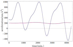
Figure 1: Bad Homburg data taken Jan. 1-3, 2012, before and after tidal model subtraction. Discrete points are plotted that appear as a continuous curve at this scale.

For our maximum-reach analysis we used data from Bad Homburg, Germany, from 2007-2013 (with several gaps of less than 1 week), a site providing some of the cleanest data. Three days of original gravimeter data from Bad Homburg is shown in Fig. 1, appearing as the large-amplitude signal. A daily variation associated with tidal effects is clearly visible in the three peaks. Following Ref. hml we remove the dominate tidal contributions from the signal using a model of solid Earth tides tide . Figure 1 also shows the data after the subtraction of the model. Application of discrete Fourier transform to the residuals,

$$A_{n},B_{n}={\textstyle{{2}\over{K}}}\sum\limits_{k}d(t_{k})\cos,\sin(\omega_{n}t_{k}+\phi),$$ (6)

yields the amplitudes shown in Table II. Here, $K$ is the total number of measurements, $d(t_{k})$ are the residual gravity measurements at times $t_{k}$. Estimated uncertainties are obtained following Refs. hml ; hmd by performing the analysis at several frequencies near the characteristic frequencies and computing the root mean square.

The amplitudes in Table II together with the maximum-reach procedure yield the sensitivities to the coefficients for Lorentz violation shown in the second column of Table III. A dagger $\dagger$ indicates a sensitivity that exceeds previous laboratory tests, though better constraints exist from Solar System or astrophysical observations llr ; planetary ; pulsar ; cer ; bcer . The maximum reach listed here for the $\overline{s}{}^{\mu\nu}$ coefficients, which have previously been explored via gravimeter analysis hml ; hmd , is an improvement upon that work for all 7 coefficients listed.

We perform the same analysis on data collected from the device in Metsahovi, Finland, from 2007-2012, and on a year’s worth of data from Strasbourg, France and from Apache Point, USA taken in 2012. While the maximum reach available from these sites is typically less than that obtained from Bad Homburg, their locations at different colatitudes permit some coefficient separation. We do this following the procedure outlined in Ref. hmd in which each measurement of $A_{n},B_{n}$ provides a probability distribution that we assume to be Gaussian with the measurement and uncertainty providing the center and standard deviation. The probability distribution can then be understood as a function of the coefficients for Lorentz violation through Eq. (4). These probability distributions can then be multiplied together for each of the relevant measurements from each of the 4 sites to obtain an overall probability distribution. Integrating the distribution over all of the coefficients except the one of interest then yields an estimate and uncertainty for that coefficient. The result of this process provides our estimates for the coefficients achieved by coefficient separation shown in the right column of Table III. This procedure for achieving initial coefficient separation estimates assumes the error sources in the 4 experiments are completely independent, while some geophysical noise sources may be somewhat coherent. Though beyond our current scope, it may be possible to address this potential issue through coherent combination of the original data. Relative to Ref. hmd , correlations between amplitudes due to finite data are small and are neglected here.

Table III. Lorentz violation measurements. Coeff. Max reach via 4-site Coeff. Bad Homburg separation $\bar{s}^{XX-YY}$ $2$ $\pm 1\times 10^{-10\dagger}$         - $\bar{s}^{XY}$ $-4$ $\pm 1\times 10^{-10\dagger}$         - $\bar{s}^{XZ}$ $0$ $\pm 1\times 10^{-10\dagger}$ $-2$ $\pm 2\times 10^{-9\dagger}$ $\bar{s}^{YZ}$ $3$ $\pm 1\times 10^{-10\dagger}$ $4$ $\pm 3\times 10^{-9\dagger}$ $\bar{s}^{TX}$ $-3$ $\pm 3\times 10^{-7\dagger}$ $-3$ $\pm 3\times 10^{-7\dagger}$ $\bar{s}^{TY}$ $-6$ $\pm 3\times 10^{-7\dagger}$ $-5$ $\pm 2\times 10^{-7\dagger}$ $\bar{s}^{TZ}$ $-1$ $\pm 1\times 10^{-6\dagger}$ $-1$ $\pm 1\times 10^{-6\dagger}$ $(\bar{c}^{n})_{(TX)}$ $-4$ $\pm 6\times 10^{-6}$ $-3$ $\pm 2\times 10^{-3}$ $(\bar{c}^{n})_{(TY)}$ $-1$ $\pm 1\times 10^{-5}$ $2$ $\pm 4\times 10^{-3}$ $(\bar{c}^{n})_{(TZ)}$ $-1$ $\pm 1\times 10^{-5}$         - $\alpha(\bar{a}^{e+p}_{\rm eff})_{X}$ $-4$ $\pm 6\times 10^{-6}$   GeV^† $3$ $\pm 2\times 10^{-2}$   GeV $\alpha(\bar{a}^{n}_{\rm eff})_{X}$ $-4$ $\pm 5\times 10^{-6}$   GeV^† $-3$ $\pm 2\times 10^{-2}$   GeV $\alpha(\bar{a}^{e+p}_{\rm eff})_{Y}$ $-5$ $\pm 7\times 10^{-6}$   GeV^† $0$ $\pm 4\times 10^{-2}$   GeV $\alpha(\bar{a}^{n}_{\rm eff})_{Y}$ $-4$ $\pm 6\times 10^{-6}$   GeV^† $0$ $\pm 3\times 10^{-2}$   GeV $\alpha(\bar{a}^{e+p}_{\rm eff})_{Z}$ $-1$ $\pm 2\times 10^{-5}$   GeV^†         - $\alpha(\bar{a}^{n}_{\rm eff})_{Z}$ $-1$ $\pm 1\times 10^{-5}$   GeV^†         -

Coefficients $\bar{s}^{XX-YY}$ and $\bar{s}^{XY}$ are obtained from amplitudes in which they are the only coefficient for Lorentz violation involved. Hence these entries in the maximum reach column of Table III could equally be regarded as the results of coefficient separation, and they are omitted from the 4-site analysis. Sufficient information is not available to separate the $\alpha(\bar{a}^{e+p}_{\rm eff})_{Z}$, $\alpha(\bar{a}^{n}_{\rm eff})_{Z}$, and $(\bar{c}^{n})_{TZ}$ coefficients from each other. Hence individual constraints are not available for column 3 of Table III, and the combination is treated as a single coefficient in the separation analysis resulting in $\alpha(\bar{a}^{e+p}_{\rm eff})_{Z}+1.1\alpha(\bar{a}^{n}_{\rm eff})_{Z}+1.1{\rm GeV}\,\,(\bar{c}^{n})_{TZ}=0\pm 6\times 10^{-4}$ GeV. We do not include data from other experiments beyond the 4 gravimeter sites except in excluding from consideration other coefficients that have been constrained much more tightly by nongravitational tests. As this work was completed, the $(\bar{c}^{n})_{TJ}$ were also constrained by nongravitational tests cng . Note that the results of coefficient separation generate improvements over prior lab work for $\overline{s}{}^{\mu\nu}$ coefficients while constraints for matter-sector coefficients are weak. This feature can be traced to the fact that all 4 sites involve niobium test masses and the Earth and hence the same proton/neutron ratios. Note also that proton and electron coefficients are listed together as separating them would require charged matter.

The sensitivities to coefficients in Table III, found via the standard approach to gravimeter analysis in the SME hml ; hmd , provide a basic sense of upper bounds on coefficients. However, some care should be used in interpreting the results. Though we find no compelling evidence of Lorentz violation, some notable deviations from zero are seen in a few cases. In addition to the statistical expectation of a few weak signals when seeking this number of effects, these likely reflect some challenges inherent to the search that we outline here.

The search involves subtracting dominant tidal effects from the gravimeter signal and attributing any remaining periodicity at the characteristic frequencies to Lorentz violation, with uncertainty estimated by the average level of the local Fourier spectrum near the characteristic frequency. The method relies on the assumption that any potential Lorentz-violating signal is not also contained in the tidal model. Modeling of additional local effects is avoided to minimize this concern. We also note that a Fourier transform of the raw data with no tidal modeling yields the same level of reach for annual variations, which is the aspect of the measurement associated with many of the most significant sensitivity improvements. The method also assumes that residual environmental effects at the characteristic frequencies have a size similar to neighboring Fourier amplitudes. This assumption is most challenged by Lorentz-violating frequencies that coincide with dominant tidal components. Here the relatively small residual signal is the result of subtracting a comparatively large modeled tide from a similarly sized signal. One could also imagine the Lorentz-violation signal of a special linear combination of coefficients that matches the tidal phase being masked by a tidal effect.

A variety of opportunities for further improvements with related experiments exist. One key challenge in gravimeter tests is managing periodic environmental effects without using models constructed by fitting to gravimeter data. A way to side-step this issue for matter-sector coefficients is to consider analogous Weak-Equivalence Principle tests that search for variation in the relative gravitational force or acceleration of 2 or more bodies. It may also be possible to use the phase information associated with environmental systematics to separate them from the effects of certain combinations of coefficients for Lorentz violation. Correlations between signals at multiple sites may also be useful. Gravimeter data involving bodies of other compositions would aid in performing coefficient separation for the matter sector. Free-fall gravimeter tests such as atom interferometers are also of interest, particularly for the matter sector, as they involve different dependence on the matter-sector coefficients. An increase in the long-term stability of gravimeters would further improve sensitivities at the annual frequency. Beyond gravimeters, searches for Lorentz violation with satellite geodesy data may be of interest. In all, exciting prospects remain for further searches for Lorentz violation with gravimeters and related systems.

This work was supported in part by the Carleton College Clinton Ford Physics Research Fund.

References

- (1) V.A. Kostelecký and S. Samuel, Phys. Rev. D 39, 683 (1989).
- (2) D. Colladay and V.A. Kostelecký, Phys. Rev. D 55, 6760 (1997); Phys. Rev. D 58, 116002 (1998).
- (3) V.A. Kostelecký, Phys. Rev. D 69, 105009 (2004).
- (4) Data Tables for Lorentz and CPT Violation, V.A. Kostelecký and N. Russell, 2016 edition, arXiv:0801.0287v9.
- (5) J.M. Goodkind, Rev. Sci. Instrum. 70, 4131 (1999).
- (6) The Global Geodynamics Project, http://www.eas.slu.edu/GGP/ggphome.html; J. Hinderer and D. Crossley, J. of Geodynamics 48, 299 (2009).
- (7) S. Shiomi, Prog. Theor. Phys. Supp. 172, 61 (2008).
- (8) M. Coughlin and J. Harms, Phys. Rev. D 90, 042005 (2014).
- (9) K. Nordtvedt and C.M. Will, Astrophys. J. 177, 775 (1972); R.J. Warburton and J.M. Goodkind, Astrophys. J. 208, 881 (1976).
- (10) Proceedings of the Seventh Meeting on CPT and Lorentz Symmetry, V.A. Kostelecký, ed., World Scientific, Singapore, 2017.
- (11) For reviews of the SME approach, see, J.D. Tasson, Rep. Prog. Phys. 77, 062901 (2014); R. Bluhm, Lect. Notes Phys. 702, 191 (2006).
- (12) For a review of the SME gravity sector, see, A. Hees, Q.G. Bailey, A. Bourgoin, H. Pihan-Le Bars, C. Guerlin, and C. Le Poncin-Lafitte, Universe 2, 30 (2016).
- (13) For discussion of other approaches to Lorentz violation see, for example, S. Liberati, Class. Quant. Grav. 30, 133001 (2013), S. Mirshekari, N. Yunes, and C.M. Will, Phys. Rev. D 85, 024041 (2012).
- (14) For a review, see C.M. Will, Theory and Experiment in Gravitational Physics, Cambridge University Press, Cambridge, England, 1993.
- (15) V.A. Kostelecký and M. Mewes, Phys. Rev. D 80, 015020 (2009); Phys. Rev. D 85, 096005 (2012); Phys. Rev. D 88, 096006 (2013).
- (16) H. Müller, S. Chiow, S. Herrmann, S. Chu, K-Y. Chung Phys. Rev. Lett. 100, 031101 (2008).
- (17) K-Y. Chung, S. Chiow, S. Herrmann, S. Chu, and H. Müller, Phys. Rev. D 80, 016002 (2009).
- (18) D. Bennett, V. Skavysh, and J. Long, in V.A. Kostelecký, ed., CPT and Lorentz Symmetry V, World Scientific, Singapore, 2010; J.B.R. Battat, J.F. Chandler, and C.W. Stubbs, Phys. Rev. Lett. 99, 241103 (2007); Q.G. Bailey, R.D. Everett, and J.M. Overduin, Phys. Rev. D 88, 102001 (2013); H. Panjwani, L. Carbone, and C.C. Speake, in V.A. Kostelecký, ed., CPT and Lorentz Symmetry V, World Scientific, Singapore, 2010; J.D. Tasson Phys. Rev. D 86, 124021 (2012); M. Hohensee, H. Müller, and R.B. Wiringa, Phys. Rev. Lett. 111, 151102 (2013); H. Müller et al., Phys. Rev. Lett. 100, 031101 (2008); M. Hohensee et al., Phys. Rev. Lett. 106 151102 (2011). C.-G. Shao et al., Phys. Rev. D 91, 102007 (2015); J. Long and V.A. Kostelecký, Phys. Rev. D 91, 092003 (2015); N. Yunes, K. Yagi, and F. Pretorius, Phys. Rev. D 94, 084002 (2016); M. Schreck, arXiv:1603.07452 C. Le Poncin-Lafitte, A. Hees and S. Lambert, arXiv:1604.01663; A. Bourgoin et al., arXiv:1607.00294; C.-G. Shao et al., Phys. Rev. Lett. 117, 071102 (2016); A. Hees et al., arXiv:1610.04682; J.D. Tasson, Symmetry 8, 111 (2016).
- (19) A. Bourgoin et al., arXiv:1607.00294.
- (20) A. Hees et al., Phys. Rev. D 92, 064049 (2015).
- (21) L. Shao, Phys. Rev. Lett. 112, 111103 (2014); Phys. Rev. D 90, 122009 (2014).
- (22) V.A. Kostelecký and M. Mewes, Phys. Lett. B 757, 510 (2016).
- (23) V.A. Kostelecký and J.D. Tasson, Phys. Lett. B 749, 551 (2015).
- (24) Q.G. Bailey and V.A. Kostelecký, Phys. Rev. D 74, 045001 (2006).
- (25) V.A. Kostelecký, and J.D. Tasson, Phys. Rev. D 83, 016013 (2011).
- (26) V.A. Kostelecký and M. Mewes, arXiv:1611.10313; Q.G. Bailey, V.A. Kostelecký, and R. Xu, Phys. Rev. D 91, 022006 (2015).
- (27) Q.G. Bailey, Phys. Rev. D 94, 065029 (2016); M.D. Seifert, arXiv:1608.01642.
- (28) Y. Bonder, Phys. Rev. D 91, 125002 (2015).
- (29) R. Bluhm, Phys. Rev. D 91, 065034 (2015); Phys. Rev. D 92, 085015 (2015); R. Bluhm and A. Sehic, Phys. Rev. D 94, 104034 (2016).
- (30) V.A. Kostelecký, Phys. Lett. B 701, 137 (2011); V.A. Kostelecký, N. Russell, and R. Tso, Phys. Lett. B 716, 470 (2012); J.E.G. Silva, arXiv:1602.07345; M. Schreck, Phys. Rev. D 94, 025019 (2016); J. Foster and R. Lehnert, Phys. Lett. B 746, 164 (2015); A.B. Aazami and M.A. Javaloyes, Class. Quant. Grav. 33, 025003 (2016); X. Li and S. Wang, Eur. Phys J. C 76, 51 (2016); E. Caponio and G. Stancarone, Int. J. Geom. Meth. Mod. Phys. 13, 1650040 (2016); E. Minguzzi, Rept. Math. Phys. 77, 45 (2016); N. Russell, Phys. Rev. D 91, 045008 (2015); D. Colladay and P. McDonald, Phys. Rev. D 92, 085031 (2015).
- (31) C.D. Lane, Phys. Rev. D 94, 025016 (2016).
- (32) V.A. Kostelecký and J.D. Tasson, Phys. Rev. Lett. 102, 010402 (2009).
- (33) H.-G. Wenzel, ETGTAB3.0 solid earth tide data generation software, http://www.bfo.geophys.uni-stuttgart.de/etgtab.html.
- (34) B. Altschul, Phys. Rev. D 78, 085018 (2008).
- (35) H. Pihan-Le Bars, et al., Phys. Rev. D 95, 075026 (2017).