Leading order relativistic hyperon-nucleon interactions in chiral effective field theory

Abstract

We apply a recently proposed covariant power counting in nucleon-nucleon interactions to study strangeness $S=-1$ $\Lambda N-\Sigma N$ interactions in chiral effective field theory. At leading order, Lorentz invariance introduces 12 low energy constants, in contrast to the heavy baryon approach, where only five appear. The Kadyshevsky equation is adopted to resum the potential in order to account for the non-perturbative nature of hyperon-nucleon interactions. A fit to the $36$ hyperon-nucleon scattering data points yields $\chi^{2}\simeq 16$, which is comparable with the sophisticated phenomenological models and the next-to-leading order heavy baryon approach. However, one cannot achieve a simultaneous description of the nucleon-nucleon phase shifts and strangeness $S=-1$ hyperon-nucleon scattering data at leading order.

3.75.Ev, 12.39.Fe

1 Introduction

Since the quantum number strangeness was introduced [1, 2] and the first observation of $\Lambda$ hypernuclei [3] in 1953, strangeness nuclear physics has always been at the frontier of experimental and theoretical nuclear physics. In recent years, open questions such as charge symmetry breaking in $A=4$ $\Lambda$-hypernuclei [4] and the existence of the H-dibaryon [5] have attracted a lot of attention [6, 7, 8, 9, 10, 11]. In facilities like JLab, J-PARC, KEK, MAMI, and COSY, many important studies are being pursued, e.g., the level spectra and decay properties of $\Lambda$, double $\Lambda$ and $\Xi$ hypernuclei [12, 13, 14, 15, 16], $\Sigma p$ scattering [17], and final state interactions in production reactions, such as $\vec{p}p\rightarrow K^{+}\Lambda p$ [18], which can provide information on the $\Lambda N$ scattering lengths. Meanwhile, theoretical few- and many-body calculations of hypernuclei have made steady progress, see, e.g., Refs. [19, 20]. One particularly interesting ongoing issue is about the role of hyperons in the cores of neutron stars, known as the hyperon puzzle: nuclear many-body calculations incorporating hyperon degrees of freedom [21, 22, 23, 24, 25] have difficulties in obtaining a two-solar mass neutron star that was recently observed [26, 27].

As the most important theoretical input for few- and many-body calculations, baryon-baryon interactions play an indispensable role in studies of hypernuclear physics. Although many efforts have been made to derive them, previous theoretical investigations were mainly based on phenomenological meson-exchange models [28, 29, 30, 31, 32, 33, 34, 35] and quark models [36, 37, 38, 39, 40, 41, 42]. In the past two decades, two breakthroughs have occurred in constructing model-independent baryon-baryon interactions. Both of them are closely related to quantum chromodynamics (QCD), the underlying theory of strong interactions. One breakthrough is lattice QCD simulations [43, 44, 45, 46, 47, 48], which provide an ab initio numerical solution to QCD from first principles. With ever-growing computing power and evolving numerical algorithms, lattice QCD simulations are approaching the physical world [49, 50], thus providing us with more information and constraints on baryon-baryon interactions. The other is chiral effective field theory ($\chi$EFT), which has achieved great successes in nucleon-nucleon ($NN$) interactions [51, 52, 53] following Weinberg’s proposal [54, 55]. The latter approach has been generalized to antinucleon-nucleon [56], hyperon-nucleon ($YN$) [57, 58, 59] and multi-strangeness systems [60, 61, 62]. The main advantage of $\chi$EFT is that by using a power counting scheme, one can improve calculations systematically by going to higher orders in powers of external momenta and light quark masses, and estimating the uncertainties of any given order. Furthermore, three- and four-body forces automatically arise as we push through the hierarchy of chiral forces.

However, the Weinberg approach for baryon-baryon interactions, denoted as the heavy baryon (HB) approach, is based on a non-relativistic formalism. It is sensitive to ultraviolet cutoffs, that is, renormalization group invariance is violated, risking severe model dependence of short-range physics. Various opinions on this issue can be found in Refs. [63, 64, 65, 66, 67, 68, 69, 70]. In two recent papers, Epelbaum and Gegelia have proposed a new approach (referred to as the EG approach in the present paper) to $NN$ scattering in $\chi$EFT [71, 72], where the relativistic effects are partially retained. At leading order (LO), the potential remains unchanged but the scattering equation changes to the Kadyshevsky equation, compared to the Lippmann-Schwinger equation with nonrelativistic nucleon propagators in the HB approach. Although this turned out to describe the Nijmegen partial wave analysis [73] well, a higher order contact term is still needed in the ${}^{3}P_{0}$ partial wave to achieve renormalization group invariance. We applied the EG approach to the strangeness $S=-1$ $YN$ system [74] and found that the best description of the experimental data is quantitatively similar to that of the HB approach, and that cutoff dependence is mitigated but not removed.

Partly motivated by the successes of covariant $\chi$EFT in the one-baryon and heavy-light systems [75, 76, 77, 78, 79, 80, 81, 82, 83], a new covariant power counting is explored in Ref. [84] to study $NN$ chiral interactions. The covariant treatment of baryons maintains all the symmetries and analyticities, and, at LO, it results in a description of the $NN$ phase shifts similar to that of the next-to-leading order (NLO) HB scheme. In the present study, we apply this scheme to $YN$ scattering with strangeness $S=-1$, where more particle channels and less experimental data should be dealt with.

2 Formalism

2.1 Covariant power counting

First, we explain in some detail the covariant power counting scheme proposed in Ref. [84] . Unlike the meson-meson and meson-baryon sectors, such a power counting in the baryon-baryon sector is not yet systematically formulated beyond leading order. In particular, relativistic contact baryon-baryon interactions should be treated carefully, see, e.g. Ref. [85]. In the covariant scheme, one takes the full Dirac spinors for the baryon fields and uses partial derivatives on the baryon/meson fields and meson mass insertions to increase the chiral order.

The perturbative expansion is consistent with conventional $\chi$EFT, in which the scattering amplitude is expanded in terms of a small quantity over a large quantity. The former could be the meson momentum or mass, or the baryon three-momenta, and the latter could be the $\rho$ meson mass or the nucleon mass or the chiral symmetry breaking scale. In Ref. [84], naive dimensional analysis is used to determine the chiral order $\nu$,

$$\nu=2-\frac{1}{2}B+2L+\sum_{i}v_{i}\Delta_{i},~{}~{}~{}~{}~{}~{}\Delta_{i}=d_{i}+\frac{1}{2}b_{i}-2,$$ (1)

where $B$ denotes the number of external baryons, $L$ is the number of Goldstone boson loops and $v_{i}$ is the number of vertices with dimension $\Delta_{i}$. For a vertex with dimension $\Delta_{i}$, $d_{i}$ is the number of derivatives or Goldstone boson masses, and $b_{i}$ is the number of internal baryon lines.

At leading order, there are no derivatives or pseudoscalar meson mass insertions. Therefore, the complete structures are determined by the Clifford algebra ($\Gamma_{i}$), namely the five Lorentz structures shown in the following section. These five structures have been derived in a number of early studies in the nucleon-nucleon sector [57, 86, 85]. Some authors consider the terms involving only $\gamma_{5}$ as higher order because they connect the large and small components of the Dirac spinors [87]. In our present case, we do not expand the Dirac spinors and therefore retain them.

2.2 Leading order baryon-baryon interactions

In covariant power counting [84], the full baryon spinor is retained to maintain Lorentz invariance

$$u_{B}(\mbox{\boldmath$p$},s)=N_{p}\left(\begin{array}[]{c}1\\ \frac{\mbox{\boldmath$\sigma$}\cdot\mbox{\boldmath$p$}}{E_{p}+M_{B}}\end{array}\right)\chi_{s},~{}~{}~{}~{}N_{p}=\sqrt{\frac{E_{p}+M_{B}}{2M_{B}}},$$ (2)

where $E_{p}=\sqrt{\mbox{\boldmath$p$}^{2}+M_{B}^{2}}$, while a non-relativistic reduction of $u_{B}$ is employed in the HB approach. The LO baryon-baryon interactions include non-derivative four-baryon contact terms (CT) and one-pseudoscalar-meson exchange (OPME) potentials, as shown in Fig. 1,

$$V_{\mathrm{LO}}=V_{\mathrm{CT}}+V_{\mathrm{OPME}}.$$ (3)

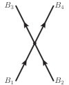
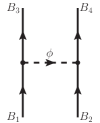
Figure 1: Non-derivative four-baryon contact terms and OPME at LO. The solid lines denote incoming and outgoing baryons ($B_{1,2,3,4}$), and the dashed line denotes the exchanged pseudoscalar meson $\phi$.

2.2.1 Four-baryon contact terms

The Lagrangian term for non-derivative four-baryon contact interactions [57] is

$$\mathcal{L}_{\textrm{CT}}=\sum_{i=1}^{5}\left[\frac{\tilde{C}_{i}^{1}}{2}~{}\textrm{tr}\left(\bar{B}_{1}\bar{B}_{2}(\Gamma_{i}B)_{2}(\Gamma_{i}B)_{1}\right)+\frac{\tilde{C}_{i}^{2}}{2}~{}\textrm{tr}\left(\bar{B}_{1}(\Gamma_{i}B)_{1}\bar{B}_{2}(\Gamma_{i}B)_{2}\right)+\frac{\tilde{C}_{i}^{3}}{2}~{}\textrm{tr}\left(\bar{B}_{1}(\Gamma_{i}B)_{1}\right)\textrm{tr}\left(\bar{B}_{2}(\Gamma_{i}B)_{2}\right)\right],$$ (4)

where $\mathrm{tr}$ indicates the trace in flavor space ($u$, $d$, and $s$). Only baryon fields with the same subscript, 1 or 2, are grouped to form a Lorentz-covariant bilinear. $\Gamma_{i}$ are the elements of the Clifford algebra,

$$\Gamma_{1}=1\,,~{}~{}~{}~{}\Gamma_{2}=\gamma^{\mu}\,,~{}~{}~{}~{}\Gamma_{3}=\sigma^{\mu\nu}\,,~{}~{}~{}~{}\Gamma_{4}=\gamma^{\mu}\gamma_{5}\,,~{}~{}~{}~{}\Gamma_{5}=\gamma_{5}\,;$$ (5)

and $\tilde{C}_{i}^{m}$ ($m=1,2,3$) are the LECs corresponding to independent four-baryon operators. The ground-state octet baryons are collected in the $3\times 3$ traceless matrix:

$$B=\left(\begin{array}[]{ccc}\frac{\Sigma^{0}}{\sqrt{2}}+\frac{\Lambda}{\sqrt{6}}&\Sigma^{+}&p\\ \Sigma^{-}&-\frac{\Sigma^{0}}{\sqrt{2}}+\frac{\Lambda}{\sqrt{6}}&n\\ \Xi^{-}&\Xi^{0}&-\frac{2\Lambda}{\sqrt{6}}\end{array}\right)\,.$$ (6)

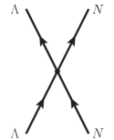
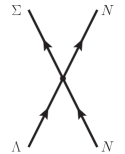
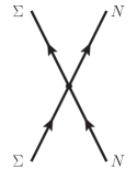
Figure 2: The non-derivative four baryon contact terms in the $\Lambda N-\Sigma N$ system.

The Pauli exclusion principle applies; therefore, the two-baryon wave function is antisymmetric with respect to angular momentum $L$, spin $S$ and flavor. The flavor symmetric and flavor antisymmetric interactions are treated differently by using Fierz rearrangements, as has been done in Ref. [57]. The resulting Lagrangians for strangeness $S=-1$ $YN$ system in the isospin basis are shown in the following, corresponding to the three Feynman diagrams shown in Fig. 2.

$\bullet$  The Lagrangians for the isospin $I=1/2$ $\Lambda N\rightarrow\Lambda N$ reaction are:

$$\mathcal{L}^{\Lambda\Lambda}_{1/2,\textrm{FS}}=\left(\frac{1}{6}C^{1}_{i}+\frac{5}{3}C^{2}_{i}+2C^{3}_{i}\right)\left(\bar{\Lambda}\Gamma_{i}\Lambda\right)\left(\bar{N}\Gamma_{i}N\right)\equiv C^{\Lambda\Lambda}_{i,1/2,\textrm{FS}}\left(\bar{\Lambda}\Gamma_{i}\Lambda\right)\left(\bar{N}\Gamma_{i}N\right),$$ (7)

$$\mathcal{L}^{\Lambda\Lambda}_{1/2,\textrm{FA}}=\left(\frac{3}{2}C^{1}_{i}+C^{2}_{i}+2C^{3}_{i}\right)\left(\bar{\Lambda}\Gamma_{i}\Lambda\right)\left(\bar{N}\Gamma_{i}N\right)\equiv C^{\Lambda\Lambda}_{i,1/2,\textrm{FA}}\left(\bar{\Lambda}\Gamma_{i}\Lambda\right)\left(\bar{N}\Gamma_{i}N\right),$$ (8)

where the subscripts FS and FA are short for flavor symmetric (e.g., ${}^{1}S_{0}$, ${}^{3}P_{0,1,2}\ldots$) and flavor antisymmetric (e.g., ${}^{3}S_{1}$, ${}^{1}P_{1}\ldots$), respectively.

$\bullet$  The Lagrangians for the isospin $I=3/2$ $\Sigma N\rightarrow\Sigma N$ reaction are:

$$\mathcal{L}^{\Sigma\Sigma}_{3/2,\textrm{FS}}=2\left(C^{2}_{i}+C^{3}_{i}\right)\left(\bar{\Sigma}\Gamma_{i}\Sigma\right)\left(\bar{N}\Gamma_{i}N\right)\equiv C^{\Sigma\Sigma}_{i,3/2,\textrm{FS}}\left(\bar{\Sigma}\Gamma_{i}\Sigma\right)\left(\bar{N}\Gamma_{i}N\right),$$ (9)

$$\mathcal{L}^{\Sigma\Sigma}_{3/2,\textrm{FA}}=-2\left(C^{2}_{i}-C^{3}_{i}\right)\left(\bar{\Sigma}\Gamma_{i}\Sigma\right)\left(\bar{N}\Gamma_{i}N\right)\equiv C^{\Sigma\Sigma}_{i,3/2,\textrm{FA}}\left(\bar{\Sigma}\Gamma_{i}\Sigma\right)\left(\bar{N}\Gamma_{i}N\right).$$ (10)

$\bullet$  The Lagrangians for the isospin $I=1/2$ $\Sigma N\rightarrow\Sigma N$ reaction are:

$$\mathcal{L}^{\Sigma\Sigma}_{1/2,\textrm{FS}}=\left(\frac{3}{2}C^{1}_{i}-C^{2}_{i}+2C^{3}_{i}\right)\left(\bar{\Sigma}\Gamma_{i}\Sigma\right)\left(\bar{N}\Gamma_{i}N\right)\equiv C^{\Sigma\Sigma}_{i,1/2,\textrm{FS}}\left(\bar{\Sigma}\Gamma_{i}\Sigma\right)\left(\bar{N}\Gamma_{i}N\right)$$

$$\phantom{\mathcal{L}^{\Sigma\Sigma}_{1/2,\textrm{FS}}}=\left(9C^{\Lambda\Lambda}_{i,1/2,\textrm{FS}}-8C^{\Sigma\Sigma}_{i,1/2,\textrm{FS}}\right)\left(\bar{\Sigma}\Gamma_{i}\Sigma\right)\left(\bar{N}\Gamma_{i}N\right),$$ (11)

$$\mathcal{L}^{\Sigma\Sigma}_{1/2,\textrm{FA}}=\left(\frac{3}{2}C^{1}_{i}+C^{2}_{i}+2C^{3}_{i}\right)\left(\bar{\Sigma}\Gamma_{i}\Sigma\right)\left(\bar{N}\Gamma_{i}N\right)\equiv C^{\Sigma\Sigma}_{i,1/2,\textrm{FA}}\left(\bar{\Sigma}\Gamma_{i}\Sigma\right)\left(\bar{N}\Gamma_{i}N\right)$$

$$\phantom{\mathcal{L}^{\Sigma\Sigma}_{1/2,\textrm{FA}}}=C^{\Lambda\Lambda}_{i,1/2,\textrm{FA}}\left(\bar{\Sigma}\Gamma_{i}\Sigma\right)\left(\bar{N}\Gamma_{i}N\right).$$ (12)

$\bullet$  The Lagrangians for the isospin $I=1/2$ $\Lambda N\rightarrow\Sigma N$ reaction are:

$$\mathcal{L}^{\Lambda\Sigma}_{1/2,\textrm{FS}}=\left(\frac{1}{2}C^{1}_{i}-C^{2}_{i}\right)\left(\bar{\Lambda}\Gamma_{i}\Sigma\right)\left(\bar{N}\Gamma_{i}N\right)\equiv C^{\Lambda\Sigma}_{i,1/2,\textrm{FS}}\left(\bar{\Lambda}\Gamma_{i}\Sigma\right)\left(\bar{N}\Gamma_{i}N\right)$$

$$\phantom{\mathcal{L}^{\Lambda\Sigma}_{1/2,\textrm{FS}}}=3\left(C^{\Lambda\Lambda}_{i,1/2,\textrm{FS}}-C^{\Sigma\Sigma}_{i,1/2,\textrm{FS}}\right)\left(\bar{\Lambda}\Gamma_{i}\Sigma\right)\left(\bar{N}\Gamma_{i}N\right),$$ (13)

$$\mathcal{L}^{\Lambda\Sigma}_{1/2,\textrm{FA}}=-\left(\frac{3}{2}C^{1}_{i}-C^{2}_{i}\right)\left(\bar{\Lambda}\Gamma_{i}\Sigma\right)\left(\bar{N}\Gamma_{i}N\right)\equiv C^{\Lambda\Sigma}_{i,1/2,\textrm{FA}}\left(\bar{\Lambda}\Gamma_{i}\Sigma\right)\left(\bar{N}\Gamma_{i}N\right).$$ (14)

The superscript $YY^{\prime}$ denotes the hyperons in the reaction of $YN\rightarrow Y^{\prime}N$. Strict SU(3) symmetry is imposed, as shown in the second line of Eqs. (11-13). Note that the LECs $C^{1,2,3}_{i}$ here are different from those in Eq. (4) due to the application of Fierz rearrangement [57]. The potentials of the contact terms are derived from Eqs. (7-14), which can be symbolically written as

$$V^{YY^{\prime}}_{\textrm{CT}}=C_{i}^{YY^{\prime}}\left(\bar{u}_{3}\Gamma_{i}u_{1}\right)\left(\bar{u}_{4}\Gamma_{i}u_{2}\right),$$ (15)

where $C_{i}^{YY^{\prime}}$ could be $C^{\Lambda\Lambda}_{i,1/2,\textrm{FS}}$, $C^{\Lambda\Lambda}_{i,1/2,\textrm{FA}}$, $C^{\Sigma\Sigma}_{i,1/2,\textrm{FS}}$, $C^{\Sigma\Sigma}_{i,1/2,\textrm{FA}}$ and $C^{\Lambda\Sigma}_{i,1/2,\textrm{FA}}$. They are first calculated in the helicity basis and then transformed to the $\left|LSJ\right>$ basis [33]. We found that they contribute to all partial waves that have total angular momentum $J\leq 1$ (except for the ${}^{1}P_{1}-^{3}P_{1}$ mixing). We choose the LECs in ${}^{1}S_{0}$, ${}^{3}S_{1}$ and ${}^{3}P_{1}$ to be independent, which is consistent with the $NN$ interactions [84]. The partial wave projected potentials are

$$V^{YY^{\prime}}_{\textrm{CT}}(^{1}S_{0})=\xi_{B}\left[(C_{1}^{YY^{\prime}}+C_{2}^{YY^{\prime}}-6C_{3}^{YY^{\prime}}+3C_{4}^{YY^{\prime}})(1+R_{p}^{2}R_{p^{\prime}}^{2})+(3C_{2}^{YY^{\prime}}+6C_{3}^{YY^{\prime}}+C_{4}^{YY^{\prime}}+C_{5}^{YY^{\prime}})(R_{p}^{2}+R_{p^{\prime}}^{2})\right]$$

$$\phantom{V^{YY^{\prime}}_{\textrm{CT}}(^{1}S_{0})}\equiv\xi_{B}\left[C_{1S0}^{YY^{\prime}}(1+R_{p}^{2}R_{p^{\prime}}^{2})+\hat{C}_{1S0}^{YY^{\prime}}(R_{p}^{2}+R_{p^{\prime}}^{2})\right],$$ (16)

$$V^{YY^{\prime}}_{\textrm{CT}}(^{3}S_{1})=\xi_{B}\left[\frac{1}{9}(C_{1}^{YY^{\prime}}+C_{2}^{YY^{\prime}}+2C_{3}^{YY^{\prime}}-C_{4}^{YY^{\prime}})(9+R_{p}^{2}R_{p^{\prime}}^{2})+\frac{1}{3}(C_{2}^{YY^{\prime}}+2C_{3}^{YY^{\prime}}-C_{4}^{YY^{\prime}}-C_{5}^{YY^{\prime}})(R_{p}^{2}+R_{p^{\prime}}^{2})\right]$$

$$\phantom{V^{YY^{\prime}}_{\textrm{CT}}(^{3}S_{1})}\equiv\xi_{B}\left[\frac{1}{9}C_{3S1}^{YY^{\prime}}(9+R_{p}^{2}R_{p^{\prime}}^{2})+\frac{1}{3}\hat{C}_{3S1}^{YY^{\prime}}(R_{p}^{2}+R_{p^{\prime}}^{2})\right],$$ (17)

$$V^{YY^{\prime}}_{\textrm{CT}}(^{3}P_{1})=\xi_{B}\left[-\frac{4}{3}(C_{1}^{YY^{\prime}}-2C_{2}^{YY^{\prime}}+4C_{3}^{YY^{\prime}}+2C_{4}^{YY^{\prime}}-C_{5}^{YY^{\prime}})R_{p}R_{p^{\prime}}\right]$$

$$\phantom{V^{YY^{\prime}}_{\textrm{CT}}(^{3}P_{1})}\equiv\xi_{B}\left[-\frac{4}{3}C_{3P1}^{YY^{\prime}}R_{p}R_{p^{\prime}}\right],$$ (18)

$$V^{YY^{\prime}}_{\textrm{CT}}(^{3}P_{0})=\xi_{B}\left[-2(C_{1}^{YY^{\prime}}-4C_{2}^{YY^{\prime}}-4C_{4}^{YY^{\prime}}+C_{5}^{YY^{\prime}})R_{p}R_{p^{\prime}}\right]$$

$$\phantom{V^{YY^{\prime}}_{\textrm{CT}}(^{3}P_{0})}=\xi_{B}\left[-2(-C_{1S0}^{YY^{\prime}}-\hat{C}_{1S0}^{YY^{\prime}}+2C_{3S1}^{YY^{\prime}}-2\hat{C}_{3S1}^{YY^{\prime}})R_{p}R_{p^{\prime}}\right],$$ (19)

$$V^{YY^{\prime}}_{\textrm{CT}}(^{1}P_{1})=\xi_{B}\left[-\frac{2}{3}(C_{1}^{YY^{\prime}}+C_{5}^{YY^{\prime}})R_{p}R_{p^{\prime}}\right]$$

$$\phantom{V^{YY^{\prime}}_{\textrm{CT}}(^{1}P_{1})}=\xi_{B}\left[-\frac{2}{3}(C_{3S1}^{YY^{\prime}}-\hat{C}_{3S1}^{YY^{\prime}})R_{p}R_{p^{\prime}}\right],$$ (20)

$$V^{YY^{\prime}}_{\textrm{CT}}(^{3}S_{1}-{}^{3}D_{1})=\xi_{B}\left[\frac{2}{9}\sqrt{2}(C_{1}^{YY^{\prime}}+C_{2}^{YY^{\prime}}+2C_{3}^{YY^{\prime}}-C_{4}^{YY^{\prime}})R_{p}^{2}R_{p^{\prime}}^{2}+\frac{2}{3}\sqrt{2}(C_{2}^{YY^{\prime}}+2C_{3}^{YY^{\prime}}-C_{4}^{YY^{\prime}}-C_{5}^{YY^{\prime}})R_{p}^{2}\right]$$

$$\phantom{V^{YY^{\prime}}_{\textrm{CT}}(^{3}D_{1}-{}^{3}S_{1})}=\xi_{B}\left[\frac{2}{9}\sqrt{2}C_{3S1}^{YY^{\prime}}R_{p}^{2}R_{p^{\prime}}^{2}+\frac{2}{3}\sqrt{2}\hat{C}_{3S1}^{YY^{\prime}}R_{p}^{2}\right],$$ (21)

$$V^{YY^{\prime}}_{\textrm{CT}}(^{3}D_{1}-{}^{3}S_{1})=\xi_{B}\left[\frac{2}{9}\sqrt{2}(C_{1}^{YY^{\prime}}+C_{2}^{YY^{\prime}}+2C_{3}^{YY^{\prime}}-C_{4}^{YY^{\prime}})R_{p}^{2}R_{p^{\prime}}^{2}+\frac{2}{3}\sqrt{2}(C_{2}^{YY^{\prime}}+2C_{3}^{YY^{\prime}}-C_{4}^{YY^{\prime}}-C_{5}^{YY^{\prime}})R_{p^{\prime}}^{2}\right]$$

$$\phantom{V^{YY^{\prime}}_{\textrm{CT}}(^{3}D_{1}-{}^{3}S_{1})}=\xi_{B}\left[\frac{2}{9}\sqrt{2}C_{3S1}^{YY^{\prime}}R_{p}^{2}R_{p^{\prime}}^{2}+\frac{2}{3}\sqrt{2}\hat{C}_{3S1}^{YY^{\prime}}R_{p^{\prime}}^{2}\right],$$ (22)

$$V^{YY^{\prime}}_{\textrm{CT}}(^{3}D_{1})=\xi_{B}\left[\frac{8}{9}(C_{1}^{YY^{\prime}}+C_{2}^{YY^{\prime}}+2C_{3}^{YY^{\prime}}-C_{4}^{YY^{\prime}})R_{p}^{2}R_{p^{\prime}}^{2}\right]$$

$$\phantom{V^{YY^{\prime}}_{\textrm{CT}}(^{3}D_{1})}=\xi_{B}\left[\frac{8}{9}C_{3S1}^{YY^{\prime}}R_{p}^{2}R_{p^{\prime}}^{2}\right],$$ (23)

where $\xi_{B}=N_{p}^{2}N_{p^{\prime}}^{2}$, $R_{p}=|\mbox{\boldmath$p$}|/(E_{p}+M_{B})$, $R_{p^{\prime}}=|\mbox{\boldmath$p$}^{\prime}|/(E_{p^{\prime}}+M_{B})$ and $M_{B}=1080$ MeV stands for the SU(3) average mass of the octet baryons in the chiral limit. $p$ and $p$^′ denote the initial and final momenta, respectively. Note that the second line of Eq. (19) for $V^{YY^{\prime}}_{\textrm{CT}}(^{3}P_{0})$ is only valid for $NN$ interactions, because the structures of the Lagrangians for ${}^{1}S_{0}$ and ${}^{3}S_{1}$ partial waves are different in $\Lambda N-\Sigma N$ systems, as shown in Eqs. (7-14). To recover the potentials in the HB approach we simply take $R_{p}=R_{p^{\prime}}=0$ and $\xi_{B}=1$. The independent potentials respecting SU(3) symmetry are shown in Table 1.

Table 1: Independent contact terms and LECs of strangeness $S=-1$ $YN$ system.

Channel	I	$V$
		${}^{1}S_{0}$	${}^{3}P_{1}$	${}^{3}S_{1}$
$\Lambda N\rightarrow\Lambda N$	$\frac{1}{2}$	$V^{\Lambda\Lambda}_{1S0}$	$V^{\Lambda\Lambda}_{3P1}$	$V^{\Lambda\Lambda}_{3S1}$
$\Lambda N\rightarrow\Sigma N$	$\frac{1}{2}$	$3(V^{\Lambda\Lambda}_{1S0}-V^{\Sigma\Sigma}_{1S0})$	$3(V^{\Lambda\Lambda}_{3P1}-V^{\Sigma\Sigma}_{3P1})$	$V^{\Lambda\Sigma}_{3S1}$
$\Sigma N\rightarrow\Sigma N$	$\frac{1}{2}$	$9V^{\Lambda\Lambda}_{1S0}-8V^{\Sigma\Sigma}_{1S0}$	$9V^{\Lambda\Lambda}_{3P1}-8V^{\Sigma\Sigma}_{3P1}$	$V^{\Lambda\Lambda}_{3S1}$
$\Sigma N\rightarrow\Sigma N$	$\frac{3}{2}$	$V^{\Sigma\Sigma}_{1S0}$	$V^{\Sigma\Sigma}_{3P1}$	$V^{\Sigma\Sigma}_{3S1}$

The analytical form of the potentials, e.g., $V^{\Lambda\Lambda}_{1S0}$, $V^{\Lambda\Lambda}_{1P1}$, can be obtained from Eqs. (16-23). Finally we have 12 independent LECs: $C_{1S0}^{\Lambda\Lambda}$, $\hat{C}_{1S0}^{\Lambda\Lambda}$, $C_{1S0}^{\Sigma\Sigma}$, $\hat{C}_{1S0}^{\Sigma\Sigma}$, $C_{3S1}^{\Lambda\Lambda}$, $\hat{C}_{3S1}^{\Lambda\Lambda}$, $C_{3S1}^{\Sigma\Sigma}$, $\hat{C}_{3S1}^{\Sigma\Sigma}$, $C_{3S1}^{\Lambda\Sigma}$, $\hat{C}_{3S1}^{\Lambda\Sigma}$, $C_{3P1}^{\Lambda\Lambda}$, $C_{3P1}^{\Sigma\Sigma}$. The other three LECs only contribute to the strangeness $S=-2$ system.

2.2.2 One-pseudoscalar-meson-exchange potentials

At LO, we have seven Feynman diagrams for strangeness $S=-1$ systems, as shown in Fig. 3. The OPME potentials are derived from the covariant SU(3) meson-baryon Lagrangian,

$$\mathcal{L}_{MB}^{(1)}=\mathrm{tr}\Bigg{(}\bar{B}\big{(}i\gamma_{\mu}D^{\mu}-M_{B}\big{)}B-\frac{D}{2}\bar{B}\gamma^{\mu}\gamma_{5}\{u_{\mu},B\}-\frac{F}{2}\bar{B}\gamma^{\mu}\gamma_{5}[u_{\mu},B]\Bigg{)}\,,$$ (24)

where $D^{\mu}B=\partial_{\mu}B+[\Gamma_{\mu},B]$ and $D$ and $F$ are the axial vector couplings. In the numerical analysis, we use $D+F=g_{A}=1.277$ [88] and $F/(F+D)=0.4$, where $g_{A}$ is the nucleon axial vector coupling constant. $\Gamma_{\mu}$ and $u_{\mu}$ are the vector and axial vector combinations of the pseudoscalar-meson fields and their derivatives,

$$\Gamma_{\mu}=\frac{1}{2}\left(u^{\dagger}\partial_{\mu}u+u\partial_{\mu}u^{\dagger}\right),\quad u_{\mu}=i(u^{\dagger}\partial_{\mu}u-u\partial_{\mu}u^{\dagger})\,,$$

where $u^{2}=U=\exp\left(i\frac{\sqrt{2}\phi}{f_{0}}\right)$, with the pseudoscalar-meson decay constant $f_{0}\simeq f_{\pi}=92.2$ MeV [88], and the traceless matrix $\phi$ collecting the pseudoscalar-meson fields is:

$$\phi=\left(\begin{array}[]{ccc}\frac{\pi^{0}}{\sqrt{2}}+\frac{\eta}{\sqrt{6}}&\pi^{+}&K^{+}\\ \pi^{-}&-\frac{\pi^{0}}{\sqrt{2}}+\frac{\eta}{\sqrt{6}}&K^{0}\\ K^{-}&\bar{K}^{0}&-\frac{2\eta}{\sqrt{6}}\end{array}\right).$$ (25)

The potentials for OPME can be expressed in a generic form:

$$V_{\mathrm{OPME}}=-N_{B_{1}B_{3}\phi}N_{B_{2}B_{4}\phi}\frac{(\bar{u}_{3}\gamma^{\mu}\gamma_{5}q_{\mu}u_{1})(\bar{u}_{4}\gamma^{\nu}\gamma_{5}q_{\nu}u_{2})}{q^{2}-m^{2}}\mathcal{I}_{B_{1}B_{2}\rightarrow B_{3}B_{4}}\,,$$ (26)

where $q=p^{\prime}-p$ is the momentum transfer, $q^{2}=(E_{p^{\prime}}-E_{p})^{2}-(\mbox{\boldmath$p$}^{\prime}-\mbox{\boldmath$p$})^{2}$, and $m$ is the mass of the exchanged pseudoscalar meson. The SU(3) coefficient $N_{BB^{\prime}\phi}$ and isospin factor $\mathcal{I}_{B_{1}B_{2}\rightarrow B_{3}B_{4}}$ are listed in Refs. [57, 74]. The retardation effects are included in the denominator. Just like the contact terms, Eqs. (15-23), the average baryon mass $M_{B}=1080$ MeV is used in the baryon spinors $u(\bar{u})$ and energies $E_{p(p^{\prime})}$. One can easily obtain $V_{\mathrm{OPME}}$ in the $\left|LSJ\right>$ basis following the same procedure as that for the contact terms. We note that by the mass differences of the exchanged mesons the SU(3) symmetry is broken.

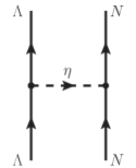
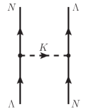
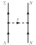
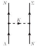
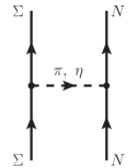
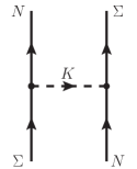
Figure 3: The one-pseudoscalar-meson exchange diagrams in the $\Lambda N-\Sigma N$ system.

In our covariant power counting scheme we keep the complete form of the Dirac spinors and do not perform expansions in terms of small external three momenta, different from what done in the HB approach. In relativistic atomic and nuclear structure studies, the small components of the Dirac spinors have been shown to play an important role, mostly of a dynamical nature. As we will see below, they also play an important role in the present study and result in a good description of $YN$ scattering data. Because the small components are retained, once written in terms of three-momenta and Pauli matrices, the relativistic potential contains terms of higher chiral order in the HB language, similar to the one-baryon sector in covariant chiral perturbation theory. Furthermore, we can see that the LO potentials obtained in the EG approach are the same as those of the HB approach [74], different from the relativistic potentials.

2.3 Scattering equation

The infrared enhancement in two-baryon propagations gives the theoretical argument for low-energy baryon-baryon interactions to be non-perturbative [55]. As a result, one needs to iterate the potentials in the Bethe-Salpeter equation. In practice this is difficult. A three-dimensional reduction of the Bethe-Salpeter equation is often used [89]. In the present work, following Ref. [74], we use the coupled-channel Kadyshevsky equation

$$T_{\rho\rho^{\prime}}^{\nu\nu^{\prime},J}(\mbox{\boldmath$p$}^{\prime},\mbox{\boldmath$p$};\sqrt{s})=V_{\rho\rho^{\prime}}^{\nu\nu^{\prime},J}(\mbox{\boldmath$p$}^{\prime},\mbox{\boldmath$p$})+\sum_{\rho^{\prime\prime},\nu^{\prime\prime}}\int_{0}^{\infty}\frac{dp^{\prime\prime}p^{\prime\prime 2}}{(2\pi)^{3}}\frac{M_{B_{1,\nu^{\prime\prime}}}M_{B_{2,\nu^{\prime\prime}}}~{}V_{\rho\rho^{\prime\prime}}^{\nu\nu^{\prime\prime},J}(\mbox{\boldmath$p$}^{\prime},\mbox{\boldmath$p$}^{\prime\prime})~{}T_{\rho^{\prime\prime}\rho^{\prime}}^{\nu^{\prime\prime}\nu^{\prime},J}(\mbox{\boldmath$p$}^{\prime\prime},\mbox{\boldmath$p$};\sqrt{s})}{E_{1,\nu^{\prime\prime}}E_{2,\nu^{\prime\prime}}\left(\sqrt{s}-E_{1,\nu^{\prime\prime}}-E_{2,\nu^{\prime\prime}}+i\epsilon\right)},$$ (27)

where $\sqrt{s}$ is the total energy of the baryon-baryon system in the center-of-mass frame and $E_{n,\nu^{\prime\prime}}=\sqrt{\mbox{\boldmath$p$}^{\prime\prime}+M_{B_{n,\nu^{\prime\prime}}}}$, $(n=1,2)$. The labels $\nu,\nu^{\prime},\nu^{\prime\prime}$ denote the particle channels, and $\rho,\rho^{\prime},\rho^{\prime\prime}$ denote the partial waves. Relativistic kinematics is used throughout to relate the laboratory momenta to the center-of-mass momenta.

To regularize the integration in the high-momentum region, baryon-baryon potentials are multiplied with an exponential form factor,

$$f_{\Lambda_{F}}(\mbox{\boldmath$p$},\mbox{\boldmath$p$}^{\prime})=\exp\left[-\left(\frac{\mbox{\boldmath$p$}}{\Lambda_{F}}\right)^{2n}-\left(\frac{\mbox{\boldmath$p$}^{\prime}}{\Lambda_{F}}\right)^{2n}\right]\,,$$ (28)

where $n=2$ [90]. Note that Eq. (28) is not a covariant cutoff function. Although there exist covariant cutoff functions of $q^{2}$, they are not favored in constructing chiral forces because they will introduce additional angular dependence to partial wave potentials and thus affect the interpretation of contact interactions. It would be interesting to construct a separable and covariant cutoff function and study its consequences in the future.

The Kadyshevsky equation is solved in the particle basis in order to properly account for the physical thresholds and the Coulomb force in charged channels. The latter is treated with the Vincent-Phatak method [91].

3 Fitting procedure

In our approach, there are 12 LECs that need to be pinned down by fitting to the 36 $YN$ scattering data points as done in Ref. [74], which consist of 35 cross sections [92, 93, 94, 95] and a $\Sigma^{-}p$ inelastic capture ratio at rest [98].

Due to the poor quality of experimental data, it is customary to consider the hypertriton ${}^{3}_{\Lambda}$H binding energy [99, 100] as a further constraint, which is crucial in fixing the relative strength of the ${}^{1}S_{0}$ and ${}^{3}S_{1}$ contributions to $\Lambda p$ scattering. However, we are unable to perform a 3-body calculation at present, so we use as benchmarks the $\Lambda p$ $S$-wave scattering lengths extracted in the LO [57] and next-to-leading order (NLO) [59] HB calculations, mainly because they combine to describe the hypertriton very well [101]. In addition, it seems necessary that $a^{\Lambda p}_{1S0}$ should be neither smaller nor too much larger than $a^{\Lambda p}_{3S1}$, as shown in Ref. [102].

Another constraint that should be considered is the $\Sigma^{+}p$ ${}^{3}S_{1}$ scattering length. A repulsive $\Sigma N$ interaction with isospin $I=3/2$ is obtained from recent experiments [103, 104, 105, 106, 107, 108, 109]. In addition, the conventional $G$-matrix calculations [110] indicate that the ${}^{3}S_{1}$ partial wave for $I=3/2$ $\Sigma N$ should be at least moderately repulsive, therefore in our fits we require a positive $a^{\Sigma^{+}p}_{3S1}$.

Previous works in $\chi$EFT [57, 59, 74] showed that the optimum cutoff $\Lambda_{F}$ may be around 600 MeV. Therefore we first tentatively fix $\Lambda_{F}$ at $600$ MeV. With this cutoff we find that the best description of the experimental data yields $a^{\Lambda p}_{3S1}\approx-1.30\pm 0.02$ fm and $a^{\Lambda p}_{1S0}\approx-2.44^{+0.16}_{-0.54}$ fm. These numbers are between the LO and NLO HB results, which are $a^{\Lambda p}_{3S1}=-1.23$ fm (LO), $a^{\Lambda p}_{3S1}=-1.54$ fm (NLO), $a^{\Lambda p}_{1S0}=-1.91$ fm (LO), and $a^{\Lambda P}_{1S0}=-2.91$ fm (NLO). Best fits within $\Lambda_{F}=500-850$ MeV yield similar scattering lengths. In the results presented below, we fix $a^{\Lambda p}_{3S1}=-1.32$ fm and $a^{\Lambda p}_{1S0}=-2.44$ fm. It should be noted that at present we could in principle choose other combinations within the uncertainties allowed in the best fits. To fix them uniquely, more experimental inputs are needed .

We have made an attempt at a combined fit to the $NN$ and $YN$ data, in which strict SU(3) symmetry was imposed upon the contact terms so that no additional LECs are needed. However, we failed to describe the $NN$ and $YN$ data simultaneously. As a result, consistent with previous NLO results in the HB approach [59], we conclude that one needs to treat SU(3) symmetry breaking more carefully in order to simultaneously describe both the $NN$ and the $YN$ systems in $\chi$EFT.

4 Results and discussion

With the three additional constraints $a^{\Lambda p}_{1S0}=-2.44$ fm, $a^{\Lambda p}_{3S1}=-1.32$ fm and $a^{\Sigma^{+}p}_{3S1}>0$ as explained above, we perform a fit to the 36 scattering data points while varying the cutoff $\Lambda_{F}$. The dependence of $\chi^{2}$ on the cutoff is shown in Fig. 4, in comparison with other approaches. One can see that our new covariant $\chi$EFT approach shows a clear improvement in describing the $YN$ data compared with the HB and EG approach at LO, and the cutoff dependence is much mitigated, both of which are comparable with the NLO HB approach [59].

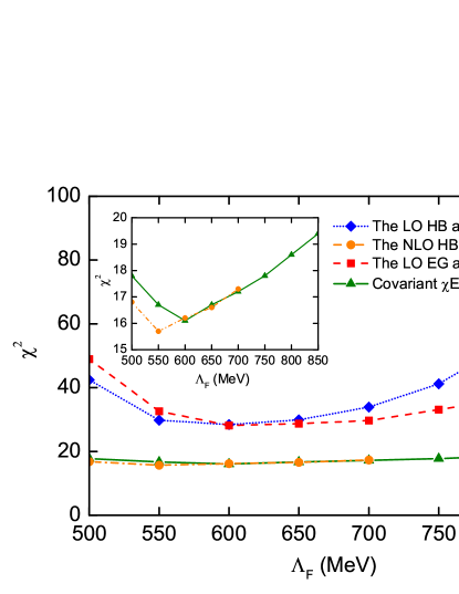
Figure 4: $\chi^{2}$ as a function of the cutoff in the covariant $\chi$EFT approach at LO (green solid line), the HB approach at LO (blue dotted line), NLO (orange dashed-dotted line) [59] and the EG approach at LO (red dashed line).

The minimum value of the $\chi^{2}$ is about 16.1, located at $\Lambda_{F}=550-650$ MeV. Note that the NSC97a-f [30] models, which provide the best description among the phenomenological potentials of the 36 scattering data points, also have a $\chi^{2}$ around 16.

The best fitted LECs obtained with $\Lambda_{F}=600$ MeV are listed in Table 2. Since the LECs in the $\Lambda p$ ${}^{1}S_{0}$ partial wave cannot be uniquely determined, as mentioned previously, we only show a typical case here. One should note that these LECs are certain combinations of those appearing in the Lagrangians, and hence they are not necessarily of the same order of magnitude (see, e.g., Refs. [57, 59]).

In Fig. 5 we compare the descriptions of the experimental cross sections that we have used in the fitting procedure with the LO HB approach. The NSC97f [30] and Jülich 04 results [35] are also shown for comparison. It is clear that the covariant $\chi$EFT approach can reproduce the experimental data rather well. The cusp at the $\Sigma N$ threshold in the $\Lambda p\rightarrow\Lambda p$ reaction is also reproduced well. Note that the experimental data with $P_{\textrm{lab}}>300$ MeV are not used in the fitting procedure.

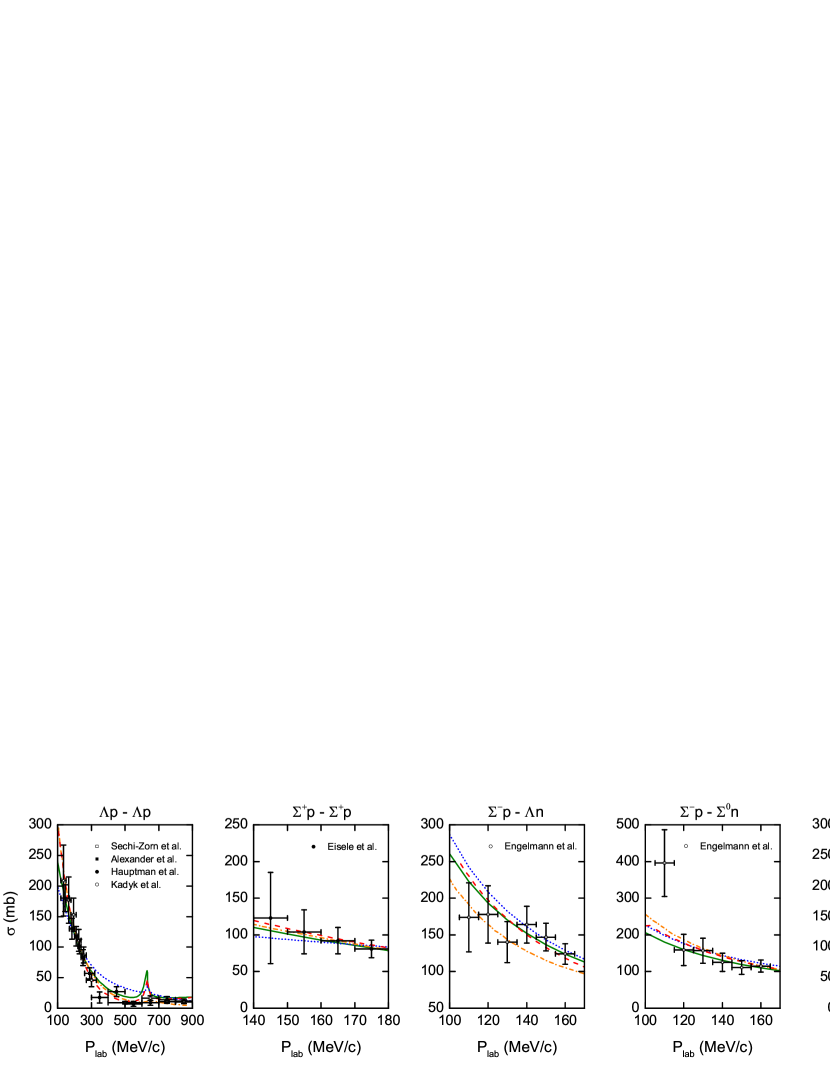
Figure 5: Cross sections in the covariant $\chi$EFT approach (green solid lines) and HB approach (blue dotted lines) at LO as functions of the laboratory momentum at $\Lambda_{F}=600$ MeV. For reference, the NSC97f [30] (red dashed lines) and Jülich 04 [35] (orange dashed-dotted lines) results are also shown. The experimental data are taken from Sechi-Zorn et al. [92], Alexander et al. [93], Eisele et al. [94], Engelmann et al. [95], Hauptman et al. [96] and Kadyk et al. [97].

Table 2: Low-energy constants (in units of $10^{4}$ GeV^-2) at $\Lambda_{F}=600$ MeV in the covariant $\chi$EFT approach.

LECs	$C^{\Lambda\Lambda}_{1S0}$	$C^{\Sigma\Sigma}_{1S0}$	$C^{\Lambda\Lambda}_{3S1}$	$C^{\Sigma\Sigma}_{3S1}$	$C^{\Lambda\Sigma}_{3S1}$	$\hat{C}^{\Lambda\Lambda}_{1S0}$	$\hat{C}^{\Sigma\Sigma}_{1S0}$	$\hat{C}^{\Lambda\Lambda}_{3S1}$	$\hat{C}^{\Sigma\Sigma}_{3S1}$	$\hat{C}^{\Lambda\Sigma}_{3S1}$	$C^{\Lambda\Lambda}_{3P1}$	$C^{\Sigma\Sigma}_{3P1}$
	$-0.0096$	$-0.0276$	$0.0110$	$0.0872$	$0.0257$	$4.2463$	$4.6182$	$0.3660$	$-0.4132$	$0.8499$	$0.2044$	$0.2616$

Due to the lack of near-threshold experimental data, the value of the $\Lambda p\rightarrow\Lambda p$ cross section at rest is not yet known. Our value is about 350 mb, which is smaller than the two phenomenological models. Our result in the $\Sigma^{-}p\rightarrow\Lambda n$ reaction is similar to the LO HB approach and NSC97f results, but quite different from the Jülich 04 model. This channel can partially reflect the nature of $\Lambda N-\Sigma N$ coupling, which is crucial in hypernuclear structure calculations [19]. It is interesting to note that the Jülich 04 model predicts an overbound $\Lambda$ single particle potential $U_{\Lambda}(0)$ in $G$-matrix calculations. On the other hand, the results from the former two are much closer to the empirical value, c.f. Ref. [110] and references therein. In addition, the differential cross sections shown in Fig. 6 are also well predicted within experimental uncertainties, although those data are not taken into account in the fitting procedure.

$S$- and $P$-wave phase shifts of $\Lambda p$ and $\Sigma^{+}p$ reactions are shown in Figs. 7-8. The ${}^{1}S_{0}$ and ${}^{3}P_{0}$ phase shifts are quite different from those of the LO HB approach, but the ${}^{3}P_{2}$ phase shifts are similar, where only OPME terms contribute. Furthermore, the ${}^{1}S_{0}$ phase shifts are similar to those of the NLO HB approach [59].

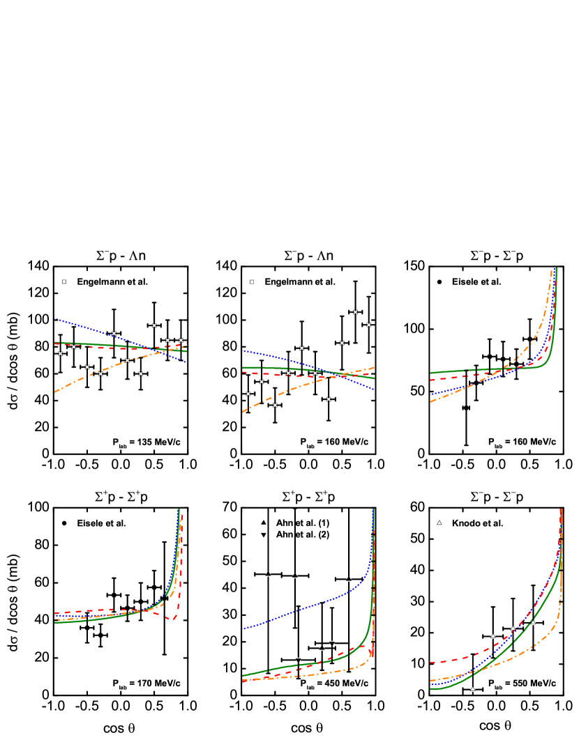
Figure 6: Differential cross sections as a function of cos$\theta$ at various laboratory momenta $P_{\textrm{lab}}$, where $\theta$ is the center-of-mass scattering angle. The covariant $\chi$EFT approach is shown by the green solid lines, the HB approach at LO by the blue dotted lines, the NSC97f [30] results by the red dashed lines, and the Jülich 04 [35] results by the orange dashed-dotted lines. The experimental data are taken from Engelmann et al. [95], Eisele et al. [94], Ahn et al. [111, 112] and Kohno et al. [113].

The improved description of the scattering data by the covariant $\chi$EFT scheme for the most part arises from the contact terms. In the LO HB approach, contact terms only appear in central and spin-spin potentials without momentum dependence, which only contribute to the ${}^{1}S_{0}$ and ${}^{3}S_{1}$ partial waves. In covariant power counting, tensor, spin-orbit and quadratic spin-orbit terms appear at LO in addition to the central and spin-spin terms, namely the momentum dependent terms of $R_{p~{}(p^{\prime})}^{2}$ in Eqs. (16-23). These terms are responsible for the improved description. On the other hand, relativistic corrections to the OPME terms are small. As a result, phase shifts of higher partial waves where only such terms contribute are similar in the covariant and HB approaches at LO. A related discussion for the $NN$ sector can be found in Ref. [84].

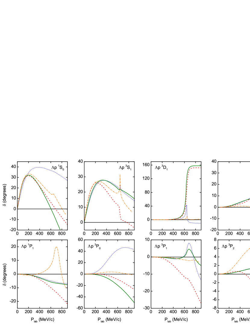
Figure 7: $\Lambda p$ $S$- and $P$-wave phase shifts in the covariant $\chi$EFT approach (green solid lines) and HB approach (blue dotted lines) at LO as functions of the laboratory momentum at $\Lambda_{F}=600$ MeV. For reference, the NSC97f [30] (red dashed lines) and Jülich 04 [35] (orange dashed-dotted lines) results are also shown.

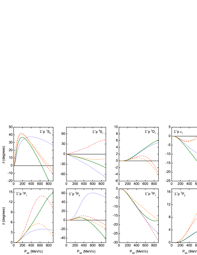
Figure 8: $\Sigma^{+}p$ $S$- and $P$-wave phase shifts in the covariant $\chi$EFT approach (green solid lines) and HB approach (blue dotted lines) at LO as functions of the laboratory momentum at $\Lambda_{F}=600$ MeV. For reference, the NSC97f [30] (red dashed lines) and Jülich 04 [35] (orange dashed-dotted lines) results are also shown.

5 Summary and outlook

We have studied strangeness $S=-1$ hyperon-nucleon scattering at leading order in a covariant framework of chiral effective field theory. Starting from the covariant chiral Lagrangian, the small components of the baryon spinors are retained in deriving the potentials in order to preserve Lorentz invariance. Strict SU(3) symmetry is imposed on the contact terms, which yield 12 independent low energy constants. SU(3) symmetry is broken in the one-pseudoscalar-meson-exchange potentials because of the mass difference of exchanged mesons. The potentials are iterated using the Kadyshevsky equation. A quite satisfactory description of the 36 hyperon-nucleon scattering data points is obtained and the cutoff dependence is shown to be mitigated, both of which are comparable with the next-to-leading order heavy baryon approach. However, one cannot achieve a simultaneous description of the nucleon-nucleon phase shifts and strangeness $S=-1$ hyperon-nucleon scattering data at leading order. The relativistic interactions obtained in the this work may provide essential inputs to relativistic hypernuclear structure studies, e.g., relativistic Brueckner-Hartree-Fork theory in many-body systems.

References

- [1] M. Gell-Mann, Phys. Rev. 92, 833 (1953).
- [2] T. Nakano and K. Nishijima, Prog. Theor. Phys. 10, 581 (1953).
- [3] M. Danysz, and J. Pniewski, Philos. Mag. Ser. 5 44, 348 (1953).
- [4] M. Bedjidian et al. [CERN-Lyon-Warsaw Collaboration], Phys. Lett. 83B, 252 (1979).
- [5] R. L. Jaffe, Phys. Rev. Lett. 38, 195 (1977) Erratum: [Phys. Rev. Lett. 38, 617 (1977)].
- [6] A. Nogga, H. Kamada and W. Glöckle, Phys. Rev. Lett. 88, 172501 (2002) [nucl-th/0112060].
- [7] D. Gazda and A. Gal, Phys. Rev. Lett. 116, 122501 (2016) [arXiv:1512.01049 [nucl-th]].
- [8] S. R. Beane et al. [NPLQCD Collaboration], Phys. Rev. Lett. 106, 162001 (2011) [arXiv:1012.3812 [hep-lat]].
- [9] T. Inoue et al. [HAL QCD Collaboration], Phys. Rev. Lett. 106, 162002 (2011) [arXiv:1012.5928 [hep-lat]].
- [10] J. Haidenbauer and U. -G. Meißner, Phys. Lett. B 706, 100 (2011) [arXiv:1109.3590 [hep-ph]].
- [11] Y. Yamaguchi and T. Hyodo, Phys. Rev. C 94, 065207 (2016) [arXiv:1607.04053 [hep-ph]].
- [12] T. Gogami et al., Phys. Rev. C 93, 034314 (2016) [arXiv:1511.04801 [nucl-ex]].
- [13] A. Esser et al. [A1 Collaboration], Phys. Rev. Lett. 114, 232501 (2015) [arXiv:1501.06823 [nucl-ex]].
- [14] T. O. Yamamoto et al. [J-PARC E13 Collaboration], Phys. Rev. Lett. 115, 222501 (2015) [arXiv:1508.00376 [nucl-ex]].
- [15] J. K. Ahn et al. [E373 (KEK-PS) Collaboration], Phys. Rev. C 88, 014003 (2013).
- [16] K. Nakazawa et al., PTEP 2015, 033D02 (2015).
- [17] See list of proposals at http://j-parc.jp/researcher/Hadron/en /Proposal_e.html.
- [18] F. Hauenstein et al. [COSY-TOF Collaboration], arXiv:1607.04783 [nucl-ex].
- [19] E. Hiyama, S. Ohnishi, B. F. Gibson and T. A. Rijken, Phys. Rev. C 89, 061302 (2014) [arXiv:1405.2365 [nucl-th]].
- [20] X. R. Zhou, H.-J. Schulze, H. Sagawa, C. X. Wu and E. G. Zhao, Phys. Rev. C 76, 034312 (2007).
- [21] E. Massot, J. Margueron and G. Chanfray, Europhys. Lett. 97, 39002 (2012) [arXiv:1201.2772 [nucl-th]].
- [22] H.-J. Schulze and T. Rijken, Phys. Rev. C 84, 035801 (2011).
- [23] J. N. Hu, A. Li, H. Toki and W. Zuo, Phys. Rev. C 89, 025802 (2014) [arXiv:1307.4154 [nucl-th]].
- [24] T. Miyatsu, S. Yamamuro and K. Nakazato, Astrophys. J. 777, 4 (2013) [arXiv:1308.6121 [astro-ph.HE]].
- [25] R. Mallick, Phys. Rev. C 87, 025804 (2013) [arXiv:1207.4872 [astro-ph.HE]].
- [26] P. Demorest, T. Pennucci, S. Ransom, M. Roberts and J. Hessels, Nature 467, 1081 (2010) [arXiv:1010.5788 [astro-ph.HE]].
- [27] J. Antoniadis et al., Science 340, 6131 (2013) [arXiv:1304.6875 [astro-ph.HE]].
- [28] M. M. Nagels, T. A. Rijken and J. J. de Swart, Phys. Rev. D 15, 2547 (1977).
- [29] P. M. M. Maessen, T. A. Rijken and J. J. de Swart, Phys. Rev. C 40, 2226 (1989).
- [30] T. A. Rijken, V. G. J. Stoks and Y. Yamamoto, Phys. Rev. C 59, 21 (1999) [nucl-th/9807082].
- [31] T. A. Rijken and Y. Yamamoto, Phys. Rev. C 73, 044008 (2006) [nucl-th/0603042].
- [32] M. M. Nagels, T. A. Rijken and Y. Yamamoto, arXiv:1501.06636 [nucl-th].
- [33] B. Holzenkamp, K. Holinde and J. Speth, Nucl. Phys. A 500, 485 (1989).
- [34] A. Reuber, K. Holinde and J. Speth, Nucl. Phys. A 570, 543 (1994).
- [35] J. Haidenbauer and U. -G. Meißner, Phys. Rev. C 72, 044005 (2005) [nucl-th/0506019].
- [36] U. Straub, Z. Y. Zhang, K. Brauer, A. Faessler, S. B. Khadkikar and G. Lubeck, Nucl. Phys. A 483, 686 (1988).
- [37] U. Straub, Z. Y. Zhang, K. Braeuer, A. Faessler, S. B. Khadkikar and G. Luebeck, Nucl. Phys. A 508, 385C (1990).
- [38] Z. Y. Zhang, A. Faessler, U. Straub and L. Y. Glozman, Nucl. Phys. A 578, 573 (1994).
- [39] Z. Y. Zhang, Y. W. Yu, P. N. Shen, L. R. Dai, A. Faessler and U. Straub, Nucl. Phys. A 625, 59 (1997).
- [40] J. L. Ping, F. Wang and J. T. Goldman, Nucl. Phys. A 657, 95 (1999) [nucl-th/9812068].
- [41] Y. Fujiwara, C. Nakamoto and Y. Suzuki, Phys. Rev. Lett. 76, 2242 (1996).
- [42] Y. Fujiwara, Y. Suzuki and C. Nakamoto, Prog. Part. Nucl. Phys. 58, 439 (2007) [nucl-th/0607013].
- [43] S. R. Beane et al. [NPLQCD Collaboration], Nucl. Phys. A 794, 62 (2007) [hep-lat/0612026].
- [44] H. Nemura, N. Ishii, S. Aoki and T. Hatsuda, Phys. Lett. B 673, 136 (2009) [arXiv:0806.1094 [nucl-th]].
- [45] S. R. Beane et al. [NPLQCD Collaboration], Phys. Rev. D 81, 054505 (2010) [arXiv:0912.4243 [hep-lat]].
- [46] T. Inoue et al. [HAL QCD Collaboration], Prog. Theor. Phys. 124, 591 (2010) [arXiv:1007.3559 [hep-lat]].
- [47] S. R. Beane et al. [NPLQCD Collaboration], Phys. Rev. D 85, 054511 (2012) [arXiv:1109.2889 [hep-lat]].
- [48] K. Sasaki et al. [HAL QCD Collaboration], PTEP 2015, 113B01 (2015) [arXiv:1504.01717 [hep-lat]].
- [49] T. Doi et al., arXiv:1512.01610 [hep-lat].
- [50] T. Doi et al., arXiv:1512.04199 [hep-lat].
- [51] P. F. Bedaque and U. van Kolck, Ann. Rev. Nucl. Part. Sci. 52, 339 (2002) [nucl-th/0203055].
- [52] E. Epelbaum, H. W. Hammer and U. -G. Meißner, Rev. Mod. Phys. 81, 1773 (2009) [arXiv:0811.1338 [nucl-th]].
- [53] R. Machleidt and D. R. Entem, Phys. Rept. 503, 1 (2011) [arXiv:1105.2919 [nucl-th]].
- [54] S. Weinberg, Phys. Lett. B 251, 288 (1990).
- [55] S. Weinberg, Nucl. Phys. B 363, 3 (1991).
- [56] X. W. Kang, J. Haidenbauer and U. -G. Meißner, JHEP 1402, 113 (2014) [arXiv:1311.1658 [hep-ph]].
- [57] H. Polinder, J. Haidenbauer and U. -G. Meißner, Nucl. Phys. A 779, 244 (2006) [nucl-th/0605050].
- [58] J. Haidenbauer, U. -G. Meißner, A. Nogga and H. Polinder, Lect. Notes Phys. 724, 113 (2007) [nucl-th/0702015 [NUCL-TH]].
- [59] J. Haidenbauer, S. Petschauer, N. Kaiser, U.-G. Meißner, A. Nogga and W. Weise, Nucl. Phys. A 915, 24 (2013) [arXiv:1304.5339 [nucl-th]].
- [60] H. Polinder, J. Haidenbauer and U.-G. Meißner, Phys. Lett. B 653, 29 (2007) [arXiv:0705.3753 [nucl-th]].
- [61] J. Haidenbauer and U.-G. Meißner, Phys. Lett. B 684, 275 (2010) [arXiv:0907.1395 [nucl-th]].
- [62] J. Haidenbauer, U.-G. Meißner and S. Petschauer, Nucl. Phys. A 954, 273 (2016) [arXiv:1511.05859 [nucl-th]].
- [63] G. P. Lepage, nucl-th/9706029.
- [64] M. C. Birse, Phys. Rev. C 74, 014003 (2006) [nucl-th/0507077].
- [65] A. Nogga, R. G. E. Timmermans and U. van Kolck, Phys. Rev. C 72, 054006 (2005) [nucl-th/0506005].
- [66] E. Epelbaum and U.-G. Meißner, Few Body Syst. 54, 2175 (2013) [nucl-th/0609037].
- [67] B. Long and U. van Kolck, Annals Phys. 323, 1304 (2008) [arXiv:0707.4325 [quant-ph]].
- [68] C.-J. Yang, C. Elster and D. R. Phillips, Phys. Rev. C 80, 044002 (2009) [arXiv:0905.4943 [nucl-th]].
- [69] M. P. Valderrama, Phys. Rev. C 83, 024003 (2011) [arXiv:0912.0699 [nucl-th]].
- [70] B. Long and C. J. Yang, Phys. Rev. C 85, 034002 (2012) [arXiv:1111.3993 [nucl-th]].
- [71] E. Epelbaum and J. Gegelia, Phys. Lett. B 716, 338 (2012) [arXiv:1207.2420 [nucl-th]].
- [72] E. Epelbaum, A. M. Gasparyan, J. Gegelia and H. Krebs, Eur. Phys. J. A 51, 71 (2015) [arXiv:1501.01191 [nucl-th]].
- [73] V. G. J. Stoks, R. A. M. Klomp, M. C. M. Rentmeester and J. J. de Swart, Phys. Rev. C 48, 792 (1993).
- [74] K. -W. Li, X. -L. Ren, L. S. Geng and B. Long, Phys. Rev. D 94, 014029 (2016) [arXiv:1603.07802 [hep-ph]].
- [75] L. S. Geng, J. Martin Camalich, L. Alvarez-Ruso and M. J. Vicente Vacas, Phys. Rev. Lett. 101, 222002 (2008) [arXiv:0805.1419 [hep-ph]].
- [76] L. S. Geng, J. Martin Camalich and M. J. Vicente Vacas, Phys. Rev. D 79, 094022 (2009) [arXiv:0903.4869 [hep-ph]].
- [77] L. S. Geng, X. -L. Ren, J. Martin-Camalich and W. Weise, Phys. Rev. D 84, 074024 (2011) [arXiv:1108.2231 [hep-ph]].
- [78] X. -L. Ren, L. S. Geng, J. Martin Camalich, J. Meng and H. Toki, JHEP 1212, 073 (2012) [arXiv:1209.3641 [nucl-th]].
- [79] X. -L. Ren, L. -S. Geng and J. Meng, Phys. Rev. D 91, 051502 (2015) [arXiv:1404.4799 [hep-ph]].
- [80] L. S. Geng, N. Kaiser, J. Martin-Camalich and W. Weise, Phys. Rev. D 82, 054022 (2010) [arXiv:1008.0383 [hep-ph]].
- [81] L. S. Geng, M. Altenbuchinger and W. Weise, Phys. Lett. B 696, 390 (2011) [arXiv:1012.0666 [hep-ph]].
- [82] M. Altenbuchinger, L. S. Geng and W. Weise, Phys. Lett. B 713, 453 (2012) [arXiv:1109.0460 [hep-ph]].
- [83] L. S. Geng, Front. Phys. (Beijing) 8, 328 (2013) [arXiv:1301.6815 [nucl-th]].
- [84] X. L. Ren, K. W. Li, L. S. Geng, B. W. Long, P. Ring and J. Meng, Chin. Phys. C 42, 014103(2018) [arXiv:1611.08475 [nucl-th]].
- [85] L. Girlanda, S. Pastore, R. Schiavilla and M. Viviani, Phys. Rev. C 81, 034005 (2010) [arXiv:1001.3676 [nucl-th]].
- [86] D. Djukanovic, J. Gegelia, S. Scherer and M. R. Schindler, Few Body Syst. 41, 141 (2007) [nucl-th/0609055].
- [87] S. Petschauer and N. Kaiser, Nucl. Phys. A 916, 1 (2013) [arXiv:1305.3427 [nucl-th]].
- [88] C. Patrignani et al. [Particle Data Group], Chin. Phys. C 40, 100001 (2016).
- [89] R. M. Woloshyn and A. D. Jackson, Nucl. Phys. B 64, 269 (1973).
- [90] E. Epelbaum, W. Glöckle and U.-G. Meißner, Nucl. Phys. A 747, 362 (2005) [nucl-th/0405048].
- [91] C. M. Vincent and S. C. Phatak, Phys. Rev. C 10, 391 (1974).
- [92] B. Sechi-Zorn, B. Kehoe, J. Twitty and R. A. Burnstein, Phys. Rev. 175, 1735 (1968).
- [93] G. Alexander, U. Karshon, A. Shapira, G. Yekutieli, R. Engelmann, H. Filthuth and W. Lughofer, Phys. Rev. 173, 1452 (1968).
- [94] F. Eisele, H. Filthuth, W. Foehlisch, V. Hepp and G. Zech, Phys. Lett. B 37, 204 (1971).
- [95] R. Engelmann, H. Filthuth, V. Hepp, E. Kluge, Phys. Lett. 21, 587 (1966).
- [96] J. M. Hauptman, J. A. Kadyk and G. H. Trilling, Nucl. Phys. B 125, 29 (1977).
- [97] J. A. Kadyk, G. Alexander, J. H. Chan, P. Gaposchkin and G. H. Trilling, Nucl. Phys. B 27, 13 (1971).
- [98] V. Hepp and H. Schleich, Z. Phys. 214, 71 (1968).
- [99] M. Juric et al., Nucl. Phys. B 52, 1 (1973).
- [100] D. H. Davis, AIP Conf. Proc. 224, 38 (1991).
- [101] A. Nogga, Nucl. Phys. A 914, 140 (2013).
- [102] K. Tominaga, T. Ueda, M. Yamaguchi, N. Kijima, D. Okamoto, K. Miyagawa and T. Yamada, Nucl. Phys. A 642, 483 (1998).
- [103] C. J. Batty, E. Friedman and A. Gal, Phys. Lett. B 335, 273 (1994).
- [104] J. Mares, E. Friedman, A. Gal and B. K. Jennings, Nucl. Phys. A 594, 311 (1995) [nucl-th/9505003].
- [105] S. Bart et al., Phys. Rev. Lett. 83, 5238 (1999).
- [106] H. Noumi et al., Phys. Rev. Lett. 89, 072301 (2002) Erratum: [Phys. Rev. Lett. 90, 049902 (2003)].
- [107] P. K. Saha et al., Phys. Rev. C 70, 044613 (2004) [nucl-ex/0405031].
- [108] M. Kohno, Y. Fujiwara, Y. Watanabe, K. Ogata and M. Kawai, Phys. Rev. C 74, 064613 (2006) [nucl-th/0611080].
- [109] J. Dabrowski and J. Rozynek, Phys. Rev. C 78, 037601 (2008).
- [110] J. Haidenbauer and U.-G. Meißner, Nucl. Phys. A 936, 29 (2015) [arXiv:1411.3114 [nucl-th]].
- [111] J. K. Ahn et al. [KEK-PS E289 Collaboration], Nucl. Phys. A 761, 41 (2005).
- [112] J. K. Ahn et al. [KEK-PS E-251 Collaboration], Nucl. Phys. A 648, 263 (1999).
- [113] M. Kohno, Y. Fujiwara, T. Fujita, C. Nakamoto and Y. Suzuki, Nucl. Phys. A 674, 229 (2000) [nucl-th/9912059].