Magnetic phase transition in coupled spin–lattice systems:
A replica-exchange Wang–Landau study

Abstract

Coupled, dynamical spin–lattice models provide a unique test ground for simulations investigating the finite-temperature magnetic properties of materials under the direct influence of the lattice vibrations. These models are constructed by combining a coordinate-dependent interatomic potential with a Heisenberg-like spin Hamiltonian, facilitating the treatment of both the atomic coordinates and spins as explicit phase variables. Using a model parameterized for bcc iron, we study the magnetic phase transition in these complex systems via the recently introduced, massively parallel replica-exchange Wang–Landau Monte Carlo method. Comparison with the results obtained from rigid lattice (spin only) simulations show that the transition temperature as well as the amplitude of the peak in the specific heat curve is marginally affected by the lattice vibrations. Moreover, the results were found to be sensitive to the particular choice of the interatomic potential.

I Introduction

With the continuing developments in materials science and engineering, a renewed interest has emerged in understanding the temperature-dependent magnetic properties pertaining to real materials. This demands sophisticated and improved magnetic models that are capable of providing a more realistic depiction of the material than that is possible with conventional spin models. A novel class of such improved models that continues to gain widespread attention are atomistic models that treat the dynamics of the translational (atomic) degrees of freedom on an equal footing with the spin (magnetic) degrees of freedom Ma et al. (2008); Beaujouan et al. (2012); Omelyan et al. (2001); Yin et al. (2012); Omelyan et al. (2001). We will refer to such models as (coupled, dynamical) spin–lattice models. The motivation for these hybrid models is the substantial amount of experimental and theoretical evidence that suggests strong phonon–magnon coupling in magnetic crystals, particularly in transition metals and alloys Sabiryanov and Jaswal (1999); Sinha and Upadhyaya (1962). A parameterized spin–lattice model for bcc iron developed by Ma et al. Ma et al. (2008) has been subjected to a number of subsequent studies targeted towards understanding the dynamical behavior, including vacancy formation and migration Wen et al. (2013); Wen and Woo (2014), and phonon–magnon interactions Perera et al. (2014a, b). Moreover, the model has been recently extended by incorporating spin-orbit interactions Perera et al. (2016), which, in particular, extends its applicability to accurate modeling of non-equilibrium dynamical processes.

Previous work on coupled spin–lattice systems was almost exclusively performed using the combined molecular and spin dynamics technique Ma et al. (2008); Perera et al. (2014b), in which the coupled equations of motion for all degrees of freedom are simultaneously solved to obtain phase-space trajectories in real time. A single study has been reported where parallel tempering Monte Carlo (MC) method was applied to relatively small system sizes to investigate the magnetic phase transition in iron Yin et al. (2012). In addition to the obvious inflation of the phase space due to the inclusion of the extra spatial degrees of freedom, the coupling between the spin and lattice subsystems may also pose a significant challenge for the sampling due to the emergence of novel excitations such as coupled phonon–magnon modes Perera et al. (2014a). Thus, the study of reasonably large systems without compromising the accuracy and efficiency requires state-of-the-art MC methods that effectively utilize modern computing resources.

Among numerous MC methods introduced in the past few decades, Wang–Landau sampling Wang and Landau (2001a, b); Landau et al. (2004) stands out as a powerful, yet a simple technique with only a few adjustable parameters. Unlike canonical MC methods in which the goal is to generate a sequence of microstates from the canonical ensemble at a given temperature $T$, the Wang–Landau method strives to deliver an estimate of the density of states $g(E)$, where $E$ is the energy, as the end product. In essence, this is accomplished by, ideally, performing a random walk in energy space while iteratively adjusting the density of states. The estimated density of states can then be used to extract thermodynamic properties for the entire temperature range of interest. An inherent advantage of Wang–Landau sampling is its ability to easily overcome free energy barriers. Thus the method has been frequently applied for systems with rough free energy landscapes such as spin glasses, liquid crystals, polymers and proteins etc. Alder et al. (2004); Kim et al. (2002); Taylor et al. (2009); Rathore and de Pablo (2002).

The recently introduced replica-exchange Wang–Landau (REWL) framework Vogel et al. (2013, 2014a, 2014b); Li et al. (2014); Perera et al. (2015) further pushes the limits of Wang–Landau sampling by directly exploiting the power of the modern parallel computing systems. In this approach, the total energy range is divided into a set of overlapping windows that are concurrently sampled by independent random walkers. Adopting the concept of conformational swapping from parallel tempering Geyer (1991); Hukushima and Nemoto (1996), occasional configurational (replica) exchanges between overlapping windows are allowed, facilitating each replica to traverse through the entire energy range.

In this paper, we explore the feasibility and the efficacy of using the REWL method for coupled spin–lattice systems that are specifically parameterized for bcc iron. In Sec. II, we describe the system Hamiltonian and the parameterization that we adopt, and provide a detailed description of the REWL method. In Sec. III, we present our results and analysis, with emphasis on exploring the impact of the phonons on the magnetic phase transition, as well as the sensitivity of the results to different interatomic potentials.

II Model and methods

II.1 Coupled spin–lattice Hamiltonian for bcc iron

Let us consider a classical system of $N$ magnetic atoms of mass $m$, described by their positions $\{\mathbf{r}_{i}\}$ and the orientations $\{\mathbf{e}_{i}\}$ of the atomic spins. The corresponding Hamiltonian can be written as

$$\mathcal{H}=U(\{\mathbf{r}_{i}\})-\sum_{i<j}J_{ij}(\left\{\mathbf{r}_{k}\right\})\mathbf{e}_{i}\cdot\mathbf{e}_{j},$$ (1)

where $U(\{\mathbf{r}_{i}\})$ represents the spin-independent (non-magnetic) scalar interaction between the atoms, and the Heisenberg-like interaction with the coordinate-dependent exchange parameter $J_{ij}(\left\{\mathbf{r}_{k}\right\})$ specifies the exchange coupling between the spins.

Since the theoretical framework for interaction potentials that specifically exclude magnetic contributions is not yet available, we construct $U(\{\mathbf{r}_{i}\})$ as

$$U(\{\mathbf{r}_{i}\})=U_{\text{EAM}}(\{\mathbf{r}_{i}\})-E_{\text{spin}}^{\text{ground}},$$ (2)

where $U_{\text{EAM}}$ represents a conventional interatomic potential for bcc iron based on the embedded atom model (EAM), and $E_{\text{spin}}^{\text{ground}}=-\sum_{i<j}J_{ij}(\left\{\mathbf{r}_{k}\right\})$ is the energy contribution from a collinear spin state which we subtract to eliminate the magnetic interaction energy implicitly contained in $U_{\text{EAM}}$. With the chosen form of $U(\{\mathbf{r}_{i}\})$, the Hamiltonian (1) provides the same energy as $U_{\text{EAM}}$ for the ferromagnetic ground state at $0$ K.

For $U_{\text{EAM}}$, we choose two well-established EAM potentials for bcc iron, namely, the Finnis–Sinclair potential Finnis and Sinclair (1984, 1986), and the Dudarev–Derlet “magnetic” potential Dudarev and Derlet (2005); Derlet and Dudarev (2007). Introduced in 1984, the Finnis–Sinclair (FS) model is one of the oldest and most frequently used many-body potentials for bcc iron. The theoretical foundation of the FS potential is based on a second-moment approximation to the tight binding density of states. Despite its simple empirical form and the short cut-off distance, the FS potential can reproduce bulk material properties, such as bulk moduli and elastic constants, reasonably accurately Elliott et al. (2009). Hence, it has long been a popular choice among materials scientists. However, it is not suitable for modeling highly disordered systems such as interstitial and vacancy configurations since the repulsive part of the potential is too “soft,” and thus tends to produce nonphysical results for such systems Rebonato et al. (1987); Ackland and Thetford (1987).

Among various empirical potentials derived for bcc iron, the recently introduced Dudarev–Derlet (DD) potential stands out due to its unique feature of taking the local magnetic structure into account when determining the interatomic forces. The DD potential is based upon the Stoner and the Ginzburg–Landau models and is motivated by the fact that the presence of magnetism significantly contributes to the stability of the crystal structure in iron-based materials Hasegawa and Pettifor (1983); Abrikosov et al. (1996). It was then parameterized using a wide range of material properties, including bulk cohesive energy, lattice constants, elastic constants, and vacancy formation energies corresponding to both bcc and fcc configurations, as well as magnetic and non-magnetic phases Dudarev and Derlet (2005). The DD potential does not treat the orientational dynamics of the atomic moments, and therefore, the treatment of non-collinear spin configurations at finite temperatures is outside its domain of applicability. To achieve this, one needs to incorporate the dynamics of the spin orientations explicitly Ma et al. (2008).

For modeling the exchange interaction $J_{ij}(\left\{\mathbf{r}_{k}\right\})$, we use a simple pairwise function parameterized by first-principles calculations Ma et al. (2008)

$$J(r_{ij})=J_{0}(1-r_{ij}/r_{c})^{3}\Theta(r_{c}-r_{ij}),$$ (3)

where $r_{ij}=|\mathbf{r}_{i}-\mathbf{r}_{j}|$, $J_{0}=0.90490177$ eV, $r_{c}=3.75$ Å, and $\Theta(x)$ is the Heaviside step function.

II.2 Replica-exchange Wang–Landau Monte Carlo sampling

The foundation for the Wang–Landau approach is to recognize that the canonical partition function for a system with discrete energy levels can be written as a summation over all energies in the form

$$Z=\sum_{E}g(E)e^{-\beta E},$$ (4)

where $g(E)$ is the density of states. If $g(E)$ is known, the problem is essentially solved since one can directly estimate the ensemble average of any thermodynamic function of $E$ as

$$\left<A(E)\right>_{{}_{NVT}}=\frac{\sum_{E}A(E)g(E)e^{-\beta E}}{\sum_{E}g(E)e^{-\beta E}}.$$ (5)

The goal of Wang–Landau sampling is to iteratively improve the estimate of $g(E)$ in a controlled fashion, while performing a guided walk in energy space that eventually leads to the accumulation of a uniform energy histogram as the estimate of $g(E)$ converges to its true value.

II.2.1 The original Wang–Landau algorithm

At the beginning of the Wang–Landau simulation, the desired total energy range $E\in[E_{\textrm{min}},E_{\textrm{max}}]$ for which $g(E)$ should be obtained is determined. For systems with continuous energy domains, the total energy range is divided into bins with size $\delta E$ appropriately chosen according the desired level of resolution in $g(E)$. Since $g(E)$ is unknown in the beginning of the simulation, an initial guess of $g(E)=1$ is assigned for all energies. Then, starting from an arbitrary initial state of the system, a random walk in the configurational space is performed by sequentially generating trial states. During each MC step, a new trial state $\mathbf{x}_{n}$ is generated by applying an MC trial move on the current state $\mathbf{x}_{m}$. The new state is accepted according to the probability

$$P(\mathbf{x}_{m}\to\mathbf{x}_{n})=\min{\left[1,\frac{g(E(\mathbf{x}_{m}))}{g(E(\mathbf{x}_{n}))}\right]}.$$ (6)

If the trial state $\mathbf{x}_{n}$ is accepted, the density of states entry for $E(\mathbf{x}_{n})$ is updated as $g(E(\mathbf{x}_{n}))\to g(E(\mathbf{x}_{n}))\times f$, where $f$ is the “modification factor” which we initially set to $f_{0}=e^{1}$. If the trial state is rejected, the entry for the old state is updated as $g(E(\mathbf{x}_{m}))\to g(E(\mathbf{x}_{m}))\times f$.

The random walk is continued until all energy bins have been visited sufficiently often. Different ways of checking this condition have been proposed Wang and Landau (2001a, b); Zhou and Bhatt (2005); Belardinelli and Pereyra (2007). In the conventional version, one could maintain a histogram $H(E)$ of the visited energies. When all the entries in the histogram are greater than a certain percentage of the average histogram value, the histogram is considered to be “flat”. At this point, the modification factor is reduced, for example by $f\to\sqrt{f}$, the histogram is reset to zero, and another iteration of the random walk is initiated. This process is repeated until the modification factor $f$ reaches a predefined terminal value, say $f_{\text{final}}=e^{1\times 10^{-8}}$.

II.2.2 Replica exchange framework for massively parallel Wang–Landau sampling

In REWL sampling, the global energy range $[E_{\textrm{min}},E_{\textrm{max}}]$ is divided into $h$ smaller windows, each of which overlaps with its nearest neighbors on both sides with an overlap ratio $o$ (a schematic diagram is shown in Fig. 1). In each window, $m$ random walkers are employed. Each walker has its own $g_{i}(E)$ and $H_{i}(E)$, $0<i\leq(h\times m)$, which are updated independently. Once all walkers within an energy window have individually satisfied the flatness criterion, their estimates for $g(E)$ are averaged out and distributed among each other before simultaneously proceeding to the next iteration. The simulation is terminated when the modification factors for all windows have reached the terminal value $f_{\text{final}}$.

During the simulation, after every $n$ MC steps, replica exchanges between walkers in adjacent energy windows are proposed. For every walker $i$, a “swap partner” $j$ is chosen randomly from one of the adjacent windows. If $\mathbf{x}$ and $\mathbf{y}$ are the current configurations of the walkers $i$ and $j$, the two configurations are interchanged according to the probability

$$P_{{}_{\textrm{RE}}}=\min{\left[1,\frac{g_{i}(E(\mathbf{x}))g_{j}(E(\mathbf{y}))}{g_{i}(E(\mathbf{y}))g_{j}(E(\mathbf{x}))}\right]},$$ (7)

where $g_{i}(E(\mathbf{x}))$ is the current estimate for the density of states of the walker $i$ with energy $E(\mathbf{x})$.

At the end of the simulation, the parallel Wang–Landau method provides multiple, overlapping fragments of $g(E)$. These fragments are joined at points where the slopes of $\ln g(E)$ (i.e. $d\ln g(E)/dE$, the inverse microcanonical temperature) best coincide. This practice reduces the introduction of artificial kinks in the combined $g(E)$ due to the joining process and minimizes artificial errors in thermodynamic quantities Vogel et al. (2014a). Any residual systematic error is almost always less than the remaining (small) statistical error.

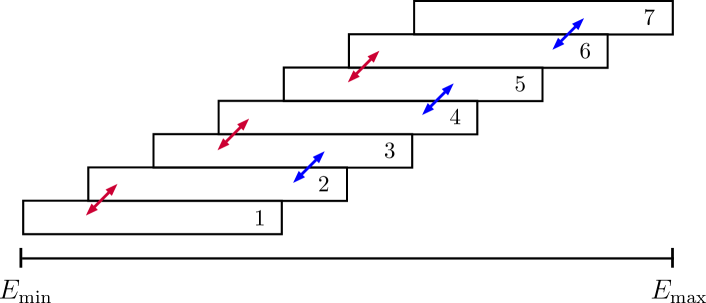
Figure 1: Partitioning the global energy range into seven windows with overlap $o=75\%$. The arrows indicate the communication pathways between neighboring windows for the replica-exchange attempts.

II.3 Monte Carlo trial moves for coupled spin–lattice systems

For coupled spin–lattice systems, the configurational space that one seeks to sample via MC methods consists of $2N$ phase variables: $\{\mathbf{x}\}=\allowbreak\{\mathbf{r}_{1},\allowbreak\mathbf{r}_{2},\cdots,\mathbf{r}_{N},\allowbreak\mathbf{e}_{1},\allowbreak\mathbf{e}_{2},\allowbreak\cdots,\mathbf{e}_{N}\}$. For effectively sampling this configurational space with respect to both the atomic coordinates and the spins, we employ the following two trial moves.

1. Single atom displacement move
   Displace the chosen atom $i$ to a random position $\mathbf{r}_{i}^{\prime}$ within a sphere centered at its original position $\mathbf{r}_{i}$:
   $\mathbf{r}_{i}^{\prime}=\mathbf{r}_{i}+\mathbf{R}$, where $|\mathbf{R}|<R_{\text{max}}$

2. Single spin rotation move
   Assign a new random direction to the spin of the chosen atom $i$.

During each MC step, we randomly choose an atom and perform one of the above trial moves at random with equal probability. Completion of $2N$ such MC steps constitutes a single “MC sweep”.

III Results

Our simulations were performed on a cubic cell of size $L=20$ ($16000$ atoms; 2 atoms per unit cell) with periodic boundary conditions. To explore the sensitivity of the results to the particular choice of EAM potential, we performed simulations using both Dudarev–Derlet (DD) and the Finnis–Sinclair (FS) potentials Dudarev and Derlet (2005); Derlet and Dudarev (2007); Finnis and Sinclair (1984, 1986). The corresponding global energy ranges were chosen to be [$-67200$ eV, $-63200$ eV] and [$-67200$ eV, $-62080$ eV], respectively, for the DD and FS potentials. For both cases, $189$ energy windows with an overlap $o=75\%$ were used, and a single walker per window ($m=1$) was employed. To discretize the energy space, each window was divided into $2000$ energy bins. Replica exchanges between neighboring windows were proposed every $60$ MC sweeps. With these simulation parameters, we observed acceptance rates for the replica exchanges in the range of $49-55\%$. For checking the convergence of $g(E)$, an $80\%$ flatness criterion and a final modification factor of $\text{ln}\,f_{\text{final}}=1\times 10^{-8}$ were used. For both potentials, the full convergence of $g(E)$ was achieved in about $1\times 10^{8}$ MC sweeps, which took less than a week on a $128$GB-RAM AMD Opteron cluster with InfiniBand connectivity.

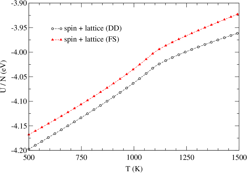
Figure 2: Comparison of the temperature dependence of the internal energy for coupled spin–lattice systems of size $L=20$ using the Dudarev-Derlet [“spin + lattice (DD)”] and Finnis-Sinclair [“spin + lattice (FS)”] potentials. Error bars are smaller than the symbols.

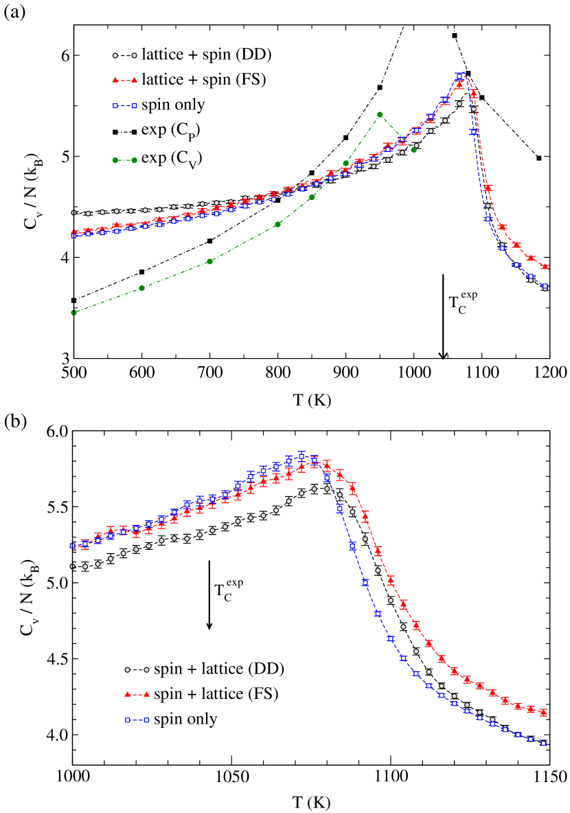
Figure 3: Specific heat as a function of temperature for $L=20$ with [“spin + lattice (DD)” and “spin + lattice (FS)”] and without [“spin only”] the influence of the lattice vibrations; (a) expanded temperature range ${[500\text{\,K},1200\text{\,K}]}$ including the experimental results for $C_{P}$ obtained from Ref. White and Minges (1997) and the corresponding $C_{V}$ values calculated from the $C_{P}$ data; (b) a close-up view in the vicinity of the peak positions. The vertical arrows in both (a) and (b) mark the Curie temperature $T_{C}^{\text{exp}}\approx 1043$ K as predicted by the peak position of the experimental $C_{P}$ curve.

To reduce statistical fluctuations in the estimated thermodynamic quantities, we averaged over the results of $15$ independent runs for the DD potential, and $11$ runs for the FS potential. Fig. 2 shows the comparison of the temperature dependence of the internal energy per atom obtained for the two potentials. For the whole temperature range considered, the internal energy per atom obtained for the FS potential is approximately $0.03$–$0.04$ eV higher than that for the DD potential. Fig. 3 shows the specific heat curves for the two potentials, along with the results obtained from rigid lattice (spin only) simulations in which the atoms were held fixed at perfect bcc lattice positions Perera et al. (2015). Also shown in the subset (a) are the experimental results for the constant-pressure heat capacity $C_{P}$, and the corresponding $C_{V}$ values calculated from the $C_{P}$ data White and Minges (1997) using the relation $C_{V}=C_{P}-VT\alpha^{2}/\beta_{T}$, where $\alpha$ and $\beta_{T}$ are the thermal expansion coefficient and the isothermal compressibility, respectively. Due to the lack of thermal expansion coefficient data, $C_{V}$ values above $1000$ K are not given White and Minges (1997). For a fair comparison with the experimental results, we have added $\frac{3}{2}k_{B}$ to the DD and FS results to include the contribution of the kinetic energy based on the equipartition theorem. For the rigid lattice results, $3k_{B}$ was added to include the contribution of both the kinetic energy and the lattice potential energy. The vertical arrows in both (a) and (b) mark the Curie temperature $T_{C}^{\text{exp}}\approx 1043$ K as predicted by the peak position of the experimental $C_{P}$ curve. The difference between the results for the two different embedded atom potentials is clearly larger than the respective error bars, but both sets of results differ markedly from the estimated values of $C_{V}$ extracted from experiment. The peak in the specific heat corresponding to the rigid lattice simulations is approximately $30$ K higher than the experimental Curie temperature. The introduction of lattice vibrations further pushes the peak position to higher temperatures by several degrees. Moreover, lattice vibrations reduces the amplitude of the peak, an effect which is more pronounced for the case of the DD potential. Specific heat data for the simple cubic Heisenberg ferromagnet Peczak et al. (1991) has shown that the location of the specific heat peak increases as $\sim 0.7L^{-1/0.7}$. Hence, extrapolation of our data to infinite size would change the result very little, as also indicated by exemplary simulations at other system sizes.

IV Summary

In conclusion, we have performed highly parallel replica-exchange Wang–Landau simulations to investigate the magnetic phase transition in a coupled spin–lattice model parameterized for bcc iron. The high level of precision achieved in our simulations has allowed us to make careful comparisons between the results obtained for two different interatomic potentials (FS and DD), and simulations performed on rigid lattices. Such a comprehensive analysis was only possible due to the significant speedup rendered by the parallel, replica-exchange scheme, without any loss of accuracy or precision. While the complete analysis presented in this paper would take of the order of $100$ years for the serial Wang–Landau method performed on a single core processor, we obtained all the results within a few months using the parallel scheme.

Our results indicate that the presence of lattice vibrations only marginally effects the transition temperature and the amplitude of the peak in the specific heat curve. This suggests that the classical Heisenberg model already provides a reasonable depiction of the magnetic phase transition in bcc iron. We also find that the results are sensitive to the particular choice of the interatomic potential, particularly at temperatures further away from the critical temperature $T_{c}$. As the temperature increases beyond $T_{c}$, the specific heat obtained using the FS potential gradually deviates from that of the rigid lattice simulations, whereas below $T_{c}$, a reasonable agreement with the rigid lattice results can be observed. In contrast, the specific heat obtained using the DD potential is higher than that of the rigid lattice simulations up to about $T=800$ K, then remains smaller in comparison to the rigid lattice results until about $T=1100$ K, and thereafter starts to gradually converge with the rigid lattice results. The differences in the results for the two EAM potentials can be attributed to the subtle differences in the ways which the anharmonic effects are captured in these potentials which, in turn, effect the magnetic properties of the system via spin-lattice coupling.