Higher-order organization of complex networks

Networks are a fundamental tool for understanding and modeling complex systems in physics, biology, neuroscience, engineering, and social science. Many networks are known to exhibit rich, lower-order connectivity patterns that can be captured at the level of individual nodes and edges. However, higher-order organization of complex networks—at the level of small network subgraphs—remains largely unknown. Here we develop a generalized framework for clustering networks based on higher-order connectivity patterns. This framework provides mathematical guarantees on the optimality of obtained clusters and scales to networks with billions of edges. The framework reveals higher-order organization in a number of networks including information propagation units in neuronal networks and hub structure in transportation networks. Results show that networks exhibit rich higher-order organizational structures that are exposed by clustering based on higher-order connectivity patterns.

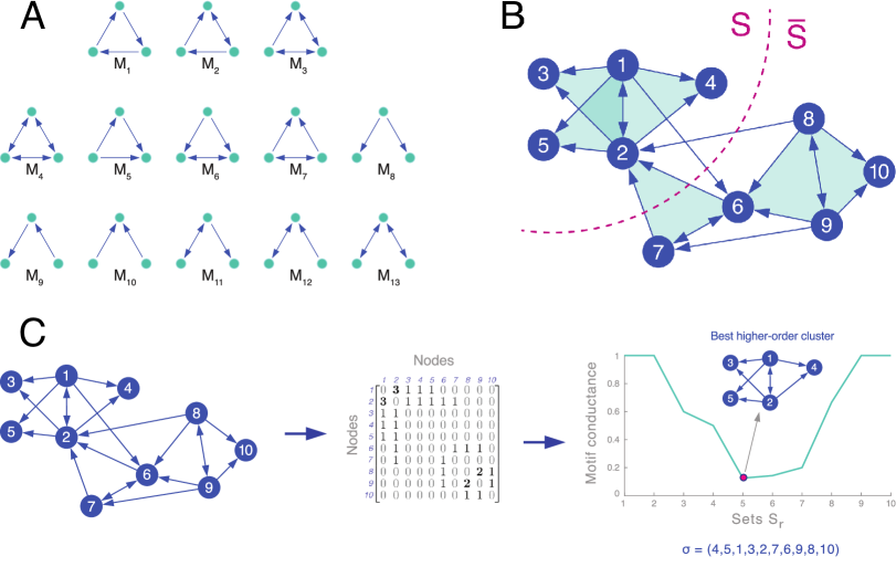
Figure 1: Higher-order network structures and the higher-order network clustering framework. A: Higher-order structures are captured by network motifs. For example, all 13 connected three-node directed motifs are shown here. B: Clustering of a network based on motif $M_{7}$. For a given motif $M$, our framework aims to find a set of nodes $S$ that minimizes motif conductance, $\phi_{M}(S)$, which we define as the ratio of the number of motifs cut (filled triangles cut) to the minimum number of nodes in instances of the motif in either $S$ or $\bar{S}$  (?). In this case, there is one motif cut. C: The higher-order network clustering framework. Given a graph and a motif of interest (in this case, $M_{7}$), the framework forms a motif adjacency matrix ($W_{M}$) by counting the number of times two nodes co-occur in an instance of the motif. An eigenvector of a Laplacian transformation of the motif adjacency matrix is then computed. The ordering $\sigma$ of the nodes provided by the components of the eigenvector  (?) produces nested sets $S_{r}=\{\sigma_{1},\ldots,\sigma_{r}\}$ of increasing size $r$. We prove that the set $S_{r}$ with the smallest motif-based conductance, $\phi_{M}(S_{r})$, is a near-optimal higher-order cluster  (?).

Networks are a standard representation of data throughout the sciences, and higher-order connectivity patterns are essential to understanding the fundamental structures that control and mediate the behavior of many complex systems  (?, ?, ?, ?, ?, ?, ?). The most common higher-order structures are small network subgraphs, which we refer to as network motifs (Figure 1A). Network motifs are considered building blocks for complex networks  (?, ?). For example, feedforward loops (Figure 1A $M_{5}$) have proven fundamental to understanding transcriptional regulation networks  (?), triangular motifs (Figure 1A $M_{1}$–$M_{7}$) are crucial for social networks  (?), open bidirectional wedges (Figure 1A $M_{13}$) are key to structural hubs in the brain  (?), and two-hop paths (Figure 1A $M_{8}$–$M_{13}$) are essential to understanding air traffic patterns  (?). While network motifs have been recognized as fundamental units of networks, the higher-order organization of networks at the level of network motifs largely remains an open question.

Here we use higher-order network structures to gain new insights into the organization of complex systems. We develop a framework that identifies clusters of network motifs. For each network motif (Figure 1A), a different higher-order clustering may be revealed (Figure 1B), which means that different organizational patterns are exposed depending on the chosen motif.

Conceptually, given a network motif $M$, our framework searches for a cluster of nodes $S$ with two goals. First, the nodes in $S$ should participate in many instances of $M$. Second, the set $S$ should avoid cutting instances of $M$, which occurs when only a subset of the nodes from a motif are in the set $S$ (Figure 1B). More precisely, given a motif $M$, the higher-order clustering framework aims to find a cluster (defined by a set of nodes $S$) that minimizes the following ratio:

$$\phi_{M}(S)=\text{cut}_{M}(S,\bar{S})/\min(\text{vol}_{M}(S),\text{vol}_{M}(\bar{S})),$$ (1)

where $\bar{S}$ denotes the remainder of the nodes (the complement of $S$), $\text{cut}_{M}(S,\bar{S})$ is the number of instances of motif $M$ with at least one node in $S$ and one in $\bar{S}$, and $\text{vol}_{M}(S)$ is the number of nodes in instances of $M$ that reside in $S$. Equation 1 is a generalization of the conductance metric in spectral graph theory, one of the most useful graph partitioning scores  (?). We refer to $\phi_{M}(S)$ as the motif conductance of $S$ with respect to $M$.

Finding the exact set of nodes $S$ that minimizes the motif conductance is computationally infeasible  (?). To approximately minimize Equation 1 and hence identify higher-order clusters, we develop an optimization framework that provably finds near-optimal clusters (Supplementary Materials  (?)). We extend the spectral graph clustering methodology, which is based on the eigenvalues and eigenvectors of matrices associated with the graph  (?), to account for higher-order structures in networks. The resulting method maintains the properties of traditional spectral graph clustering: computational efficiency, ease of implementation, and mathematical guarantees on the near-optimality of obtained clusters. Specifically, the clusters identified by our higher-order clustering framework satisfy the motif Cheeger inequality  (?), which means that our optimization framework finds clusters that are at most a quadratic factor away from optimal.

The algorithm (illustrated in Figure 1C) efficiently identifies a cluster of nodes $S$ as follows:

• Step 1: Given a network and a motif $M$ of interest, form the motif adjacency matrix $W_{M}$ whose entries $(i,j)$ are the co-occurrence counts of nodes $i$ and $j$ in the motif $M$:

  $$(W_{M})_{ij}=\text{number of instances of $M$ that contain nodes $i$ and $j$}.$$ (2)

• Step 2: Compute the spectral ordering $\sigma$ of the nodes from the normalized motif Laplacian matrix constructed via $W_{M}$  (?).

• Step 3: Find the prefix set of $\sigma$ with the smallest motif conductance, formally: $S:=\arg\min_{r}\phi_{M}(S_{r})$, where $S_{r}=\{\sigma_{1},\ldots,\sigma_{r}\}$.

For triangular motifs, the algorithm scales to networks with billions of edges and typically only takes several hours to process graphs of such size. On smaller networks with hundreds of thousands of edges, the algorithm can process motifs up to size 9  (?). While the worst-case computational complexity of the algorithm for triangular motifs is $\Theta(m^{1.5})$ , where $m$ is the number of edges in the network, in practice the algorithm is much faster. By analyzing 16 real-world networks where the number of edges $m$ ranges from 159,000 to 2 billion we found the computational complexity to scale as $\Theta(m^{1.2})$. Moreover, the algorithm can easily be parallelized and sampling techniques can be used to further improve performance  (?).

The framework can be applied to directed, undirected, and weighted networks as well as motifs  (?). Moreover, it can also be applied to networks with positive and negative signs on the edges, which are common in social networks (friend vs. foe or trust vs. distrust edges) and metabolic networks (edges signifying activation vs. inhibition)  (?). The framework can be used to identify higher-order structure in networks where domain knowledge suggests the motif of interest. In the Supplementary Material  (?) we also show that when domain-specific higher-order pattern is not known in advance, the framework can also serve to identify which motifs are important for the modular organization of a given network  (?). Such a general framework allows for a study of complex higher-order organizational structures in a number of different networks using individual motifs and sets of motifs. The framework and mathematical theory immediately extend to other spectral methods such as localized algorithms that find clusters around a seed node  (?) and algorithms for finding overlapping clusters  (?). To find several clusters, one can use embeddings from multiple eigenvectors and $k$-means clustering  (?, ?) or apply recursive bi-partitioning  (?, ?).

The framework can serve to identify higher-order modular organization of networks. We apply the higher-order clustering framework to the C. elegans neuronal network, where the four-node “bi-fan” motif (Figure 2A) is over-expressed  (?). The higher-order clustering framework then reveals the organization of the motif within the C. elegans neuronal network. We find a cluster of 20 neurons in the frontal section with low bi-fan motif conductance (Figure 2B). The cluster shows a way that nictation is controlled. Within the cluster, ring motor neurons (RMEL/V/R), proposed pioneers of the nerve ring  (?), propagate information to IL2 neurons, regulators of nictation  (?), through the neuron RIH and several inner labial sensory neurons (Figure 2C). Our framework contextualizes the sifnifance of the bi-fan motif in this control mechanism.

The framework also provides new insights into network organization beyond the clustering of nodes based only on edges. Results on a transportation reachability network  (?) demonstrate how it finds the essential hub interconnection airports (Figure 3). These appear as extrema on the primary spectral direction (Figure 3C) when two-hop motifs (Figure 3A) are used to capture highly connected nodes and non-hubs. (The first spectral coordinate of the normalized motif Laplacian embedding was positively correlated with the airport city’s metropolitan population with Pearson correlation 99% confidence interval [0.33, 0.53]). The secondary spectral direction identified the West-East geography in the North American flight network (it was negatively correlated with the airport city’s longitude with Pearson correlation 99% confidence interval [-0.66, -0.50]). On the other hand, edge-based methods conflate geography and hub structure. For example, Atlanta, a large hub, is embedded next to Salina, a non-hub, with an edge-based method (Figure 3D).

Our higher-order network clustering framework unifies motif analysis and network partitioning—two fundamental tools in network science—and reveals new organizational patterns and modules in complex systems. Prior efforts along these lines do not provide worst-case performance guarantees on the obtained clustering  (?), do not reveal which motifs organize the network  (?), or rely on expanding the size of the network  (?, ?). Theoretical results in the Supplementary Material  (?) also explain why classes of hypergraph partitioning methods are more general than previously assumed and how motif-based clustering provides a rigorous framework for the special case of partitioning directed graphs. Finally, the higher-order network clustering framework is generally applicable to a wide range of networks types, including directed, undirected, weighted, and signed networks.

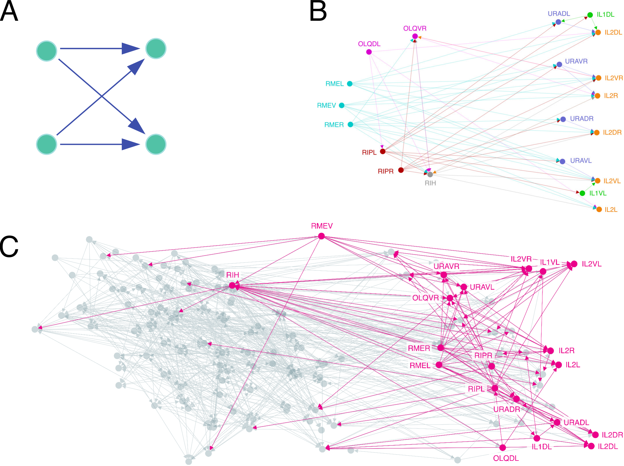
Figure 2: Higher-order cluster in the C. elegans neuronal network  (?). A: The 4-node “bi-fan” motif, which is over-expressed in neuronal networks  (?). Intuitively, this motif describes a cooperative propagation of information from the nodes on the left to the nodes on the right. B: The best higher-order cluster in the C. elegans frontal neuronal network based on the motif in (A). The cluster contains three ring motor neurons (RMEL/V/R; cyan) with many outgoing connections, serving as the source of information; six inner labial sensory neurons (IL2DL/VR/R/DR/VL; orange) with many incoming connections, serving as the destination of information; and four URA neurons (purple) acting as intermediaries. These RME neurons have been proposed as pioneers for the nerve ring  (?), while the IL2 neurons are known regulators of nictation  (?), and the higher-order cluster exposes their organization. The cluster also reveals that RIH serves as a critical intermediary of information processing. This neuron has incoming links from all three RME neurons, outgoing connections to five of the six IL2 neurons, and the largest total number of connections of any neuron in the cluster. C: Illustration of the higher-order cluster in the context of the entire network. Node locations are the true two-dimensional spatial embedding of the neurons. Most information flows from left to right, and we see that RME/V/R/L and RIH serve as sources of information to the neurons on the right.

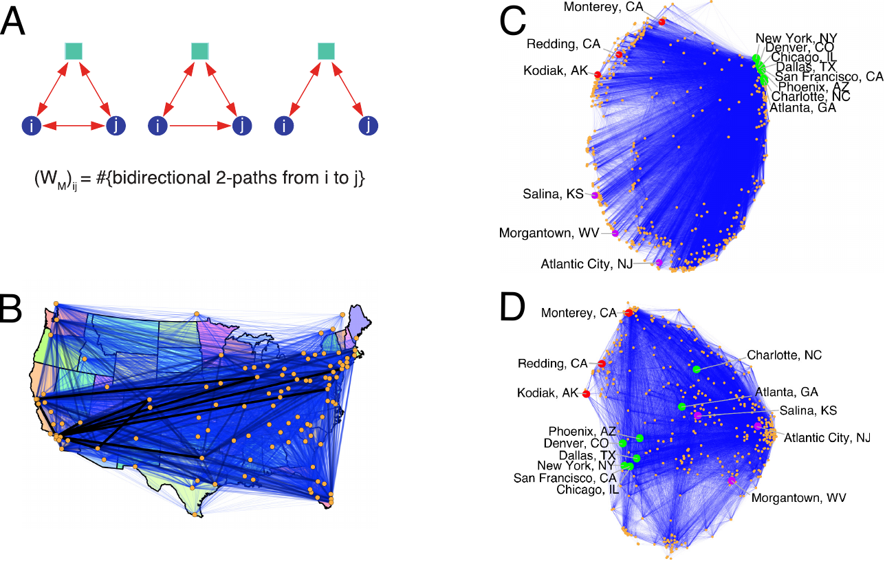
Figure 3: Higher-order spectral analysis of a network of airports in Canada and the United States  (?). A: The three higher-order structures used in our analysis. Each motif is “anchored” by the blue nodes $i$ and $j$, which means our framework only seeks to cluster together the blue nodes. Specifically, the motif adjacency matrix adds weight to the $(i,j)$ edge based on the number of third intermediary nodes (green squares). The first two motifs correspond to highly-connected cities and the motif on the right connects non-hubs to non-hubs. B: The top 50 most populous cities in the United States which correspond to nodes in the network. The edge thickness is proportional to the weight in the motif adjacency matrix $W_{M}$. The thick, dark lines indicate that large weights correspond to popular mainline routes. C: Embedding of nodes provided by their corresponding components of the first two non-trivial eigenvectors of the normalized Laplacian for $W_{M}$. The marked cities are eight large U.S. hubs (green), three West coast non-hubs (red), and three East coast non-hubs (purple). The primary spectral coordinate (left to right) reveals how much of a hub the city is, and the second spectral coordinate (top to bottom) captures West-East geography  (?). D: Embedding of nodes provided by their corresponding components in the first two non-trivial eigenvectors of the standard, edge-based (non-higher-order) normalized Laplacian. This method does not capture the hub and geography found by the higher-order method. For example, Atlanta, the largest hub, is in the center of the embedding, next to Salina, a non-hub.

S1 Derivation and analysis of the motif-based spectral clustering method

We now cover the background and theory for deriving and understanding the method presented in the main text. We will start by reviewing the graph Laplacian and cut and volume measures for sets of vertices in a graph. We then define network motifs in Section S1.2 and generalizes the notions of cut and volume to motifs. Our new theory is presented in Section S1.6 and then we summarize some extensions of the method. Finally, we relate our method to existing methods for directed graph clustering and hypergraph partitioning.

S1.1 Review of the graph Laplacian for weighted, undirected graphs

Consider a weighted, undirected graph $G=(V,E)$, with $\lvert V\rvert=n$. Further assume that $G$ has no isolated nodes. Let $W$ encode the weights, of the graph, i.e., $W_{ij}=W_{ji}=\text{weight of edge (i, j)}$. The diagonal degree matrix $D$ is defined as $D_{ii}=\sum_{j=1}^{n}W_{ij}$, and the graph Laplacian is defined as $L=D-W$. We now relate these matrices to the conductance of a set $S$, $\phi^{(G)}(S)$:

$$\phi^{(G)}(S) = \textnormal{cut}^{(G)}(S,\bar{S})/\min(\textnormal{vol}^{(G)}(S),\textnormal{vol}^{(G)}(\bar{S})),$$ (S3)

$$\textnormal{cut}^{(G)}(S,\bar{S}) = \sum_{i\in S,\;j\in\bar{S}}W_{ij},$$ (S4)

$$\textnormal{vol}^{(G)}(S) = \sum_{i\in S}D_{ii}$$ (S5)

Here, $\bar{S}=V\backslash S$. (Note that conductance is a symmetric measure in $S$ and $\bar{S}$, i.e., $\phi^{(G)}(S)=\phi^{(G)}(\bar{S})$.) Conceptually, the cut and volume measures are defined as follows:

$$\textnormal{cut}^{(G)}(S,\bar{S}) =$$ weighted sum of weights of edges that are cut (S6)

$$\textnormal{vol}^{(G)}(S) = S$$ weighted number of edge end points in (S7)

Since we have assumed $G$ has no isolated nodes, $\textnormal{vol}^{(G)}(S)>0$. If $G$ is disconnected, then for any connected component $C$, $\phi^{(G)}(C)=0$. Thus, we usually consider breaking $G$ into connected components as a pre-processing step for algorithms that try to find low-conductance sets.

We now relate the cut metric to a quadratic form on $L$. Later, we will derive a similar form for a motif cut measure. Note that for any vector $y\in\mathbb{R}^{n}$,

$$y^{T}Ly=\sum_{(i,j)\in E}w_{ij}(y_{i}-y_{j})^{2}.$$ (S8)

Now, define $x$ to be an indicator vector for a set of nodes $S$ i.e., $x_{i}=1$ if node $i$ is in $S$ and $x_{i}=0$ if node $i$ is in $\bar{S}$. Note that if an edge $(i,j)$ is cut, then $x_{i}$ and $x_{j}$ take different values and $(x_{i}-x_{j})^{2}=1$; otherwise, $(x_{i}-x_{j})^{2}=0$. Thus,

$$x^{T}Lx=\textnormal{cut}^{(G)}(S,\bar{S}).$$ (S9)

S1.2 Definition of network motifs

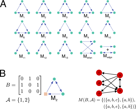
Figure S4: A: Illustration of network motifs used throughout the main text and supplementary material. The motif $M_{\textnormal{edge}}$ is used to represent equivalence to undirected the graph. B: Diagram of motif definitions. The motif is defined by a binary matrix $B$ and an anchor set of nodes. The figure shows an anchored version of motif $M_{2}$ with anchors on the nodes that form the bi-directional edge. There are two instances of the motif in the graph on the right. Note that $(\{a,b,d\},\{a,b\})$ is not included in the set of motif instances because the induced subgraph on the nodes $a$, $b$, and $d$ is not isomorphic to the graph defined by $B$.

We now define network motifs as used in our work. We note that there are alternative definitions in the literature  (?). We consider motifs to be a pattern of edges on a small number of nodes (see Figure S4). Formally, we define a motif on $k$ nodes by a tuple $(B,\mathcal{A})$, where $B$ is a $k\times k$ binary matrix and $\mathcal{A}\subset\{1,2,\ldots,k\}$ is a set of anchor nodes. The matrix $B$ encodes the edge pattern between the $k$ nodes, and $\mathcal{A}$ labels a relevant subset of nodes for defining motif conductance. In many cases, $\mathcal{A}$ is the entire set of nodes. Let $\chi_{\mathcal{A}}$ be a selection function that takes the subset of a $k$-tuple indexed by $\mathcal{A}$, and let $\text{set}(\cdot)$ be the operator that takes an (ordered) tuple to an (unordered) set. Specifically,

$$\text{set}((v_{1},v_{2},\ldots,v_{k}))=\{v_{1},v_{2},\ldots,v_{k}\}.$$

The set of motifs in an unweighted (possibly directed) graph with adjacency matrix $A$, denoted $M(B,\mathcal{A})$, is defined by

$$M(B,\mathcal{A})=\{(\text{set}(\bm{v}),\text{set}(\chi_{\mathcal{A}}(\bm{v})))\;\mid\;\bm{v}\in V^{k},\quad v_{1},\ldots,v_{k}\text{ distinct},\quad A_{\bm{v}}=B\},$$ (S10)

where $A_{\bm{v}}$ is the $k\times k$ adjacency matrix on the subgraph induced by the $k$ nodes of the ordered vector $\bm{v}$. Figure S4 illustrates these definitions. The set operator is a convenient way to avoid duplicates when defining $M(B,\mathcal{A})$ for motifs exhibiting symmetries. Henceforth, we will just use $(\bm{v},\chi_{\mathcal{A}}(\bm{v}))$ to denote $(\text{set}(\bm{v}),\text{set}(\chi_{\mathcal{A}}(\bm{v})))$ when discussing elements of $M(B,\mathcal{A})$. Furthermore, we call any $(\bm{v},\chi_{\mathcal{A}}(\bm{v}))\in M(B,\mathcal{A})$ a motif instance. When $B$ and $\mathcal{A}$ are arbitrary or clear from context, we will simply denote the motif set by $M$.

We call motifs where $\chi_{\mathcal{A}}(\bm{v})=\bm{v}$ simple motifs and motifs where $\chi_{\mathcal{A}}(\bm{v})\neq\bm{v}$ anchored motifs. Motif analysis in the literature has mostly analyzed simple motifs  (?). However, the anchored motif provides us with a more general framework, and we use an anchored motif for the analysis of the transportation reachability network.

Often, a distinction is made between a functional and a structural motif  (?) (or a subgraph and an induced subgraph  (?)) to distinguish whether a motif specifies simply the existence of a set of edges (functional motif or subgraph) or the existence and non-existence of edges (structural motif or induced subgraph). By the definition in Equation S10, we refer to structural motifs in this work. Note that functional motifs consist of a set of structural motifs. Our clustering framework allows for the simultaneous consideration of several motifs (see Section S1.9), so we have not lost any generality in our definitions.

S1.3 Definition of motif conductance

Recall that the key definitions for defining conductance are the notions of cut and volume. For an unweighted graph, these are

$$\phi^{(G)}(S,\bar{S}) = \textnormal{cut}^{(G)}(S,\bar{S})/\min(\textnormal{vol}^{(G)}(S),\textnormal{vol}^{(G)}(\bar{S})),$$ (S11)

$$\textnormal{cut}^{(G)}(S,\bar{S}) = \text{number of edges cut},$$ (S12)

$$\textnormal{vol}^{(G)}(S) = \text{number of edge end points in $S$}.$$ (S13)

Our conceptual definition of motif conductance simply replaces an edge with a motif instance of type $M$:

$$\phi^{(G)}_{M}(S) = \textnormal{cut}^{(G)}_{M}(S,\bar{S})/\min(\textnormal{vol}^{(G)}_{M}(S),\textnormal{vol}^{(G)}_{M}(\bar{S})),$$ (S14)

$$\textnormal{cut}^{(G)}_{M}(S,\bar{S}) = \text{number of motif instances cut},$$ (S15)

$$\textnormal{vol}^{(G)}_{M}(S) = \text{number of motif instance end points in $S$}.$$ (S16)

We say that a motif instance is cut if there is at least one anchor node in $S$ and at least one anchor node in $\bar{S}$. We can formalize this when given a motif set $M$ as in Equation S10:

$$\textnormal{cut}^{(G)}_{M}(S,\bar{S}) = \sum_{(\bm{v},\chi_{\mathcal{A}}(\bm{v}))\in M}\operatorname{\textbf{1}}(\exists\;i,j\in\chi_{\mathcal{A}}(\bm{v})\;\mid\;i\in S,j\in\bar{S}),$$ (S17)

$$\textnormal{vol}^{(G)}_{M}(S) = \sum_{(\bm{v},\chi_{\mathcal{A}}(\bm{v}))\in M}\sum_{i\in\chi_{\mathcal{A}}(\bm{v})}\operatorname{\textbf{1}}(i\in S),$$ (S18)

where $\operatorname{\textbf{1}}(s)$ is the truth-value indicator function on $s$, i.e., $\operatorname{\textbf{1}}(s)$ takes the value $1$ if the statement $s$ is true and $0$ otherwise. Note that Equation S17 makes explicit use of the anchor set $\mathcal{A}$. The motif cut measure only counts an instance of a motif as cut if the anchor nodes are separated, and the motif volume counts the number of anchored nodes in the set. However, two nodes in an achor set may a part of several motif instances. Specifically, following the definition in Equation S10, there may be many different $\bm{v}$ with the same $\chi_{\mathcal{A}}(\bm{v})$, and the nodes in $\chi_{\mathcal{A}}(\bm{v})$ still get counted proportional to the number of motif instances.

S1.4 Definition of the motif adjacency matrix and motif Laplacian

Given an unweighted, directed graph and a motif set $M$, we conceptually define the motif adjacency matrix by

$$(W_{M})_{ij}=\text{number of motif instances in $M$ where $i$ and $j$ participate in the motif}.$$ (S19)

Or, formally,

$$(W_{M})_{ij}=\sum_{(\bm{v},\chi_{\mathcal{A}}(\bm{v}))\in M}\operatorname{\textbf{1}}(\{i,j\}\subset\chi_{\mathcal{A}}(\bm{v})),$$ (S20)

for $i\neq j$. Note that weight is added to $(W_{M})_{ij}$ only if $i$ and $j$ appear in the anchor set. This is important for the transportation reachability network analyzed in the main text and in Section S6, where weight is added between cities $i$ and $j$ based on the number of intermediary cities that can be traversed between them.

Next, we define the motif diagonal degree matrix by $(D_{M})_{ii}=\sum_{j=1}^{n}(W_{M})_{ij}$ and the motif Laplacian as $L_{M}=D_{M}-W_{M}$. Finally, the normalized motif Laplacian is $\mathcal{L}_{M}=D_{M}^{-1/2}L_{M}D_{M}^{-1/2}=I-D_{M}^{-1/2}W_{M}D_{M}^{-1/2}$. The theory in the next section will examine quadratic forms $L_{M}$ and derive the main clustering method that uses an eigenvector of $\mathcal{L}_{M}$.

S1.5 Algorithm for finding a single cluster

We are now ready to describe the algorithm for finding a single cluster in a graph. The algorithm finds a partition of the nodes into $S$ and $\bar{S}$. The motif conductance is symmetric in the sense that $\phi^{(G)}_{M}(S)=\phi^{(G)}_{M}(\bar{S})$, so either set of nodes ($S$ or $\bar{S}$) could be interpreted as a cluster. However, in practice, it is common that one set is substantially smaller than the other. We consider this smaller set to represent a module in the network. The algorithm is based on the Fiedler partition  (?) of the motif weighted adjacency matrix and is presented below in Algorithm 1.

Input: Directed, unweighted graph $G$ and motif $M$

Output: Motif-based cluster (subset of nodes in $G$)

$(W_{M})_{ij}\leftarrow\text{number of instances of $M$ that contain nodes $i$ and $j$}.$

$G_{M}\leftarrow$ weighted graph induced $W_{M}$

$D_{M}\leftarrow$ diagonal matrix with $(D_{M})_{ii}=\sum_{j}(W_{M})_{ij}$

$z\leftarrow$ eigenvector of second smallest eigenvalue for $\mathcal{L}_{M}=I-D_{M}^{-1/2}W_{M}D_{M}^{-1/2}$

$\sigma_{i}\leftarrow$ to be index of $D_{M}^{-1/2}z$ with $i$th smallest value

/* Sweep over all prefixes of $\sigma$ */

$S\leftarrow\arg\min_{l}\phi^{(G_{M})}(S_{l})$, where $S_{l}=\{\sigma_{1},\ldots,\sigma_{l}\}$

if $\lvert S\rvert<\lvert\bar{S}\rvert$ then

       return $S$

      

else

       return $\bar{S}$

      

Algorithm 1 Motif-based clustering algorithm for finding a single cluster.

It is often informative to look at all conductance values found from the sweep procedure. We refer to a plot of $\phi^{(G_{M})}(S_{l})$ versus $l$ as a sweep profile plot. In the following subection, we show that when the motif has three nodes, $\phi^{(G_{M})}(S_{l})=\phi^{(G)}_{M}(S_{l})$. In this case, the sweep profile shows how motif conductance varies with the size of the sets in Algorithm 1.

In the following subsection, we show that when the motif $M$ has three nodes, the cluster satisfies $\phi^{(G)}_{M}(S)\leq 4\sqrt{\phi^{*}}$, where $\phi^{*}$ is the smallest motif conductance over all sets of nodes. In other words, the cluster is nearly optimal. Later, we extend this algorithm to allow for signed, colored, and weighted motifs and to simultaneously finding multiple clusters.

S1.6 Motif Cheeger inequality for network motifs with three nodes

We now derive the motif Cheeger inequality for simple three-node motifs, or, in general, motifs with three anchor nodes. The crux of this result is deriving a relationship between the motif conductance function and the weighted motif adjacency matrix, from which the Cheeger inequality is essentially a corollary. For the rest of this section, we will use the following notation. Given an unweighted, directed $G$ and a motif $M$, the corresponding weighted graph defined by Equation S20 is denoted by $G_{M}$.

The following Lemma relates the motif volume to the volume in the weighted graph. This lemma applies to any anchor set $\mathcal{A}$ consisting of at least two nodes. For our main result, we will apply the lemma assuming $|\mathcal{A}|=3$. However, we will apply the lemma more generally when discussing four node motifs in Section S1.7.

Lemma 1.

Let $G=(V,E)$ be a directed, unweighted graph and let $G_{M}$ be the weighted graph for a motif on $k$ nodes and $|\mathcal{A}|\geq 2$ anchor nodes. Then for any $S\subset V$,

$$\textnormal{vol}^{(G)}_{M}(S)=\frac{1}{|\mathcal{A}|-1}\textnormal{vol}^{(G_{M})}(S)$$

Proof.

Consider an instance $(\bm{v},\chi_{\mathcal{A}}(\bm{v}))$ of a motif. Let $(u_{1},\ldots,u_{|\mathcal{A}|})=\chi_{\mathcal{A}}(\bm{v})$. By Equation S20, $(W_{M})_{u_{1},j}$ is incremented by one for $j=u_{2},\ldots,u_{|\mathcal{A}|}$. Since $(D_{M})_{u_{1},u_{1}}=\sum_{j}{(W_{M})_{u_{1},j}}$, the motif end point $u_{1}$ is counted $|\mathcal{A}|-1$ times. ∎

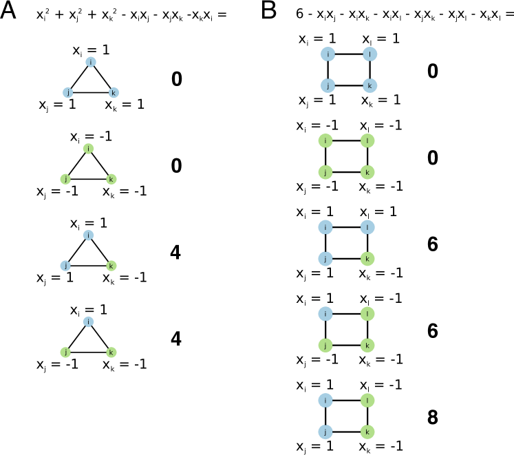
Figure S5: Illustrations of the quadratic forms on indicator functions for set assignment. Here, the blue nodes have assignment to set $S$ and the green nodes have assignment to set $\bar{S}$. The quadratic function gives the penalty for cutting that motif. A: Illustration of Equation 2. The quadratic form is proportional to the indicator on whether or not the motif is cut. B: Illustration of Equation S25. The quadratic form is equal to zero when all nodes are in the same set. However, the form penalizes 2/2 splits more than 3/1 splits.

The following lemma states that the truth value for determining whether three binary variables in $\{-1,1\}$ are not all equal is a quadratic function of the variables (see Figure S5). Because this function is quadratic, we will be able to relate motif cuts on three nodes to a quadratic form on the motif Laplacian.

Lemma 2.

Let $x_{i},x_{j},x_{k}\in\{-1,1\}$. Then

$$4\cdot\operatorname{\textbf{1}}(x_{i},x_{j},x_{k}\text{ not all the same})=x_{i}^{2}+x_{j}^{2}+x_{k}^{2}-x_{i}x_{j}-x_{j}x_{k}-x_{k}x_{i}.$$

It will be easier to derive our results with binary indicator variables taking values in $\{-1,1\}$. However, in terms of the quadratic form on the Laplacian, we have already seen how indicator vectors taking values in $\{0,1\}$ relate to the cut value (Equation S9). The following lemma shows that the $\{0,1\}$ and $\{-1,1\}$ indicator vectors are equivalent, up to a constant, for defining the cut measure in terms of the Laplacian.

Lemma 3.

Let $z\in\{0,1\}^{n}$ and define $x$ by $x_{i}=1$ if $z_{i}=1$ and $x_{i}=-1$ if $z_{i}=0$. Then for any graph Laplacian $L=D-W$, $4z^{T}Lz=x^{T}Lx$.

Proof.

$$x^{T}Lx=\sum_{(i,j)\in E}W_{ij}(x_{i}-x_{j})^{2}=\sum_{(i,j)\in E}W_{ij}4(z_{i}-z_{j})^{2}=4z^{T}Lz.$$

∎

The next lemma contains the essential result that relates motif cuts in the original graph $G$ to weighted edge cuts in $G_{M}$. In particular, the lemma shows that the motif cut measure is proportional to the cut on the weighted graph defined in Equation S19 when there are three anchor nodes.

Lemma 4.

Let $G=(V,E)$ be a directed, unweighted graph and let $G_{M}$ be the weighted graph for a motif with $|\mathcal{A}|=3$. Then for any $S\subset V$,

$$\textnormal{cut}^{(G)}_{M}(S,\bar{S})=\frac{1}{2}\textnormal{cut}^{(G_{M})}(S,\bar{S})$$

Proof.

Let $x\in\{-1,1\}^{n}$ be an indicator vector of the node set $S$.

$$4\cdot\textnormal{cut}^{(G)}_{M}(S,\bar{S}) = \sum_{(\bm{v},\{i,j,k\})\in M}4\cdot\operatorname{\textbf{1}}(x_{i},x_{j},x_{k}\text{ not all the same})$$

$$= \sum_{(\bm{v},\{i,j,k\})\in M}\left(x_{i}^{2}+x_{j}^{2}+x_{k}^{2}\right)-\left(x_{i}x_{j}+x_{j}x_{k}+x_{k}x_{i}\right)$$

$$= \frac{1}{2}x^{T}D_{M}x-\frac{1}{2}x^{T}W_{M}x$$

$$= \frac{1}{2}x^{T}L_{M}x$$

$$= 2\cdot\textnormal{cut}^{(G_{M})}(S,\bar{S}).$$

The first equality follows from the definition of cut motifs (Equation S17). The second equality follows from Lemma 2. The third equality follows from Lemma 1 and Equation S20. The fourth equality follows from the definition of $L_{M}$. The fifth equality follows from Lemma 3. ∎

We are now ready to prove our main result, namely that motif conductance on the original graph $G$ is equivalent to conductance on the weighted graph $G_{M}$ when there are three anchor nodes. The result is a consequence of the volume and cut relationships provided by Lemmas 1 and 4.

Theorem 5.

Let $G=(V,E)$ be a directed, unweighted graph and let $W_{M}$ be the weighted adjacency matrix for any motif with $|\mathcal{A}|=3$. Then for any $S\subset V$,

$$\phi^{(G)}_{M}(S)=\phi^{(G_{M})}(S)$$

In other words, when the number of anchor nodes is $3$, the motif conductance is equal to the conductance on the weighted graph defined by Equation S19.

Proof.

When $|\mathcal{A}|=3$, the motif cut and motif volume are both equal to half the motif cut and motif volume measures by Lemmas 1 and 4. ∎

For any motif with three anchor nodes, conductance on the weighted graph is equal to the motif conductance. Because of this, we can use results from spectral graph theory for weighted graphs  (?) and re-interpret the results in terms of motif conductance. In particular, we get the following “motif Cheeger inequality”.

Theorem 6.

Motif Cheeger Inequality. Suppose we use Algorithm 1 to find a low-motif conductance set $S$. Let $\phi_{*}=\min_{S^{\prime}}\phi^{(G)}_{M}(S^{\prime})$ be the optimal motif conductance over any set of nodes $S^{\prime}$. Then

1. $\phi^{(G)}_{M}(S)\leq 4\sqrt{\phi^{*}}$ and

2. $\phi^{*}\geq\lambda_{2}/2$

Proof.

The result follows from Theorem 5 and the standard Cheeger ineqaulity  (?). ∎

The first part of the result says that the set of nodes $S$ is within a quadratic factor of optimal. This provides the mathematical guarantees that our procedure finds a good cluster in a graph, if one exists. The second result provides a lower bound on the optimal motif conductance in terms of the eigenvalue. We use this bound in our analysis of a food web (see Section S7.1) to show that certain motifs do not provide good clusters, regardless of the procedure to select $S$.

S1.7 Discussion of motif Cheeger inequality for network motifs with four or more nodes

Analogs of the indicator function in Lemma 2 for four or more variables are not quadratic. Subsequently, for motifs with $|\mathcal{A}|>3$, we no longer get the motif Cheeger inequalities guaranteed by Theorem 6. That being said, solutions found by motif-based partitioning approximate a related value of conductance. We now provide the details.

We begin with a lemma that shows a functional form for four binary variables taking values in $\{-1,1\}$ to not all be equal. We see that it is quartic, not quadratic.

Lemma 7.

Let $x_{i},x_{j},x_{k},x_{l}\in\{-1,1\}$. Then the indicator function on all four elements not being equal is

$$8\cdot\operatorname{\textbf{1}}(x_{i},x_{j},x_{k},x_{l}\text{ not all the same})$$

$$= \left(7-x_{i}x_{j}-x_{i}x_{k}-x_{i}x_{l}-x_{j}x_{k}-x_{j}x_{l}-x_{k}x_{l}-x_{i}x_{j}x_{k}x_{l}\right).$$

We almost have a quadratic form, if not for the quartic term $x_{i}x_{j}x_{k}x_{l}$. However, we could use the following related quadratic form:

$$6-x_{i}x_{j}-x_{i}x_{k}-x_{i}x_{l}-x_{j}x_{k}-x_{j}x_{l}-x_{k}x_{l}$$

$$=\left\{\begin{array}[]{ll}0&x_{i},x_{j},x_{k},x_{l}\text{ are all the same}\\ 6&\text{exactly three of }x_{i},x_{j},x_{k},x_{l}\text{ are the same}\\ 8&\text{exactly two of }x_{i},x_{j},x_{k},x_{l}\text{ are $-1$}.\end{array}\right.$$ (S25)

The quadratic still takes value $0$ if all four entries are the same, and takes a non-zero value otherwise. However, the quadratic takes a larger value if exactly two of the entries are $-1$. Figure S5 illustrates this idea. From this, we can provide an analogous statement to Lemma 4 for motifs with $|\mathcal{A}|=4$.

Lemma 8.

Let $G=(V,E)$ be a directed, unweighted graph and let $G_{M}$ be the weighted graph for a motif with $|\mathcal{A}|=4$. Then for any $S\subset V$,

$$\textnormal{cut}^{(G)}_{M}(S,\bar{S})=\frac{1}{3}\textnormal{cut}^{(G_{M})}(S,\bar{S})-\sum_{(\bm{v},\{i,j,k,l\})\in M}\frac{1}{3}\cdot\operatorname{\textbf{1}}(\text{exactly two of }i,j,k,l\text{ in }S)$$

Proof.

Let $x\in\{-1,1\}^{n}$ be an indicator vector of the node set $S$.

$$6\cdot\textnormal{cut}^{(G)}_{M}(S,\bar{S})+\sum_{(\bm{v},\{i,j,k,l\})\in M}2\cdot\operatorname{\textbf{1}}(\text{exactly two of }i,j,k,l\text{ in }S)$$

$$= \sum_{(\bm{v},\{i,j,k,l\})\in M}6-x_{i}x_{j}-x_{i}x_{k}-x_{i}x_{l}-x_{j}x_{k}-x_{j}x_{l}-x_{k}x_{l}$$

$$= \sum_{(\bm{v},\{i,j,k,l\})\in M}\frac{3}{2}\left(x_{i}^{2}+x_{j}^{2}+x_{k}^{2}+x_{l}^{2}\right)-\left(x_{i}x_{j}+x_{i}x_{k}+x_{i}x_{l}+x_{j}x_{k}+x_{j}x_{l}+x_{k}x_{l}\right)$$

$$= \frac{1}{2}x^{T}D_{M}x-\frac{1}{2}x^{T}W_{M}x$$

$$= \frac{1}{2}x^{T}L_{M}x$$

$$= 2\cdot\textnormal{cut}^{(G_{M})}(S,\bar{S}).$$

The first equality follows from Equations S17 and S25. The third equality follows from Lemma 1. The fourth equality follows from the definition of $L_{M}$. The fifth equality follows from Lemma 3. ∎

With four anchor nodes, the motif cut in $G$ is slightly different than the weighted cut in the weighted graph $G_{M}$. However, Lemma 1 says that the motif volume in $G$ is still the same as the weighted volume in $G_{M}$. We use this to derive the following result.

Theorem 9.

Let $G=(V,E)$ be a directed, unweighted graph and let $W_{M}$ be the weighted adjacency matrix for any motif with $|\mathcal{A}|=4$. Then for any $S\subset V$,

$$\phi^{(G)}_{M}(S)=\phi^{(G_{M})}(S)-\frac{\sum_{(\bm{v},\{i,j,k,l\})\in M}\operatorname{\textbf{1}}(\text{exactly two of }i,j,k,l\text{ in }S)}{\textnormal{vol}^{(G_{M})}(S)}$$

In other words, when there are four anchor nodes, the weighting scheme in Equation S19 models the exact conductance with an additional penalty for splitting the four anchor nodes into two groups of two.

Proof.

This follows from Lemmas 1 and 8. ∎

To summarize, we still get a Cheeger inequality from the weighted graph, but it is in terms of a penalized version of the motif conductance $\phi^{(G)}_{M}(S)$. However, the penalty makes sense—if the group of four nodes is “more split” (2 and 2 as opposed to 3 and 1), the penalty is larger. When $|\mathcal{A}|>4$, we can derive similar penalized approximations to $\phi^{(G)}_{M}(S)$.

S1.8 Methods for simultaneously finding multiple clusters

For clustering a network into $k>2$ clusters based on motifs, we could recursively cut the graph using the sweep procedure with some stopping criterion  (?). For example, we could continue to cut the largest remaining cluster until the graph is partitioned into some pre-specified number of clusters. We refer to this method as recursive bi-partitioning.

In addition, we can use the following method of Ng et al.  (?).

Input: Directed, unweighted graph $G$, motif $M$, number of clusters $k$

Output: $k$ disjoint motif-based clusters

$(W_{M})_{ij}\leftarrow\text{number of instances of $M$ that contain nodes $i$ and $j$}.$

$D_{M}\leftarrow$ diagonal matrix with $(D_{M})_{ii}=\sum_{j}(W_{M})_{ij}$

$z_{1},\ldots,z_{k}\leftarrow$ eigenvectors of $k$ smallest eigenvalues for $\mathcal{L}_{M}=I-D_{M}^{-1/2}W_{M}D_{M}^{-1/2}$

$Y_{ij}\leftarrow z_{ij}/\sqrt{\sum_{j=1}^{k}z_{ij}^{2}}$

Embed node $i$ into $\mathbb{R}^{k}$ by taking the $i$th row of the matrix $Y$

Run $k$-means clustering on the embedded nodes

Algorithm 2 Motif-based clustering algorithm for finding several clusters.

This method does not have the same Cheeger-like guarantee on quality. However, recent theory shows that by replacing $k$-means with a different clustering algorithm, there is a performance guarantee  (?). While this provides motivation, we use $k$-means for its simplicity and empirical success.

S1.9 Extensions of the method for simultaneously analyzing several network motifs

All of our results carry through when considering several motifs simultaneously. In particular, suppose we are interested in clustering based on motif sets $M_{1},\ldots,M_{q}$ for $q$ different motifs. Further suppose that we want to weight the impact of some motifs more than other motifs. Let $W_{M_{j}}$ be the weighted adjacency matrix for motif $M_{j}$, $j=1,\ldots,q$, and let $\alpha_{j}\geq 0$ be the weight of motif $M_{j}$, then we can form the weighted adjacency matrix

$$W_{M}=\sum_{j=1}^{q}\alpha_{j}W_{M_{j}}.$$ (S26)

Now, the cut and volume measures are simply weighted sums by linearity. Suppose that the $M_{j}$ all have three anchor nodes and let $G_{M}$ be the weighted graph corresponding to $W_{M}$. Then

$$\textnormal{cut}^{(G_{M})}(S,\bar{S})=\sum_{j=1}^{q}\alpha_{j}\textnormal{cut}^{(G)}_{M_{j}}(S,\bar{S}),\quad\textnormal{vol}^{(G_{M})}(S)=\sum_{j=1}^{q}\alpha_{j}\textnormal{vol}^{(G)}_{M_{j}}(S),$$

and Theorem 6 applies to a weighted motif conductance equal to

$$\frac{\sum_{j=1}^{q}\alpha_{j}\textnormal{cut}^{(G)}_{M_{j}}(S,\bar{S})}{\min\left(\sum_{j=1}^{q}\alpha_{j}\textnormal{vol}^{(G)}_{M_{j}}(S),\sum_{j=1}^{q}\alpha_{j}\textnormal{vol}^{(G)}_{M_{j}}(\bar{S})\right)}.$$

S1.10 Extensions of the method to signed, colored, and weighted motifs

Our results easily generalize for signed networks. We only have to generalize Equation S10 by allowing the adjacency matrix $B$ to be signed. Extending the method for motifs where the edges or nodes are “colored” or “labeled” is similar. If the edges are colored, then we again just allow the adjacency matrix $B$ to capture this information. If the nodes in the motif are colored, we only count motif instances with the specified pattern.

We can also generalize the notions of motif cut and motif volume for “weighted motifs”, i.e., each motif has an associated nonnegative weight. Let $\omega_{(\bm{v},\chi_{\mathcal{A}}(\bm{v}))}$ be the weight of a motif instance. Our cut and volume metrics are then

$$\textnormal{cut}^{(G)}_{M}(S,\bar{S}) = \sum_{(\bm{v},\chi_{\mathcal{A}}(\bm{v}))\in M}\omega_{(\bm{v},\chi_{\mathcal{A}}(\bm{v}))}\operatorname{\textbf{1}}(\exists\;i,j\in\chi_{\mathcal{A}}(\bm{v})\;\mid\;i\in S,j\in\bar{S}),$$

$$\textnormal{vol}^{(G)}_{M}(S) = \sum_{(\bm{v},\chi_{\mathcal{A}}(\bm{v}))\in M}\omega_{(\bm{v},\chi_{\mathcal{A}}(\bm{v}))}\sum_{i\in\chi_{\mathcal{A}}(\bm{v})}\operatorname{\textbf{1}}(i\in S).$$

Subsequently, we adjust the motif adjacency matrix as follows:

$$(W_{M})_{ij}=\sum_{(\bm{v},\chi_{\mathcal{A}}(\bm{v}))\in M}\omega_{(\bm{v},\chi_{\mathcal{A}}(\bm{v}))}\operatorname{\textbf{1}}(\{i,j\}\subset\chi_{\mathcal{A}}(\bm{v}))$$ (S27)

S1.11 Connections to directed graph partitioning

Our framework also provides a way to analyze methods for clustering directed graphs. Existing principled generalizations of undirected graph partitioning to directed graph partitioning proceed from graph circulations  (?) or random walks  (?) and are difficult to interpret. Our motif-based clustering framework provides a simple, rigorous framework for directed graph partitioning. For example, consider the common heuristic of clustering the symmetrized graph $W=A+A^{T}$, where $A$ is the (directed) adjacency matrix  (?). Following Theorem 5, conductance-minimizing methods for partitioning $W$ are actually trying to minimize a weighted sum of motif-based conductances for the directed edge motif and the bi-directional edge motif:

$$B_{1}=\begin{bmatrix}0&1\\ 0&0\end{bmatrix},\quad B_{2}=\begin{bmatrix}0&1\\ 1&0\end{bmatrix},$$

where both motifs are simple ($\mathcal{A}=\{1,2\}$). If $W_{1}$ and $W_{2}$ are the motif adjacency matrices for $B_{1}$ and $B_{2}$, then $A+A^{T}=W=W_{1}+2W_{2}$. This weighting scheme gives a weight of two to bi-directional edges in the original graph and a weight of one to uni-directional edges.

An alternative strategy for clustering a directed graph is to simply remove the direction on all edges, treating bi-directional and uni-directional edges the same. The resulting adjacency matrix is equivalent to the motif adjacency matrix for the bi-directional and uni-directional edges (without any relative weighting). Formally, $W=W_{1}+W_{2}$. We refer to this “motif” as $M_{\textnormal{edge}}$ (Figure S4), which will later provide a convenient notation when discussing both motif-based clustering and edge-based clustering.

S1.12 Connections to hypergraph partitioning

Finally, we contextualize our method in the context of existing literature on hypergraph partitioning. The problem of partitioning a graph based on relationships between more than two nodes has been studied in hypergraph partitioning  (?), and we can interpret motifs as hyperedges in a graph. In contrast to existing hypergraph partitioning problems, we induce the hyperedges from motifs rather than take the hyperedges as given a priori. The goal with our analysis of the Florida Bay food web, for example, was to find which hyperedge sets (induced by a motif) provide a good clustering of the network (see Section S7.1).

In general, our motif-based spectral clustering methodology falls into the area of encoding a hypergraph partitioning problem by a graph partitioning problem  (?, ?). With simple motifs on $k$ nodes, the motif Laplacian $\mathcal{L}_{M}$ formed from $W_{M}$ (Equation S20) is a special case of the Rodríguez Laplacian  (?, ?) for $k$-regular hypergraphs. The motif Cheeger inequality we proved (Theorem 6) explains why this Laplacian is appropriate for $3$-regular hypergraphs. Specifically, it respects the standard cut and volume metrics for graph partitioning.

S2 Computational complexity and scalability of the method

We now analyze the computation of the higher-order clustering method. We first provide a theoretical analysis of the computational complexity, which depends on motif. After, we empirically analyze the time to find clusters for triangular motifs on a variety of real-world networks, ranging in size from a few hundred thousand edges to nearly two billion edges. Finally, we show that we can practically compute the motif adjacency matrix for motifs up to size 9 on a number of real-world networks.

S2.1 Analysis of computational complexity

We now analyze the computational complexity of the algorithm presented in Theorem 6. Overall, the complexity of the algorithm is governed by the computations of the motif adjacency matrix $W_{M}$, an eigenvector, and the sweep cut procedure. For simplicity, we assume that we can access edges in a graph in $O(1)$ time and access and modify matrix entries in $O(1)$ time. Let $m$ and $n$ denote the number of edges in the graph. Theoretically, the eigenvector can be computed in $O((m+n)(\log n)^{O(1)})$ time using fast Laplacian solvers  (?). For the sweep cut, it takes $O(n\log n)$ to sort the indices given the eigenvector using a standard sorting algorithm such is merge sort. Computing motif conductance for each set $S_{r}$ in the sweep also takes linear term. In pratice, the sweep cut step takes a small fraction of the total running time of the algorithm. For the remainder of the analysis, we consider the more nuanced issue of the time to compute $W_{M}$.

The computational time to form $W_{M}$ is bounded by the time to find all instances of the motif in the graph. Naively, for a motif on $k$ nodes, we can compute $W_{M}$ in $\Theta(n^{k})$ time by checking each $k$-tuple of nodes. Furthermore, there are cases where there are $\Theta(n^{k})$ motif instances in the graph, e.g., there are $\Theta(n^{3})$ triangles in a complete graph. However, since most real-world networks are sparse, we instead focus on the complexity of algorithms in terms of the number of edges and the maximum degree in the graph. For this case, there are several efficient practical algorithms for real networks with available software  (?, ?, ?, ?, ?).

Theoretically, motif counting is efficient. Here we consider four classes of motifs: (1) triangles, (2) wedges (connected, non-triangle three-node motifs), (3) four-node motifs, and (4) $k$-cliques. Let $m$ be the number of edges in a graph. Latapy analyzed a number of algorithms for listing all triangles in an undirected network, including an algorithm that has computational complexity $\Theta(m^{1.5})$  (?). For a directed graph $G$, we can use the following algorithm: (1) form a new graph $G_{\textnormal{undir}}$ by removing the direction from all edges in $G$ (2) find all triangles in $G_{\textnormal{undir}}$, (3) for every triangle in $G_{\textnormal{undir}}$, check which directed triangle motif it is in $G$. Since step 1 is linear and we can perform the check in step 3 in $O(1)$ time, the same $\Theta(m^{1.5})$ complexity holds for directed networks. This analysis holds regardless of the structure of the networks. However, additional properties of the network can lead to improved algorithms. For example, in networks with a power law degree sequence with exponent greater than $7/2$, Berry et al. provide a randomized algorithm with expected running time $\Theta(m)$  (?). In the case of a bounded degree graph, enumerating over all nodes and checking all pairs of neighbors takes time $\Theta(nd_{\max}^{2})$, where $d_{\max}$ is the maximum degree in the graph. We note that with triangular motifs, the number of non-zeros in $W_{M}$ is less than the number of non-zeros in the original adjacency matrix. Thus, we do not have to worry about additional storage requirements.

Next, we consider wedges (open triangles). We can list all wedges by looking at every pair of neighbors of every node. This algorithm has $\Theta(nd_{\max}^{2})$ computational complexity, where $n$ is the number of nodes and $d_{\max}$ is again the maximum degree in the graph (a more precise bound is $\Theta(\sum_{j}d^{2}_{j})$, where $d_{j}$ is the degree of node $j$.) If the graph is sparse, the motif adjacency matrix will have more non-zeros than the original adjacency matrix, so additional storage is required. Specifically, there is fill-in for all two-hop neighbors, so the motif adjacency matrix has $O(\sum_{j}d^{2}_{j})$ non-zeros. This is impractical for large real-world networks but manageable for modestly sized networks.

Marcus and Shavitt present an algorithm for listing all four-node motifs in an undirected graph in $O(m^{2})$ time  (?). We can employ the same edge direction check as for triangles to extend this result to directed graphs. Chiba and Nishizeki develop an algorithm for finding a representation of all quadrangles (motif on four nodes that contains a four-node cycle as a subgraph) in $O(am)$ time and $O(m)$ space, where $a$ is the arboricity of the graph  (?). The arboricity of any connected graph is bounded by $O(m^{1/2})$, so this algorithm runs in time $O(m^{3/2})$.

Chiba and Nishizeki present an algorithms for $k$-clique enumeration that also depends on the arboricity of the graph. Specifically, they provide an algorithm for enumerating all $k$-cliques in $O(ka^{k-2}m)$ time, where $a$ is the arboricity of the graph. This algorithm achieves the $\Theta(m^{3/2})$ bound for arbitrary graphs. (We note that the triangle listing sub-case is similar in spirit to the algorithm proposed by Schank and Wagner  (?)). For four-node cliques, the algorithm runs in time $O(m^{2})$ time, which matches the complexity of Marcus and Shavitt  (?).

We note that we could also employ approximation algorithms to estimate the weights in the motif adjacency matrix  (?). Such methods balance computation time and accuracy. Finally, we note that the computation of $W_{M}$ and the computation of the eigenvector are suitable for parallel computation. There are already distributed algorithms for triangle enumeration  (?), and the (parallel) eigenvector computation of a sparse matrix is a classical problem in scientific computing  (?, ?).

S2.2 Experimental results on triangular motifs

In this section, we demonstrate that our method scales to real-world networks with billions of edges. We tested the scalability of our method on 16 large directed graphs from a variety of real-world applications. These networks range from a couple hundred thousand to two billion edges and from 10 thousand to over 50 million nodes. Table S1 lists short descriptions of these networks. The wiki-RfA, email-EuAll, cit-HepPh, web-NotreDame, amazon0601, wiki-Talk, ego-Gplus, soc-Pokec, and soc-LiveJournal1 networks were downloaded from the SNAP collection at http://snap.stanford.edu/data/  (?). The uk-2014-tpd, uk-2014-host, enwiki-2013, uk-2002, arabic-2005, twitter-2010, and sk-2005 networks were downloaded from the Laboratory for Web Algorithmics collection at http://law.di.unimi.it/datasets.php  (?, ?, ?, ?). Links to all datasets are available on our project website: http://snap.stanford.edu/higher-order/.

Recall that Algorithm 1 consists of two major computational components:

1. Form the weighted graph $W_{M}$.

2. Compute the eigenvector $z$ of second smallest eigenvalue of the matrix $\mathcal{L}_{M}$.

After computing the eigenvector, we sort the vertices and loop over prefix sets to find the lowest motif conductance set. We consider these final steps as part of the eigenvector computation for our performance experiments.

For each network in Table S1, we ran the method for all directed triangular motifs ($M_{1}$–$M_{7}$). To compute $W_{M}$, we used a standard algorithm that meets the $O(m^{3/2})$ bound  (?, ?) with some additional pre-processing based on the motif. Specifically, the algorithm is:

1. Take motif type $M$ and graph $G$ as input.

2. (Pre-processing.) If $M$ is $M_{1}$ or $M_{5}$, remove all bi-directional edges in $G$ since these motifs only contain uni-directional edges. If $M$ is $M_{4}$, remove all uni-directional edges in $G$ as this motif only contains bi-directional edges.

3. Form the undirected graph $G_{\textnormal{undir}}$ by removing the direction of all edges in $G$.

4. Let $d_{u}$ be the degree of node $u$ in $G_{\textnormal{undir}}$. Order the nodes in $G_{\textnormal{undir}}$ by increasing degree, breaking ties arbitrarily. Denote this ordering by $\psi$.

5. For every edge undirected edge $\{u,v\}$ in $G_{\textnormal{undir}}$, if $\psi_{u}<\psi_{v}$, add directed edge $(u,v)$ to $G_{\textnormal{dir}}$; otherwise, add directed edge $(v,u)$ to $G_{\textnormal{dir}}$.

6. For every node in $u$ in $G_{\textnormal{dir}}$ and every pair of directed edges $(u,v)$ and $(u,w)$, check to see if $u$, $v$, and $w$ form motif $M$ in $G$. If they do, check if the triangle forms motif $M$ in $G$ and update $W_{M}$ accordingly.

The algorithm runs in time $\Theta(m^{3/2})$ time in the worst case, and is also known as an effective heuristic for real-world networks  (?). After, we find the largest connected component of the graph corresponding to the motif adjacency matrix $W_{M}$, form the motif normalized Laplacian $\mathcal{L}_{M}$ of the largest component, and compute the eigenvector of second smallest eigenvalue of $\mathcal{L}_{M}$. To compute the eigenvector, we use MATLAB’s eigs routine with tolerance 1e-4 and the “smallest algebraic” option for the eigenvalue type.

Table S2 lists the time to compute $W_{M}$ and the time to compute the eigenvector for each network. We omitted the time to read the graph from disk because this time strongly depends on how the graph is compressed. All experiments ran on a 40-core server with four 2.4 GHz Intel Xeon E7-4870 processors. All computations of $W_{M}$ were in serial and the computations of the eigenvectors were in parallel.

Over all networks and all motifs, the longest computation of $W_{M}$ (including pre-processing time) was for $M_{2}$ on the sk-2005 network and took roughly 52.8 hours. The longest eigenvector computation was for $M_{6}$ on the sk-2005 network, and took about 1.62 hours. We note that $W_{M}$ only needs to be computed once per network, regardless of the eventual number of clusters that are extracted. Also, the computation of $W_{M}$ can easily be accelerated by parallel computing (the enumeration of motifs can be done in parallel over nodes, for example) or by more sophisticated algorithms  (?). In this work, we perform the computation of $W_{M}$ in serial in order to better understand the scalability.

In theory, the triangle enumeration time is $O(m^{1.5})$. We fit a linear regression of the log of the computation time of the last step of the enumeration algorithm to the regressor $\log(m)$ and a constant term:

$$\log(\text{time})\sim a\log(m)+b$$ (S28)

If the computations truly took $cm^{1.5}$ for some constant $c$, then the regression coefficient for $\log(m)$ would be $1.5$. Because of the pre-processing of the algorithm, the number of edges $m$ depends on the motif. For example, with motifs $M_{1}$ and $M_{5}$, we only count the number of uni-directional edges. The pre-processing time, which is linear in the total number of edges, is not included in the time. The regression coefficient for $\log(m)$ ($a$ in Equation S28) was found to be smaller $1.5$ for each motif (Table S3). The largest regression coefficient was $1.31$ for $M_{3}$ (with 95% confidence interval $1.31\pm 0.19$). We also performed a regression over the aggregate times of the motifs, and the regression coefficient was $1.17$ (with 95% confidence interval $1.17\pm 0.09$). We conclude that on real-world datasets, the algorithm for computing $W_{M}$ performs much better than the worst-case guarantees.

Table S1: Summary of networks used in scalability experiments with triangular motifs. The total number of edges is the sum of the number of unidirectional edges and twice the number of bidirectional edges.

Name	description	# nodes	# edges
			total	unidir.	bidir.
wiki-RfA	Adminship voting on Wikipedia	10.8K	189K	175K	7.00K
email-EuAll	Emails in a research institution	265K	419K	310K	54.5K
cit-HepPh	Citations for papers on arXiv HEP-PH	34.5K	422K	420K	657
web-NotreDame	Hyperlinks on nd.edu domain	326K	1.47M	711K	380K
amazon0601	Product co-purchasing on Amazon	403K	3.39M	1.50M	944K
wiki-Talk	Wikipedia users interactions	2.39M	5.02M	4.30M	362K
ego-Gplus	Circles on Google+	108K	13.7M	10.8M	1.44M
uk-2014-tpd	top private domain links on .uk web	1.77M	16.9M	13.7M	1.58M
soc-Pokec	Pokec friendships	1.63M	30.6M	14.0M	8.32M
uk-2014-host	Host links on .uk web	4.77M	46.8M	33.7M	6.55M
soc-LiveJournal1	LiveJournal friendships	4.85M	68.5M	17.2M	25.6M
enwiki-2013	Hyperlinks on English Wikipedia	4.21M	101M	82.6M	9.37M
uk-2002	Hyperlinks on .uk web	18.5M	292M	231M	30.5M
arabic-2005	Hyperlinks on arabic-language web pages	22.7M	631M	477M	77.3M
twitter-2010	Twitter followers	41.7M	1.47B	937M	266M
sk-2005	Hyperlinks on .sk web	50.6M	1.93B	1.69B	120M

Table S2: Time to compute the motif adjacency matrix $W_{M}$ and the second eigenvector of the motif normalized Laplacian $\mathcal{L}_{M}$ in seconds for each directed triangular motif.

	Motif adjacency matrix $W_{M}$							Second eigenvector of $\mathcal{L}_{M}$
Network	$M_{1}$	$M_{2}$	$M_{3}$	$M_{4}$	$M_{5}$	$M_{6}$	$M_{7}$	$M_{1}$	$M_{2}$	$M_{3}$	$M_{4}$	$M_{5}$	$M_{6}$	$M_{7}$
wiki-RfA	1.19e+00	2.67e+00	1.71e+00	2.06e-02	1.79e+00	2.42e+00	2.35e+00	1.14e-01	2.12e-01	1.22e-01	2.12e-01	2.12e-01	2.94e-01	2.93e-01
email-EuAll	4.74e-01	8.29e-01	6.26e-01	2.46e-01	5.02e-01	5.40e-01	5.41e-01	2.29e-01	1.62e-01	2.43e-01	1.62e-01	1.62e-01	2.35e-01	1.92e-01
cit-HepPh	7.65e+00	3.36e+00	2.73e+00	6.22e+00	8.20e+00	3.29e+00	3.35e+00	2.11e+00	2.10e+00	2.11e+00	2.10e+00	2.10e+00	2.24e+00	2.30e+00
web-NotreDame	9.42e-01	2.39e+01	2.33e+01	2.30e+00	1.17e+00	8.29e+00	8.40e+00	1.86e-01	3.62e-01	5.97e-01	3.62e-01	3.62e-01	9.61e-01	2.06e+00
amazon0601	2.35e+00	8.66e+00	6.91e+00	1.82e+00	2.94e+00	5.47e+00	5.73e+00	1.23e-01	6.96e-01	4.62e+00	6.96e-01	6.96e-01	4.97e+00	4.53e+00
wiki-Talk	1.07e+01	3.00e+01	2.20e+01	3.11e+00	1.35e+01	2.09e+01	2.10e+01	1.28e+00	2.40e+00	2.51e+00	2.40e+00	2.40e+00	2.54e+00	4.52e+00
ego-Gplus	8.55e+02	2.42e+03	1.73e+03	2.08e+01	1.63e+03	2.07e+03	2.17e+03	4.42e+00	1.68e+01	2.11e+01	1.68e+01	1.68e+01	2.57e+01	4.42e+01
uk-2014-tpd	8.10e+01	5.31e+02	4.07e+02	2.56e+01	1.15e+02	3.04e+02	2.85e+02	3.59e+00	9.66e+00	9.92e+00	4.35e+00	9.66e+00	2.10e+01	2.16e+01
soc-Pokec	4.17e+01	1.34e+02	1.21e+02	3.04e+01	4.88e+01	1.00e+02	1.04e+02	1.96e+00	1.75e+01	3.91e+01	1.75e+01	1.75e+01	2.39e+01	2.45e+01
uk-2014-host	9.98e+02	4.68e+03	2.76e+03	8.90e+01	1.32e+03	2.89e+03	2.99e+03	1.81e+01	4.38e+01	6.80e+01	2.04e+01	4.38e+01	8.28e+01	8.73e+01
soc-LiveJournal1	9.08e+01	7.66e+02	6.24e+02	1.24e+02	1.24e+02	4.41e+02	4.49e+02	2.32e+00	2.20e+01	1.06e+02	2.20e+01	2.20e+01	4.49e+01	6.13e+01
enwiki-2013	8.36e+02	9.62e+02	7.09e+02	3.13e+01	9.77e+02	8.19e+02	8.38e+02	2.18e+01	7.58e+01	8.45e+01	7.58e+01	7.58e+01	2.14e+02	1.48e+02
uk-2002	1.47e+03	8.59e+03	5.17e+03	2.45e+02	1.73e+03	4.53e+03	5.29e+03	1.66e+01	8.65e+01	2.52e+02	8.65e+01	8.65e+01	7.87e+02	5.32e+02
arabic-2005	6.51e+03	7.64e+04	6.05e+04	6.08e+03	8.39e+03	3.59e+04	3.69e+04	1.98e+01	1.64e+02	4.80e+02	3.26e+02	1.64e+02	1.95e+03	1.40e+03
twitter-2010	1.21e+04	1.38e+05	1.31e+05	3.33e+04	1.99e+04	8.03e+04	7.65e+04	2.23e+02	1.23e+03	1.95e+03	1.23e+03	1.23e+03	2.22e+03	2.18e+03
sk-2005	5.52e+04	1.63e+05	1.29e+05	1.55e+04	5.23e+04	9.64e+04	8.42e+04	5.73e+01	2.94e+02	7.98e+02	2.94e+02	2.94e+02	5.83e+03	3.81e+03

Table S3: The 95% confidence interval (CI) for the regression coefficient of the regressor $\log(m)$ in a linear model for predicting the time to compute $W_{M}$, based on the computational results for the networks in Table S1. The algorithm runs is guranteed to run in time $O(m^{3/2})$. “Combined” refers to the regression coefficient when considering all of the times.

	Motif
	$M_{1}$	$M_{2}$	$M_{3}$	$M_{4}$	$M_{5}$	$M_{6}$	$M_{7}$	Combined
95% CI	$1.20\pm 0.19$	$1.30\pm 0.20$	$1.31\pm 0.19$	$0.90\pm 0.31$	$1.20\pm 0.20$	$1.27\pm 1.21$	$1.27\pm 0.21$	$1.17\pm 0.09$

S2.3 Experimental results on $k$-cliques

On smaller graphs, we can compute larger motifs. To illustrate the computation time, we formed the motif adjacency matrix $W$ based on the $k$-cliques motif for $k=4,\dots,9$. We implemented the $k$-clique enumeration algorithm by Chiba and Nishizeki with the additional pre-processing of computing the ($k-1$)-core of the graph. (This pre-processing improves the running time in practice but does not affect the asymptotic complexity.) The motif adjacency matrices for $k$-cliques are sparser than the adjacency matrix of the original graph. Thus, we do not worry about spatial complexity for these motifs.

We ran the algorithm on nine real-world networks, ranging from roughly four thousande nodes and 88 thousand edges to over two million nodes and around five million edges (see Table S4.) Each network contained at least one $9$-clique and hence at least one $k$-clique for $k<9$. All networks were downloaded from the SNAP collection at http://snap.stanford.edu/data/  (?). All computations ran on the same server as for the triangular motifs and again there was no parallelism. We terminated computations after two hours. For five of the nine networks, the time to compute $W_{M}$ for the $k$-clique motif was under two hours for $k=4,\ldots,9$ (Table S5). And for each network, the computation finished within two hours for $k=4,5,6$. The smallest network (in terms of number of nodes and number of edges) was the Facebook ego network, where it took just under two hours to comptue $W_{M}$ for the $6$-clique motif and over two hours for the $7$-clique motif. This network has around 80,000 edges. On the other hand, for the YouTube network, which contains nearly 3 million edges, we could compute $W_{M}$ for the $9$-clique motif in under a minute.

We conclude that it is possible to use our frameworks with motifs much larger than the three-node motifs on which we performed many of our experiments. However, the number of edges is not that correlated with the running time to compute $W_{M}$. This makes sense becuse the Chiba and Nishizeki algorithm complexity is $O(a^{k-2}m)$, where $a$ is the arboricity of the graph. Hence, the dependence on the number of edges is always linear.

Table S4: Summary of networks used in scalability experiments with $k$-clique motifs. For each graph, we consider all edges as undirected.

Network	description	# nodes	# edges
ego-Facebook	Facebook friendships	4.04K	88.2K
wiki-RfA	Adminship voting on Wikipedia	10.8K	182K
ca-AstroPh	author co-authorship	18.8K	198K
email-EuAll	Emails in a research institution	265K	364K
cit-HepPh	paper citations	34.5K	421K
soc-Slashdot0811	Slashdot user interactions	77.4K	469K
com-DBLP	author co-authorship	317K	1.05M
com-Youtube	User friendships	1.13M	2.99M
wiki-Talk	Wikipedia users interactions	2.39M	4.66M

Table S5: Time to compute $W_{M}$ for $k$-clique motifs (seconds). Only computations that finished within two hours are listed.

	Number of nodes in clique ($k$)
Network	4	5	6	7	8	9
ego-Facebook	14	317	6816	–	–	–
wiki-RfA	6	22	63	134	218	286
ca-AstroPh	5	35	285	2164	–	–
email-EuAll	1	2	4	5	6	6
cit-HepPh	3	6	11	18	30	36
soc-Slashdot0811	3	12	55	282	1018	2836
com-DBLP	9	129	3234	–	–	–
com-Youtube	12	17	25	33	35	33
wiki-Talk	64	466	2898	–	–	–

S3 Matrix-based interpretation of the motif-weighted adjacency matrix

For several motifs, the motif adjacency matrix $W_{M}$ (Equation S19) has a simple formula in terms of the adjacency matrix of the original, directed, unweighted graph, $G$. Let $A$ be the adjacency matrix for $G$ and let $U$ and $B$ be the adjacency matrix of the unidirectional and bidirectional links of $G$. Formally, $B=A\circ A^{T}$ and $U=A-B$, where $\circ$ denotes the Hadamard (entry-wise) product. Table S6 lists the formula of $W_{M}$ for motifs $M_{1}$, $M_{2}$, $M_{3}$, $M_{4}$, $M_{5}$, $M_{6}$, and $M_{7}$ (see Figure S4) in terms of the matrices $U$ and $B$. The central computational kernel in these computations is $(X\cdot Y)\circ Z$. When $X$, $Y$, and $Z$ are sparse, efficient parallel algorithms have been developed and analyzed  (?). If the adjacency matrix is sparse, then computing $W_{M}$ for these motifs falls into this framework.

Table S6: Matrix-based formulations of the weighted motif adjacency matrix $W_{M}$ (Equation S19) for all triangular three-node simple motifs. $P\circ Q$ denotes the Hadamard (entry-wise) products of matrices $P$ and $Q$. If $A$ is the adjacency matrix of a directed, unweighted graph $G$, then $B=A\circ A^{T}$ and $U=A-B$. Note that in all cases, $W_{M}$ is symmetric.

Motif	Matrix computations	$W_{M}=$
$M_{1}$	$C=(U\cdot U)\circ U^{T}$	$C+C^{T}$
$M_{2}$	$C=(B\cdot U)\circ U^{T}+(U\cdot B)\circ U^{T}+(U\cdot U)\circ B$	$C+C^{T}$
$M_{3}$	$C=(B\cdot B)\circ U+(B\cdot U)\circ B+(U\cdot B)\circ B$	$C+C^{T}$
$M_{4}$	$C=(B\cdot B)\circ B$	$C$
$M_{5}$	$C=(U\cdot U)\circ U+(U\cdot U^{T})\circ U+(U^{T}\cdot U)\circ U$	$C+C^{T}$
$M_{6}$	$C=(U\cdot B)\circ U+(B\cdot U^{T})\circ U^{T}+(U^{T}\cdot U)\circ B$	$C$
$M_{7}$	$C=(U^{T}\cdot B)\circ U^{T}+(B\cdot U)\circ U+(U\cdot U^{T})\circ B$	$C$

With these matrix formulations, implementing the motif-based spectral partitioning algorithm for modestly sized graphs is straightforward. However, these computations become slower than standard fast triangle enumeration algorithms when the networks are large and sparse. Nevertheless, the matrix formulations provide a simple and elegant computational method for the motif adjacency matrix $W_{M}$. To demonstrate, Figure S6 provides a complete MATLAB implementation of Algorithm 1 for $M_{6}$ (Figure S4). The entire algorithm including comments comrpises 28 lines of code.

⬇

1function [S, Sbar, conductances] = MotifSpectralPartitionM6(A)

2% Spectral partitioning for motif M_6

3

4B = spones(A & A’);␣%␣bidirectional␣links

5U␣=␣A␣-␣B;␣␣␣␣␣␣␣␣␣␣%␣unidirectional␣links

6

7%␣Form␣motif␣adjacency␣matrix␣for␣motif␣M_6.

8%␣For␣different␣motifs,␣replace␣this␣line␣with␣another␣matrix␣formulation.

9W␣=␣(B␣*␣U’)␣.*␣U’␣+␣(U␣*␣B)␣.*␣U␣+␣(U’␣*␣U)␣.*␣B;

10

11%␣Compute␣eigenvector␣of␣motif␣normalized␣Laplacian

12Dsqrt␣=␣full(sum(W,␣2));

13Dsqrt(Dsqrt␣~=␣0)␣=␣1␣./␣sqrt(Dsqrt(Dsqrt␣~=␣0));

14[I,␣J,␣V]␣=␣find(W);

15Ln␣=␣sparse(I,␣J,␣-V␣.*␣(Dsqrt(I)␣.*␣Dsqrt(J)),␣size(A,␣1),␣size(A,␣2));

16[Z,␣lambdas]␣=␣eigs(Ln,␣2,␣’sa’);

17%␣Matlab’s␣eigs␣is␣sometimes␣out␣of␣order

18[~,␣eig_order]␣=␣sort(diag(lambdas));

19y␣=␣Dsqrt␣.*␣Z(:,␣eig_order(end));

20

21%␣Linear␣time␣sweep␣procedure

22[~,␣order]␣=␣sort(y);

23C␣=␣W(order,␣order);

24C_sums␣=␣full(sum(C,␣2));

25volumes␣=␣cumsum(C_sums);

26volumes_other␣=␣full(sum(sum(W)))␣*␣ones(length(order),␣1)␣-␣volumes;

27conductances␣=␣cumsum(C_sums␣-␣2␣*␣sum(tril(C),␣2))␣./␣min(volumes,␣volumes_other);

28[~,␣split]␣=␣min(conductances);

29S␣=␣order(1:split);

30Sbar␣=␣order((split+1):end);

Figure S6: MATLAB implementation of the motif-based spectral partitioning algorithm for motif $M_{6}$. For other motifs, line 9 can be replaced with the formulations from Table S6.

An alternative matrix formulation comes from a motif-node adjacency matrix. Let $M(B,\mathcal{A})$ be a motif set and number the instances of the motif $1,\ldots,\lvert M\rvert$, so that $(\bm{v}_{i},\chi_{\mathcal{A}}(\bm{v}_{i}))$ is the $i$th motif. Define the $\lvert M\rvert\times n$ motif-node adjacency matrix $A_{M}$ by $(A_{M})_{ij}=\operatorname{\textbf{1}}(j\in\chi_{\mathcal{A}}(\bm{v}_{i}))$. Then

$$(W_{M})_{ij}=(A_{M}^{T}A_{M})_{ij},\quad i\neq j.$$ (S29)

This provides a convenient algebraic formulation for defining the weighted motif adjacency matrix. However, in practice, we do not use this formulation for any computations.

S4 Alternative clustering algorithms for evaluation

For our experiments, we compare our spectral motif-based custering to the following methods:

• Standard, edge-based spectral clustering, which is a special case of motif-based clustering. In particular, the motifs

  $$B_{1}=\begin{bmatrix}0&1\\ 1&0\end{bmatrix},\;B_{2}=\begin{bmatrix}0&1\\ 0&0\end{bmatrix},\;\mathcal{A}=\{1,2\}$$ (S30)

  correspond to removing directionality from a directed graph. We refer to the union of these two motifs as $M_{\textnormal{edge}}$.

• Infomap, which is based on the map equation  (?). Software for Infomap was downloaded from http://mapequation.org/code.html. We run the algorithm the algorithm for directed links when the network under consideration is directed.

• The Louvain method  (?). Software for the Louvain method was downloaded from https://perso.uclouvain.be/vincent.blondel/research/louvain.html We use the “oriented” version of the Louvain method for directed graphs.

Infomap and the Louvain method are purely clustering methods in the sense that they take as input the graph and produce as output a set of labels for the nodes in the graph. In contrast to the spectral methods, we do not have control over the number of clusters. Also, only the spectral methods provide embeddings of the nodes into euclidean space, which is useful for visualization. Thus, for our analysis of the transportation reachiability network in Section S6, we only compare spectral methods.

S5 Details and comparison against existing methods for the C. elegans network

We now provide more details on the cluster found for the C. elegans network of frontal neurons  (?). In this network, the nodes are neurons and the edges are synapses. The network data was downloaded from http://www.biological-networks.org/pubs/suppl/celegans131.zip.

S5.1 Connected components of the motif adjacency matrices

We again first onsider the connected components of the motif adjacency matrices as a pre-processing step. For our analysis, we consider use $M_{\textnormal{bifan}}$, $M_{8}$, and $M_{\textnormal{edge}}$ (Figure S4). The original network has 131 nodes and 764 edges. The largest connected component of the motif adjacency matrix for motif $M_{\textnormal{bifan}}$ contains 112 nodes. The remaining 19 nodes are isolated and correspond to the neurons AFDL, AIAR, AINR, ASGL/R, ASIL/R, ASJL/R, ASKL/R, AVL, AWAL, AWCR, RID, RMFL, SIADR, and SIBDL/R. The largest connected component of the motif adjacency matrix for motif $M_{8}$ contains 127 nodes. The remaining 4 nodes are isolated and correspond to the neurons ASJL/R and SIBDL/R. The original network is weakly connected, so the motif adjacency matrix for $M_{\textnormal{edge}}$ is connected.

S5.2 Comparison of bi-fan motif cluster to clusters found by existing methods

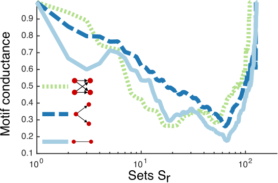
Figure S7: Sweep profile plot ($\phi_{M}(S)$ as a function of $S$ from the sweep in Algorithm 1) for $M_{\textnormal{bifan}}$ (green) $M_{8}$ (dark blue), and $M_{\textnormal{edge}}$ (light blue).

We found the motif-based clusters for motifs $M_{\textnormal{bifan}}$, $M_{8}$, and $M_{\textnormal{edge}}$ by running Algorithm 1 on the largest connected component of the motif adjacency matrix. Sweep profile plots ($\phi_{M}(S)$ as a function of $S$ from the sweep in Algorithm 1) are shown in Figure S7 and show that the size of the $M_{\textnormal{bifan}}$ returned by Algorithm 1 cluster is smaller than the clusters for $M_{8}$ and $M_{\textnormal{edge}}$. In fact, the motif-based clusters for $M_{8}$ and $M_{\textnormal{edge}}$ essentially bisect the graph, containing 63 of 127 and 64 of 131 nodes, respectively. Of the 63 nodes in the $M_{8}$-based cluster, only 2 are in the edge-based cluster, so these partitions give roughly the same information.

Next, we compare the clusters found by existing methods to the $M_{\textnormal{bifan}}$-based cluster found by Algorithm 1. We will show that existing methods do not find the same group of nodes. Let $S_{\textnormal{bifan}}$ be the $M_{\textnormal{bifan}}$-based cluster, which consists of 20 nodes. The nodes correspond to the following neurons: IL1DL/VL, IL2DL/DR/VL/VR/L/R, OLQDL/R, RIH, RIPL/R, RMEL/R/V, and URADL/DR/VL/VR. The partitions based on $M_{8}$ and $M_{\textnormal{edge}}$ provide two sets of nodes each. For the subsequent analysis, we consider the set with the largest number of overlapping nodes with $S_{\textnormal{bifan}}$. Call these sets $S_{M_{8}}$ and $S_{\textnormal{edge}}$. We also consider the cluster found by Infomap and the Louvain method with the largest overlap with $S_{\textnormal{bifan}}$. Call these sets $S_{I}$ and $S_{L}$.

To compare the most similar clusters found by other methods to $S_{\textnormal{bifan}}$, we look at two metrics. First, how many neurons in $S_{\textnormal{bifan}}$ are in a cluster found by existing methods (in other words, the overlap). A cluster consisting of all nodes in the graph would trivially have 100% overlap with $S_{\textnormal{bifan}}$ but loses all precision in the cluster identification. Thus, we also consider the sizes of the clusters. These metrics are summarized as follows:

$$\lvert S_{\textnormal{bifan}}\cap S_{M_{8}}\rvert=20, \lvert S_{M_{8}}\rvert=68$$

$$\lvert S_{\textnormal{bifan}}\cap S_{\textnormal{edge}}\rvert=20, \lvert S_{\textnormal{edge}}\rvert=64$$

$$\lvert S_{\textnormal{bifan}}\cap S_{L}\rvert=13, \lvert S_{L}\rvert=27$$

$$\lvert S_{\textnormal{bifan}}\cap S_{I}\rvert=19, \lvert S_{I}\rvert=114$$

We see that $S_{\textnormal{bifan}}$ is a subset of $S_{M_{8}}$ and $S_{\textnormal{edge}}$ and has substantial overlap with $S_{I}$. However, $S_{\textnormal{bifan}}$ is by far the smallest of all of these sets. We conclude that existing methods do not capture the same information as motif $M_{\textnormal{bifan}}$.

To further investigate the structure found by existing methods, we show the clusters $S_{\textnormal{edge}}$ and $S_{M_{8}}$ in Figure S8. From the figure, we see that spectral clustering based on edges or motif $M_{8}$ simply finds a spatially coherent cluster, rather than the control structure formed by the nodes in $S_{\textnormal{bifan}}$.

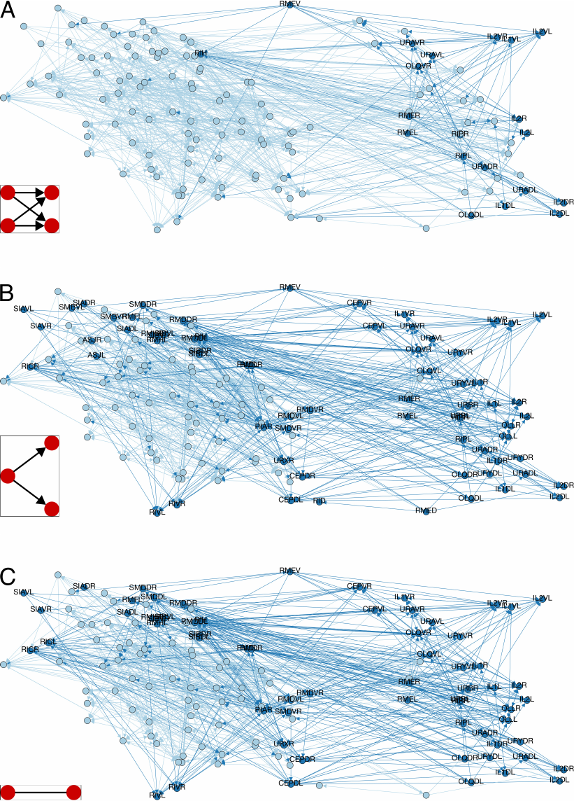
Figure S8: Illustration of motif-based clusters with true two-dimensional spatial dimensions of the frontal neurons of C. elegans. A: The $M_{\textnormal{bifan}}$-based cluster consists of the labeled dark blue nodes. B: Partitioning the graph based on motif $M_{8}$, where the labeled dark blue nodes are the nodes on the side of the partition with largest overlap of the nodes in A. C: Partitioning the graph based on edges, where the labeled dark blue nodes are the nodes on the side of the partition with largest overlap of the nodes in A. Note that the partitions in Figures B and C capture the cluster in Figure A, but also contain many other nodes. Essentially, the partitions in B and C are just capturing spatial information.

S6 Details and comparison against existing methods for the transportation reachability network

The nodes in the transportation reachability network are airports in the United States and Canada. There is an edge from city $i$ to city $j$ if the estimated travel time from $i$ to $j$ is less than some threshold  (?). The network is not symmetric. The network with estimated travel times was downloaded from
http://www.psi.toronto.edu/affinitypropagation/TravelRouting.mat and http://www.psi.toronto.edu/affinitypropagation/TravelRoutingCityNames.txt. We collected the latitude, longitude, and metropolitan populations of the cities using WolframAlpha and Wikipedia. All of the data is available on our project web page: http://snap.stanford.edu/higher-order/.

S6.1 Methods for spectral embeddings

We compared the motif-based spectral embedding of the transportation reachability network to spectral embeddings from other connectivity matrices. For this analysis, we ignore the travel times times and only consider the topology of the network. The two-dimensional spectral embedding for a graph defined by a (weighted) adjacency matrix $W\in\mathbb{R}^{n\times n}$ comes from Algorithm 2:

1. Form the normalized Laplacian $\mathcal{L}=I-D^{-1/2}WD^{-1/2}$, where $D$ is the diagonal degree matrix with $D_{ii}=\sum_{j}W_{ij}$.

2. Compute the first 3 eigenvectors $z_{1}$, $z_{2}$, $z_{3}$ of smallest eigenvalues for $\mathcal{L}$ ($z_{1}$ has the smallest eigenvalue).

3. Form the normalized matrix $Y\in\mathbb{R}^{n\times 3}$ by $Y_{ij}=z_{ij}/\sqrt{\sum_{j=1}^{3}z_{ij}^{2}}$.

4. Define the primary and secondary spectral coordinates of node $i$ to be $Y_{i2}$ and $Y_{i3}$, respectively.

We consider the following three matrices $W$.

1. Motif: The sum of the motif adjacency matrix (Equation S20) for three different anchored motifs:

   $$B_{1}=\begin{bmatrix}0&1&1\\ 1&0&1\\ 1&1&0\end{bmatrix},\;B_{2}=\begin{bmatrix}0&1&1\\ 1&0&1\\ 0&1&0\end{bmatrix},\;B_{3}=\begin{bmatrix}0&1&0\\ 1&0&1\\ 0&1&0\end{bmatrix},\;\mathcal{A}=\{1,3\}.$$ (S31)

   If $S$ is the matrix of bidirectional links in the graph ($S_{ij}=1$ if and only if $A_{ij}=A_{ji}=1$), then the motif adjacency matrix for these motifs is $W_{M}=S^{2}$. The resulting embedding is shown in Figure 4C of the main text.

2. Undirected: The adjacency matrix is formed by ignoring edge direction. This is the standard spectral embedding. The resulting embedding is shown in Figure 4D of the main text.

3. Undirected complement: The adjacency matrix is formed by taking the complement of the undirected adjacency matrix. This matrix tends to connect non-hubs to each other.

The networks represented by each adjacency matrices are all connected.

S6.2 Comparison of motif-based embedding to other embeddings

We computed 99% confidence intervals for the Pearson correlation of the primary spectral coordinate with the metropolitan population of the city using the Pearson correlation coefficient. Table S7 lists the confidence intervals. (Since eigenvectors are only unique up to sign, the confidence intervals are symmetric about $0$. We list the interval with the largest positive end point under this permutation to be consistent across embeddings.) The motif-based primary spectral coordinate has the strongest correlation with the city populations.

We repeated the computations for the correlation between the secondary spectral coordinate and the longitude of the city. Again, the motif-based clustering has the strongest correlation. Furthermore, the lower end of the confidence interval for the motif-based embedding was above the higher end of the confidence interval for the other three embeddings.

Table S7: Summary of Pearson correlations for spectral embeddings of the transportation reachability network. We list the 99% confidence interval for the Pearson correlation coefficient.

	Primary spectral coordinate	Secondary spectral coordinate
	and metropolitan population	and longitude
Embedding	99% confidence interval	99% confidence interval
Motif	0.43 $\pm$ 0.09	0.59 $\pm$ 0.08
Undirected	0.11 $\pm$ 0.12	0.39 $\pm$ 0.11
Undirected complement	0.31 $\pm$ 0.11	0.10 $\pm$ 0.12

Finally, in order to visualize these relationships, we computed Loess regressions of city metropolitan population and longitude against the primary and secondary spectral coordinates for each of the embeddings (Figure S9). The sign of the eigenvector used in each regression was chosen to match correlation shown in Figures 3C and 3D in the main text (primary spectral coordinate positively correlated with population and secondary spectral coordinate negatively correlated with longitude). The Loess regressions visualize the stronger correlation of the motif-based spectral coordinates with the metropolitan popuatlion and longitude.

We conclude that the embedding provided by the motif adjacency matrix more strongly captures the hub nature of airports and West-East geography of the network. To gain further insight into the relationship of the primary spectral coordinate’s relationship with the hub airports, we visualize the adjacency matrix in Figure S10, where the nodes are ordered by the spectral ordering. We see a clear relationship between the spectral ordering and the connectivity.

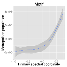
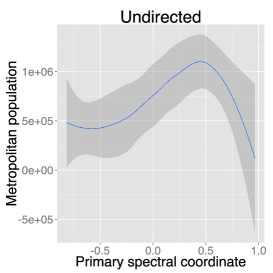
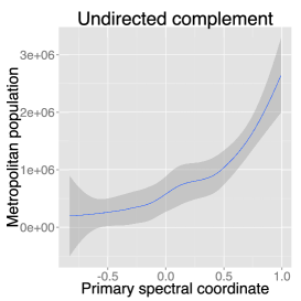
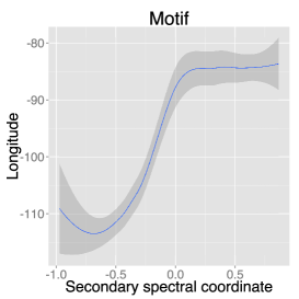
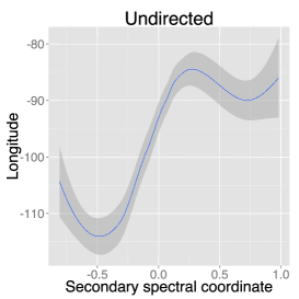
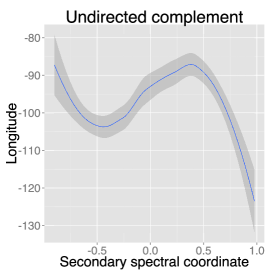
Figure S9: Loess regressions of city metropolitan population against the primary spectral coordinate (top) and longitude against secondary spectral coordinate (bottom) for the motif (left), undirected (middle), and undirected complement (right) adjacency matrices.

Figure S10: Visualization of transportation reachability network. Nodes are ordered by the spectral ordering provided by the motif adjacency matrix. A black dot means no edge exists in the network. For the edges in the network, lighter colors mean longer estimated travel times.

S7 Additional case studies

We next use motif-based clustering to analyze several additional networks. Our main goal is to show that motif-based clusters find markedly different structures in many real-world networks compared to edge-based clusters. For the case of a transcription regulation network of yeast, we also show that motif-based clustering more accurately finds known functional modules compared to existing methods. On the English Wikipedia article network and the Twitter network, we identify motifs that find anomalous clusters. On the Stanford web graph and in collaboration networks, we use motifs that have previously been studied in the literature and see how they reveal organizational structure in the networks.

S7.1 Motif $M_{6}$ in the Florida Bay food web

We now apply the higher-order clustering framework on the Florida Bay ecosystem food web  (?). The dataset was downloaded from http://vlado.fmf.uni-lj.si/pub/networks/data/bio/foodweb/Florida.paj. In this network, the nodes are compartments (roughly, organisms and species) and the edges represent directed carbon exchange (in many cases, this means that species $j$ eats species $i$). Motifs model energy flow patterns between several species.

S7.1.1 Identifying higher-order modular organization

In this case study, we use the framework to identify higher-order modular organization of networks. We focus on three motifs: $M_{5}$ corresponds to a hierarchical flow of energy where species $i$ and $j$ are energy sources (prey) for species $k$, and $i$ is also an energy source for $j$; $M_{6}$ models two species that prey on each other and then compete to feed on a common third species; and $M_{8}$ describes a single species serving as an energy source for two non-interacting species. Motif $M_{5}$ is considered a building block for food webs  (?, ?), and the prevalence of motif $M_{6}$ is predicted by a certain niche model  (?).

The framework reveals that low motif conductance (high-quality) clusters only exist for motif $M_{6}$ (motif conductance 0.12), whereas clusters based on motifs $M_{5}$ or $M_{8}$ have high motif conductance (see Figure S11). In fact, the motif Cheeger inequality (Theorem 6) guarantees that clustering based on motif $M_{5}$ or $M_{8}$ will always have larger motif conductance that clustering based on $M_{6}$. The inequality says that the motif conductance for any cluster in a connected motif adjacency matrix is at least half of the second smallest eigenvalue of the motif-normalized Laplacian. However, finding the cluster with optimal conductance is still computationally infeasible in general  (?).

The lower bounds using the largest connected component of the motif adjacency matrix for motifs $M_{5}$, $M_{6}$, and $M_{8}$ were 0.2195, 0.0335, and 0.2191, and the clusters found by the Algorithm 1 had motif conductances of 0.4414, 0.1200, and 0.4145. Thus, the cluster $S$ found by the algorithm for $M_{6}$ has smaller motif $M_{6}$-conductance (0.12) than any possible cluster’s motif-$M_{5}$ or motif-$M_{8}$ conductance. To state this formally, let $C$ be the cluster found by the algorithm for motif $M_{6}$ and let $H_{M}$ be the largest connected component of motif adjacency matrix for motif $M$. Then

$$\phi_{M_{6}}(H_{M_{6}},C)\leq\min\left\{\min_{S}\phi_{M_{5}}(H_{M_{5}},S),\;\min_{S}\phi_{M_{8}}(H_{M_{8}},S)\right\}.$$ (S32)

This means that, in terms of motif conductance, any cluster based on motifs $M_{5}$ or $M_{8}$ is worse than the cluser found by the algorithm in Theorem 6 for motif $M_{6}$. We note that the same conclusions hold for edge-based clustering. For motif $M_{\textnormal{edge}}$, the lower bound on conductance was 0.2194 and the cluster found by the algorithm had conductance 0.4083.

S7.1.2 Analysis of higher-order modular organization

Subsequently, we used motif $M_{6}$ to cluster the food web, revealing four clusters (Figure S11). Three represent well-known aquatic layers: (i) the pelagic system; (ii) the benthic predators of eels, toadfish, and crabs; (iii) the sea-floor ecosystem of macroinvertebrates. The fourth cluster identifies microfauna supported by particulate organic carbon in water and free bacteria. Table S7.1.3 lists the nodes in each cluster.

We also measured how well the motif-based clusters correlate to known ground truth system subgroup classifications of the nodes  (?). These classes are microbial, zooplankton, and sediment organism microfauna; detritus; pelagic, demersal, and benthic fishes; demseral, seagrass, and algae producers; and macroinvertebrates (Table S7.1.3). We also consider a set of labels which does not include the subclassification for microfauna and producers. In this case, the labels are microfauna; detritus; pelagic, demersal, and benthic fishes; producers; and macroinvertebrates.

To quantify how well the clusters found by motif-based clustering reflect the ground truth labels, we used several standard evaluation criteria: adjusted rand index, F1 score, normalized mutual information, and purity  (?). We compared these results to the clusters of several methods using the same evaluation criteria. In total, we evaluated six methods:

1. Motif-based clustering with the embedding + k-means algorithm (Algorithm 2) with 500 iterations of k-means.

2. Motif-based clustering with recursive bi-partitioning (repeated application of Algorithm 1 on the largest remaining compoennt). The process continues to cut the largest cluster until there are 4 total.

3. Edge-based clustering with the embedding + k-means algorithm, again with 500 iterations of k-means.

4. Edge-based clustering with recursive bi-partitioning with the same partitioning process.

5. The Infomap algorithm.

6. The Louvain method.

For the first four algorithms, we control the number of clusters, which we set to 4. For the last two algorithms, we cannot control the number of clusters. However, both methods found 4 clusters.

Table S7.1.3 shows that the motif-based clustering by embedding + k-means had the best performance for each classification criterion on both classifications. We conclude that the organization of compartments in the Florida Bay foodweb are better described motif $M_{6}$ than by edges.

S7.1.3 Connected components of the motif adjacency matrices

Finally, we discuss the discuss the preprocessing step of our method, where we compute computed connected components of the motif adjacency matrices. The original network has 128 nodes and 2106 edges. The largest connected component of the motif adjacency matrix for motif $M_{5}$ contains 127 of the 128 nodes. The node corresponding to the compartment of “roots” is the only node not in the largest connected component. The two largest connected components of the motif adjacency matrix for motif $M_{6}$ contain 12 and 50 nodes. The remaining 66 nodes are isolated. Table S7.1.3 lists the nodes in each component. We note that the group of 12 nodes corresponds to the green cluster in Figure S11. The motif adjacency matrix for $M_{8}$ is connected. The original network is weakly connected, so the motif adjacency matrix for $M_{\textnormal{edge}}$ is also connected.

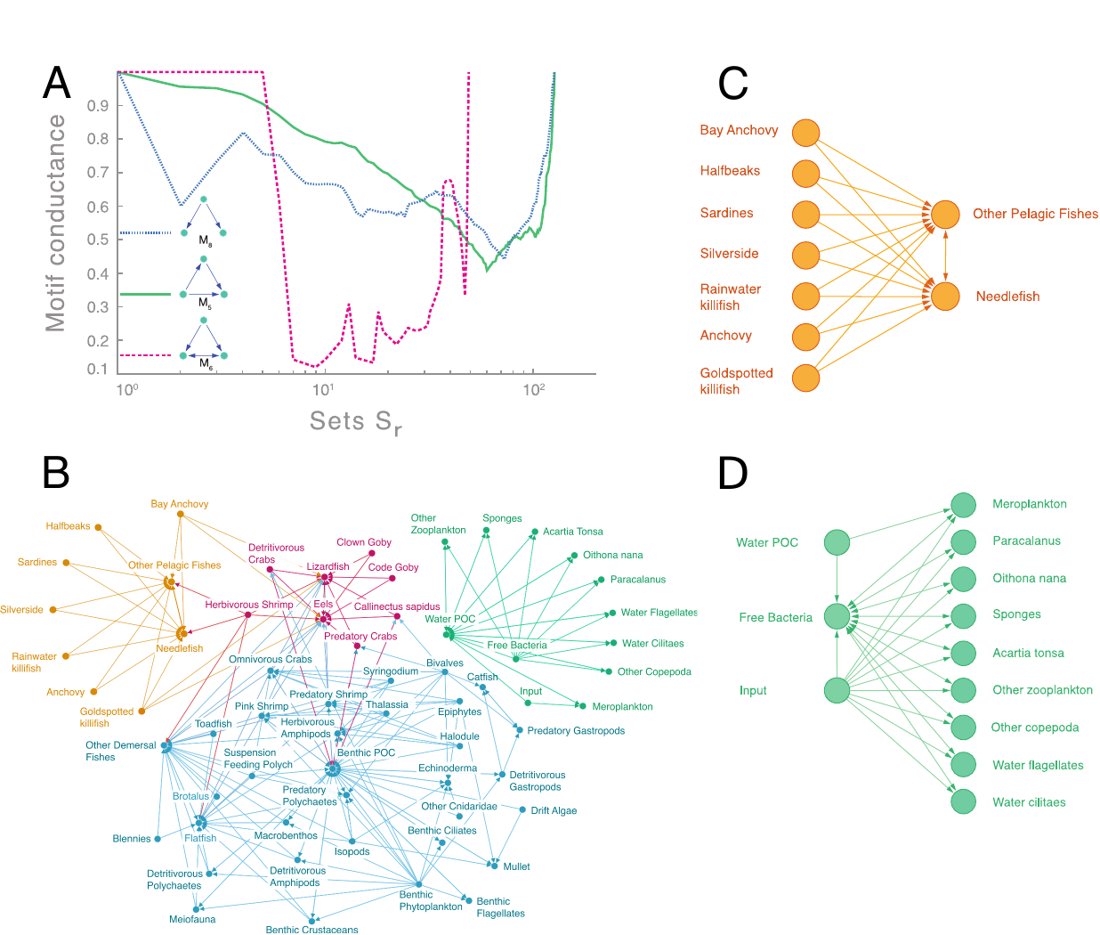
Figure S11: Higher-order organization of the Florida Bay food web. A: Sweep profile plot ($\phi^{(G)}_{M}(S)$ as a function of $S$ from the sweep in Algorithm 1) for different motifs on the Florida Bay ecosystem food web  (?). A priori it is not clear whether the network is organized based on a given motif. For example, motifs $M_{5}$ (green) and $M_{8}$ (blue) do not reveal any higher-order organization (motif conductance has high values). However, the downward spikes of the red curve show that $M_{6}$ reveals rich higher-order modular structure  (?). Ecologically, motif $M_{6}$ corresponds to two species mutually feeding on each other and also preying on a common third species. B: Clustering of the food web based on motif $M_{6}$. (For illustration, edges not participating in at least one instance of the motif are omitted.) The clustering reveals three known aquatic layers: pelagic fishes (yellow), benthic fishes and crabs (red), and sea-floor macroinvertebrates (blue) as well as a cluster of microfauna and detritus (green). Our framework identifies these modules with higher accuracy (61%) than existing methods (48–53%). C: A higher-order cluster (yellow nodes in (B)) shows how motif $M_{6}$ occurs in the pelagic layer. The needlefish and other pelagic fishes eat each other while several other fishes are prey for these two species. D: Another higher-order cluster (green nodes in (B)) shows how motif $M_{6}$ occurs between microorganisms. Here, several microfauna decompose into Particulate Organic Carbon in the water (water POC) but also consume water POC. Free bacteria serves as an energy source for both the microfauna and water POC.

Table S8: Connected components of the Florida Bay foodweb motif adjacency matrix for motif $M_{6}$. There are 50 nodes in component 1, 12 nodes in component 2, and 66 isolated nodes.

Two largest components		Isolated nodes
Compartment (node)	Component index	Compartment (node)
Benthic Phytoplankton	1	Barracuda
Thalassia	1	$2\text{\,}\mathrm{\SIUnitSymbolMicro m}$ Spherical Phytoplankt
Halodule	1	Synedococcus
Syringodium	1	Oscillatoria
Drift Algae	1	Small Diatoms ($<$$20\text{\,}\mathrm{\SIUnitSymbolMicro m}$)
Epiphytes	1	Big Diatoms ($>$$20\text{\,}\mathrm{\SIUnitSymbolMicro m}$)
Predatory Gastropods	1	Dinoflagellates
Detritivorous Polychaetes	1	Other Phytoplankton
Predatory Polychaetes	1	Roots
Suspension Feeding Polych	1	Coral
Macrobenthos	1	Epiphytic Gastropods
Benthic Crustaceans	1	Thor Floridanus
Detritivorous Amphipods	1	Lobster
Herbivorous Amphipods	1	Stone Crab
Isopods	1	Sharks
Herbivorous Shrimp	1	Rays
Predatory Shrimp	1	Tarpon
Pink Shrimp	1	Bonefish
Benthic Flagellates	1	Other Killifish
Benthic Ciliates	1	Snook
Meiofauna	1	Sailfin Molly
Other Cnidaridae	1	Hawksbill Turtle
Silverside	1	Dolphin
Echinoderma	1	Other Horsefish
Bivalves	1	Gulf Pipefish
Detritivorous Gastropods	1	Dwarf Seahorse
Detritivorous Crabs	1	Grouper
Omnivorous Crabs	1	Jacks
Predatory Crabs	1	Pompano
Callinectes sapidus (blue crab)	1	Other Snapper
Mullet	1	Gray Snapper
Blennies	1	Mojarra
Code Goby	1	Grunt
Clown Goby	1	Porgy
Flatfish	1	Pinfish
Sardines	1	Scianids
Anchovy	1	Spotted Seatrout
Bay Anchovy	1	Red Drum
Lizardfish	1	Spadefish
Catfish	1	Parrotfish
Eels	1	Mackerel
Toadfish	1	Filefishes
Brotalus	1	Puffer
Halfbeaks	1	Loon
Needlefish	1	Greeb
Goldspotted killifish	1	Pelican
Rainwater killifish	1	Comorant
Other Pelagic Fishes	1	Big Herons and Egrets
Other Demersal Fishes	1	Small Herons and Egrets
Benthic Particulate Organic Carbon (Benthic POC)	1	Ibis
Free Bacteria	2	Roseate Spoonbill
Water Flagellates	2	Herbivorous Ducks
Water Cilitaes	2	Omnivorous Ducks
Acartia Tonsa	2	Predatory Ducks
Oithona nana	2	Raptors
Paracalanus	2	Gruiformes
Other Copepoda	2	Small Shorebirds
Meroplankton	2	Gulls and Terns
Other Zooplankton	2	Kingfisher
Sponges	2	Crocodiles
Water Particulate Organic Carbon (Water POC)	2	Loggerhead Turtle
Input	2	Green Turtle
		Manatee
		Dissolved Organic Carbon (DOC)
		Output
		Respiration

Table S9: Ecological classification of nodes in the Florida Bay foodweb. Colors correspond to the colors in the clustering of Figure S11.

Compartment (node)	Classification 1	Classification 2	Assignment
Free Bacteria	Microbial microfauna	Microfauna	Green
Water Flagellates	Microbial microfauna	Microfauna	Green
Water Cilitaes	Microbial microfauna	Microfauna	Green
Acartia Tonsa	Zooplankton microfauna	Microfauna	Green
Oithona nana	Zooplankton microfauna	Microfauna	Green
Paracalanus	Zooplankton microfauna	Microfauna	Green
Other Copepoda	Zooplankton microfauna	Microfauna	Green
Meroplankton	Zooplankton microfauna	Microfauna	Green
Other Zooplankton	Zooplankton microfauna	Microfauna	Green
Sponges	Macroinvertebrates	Macroinvertebrates	Green
Water POC	Detritus	Detritus	Green
Input	Detritus	Detritus	Green
Sardines	Pelagic Fishes	Pelagic Fishes	Yellow
Anchovy	Pelagic Fishes	Pelagic Fishes	Yellow
Bay Anchovy	Pelagic Fishes	Pelagic Fishes	Yellow
Halfbeaks	Pelagic Fishes	Pelagic Fishes	Yellow
Needlefish	Pelagic Fishes	Pelagic Fishes	Yellow
Goldspotted killifish	Fishes Demersal	Fishes Demersal	Yellow
Rainwater killifish	Fishes Demersal	Fishes Demersal	Yellow
Silverside	Pelagic Fishes	Pelagic Fishes	Yellow
Other Pelagic Fishes	Pelagic Fishes	Pelagic Fishes	Yellow
Detritivorous Crabs	Macroinvertebrates	Macroinvertebrates	Red
Predatory Crabs	Macroinvertebrates	Macroinvertebrates	Red
Callinectus sapidus	Macroinvertebrates	Macroinvertebrates	Red
Lizardfish	Benthic Fishes	Benthic Fishes	Red
Eels	Fishes Demersal	Fishes Demersal	Red
Code Goby	Benthic Fishes	Benthic Fishes	Red
Clown Goby	Benthic Fishes	Benthic Fishes	Red
Herbivorous Shrimp	Macroinvertebrates	Macroinvertebrates	Red
Benthic Phytoplankton	Producer Demersal	Producer	Blue
Thalassia	Producer Seagrass	Producer	Blue
Halodule	Producer Seagrass	Producer	Blue
Syringodium	Producer Seagrass	Producer	Blue
Drift Algae	Producer Algae	Producer	Blue
Epiphytes	Producer Algae	Producer	Blue
Benthic Flagellates	Sediment Organism microfauna	Microfauna	Blue
Benthic Ciliates	Sediment Organism microfauna	Microfauna	Blue
Meiofauna	Sediment Organism microfauna	Microfauna	Blue
Other Cnidaridae	Macroinvertebrates	Macroinvertebrates	Blue
Echinoderma	Macroinvertebrates	Macroinvertebrates	Blue
Bivalves	Macroinvertebrates	Macroinvertebrates	Blue
Detritivorous Gastropods	Macroinvertebrates	Macroinvertebrates	Blue
Predatory Gastropods	Macroinvertebrates	Macroinvertebrates	Blue
Detritivorous Polychaetes	Macroinvertebrates	Macroinvertebrates	Blue
Predatory Polychaetes	Macroinvertebrates	Macroinvertebrates	Blue
Suspension Feeding Polych	Macroinvertebrates	Macroinvertebrates	Blue
Macrobenthos	Macroinvertebrates	Macroinvertebrates	Blue
Benthic Crustaceans	Macroinvertebrates	Macroinvertebrates	Blue
Detritivorous Amphipods	Macroinvertebrates	Macroinvertebrates	Blue
Herbivorous Amphipods	Macroinvertebrates	Macroinvertebrates	Blue
Isopods	Macroinvertebrates	Macroinvertebrates	Blue
Predatory Shrimp	Macroinvertebrates	Macroinvertebrates	Blue
Pink Shrimp	Macroinvertebrates	Macroinvertebrates	Blue
Omnivorous Crabs	Macroinvertebrates	Macroinvertebrates	Blue
Catfish	Benthic Fishes	Benthic Fishes	Blue
Mullet	Pelagic Fishes	Pelagic Fishes	Blue
Benthic POC	Detritus	Detritus	Blue
Toadfish	Benthic Fishes	Benthic Fishes	Blue
Brotalus	Fishes Demersal	Fishes Demersal	Blue
Blennies	Benthic Fishes	Benthic Fishes	Blue
Flatfish	Benthic Fishes	Benthic Fishes	Blue
Other Demersal Fishes	Fishes Demersal	Fishes Demersal	Blue

Table S10: Comparison of motif-based algorithms against other methods in finding ground truth structure in the Florida Bay food web  (?). Performance for identifying the two classifications provided in Table S7.1.3 was evaluated based on Adjusted Rand Index (ARI), F1 score, Normalized Mutual Information (NMI), and Purity. In all cases, the motif-based methods have the best performance.

	Evaluation	Motif embedding	Motif recursive	Edge embedding	Edge recursive	XXInfomapXX	Louvain
		+ k-means	bi-partitioning	+ k-means	bi-partitioning
Classification 1	ARI	0.3005	0.2156	0.1564	0.1226	0.1423	0.2207
	F1	0.4437	0.3853	0.3180	0.2888	0.3100	0.4068
	NMI	0.5040	0.4468	0.4112	0.3879	0.4035	0.4220
	Purity	0.5645	0.5323	0.4032	0.4194	0.4194	0.5323
Classification 2	ARI	0.3265	0.2356	0.1814	0.1190	0.1592	0.2207
	F1	0.4802	0.4214	0.3550	0.3035	0.3416	0.4068
	NMI	0.4822	0.4185	0.3533	0.3034	0.3471	0.4220
	Purity	0.6129	0.5806	0.4839	0.4355	0.4677	0.5323

S7.2 Coherent feedforward loops in the S. cerevisiae transcriptional regulation network

In this network, each node is an operon (a group of genes in a mRNA molecule), and a directed edge from operon $i$ to operon $j$ means that $i$ is regulated by a transcriptional factor encoded by $j$  (?). Edges are directed and signed. A positive sign represents activation and a negative sign represents repression. The network data was downloaded from http://www.weizmann.ac.il/mcb/UriAlon/sites/mcb.UriAlon/files/uploads/NMpaper/yeastdata.mat and http://www.weizmann.ac.il/mcb/UriAlon/sites/mcb.UriAlon/files/uploads/DownloadableData/list_of_ffls.pdf.

For this case study, we examine the coherent feedforward loop motif (see Figure S12), which act as sign-sensitive delay elements in transcriptional regulation networks  (?, ?). Formally, the feedforward loop is represented by the following signed motifs

$$B_{1}=\begin{bmatrix}0&+&+\\ 0&0&+\\ 0&0&0\end{bmatrix},\;B_{2}=\begin{bmatrix}0&-&-\\ 0&0&+\\ 0&0&0\end{bmatrix},\;B_{3}=\begin{bmatrix}0&+&-\\ 0&0&-\\ 0&0&0\end{bmatrix},\;B_{4}=\begin{bmatrix}0&-&+\\ 0&0&-\\ 0&0&0\end{bmatrix}.$$ (S33)

These motifs have the same edge pattern and only differ in sign. All of the motifs are simple ($\mathcal{A}=\{1,2,3\}$). For our analysis, we consider all coherent feedforward loops that are subgraphs on the induced subgraph of any three nodes. However, there is only one instance where the coherent feedforward loop itself is a subgraph but not an induced subgraph on three nodes. Specifically, the induced subgraph by DAL80, GAT1, and GLN3 contains a bi-directional edge between DAL80 and GAT1, unidirectional edges from DAL80 and GAT1 to GLN3.

S7.2.1 Connected components of the adjacency matrices

Table S11: Connected components of size greater than one for the motif adjacency matrix in the S. cerevisiae network for the coherent feedforward loop.

Size	operons
18	ALPHA1, CLN1, CLN2, GAL11, HO, MCM1, MFALPHA1, PHO5, SIN3,
	SPT16, STA1, STA2, STE3, STE6, SWI1, SWI4/SWI6, TUP1, SNF2/SWI1
9	HXT11, HXT9, IPT1, PDR1, PDR3, PDR5, SNQ2, YOR1, YRR1
9	GCN4, ILV1, ILV2, ILV5, LEU3, LEU4, MET16, MET17, MET4
6	CHO1, CHO2, INO2, INO2/INO4, OPI3, UME6
6	DAL80, DAL80/GZF3, GAP1, GAT1, GLN1, GLN3
5	CYC1, GAL1, GAL4, MIG1, HAP2/3/4/5
3	ADH2, CCR4, SPT6
3	CDC19, RAP1, REB1
3	DIT1, IME1, RIM101

Again, we analyze the component structure of the motif adjacency matrix as a pre-processing step. The original network consists of 690 nodes and 1082 edges, and its largest weakly connected component consists of 664 nodes and 1066 edges. Every coherent feedforward loop in the network resides in the largest weakly connected component, so we subsequently consider this sub-network in the following analysis. Of the 664 nodes in the network, only 62 participate in a coherent feedforward loop. Forming the motif adjacency matrix results in nine connected components, of sizes 18, 9, 9, 6, 6, 5, 3, 3, and 3. The operons for the connected components consisting of more than one node is listed in Table S11.

S7.2.2 Comparison against existing methods

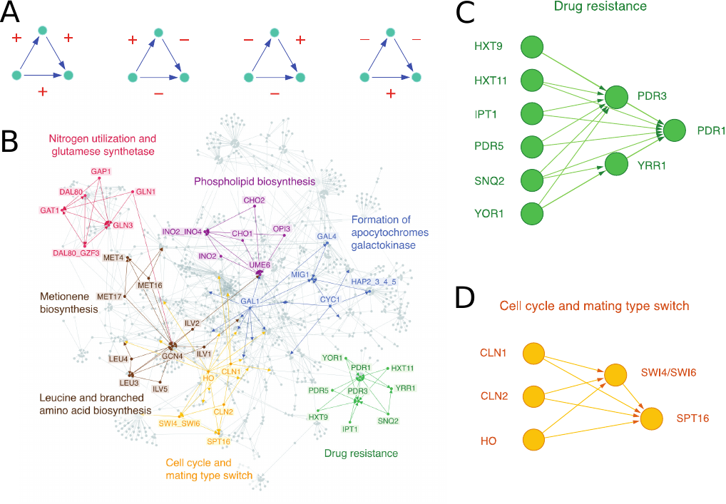
Figure S12: Higher-order organization of the S. cerevisiae transcriptional regulation network. A: The four higher-order structures used by our higher-order clustering method, which can model signed motifs. These are coherent feedfoward loop motifs, which act as sign-sensitive delay elements in transcriptional regulation networks  (?). The edge signs refer to activation (positive) or repression (negative). B: Six higher-order clusters revealed by the motifs in (A). Clusters show functional modules consisting of several motifs (coherent feedforward loops), which were previously studied individually  (?). The higher-order clustering framework identifies the functional modules with higher accuracy (97%) than existing methods (68–82%). C–D: Two higher-order clusters from (B). In these clusters, all edges have positive sign. The functionality of the motifs in the modules correspond to drug resistance (C) or cell cycle and mating type match (D). The clustering suggests that coherent feedforward loops function together as a single processing unit rather than as independent elements.

We note that, although the original network is connected, the motif adjacency matrix corresponds to a disconnected graph. This already reveals much of the structure in the network (Figure S12). Indeed, this “shattering” of the graph into components for the feedforward loop has previously been observed in transcriptional regulation networks  (?). We additionally used Algorithm 1 to partition the largest connected component of the motif adjacency matrix (consisting of 18 nodes). This revealed the cluster $\{$CLN2, CLN1, SWI4/SWI6, SPT16, HO$\}$, which contains three coherent feedforward loops (Figure S12). All three instances of the motif correspond to the function “cell cycle and mating type switch”. The motifs in this cluster are the only feedforward loops for which the function is described in Reference  (?). Using the same procedure on the undirected version of the induced subgraph of the 18 nodes (i.e., using motif $M_{\textnormal{edge}}$) results in the cluster $\{$CLN1, CLN2, SPT16, SWI4/SWI6 $\}$. This cluster breaks the coherent feedforward loop formed by HO, SWI4/SWI6, and SPT16.

We also evaluated our method based on the classification of motif functionality  (?). In total, there are 12 different functionalities and 29 instances of labeled coherent feedforward loops. We considered the motif-based clustering of the graph to be the connected components of the motif adjacency matrix with the additional partition of the largest connected component. To form an edge-based clustering, we used the embedding + k-means algorithm on the undirected graph (i.e., motif $M_{\textnormal{edge}}$) with $k=12$ clusters. We also clustered the graph using Infomap and the Louvain method. Table S7.2.2 summarizes the results. We see that the motif-based clustering coherently labels all 29 motifs in the sense that the three nodes in every instance of a labeled motif is placed in the same cluster. The edge-based spectral, Infomap, and Louvain clustering coherently labeled 25, 23, and 23 motifs, respectively.

We measured the accuracy of each clustering method as the rand index  (?) on the coherently labeled motifs, multiplied by the fraction of coherently labeled motifs. The motif-based clustering had the highest accuracy. We conclude that motif-based clustering provides an advantage over edge-based clustering methods in identifying functionalities of coherent feedforward loops in the the S. cerevisiae transcriptional regulation network.

Table S12: Classification of coherent feedforward loop motifs by several clustering methods. In a given motif instance, we say that it is coherently labeled if the nodes comprising the motif are in the same cluster. If a motif is not coherently labeled, a “-1” is listed. The accuracy is the rand index on the labels and motif functionality on coherently labeled motifs, multiplied by the fraction of coherently labeled motifs.

	Motif nodes			Function	Class label
					Motif-based	Edge-based	Infomap	Louvain
	GAL11	ALPHA1	MFALPHA1	pheromone response	1	1	-1	-1
	GCN4	MET4	MET16	Metionine biosynthesis	2	2	1	-1
	GCN4	MET4	MET17	Metionine biosynthesis	2	2	1	-1
	GCN4	LEU3	ILV1	Leucine and branched amino acid biosynthesis	2	2	1	1
	GCN4	LEU3	ILV2	Leucine and branched amino acid biosynthesis	2	2	1	1
	GCN4	LEU3	ILV5	Leucine and branched amino acid biosynthesis	2	2	1	1
	GCN4	LEU3	LEU4	Leucine and branched amino acid biosynthesis	2	2	1	1
	GLN3	GAT1	GAP1	Nitrogen utilization	3	3	1	2
	GLN3	GAT1	DAL80	Nitrogen utilization	3	3	1	2
	GLN3	GAT1	DAL80/GZF3	Glutamate synthetase	3	3	1	2
	GLN3	GAT1	GLN1	Glutamate synthetase	3	3	1	2
	MIG1	HAP2/3/4/5	CYC1	formation of apocytochromes	4	4	-1	-1
	MIG1	GAL4	GAL1	Galactokinase	4	-1	-1	-1
	PDR1	YRR1	SNQ2	Drug resistance	5	5	2	3
	PDR1	YRR1	YOR1	Drug resistance	5	5	2	3
	PDR1	PDR3	HXT11	Drug resistance	5	5	2	3
	PDR1	PDR3	HXT9	Drug resistance	5	5	2	3
	PDR1	PDR3	PDR5	Drug resistance	5	5	2	3
	PDR1	PDR3	IPT1	Drug resistance	5	5	2	3
	PDR1	PDR3	SNQ2	Drug resistance	5	5	2	3
	PDR1	PDR3	YOR1	Drug resistance	5	5	2	3
	RIM101	IME1	DIT1	sporulation-specific	6	6	3	4
	SPT16	SWI4/SWI6	CLN1	Cell cycle and mating type switch	7	-1	4	5
	SPT16	SWI4/SWI6	CLN2	Cell cycle and mating type switch	7	-1	-1	5
	SPT16	SWI4/SWI6	HO	Cell cycle and mating type switch	7	-1	-1	-1
	TUP1	ALPHA1	MFALPHA1	Mating factor alpha	1	1	-1	5
	UME6	INO2/INO4	CHO1	Phospholipid biosynthesis	8	6	5	4
	UME6	INO2/INO4	CHO2	Phospholipid biosynthesis	8	6	5	4
	UME6	INO2/INO4	OPI3	Phospholipid biosynthesis	8	6	5	4
Frac. coherently labeled					29 / 29	25 / 29	23 / 29	23 / 29
Accuracy					0.97	0.82	0.68	0.76

S7.3 Motif $M_{6}$ in the English Wikipedia article network

The English Wikipedia network  (?, ?, ?) consists of 4.21 million nodes (representing articles) and 101.31 million edges, where an edge from node $i$ to node $j$ means that there is a hyperlink from the $i$th article to the $j$th article. The network data was downloaded from http://law.di.unimi.it/webdata/enwiki-2013/.

We used Algorithm 1 to find a motif-based cluster for motif $M_{6}$ and $M_{\textnormal{edge}}$ (the algorithm was run on the largest connected component of the motif adjacency matrix). The clusters are shown in Figure S13. The nodes in the motif-based cluster are cities and barangays (small administrative divisions) in the Philippines. The cluster has a set of nodes with many outgoing links that form the source node in motif $M_{6}$. In total, the cluster consists of 22 nodes and 338 edges. The linking pattern appears anomalous and suggests that perhaps the pages uplinking should receive reciprocated links. On the other hand, the edge-based cluster is much larger cluster and does not have too much structure. The cluster consists of several high-degree nodes and their neighbors.

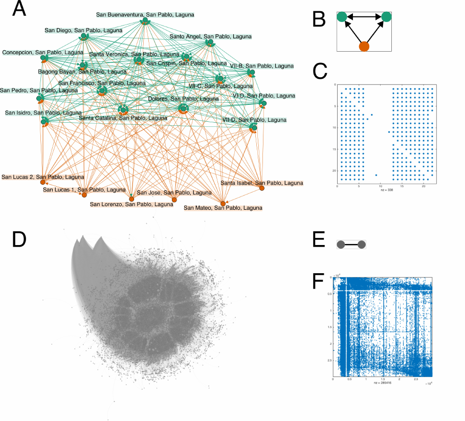
Figure S13: Clusters from the English Wikipedia hyperlink network  (?, ?, ?). A–C: Motif-based cluster (A) for motif $M_{6}$ (B). The cluster consists of cities and small administrative divisions in the Philippines. The green nodes have many bi-direction links with each other and many incoming links from orange nodes at the bottom of the figure. The spy plot illustrates this network structure (C). D–F: Cluster (D) for undirected edges (E). The cluster has a few very high-degree nodes, as evidenced by the spy plot (F).

S7.4 Motif $M_{6}$ in the Twitter follower network

We also analyzed the complete 2010 Twitter follower graph  (?, ?, ?). The graph consists 41.65 million nodes (users) and 1.47 billion edges, where an edge from node $i$ to node $j$ signifies that user $i$ is followed by user $j$ on the social network. The network data was downloaded from http://law.di.unimi.it/webdata/twitter-2010/.

We used Algorithm 1 to find a motif-based cluster for motif $M_{6}$ (the algorithm was run on the largest connected component of the motif adjacency matrix). The cluster contains 151 nodes and consists of two disconnected components. Here, we consider the smaller of the two components, which consists of 38 nodes. We also found an edge-based cluster on the undirected graph (using Algorithm 1 with motif $M_{\textnormal{edge}}$). This cluster consists of 44 nodes.

Figure S14 illustrates the motif-based and edge-based clusters. Both clusters capture anomalies in the graph. The motif-based cluster consists of holding accounts for a photography company. The nodes that form bi-directional links have completed profiles (contain a profile picture) while several nodes with incomplete profiles (without a profile picture) are followed by the completed accounts. The edge-based cluster is a near clique, where the user screen names all begin with “LC_”. We suspect that the similar usernames are either true social communities, holding accounts, or bots. (For the most part, their tweets are protected, so we could not verify if any of these scenarios are true). Interestingly, both $M_{6}$ and $M_{\textnormal{edge}}$ find anomalous clusters. However, their structures are quite different. We conclude that $M_{6}$ can lead to the detection of new anomalous clusters in social networks.

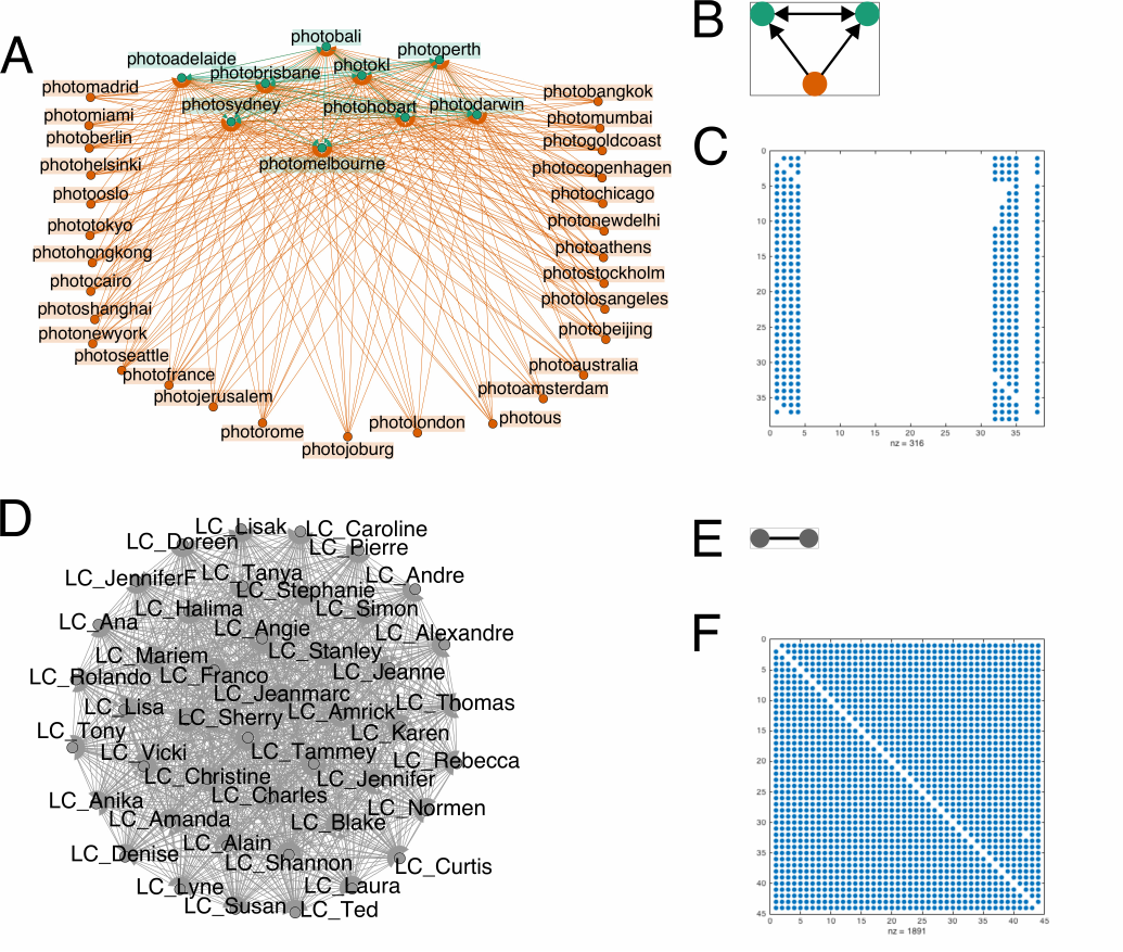
Figure S14: Clusters in the 2010 Twitter follower network  (?, ?, ?). A–C: Motif-based cluster (A) for motif $M_{6}$ (B). All accounts are holding accounts for a photography company. The green nodes correspond to accounts that have completed profiles, while the orange accounts have incomplete profiles. The spy plot illustrates how the cluster is formed around this motif (C). D–F: Cluster (D) for edge-based clustering (E). The cluster consists of a near-clique (F) where all users have the prefix “LC_”.

S7.5 Motif $M_{7}$ in the Stanford web graph

The Stanford web graph  (?, ?) consists of 281,903 nodes and 2,312,497 edges, where an edge from node $i$ to node $j$ means that there is a hyperlink from the $i$th web page to the $j$th web page. Here, all of the web pages come from the Stanford domain. The network data was downloaded from http://snap.stanford.edu/data/web-Stanford.html.

We used Algorithm 1 to find a motif-based cluster for motif $M_{7}$, a motif that is over-expressed in web graphs  (?). An illustration of the cluster and an edge-based cluster (i.e., using Algorithm 1 with $M_{\textnormal{edge}}$) are in Figure S15. Interestingly, both clusters exhibits a core-periphery structure, albeit markedly different ones. The motif-based cluster contains several core nodes with large in-degree. Such core nodes comprise the sink node in motif $M_{7}$. On the periphery are several clusters within which are many bi-directional links (as illustrated by the spy plot in Figure S15). The nodes in these clusters then up-link to the core nodes. This type of organizational unit suggests an explanation for why motif $M_{7}$ is over-expressed: clusters of similar pages tend to uplink to more central pages. The edge-based cluster also has a few nodes with large in-degree, serving as a small core. On the periphery are the neighbors of these nodes, which themselves tend not to be connected (as illustrated by the spy plot).

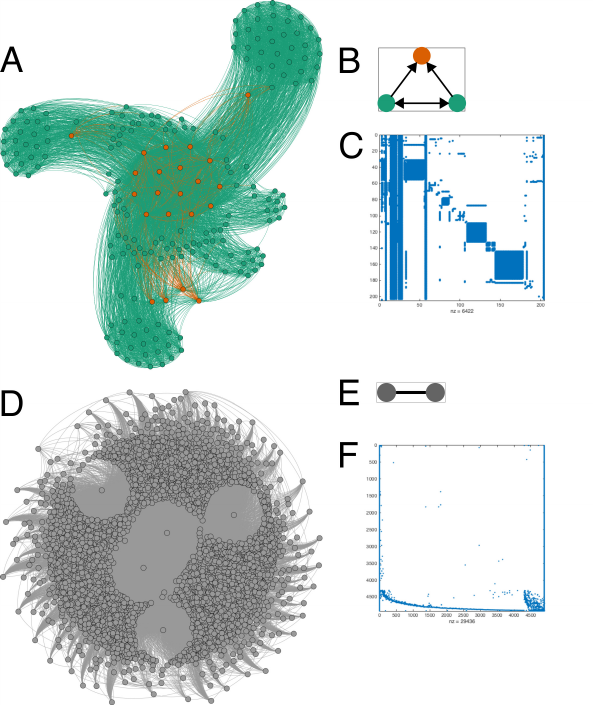
Figure S15: Clusters in the Stanford web graph  (?). A–C: Motif-based cluster (A) for motif $M_{7}$ (B). The cluster has a core group of nodes with many incoming links (serving as the sink node in $M_{7}$; shown in orange) and several periphery groups that are tied together (the bi-directional link in $M_{7}$; shown in green) and also up-link to the core. This is evident from the spy plot (C). D–F: Cluster (C) for undirected edges (B). The cluster contains a few high-degree nodes and their neighbors, and the neighbors tend to not be connected, as illustrated by the splot (F).

S7.6 Semi-cliques in collaboration networks

We used Algorithm 1 to identify clusters of a four-node motif (the semi-clique) that has been studied in conjunction with researcher productivity in collaboration networks  (?) (see Figure S16). We found a motif-based cluster in two different collaboration networks. Each one is derived from co-authorship in papers submitted to the arXiv under a certain category; here, we analyze the ”High Energy Physics–Theory” (HepTh) and ”Condensed Matter Physics” (CondMat) categories  (?, ?). The HepTh network has 23,133 nodes and 93,497 edges and the CondMat network has 9,877 nodes and 25,998 edges. The HepTh network data was downloaded from http://snap.stanford.edu/data/ca-HepTh.html and the CondMat network data was downloaded from http://snap.stanford.edu/data/ca-CondMat.html.

Figure S16 shows the two clusters for each of the collaboration networks. In both networks, the motif-based cluster consists of a core group of nodes and similarly-sized groups on the periphery. The core group of nodes correspond to the nodes of degree 3 in the motif and the periphery group nodes correspond to the nodes of degree 2. One explanation for this organization is that there is a small small group of authors that writes papers with different research groups. Alternatively, the co-authorship could come from a single research group, where senior authors are included on all of the papers and junior authors on a subset of the papers.

On the other hand, the edge-based clusters (i.e., result of Algorithm 1 for $M_{\textnormal{edge}}$) are a clique in the HepTh netowork and a clique with a few dangling nodes in the CondMat network. The dense clusters are quite different from the sparser clusters based on the semi-clique. Such dense clusters are not that surprising. For example, a clique could arise from a single paper published by a group of authors.

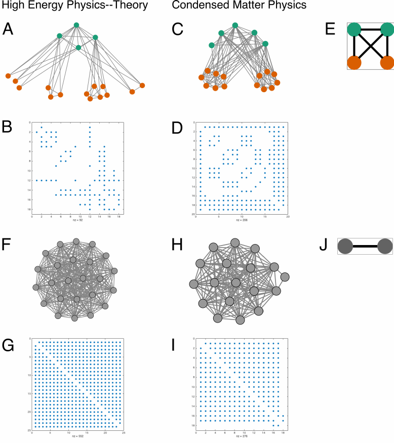
Figure S16: Clusters in co-authorship networks  (?). A–E: Best motif-based cluster for the semi-clique motif (E) in the High Energy Physics–Theory collaboration network (A) and the Condensed Matter Physics collaboration network (C). Corresponding spy plots are shown in (B) and (D). F–I: Best edge-based (I) cluster in the High Energy Physics–Theory collaboration network (F) and the Condensed Matter Physics collaboration network (H). Corresponding spy plots are shown in (G) and (I).

S8 Data availability

All data is available at our project web site at http://snap.stanford.edu/higher-order/. The web site includes links to datasets used for experiments throughout the supplementary material  (?, ?, ?, ?, ?, ?, ?, ?, ?, ?, ?, ?, ?, ?, ?).

Authors would like to thank Rok Sosič for insightful comments. ARB acknowledges the support of a Stanford Graduate Fellowship. DFG acknowledges the support of NSF CCF-1149756 and IIS-1422918 and DARPA SIMPLEX. JL acknowledges the support of NSF IIS-1149837 and CNS-1010921, NIH BD2K, DARPA XDATA and SIMPLEX, Boeing, Lightspeed, and Volkswagen.

References and Notes

- 1. R. Milo, et al., Science 298, 824 (2002).
- 2. S. Mangan, A. Zaslaver, U. Alon, Journal of molecular biology 334, 197 (2003).
- 3. J. Yang, J. Leskovec, Proceedings of the IEEE 102, 1892 (2014).
- 4. P. W. Holland, S. Leinhardt, American Journal of Sociology pp. 492–513 (1970).
- 5. M. Rosvall, A. V. Esquivel, A. Lancichinetti, J. D. West, R. Lambiotte, Nature communications 5 (2014).
- 6. N. Pržulj, D. G. Corneil, I. Jurisica, Bioinformatics 20, 3508 (2004).
- 7. J. Leskovec, K. J. Lang, A. Dasgupta, M. W. Mahoney, Internet Mathematics 6, 29 (2009).
- 8. Ö. N. Yaveroğlu, et al., Scientific reports 4 (2014).
- 9. S. Mangan, U. Alon, Proceedings of the National Academy of Sciences 100, 11980 (2003).
- 10. C. J. Honey, R. Kötter, M. Breakspear, O. Sporns, Proceedings of the National Academy of Sciences 104, 10240 (2007).
- 11. S. E. Schaeffer, Computer Science Review 1, 27 (2007).
- 12. Minimizing is NP-hard, which follows from the NP-hardness of the traditional definition of conductance (?).
- 13. See the Supplementary Material.
- 14. Formally, when the motif has three nodes, the selected cluster satisfies , where is the smallest motif conductance of any possible node set . This inequality is proved in the Supplementary Material.
- 15. The normalized motif Laplacian matrix is , where is a diagonal matrix with the row-sums of on the diagonal (), and is the same matrix with the inverse square-roots on the diagonal (). The spectral ordering is the by-value ordering of , where is the eigenvector corresponding to the second smallest eigenvalue of , i.e., is the index of with the th smallest value.
- 16. C. Seshadhri, A. Pinar, T. G. Kolda, Statistical Analysis and Data Mining: The ASA Data Science Journal 7, 294 (2014).
- 17. R. Andersen, F. Chung, K. Lang, Proceedings of the 47th Annual IEEE Symposium on Foundations of Computer Science (2006), pp. 475–486.
- 18. J. J. Whang, I. S. Dhillon, D. F. Gleich, SIAM Data Mining (2015).
- 19. A. Y. Ng, M. I. Jordan, Y. Weiss, Advances in Neural Information Processing Systems 14 (2002), pp. 849–856.
- 20. D. Boley, Data Mining and Knowledge Discovery 2, 325 (1998).
- 21. D. L. Riddle, T. Blumenthal, B. J. Meyer, et al., eds., C. elegans II (Cold Spring Harbor Laboratory Press, 1997), second edn.
- 22. H. Lee, et al., Nature neuroscience 15, 107 (2012).
- 23. B. J. Frey, D. Dueck, Science 315, 972 (2007).
- 24. B. Serrour, A. Arenas, S. Gómez, Computer Communications 34, 629 (2011).
- 25. T. Michoel, A. Joshi, B. Nachtergaele, Y. Van de Peer, Molecular BioSystems 7, 2769 (2011).
- 26. A. R. Benson, D. F. Gleich, J. Leskovec, SIAM Data Mining (2015).
- 27. F. Krzakala, et al., Proceedings of the National Academy of Sciences 110, 20935 (2013).
- 28. M. Kaiser, C. C. Hilgetag, PLoS Computational Biology 2, e95 (2006).
- 29. U. Alon, Nature Reviews Genetics 8, 450 (2007).
- 30. O. Sporns, R. Kötter, PLoS Biology 2, e369 (2004).
- 31. A. Inokuchi, T. Washio, H. Motoda, Principles of Data Mining and Knowledge Discovery (Springer, 2000), pp. 13–23.
- 32. F. R. Chung, Proceedings of ICCM (Citeseer, 2007), vol. 2, p. 378.
- 33. J. R. Lee, S. O. Gharan, L. Trevisan, Journal of the ACM 61, 37 (2014).
- 34. F. Chung, Annals of Combinatorics 9, 1 (2005).
- 35. D. Boley, G. Ranjan, Z.-L. Zhang, Linear Algebra and its Applications 435, 224 (2011).
- 36. F. D. Malliaros, M. Vazirgiannis, Physics Reports 533, 95 (2013).
- 37. G. Karypis, R. Aggarwal, V. Kumar, S. Shekhar, Very Large Scale Integration (VLSI) Systems, IEEE Transactions on 7, 69 (1999).
- 38. S. Agarwal, K. Branson, S. Belongie, Proceedings of the 23rd International Conference on Machine Learning (ACM, 2006), pp. 17–24.
- 39. D. Zhou, J. Huang, B. Schölkopf, Advances in Neural Information Processing Systems 19 (MIT Press, 2006), pp. 1601–1608.
- 40. J. Rodríguez, Linear and Multilinear Algebra 50, 1 (2002).
- 41. L. Trevisan, Lecture notes on expansion, sparsest cut, and spectral graph theory, http://www.eecs.berkeley.edu/~luca/books/expanders.pdf. Accessed June 28, 2015.
- 42. S. Demeyer, et al., PloS ONE 8, e61183 (2013).
- 43. M. Houbraken, et al., PLoS ONE 9, e97896 (2014).
- 44. S. Wernicke, IEEE/ACM Transactions on Computational Biology and Bioinformatics 3, 347 (2006).
- 45. S. Wernicke, F. Rasche, Bioinformatics 22, 1152 (2006).
- 46. C. R. Aberger, A. Nötzli, K. Olukotun, C. Ré, arXiv preprint arXiv:1503.02368 (2015).
- 47. M. Latapy, Theoretical Computer Science 407, 458 (2008).
- 48. J. W. Berry, et al., Proceedings of the 5th Conference on Innovations in Theoretical Computer Science (ACM, New York, NY, USA, 2014), pp. 225–234.
- 49. D. Marcus, Y. Shavitt, IEEE 30th International Conference on Distributed Computing Systems Workshops (2010), pp. 92–98.
- 50. N. Chiba, T. Nishizeki, SIAM Journal on Computing 14, 210 (1985).
- 51. T. Schank, D. Wagner, Experimental and Efficient Algorithms (Springer, 2005), pp. 606–609.
- 52. L. Becchetti, P. Boldi, C. Castillo, A. Gionis, Proceedings of the 14th ACM SIGKDD international conference on Knowledge discovery and data mining (ACM, 2008), pp. 16–24.
- 53. J. Cohen, Computing in Science & Engineering 11, 29 (2009).
- 54. B. N. Parlett, The Symmetric Eigenvalue Problem, vol. 7 (SIAM, 1980).
- 55. K. J. Maschhoff, D. C. Sorensen, Applied Parallel Computing Industrial Computation and Optimization (Springer, 1996), pp. 478–486.
- 56. J. Leskovec, A. Krevl, SNAP Datasets: Stanford large network dataset collection, http://snap.stanford.edu/data (2014).
- 57. P. Boldi, B. Codenotti, M. Santini, S. Vigna, Software: Practice and Experience 34, 711 (2004).
- 58. P. Boldi, S. Vigna, Proceedings of the 13th International Conference on World Wide Web (ACM, 2004), pp. 595–602.
- 59. P. Boldi, M. Rosa, M. Santini, S. Vigna, Proceedings of the 20th International Conference on World Wide Web (ACM, 2011), pp. 587–596.
- 60. P. Boldi, A. Marino, M. Santini, S. Vigna, Proceedings of the companion publication of the 23rd international conference on World wide web companion (International World Wide Web Conferences Steering Committee, 2014), pp. 227–228.
- 61. A. Azad, A. Buluç, J. R. Gilbert, Proceedings of the IPDPSW, Workshop on Graph Algorithm Building Blocks (GABB) (2015), pp. 804–811.
- 62. M. Rosvall, C. T. Bergstrom, Proceedings of the National Academy of Sciences 105, 1118 (2008).
- 63. V. D. Blondel, J.-L. Guillaume, R. Lambiotte, E. Lefebvre, Journal of statistical mechanics: theory and experiment 2008, P10008 (2008).
- 64. R. E. Ulanowicz, C. Bondavalli, M. S. Egnotovich, Trophic Dynamics in South Florida Ecosystem, FY 97: The Florida Bay Ecosystem, Tech. Rep. CBL 98-123, Chesapeake Biological Laboratory, Solomons, MD (1998).
- 65. J. Bascompte, C. J. Melián, E. Sala, Proceedings of the National Academy of Sciences of the United States of America 102, 5443 (2005).
- 66. J. Bascompte, et al., Science 325, 416 (2009).
- 67. D. B. Stouffer, J. Camacho, W. Jiang, L. A. N. Amaral, Proceedings of the Royal Society of London B: Biological Sciences 274, 1931 (2007).
- 68. D. Wagner, F. Wagner, Proceedings of the 18th International Symposium on Mathematical Foundations of Computer Science (1993), pp. 744–750.
- 69. C. D. Manning, P. Raghavan, H. Schütze, et al., Introduction to Information Retrieval, vol. 1 (Cambridge university press Cambridge, 2008).
- 70. R. Dobrin, Q. K. Beg, A.-L. Barabási, Z. N. Oltvai, BMC bioinformatics 5, 10 (2004).
- 71. H. Kwak, C. Lee, H. Park, S. Moon, Proceedings of the 19th International Conference on World Wide Web (ACM, 2010), pp. 591–600.
- 72. T. Chakraborty, N. Ganguly, A. Mukherjee, Advances in Social Networks Analysis and Mining (ASONAM), 2014 IEEE/ACM International Conference on (IEEE, 2014), pp. 130–137.
- 73. J. Leskovec, J. Kleinberg, C. Faloutsos, ACM Transactions on Knowledge Discovery from Data (TKDD) 1, 2 (2007).
- 74. R. West, H. S. Paskov, J. Leskovec, C. Potts, Transactions of the Association for Computational Linguistics 2, 297 (2014).
- 75. J. Leskovec, J. Kleinberg, C. Faloutsos, Proceedings of the eleventh ACM SIGKDD international conference on Knowledge discovery in data mining (ACM, 2005), pp. 177–187.
- 76. J. Gehrke, P. Ginsparg, J. Kleinberg, ACM SIGKDD Explorations Newsletter 5, 149 (2003).
- 77. R. Albert, H. Jeong, A.-L. Barabási, Nature 401, 130 (1999).
- 78. J. Leskovec, L. A. Adamic, B. A. Huberman, ACM Transactions on the Web (TWEB) 1, 5 (2007).
- 79. J. Leskovec, D. P. Huttenlocher, J. M. Kleinberg, ICWSM (2010).
- 80. J. Leskovec, J. J. Mcauley, Advances in neural information processing systems (2012), pp. 539–547.
- 81. L. Takac, M. Zabovsky, International Scientific Conference and International Workshop Present Day Trends of Innovations (2012), pp. 1–6.
- 82. L. Backstrom, D. Huttenlocher, J. Kleinberg, X. Lan, Proceedings of the 12th ACM SIGKDD international conference on Knowledge discovery and data mining (ACM, 2006), pp. 44–54.
- 83. J. Yang, J. Leskovec, 2012 IEEE 12th International Conference on Data Mining (IEEE, 2012), pp. 745–754.