Square-tiled surfaces of fixed combinatorial type: equidistribution, counting, volumes of the ambient strata

Abstract.

We prove that square-tiled surfaces having fixed combinatorics of horizontal cylinder decomposition and tiled with smaller and smaller squares become asymptotically equidistributed in any ambient linear $\operatorname{GL}(2,{\mathbb{R}})$-invariant suborbifold defined over $\mathbb{Q}$ in the moduli space of Abelian differentials. Moreover, we prove that the combinatorics of the horizontal and of the vertical decompositions are asymptotically uncorrelated. As a consequence, we prove the existence of an asymptotic distribution for the combinatorics of a “random” interval exchange transformation with integer lengths.

We compute explicitly the absolute contribution of square-tiled surfaces having a single horizontal cylinder to the Masur–Veech volume of any ambient stratum of Abelian differentials. The resulting count is particularly simple and efficient in the large genus asymptotics. We conjecture that the corresponding relative contribution is asymptotically of the order $1/d$, where $d$ is the dimension of the stratum, and prove that this conjecture is equivalent to the long-standing conjecture on the large genus asymptotics of the Masur–Veech volumes. We prove, in particular, that the recent results of Chen, Möller and Zagier imply that the conjecture holds for the principal stratum of Abelian differentials as the genus tends to infinity.

Our result on random interval exchanges with integer lengths allows to make empirical computation of the probability to get a $1$-cylinder pillowcase cover taking a “random” one in a given stratum. We use this technique to derive the approximate values of the Masur–Veech volumes of strata of quadratic differentials of all small dimensions.

Introduction

Siegel–Veech constants and Masur–Veech volumes. One of the most powerful tools in the study of billiards in rational polygons (including “wind-tree” billiards with periodic obstacles in the plane), of interval exchange transformations and of measured foliations on surfaces is renormalization. In particular, to describe delicate geometric and dynamical properties of the initial billiard, interval exchange transformation or measured foliation, one has to find the $\operatorname{GL}(2,{\mathbb{R}})$-orbit closure of the associated translation surface in the moduli space of Abelian (or quadratic) differentials, and to study its geometry. This approach, initiated by H. Masur and W. Veech four decades ago became particularly powerful recently due to the breakthrough rigidity theorems of Eskin–Mirzakhani–Mohammadi [EMi] and [EMiMo].

The moduli space of Abelian (or quadratic) differentials is stratified by the degrees of zeroes of the Abelian (or quadratic) differential. Each stratum is endowed with a natural measure, the Masur–Veech measure, that is preserved by the $\operatorname{SL}(2,{\mathbb{R}})$-action. Moreover, in each connected component of a stratum this $\operatorname{SL}(2,{\mathbb{R}})$-action is ergodic (after restriction to any hypersurface of Abelian differentials defining flat surfaces of constant area). In many important situations the $\operatorname{SL}(2,{\mathbb{R}})$-orbit closure of a translation surface is an entire connected component of a stratum. In order to count the growth rate for the number of closed geodesics on a translation surface as in [EM], or in order to describe the deviation spectrum of a measured foliation as in [Fo] , [Zor1], or to count the diffusion rate of a wind-tree as in [DHL], [DZor], one has to compute the corresponding Siegel–Veech constants, see [Ve2], and the Lyapunov exponents of the Hodge bundle over the connected component of stratum. Both quantities are expressed by explicit combinatorial formulas in terms of the Masur–Veech volumes of the strata, see [EMZor], [EKZor], [AEZor2], [Gj2].

Equidistribution Theorem. The Masur–Veech volumes of strata of Abelian differentials and of meromorphic quadratic differentials with at most simple poles were computed in [EO1], [EO2], and [EOP]. The underlying idea (see also [Zor2]) was a computation of the asymptotic number of “integer points” (the ones having coordinates in $\mathbb{Z}+i\mathbb{Z}$ in period coordinates) in appropriate bounded domains exhausting the stratum. Such integer points are represented by “square-tiled” surfaces in the strata of Abelian differentials, and by “pillowcase covers” for the strata of quadratic differentials. The square-tiled surfaces are ramified covers over the standard torus with all ramification points located over a single point of the torus. The pillowcase covers are covers over ${\mathbb{C}}\!\operatorname{P}^{1}$ ramified over four points such that all ramifications over three out of the four points are of order $2$.

Similarly, points of an $\varepsilon$-grid in period coordinates of a stratum correspond to square-tiled surfaces (respectively pillowcase covers for strata of quadratic differentials) tiled with $\varepsilon\times\varepsilon$-squares. Each square-tiled surface carries interesting combinatorial geometry, for example, the decomposition into maximal flat horizontal cylinders.

We prove in Theorem 1.4 of section 1 that square-tiled surfaces having fixed combinatorics of horizontal cylinder decomposition and tiled with smaller and smaller squares become asymptotically equidistributed in the ambient stratum. Actually, we prove that this equidistribution theorem holds not only for strata but for any $\operatorname{GL}(2,{\mathbb{R}})$-invariant suborbifold that contains a single square-tiled surface. This means that taking a tiny $\varepsilon$-grid in an open domain $U$ of finite volume and taking a random point of this grid, we get a square-tiled surface having given combinatorics of horizontal cylinder decomposition with probability which asymptotically (as $\varepsilon\to 0$) does not depend on $U$.

The Equidistribution Theorem gives sense to the notion of (asymptotic) probability $p_{k}$ for a “random” square-tiled surface in a given stratum to have a fixed number $k\in\{1,2,\dots,g+r-1\}$ of maximal cylinders in its horizontal or vertical cylinder decomposition, where $g$ is the genus of the surface and $r$ is the number of conical singularities (ramification points). We show that the corresponding probabilities for horizontal and vertical cylinder decompositions are uncorrelated.

An interval exchange transformation is called rational if all its intervals under exchange have rational lengths. We obtain in Theorem 1.14 an analogous equidistribution statement for rational interval exchange transformations. The probabilities $p_{k}$ that appear in this context are the same as the ones for cylinder decompositions of square-tiled surfaces. It allows us to give sense to the notion of (asymptotic) probability $p_{k}$ for a “random” rational interval exchange transformation with a given permutation to have $k$ bands of isomorphic closed trajectories.

Contribution of $1$-cylinder square-tiled surfaces and large genus asymptotics of Masur–Veech volumes. The only currently known approach to compute Masur–Veech volumes of strata of Abelian differentials is based on counting square-tiled surfaces. In section 2 we compute the absolute contribution $c_{1}({\mathcal{H}})$ of $1$-cylinder square-tiled surfaces to the Masur–Veech volume of a stratum ${\mathcal{H}}$, where $c_{1}({\mathcal{H}}):=p_{1}({\mathcal{H}})\cdot\operatorname{Vol}{\mathcal{H}}$. We define similarly $c_{k}({\mathcal{H}})$, and by definition $\operatorname{Vol}{\mathcal{H}}=c_{1}({\mathcal{H}})+c_{2}({\mathcal{H}})+\ldots+c_{g+r-1}({\mathcal{H}})$. We give simple close exact formulas for the contribution $c_{1}({\mathcal{H}})$ to the volumes $\operatorname{Vol}{\mathcal{H}}(2g-2)$ and $\operatorname{Vol}{\mathcal{H}}(1,\dots,1)$ of minimal and principal strata of Abelian differentials. We also provide sharp upper and lower bounds for contributions of $1$-cylinder square-tiled surfaces to the Masur–Veech volumes of any stratum. The ratio of the upper and lower bounds tends to $1$ as $g\to+\infty$ uniformly for all strata in genus $g$, so the bounds are particularly efficient in large genus asymptotics.

We conjecture that the corresponding relative contribution $p_{1}({\mathcal{H}})$ of $1$-cylinder square-tiled surfaces to the Masur–Veech volume $\operatorname{Vol}{\mathcal{H}}$ of any stratum ${\mathcal{H}}$ of Abelian differentials is asymptotically of the order $1/d$ as $g$ (equivalently $d$) tends to infinity. Here $d$ is the dimension $d=\dim_{\mathbb{C}}({\mathcal{H}})$ of the stratum ${\mathcal{H}}$.

We prove that this conjecture is equivalent to the long-standing conjecture [EZor] on the large genus asymptotics of the Masur–Veech volumes of strata of Abelian differentials. We prove that the recent results [CMöZag] of D. Chen, M. Möller and D. Zagier imply that the conjecture holds for the principal stratum of Abelian differentials as genus tends to infinity.

Siegel–Veech constants and Masur–Veech volumes of strata of meromorphic quadratic differentials. We indicated that the Masur–Veech volumes were computed in [EO1], [EO2], and [EOP]. In particular, it is proved in these papers that the volume of every connected component of every stratum in genus $g$ has the form $r\cdot\pi^{2g}$, where $r$ is some rational number. The generating function in [EO1] was translated by A. Eskin into a very efficient computer code, which allowed to evaluate explicitly volumes of all connected components of all strata of Abelian differentials in genera up to $g=10$ (that is, to compute explicitly the corresponding rational numbers $r$), and for some strata up to $g=60$. Recent results [CMöZag] allow to compute $r$ for the principal stratum up to genus $g=2000$ and higher.

The approach elaborated by A. Eskin, A. Okounkov, R. Pandharipande in [EO2], and in [EOP] to the computation of the Masur–Veech volumes of the strata of quadratic differentials had to wait for another decade to be translated into tables of numbers. One of the reasons for such a delay is a more involved combinatorics and multitude of various conventions and normalizations required in volume computations (which is a common source of mistakes in normalization factors like powers of $2$). This is why it is necessary to test theoretical predictions on some table of volumes obtained by an independent method. In the case of Abelian differentials, the volumes of several low-dimensional strata were computed by a direct combinatorial method elaborated by A. Eskin, M. Kontsevich, and one of the authors; this approach is described in [Zor2]. Another, even more reliable test was provided by computer simulations of Lyapunov exponents and their ties with volumes through Siegel–Veech constants. In the case of quadratic differentials, explicit values of volumes of the strata in genus zero were conjectured by M. Kontsevich about fifteen years ago. The conjecture was proved in recent papers [AEZor1] and [AEZor2]. Further explicit values of volumes of all low-dimensional strata up to dimension $11$ were obtained in [Gj2].

Appendices B–C describe an approach to the evaluation of approximate values of volumes of several dozens of low dimensional strata. Our approach relies on the Equidistribution Theorem. The idea is to evaluate experimentally the approximate value of the probability $p_{1}({\mathcal{Q}})$ to get a $1$-cylinder pillowcase cover taking a “random” pillowcase cover in a given stratum ${\mathcal{Q}}$ of quadratic differentials. Then we compute rigorously the absolute contribution $c_{1}({\mathcal{Q}})$ of $1$-cylinder pillowcase covers to the Masur–Veech volume $\operatorname{Vol}{\mathcal{Q}}$ of the stratum. Relation $c_{1}({\mathcal{Q}})=p_{1}({\mathcal{Q}})\cdot\operatorname{Vol}{\mathcal{Q}}$ now provides the approximate value of the Masur–Veech volume $\operatorname{Vol}{\mathcal{Q}}$ of the stratum ${\mathcal{Q}}$ of quadratic differentials.

This approach is completely independent of the one of A. Eskin and A. Okounkov based on the representation theory. The approximate data obtained in this paper were used for “debugging” rigorous formulas in [Gj1] and [Gj2].

The fact that our experimental results match theoretical ones in [AEZor1], [AEZor2], and in [Gj2], and that the induced theoretical values of Siegel–Veech constants obtained in [Gj1] match independent computer experiments evaluating the Lyapunov exponents of the Hodge bundle over the Teichmüller geodesic flow, as well as the exact values of the sums of such Lyapunov exponents computed in [CMö] for the non-varying strata provides some reliable evidence that the nightmare of various combinatorial conventions leads, nevertheless, to correct and coherent general formulas presented in [Gj1] and in [Gj2].

Structure of the paper. Section 1 is devoted to equidistribution and section 2 studies the contribution of $1$-cylinder square-tiled surfaces (pillowcase covers) to the Masur–Veech volumes of the strata. The two sections are, basically, independent with an exception for a short section 2.3 describing the experimental approach to the computation of Masur–Veech volumes based on the combination of results of the two sections.

Section 3 is independent of the first two: it presents alternative approaches to counting $1$-cylinder square-tiled surfaces and pillowcase covers based on recursive relations (section 3.1) and on construction of the Rauzy diagrams (section 3.2).

To make the paper self-contained we added Appendix A suggesting necessary basic information on the Masur–Veech volumes. It provides information dispersed through several research papers and might be useful for better understanding of any of the preceding sections.

The content of Appendix B was isolated to avoid overloading the main body of the paper. It describes certain subtlety related to normalization of the Masur–Veech volumes which is not visible in quantitative considerations, but which is relevant and non-trivial in the context of the current paper.

Appendix C presents tables of the Masur–Veech volumes of low-dimensional strata in the moduli spaces of meromorphic quadratic differentials with at most simple poles obtained by the method combining the equidistribution and the counting results from this paper (the method is described in section 2.3). The tables compare approximate values of volumes with the exact ones indicating in each case the method of the exact computation.

Acknowledgements. We thank C. Matheus, L. Monin and P. Pushkar Jr. for numerous valuable conversations. We are grateful to A. Eskin for important discussions, and for his suggestion of the proof of Lemma 1.5.

1. Equidistribution

1.1. Definition of an essential invariant lattice subset

Recall that any stratum ${\mathcal{H}}(m_{1},\dots,m_{r})$ in the moduli space of Abelian differentials is modelled on the relative cohomology $H^{1}(S,\{P_{1},\dots,P_{r}\};\mathbb{C})$, where $S$ is the underlying topological surface and $\{P_{1},\dots,P_{r}\}$ is a finite collection of zeroes of an Abelian differential. Square-tiled surfaces tiled with unit squares correspond to “integer points” in the stratum: they are represented by the points of the lattice $H^{1}(S,\{P_{1},\dots,P_{r}\};\mathbb{Z}\oplus i\mathbb{Z})$ in period coordinates.

Denote by $\operatorname{P}\subset\operatorname{SL}(2,{\mathbb{R}})$ the subgroup of upper-triangular matrices. Let ${\mathcal{L}}$ be a suborbifold in the ambient stratum supporting a finite $\operatorname{P}$-invariant ergodic measure. By the fundamental results [EMi], [EMiMo] of Eskin, Mirzakhani, Mohammadi, ${\mathcal{L}}$ is represented in period coordinates as the complexification of a linear subspace $L\subset H^{1}(S,\{P_{1},\dots,P_{r}\};\mathbb{R})$. We denote by $d$ the dimension of $L$, which is also the complex dimension of ${\mathcal{L}}$. In the current paper we always assume that the linear subspace $L$ is defined by a system of linear equations with rational coefficients for some basis in $H^{1}(S,\{P_{1},\dots,P_{r}\};\mathbb{Z})\subset H^{1}(S,\{P_{1},\dots,P_{r}\};\mathbb{R})$, or, equivalently, that the invariant suborbifold ${\mathcal{L}}$ is defined over $\mathbb{Q}$ (see [W] for the notion of the field of definition of a $\operatorname{GL}(2,{\mathbb{R}})$-invariant suborbifold). For example, any connected component of a stratum or a $\operatorname{GL}(2,{\mathbb{R}})$-orbit of any square-tiled surface is defined over $\mathbb{Q}$. By a Theorem of A. Wright [W], any connected $\operatorname{GL}(2,{\mathbb{R}})$-invariant suborbifold containing a single square-tiled surface is defined over $\mathbb{Q}$.

The rationality assumption implies that $L\cap H^{1}(S,\{P_{1},\dots,P_{r}\};\mathbb{Z})$ forms a $d$-dimensional lattice in $L$ and thus defines a volume element in the vector space $L$ by the condition that the volume of a fundamental domain in the induced integer lattice in $L$ is equal to one. We denote by $d\nu$ the induced volume element in ${\mathcal{L}}$.

Consider the following subgroups of $\operatorname{SL}(2,{\mathbb{Z}})$:

$$\operatorname{U}_{hor}=\left\{\begin{pmatrix}1&n\\ 0&1\end{pmatrix}\right\},\ \operatorname{U}_{vert}=\left\{\begin{pmatrix}1&0\\ n&1\end{pmatrix}\right\},\ \text{ where }n\in\mathbb{Z}\,.$$

Definition 1.1.

An essential $\operatorname{U}_{hor}$-invariant (respectively $\operatorname{U}_{vert}$-invariant) lattice subset in a closed connected linear $\operatorname{GL}(2,{\mathbb{R}})$-invariant orbifold ${\mathcal{L}}$ defined over $\mathbb{Q}$ is a subset ${\mathcal{D}}_{\mathbb{Z}}\subset{\mathcal{L}}$ of square-tiled surfaces in ${\mathcal{L}}$ (tiled with unit squares), satisfying the following two properties:

1. The set ${\mathcal{D}}_{\mathbb{Z}}$ is invariant under the action of the subgroup $\operatorname{U}_{hor}$ (respectively $\operatorname{U}_{vert}$);

2. The following limit exists and is strictly positive:

   (1.1) $$2d\cdot\lim_{a\to+\infty}\frac{1}{a^{d}}\cdot\operatorname{card}\{S\in{\mathcal{D}}_{\mathbb{Z}}\,\big{|}\,\operatorname{Area}(S)\leq a\}=c({\mathcal{D}}_{\mathbb{Z}})>0\,,$$

   where $d=\dim_{\mathbb{C}}{\mathcal{L}}$.

Remark 1.2.

The important part of condition (1.1) is the existence of the limit. When the limit exists but is zero, the statements formulated below stay valid, but become trivial.

The normalization factor $2d$ is chosen by esthetic reasons; it is coherent with the traditional normalization of the Masur–Veech volume and makes numerous formula less bulky.

One can also study weighted analogs of essential lattice subsets associating to each square-tiled surface some $\operatorname{U}_{hor}$-invariant (respectively $\operatorname{U}_{vert}$-invariant) weight (like the area of one of the maximal cylinder divided by the total area of the square-tiled surface).

Recall that ${\mathcal{L}}_{1}$ denotes the real hypersurface in ${\mathcal{L}}$ of those pairs $(C,\omega)$ in ${\mathcal{L}}$ for which the area defined by the Abelian differential $\omega$ equals one, $\frac{i}{2}\int_{C}\omega\wedge\bar{\omega}=1$. The cone $C_{R}X\subset{\mathcal{H}}(m_{1},\dots,m_{r})$ over a subset $X\subset{\mathcal{L}}$ is defined as

$$C_{R}X:=\{(C,r\cdot\omega)\,|\,(C,\omega)\in X,\ 0<r\leq R\}\,.$$

Geometrically the flat surface $r\cdot S=(C,r\cdot\omega)$ is obtained from the flat surface $S=(C,\omega)$ by applying homothety with coefficient $r$:

$$(C,r\cdot\omega)=\begin{pmatrix}r&0\\ 0&r\end{pmatrix}\cdot S\,.$$

Note that $\operatorname{Area}(r\cdot S)=r^{2}\operatorname{Area}(S)$. By

$$C_{\infty}X:=\{(C,r\cdot\omega)\,|\,(C,\omega)\in X,\ 0<r\}$$

we denote the cone over $X$ with no restrictions on the scaling factor.

By definition, the Masur–Veech volume $\nu_{1}(X_{1})$ of a subset $X_{1}\subset{\mathcal{L}}_{1}$ is defined as the $\nu$-volume of the “unit cone” over $X_{1}$ normalized by a dimensional factor:

(1.2) $$\nu_{1}(X_{1}):=2d\cdot\nu(C_{1}X_{1})\,,\quad\text{where }d=\dim_{\mathbb{C}}{\mathcal{L}}\,.$$

Another fundamental result of Eskin, Mirzakhani, Mohammadi [EMi], [EMiMo] states that rescaling the initial finite ergodic measure on ${\mathcal{L}}_{1}$ by an appropriate constant factor we get the Masur–Veech volume element $d\nu_{1}$. In particular, $\nu_{1}({\mathcal{L}}_{1})$ is finite. (Finiteness of Masur–Veech volumes of the strata was proved much earlier independently by H. Masur in [Ma] and by W. Veech in [Ve1].)

We denote by ${\mathcal{L}}_{\mathbb{Z}}$ the set of all points in ${\mathcal{L}}$ represented by the points of the lattice $H^{1}(S,\{P_{1},\dots,P_{r}\};\mathbb{Z}\oplus i\mathbb{Z})$ in period coordinates. Finiteness of the Masur–Veech volume $\nu_{1}({\mathcal{L}}_{1})$ implies that for any linear invariant orbifold ${\mathcal{L}}$ defined over $\mathbb{Q}$ the set ${\mathcal{L}}_{\mathbb{Z}}$ is an essential lattice subset invariant under both $\operatorname{U}_{hor}$ and $\operatorname{U}_{vert}$. The invariance is obvious while existence and finiteness of the limit (1.1) follows from the definition of the Masur–Veech volume: the limit $c({\mathcal{L}}_{\mathbb{Z}})$ coincides with the volume of ${\mathcal{L}}_{1}$:

$$c({\mathcal{L}}_{\mathbb{Z}})={\nu_{1}({\mathcal{L}}_{1})}\,.$$

Given any essential lattice subset ${\mathcal{D}}_{\mathbb{Z}}$ in ${\mathcal{L}}$, we also define a “probability” $p({\mathcal{D}}_{\mathbb{Z}})$ by

(1.3) $$p({\mathcal{D}}_{\mathbb{Z}})=\lim_{a\to+\infty}\frac{\operatorname{card}\{S\in{\mathcal{D}}_{\mathbb{Z}}\,\big{|}\,\operatorname{Area}(S)\leq a\}}{\operatorname{card}\{S\in{\mathcal{L}}_{\mathbb{Z}}\,\big{|}\,\operatorname{Area}(S)\leq a\}}=\\ =\frac{c({\mathcal{D}}_{\mathbb{Z}})}{c({\mathcal{L}}_{\mathbb{Z}})}=\frac{c({\mathcal{D}}_{\mathbb{Z}})}{\nu_{1}({\mathcal{L}}_{1})}=\frac{c({\mathcal{D}}_{\mathbb{Z}})}{2d\cdot\nu(C_{1}{\mathcal{L}}_{1})}\,.$$

The quantity $p({\mathcal{D}}_{\mathbb{Z}})$ gives the asymptotic proportion of the square-tiled surfaces which form the subset ${\mathcal{D}}_{\mathbb{Z}}$ among all square-tiled surfaces ${\mathcal{L}}_{\mathbb{Z}}$ in ${\mathcal{L}}$ as the number of squares of tiling tends to infinity. It represents the probability to get a square-tiled surface in ${\mathcal{D}}_{\mathbb{Z}}$ taking a random square-tiled surface in ${\mathcal{L}}_{\mathbb{Z}}$.

1.2. Existence of essential invariant lattice subsets

Our first result shows that the $\operatorname{GL}(2,{\mathbb{R}})$-invariant suborbifolds of the strata in the moduli space of Abelian differentials or meromorphic quadratic differentials with at most simple poles defined over $\mathbb{Q}$ contain many interesting $\operatorname{U}_{hor}$ (respectively $\operatorname{U}_{vert}$) invariant essential lattice subsets. Note that every square-tiled surface has a decomposition into maximal horizontal (respectively vertical) cylinders. One can count separately the numbers of $1$-cylinder, $2$-cylinder, etc $k$-cylinder square-tiled surfaces tiled with at most $N$ squares. Clearly, the number of maximal horizontal (respectively vertical) cylinders is invariant under the action of $\operatorname{U}_{hor}$ (respectively of $\operatorname{U}_{vert}$). One can go further and fix the combinatorics of the way these maximal cylinders are attached to each other along horizontal (respectively vertical) saddle connections; this combinatorics is described by the associated critical graph called also separatrix diagram. To make our paper self-contained we recall the formal definition of a separatrix diagram in section A.3.

A separatrix diagram ${\mathcal{D}}$ is called “realizable” in ${\mathcal{L}}$ if there exists a surface in ${\mathcal{L}}$ with periodic horizontal foliation having a decomposition into maximal horizontal cylinders given by the diagram ${\mathcal{D}}$.

Theorem 1.3.

Let ${\mathcal{L}}$ be a $\operatorname{GL}(2,{\mathbb{R}})$-invariant suborbifold of Abelian differentials (or quadratic differentials with at most simple poles) defined over $\mathbb{Q}$. Let ${\mathcal{D}}$ be a separatrix diagram realizable in ${\mathcal{L}}$. Then the set ${\mathcal{D}}_{\mathbb{Z}}({\mathcal{L}})$ of all square-tiled surfaces in ${\mathcal{L}}$ (respectively pillowcase covers in ${\mathcal{L}}$ for the strata of quadratic differentials) sharing the diagram ${\mathcal{D}}$ is an essential lattice subset in ${\mathcal{L}}$.

Theorem 1.3 is proved in section 1.5.

By a result of J. Smillie square-tiled surfaces in a stratum ${\mathcal{H}}(m_{1},\dots,m_{r})$ can have from $1$ to $g+r-1$ maximal cylinders, and any value in this range is attained by some square-tiled surface in the stratum. Since a finite union of essential lattice subsets is also an essential lattice subset and since the collection of all separatrix diagrams corresponding to a given stratum is finite, Theorem 1.3 implies that the set of all square-tiled surfaces (respectively pillowcase covers) having exactly $k$ cylinders is an essential lattice subset in any stratum for any $k$ in $\{1,\dots,g+r-1\}$. The corresponding relative contributions $p_{k}({\mathcal{H}}^{comp}(m_{1},\dots,m_{r}))$ of $k$-cylinder square-tiled surfaces to the Masur–Veech volume of connected components ${\mathcal{H}}^{comp}(m_{1},\dots,m_{r})$ of the strata are of particular interest to us.

1.3. Equidistribution in the unit hyperboloid

Our first result concerns equidistribution of integer points from any essential lattice subset in the “unit hyperboloid” ${\mathcal{L}}_{1}$ for any linear invariant orbifold ${\mathcal{L}}$ defined over $\mathbb{Q}$.

Theorem 1.4.

Let ${\mathcal{D}}_{\mathbb{Z}}$ be a $\operatorname{U}_{hor}$- or $\operatorname{U}_{vert}$-invariant essential lattice subset in some linear $\operatorname{GL}(2,{\mathbb{R}})$-invariant suborbifold ${\mathcal{L}}$ defined over $\mathbb{Q}$ of some stratum of Abelian differentials. Let $d$ be the complex dimension of ${\mathcal{L}}$. Let $X_{1}$ be an open set in the “unit hyperboloid” ${\mathcal{L}}_{1}$.

Then the number

$${\mathcal{N}}_{\mathcal{D}}(X_{1},a)=\operatorname{card}\{S\in{\mathcal{D}}_{\mathbb{Z}}\cap C_{\sqrt{a}}X_{1}\}$$

of square-tiled surfaces $S$ in ${\mathcal{D}}_{\mathbb{Z}}$ tiled with $N\leq a$ unit squares which project to $X_{1}$ under the natural projection ${\mathcal{L}}\to{\mathcal{L}}_{1}$ asymptotically depends only on ${\mathcal{D}}_{\mathbb{Z}}$ and on the Masur–Veech measure $\nu_{1}(X_{1})$ of $X_{1}$:

(1.4) $$2d\cdot\lim_{a\to+\infty}\frac{{\mathcal{N}}_{\mathcal{D}}(X_{1},a)}{a^{d}}=c({\mathcal{D}}_{\mathbb{Z}})\cdot\frac{\nu_{1}(X_{1})}{\nu_{1}({\mathcal{L}}_{1})}\,,$$

where the constant $c({\mathcal{D}}_{\mathbb{Z}})$ defined in (1.1) depends only on ${\mathcal{D}}_{\mathbb{Z}}$.

Equivalently, for any bounded continuous function $f:{\mathcal{L}}_{1}\to\mathbb{R}$ one has

(1.5) $$2d\cdot\lim_{a\to+\infty}\frac{1}{a^{d}}\sum_{S\in{\mathcal{D}}_{\mathbb{Z}}\cap C_{\sqrt{a}}X_{1}}f\left(\frac{S}{\sqrt{\operatorname{Area}(S)}}\right)=\frac{c({\mathcal{D}}_{\mathbb{Z}})}{\nu_{1}({\mathcal{L}}_{1})}\int_{X_{1}}fd\nu_{1}.$$

We start the proof of Theorem 1.4 with the following preparatory Lemma.

Lemma 1.5.

Any finite $\operatorname{P}$-invariant ergodic measure $\nu_{1}$ on any stratum of Abelian differentials is ergodic with respect to the action of the discrete parabolic subgroup $\operatorname{U}_{hor}\subset\operatorname{P}$ of matrices of the form $\begin{pmatrix}1&n\\ 0&1\end{pmatrix}$ with $n\in\mathbb{Z}{}$.

Proof.

By the fundamental Theorem of A. Eskin and M. Mirzakhani [EMi] any finite $\operatorname{P}$-invariant ergodic measure is ergodic with respect to the $\operatorname{SL}(2,{\mathbb{R}})$-action.

Let $\operatorname{G}$ be a simple Lie group, $\operatorname{H}$ be a closed non-compact subgroup of $\operatorname{G}$ and let $\operatorname{G}$-action be ergodic with respect to a finite invariant measure. By a particular case of Moore’s Ergodicity theorem (Theorem 2.2.15 in [Zim]) the $\operatorname{H}$-action is also ergodic.

In our case the simple Lie group is $\operatorname{SL}(2,{\mathbb{R}})$ and the closed non-compact subgroup $\operatorname{H}$ is $\operatorname{U}_{hor}$. ∎

Remark 1.6.

Note that in the general statement of Moore’s Ergodic Theorem, the group $\operatorname{G}$ is a finite product of simple Lie groups with finite center, and the ergodic $\operatorname{G}$-action is supposed to be irreducible (see Theorem 2.2.15 and Definition 2.2.11 in [Zim]). However, for a simple Lie group $\operatorname{G}$ the requirement of irreducibility of the action is satisfied automatically; see the remark after Definition 2.2.11 in [Zim].

Proof of Theorem 1.4.

The proof mimics the proof of Theorem 6.4 in [Mi1].

Fix a connected $\operatorname{GL}(2,{\mathbb{R}})$-invariant orbifold ${\mathcal{L}}$ defined over $\mathbb{Q}$. Any essential lattice subset ${\mathcal{D}}_{\mathbb{Z}}$ defines a sequence of measures $\mu^{(N,{\mathcal{D}})}$ on ${\mathcal{L}}_{1}$, where $N\in\mathbb{N}$. Namely, we put Dirac masses to all points represented by square-tiled surfaces tiled with at most $N$ unit squares which belong to ${\mathcal{D}}_{\mathbb{Z}}$. Then we project these points from ${\mathcal{L}}$ to ${\mathcal{L}}_{1}$ by the natural projection, and normalize the resulting measure by $2d\cdot N^{-d}$, where $d=\dim_{\mathbb{C}}{\mathcal{L}}$.

Taking all square-tiled surfaces in ${\mathcal{L}}$, and not only those which belong to the subset ${\mathcal{D}}_{\mathbb{Z}}$, we get a sequence of measures which we denote by $\mu^{(N)}$ and which weakly converges to our canonical invariant Masur–Veech measure $\nu_{1}$ on ${\mathcal{L}}_{1}$, see (1.2).

By definition, for any essential lattice subset ${\mathcal{D}}_{\mathbb{Z}}$ we have $\mu^{(N,{\mathcal{D}})}\leq\mu^{(N)}$ for we take only part of square-tiled surfaces of area at most $N$ to define $\mu^{(N,{\mathcal{D}})}$ while we take all square-tiled surface of area at most $N$ to define $\mu^{(N)}$. Since the normalization factor $2d\cdot N^{-d}$ is the same in both cases, we get the desired inequality. This implies that for any open ball $X\subset{\mathcal{L}}_{1}$ we have

$$\limsup_{N\to+\infty}\mu^{(N,{\mathcal{D}})}(X)\leq\limsup_{N\to+\infty}\mu^{(N)}(X)=\nu_{1}(X)<+\infty\,.$$

and any subsequence of $\{\mu^{(N,{\mathcal{D}})}\}$ contains a weakly converging subsequence.

The inequality $\mu^{(N,{\mathcal{D}})}\leq\mu^{(N)}$ implies that any weak limit $\mu_{J}$ of $\{\mu^{(N,{\mathcal{D}})}\}_{N\in\mathbb{N}}$ is in the same Lebesgue class as the Masur–Veech measure $\nu_{1}$, that is for any measurable $V\subset{\mathcal{L}}_{1}$ with $\nu_{1}(V)=0$, we have $\mu_{J}(V)=0$.

The $\operatorname{U}_{hor}$-invariance of the essential lattice subset implies that all measures $\mu^{(N,{\mathcal{D}})}$ are $\operatorname{U}_{hor}$-invariant. Hence, the measure $\mu_{J}$ is also $\operatorname{U}_{hor}$-invariant.

By Lemma 1.5 the Masur–Veech measure $\nu_{1}$ is ergodic with respect to the action of $\operatorname{U}_{hor}$. Ergodicity of $\nu_{1}$ with respect to the action of $\operatorname{U}_{hor}$, invariance of $\mu_{J}$ under the action of $\operatorname{U}_{hor}$, and the fact that $\mu_{J}$ is in the Lebesgue measure class of $\nu_{1}$ all together imply that the two measures are proportional:

$$\mu_{J}=k_{J}\cdot\nu_{1}\,.$$

Finally, equation (1.1) implies that the coefficient of proportionality $k_{J}$ does not depend on the subsequence $J$: it equals the ratio $\cfrac{c({\mathcal{D}}_{\mathbb{Z}})}{\nu_{1}({\mathcal{L}}_{1})}$, where $c({\mathcal{D}}_{\mathbb{Z}})$ is the limit in (1.1). Theorem 1.4 is proved. ∎

1.4. Equidistribution in a linear invariant suborbifold defined over $\mathbb{Q}$

In certain situations it is convenient to work with subsets $X$ of the entire linear $\operatorname{GL}(2,{\mathbb{R}})$-invariant suborbifold ${\mathcal{L}}$ defined over $\mathbb{Q}$ instead of the subsets of the unit hyperboloid ${\mathcal{L}}_{1}$. The statement below provides a version of our equidistribution result applied to spatial versus hypersurface domains.

Define ${\mathcal{D}}_{\varepsilon\mathbb{Z}}$ as the image of ${\mathcal{D}}_{\mathbb{Z}}$ under the action of the uniform contraction with the scaling factor $\varepsilon$, namely

$${\mathcal{D}}_{\varepsilon\mathbb{Z}}:=\begin{pmatrix}\varepsilon&0\\ 0&\varepsilon\end{pmatrix}{\mathcal{D}}_{\mathbb{Z}}$$

Given $X\subset{\mathcal{L}}$ we can either apply a homothety $\begin{pmatrix}\varepsilon^{-1}&0\\ 0&\varepsilon^{-1}\end{pmatrix}$ to $X$ and consider the intersection with an essential lattice ${\mathcal{D}}_{Z}$. Or, equivalently, intersect the original set $X$ with the rescaled essential lattice subset ${\mathcal{D}}_{\varepsilon\mathbb{Z}}$.

Theorem 1.7.

Let ${\mathcal{D}}_{\mathbb{Z}}$ be a $\operatorname{U}_{hor}$- or $\operatorname{U}_{vert}$-invariant essential lattice subset in some linear $\operatorname{GL}(2,{\mathbb{R}})$-invariant suborbifold ${\mathcal{L}}$ defined over $\mathbb{Q}$ of complex dimension $d$. Let $X$ be an open subset in ${\mathcal{L}}$. Then the number

$$\widetilde{\mathcal{N}}_{\mathcal{D}}(X,\varepsilon)=\operatorname{card}\{S\in{\mathcal{D}}_{\varepsilon\mathbb{Z}}\cap X\}$$

of square-tiled surfaces $S$ in $X$ tiled with tiny $\varepsilon\times\varepsilon$-squares that belong to ${\mathcal{D}}_{\mathbb{Z}}$ after rescaling by $\frac{1}{\varepsilon}$, asymptotically depends only on ${\mathcal{D}}_{\mathbb{Z}}$ and on the Masur–Veech volume $\nu(X)$ of $X$:

(1.6) $$\lim_{\varepsilon\to+0}\varepsilon^{2d}\cdot\widetilde{\mathcal{N}}_{\mathcal{D}}(X,\varepsilon)=\frac{c({\mathcal{D}}_{\mathbb{Z}})}{\nu_{1}({\mathcal{L}}_{1})}\cdot{\nu(X)}\,,$$

where the constant $c({\mathcal{D}}_{\mathbb{Z}})$ defined in (1.1) depends only on ${\mathcal{D}}_{\mathbb{Z}}$.

Equivalently, for any compactly supported or positive continuous function $f:{\mathcal{L}}\to\mathbb{R}$ one has:

(1.7) $$\lim_{\varepsilon\to+0}\varepsilon^{2d}\sum_{S\in{\mathcal{D}}_{\varepsilon\mathbb{Z}}\cap X}f(S)=\frac{c({\mathcal{D}}_{\mathbb{Z}})}{\nu_{1}({\mathcal{L}}_{1})}\int_{X}fd\nu.$$

The statements of Theorem 1.4 and Theorem 1.7 are rather different for the simple reason that $\nu_{1}$ has finite mass while $\nu$ has not. In particular, in the version above the quantities in the equations (1.6) and (1.7) might can be infinite (on both sides of the equality).

Proof.

The proof is a consequence of the previous Equidistribution Theorem (Theorem 1.4). Note that the number ${\mathcal{N}}_{\mathcal{D}}(X_{1},a)$ introduced in the statement of Theorem 1.4 and the number $\widetilde{\mathcal{N}}_{\mathcal{D}}(X,\varepsilon)$ for $X=C_{1}X_{1}$ and for $\varepsilon=\frac{1}{\sqrt{a}}$ used in the statement of Theorem 1.7 coincide:

$${\mathcal{N}}_{\mathcal{D}}(X_{1},a)=\operatorname{card}\{S\in{\mathcal{D}}_{\mathbb{Z}}\cap C_{\sqrt{a}}X_{1}\}=\operatorname{card}\{S\in{\mathcal{D}}_{\frac{1}{\sqrt{a}}\mathbb{Z}}\cap C_{1}X_{1}\}=\widetilde{\mathcal{N}}_{\mathcal{D}}(C_{1}X_{1},\frac{1}{\sqrt{a}})\,.$$

Figure 1. Cone based on the “unit hyperboloid” on the left and part of the cone confined between two “hyperboloids” on the right.

Hence the particular case of Theorem 1.7 when $X$ has the form of a cone $X=C_{1}X_{1}$ based on an open subset of the “unit hyperboloid” (see the left picture in Figure 1) is already proved. By homogeneity, the latter statement is also valid for any cone $X=C_{r}X_{1}$ with any $r>0$. Hence it is also valid for any complement $X=C_{R}X_{1}-C_{r}X_{1}$ for any $R>r>0$ (see the right picture in Figure 1). Following the lines of Riemann integration, for any set $X$ as in the statement of Theorem 1.7 we can find a pair of finite collections of such “hyperbolic trapezoids” such that the trapezoids would be pairwise disjoint in each collection; $X$ would be a subset of the union of the trapezoids in the first collection; the union of trapezoids in the second collection would be a subset of $X$; the difference between two unions of trapezoids would have arbitrary small measure. This proves Theorem 1.7. ∎

1.5. Invariance along $\operatorname{Re}$ and $\operatorname{Im}$ foliations

Note that any stratum of Abelian differentials of complex dimension $d$ is endowed with a pair of transverse foliations of real dimension $d$ induced from the canonical direct sum decomposition in period coordinates

$$H^{1}(S,\{P_{1},\dots,P_{r}\};\mathbb{C})=H^{1}(S,\{P_{1},\dots,P_{r}\};\mathbb{R})\oplus H^{1}(S,\{P_{1},\dots,P_{r}\};i\mathbb{R})\,.$$

In particular, in a neighborhood of any point $(C,\omega)$ of the stratum one has canonical direct product structure in period coordinates. Locally, leafs of the $\operatorname{Im}$-foliation are preimages of points under projection to the first summand, and of the $\operatorname{Re}$-foliation — to the second. In other words, pairs $(C,\omega)$ in a leaf of the $\operatorname{Im}$-foliation (respectively of the $\operatorname{Re}$-foliation) share the cohomology class $[\operatorname{Re}\omega]\in H^{1}(S,\{P_{1},\dots,P_{r}\};\mathbb{R})$ (respectively $[\operatorname{Im}\omega]\in H^{1}(S,\{P_{1},\dots,P_{r}\};\mathbb{R})$).

By a fundamental theorem of Eskin, Mirzakhani and Mohammadi, any linear $\operatorname{GL}(2,{\mathbb{R}})$-invariant suborbifold ${\mathcal{L}}$ is represented in period coordinates by a complexification of a real linear subspace $L$ in the real relative cohomology. Thus, any such suborbifold also has a direct product structure as above and is endowed with analogous $\operatorname{Re}$ and $\operatorname{Im}$-foliations. They have real dimension $d$ where $d=\dim_{\mathbb{R}}L=\dim_{\mathbb{C}}{\mathcal{L}}$, and their leaves are intersections of the leaves of $\operatorname{Re}$ and $\operatorname{Im}$-foliations in the ambient stratum with ${\mathcal{L}}$. If ${\mathcal{L}}$ is locally represented in period coordinates as a finite union of several linear subspaces, every such subspace is foliated by $\operatorname{Re}$ and $\operatorname{Im}$-foliations.

Theorem 1.8.

Assume that the vertical foliation of some flat surface $S_{0}$ is periodic. Let ${\mathcal{D}}$ be its separatrix diagram. Then the vertical foliation of any flat surface $S$ in the leaf of the $\operatorname{Im}$-foliation passing through $S_{0}$ is also periodic and has separatrix diagram ${\mathcal{D}}$.

Similarly, if some flat surface $S_{0}$ has periodic horizontal foliation, then all other flat surfaces in the same leaf of the $\operatorname{Re}$-foliation also have periodic horizontal foliation with the same separatrix diagram.

Let us emphasize that by definition a leaf is always connected. Note that if one considers a $\operatorname{GL}(2,{\mathbb{R}})$-invariant suborbifold ${\mathcal{L}}\subset{\mathcal{H}}$ then the intersection of ${\mathcal{L}}$ with a leaf of the $\operatorname{Re}$-foliation of the stratum ${\mathcal{H}}$ might be non-connected. The leaves of the $\operatorname{Re}$-foliations on ${\mathcal{L}}$ are precisely the connected components of these intersections.

The two parts of the statement are completely symmetric, so it is sufficient to prove the second one, where the horizontal foliation of $S_{0}$ is periodic. Its proof will use the following simple Lemma.

Lemma 1.9.

Let $S$ be a translation surface with periodic horizontal foliation. Consider the collection of all horizontal saddle connections completed for each cylinder by a choice of a non-horizontal segment inside the cylinder joining some pair of singularities on the two boundary components of the cylinder. Viewed as a collection of relative homology cycles, such collection of saddle connections spans the entire relative homology group $H_{1}(S,\{P_{1},\dots,P_{r}\};\mathbb{Z})$.

Proof.

The complement to the union of our segments is a disjoint union of topological discs. Thus, the collection of segments as above defines a $1$-skeleton of a $CW$ decomposition of $S$, where all $0$-cells belong to the finite set $\{P_{1},\dots,P_{r}\}$. ∎

Proof of Theorem 1.8.

Denote the lengths of the horizontal saddle connections of $S_{0}$ by $\ell_{j}$, the lengths of the waist curves of the cylinders by $w_{k}$, the heights of the cylinders by $h_{k}$ and the “twists” (horizontal projections of the oriented non-horizontal segments crossing the cylinders) by $\phi_{k}$. Denote by $\omega_{0}$ the Abelian differential representing the initial flat surface $S_{0}$. Note that the numbers $\ell_{j}$ and $\phi_{k}$ are the relative periods of the relative cohomology class $[\operatorname{Re}\omega_{0}]\in H^{1}(S,\{P_{1},\dots,P_{r}\};\mathbb{R})$ and the numbers $h_{k}$ are the relative periods of $[\operatorname{Im}\omega_{0}]\in H^{1}(S,\{P_{1},\dots,P_{r}\};\mathbb{R})$. The relative periods of $[\operatorname{Im}\omega_{0}]$ corresponding to the horizontal saddle connections are equal to zero.

Now, change the cohomology class $[\operatorname{Re}\omega_{0}]\in H^{1}(S,\{P_{1},\dots,P_{r}\};\mathbb{R})$ by a small deformation and keep the cohomology class $[\operatorname{Im}\omega_{0}]$ fixed. It would deform periods $\ell_{j},\phi_{k}$. The deformed parameters $\ell^{\mathit{def}}_{j},\phi^{\mathit{def}}_{k},h_{k}$ represent the cylinder decomposition of a well-defined translation surface $S^{\mathit{def}}$ with periodic horizontal foliation. Indeed, one can glue a translation surface living in the original stratum from the collection of deformed horizontal cylinders corresponding to parameters $\ell^{\mathit{def}}_{j},\phi^{\mathit{def}}_{k},h_{k}$ if and only if the following two conditions are satisfied: all $\ell^{\mathit{def}}_{j}$ are strictly positive and the lengths of the waist curves $w_{k}^{\mathit{def}}$ of the deformed cylinders satisfy linear relations imposed by the combinatorics of the diagram ${\mathcal{D}}$. Since these relations are reduced to relations in integer cohomology cocycles, and since we performed the deformation of relative periods $\ell_{j}$ inside the relative cohomology $H^{1}(S,\{P_{1},\dots,P_{r}\};\mathbb{R})$, all such relations are automatically satisfied.

By construction any deformed translation surface $S^{\mathit{def}}$ belongs to the leaf of the $\operatorname{Re}$-foliation passing through $S_{0}$ and represents the separatrix diagram ${\mathcal{D}}$. Considering deformations in a small open neighborhood of $[\operatorname{Re}\omega_{0}]$ in $H^{1}(S,\{P_{1},\dots,P_{r}\};\mathbb{R})$ we get an entire small open neighborhood of $S_{0}$ in the $\operatorname{Re}$-leaf passing through $S_{0}$. This implies the statement of the Theorem. ∎

Now we are ready to prove Theorem 1.3.

Proof of Theorem 1.3.

By assumption, the suborbifold ${\mathcal{L}}$ is $\operatorname{GL}(2,{\mathbb{R}})$-invariant, in particular, $\operatorname{U}_{hor}$-invariant. The set of all square-tiled surfaces (pillowcase covers) in the ambient stratum represented by any given separatrix diagram ${\mathcal{D}}$ is $\operatorname{U}_{hor}$-invariant. Thus, the condition a) of Definition 1.1 is respected for any $\operatorname{GL}(2,{\mathbb{R}})$-invariant suborbifold ${\mathcal{L}}$ and for any separatrix diagram ${\mathcal{D}}$.

We have to show now that the limit in “b” exists, that it is finite, and that it is strictly positive. (Basically, what we have to prove is that the contribution of any realizable separatrix diagram to the Masur–Veech volume of any the ambient $\operatorname{GL}(2,{\mathbb{R}})$-invariant suborbifold ${\mathcal{L}}$ defined over $\mathbb{Q}$ is well-defined and strictly positive.)

Applying if necessary the canonical orienting double cover construction $\hat{S}\to S$ to every flat surface $S$ in ${\mathcal{L}}$, we can restrict the proof to the case of a suborbifold in a stratum of Abelian differentials: the two counts might differ only by some finite strictly positive normalization factor.

First note that

(1.8) $$2d\cdot\limsup_{a\to+\infty}\frac{1}{a^{d}}\cdot\operatorname{card}\{S\in{\mathcal{D}}_{\mathbb{Z}}({\mathcal{L}})\,\big{|}\,\operatorname{Area}(S)\leq a\}<+\infty\,.$$

This property is a trivial corollary of the nontrivial theorems of A. Eskin, M. Mirzakhani and A. Mohammadi [EMi], [EMiMo] telling that the Masur–Veech volume of ${\mathcal{L}}$ is finite. By definition the Masur–Veech volume $\operatorname{Vol}({\mathcal{L}})$ is defined as the analogous limit where instead of ${\mathcal{D}}_{\mathbb{Z}}({\mathcal{L}})$ we take the set of all integer points in ${\mathcal{L}}$. Since ${\mathcal{D}}_{\mathbb{Z}}({\mathcal{L}})$ forms a subset of the set of all integer points, the relation above follows.

Let us prove the relation

(1.9) $$2d\cdot\liminf_{a\to+\infty}\frac{1}{a^{d}}\cdot\operatorname{card}\{S\in{\mathcal{D}}_{\mathbb{Z}}({\mathcal{L}})\,\big{|}\,\operatorname{Area}(S)\leq a\}>0\,.$$

We use notation $\ell_{j},\phi_{k},w_{k},h_{k}$ for parameters of a cylinder decomposition as in the proof of Theorem 1.8. Let $S_{0}\in{\mathcal{L}}$ be a translation surface with periodic horizontal foliation realizing the separatrix diagram ${\mathcal{D}}$. By assumption, the $\operatorname{GL}(2,{\mathbb{R}})$-invariant suborbifold ${\mathcal{L}}$ is defined over $\mathbb{Q}$ which implies that rescaling the flat surface $S_{0}$ in vertical direction by an appropriate linear transformation $\begin{pmatrix}1&0\\ 0&R\end{pmatrix}$ we can make all vertical parameters $h_{j}$ integer. We will still denote the resulting surface in ${\mathcal{L}}$ by $S_{0}$, and the Abelian differential representing it by $\omega_{0}$.

Consider a small open neighborhood $U(S_{0})$ of $S_{0}$ in the leaf of the $\operatorname{Re}$-foliation in ${\mathcal{L}}$ passing through $S_{0}$. Denote by $A$ the supremum of the flat area of translation surfaces in $U(S_{0})$. Let $L$ be the linear subspace in period coordinates $H^{1}(S,\{P_{1},\dots,P_{r}\};\mathbb{R})$ representing ${\mathcal{L}}$. We can consider $U(S_{0})$ as an open domain $U([\operatorname{Re}(\omega_{0})])\subset L$ under the natural local identification of the $\operatorname{Re}$-leaf through $S_{0}$ in ${\mathcal{L}}$ with $L\subset H^{1}(S,\{P_{1},\dots,P_{r}\};\mathbb{R})$. Since $L$ is a rational subspace of the relative cohomology $H^{1}(S,\{P_{1},\dots,P_{r}\};\mathbb{R})$ with respect to the natural integer basis in period coordinates, we conclude that the rational grid $L\cap H^{1}(S,\{P_{1},\dots,P_{r}\};\frac{1}{N}\mathbb{Z})$ forms a $d$-dimensional lattice in $L$, where $d=\dim L=\dim_{\mathbb{C}}{\mathcal{L}}$. Consider a translation surface $S^{\mathit{def}}\in U$ corresponding to a point of this grid, and apply the transformation $\begin{pmatrix}N&0\\ 0&1\end{pmatrix}$ to it. Theorem 1.8 implies that we get a surface in ${\mathcal{D}}_{\mathbb{Z}}({\mathcal{L}})$ of area at most $A\cdot N$. The number of the points of our rational grid which get inside $U$ is of the order $\operatorname{Vol}(U)\cdot N^{d}$. The relation (1.9) is proved.

It remains to prove that the upper and lower limits (1.8) and (1.9) coincide. This follows from the fact that we can vary the integer horizontal parameters $\ell_{j},\phi_{k}$ independently from the integer vertical parameters $h_{k}$ in such way that the translation surface stays in ${\mathcal{D}}_{\mathbb{Z}}({\mathcal{L}})$, and from the fact that we have flexibility with order of summation when manipulating series of positive terms.

Fix any collection of integer parameters $h_{k}$ realizable as heights of the cylinders of some translation surface $S_{0}$ in ${\mathcal{D}}_{\mathbb{Z}}({\mathcal{L}})$. The $\operatorname{Re}$-leaf ${\mathcal{L}}_{\operatorname{Re}}(S_{0})={\mathcal{L}}_{\operatorname{Re}}(h_{1},\dots)$ in ${\mathcal{L}}$ passing through $S_{0}$ has the following global structure. The admissible parameters $\ell_{j}$ representing the horizontal cylinder decomposition of an actual translation surface in ${\mathcal{L}}$ with periodic horizontal foliation corresponding to the diagram ${\mathcal{D}}$ might be defined as the set of solutions of a system of linear equations and inequalities in $\ell_{j}$. This defines a finite union of polyhedral cones. For any fixed collection of admissible parameters $\ell_{j}$, parameters $\phi_{k}$ belong to a torus of some fixed dimension determined by ${\mathcal{D}}_{\mathbb{Z}}({\mathcal{L}})$, and ${\mathcal{L}}_{\operatorname{Re}}(h_{1},\dots)$ is the total space of the corresponding torus bundle. Note that it is endowed with the natural volume element coming from the volume element in the period coordinates $L\subset H^{1}(S,\{P_{1},\dots,P_{r}\};\mathbb{R})$ normalized by means of the integer lattice $L\cap H^{1}(S,\{P_{1},\dots,P_{r}\};\mathbb{Z})$. (By assumption $L$ is rational, so this lattice has maximal dimension in $L$.)

The condition $\operatorname{Area}(S)\leq a$ is expressed in our coordinates as $\sum w_{k}h_{k}\leq a$, where $w_{k}$ are appropriate sums of subcollections of $\ell_{j}$, and where we consider $h_{k}$ as fixed parameters. Denote by ${\mathcal{D}}_{\mathbb{Z}}(h_{1},\dots)={\mathcal{L}}_{\operatorname{Re}}(h_{1},\dots)\cap{\mathcal{D}}_{\mathbb{Z}}({\mathcal{L}})$ the subset of ${\mathcal{D}}_{\mathbb{Z}}({\mathcal{L}})$ corresponding to the fixed realizable collection of integer parameters $h_{k}$. The limit

$$c(h_{1},\dots)=2d\cdot\lim_{a\to+\infty}\frac{1}{a^{d}}\cdot\operatorname{card}\{S\in{\mathcal{D}}_{\mathbb{Z}}(h_{1},\dots)\,\big{|}\,\operatorname{Area}(S)\leq a\}\,,$$

exists since it computes the well-defined volume of ${\mathcal{L}}_{\operatorname{Re}}(h_{1},\dots)$. We have expressed the limit $c({\mathcal{D}}_{\mathbb{Z}}({\mathcal{L}}))$ in (1.1) as an infinite sum of positive terms

(1.10) $$c({\mathcal{D}}_{\mathbb{Z}}({\mathcal{L}}))=\sum_{\begin{subarray}{c}\mathit{Realizable}\\ \mathit{integer}\ h_{1},\dots\end{subarray}}c(h_{1},\dots)\,.$$

By (1.8) the sum is bounded, and hence converging, which proves that the limit exists. ∎

Remark 1.10.

The diagram-by-diagram computation of the Masur–Veech volume performed for some low-dimensional strata of Abelian and quadratic differentials follows (1.10). The reader can find such calculation of $\operatorname{Vol}{\mathcal{H}}(2)$ in (A.8) and (A.9) in Appendix A.3.

Definition 1.11.

We say that a lattice subset ${\mathcal{D}}_{\mathbb{Z}}({\mathcal{L}})$ in a linear $\operatorname{GL}(2,{\mathbb{R}})$-invariant orbifold ${\mathcal{L}}$ defined over $\mathbb{Q}$ is $\operatorname{Re}$-invariant (respectively $\operatorname{Im}$-invariant) if for any integer point $S_{0}$ of ${\mathcal{D}}_{\mathbb{Z}}({\mathcal{L}})$ all integer points located in the leaf of the $\operatorname{Re}$-foliation (respectively $\operatorname{Im}$-foliation) in ${\mathcal{L}}$ passing through $S_{0}$ also belong to ${\mathcal{D}}_{\mathbb{Z}}({\mathcal{L}})$.

Note that the unipotent subgroups

$$\operatorname{U}_{h}=\left\{\begin{pmatrix}1&t\\ 0&1\end{pmatrix}\right\},\ \operatorname{U}_{v}=\left\{\begin{pmatrix}1&0\\ t&1\end{pmatrix}\right\},\ \text{ where }t\in\mathbb{R}\,.$$

act along the leaves of the $\operatorname{Re}$-foliation and $\operatorname{Im}$-foliation respectively. Thus any $\operatorname{Re}$-invariant (respectively $\operatorname{Im}$-invariant) lattice subset ${\mathcal{D}}_{\mathbb{Z}}$ is automatically $\operatorname{U}_{hor}$-invariant (respectively $\operatorname{U}_{vert}$-invariant). If, in addition, condition b) in Definition 1.1 is satisfied, we will say that ${\mathcal{D}}_{\mathbb{Z}}$ is a $\operatorname{Re}$-invariant (respectively $\operatorname{Im}$-invariant) essential lattice subset. Clearly, the $\operatorname{Re}$-invariance (correspondingly $\operatorname{Im}$-invariance) is a stronger property than the $\operatorname{U}_{hor}$-invariance (correspondingly $\operatorname{U}_{vert}$-invariance) of an essential lattice subset.

Corollary 1.12.

Fix a separatrix diagram ${\mathcal{D}}$ of the horizontal (respectively vertical) foliation realizable for some $\operatorname{GL}(2,{\mathbb{R}})$-invariant orbifold ${\mathcal{L}}$ defined over $\mathbb{Q}$. Consider the set ${\mathcal{D}}_{\mathbb{Z}}({\mathcal{L}})$ of square-tiled surfaces in ${\mathcal{L}}$ tiled by unit squares and having the separatrix diagram ${\mathcal{D}}$. The set ${\mathcal{D}}_{\mathbb{Z}}({\mathcal{L}})$ is a $\operatorname{Re}$-invariant (respectively $\operatorname{Im}$-invariant) essential lattice subset.

Proof.

The corollary is a simple combination of Theorem 1.3 and Theorem 1.8. ∎

The above Corollary immediately implies that the sets of square-tiled surfaces in any connected component of a stratum having a fixed number of horizontal (respectively vertical) cylinders is also $\operatorname{Re}$-invariant (respectively $\operatorname{Im}$-invariant).

We have seen in the proof of Theorem 1.8 that assigning any fixed realizable integer values to the heights $h_{1},\dots$ of the maximal cylinders we still get a $\operatorname{Re}$-invariant essential lattice subset ${\mathcal{D}}(h_{1},\dots)\subset{\mathcal{D}}_{\mathbb{Z}}({\mathcal{L}})$ in the ambient $\operatorname{GL}(2,{\mathbb{R}})$-invariant suborbifold ${\mathcal{L}}$. However, imposing any nontrivial realizable additional linear inequalities on the lengths of the horizontal saddle connections $\ell_{j}$ we get a $\operatorname{U}_{hor}$-invariant essential lattice subset which is already not $\operatorname{Re}$-invariant.

1.6. Equidistribution for interval exchange transformations

For any interval exchange transformation $T=(\pi,\lambda)$ one can construct a continuous family ${\mathcal{S}}(\pi,\lambda)$ of flat surfaces carrying the structure of a suspension over $T$.

Lemma 1.13.

The set ${\mathcal{S}}(\pi,\lambda)$ of all suspensions over any fixed interval exchange transformation $T=(\pi,\lambda)$ forms an open connected subset of the corresponding leaf of the $\operatorname{Im}$-foliation.

Proof.

The set ${\mathcal{S}}(\pi,\lambda)$ of suspensions is described in [Ve1]; in particular, it is proved there that it forms an open connected $d$-dimensional domain, where $d$ is the complex dimension of the stratum. (Actually, the article [Ve1] describes much finer structure of this set.) The fact that it is a subset of a leaf of the $\operatorname{Im}$-foliation is a triviality.

The reader might consult the paper [Ma] for a very explicit realization of a certain concrete suspension over any given interval exchange transformation ∎

Theorem 1.8 and Lemma 1.13 imply that certain properties of any suspension over an interval exchange transformation are completely determined by the underlying interval exchange transformation. In particular, the vertical foliation is periodic for a suspension if and only if the original interval exchange transformation is periodic. The separatrix diagram ${\mathcal{D}}$ of the corresponding periodic vertical foliation is one and the same for all suspensions and, thus, is encoded by the underlying interval exchange transformation $T$. Note that if the lengths of all subintervals under exchange are commensurable, the interval exchange transformation is necessarily periodic.

Combining the equidistribution Theorem 1.7 with Lemma 1.13 and with Corollary 1.12 we obtain a similar equidistribution result for interval exchange transformations.

We say that a permutation $\pi$ on $\{1,2,\ldots,d\}$ is irreducible if the only $\pi$-invariant subsets of the form $\{1,2,\dots,k\}$ are the empty set and $\{1,2,\dots,d\}$.

Theorem 1.14.

Let $\pi$ be an irreducible permutation, let ${\mathcal{H}}^{comp}$ be the associated connected component of the stratum of Abelian differentials ambient for suspensions over interval exchange transformations with permutation $\pi$ and let $d$ be its complex dimension. Furthermore, let ${\mathcal{D}}_{\mathbb{Z}}$ be an $\operatorname{Im}$-invariant essential lattice subset of square-tiled surfaces in ${\mathcal{H}}^{comp}$.

Consider any open and relatively compact set $I$ in $\mathbb{R}^{d}_{+}$. The number

$$n_{\mathcal{D}}(I,\varepsilon):=\operatorname{card}\{\lambda\in(\varepsilon\mathbb{N})^{d}\cap I\ \big{|}\ {\mathcal{S}}(\pi,\lambda)\cap{\mathcal{D}}_{\varepsilon\mathbb{Z}}\neq\emptyset\}$$

of interval exchange transformations $(\pi,\lambda)$ in an $\varepsilon$-grid in $I$ such that $(\pi,\lambda)$ has suspensions in ${\mathcal{D}}_{\varepsilon\mathbb{Z}}$, asymptotically depends only on ${\mathcal{D}}_{\mathbb{Z}}$ and on the Lebesgue measure $\operatorname{vol}(I)$ of $I$:

(1.11) $$\lim_{\varepsilon\to+0}\varepsilon^{d}\cdot n_{\mathcal{D}}(I,\varepsilon)=\frac{c({\mathcal{D}}_{\mathbb{Z}})}{\nu_{1}({\mathcal{H}}^{comp})}\cdot\operatorname{vol}(I)\,,$$

where the constant $c({\mathcal{D}}_{\mathbb{Z}})$ defined in (1.1) depends only on the essential lattice subset.

Equivalently, for any continuous function $f:\mathbb{R}^{d}_{+}\to\mathbb{R}$ with compact support one has

(1.12) $$\lim_{\varepsilon\to+0}{\varepsilon^{d}}\sum_{\begin{subarray}{c}\lambda\in(\varepsilon\mathbb{N})^{d}\cap I\ \text{such}\\ \text{that }\ {\mathcal{S}}(\pi,\lambda)\cap{\mathcal{D}}_{\varepsilon\mathbb{Z}}\neq\emptyset\end{subarray}}f(\lambda)=\frac{c({\mathcal{D}}_{\mathbb{Z}})}{\nu_{1}({\mathcal{H}}^{comp})}\int_{I}f(\lambda)d\lambda.$$

Proof.

We first prove the result for some small enough open neighborhood $I$ of a point $\lambda_{0}\in\mathbb{R}^{d}_{+}$. Fix $\lambda_{0}\in\mathbb{R}^{d}_{+}$ and a suspension $S_{0}\in{\mathcal{S}}(\pi,\lambda_{0})$. Because of the product structure, there exists a neighborhood of $S_{0}$ in the corresponding stratum of the form $X=I\times J$, where $I$ corresponding to the real part is identified with a subset of $\mathbb{R}^{d}_{+}$ corresponding to the length data of the interval exchange transformation, and $J$ corresponds to the imaginary part.

Because ${\mathcal{D}}_{\mathbb{Z}}$ is $\operatorname{Im}$-invariant, the property of being in ${\mathcal{D}}_{\mathbb{Z}}$ only depends on the coordinate in $I$. As a consequence we have

$$\widetilde{N}_{{\mathcal{D}}}(X,\varepsilon)=n_{\mathcal{D}}(I,\varepsilon)\times\operatorname{card}(J\cap(\varepsilon\mathbb{Z}^{d}))\,,$$

where $\widetilde{N}_{{\mathcal{D}}}(X,\varepsilon)$ is the quantity introduced in Theorem 1.7. Applying Theorem 1.7 we get as $\varepsilon$ tends to $0$ that

$$\varepsilon^{d}n_{\mathcal{D}}(I,\varepsilon)=\frac{\varepsilon^{2d}\widetilde{{\mathcal{N}}}_{\mathcal{D}}(X,\varepsilon)}{\varepsilon^{d}\operatorname{card}(J\cap(\varepsilon\mathbb{Z}^{d}))}\to\frac{c({\mathcal{D}}_{\mathbb{Z}})}{\nu_{1}({\mathcal{L}}_{1})}\frac{\nu(X)}{\operatorname{vol}(J)}.$$

Because $\nu$ is the product measure of the Lebesgue measures along $\operatorname{Re}$ and $\operatorname{Im}$ foliations we have $\nu(X)=\operatorname{vol}(I)\times\operatorname{vol}(J)$ and the result follows.

We just proved the result for an open set $I$ small enough so that there exists an open set $J$ with a product $X=I\times J$ that embedds in the corresponding stratum ${\mathcal{H}}$. Now the result extends to any relatively compact $I$ by considering finite partition so that the embedding can be realized on each element of the partition. ∎

We are especially interested by the following particular case of the above Theorem.

Corollary 1.15.

Let $\pi$ be a permutation in the Rauzy class representing some connected component ${\mathcal{H}}^{comp}(m_{1},\dots,m_{r})$ of a stratum of Abelian differentials, and let $d$ be the number of elements in $\pi$.

Consider any open bounded set $I$ in $\mathbb{R}^{d}_{+}$. The numbers of interval exchange transformations $(\pi,\lambda)$ in an $\varepsilon$-grid in $I$ satisfying

$$n_{k}(I,\varepsilon):=\operatorname{card}\{\lambda\in(\varepsilon\mathbb{N})^{d}\cap I\ \big{|}\ (\pi,\lambda)\text{ has $k$ bands of periodic orbits}\}\quad k=1,2,\dots$$

have the same asymptotic proportions as the proportions $p_{k}({\mathcal{H}}^{comp}(m_{1},\dots,m_{r}))$ of $k$-cylinder square-tiled surfaces in the ambient component ${\mathcal{H}}^{comp}(m_{1},\dots,m_{r})$ of the stratum of Abelian differentials:

(1.13) $$\lim_{\varepsilon\to+0}\frac{n_{i}(I,\varepsilon)}{n_{j}(I,\varepsilon)}=\frac{p_{i}({\mathcal{H}}^{comp}(m_{1},\dots,m_{r}))}{p_{j}({\mathcal{H}}^{comp}(m_{1},\dots,m_{r}))}\quad\text{for any }i,j\in\mathbb{N}\,.$$

Theorem 1.14 allows a refinement for any linear $\operatorname{GL}(2,{\mathbb{R}})$-invariant orbifold ${\mathcal{L}}$ defined over $\mathbb{Q}$ and for any $\operatorname{Im}$-invariant essential lattice subset ${\mathcal{D}}_{\mathbb{Z}}$ in it. This time the number of elements in $\pi$ would be different from the dimension $d$ of ${\mathcal{L}}$. One has to consider an initial interval exchange transformation $(\pi,\lambda_{0})$ in such a way that some suspension over it belongs to ${\mathcal{L}}$. One has to take an $\varepsilon$-grid in an appropriate open neighborhood $I$ of $(\pi,\lambda_{0})$ in $L$, where $L$ is the real linear subspace in $H^{1}(S,\{P_{1},\dots,P_{r}\};\mathbb{R})$ defined over $\mathbb{Q}$ representing ${\mathcal{L}}$ in period coordinates. The power $d$ in the normalization $\varepsilon^{d}$ should be understood now as the complex dimension of ${\mathcal{L}}$, or, equivalently, as the real dimension of $L$. Under these adjustments the statement and the proof become completely analogous to the ones of Theorem 1.14.

Remark 1.16.

Statements completely analogous to Theorem 1.14 and to Corollary 1.15 hold for rational linear involutions and $\operatorname{Im}$-invariant essential lattice subsets of pillowcases covers in the strata of quadratic differentials. We specify the meaning of “integer” (or “rational”) linear involutions in Lemma 1.18 in the next section.

1.7. Dependence on the definition of “integer points”

Clearly, everything which was stated for linear $\operatorname{GL}(2,{\mathbb{R}})$-invariant suborbifolds defined over $\mathbb{Q}$ in strata of Abelian differentials can be generalized to analogous linear invariant suborbifolds ${\mathcal{L}}$ defined over $\mathbb{Q}$ in strata of quadratic differentials. Applying the canonical orientation double cover construction $\hat{S}\to S$ to every flat surface $S$ in ${\mathcal{L}}$ we transform ${\mathcal{L}}$ into a linear $\operatorname{GL}(2,{\mathbb{R}})$-invariant suborbifold $\hat{\mathcal{L}}$ defined over $\mathbb{Q}$ located already in the stratum of Abelian differentials ambient for $\hat{S}$.

Note that the choice of the “integer lattice” in the period coordinates under this construction is a matter of convention. Recall that a stratum of quadratic differentials is modeled on the subspace $H^{1}_{-}(\hat{S},\{\hat{P}_{1},\dots,\hat{P}_{r}\};\mathbb{C})$ antiinvariant under the canonical involution of $\hat{S}$.

Convention 1.17.

We chose as a distinguished lattice in $H^{1}_{-}(\hat{S},\{\hat{P}_{1},\ldots,\hat{P}_{r}\};\mathbb{C}{})$ the subset of those linear forms which take values in $\mathbb{Z}\oplus i\mathbb{Z}$ on $H^{-}_{1}(\hat{S},\{\hat{P}_{1},\dots,\hat{P}_{r}\};\mathbb{Z})$.

Alternatively, we can define the lattice as

$$H^{1}_{-}(\hat{S},\{\hat{P}_{1},\dots,\hat{P}_{r}\};\mathbb{C})\cap H^{1}(\hat{S},\{\hat{P}_{1},\dots,\hat{P}_{r}\};\mathbb{Z}\oplus i\mathbb{Z})\,.$$

The former lattice is a sublattice of index $4^{2g+r-1}$ in the latter one, where $g$ is the genus of $S$ and $r$ is the number of true zeroes on $\hat{S}$, forgetting the “false ones”, i.e. forgetting the marked points corresponding to preimages of the poles (see section 2.2 in [AEZor1] and section 5.8 in [Gj2] for details on comparison of these two conventions).

Note also, that the choice of such convention might considerably affect the value of the constant $c({\mathcal{D}}_{\mathbb{Z}})$ in the definition (1.1) of an essential lattice subset. For example, the contribution of a fixed separatrix diagram to the volume of the ambient stratum of quadratic differentials might change by a factor different from $4^{2g+r-1}$ when passing from the second lattice to the first one, though the total sum of contributions of all separatrix diagrams differs for two choices of the lattice by the factor $4^{2g+r-1}$, see an example considered in detail in section B.

Throughout this paper we follow Convention 1.17. Lemma 1.18 below shows that this choice is coherent with the naive choice of integer (rational) linear involutions.

Consider some linear involution $\pi$ of $d+1$ elements (see [DaN]; in alternative terminology — a generalized permutation, see [BL]). The lengths of subintervals of the corresponding generalized interval exchange transformation satisfy a linear relation of the form

(1.14) $$\lambda_{j_{1}}+\dots+\lambda_{j_{m}}=\lambda_{k_{1}}+\dots+\lambda_{k_{n}}\,.$$

Choose any parameter in the right or left hand side of relation (1.14). The remaining $d$ lengths of intervals under exchange in our generalized interval exchange transformation provide local coordinates in the space of generalized interval exchange transformations.

Consider a suspension over the generalized interval exchange transformation $(\lambda,\pi)$, where $\lambda$ satisfies the relation (1.14). Note that each interval under exchange is the projection of the corresponding saddle connection to the real axes. In particular, under appropriate orientation of the relative cycles in $H_{1}^{-}(\hat{S},\{\hat{P}_{1},\dots,\hat{P}_{r}\};\mathbb{Z})$ induced by such saddle connections, the lengths of the subintervals under exchange represent the real parts of half-periods of $\hat{\omega}$ on $\hat{S}$ over the corresponding cycles, and thus, our coordinates in the space of generalized interval exchange transformations can be viewed as period coordinates $H^{1}_{-}(\hat{S},\{\hat{P}_{1},\dots,\hat{P}_{r}\};\mathbb{R})$.

Choosing values in $(\varepsilon\mathbb{Z})^{d}$ for the chosen parameters we get a subset $S_{\varepsilon\mathbb{Z}}$ in the intersection of a neighborhood $U(\lambda_{0},\pi)\subset H^{1}_{-}(\hat{S},\{\hat{P}_{1},\dots,\hat{P}_{r}\};\mathbb{R})$ with the lattice $H^{1}_{-}(\hat{S},\{\hat{P}_{1},\dots,\hat{P}_{r}\};\varepsilon\mathbb{Z})$. Note that when all lengths chosen as coordinates are integer multiples of $\varepsilon$, the single remaining length is also an integer multiple of $\varepsilon$ by relation (1.14). This observation implies the following simple Lemma.

Lemma 1.18.

The resulting subset $S_{\varepsilon\mathbb{Z}}$ in a small open neighborhood $U(\lambda_{0},\pi)\subset H^{1}_{-}(\hat{S},\{\hat{P}_{1},\dots,\hat{P}_{r}\};\mathbb{R})$ coincides with the intersection of $U$ with the lattice defined by Convention 1.17 scaled by the factor $2\varepsilon$.

This lemma implies that stating direct analogs of Theorem 1.14 and of Corollary 1.15 for linear involutions with lengths of the subintervals in the mesh $(\varepsilon\mathbb{N})^{d}$ we get absolute contributions $c({\mathcal{D}}_{\mathbb{Z}})$ in the analog of Theorem 1.14 and the relative contributions $p_{i}({\mathcal{Q}}^{comp}(d_{1},\dots,d_{k}))$ in the analog of Corollary 1.15 which correspond to Convention 1.17 on the choice of the integer lattice in $H^{1}_{-}(\hat{S},\{\hat{P}_{1},\dots,\hat{P}_{r}\};\mathbb{Z}\oplus i\mathbb{Z})$.

Returning to the discussion of the choice of “integer points”, one can redefine “integer points” more radically than choosing a finite index sublattice in cohomology. The Equidistribution Theorem 1.4 shows that any $\operatorname{U}_{hor}$-invariant (or $\operatorname{U}_{vert}$-invariant) essential lattice subset ${\mathcal{D}}_{\mathbb{Z}}$ might serve as a “set of integer points”. We have to adjust the definition of the Masur–Veech measure in terms of such a set of integer points defining it as

(1.15) $$\nu^{\prime}_{1}(X):=\lim_{R\to+\infty}2d\cdot\frac{1}{R^{d}}\cdot\operatorname{card}\{{\mathcal{D}}_{\mathbb{Z}}\cap C_{R}X_{1}\}$$

(normalization factor $2d$ is kept here by purely esthetic reasons). By Theorem 1.4 the resulting measure $d\nu^{\prime}_{1}$ is proportional to the original Masur–Veech measure with the constant factor $p({\mathcal{D}}_{\mathbb{Z}})$.

1.8. Horizontal and vertical cylinder decompositions are uncorrelated

Essential lattice subsets ${\mathcal{D}}_{\mathbb{Z}}$ and ${\mathcal{D}}^{\prime}_{\mathbb{Z}}$ are, in general, “correlated”: $p({\mathcal{D}}_{\mathbb{Z}}\cap{\mathcal{D}}^{\prime}_{\mathbb{Z}})$ is not necessarily equal to $p({\mathcal{D}}_{\mathbb{Z}})\cdot p({\mathcal{D}}^{\prime}_{\mathbb{Z}})$. The results below show, however, that any horizontally-invariant and any vertically-invariant essential properties detectable by interval exchange transformations or by the real part of relative cohomology are “uncorrelated”, that is the equality:

(1.16) $$p({\mathcal{D}}_{\mathbb{Z}}\cap{\mathcal{D}}^{\prime}_{\mathbb{Z}})=p({\mathcal{D}}_{\mathbb{Z}})\cdot p({\mathcal{D}}^{\prime}_{\mathbb{Z}})$$

is valid.

Fix some lattice subset ${\mathcal{D}}_{\mathbb{Z}}$ of square-tiled surfaces tiled with unit squares in some linear $\operatorname{GL}(2,{\mathbb{R}})$-invariant suborbifold defined over ${\mathcal{Q}}$. Recall that ${\mathcal{D}}_{\varepsilon\mathbb{Z}}$ denotes the image of ${\mathcal{D}}_{\mathbb{Z}}$ under the action of the uniform contraction with the scaling factor $\varepsilon$, namely

$${\mathcal{D}}_{\varepsilon\mathbb{Z}}:=\begin{pmatrix}\varepsilon&0\\ 0&\varepsilon\end{pmatrix}{\mathcal{D}}_{\mathbb{Z}}\,.$$

Theorem 1.19.

Let ${\mathcal{D}}^{h}_{\mathbb{Z}},{\mathcal{D}}^{v}_{\mathbb{Z}}$ be a pair of essential lattice subsets in some linear $\operatorname{GL}(2,{\mathbb{R}})$-invariant suborbifold ${\mathcal{L}}$ defined over $\mathbb{Q}$ that are respectively $\operatorname{Re}$-invariant and $\operatorname{Im}$-invariant. Denote by $d$ the complex dimension of ${\mathcal{L}}$. Let $X$ be an open subset in ${\mathcal{L}}$. The number

$$\widetilde{\mathcal{N}}_{{\mathcal{D}}^{h},{\mathcal{D}}^{v}}(X,\varepsilon)=\operatorname{card}\{S\in{\mathcal{D}}^{h}_{\varepsilon\mathbb{Z}}\cap{\mathcal{D}}^{v}_{\varepsilon\mathbb{Z}}\cap X\}$$

asymptotically depends only on ${\mathcal{D}}^{h}_{\mathbb{Z}},{\mathcal{D}}^{v}_{\mathbb{Z}}$ and on the Masur–Veech measure $\nu(X)$:

(1.17) $$\lim_{\varepsilon\to+0}\varepsilon^{2d}\widetilde{\mathcal{N}}_{\mathcal{D}}(X,N)=\frac{c({\mathcal{D}}^{h}_{\mathbb{Z}})}{\nu_{1}({\mathcal{L}}_{1})}\cdot\frac{c({\mathcal{D}}^{v}_{\mathbb{Z}})}{\nu_{1}({\mathcal{L}}_{1})}\cdot\nu(X)\,,$$

where the constants $c({\mathcal{D}}^{h}_{\mathbb{Z}})$ and $c({\mathcal{D}}^{v}_{\mathbb{Z}})$ are defined in (1.1).

Equivalently, for any continuous function $f:{\mathcal{L}}\to\mathbb{R}$, which is compactly supported or positive (or satisfies both of these properties) one has:

(1.18) $$\lim_{\varepsilon\to+0}\varepsilon^{2d}\sum_{S\in{\mathcal{D}}^{h}_{\varepsilon\mathbb{Z}}\cap{\mathcal{D}}^{v}_{\varepsilon\mathbb{Z}}\cap X}f(S)=\frac{c({\mathcal{D}}^{h}_{\mathbb{Z}})}{\nu_{1}({\mathcal{L}}_{1})}\cdot\frac{c({\mathcal{D}}^{v}_{\mathbb{Z}})}{\nu_{1}({\mathcal{L}}_{1})}\cdot\int_{X}fd\nu.$$

This result which can be thought of as a refinement of Theorem 1.7 in the case of $\operatorname{Re}$ and $\operatorname{Im}$-invariant essential lattices also has an equivalent statement in terms of the “unit hyperboloid” ${\mathcal{L}}_{1}$ as in Theorem 1.4.

In particular, the properties of a square-tiled surface in a given connected component of a stratum of Abelian differentials to have certain fixed separatrix diagram of the horizontal foliation and certain fixed separatrix diagram of the vertical foliation, or to have $i$ horizontal and $j$ vertical maximal cylinders in the cylinder decomposition are uncorrelated: in these situations equation (1.16) is valid.

Proof.

The proof is similar to the one of Theorem 1.14.

It is enough to consider sets $X$ of the form $I\times J$ where $I$ and $J$ are respectively open sets in the natural product structure of ${\mathcal{L}}$ provided by $\operatorname{Re}(\omega)$ and $\operatorname{Im}(\omega)$. For an open set $X=I\times J$ the quantity $\widetilde{\mathcal{N}}_{{\mathcal{D}}^{h},{\mathcal{D}}^{v}}(X,\varepsilon)$ is exactly a product since being in ${\mathcal{D}}^{h}_{\mathbb{Z}}$ (respectively in ${\mathcal{D}}^{v}_{\mathbb{Z}}$) depends only on the coordinates in $I$ (respectively in $J$)):

$$\widetilde{\mathcal{N}}_{{\mathcal{D}}^{h},{\mathcal{D}}^{v}}(X,\varepsilon)=\frac{\widetilde{{\mathcal{N}}}_{{\mathcal{D}}^{h}}(X,\varepsilon)}{\operatorname{card}(J\cap{\mathcal{D}}_{\varepsilon\mathbb{Z}})}\times\frac{\widetilde{{\mathcal{N}}}_{{\mathcal{D}}^{v}}(X,\varepsilon)}{\operatorname{card}(I\cap{\mathcal{D}}_{\varepsilon\mathbb{Z}})}$$

where $\widetilde{{\mathcal{N}}}_{{\mathcal{D}}^{h}}(X,\varepsilon)$ and $\widetilde{{\mathcal{N}}}_{{\mathcal{D}}^{v}}(X,\varepsilon)$ are the same as in Theorem 1.7 and ${\mathcal{D}}_{\mathbb{Z}}$ is the essential lattice of all square tiled surfaces. Now by Theorem 1.7 we have

$$\varepsilon^{d}\frac{\widetilde{{\mathcal{N}}}_{{\mathcal{D}}^{h}}(X,\varepsilon)}{\operatorname{card}(J\cap{\mathcal{D}}_{\mathbb{Z}})}\to\frac{c({\mathcal{D}}_{\mathbb{Z}}^{h})\nu(X)}{\nu_{1}({\mathcal{L}}_{1})\operatorname{vol}(J)}$$

as $\varepsilon$ tends to $0$ A similar formula holds for the other term in the product, and the result follows from the fact that $\nu(X)=\operatorname{vol}(I)\times\operatorname{vol}(J)$.

∎

2. Contribution of $1$-cylinder square-tiled surfaces to Masur–Veech volumes

In this section we consider square-tiled surfaces and pillowcase covers represented by a single maximal flat cylinder $C$ filled by closed horizontal leaves and their contributions to the Masur–Veech volumes of strata of Abelian differentials and of meromorphic quadratic differentials with at most simple poles.

In section 2.1 we state the main results. Their proofs are postponed to sections 2.4 and 2.5. In section 2.2 we apply our results to strata of Abelian differentials in large genus and discuss how they compare with the conjectures on the large genus asymptotic behavior of Masur–Veech volumes and with recent results of D. Chen, M. Möller and D. Zagier. In section 2.3 we describe the experimental approach to the computation of Masur–Veech volumes unifying our equidistribution and counting results.

We proceed in section 2.4 with a detailed discussion of relevant combinatorial aspects and with a computation of the contribution of a single $1$-cylinder separatrix diagram to the Masur–Veech volume of the ambient stratum proving Propositions 2.1 and 2.2.

In section 2.5 we count the number of $1$-cylinder diagrams for strata of Abelian differentials. Combining our count with the result of section 2.4 we derive very sharp bounds (2.7) for the absolute contribution of $1$-cylinder square-tiled surfaces to the Masur–Veech volume claimed in Theorem 2.8. We also obtain exact closed formulas for the absolute contributions of $1$-cylinder square-tiled surfaces to the Masur–Veech volumes of the minimal and principal strata stated in Corollary 2.4.

2.1. Contribution of $1$-cylinder diagrams

The volume of a stratum consists of contributions of $1$-cylinder surfaces, 2-cylinder surfaces, etc.

$$\operatorname{Vol}{\mathcal{H}}_{1}(m_{1},\dots,m_{r}) = c_{1}+c_{2}+\dots$$

$$= \sum_{\textrm{realizable }\;{\mathcal{D}}}c({\mathcal{D}})\,,$$

where $c_{i}=c_{i}(m_{1},\dots,m_{r})$ is the contribution of the surfaces with $i$ cylinders to the volume, and $c({\mathcal{D}})=c({\mathcal{D}}_{\mathbb{Z}})$ is the contribution of a realizable separatrix diagram ${\mathcal{D}}$ for the stratum ${\mathcal{H}}(m_{1},\dots,m_{r})$. The same decomposition holds for the strata of quadratic differentials.

Proposition 2.1.

The contribution of any $1$-cylinder orientable separatrix diagram ${\mathcal{D}}$ to the volume $\operatorname{Vol}{\mathcal{H}}_{1}(m_{1},\dots,m_{r})$ of the corresponding stratum of Abelian differentials equals

(2.1) $$c({\mathcal{D}})=\cfrac{2}{|\Gamma({\mathcal{D}})|}\cdot\cfrac{\mu_{1}!\cdot\mu_{2}!\cdots}{(d-2)!}\,\cdot\zeta(d)\,.$$

Here $|\Gamma({\mathcal{D}})|$ is the order of the symmetry group of the separatrix diagram ${\mathcal{D}}$; $\mu_{i}$ is the number of zeroes of order $i$, i.e. the multiplicity of the entry $i$ in the set $\{m_{1},\dots,m_{r}\}$; and $d=\dim_{\mathbb{C}}{\mathcal{H}}(m_{1},\dots,m_{r})=2g+r-1$. Speaking of the volume of the stratum we assume that the zeroes $P_{1},\dots,P_{r}$ of the Abelian differentials are numbered (labeled).

For the case of quadratic differentials, consider a non-orientable measured foliation on a closed surface such that all its regular leaves are closed and fill a single flat cylinder. Cut the surface along all saddle connections to unwrap it into a cylinder. Every saddle connection is presented exactly two times on the boundary of the resulting cylinder. Call any of the two boundary components of the cylinder the “top” one and the complementary component — the “bottom” one. Denote by $l$ the number of saddle connections which are presented once on top and once on the bottom; by $m$ the number of saddle connections which are presented twice on the top, and by $n$ the number of saddle connections which are presented twice on the bottom. It is immediate to see that if the original flat surface belongs to some stratum ${\mathcal{Q}}(d_{1},\dots,d_{k})$ of meromorphic quadratic differentials with at most simple poles, then $l+m+n=d$, where $d=\dim_{\mathbb{C}}{\mathcal{Q}}(d_{1},\dots,d_{k})=2g+k-2$. Since the measured foliation is non orientable, both $m$ and $n$ are strictly positive.

In the rest of the paper, for quadratic differentials, we normalize the volume using the first convention in §1.7, that is, as a lattice in $H^{1}_{-}(\hat{S},\{\hat{P}_{1},\dots,\hat{P}_{k}\};\mathbb{C})$, we choose the subset of those linear forms which, restricted on $H_{1}^{-}(\hat{S},\{\hat{P}_{1},\dots,\hat{P}_{k}\};\mathbb{Z})$, take values in $\mathbb{Z}\oplus i\mathbb{Z}$.

Proposition 2.2.

The contribution of any $1$-cylinder non orientable separatrix diagram ${\mathcal{D}}$ to the volume $\operatorname{Vol}{\mathcal{Q}}_{1}(d_{1},\dots,d_{k})$ of the corresponding stratum of meromorphic quadratic differentials with at most simple poles equals:

(2.2) $$c({\mathcal{D}})=\cfrac{2^{l+2}}{|\Gamma({\mathcal{D}})|}\cdot\frac{(m+n-2)!}{(m-1)!(n-1)!}\,\cdot\cfrac{\mu_{-1}!\cdot\mu_{1}!\cdot\mu_{2}!\cdots}{(d-2)!}\,\cdot\zeta(d)\,.$$

Here $|\Gamma({\mathcal{D}})|$ is the order of the symmetry group of the separatrix diagram (ribbon graph) ${\mathcal{D}}$; $\mu_{-1}$ is the number of simple poles; $\mu_{i}$ is the number of zeroes of order $i$; $d=\dim_{\mathbb{C}}{\mathcal{Q}}(d_{1},\dots,d_{k})=2g+k-2$; $m$ and $n$ are the numbers of saddle connections which are presented only on top (respectively, on bottom) boundary components of the cylinder.

Defining the symmetry group $\Gamma({\mathcal{D}})$ we assume that none of the vertices, edges, or boundary components of the ribbon graph ${\mathcal{D}}$ is labeled; however, we assume that the orientation of the ribbons is fixed. Defining the volume $\operatorname{Vol}{\mathcal{Q}}_{1}(d_{1},\dots,d_{k})$ we assume that the zeroes and poles are numbered (labeled).

Propositions 2.1 and 2.2 are proved in section 2.4.

Following notation of §A.2 in [Zag2], denote by $\mathbf{St}_{n}=\mathbb{C}^{n}/\mathbb{C}$ the standard irreducible representation of dimension $n-1$ of the symmetric group $\mathfrak{S}_{n}$ and define

$$\chi_{j}(g):=\operatorname{tr}(g,\pi_{j})\qquad\pi_{j}:=\wedge^{j}(\mathbf{St}_{n})\qquad(0\leq j\leq n-1)\,.$$

Theorem 2.3.

The absolute contribution $c_{1}(m_{1},\dots,m_{r})$ of all $1$-cylinder orientable separatrix diagrams ${\mathcal{D}}_{\alpha}$ to the volume $\operatorname{Vol}{\mathcal{H}}_{1}(m_{1},\dots,m_{r})$ of the corresponding stratum of Abelian differentials equals

(2.3) $$c_{1}(m_{1},\dots,m_{r})=\frac{2}{n!}\cdot\prod_{k}\frac{1}{(k+1)^{\mu_{k}}}\cdot\sum_{j=0}^{n-1}j!\,(n-1-j)!\,\chi_{j}(\nu)\,\cdot\zeta(n+1)\,.$$

Here $n=(m_{1}+1)+\dots+(m_{r}+1)=\dim_{\mathbb{C}}{\mathcal{H}}(m_{1},\dots,m_{r})-1$; $\nu\in\mathfrak{S}_{n}$ is any permutation which decomposes into cycles of lengths $(m_{1}+1),\dots,(m_{r}+1)$; $\mu_{i}$ is the number of zeroes of order $i$, i.e. the multiplicity of the entry $i$ in the set $\{m_{1},\dots,m_{r}\}$. Speaking of the volume of the stratum we assume that the zeroes $P_{1},\dots,P_{r}$ of the Abelian differentials are numbered (labeled).

Applying Theorem 2.3 to two particular strata, namely to the principal stratum and to the minimal one, we get a close expression given by Corollary 2.4. For other strata Theorem 2.8 below provides very good estimate (2.7) for $c_{1}(m_{1},\dots,m_{r})$.

Corollary 2.4.

The absolute contribution of all $1$-cylinder orientable separatrix diagrams to the volume $\operatorname{Vol}{\mathcal{H}}_{1}(1^{2g-2})$ of the principal stratum and to the volume $\operatorname{Vol}{\mathcal{H}}_{1}(2g-2)$ of the minimal stratum of Abelian differentials equals

(2.4) $$c_{1}(\underbrace{1,\dots,1}_{2g-2})=\frac{\zeta(4g-3)}{4g-2}\cdot\frac{4}{2^{2g-2}}$$

(2.5) $$c_{1}(2g-2)=\frac{\zeta(2g)}{2g}\cdot\frac{4}{2g-1}$$

Theorem 2.3 and Corollary 2.4 are proved in section 2.5.

Example 2.5.

We recall in section A.3 that a square-tiled surface in the stratum ${\mathcal{H}}(2)$ may have one of the two separatrix diagrams ${\mathcal{D}}_{1},{\mathcal{D}}_{2}$ shown in Figure 5 (Appendix A). By Theorem 1.3 each separatrix diagram defines an essential lattice subset. Square-tiled surfaces corresponding to separatrix diagrams ${\mathcal{D}}_{1},{\mathcal{D}}_{2}$ have one or two maximal cylinders filled with closed regular horizontal geodesics respectively. Direct computations (A.8) and (A.9) reproduced from [Zor2] imply that the constants $c({\mathcal{D}}_{i})$ corresponding to the induced essential lattice subsets have values

(2.6) $$c({\mathcal{D}}_{1})=\frac{2}{3!}\cdot\zeta(4)\qquad\qquad c({\mathcal{D}}_{2})=\cfrac{2}{3!}\cdot\cfrac{5}{4}\cdot\zeta(4)\,.$$

Note that the separatrix diagram ${\mathcal{D}}_{1}$ has symmetry of order $3$, so $|\Gamma({\mathcal{D}}_{1})|=3!$, and the value $c({\mathcal{D}}_{1})$ matches (2.1). We have :

$$\operatorname{Vol}{\mathcal{H}}_{1}(2)=c({\mathcal{D}}_{1})+c({\mathcal{D}}_{2})=\frac{3}{4}\zeta(4)=\frac{\pi^{4}}{120}.$$

Morally, Theorem 1.4 implies that a “random” Abelian differential with rational periods in any open subset in ${\mathcal{H}}(2)$ would have single maximal horizontal cylinder filling the entire surface with probability $4/9$ and two horizontal cylinders of different perimeters filling together the entire surface with probability $5/9$.

The next example shows that the values of similar proportions for more complicated strata become much more elaborate.

Example 2.6.

A square-tiled surface in the stratum ${\mathcal{H}}(3,1)$ might have from $1$ to $4$ cylinders. Taking the sums of $c({\mathcal{D}}_{\alpha})$ for $4$ one-cylinder diagrams in the stratum ${\mathcal{H}}(3,1)$, $30$ two-cylinder diagrams, $44$ three-cylinder diagrams, and $10$ four-cylinder diagrams (here the numbers of oriented separatrix diagrams are given without any weights), and computing the proportions, or probabilities

$$p_{i}({\mathcal{H}}(3,1))=\frac{c_{i}(3,1)}{\operatorname{Vol}{\mathcal{H}}_{1}(3,1)}$$

we get (see [Zor2]):

$$\begin{split}p_{1}({\mathcal{H}}(3,1))&=\cfrac{3\,\zeta(7)}{16\,\zeta(6)}\approx 0.19\,,\\ &\\ p_{2}({\mathcal{H}}(3,1))&=\cfrac{55\,\zeta(1,6)+29\,\zeta(2,5)+15\,\zeta(3,4)+8\,\zeta(4,3)+4\,\zeta(5,2)}{16\,\zeta(6)}\approx 0.47\,,\\ &\\ p_{3}({\mathcal{H}}(3,1))&=\cfrac{1}{32\,\zeta(6)}\bigg{(}12\,\zeta(6)-12\,\zeta(7)+48\,\zeta(4)\,\zeta(1,2)+48\,\zeta(3)\,\zeta(1,3)\\ &+24\,\zeta(2)\,\zeta(1,4)+6\,\zeta(1,5)-250\,\zeta(1,6)-6\,\zeta(3)\,\zeta(2,2)\\ &-5\,\zeta(2)\,\zeta(2,3)+6\,\zeta(2,4)-52\,\zeta(2,5)+6\,\zeta(3,3)-82\,\zeta(3,4)\\ &+6\,\zeta(4,2)-54\,\zeta(4,3)+6\,\zeta(5,2)+120\,\zeta(1,1,5)-30\,\zeta(1,2,4)\\ &-120\,\zeta(1,3,3)-120\,\zeta(1,4,2)-54\,\zeta(2,1,4)-34\,\zeta(2,2,3)\\ &-29\,\zeta(2,3,2)-88\,\zeta(3,1,3)-34\,\zeta(3,2,2)-48\,\zeta(4,1,2)\bigg{)}\approx 0.30\,,\\ &\\ p_{4}({\mathcal{H}}(3,1))&=\cfrac{\zeta(2)}{8\,\zeta(6)}\,\bigg{(}\zeta(4)-\zeta(5)+\zeta(1,3)+\zeta(2,2)-\zeta(2,3)-\zeta(3,2)\bigg{)}\approx 0.04\,.\end{split}$$

Note that for separatrix diagrams ${\mathcal{D}}_{\alpha}$ with $k>1$ cylinders, the contribution $c({\mathcal{D}}_{\alpha})$ of the diagram varies from diagram to diagram, and even in the example above the contribution of an individual diagram is not necessarily reduced to a polynomial in multiple zeta values with rational coefficients.

Question 2.7.

Is it true that the total contribution of all $k$-cylinder separatrix diagrams to the volume of any stratum of Abelian differentials is a polynomial in multiple zeta values with rational (or even integer) coefficients?

2.2. Asymptotics in large genera

Theorem 2.3 combined with Theorem 2 in [Zag1] provides the following result which is proved in section 2.5.

Theorem 2.8.

The absolute contribution $c_{1}(m_{1},\dots,m_{r})$ of all $1$-cylinder orientable separatrix diagrams to the volume $\operatorname{Vol}{\mathcal{H}}_{1}(m_{1},\dots,m_{r})$ of any stratum of Abelian differentials satisfies the following bounds

(2.7) $$\frac{\zeta(d)}{d+1}\cdot\frac{4}{(m_{1}+1)\dots(m_{r}+1)}\leq c_{1}(m_{1},\dots,m_{r})\leq\frac{\zeta(d)}{d-\frac{10}{29}}\cdot\frac{4}{(m_{1}+1)\dots(m_{r}+1)},$$

where $d=\dim_{\mathbb{C}}{\mathcal{H}}(m_{1},\dots,m_{r})$.

To discuss the asymptotic behavior of the relative contribution $p_{1}({\mathcal{H}}(m_{1},\dots,m_{r}))$ for the strata of large genera we need to recall the conjecture on asymptotics of volumes of the connected components of the strata of Abelian differentials, see [EZor] for details. Let $m=(m_{1},\dots,m_{r})$ be an unordered partition of an even number $2g-2$, i.e., let $|m|=m_{1}+\dots+m_{r}=2g-2$. Denote by $\Pi_{2g-2}$ the set of all such partitions.

Conjecture 2.9 ([EZor, Main Conjecture 1]).

For any $m\in\Pi_{2g-2}$ one has

(2.8) $$\operatorname{Vol}{\mathcal{H}}_{1}(m_{1},\dots,m_{r})=\cfrac{4}{(m_{1}+1)\cdot\dots\cdot(m_{r}+1)}\cdot(1+\varepsilon_{1}(m)),$$

where

$$\lim_{g\to\infty}\max_{m\in\Pi_{2g-2}}\varepsilon_{1}(m)=0.$$

Conditional Theorem 2.10.

Denote by $d=\dim_{\mathbb{C}}{\mathcal{H}}(m_{1},\dots,m_{r})=2g+r-1$ the dimension of the stratum ${\mathcal{H}}(m_{1},\dots,m_{r})$ of Abelian differentials in genus $g$. Let $p_{1}({\mathcal{H}}(m_{1},\dots,m_{r}))$ be the relative contribution of $1$-cylinder separatrix diagrams to the volume of the stratum ${\mathcal{H}}(m_{1},\dots,m_{r})$.

Conjecture 2.9 is equivalent to the following statement:

(2.9) $$d\cdot p_{1}({\mathcal{H}}(m_{1},\dots,m_{r}))\to 1\text{ as }g\to+\infty\,,$$

where the convergence is uniform for all strata in genus $g$.

This Theorem is a straightforward corollary of Theorem 2.8.

Note that for the principal stratum ${\mathcal{H}}(1,\dots,1)$ Conjecture 2.9 was recently proved by D. Chen, M. Möller, and D. Zagier [CMöZag]. Thus, the Conditional Theorem 2.10 becomes unconditional for the principal strata. Formula (2.4) combined with the asymptotic expansion evaluated in Theorem 19.2 in [CMöZag] provide the following statement.

Theorem 2.11.

The relative contribution $p_{1}({\mathcal{H}}(1^{2g-2}))$ of $1$-cylinder separatrix diagrams to the volume of the principal stratum of Abelian differentials ${\mathcal{H}}(1^{2g-2}))$ in genus $g$ satisfies the following asymptotic formula:

(2.10) $$(4g-3)\cdot p_{1}({\mathcal{H}}(\underbrace{1,\dots,1}_{2g-2}))=1+\frac{\pi^{2}-6}{24g}+o\left(\frac{1}{g}\right)\text{ as }g\to+\infty\,.$$

It would be very interesting to find an argument proving asymptotics (2.9) for $p_{1}({\mathcal{H}})$ directly, and thus prove the conjectural asymptotic formula (2.8) for the volumes of all strata.

Recall that some strata are not connected. However, all the above results can be easily generalized to connected components. We start with the hyperelliptic connected components ${\mathcal{H}}^{hyp}(2g-2)$ and ${\mathcal{H}}^{hyp}(g-1,g-1)$, which are always very special and do not fit the general picture. The situation is particularly simple with them. The results in [AEZor2] provide a simple closed formula for the volume of these components. These volumes are completely negligible with respect to conjectural volume (2.8) of the entire strata. On the other hand, each hyperelliptic component has a unique $1$-cylinder separatrix diagram ${\mathcal{D}}$, which has the cyclic symmetry group $\Gamma({\mathcal{D}})$ of order $d-1$ (see Proposition 5 in [Zor4]). Thus, the contribution $c_{1}$ of all $1$-cylinder diagrams is basically given by Proposition 2.1.

Proposition 2.12.

The relative contribution $p_{1}$ of $1$-cylinder separatrix diagrams to the volumes of the hyperelliptic components is given by the following expressions:

$$p_{1}({\mathcal{H}}^{hyp}_{1}(2g-2)) =\cfrac{\zeta(2g)}{\pi^{2g}}\cdot 2g(2g+1)\cdot\cfrac{(2g-2)!!}{(2g-3)!!}\sim 4\cdot\frac{g^{5/2}}{\pi^{2g-1/2}}\,.$$

$$p_{1}({\mathcal{H}}^{hyp}_{1}(g-1,g-1)) =\cfrac{\zeta(2g+1)}{2\pi^{2g}}\cdot(2g+1)(2g+2)\cdot\cfrac{(2g-1)!!}{(2g-2)!!}\sim 4\cdot\frac{g^{5/2}}{\pi^{2g+1/2}}\,.$$

Proposition 2.12 shows that the resulting relative contribution $p_{1}$ of $1$-cylinder separatrix diagrams to the volumes of the hyperelliptic components is completely negligible with respect to (2.9). It is proved in the end of section 2.5.

It remains to consider nonhyperelliptic components ${\mathcal{H}}^{even}(2m_{1},\dots,2m_{r})$ and ${\mathcal{H}}^{odd}(2m_{1},\dots,2m_{r})$. Recall another conjecture from [EZor]:

Conjecture 2.13 ([EZor, Conjecture 2]).

The ratio of volumes of even and odd components of strata ${\mathcal{H}}(2m_{1},\dots,2m_{r})$ tends to $1$ uniformly for all partitions $m_{1}+\dots+m_{r}=g-1$ as genus $g$ tends to infinity, i. e.

$$\lim_{g\to+\infty}\frac{\operatorname{Vol}{\mathcal{H}}^{even}(2m_{1},\dots,2m_{r})}{\operatorname{Vol}{\mathcal{H}}^{odd}(2m_{1},\dots,2m_{r})}=1$$

uniformly in $m_{1},\dots,m_{r}$.

By the result in [D, Theorem 4.19], the ratio of the weighted numbers of $1$-cylinder separatrix diagrams in the connected components ${\mathcal{H}}^{even}_{1}(2m_{1},\dots,2m_{r})$ and ${\mathcal{H}}^{odd}_{1}(2m_{1},\dots,2m_{r})$ also tends to $1$ uniformly for all partitions $m_{1}+\dots+m_{r}=g-1$ as genus $g$ tends to infinity. Thus, we obtain the following statement.

Conditional Corollary 2.14.

Conjecture 2.13 and Conjecture 2.9 restricted to the strata with zeroes of even degrees are together equivalent to the following statement: for any partition $(m_{1},\dots,m_{r})$ of $g-1$ into a sum of strictly positive integers $m_{1}+\dots+m_{r}=g-1$ one has

$$d\cdot p_{1}({\mathcal{H}}^{even}(2m_{1},\dots,2m_{r})) \to 1\text{ as }g\to+\infty$$

$$d\cdot p_{1}({\mathcal{H}}^{odd}(2m_{1},\dots,2m_{r})) \to 1\text{ as }g\to+\infty\,,$$

where $d=2m_{1}+\dots+2m_{r}+r+1$ and convergence is uniform for all strata in genus $g$.

Since we do not want to overload the current paper, the questions concerning the asymptotic proportions $p_{k}({\mathcal{H}}(m_{1},\dots,m_{r}))$ of $k$-cylinder diagrams for $k=2,3,\dots$ for strata of high genera will be address in a separate paper. In this forthcoming paper we will treat, in particular, the question of the dependence of $p_{k}$ on the genus and the dimension of the stratum, and the question of the limit distribution of $p_{k}$ with respect to all possible $k$ for strata of large genera.

2.3. Application: experimental evaluation of the Masur–Veech volumes

Let ${\mathcal{H}}^{comp}$ (respectively, ${\mathcal{Q}}^{comp}$) be a component of a stratum of Abelian differentials (respectively, a component of a stratum of meromorphic quadratic differentials with at most simple poles). We first present a Monte-Carlo method to approximate $p_{1}({\mathcal{H}}^{comp})$ (respectively $p_{1}({\mathcal{Q}}^{comp})$). Pick a random trajectory of the generalized Rauzy induction in the space of interval exchange transformations (respectively, in the space of linear involutions). Stop at a random time, and take a small box $\Pi$ around the endpoint of the trajectory. Then collect the statistics of frequency of those interval exchange transformations whose suspensions are filled with a single vertical cylinder. By Theorem 1.14 and Corollary 1.15 (respectively Remark 1.16), this frequency gives an approximation of the relative contribution $p_{1}({\mathcal{H}}^{comp})$ (respectively $p_{1}({\mathcal{Q}}^{comp})$) of $1$-cylinder diagrams to the volume of the chosen component of the stratum.

Now, one can perform an exact count of the weighted number of $1$-cylinder separatrix diagrams (where the weight is reciprocal to the order of the symmetry group of the diagram). Applying Proposition 2.1 (respectively, Proposition 2.2) we obtain the exact value $c_{1}({\mathcal{H}}^{comp})$ (respectively $c_{1}({\mathcal{Q}}^{comp})$) of the contribution of $1$-cylinder diagrams to the volume. Since, we already know approximately, what part of the total value makes the resulting volume, we obtain an approximate value of the volume of the ambient stratum. The experimental and theoretical values of the volumes of low dimensional strata of quadratic differentials are compared in Appendix C.

2.4. Contribution of a single $1$-cylinder separatrix diagram: computation

Consider Jenkins–Strebel differentials represented by a single flat cylinder $C$ filled by closed horizontal leaves. Note that all zeroes and poles (critical points of the horizontal foliation) of such differential are located on the boundary of this cylinder.

Figure 2. A Jenkins–Strebel differential with a single cylinder, one of its parallelogram patterns, and its ribbon graph representation. We have $l=0,m=1,n=2$. The stratum is ${\mathcal{Q}}(2,-1^{2})$.

Each of the two boundary components $\partial C^{+}$ and $\partial C^{-}$ of the cylinder is subdivided into a collection of horizontal saddle connections $\partial C^{+}=X_{\alpha_{1}}\sqcup\dots\sqcup X_{\alpha_{r}}$ and $\partial C^{-}=X_{\alpha_{r+1}}\sqcup\dots\sqcup X_{\alpha_{s}}$. The subintervals are naturally organized in pairs of equal length; subintervals in every pair are identified by a natural isometry which preserves the orientation of the surface. Denoting both subintervals in the pair representing the same saddle connection by the same symbol, we encode the combinatorics of identification of the boundaries of the cylinder by two lines of symbols,

(2.11) $$\begin{picture}(0.0,0.0)(-2.0,0.0)\put(-3.0,10.0){\vector(1,0){0.0}} \put(-5.0,15.0){\oval(10.0,10.0)[bl]} \put(30.0,15.0){\oval(80.0,10.0)[t]} \put(65.0,15.0){\oval(10.0,10.0)[br]} \put(-3.0,-4.0){\vector(1,0){0.0}} \put(-5.0,-9.0){\oval(10.0,10.0)[tl]} \put(40.0,-9.0){\oval(100.0,10.0)[b]} \put(85.0,-9.0){\oval(10.0,10.0)[tr]} \end{picture}\begin{matrix}\alpha_{1}&\dots&\alpha_{r}&\\ \alpha_{r+1}\!\!&\dots\!&\!\dots\!&\!\alpha_{s}\end{matrix}\vspace{8pt}$$

where the symbols in each line are organized in a cyclic order.

Choice of cyclic ordering. There are two alternative conventions on the choice of this cyclic order. Note that our surface is oriented (and not only orientable). Hence, this orientation induces a natural orientation of each of $\partial C^{+}$ and of $\partial C^{-}$ which defines a cyclic order on the symbols labeling the segments.

Note also that if we have an Abelian differential, its horizontal foliation is oriented. The corresponding orientation of leaves defines the same cyclic order as the previous one on one boundary component of the cylinder and the opposite cyclic order on the other boundary component of the cylinder.

For quadratic differentials the foliation is nonorientable. However, for a Jenkins–Strebel differential we can coherently choose the orientation of all regular leaves in the interior of each maximal cylinder, and it induces the cyclic order of symbols labeling the segments on $\partial C^{+}$ and $\partial C^{-}$. Similarly to the case of Abelian differentials, this cyclic ordering coincides with the one induced by the orientation of the surface on one of the two components $\partial C^{+},\partial C^{-}$ and provides the opposite cyclic ordering on the other component.

In (2.11) we use the cyclic ordering coming from the orientation of the foliation and not from the orientation of the surface.

Abelian versus quadratic differentials. By construction, every symbol appears exactly twice in two lines (2.11). If all the symbols in each line are distinct, the resulting flat surface has trivial linear holonomy and corresponds to an Abelian differential. In this case every interval on one side of the cylinder is identified with and interval on the other side and vice versa, so there are no relations between the lengths of the intervals. In other words, any orientable separatrix diagram having only two boundary components is realizable.

Otherwise, a flat metric of the resulting closed surface has holonomy group ${\mathbb{Z}}/2{\mathbb{Z}}$; in the latter case it corresponds to a meromorphic quadratic differential with at most simple poles. In this case there is a linear relation between the lengths of the intervals: the sum of lengths of all intervals on one side of the cylinder is equal to the sum of lengths of all intervals on the other side. This implies the following combinatorial restriction: the set of symbols in one line cannot be a proper subset of the set of symbols on the complimentary line. This condition is a necessary and sufficient condition of realizability for a non-orientable separatrix diagram. For example, the following combinatorial data

$$\begin{picture}(0.0,0.0)(-2.0,0.0)\put(7.0,10.0){\vector(1,0){0.0}} \put(5.0,15.0){\oval(10.0,10.0)[bl]} \put(25.0,15.0){\oval(50.0,10.0)[t]} \put(45.0,15.0){\oval(10.0,10.0)[br]} \put(7.0,-4.0){\vector(1,0){0.0}} \put(5.0,-9.0){\oval(10.0,10.0)[tl]} \put(40.0,-9.0){\oval(80.0,10.0)[b]} \put(75.0,-9.0){\oval(10.0,10.0)[tr]} \end{picture}\begin{matrix}&1&2&3&\\ &3&4&1&2&4\end{matrix}\vspace{8pt}$$

do not admit any strictly positive solution for the lengths of subintervals, while

$$\begin{picture}(0.0,0.0)(-2.0,0.0)\put(-3.0,10.0){\vector(1,0){0.0}} \put(-5.0,15.0){\oval(10.0,10.0)[bl]} \put(30.0,15.0){\oval(80.0,10.0)[t]} \put(65.0,15.0){\oval(10.0,10.0)[br]} \put(-3.0,-4.0){\vector(1,0){0.0}} \put(-5.0,-9.0){\oval(10.0,10.0)[tl]} \put(30.0,-9.0){\oval(80.0,10.0)[b]} \put(65.0,-9.0){\oval(10.0,10.0)[tr]} \end{picture}\begin{matrix}5&1&2&3&\!5\\ 3&4&1&2&\!4\end{matrix}\vspace{8pt}$$

admits strictly positive solutions satisfying the relation $\ell_{4}=\ell_{5}$.

Contribution of each individual $1$-cylinder separatrix diagram. Now everthing is ready for the proofs of Propositions 2.1 and 2.2.

Proof of Proposition 2.1.

An orientable $1$-cylinder separatrix diagram ${\mathcal{D}}$ representing a stratum of Abelian differentials of complex dimension $d$ has $d-1$ separatrices (horizontal saddle connections). Denote the length of the $i$-th separatrix by $\ell_{i}$. The perimeter $w$ of the cylinder is equal to the sum of the lengths of all separatrices, namely $w=\ell_{1}+\ell_{2}+\dots+\ell_{d-1}$. Denote by $h$ the height of the cylinder. Finally, denote by $\phi$ the “twist”, where $0\leq\phi<w$. The number of square-tiled surfaces tiled with at most $N$ unit squares and having ${\mathcal{D}}$ as the separatrix diagram equals

$$\cfrac{1}{|\Gamma({\mathcal{D}})|}\ \sum_{\begin{subarray}{c}\ell_{1},\dots,\ell_{d-1},h\in\mathbb{N}\\ w=\ell_{1}+\dots+\ell_{d-1}\\ w\cdot h\leq N\end{subarray}}w\ \approx\ \cfrac{1}{|\Gamma({\mathcal{D}})|}\ \sum_{\begin{subarray}{c}w,h\in\mathbb{N}\\ w\cdot h\leq N\end{subarray}}w\cdot\cfrac{w^{d-2}}{(d-2)!}\ =\ \cfrac{1}{|\Gamma({\mathcal{D}})|}\ \cfrac{1}{(d-2)!}\ \sum_{\begin{subarray}{c}w,h\in\mathbb{N}\\ w\leq\frac{N}{h}\end{subarray}}w^{d-1}\ \approx\\ \approx\,\cfrac{1}{|\Gamma({\mathcal{D}})|}\ \cfrac{1}{(d-2)!}\,\sum_{h\in\mathbb{N}}\cfrac{1}{d}\,\cdot\left(\cfrac{N}{h}\right)^{d}=\,\cfrac{1}{|\Gamma({\mathcal{D}})|}\ \cfrac{N^{d}}{(d-2)!}\,\cfrac{1}{d}\,\cdot\sum_{h\in\mathbb{N}}\cfrac{1}{h^{d}}\,=\\ =\,\cfrac{1}{|\Gamma({\mathcal{D}})|}\ \cfrac{1}{d}\cdot\cfrac{N^{d}}{(d-2)!}\,\cdot\zeta(d)\,,$$

(compare to (A.8)). By equation (A.6) the contribution of any such term to the volume $\operatorname{Vol}{\mathcal{H}}_{1}(m_{1},\dots,m_{r})$ of the stratum with unnumbered zeroes is computed evaluating the derivative $\left.2\cfrac{d}{dN}\right|_{N=1}$. Thus, the contribution of the $1$-cylinder separatrix diagram ${\mathcal{D}}$ to the volume of the ambiant stratum is

$$\cfrac{1}{|\Gamma({\mathcal{D}})|}\cdot\cfrac{2}{(d-2)!}\,\cdot\zeta(d)\,.$$

Representing the set $\{m_{1},\dots,m_{r}\}$ as $\{1^{\mu_{1}},2^{\mu_{2}},\dots\}$ we get the following formula for the contribution of an individual rooted diagram to the volume $\operatorname{Vol}{\mathcal{H}}^{numbered}_{1}(m_{1},\dots,m_{r})$ of the stratum with numbered zeroes:

$$\cfrac{2}{|\Gamma({\mathcal{D}})|}\cdot\cfrac{\mu_{1}!\cdot\mu_{2}!\cdots}{(d-2)!}\,\cdot\zeta(d)\,.$$

which completes the proof of Proposition 2.1. ∎

Proof of Proposition 2.2.

The evaluation of the contribution of an $1$-cylinder diagram to the volume of a stratum of quadratic differentials is analogous. The only difference is that it gets an extra weight depending on the additional discrete parameters $l,m,n$ of the diagram.

Consider a nonorientable $1$-cylinder separatrix diagram. Each separatrix (i.e. each horizontal saddle connection) is represented by two intervals on the boundary of the cylinder. One may have one interval on each of the two boundary components, both intervals on the “top” boundary component of the cylinder, or both on the “bottom” boundary component. Recall that we denote the number of corresponding saddle connections by $l,m,n$ correspondingly.

We start with a more general situation when $l>0$. Introduce the following notation:

$$w_{1} :=\ell_{i_{1}}+\dots+\ell_{i_{l}}$$

$$w_{2} :=2(\ell_{j_{1}}+\dots+\ell_{j_{m}})=2(\ell_{k_{1}}+\dots+\ell_{k_{n}})\,,$$

where by $\ell_{i_{s}}$, $s=1,\dots,l$ we denote the lengths of the segments which are present on the both sides of the cylinder, by $\ell_{j_{s}}$, $s=1,\dots,m$ we denote the lengths of the segments which are present only on top of the cylinder, and by $\ell_{k_{s}}$, $k=1,\dots,n$ we denote the lengths of the segments which are present only on the bottom of the cylinder. For example, on Figure 2 the segment $X_{1}$ is present only on the top, the segments $X_{2},X_{3}$ — only on the bottom, and there are no other segments, so we have $l=0,m=1,n=2$.

In this notation the length $w$ of the waist curve (perimeter) of the cylinder is equal to $w=w_{1}+w_{2}$. When $l>0$ (that is when the boundary components of the cylinder share at least one common interval) the waist curve $\gamma$ of the cylinder is not homologous to zero. Under our assumptions on the normalization (see Convention 1.17 for details) the lengths $\ell_{s}$ of all subintervals are half-integers, $w_{1}$ is a half-integer, $w_{2}$ is automatically an integer, and $w$ is a half-integer.

The leading term in the number of ways to represent $w_{1}$ as a sum of $l$ half-integers

$$w_{1}=\ell_{i_{1}}+\dots+\ell_{i_{l}}$$

is

$$2^{l-1}\cfrac{w_{1}^{l-1}}{(l-1)!}\,.$$

The leading term in the number of ways to represent $w_{2}$ as a sum of $m$ (respectively $n$) integers

$$w_{2}=2\ell_{j_{1}}+\dots+2\ell_{j_{m}}=2\ell_{k_{1}}+\dots+2\ell_{k_{n}}$$

is

$$\cfrac{w_{2}^{m-1}}{(m-1)!}\qquad\left(\text{respectively }\ \cfrac{w_{2}^{n-1}}{(n-1)!}\right)\,.$$

Denote by $h$ the half-integer height of our single cylinder and introduce the integer parameter $H=2h$. The condition $w\cdot h\leq N/2$ on the area of the surface translates as $w\cdot H\leq N$ in terms of the parameter $H$. Thus, introducing the notation $W:=2w$, we can represent the leading term in the corresponding sum as

$$\sum_{\begin{subarray}{c}w\in\frac{1}{2}\mathbb{N}\\ H\in\mathbb{N}\\ w\cdot H\leq N\end{subarray}}\ \sum_{\begin{subarray}{c}w_{2}\in\mathbb{N}\\ w_{2}<w\end{subarray}}2w\cdot 2^{l-1}\cfrac{(w-w_{2})^{l-1}}{(l-1)!}\cdot\cfrac{w_{2}^{m-1}}{(m-1)!}\cdot\cfrac{w_{2}^{n-1}}{(n-1)!}=\\ =\frac{2^{l-1}}{(l-1)!(m-1)!(n-1)!}\sum_{\begin{subarray}{c}W,H\in\mathbb{N}\\ W\cdot H\leq 2N\end{subarray}}W\sum_{w_{2}=1}^{\lfloor W/2\rfloor}(W/2-w_{2})^{l-1}w_{2}^{m+n-2}\sim\\ \sim\frac{2^{l-1}}{(l-1)!(m-1)!(n-1)!}\cdot\sum_{H\in\mathbb{N}}\sum_{W=1}^{\lfloor{2N/H}\rfloor}W\cdot\left(\frac{W}{2}\right)^{l+m+n-2}\cdot\int_{0}^{1}(1-u)^{l-1}u^{m+n-2}\,du\\ \sim\frac{2^{l-1}}{(l-1)!(m-1)!(n-1)!}\cdot\frac{(l-1)!(m+n-2)!}{(l+m+n-2)!}\cdot\\ \cdot\frac{1}{2^{l+m+n-2}}\cdot\sum_{H\in\mathbb{N}}\cfrac{1}{l+m+n}\cdot\left(\cfrac{2N}{H}\right)^{l+m+n}\\ =\frac{2^{l+1}(m+n-2)!}{(m-1)!(n-1)!(l+m+n-2)!}\cdot\cfrac{N^{l+m+n}}{l+m+n}\cdot\zeta(l+m+n)\,.$$

where we used the relation

$$\int_{0}^{1}u^{a}(1-u)^{b}\,du=\cfrac{a!\,b!}{(a+b+1)!}\,.$$

Taking the derivative $\left.2\cdot\cfrac{d}{dN}\right|_{N=1}$ we get the following contribution to the volume of the corresponding stratum with anonymous (non-numbered) zeroes and poles:

$$\frac{2^{l+2}(m+n-2)!}{(m-1)!(n-1)!(l+m+n-2)!}\cdot\zeta(l+m+n)$$

Multiplying the result by the product of factorials responsible for numbering the zeroes and poles, we get the desired formula (2.2).

In the remaining particular case when $l=0$ (that is, when the boundary components of the cylinder do not share a single common saddle connection) the waist curve $\gamma$ of the cylinder is homologous to zero, while $\hat{\gamma}$ is not. Under our assumptions on the normalization, the lengths $\ell_{s}$ of all subintervals are half-integers, and $w=w_{2}$ is automatically an integer, as it should be. Performing a completely analogous computation we get a particular case of formula (2.2) where $l=0$. ∎

2.5. Counting $1$-cylinder diagrams for strata of Abelian differentials based on Frobenius formula and Zagier bounds

Enumeration of orientable $1$-cylinder separatrix diagrams through Frobenius formula was elaborated in [D]. Consider some stratum of Abelian differentials ${\mathcal{H}}(m_{1},\dots,m_{r})$. Let

(2.12) $$n=\sum_{i=1}^{r}(m_{i}+1)=2g-2+r=\dim_{\mathbb{C}}{\mathcal{H}}(m_{1},\dots,m_{r})-1\,.$$

Denote by $C(\psi)$ the conjugacy class of a permutation $\psi$ in the symmetric group $\mathfrak{S}_{n}$; denote by $C(\sigma)$ the conjugacy class of the cyclic permutation $\sigma=(1,2,\dots,n)$ in $\mathfrak{S}_{n}$. Finally, denote by $C(\nu)$ the conjugacy class of the product of $r$ cycles of lengths $(m_{1}+1,\dots,m_{r}+1)$.

Following [Zag2] denote by ${\mathcal{N}}(\mathfrak{S}_{n};C(\sigma),C(\sigma),C(\nu))$ the number of solutions of the equation $c_{1}c_{2}c_{3}=1$, where the permutations $c_{1}$ and $c_{2}$ belong to the conjugacy class $C(\sigma)$ and the permutation $c_{3}$ belongs to the conjugacy class $C(\nu)$:

(2.13) $${\mathcal{N}}(\mathfrak{S}_{n};C(\sigma),C(\sigma),C(\nu))=\\ =\#\{(c_{1},c_{2},c_{3})\in C(\sigma)\times C(\sigma)\times C(\nu)\,|\,c_{1}c_{2}c_{3}=1\}\,.$$

Every such solution defines a $1$-cylinder separatrix diagram corresponding to the stratum ${\mathcal{H}}(m_{1},\dots,m_{r})$. Indeed, consider a horizontal cylinder $S^{1}\times[0;1]$ such that each of its boundary components is subdivided into $n$ segments. Choose the orientation of the boundary components induced by the orientation of the circle $S^{1}$ (on one of the two components it differs from the orientation induced from the orientation on the cylinder) and assign labels from $1$ to $n$ to the subintervals of one boundary component in such a way that they appear in the cyclic order $c_{1}$, and assign labels to the remaining boundary component in such a way that they appear in the cyclic order $c^{-1}_{2}$. Cut the cylinder along the horizontal waist curve and identify pairs of subintervals on the boundary components carrying the same labels respecting the orientation induced from $S^{1}$. Consider the $1$-cylinder separatrix diagram ${\mathcal{D}}$ represented by the resulting ribbon graph. The relation $c_{1}\cdot c_{2}=c^{-1}_{3}$, where $c_{3}\in C(\nu)$, guarantees that ${\mathcal{D}}$ corresponds to the stratum ${\mathcal{H}}(m_{1},\dots,m_{r})$.

Example 2.15.

(See [Zor4] for details.) Consider the pair of cyclic permutations $c_{1}=(1,2,3,4,5,6,7,8)$ and $c_{2}=(4,3,2,5,8,7,6,1)$ in $\mathfrak{S}_{8}$. The two boundary components of the corresponding horizontal cylinder get the following labeling:

(2.14) $$\begin{picture}(-4.0,6.0)\put(-3.0,10.0){\vector(1,0){0.0}} \put(-5.0,15.0){\oval(10.0,10.0)[bl]} \put(70.0,15.0){\oval(160.0,10.0)[t]} \put(145.0,15.0){\oval(10.0,10.0)[br]} \put(-3.0,-4.0){\vector(1,0){0.0}} \put(-5.0,-9.0){\oval(10.0,10.0)[tl]} \put(70.0,-9.0){\oval(160.0,10.0)[b]} \put(145.0,-9.0){\oval(10.0,10.0)[tr]} \end{picture}\begin{matrix}1\to 2\to 3\to 4\to 5\to 6\to 7\to 8\\ 4\to 3\to 2\to 5\to 8\to 7\to 6\to 1\end{matrix}\vspace{8pt}$$

The corresponding translation surface is represented in Figure 3 in two different ways: as a cylinder (rather a parallelogram) with pairs of corresponding sides identified by parallel translations and as a ribbon graph (separatrix diagram). The core of the corresponding ribbon graph has four vertices of valence four representing four conical singularities of angles $4\pi$, or, equivalently, four simple zeroes of the resulting Abelian differential. Each edge of the ribbon graph represents a horizontal saddle connection (separatrix). Turning around zeroes in a counterclockwise direction, see Figure 3, we see the incoming horizontal separatrix rays appear in the cyclic orders given by the cyclic decomposition of $c_{1}\cdot c_{2}^{-1}$, namely

$$c_{1}\cdot c_{2}^{-1}=(1,3)(2,4)(5,7)(6,8)$$

Figure 3. The ribbon graph representation of a Jenkins–Strebel differential with a single cylinder (top picture) versus the cylinder representation (bottom picture). All vertices marked with the same symbols are identified to a single conical singularity.

It is clear that a simultaneous conjugation of permutations $c_{1},c_{2},c_{3}$ by the same permutation does not change the $1$-cylinder diagram. In particular, we can choose $c_{1}=\sigma$. Note also, that our diagrams do not have any distinguished (marked) intervals. We have $|C(\sigma)|=(n-1)!$ for cardinality of $C(\sigma)$, and we have $n$ ways to attribute index $1$ to one of the intervals at the bottom. Thus, we have proved the following Lemma from [D]:

Lemma 2.16.

The weighted number ${\mathcal{N}}_{1}(m_{1},\dots,m_{r})$ of $1$-cylinder diagrams ${\mathcal{D}}$ for a given stratum ${\mathcal{H}}(m_{1},\dots,m_{r})$, where the weight is the inverse of the order of the group of symmetries, is expressed as

(2.15) $${\mathcal{N}}_{1}(m_{1},\dots,m_{r})=\sum_{\begin{subarray}{c}\text{One-cylinder}\\ \text{diagrams }{\mathcal{D}}\\ \text{in the stratum}\\ {\mathcal{H}}(m_{1},\dots,m_{r})\end{subarray}}\frac{1}{|\Gamma({\mathcal{D}})|}=\cfrac{1}{n!}\cdot{\mathcal{N}}(\mathfrak{S}_{n};C(\sigma),C(\sigma),C(\nu))$$

Now we are ready to prove Theorem 2.8.

Proof of Theorem 2.8.

Following [Zag1] denote by $R(\psi)$ the number of ways to represent an even permutation $\psi$ in $\mathfrak{S}_{n}$ as a product of two $n$-cycles. Clearly,

(2.16) $${\mathcal{N}}(\mathfrak{S}_{n};C(\sigma),C(\sigma),C(\psi)=R(\pi)\cdot|C(\psi)|\,.$$

From now on choose any $\psi\in C(\nu)$, where $C(\nu)$ is the conjugacy class of the product of $r$ cycles of lengths $m_{1}+1,\dots,m_{r}+1$ respectively. The cardinality of $C(\psi)$ is given by

(2.17) $$|C(\psi)|=|C(\nu)|=n!\cdot\prod_{k}\frac{1}{\mu_{k}!(k+1)^{\mu_{k}}}\,,$$

where $\mu_{k}$ is the multiplicity of the entry $k=1,2,\dots$ in $(m_{1},\dots,m_{r})$.

Denote by $c(m_{1},\dots,m_{r})$ the absolute contribution of all $1$-cylinder diagrams to the volume $\operatorname{Vol}{\mathcal{H}}_{1}(m_{1},\dots,m_{r})$ as in equation (2.7) from Theorem 2.8. Recall that $d=\dim{\mathcal{H}}(m_{1},\dots,m_{r})=n+1$.

Nesting (2.17) in (2.16) in (2.15) and combining it with the formula (2.1) from Proposition 2.1 for the contribution of an individual $1$-cylinder diagram to the volume we get

$$c(m_{1},\dots,m_{r})=\frac{1}{n!}\cdot\left(n!\cdot\prod_{k}\frac{1}{\mu_{k}!(k+1)^{\mu_{k}}}\right)\cdot R(\psi)\cdot\cfrac{\mu_{1}!\cdot\mu_{2}!\cdots}{(n-1)!}\,\cdot 2\zeta(n+1)=\\ =\frac{R(\psi)}{(n-1)!}\cdot\frac{2\zeta(n+1)}{(m_{1}+1)\cdot\dots\cdot(m_{r}+1)}\,.$$

By Theorem 2 in [Zag1] the following universal bounds are valid:

$$\frac{2(n-1)!}{n+2}\leq R(\psi)\leq\frac{2(n-1)!}{n+\frac{19}{29}}\,.$$

Plugging these bounds in the latter expression for $c(m_{1},\dots,m_{r})$ in terms of $R(\psi)$ and returning to notation $d=n+1$ we obtain the bounds (2.7) from Theorem 2.8. ∎

Frobenius formula. We now apply Frobenius formula to prove Theorem 2.3 and then we evaluate explicitly the contribution of all $1$-cylinder diagrams to the volume of the ambient stratum for the minimal stratum ${\mathcal{H}}(2g-2)$ and for the principal stratum ${\mathcal{H}}(1,\dots,1)$, and thus prove Corollary 2.4. Note that for $g>3$ the stratum ${\mathcal{H}}(2g-2)$ contains three connected components. Contribution of all $1$-cylinder diagrams to individual components is described in Proposition 2.12 and in the Conditional Corollary 2.14.

Proof of Theorem 2.3.

Applying Frobenius formula in the notation of (A.8) in [Zag2], we express the quantity (2.13) as a sum over characters $\chi$ of the symmetric group $\mathfrak{S}_{n}$:

(2.18) $${\mathcal{N}}(\mathfrak{S}_{n};C(\sigma),C(\sigma),C(\nu))=\\ =\cfrac{|C(\sigma)|\cdot|C(\sigma)|\cdot|C(\nu)|}{|\mathfrak{S}_{n}|}\,\sum_{\chi}\frac{\chi(C(\sigma))\chi(C(\sigma))\chi(C(\nu))}{\chi(1)^{3-2}}\,.$$

In our particular case the cardinality of the conjugacy class of the long cycle $\sigma$ is $|C(\sigma)|=(n-1)!$ and $|\mathfrak{S}_{n}|=n!$.

Following the notation of §A.2 in [Zag2], denote by $\mathbf{St}_{n}=\mathbb{C}^{n}/\mathbb{C}$ the standard irreducible representation of dimension $n-1$ of the group $\mathfrak{S}_{n}$ and put

$$\chi_{j}(g):=\operatorname{tr}(g,\pi_{j})\qquad\pi_{j}:=\wedge^{j}(\mathbf{St}_{n})\qquad(0\leq j\leq n-1)\;,$$

where $g\in\mathfrak{S}_{n}$ is any permutation. It is known that the representations $\pi_{j}$ are irreducible and pairwise distinct for $0\leq j\leq n-1$ (Lemma A.2.1 in [Zag2]). Moreover, by Lemma A.2.2 in [Zag2] for any irreducible representation $\pi$ one has

$$\chi_{\pi}(\sigma)=\begin{cases}(-1)^{j},&\text{if }\pi\simeq\pi_{r}\text{ for some }j,\ 0\leq j\leq n-1\\ 0&\text{otherwise\,,}\end{cases}$$

where $\sigma=(1,2,\dots,n)$ is the maximal cycle in $\mathfrak{S}_{n}$.

Finally, $\chi_{j}(1)=\dim\pi_{j}=\binom{n-1}{j}$.

Substituting all these values in the Frobenius formula we can rewrite (2.18) as

(2.19) $${\mathcal{N}}(\mathfrak{S}_{n};C(\sigma),C(\sigma),C(\nu))=\cfrac{(n-1)!\cdot(n-1)!\cdot|C(\nu)|}{n!}\,\cdot\\ \cdot\sum_{j=0}^{n-1}(-1)^{j}\cdot(-1)^{j}\cdot\chi_{j}(C(\nu))\cdot\frac{j!(n-1-j)!}{(n-1)!}=\\ =\cfrac{|C(\nu)|}{n}\,\cdot\sum_{j=0}^{n-1}j!\,(n-1-j)!\cdot\chi_{j}(C(\nu))$$

Plugging the expression (2.19) into (2.15) and applying (2.1) we complete the proof of Theorem 2.3. ∎

The latter formula becomes particularly simple in the case of the minimal stratum ${\mathcal{H}}(2g-2)$ when $C(\nu)=C(\sigma)$ and in the case of the principal stratum ${\mathcal{H}}(1,\dots,1)$ when the cyclic decomposition of $\nu$ is composed of $2g-2$ cycles of length $2$.

Proof of Corollary 2.4 for the minimal stratum ${\mathcal{H}}(2g-2)$..

In the case of the minimal stratum we get

(2.20) $${\mathcal{N}}(\mathfrak{S}_{n};C(\sigma),C(\sigma),C(\sigma))=\cfrac{(n-1)!}{n}\,\cdot\sum_{j=0}^{n-1}(-1)^{j}j!\,(n-1-j)!\,.$$

Using the combinatorial identity

$$\sum_{k=0}^{m}\frac{(-1)^{k}}{\binom{x}{k}}=\frac{x+1}{x+2}\left(1+\frac{(-1)^{m}}{\binom{x+1}{m+1}}\right)$$

(see (2.1) in [Gd]) we can simplify (2.20) as

(2.21) $${\mathcal{N}}(\mathfrak{S}_{n};C(\sigma),C(\sigma),C(\sigma))=\begin{cases}2\cdot\cfrac{\big{(}(n-1)!\big{)}^{2}}{n+1}&\text{for odd }n\\ 0&\text{for even }n\end{cases}$$

Plugging the expression (2.21) into (2.15) and applying (2.1) we complete the proof of formula (2.5). ∎

The Lemma below will be used in the proof of Corollary 2.4.

Lemma 2.17.

The following identity is valid

(2.22) $$\sum_{k=0}^{m}(-1)^{k}\left(\frac{\binom{m}{k}}{\binom{2m+1}{2k}}-\frac{\binom{m}{k}}{\binom{2m+1}{2k+1}}\right)=\begin{cases}0\,,&\text{ when $m$ is even}\\ 2\cdot\frac{m+1}{m+2}\,,&\text{ when $m$ is odd\,.}\end{cases}$$

Proof.

We use the following combinatorial identities (see (4.22) and (4.23): in [Gd])

$$S(m) :=\ \sum_{k=0}^{m}(-1)^{k}\frac{\binom{m}{k}}{\binom{2m}{2k}}\ \quad=\ \frac{1+(-1)^{m}}{2}\cdot\frac{2m+1}{m+1}$$

$$T(m) :=\ \sum_{k=0}^{m}(-1)^{k}\frac{\binom{m}{k}}{\binom{2m+1}{2k+1}}\ =\ \frac{1-(-1)^{m}}{2}\cdot\frac{1}{m+2}+\ (-1)^{m}\,.$$

The second term in the sum (2.22) is exactly $T(m)$, while the first one can be expressed in terms of $S(m)$ and $T(m)$ as follows:

$$\sum_{k=0}^{m}(-1)^{k}\frac{\binom{m}{k}}{\binom{2m+1}{2k}}=\sum_{k=0}^{m}(-1)^{k}\frac{\binom{m}{k}}{\binom{2m}{2k}}\cdot\frac{2m+1-2k}{2m+1}=\\ =\sum_{k=0}^{m}(-1)^{k}\frac{\binom{m}{k}}{\binom{2m}{2k}}\cdot\left(\frac{2m+2}{2m+1}-\frac{2k+1}{2m+1}\right)=\\ =\frac{2m+2}{2m+1}\cdot\sum_{k=0}^{m}(-1)^{k}\frac{\binom{m}{k}}{\binom{2m}{2k}}\ -\ \sum_{k=0}^{m}(-1)^{k}\frac{\binom{m}{k}}{\binom{2m+1}{2k+1}}=\\ =\frac{2m+2}{2m+1}\cdot S(m)-T(m)\,.$$

Plugging the values of $S(m)$ and of $T(m)$ into the above expression we complete the proof of the combinatorial identity (2.22). ∎

Proof of Corollary 2.4 for the principal stratum ${\mathcal{H}}(1,\dots,1)$.

In the case of the principal stratum we have $C(\nu)=C(\tau)$, where

$$\tau=(1,2)(3,4)\dots(n-1,n)\qquad\text{and}\qquad n=4g-4\,$$

(see equation (2.12) for the formula for $n$). One has

$$\chi_{j}(\tau)=(-1)^{[(j+1)/2]}\binom{n/2-1}{[j/2]}$$

(see the formula below (A.26) in [Zag2]). Finally, it is easy to see directly that $|C(\tau)|=(n-1)!!$. Thus, we can rewrite (2.19) in this particular case as

$${\mathcal{N}}(\mathfrak{S}_{n};C(\sigma),C(\sigma),C(\tau))=\\ =\cfrac{(n-1)!!}{n}\,\cdot\sum_{j=0}^{n-1}j!\,(n-1-j)!\cdot(-1)^{\left[\frac{j+1}{2}\right]}\begin{pmatrix}\frac{n}{2}-1\\ \left[\frac{j}{2}\right]\end{pmatrix}=\\ =\cfrac{(n-1)!!}{n}\,\cdot(n-1)!\sum_{j=0}^{n-1}(-1)^{\left[\frac{j+1}{2}\right]}\,\cdot\ \frac{\begin{pmatrix}\frac{n}{2}-1\\ \left[\frac{j}{2}\right]\end{pmatrix}}{\binom{n-1}{j}}\,.$$

Denoting $m=\frac{n}{2}-1$, we rewrite the above sum as

$$\sum_{j=0}^{n-1}(-1)^{\left[\frac{j+1}{2}\right]}\,\cdot\ \frac{\begin{pmatrix}\frac{n}{2}-1\\ \left[\frac{j}{2}\right]\end{pmatrix}}{\binom{n-1}{j}}=\sum_{k=0}^{m}(-1)^{k}\left(\frac{\binom{m}{k}}{\binom{2m+1}{2k}}-\frac{\binom{m}{k}}{\binom{2m+1}{2k+1}}\right)$$

Recall that $n=4g-4$, so $m=2g-3$ is odd. Applying formula (2.22) we obtain

$${\mathcal{N}}(\mathfrak{S}_{n};C(\sigma),C(\sigma),C(\tau))=\cfrac{(n-1)!!}{n}\cdot(n-1)!\cdot\left(2\cdot\frac{m+1}{m+2}\right)\,.$$

Thus, the weighted number ${\mathcal{N}}(1,\dots,1)$ of $1$-cylinder diagrams (see (2.15)) for the principal stratum ${\mathcal{H}}(1,\dots,1)$ in genus $g$, when $n=4g-4$ equals

$${\mathcal{N}}(1,\dots,1)=\frac{1}{n!}\cdot{\mathcal{N}}(\mathfrak{S}_{n};C(\sigma),C(\sigma),C(\tau))=\\ =\frac{1}{(4g-4)!}\cdot\frac{(4g-5)!!}{(4g-4)}\cdot(4g-5)!\left(2\cdot\frac{2g-2}{2g-1}\right)=\\ =\frac{(4g-5)!!}{(4g-4)(2g-1)}=\frac{(4g-5)!}{(2g-1)!}\cdot 2^{-(2g-2)}\,.$$

Applying (2.1) we complete the proof of formula (2.4). ∎

We complete this section with the proof of Proposition 2.12.

Proof of Proposition 2.12.

The results in [AEZor2] provide the exact values for the hyperelliptic connected components (and, more generally, for all hyperelliptic loci), namely:

(2.23) $$\operatorname{Vol}{\mathcal{H}}^{hyp}_{1}(2g-2) =\cfrac{2\pi^{2g}}{(2g+1)!}\cdot\cfrac{(2g-3)!!}{(2g-2)!!}\sim\cfrac{1}{\pi^{2}g}\left(\frac{\pi e}{2g+1}\right)^{2g+1}\,.$$

(2.24) $$\operatorname{Vol}{\mathcal{H}}^{hyp}_{1}(g-1,g-1) =\cfrac{4\pi^{2g}}{(2g+2)!}\cdot\cfrac{(2g-2)!!}{(2g-1)!!}\sim\cfrac{1}{\pi^{2}g}\left(\frac{\pi e}{2g+2}\right)^{2g+2}\,.$$

There is a single $1$-cylinder separatrix diagram for any hyperelliptic connected component ${\mathcal{H}}^{hyp}(2g-2)$ or ${\mathcal{H}}^{hyp}(g-1,g-1)$. Proposition 2.1 provides the contribution of this diagram to the volume. Taking the ratio of the resulting expressions (2.1) and (2.23) we obtain the expressions claimed in Proposition 2.12. ∎

3. Alternative counting of $1$-cylinder separatrix diagrams

In this section we suggest two alternative methods of counting $1$-cylinder separatrix diagrams. The first one, elaborated in section 3.1, is based on recursive relations for the numbers of such diagrams. The second method, presented in section 3.2, uses Rauzy diagrams and admits simple computer realization for low-dimensional strata.

3.1. Approach based on recursive relations

Here we explicitly enumerate $1$-cylinder separatrix diagrams that give rise to Abelian differentials (orientable case) or to quadratic differentials (nonorientable case) with 0, 1 or 2 saddle connections shared between the two boundary components of the cylinder.

Strata of Abelian differentials. We start with the case of orientable separatrix diagrams; they represent strata of Abelian differentials. Take a cylinder whose boundary components are two identical copies of an $n$-gon with a marked side. Choose an orientation of the cylinder and consider the induced orientation on its boundary components. Consider a gluing that identifies the sides of one boundary polygon with the sides of the other reversing their orientation and respecting the marked sides. We get a closed orientable surface with a connected graph $\Gamma$ (the image of the cylinder boundary components) embedded into it. All vertices of $\Gamma$ have even degree, and we denote by $v_{i}$ the number of vertices of $\Gamma$ of degree $2i$. Clearly, $n=\sum_{i\geq 1}iv_{i}$, and we call $[1^{v_{1}}2^{v_{2}}\dots]$ the type of the cylinder gluing. The associated $1$-cylinder separatrix diagram corresponds to the stratum ${\mathcal{H}}(0^{v_{1}},1^{v_{2}},2^{v_{3}},\dots)$, and the complex dimension of this stratum is $n+1$.

Let us now fix a partition $\nu=[1^{v_{1}}2^{v_{2}}\dots]$ of $n$ and denote by $N_{n}(\nu)$ the number of cylinder gluings of type $\nu$ described above. Consider the generating functions

$$F_{n}(t_{1},t_{2},\dots)=\sum_{\nu\,\vdash\,n}N_{n}(\nu)\,t_{1}^{v_{1}}\,t_{2}^{v_{2}}\dots\;,$$

$$F(s;t_{1},t_{2},\dots)=\sum_{n\geq 1}s^{n-1}\,F_{n}(t_{1},t_{2},\dots)\;.$$

Theorem 3.1.

Put

(3.1) $$M_{1}=\sum_{i=2}^{\infty}\sum_{j=1}^{i-1}(i-1)t_{j}t_{i-j}\,\frac{\partial}{\partial t_{i-1}}+j(i-j)t_{i+1}\,\frac{\partial^{2}}{\partial t_{j}\partial t_{i-j}}\;.$$

Then the generating function $F=F(s;t_{1},t_{2},\dots)$ satisfies the linear PDE

(3.2) $$\frac{\partial F}{\partial s}=M_{1}F$$

and is uniquely determined by the initial condition $F|_{s=0}=t_{1}$. Equivalently, the generating function $F$ is explicitly given by the formula

(3.3) $$F(s;t_{1},t_{2},\dots)=e^{sM_{1}}t_{1}\;.$$

Proof.

First, rewrite (3.2) as a recursion for the numbers $N_{n}(\nu)$. Denote by ${e}_{i}$ the sequence with 1 at the $i$-th place and 0 elsewhere. Then (3.2) is equivalent to

$$(n-1) N_{n}(\nu)=$$

$$=\sum_{i=2}^{\infty}\sum_{j=1}^{i-1}(i-1)(v_{i-1}+1-\delta_{j,1}-\delta_{i-j,1})\,N_{n}(\nu-{e}_{j}-{e}_{i-j}+{e}_{i-1})+$$

(3.4) $$+\sum_{i=2}^{\infty}\sum_{j=1}^{i-1}j(i-j)(v_{j}+1)(v_{i-j}+1+\delta_{j,i-j})\,N_{n}(\nu+{e}_{j}+{e}_{i-j}-{e}_{i-1})\;.$$

We prove it by establishing a direct bijection between cylinder gluings counted in the left and right hand sides of (3.4). Consider the ribbon graph $\Gamma^{*}$ dual to $\Gamma$. It has 2 vertices (each of degree $n$) and $n$ edges connecting these two vertices (one of these edges is marked). Let us pick a non-marked edge in $\Gamma^{*}$, this can be done in $(n-1)$ ways giving the l.h.s. in (3.4). Deletion of this edge results in one of the following two possibilities:

1. The edge belongs to two different boundary cycles of $\Gamma^{*}$ of lengths $2j$ and $2(i-j)$. The edge deletion gives rise to one boundary cycle of length $2(i-1)$ and the graph type changes to $\nu-{e}_{j}-{e}_{i-j}+{e}_{i-1}$.

2. One boundary cycle of length $2(i+1)$ traverses the edge twice (once in each direction). After the edge deletion the boundary cycle splits into two ones of lengths $2i$ and $2(i-j)$ and the graph type changes to $\nu+{e}_{j}+{e}_{i-j}-{e}_{i+1}$.

Counting the number of ways that each case can occur we get the first and the second sums in (3.4) respectively.

To show that the generating function $F$ is uniquely determined by the initial condition $F|_{s=0}=t_{1}$, we first notice that $F_{1}=t_{1}$ (for $n=1$ there is only one $1$-cylinder configuration). The equation (3.2) recursively expresses $F_{n}$ in terms of $F_{n-1}$ as follows:

(3.5) $$(n-1)\,F_{n}=M_{1}F_{n-1}\;.$$

Explicit formula $F=e^{sM_{1}}t_{1}$ is just another way of writing the same thing. ∎

Remark 3.2.

The numbers $N_{n}(\nu)$ giving the rooted count of $1$-cylinder configurations and the numbers ${\mathcal{N}}(0^{v_{1}},1^{v_{2}},2^{v_{3}},\dots)$, see (2.15), giving the weighted count of $1$-cylinder diagrams in ${\mathcal{H}}(0^{v_{1}},1^{v_{2}},2^{v_{3}},\dots)$ with weights $1/|{\rm Aut}(\Gamma)|$ are related by the simple formula

(3.6) $${\mathcal{N}}(0^{v_{1}},1^{v_{2}},2^{v_{3}},\dots)=\frac{1}{n}\cdot N_{n}(\nu)\,.$$

Example 3.3.

Consider the generating functions for small values of $n$:

$$F_{1} =t_{1}$$

$$F_{2} =t_{1}^{2}$$

$$F_{3} =t_{1}^{3}+t_{3}$$

$$F_{4} =t_{1}^{4}+4t_{1}t_{3}+t_{2}^{2}$$

$$F_{5} =t_{1}^{5}+10t_{3}t_{1}^{2}+5t_{1}t_{2}^{2}+8t_{5}$$

$$F_{6} =t_{1}^{6}+20t_{1}^{3}t_{3}+15t_{1}^{2}t_{2}^{2}+48t_{1}t_{5}+24t_{2}t_{4}+12t_{3}^{2}$$

We know that there is a single $1$-cylinder diagram in the stratum ${\mathcal{H}}(2)$ which has symmetry of order $3$, see Figure 5 in section A.3. For this stratum we have $\nu=[3^{1}]$ so we can read the weighted number of $1$-cylinder diagrams from the coefficient in front of $t_{3}$ in $F_{3}$ normalizing it as in (3.6). This gives $1/3$ as expected.

Consider now the stratum ${\mathcal{H}}(3,1)$. The number of associated rooted diagrams is given by the coefficient of the monomial $24t_{2}t_{4}$ in the polynomial $F_{6}$. Combining (3.6) and (2.1) we get the following impact of all $1$-cylinder square-tiled surfaces to the volume of this stratum:

$$\frac{24}{6}\cdot\frac{2\cdot 1!\cdot 1!}{5!}\cdot\zeta(7)=\frac{1}{15}\cdot\zeta(7)\,.$$

By [EMZor] we have

$$\operatorname{Vol}{\mathcal{H}}_{1}(3,1)=\frac{16}{42525}\pi^{6}=\frac{16}{45}\zeta(6)\,.$$

Thus, the relative impact $p_{1}({\mathcal{H}}(3,1))$ of $1$-cylinder diagrams is equal to

$$\left(\frac{1}{15}\zeta(7)\right):\left(\frac{16}{45}\zeta(6)\right)=\frac{3\zeta(7)}{16\zeta(6)}\,.$$

which matches the value given in Example 2.6.

Strata of quadratic differentials. Now we proceed with with the case of nonorientable separatrix diagrams; they represent strata of meromorphic quadratic differentials with at most simple poles. Take a cylinder bounded by two polygons, one with $l+2m$ sides and the other with $l+2n$ sides and consider its orientable gluings that identify $m$ pairs of sides of the first polygon, $n$ pairs of sides of the second polygon, and $l$ sides of the first one with $l$ sides of the second one.

We warn the reader that we have two polygons with a priori different number of sides, and that from now on the symbol $n$ does not denote the total number of sides anymore. Contrary to the previous section we do not mark any side on either of the two polygons anymore.

We get a closed orientable surface, and the image of the boundary polygons is a graph $\Gamma$ (not necessarily connected) embedded into it. Suppose that $\Gamma$ has the vertex degree set $v_{1},v_{2},\ldots$, where $\nu=[1^{v_{1}}\,2^{v_{2}}\,\ldots]$ is a partition of $2(l+m+n)$ (this means that $\Gamma$ has $v_{1}$ vertices of degree 1, $v_{2}$ vertices of degree 2, etc.). The associated $1$-cylinder separatrix diagram corresponds to the stratum ${\mathcal{Q}}(-1^{v_{1}},0^{v_{2}},1^{v_{3}},\dots)$, and the complex dimension of this stratum is $l+m+n$.

Denote by $N_{l,m,n}(v_{1},v_{2},\ldots)$ the weighted count of such gluings. It coincides with the number ${\mathcal{N}}_{l,m,n}(-1^{v_{1}},0^{v_{2}},1^{v_{3}},\dots)$ giving the weighted count of $1$-cylinder diagrams of type $(l,m,m)$ in ${\mathcal{Q}}(-1^{v_{1}},0^{v_{2}},1^{v_{3}},\dots)$ with weights $1/|{\rm Aut}(\Gamma)|$ up to a correction in the symmetric case when $m=n$:

(3.7) $${\mathcal{N}}_{l,m,n}(-1^{v_{1}},0^{v_{2}},1^{v_{3}},\dots)=\begin{cases}N_{l,m,n}(v_{1},v_{2},\ldots)&\text{when $m\neq n$}\\ \frac{1}{2}\cdot N_{l,m,n}(v_{1},v_{2},\ldots)&\text{when $m=n$\,.}\end{cases}$$

Consider the generating series

(3.8) $$F_{l,m,n}=\sum_{\nu\vdash 2(l+m+n)}N_{l,m,n}(v_{1},v_{2},\ldots)p_{1}^{v_{1}}p_{2}^{v_{2}}\ldots\;.$$

To explicitly compute $F_{l,m,n}$ with $l=0,1,2$ we introduce an auxiliary generating series $G(s,p_{1},p_{2},\ldots)$. The coefficient of $G$ at the monomial $s^{2n}p_{1}^{v_{1}}p_{2}^{v_{2}}\ldots$ is the number of orientable gluings of a $2n$-gon with fixed vertex degree set given by the partition $[1^{v_{1}}\,2^{v_{2}}\,\ldots]$ of $2n$. In other words, each gluing produces a closed orientable surface of genus $g=\frac{1}{2}\left(1+n-\sum_{i}v_{i}\right)$ together with a graph embedded into it with $v_{1}$ vertices of degree 1, $v_{2}$ vertices of degree 2, etc. As usual, the gluings are counted with weights reciprocal to the orders of the automorphism groups.

The generating series $G(s,p_{1},p_{2},\ldots)$ was extensively studied in  [KaZog]. In particular, as it follows from Theorem 3 (ii) in [KaZog], the series $G$ is uniquely determined by the equation

(3.9) $$\frac{1}{s}\frac{\partial G}{\partial s}=M_{2}G+p_{1}^{2}$$

modulo the initial condition $G|_{s=0}=0$, where

(3.10) $$M_{2}=\sum_{i=2}^{\infty}\sum_{j=1}^{i-1}(i-2)p_{j}p_{i-j}\,\frac{\partial}{\partial p_{i-2}}+j(i-j)p_{i+2}\,\frac{\partial^{2}}{\partial p_{j}\partial p_{i-j}}\;.$$

It will be convenient to write $G$ as a power series in $s$:

(3.11) $$G(s,p_{1},p_{2},\ldots)=\sum_{n=1}^{\infty}s^{2n}G_{n}(p_{1},p_{2},\ldots)\;.$$

Then we have

Theorem 3.4.

The following formulas hold:

(3.12) $$F_{0,m,n} =G_{m}G_{n}\;,$$

(3.13) $$F_{1,m,n} =\sum_{i=1}^{\infty}\sum_{j=1}^{\infty}ij\,p_{i+j+2}\,\frac{\partial G_{m}}{\partial p_{i}}\frac{\partial G_{n}}{\partial p_{j}}\;,$$

(3.14) $$F_{2,m,n} =\frac{1}{2}\sum_{i=1}^{\infty}\sum_{j=1}^{\infty}\sum_{k=1}^{\infty}\sum_{l=1}^{\infty}ijk\ell\,p_{i+k+2}\,p_{j+\ell+2}\frac{\partial^{2}G_{m}}{\partial p_{i}\partial p_{j}}\frac{\partial^{2}G_{n}}{\partial p_{k}\partial p_{\ell}}$$

$$+\sum_{i=1}^{\infty}\sum_{j=1}^{\infty}\sum_{k=1}^{\infty}ijk(k+1)\,p_{i+j+k+4}\left(\frac{\partial^{2}G_{m}}{\partial p_{i}\partial p_{j}}\frac{\partial G_{n}}{\partial p_{k}}+\frac{\partial G_{m}}{\partial p_{k}}\frac{\partial^{2}G_{n}}{\partial p_{j}\partial p_{k}}\right)$$

$$+\sum_{i=1}^{\infty}\sum_{j=1}^{\infty}ij\left(\sum_{k=0}^{i}\sum_{\ell=0}^{j}p_{k+\ell+2}\,p_{i+j+2-k-\ell}\right)\frac{\partial G_{m}}{\partial p_{i}}\frac{\partial G_{n}}{\partial p_{j}}\;.$$

Proof.

Instead of the graph $\Gamma$ (the image of cylinder’s boundary) it is handier to consider its dual graph $\Gamma^{*}$. The graph $\Gamma^{*}$ has two vertices, $m$ loops incident to the first vertex, $n$ loops incident to the second vertex and $l$ edges connecting the first vertex with the second one. We also assume that the vertices are labeled.

Formula (3.12) of Theorem 3.4 is obvious.

To prove (3.13), let us take two ribbon graphs with one vertex each, the first one with $m$ loops and the second one with $n$ loops. Let us count the number of ways to connect the two vertices with a single edge. For any boundary component of length $i$ of the first graph and any boundary component of length $j$ of the second graph there are $ij$ possibilities to connect them with an edge. Instead of two disjoint boundary components of lengths $i$ and $j$ we get a single boundary component of length $i+j+2$. This simple observation is precisely described by Formula (3.13).

The proof of Formula (3.14) is similar to that of (3.13). Again, we start with two ribbon graphs with one vertex each, the first one with $m$ loops and the second one with $n$ loops. Now we count the number of different ways to connect the two vertices with a double edge. Four possibilities can occur:

1. Two different boundary components of the first graph of lengths $i$ and $j$ are connected by two edges with two boundary components of the second graph of lengths $k$ and $\ell$ respectively. There are $ijk\ell$ ways to do that. The boundary components of lengths $i$ and $k$ are replaced by a single boundary component of length $i+k+2$, and the components of lengths $j$ and $\ell$ are replaced by a single component of length $j+\ell+2$. This possibility is described by the first line in the right hand side of (3.14).

2. Two different boundary components of the first graph of lengths $i$ and $j$ are connected by two edges with one boundary components of the second graph of lengths $k$. This can be done in $ijk(k+1)$ ways. The three boundary components of lengths $i,\;j$ and $k$ are replaced by a single boundary component of length $i+j+k+4$.

3. A boundary component of the first graph of length $k$ is connected by two edges with two boundary components of the second graph of lengths $i$ and $j$. Similar to the previous case, this can be done in $ijk(k+1)$ ways. The three boundary components of lengths $i,\;j$ and $k$ are replaced by a single boundary component of length $i+j+k+4$. The cases (ii) and (iii) can be united to produce the second line in the right hand side of (3.14).

4. A boundary component of the first graph of length $i$ is connected by two edges with a boundary component of the second graph of length $j$. There are $ij$ ways to connect the two boundary components with one edge. If the endpoints of the second edge at the distances $k$ and $\ell$ from the endpoints of the first one, the components of lengths $i$ and $j$ get replaced by the boundary components of lengths $k+\ell+2$ and $i+j+2-k-\ell$. This last possibility is described by the third line in the right hand side of (3.14).

∎

Example 3.5.

To find the contribution of $1$-cylinder separatrix diagrams to the volume of the stratum ${\mathcal{Q}}(1^{3},-1^{3})$ we have to find the weighted number of ribbon graphs as above with $3$ vertices of valence $1$ (corresponding to $3$ simple poles) and with $3$ vertices of valence $3$ (corresponding to $3$ simple zeroes). So the type of the cylinder gluing representing the stratum ${\mathcal{Q}}(1^{3},-1^{3})$ is $[1^{3},3^{3}]$ and we are interested in monomials corresponding to $p_{1}^{3}p_{3}^{3}$ in polynomials $F_{l,m,n}$ with $l+m+n=6$. We present some of them to compare the result with the diagram-by-diagram calculation presented in the next section.

(3.15) $$F_{0,1,5} =4p_{1}^{3}p_{4}p_{2}p_{3}+p_{1}^{5}p_{2}^{2}p_{3}+3p_{1}^{3}p_{5}p_{2}^{2}+\frac{1}{2}p_{1}^{6}p_{2}p_{4}+5p_{1}^{4}p_{6}p_{2}+\frac{7}{2}p_{1}^{4}p_{5}p_{3}+\frac{1}{10}p_{1}^{7}p_{5}$$

$$+\frac{5}{2}p_{1}^{5}p_{7}+\frac{21}{2}p_{9}p_{1}^{3}+\frac{21}{4}p_{8}p_{1}^{2}p_{2}+\frac{7}{2}p_{1}^{2}p_{7}p_{3}+\frac{13}{4}p_{1}^{2}p_{4}p_{6}+\frac{33}{20}p_{1}^{2}p_{5}^{2}+\frac{1}{4}p_{1}^{4}p_{2}^{4}$$

$$+\frac{1}{4}p_{1}^{6}p_{3}^{2}+\frac{1}{2}p_{1}^{3}p_{3}^{3}+\frac{1}{2}p_{1}^{2}p_{4}p_{2}^{3}+\frac{1}{2}p_{1}^{2}p_{2}^{2}p_{3}^{2}+\frac{3}{2}p_{1}^{4}p_{4}^{2}\,.$$

(3.16) $$F_{0,3,3} =\frac{1}{3}p_{4}p_{1}^{3}p_{2}p_{3}+p_{4}p_{1}p_{2}p_{5}+\frac{1}{36}p_{3}^{4}+\frac{1}{3}p_{1}^{5}p_{2}^{2}p_{3}+\frac{1}{6}p_{1}^{2}p_{2}^{2}p_{3}^{2}$$

$$+\frac{1}{6}p_{3}^{2}p_{4}p_{2}+\frac{1}{3}p_{1}p_{5}p_{3}^{2}+\frac{1}{4}p_{1}^{4}p_{2}^{4}+\frac{1}{9}p_{1}^{6}p_{3}^{2}+\frac{1}{9}p_{1}^{3}p_{3}^{3}$$

$$+\frac{1}{4}p_{2}^{2}p_{4}^{2}+p_{5}^{2}p_{1}^{2}+p_{5}p_{1}^{3}p_{2}^{2}+\frac{1}{2}p_{4}p_{1}^{2}p_{2}^{3}+\frac{2}{3}p_{5}p_{1}^{4}p_{3}\,.$$

(3.17) $$F_{2,1,3} =10p_{4}p_{5}p_{2}p_{1}+16p_{8}p_{1}^{2}p_{2}+4p_{7}p_{2}^{2}p_{1}+13p_{4}p_{6}p_{1}^{2}+7p_{5}^{2}p_{1}^{2}+12p_{9}p_{1}^{3}+5p_{10}p_{2}$$

$$+36p_{11}p_{1}+\frac{1}{2}p_{4}^{2}p_{2}^{2}+5p_{1}^{3}p_{2}p_{3}p_{4}+5p_{1}p_{2}p_{3}p_{6}+p_{3}^{3}p_{1}^{3}+3p_{1}p_{5}p_{3}^{2}+4p_{1}p_{3}p_{4}^{2}$$

$$+2p_{3}p_{9}+\frac{13}{2}p_{4}p_{8}+5p_{5}p_{7}+\frac{3}{2}p_{6}^{2}+p_{1}^{4}p_{4}^{2}+p_{1}^{2}p_{2}^{3}p_{4}+p_{1}^{2}p_{2}^{2}p_{3}^{2}+2p_{1}^{3}p_{2}^{2}p_{5}$$

$$+p_{1}^{4}p_{2}p_{6}+2p_{1}^{4}p_{3}p_{5}+13p_{1}^{2}p_{3}p_{7}\,.$$

By (3.15) the term $p_{1}^{3}p_{3}^{3}$ in $F_{0,1,5}$ has coefficient $\frac{1}{2}$, so the weighted number $\sum_{\mathcal{D}}\frac{1}{\Gamma({\mathcal{D}})}$ of $1$-cylinder diagrams representing the stratum ${\mathcal{Q}}(1^{3},-1^{3})$ with $l=0,m=1,n=5$ is equal to $\frac{1}{2}$. Table 1 in section 3.2 shows that such diagram is, actually, unique, and that its symmetry group $\Gamma({\mathcal{D}})$ indeed has order $2$.

By (3.16) the term $p_{1}^{3}p_{3}^{3}$ in $F_{0,3,3}$ has coefficient $\frac{1}{9}$, so the weighted number $\sum_{\mathcal{D}}\frac{1}{\Gamma({\mathcal{D}})}$ of $1$-cylinder diagrams representing the stratum ${\mathcal{Q}}(1^{3},-1^{3})$ with $l=0,m=3,n=3$ is equal to $\frac{1}{18}$ (recall that when $m=n$ we have to divide the corresponding coefficient by $2$ to get the weighted number of diagrams; see (3.7)). Table 1 in section 3.2 shows that there is a unique such diagram, and that its symmetry group $\Gamma({\mathcal{D}})$ has order $18$.

By (3.17) the term $p_{1}^{3}p_{3}^{3}$ in $F_{2,1,3}$ has coefficient $1$. Table 1 in section 3.2 shows that there is a unique $1$-cylinder diagram with $l=2,m=1,n=3$ in the stratum ${\mathcal{Q}}(1^{3},-1^{3})$, and that this diagram does not have any symmetries.

3.2. Approach based on Rauzy classes

In this section we consider a complete list of $1$-cylinder separatrix diagrams representing one particular stratum of meromorphic quadratic differentials ${\mathcal{Q}}(d_{1},\dots,d_{k})$ with at most simple poles and we consider their contributions to the Masur–Veech volume.

Denote by $\mu_{-1},\mu_{1},\mu_{2},\dots$ the multiplicities $\mu_{j}$ of entries $j\in\{-1,1,2,\dots\}$ in the set $\{d_{1},\dots,d_{k}\}$, where $\sum d_{i}=4g-4$, and $g\in\mathbb{Z}_{+}$. In the notation of section 3.1 we have $\mu_{i}=v_{i+2}$. In combinatorial terms, we want to construct all possible oriented (which is stronger than orientable) ribbon graphs with exactly $\mu_{-1}$ vertices of valence $1$; with exactly $\mu_{1}$ vertices of valence $3$, …, with exactly $\mu_{j}$ vertices of valence $j+2$, etc. We are interested only in those ribbon graphs which have exactly two boundary components, and which satisfy the following extra condition: for each of the two boundary components $\partial{\mathcal{D}}$ of the ribbon graph ${\mathcal{D}}$ there exists an edge of ${\mathcal{D}}$ such that it has $\partial{\mathcal{D}}$ on both sides of it.

To give an idea of an approximate calculation of the volume based on our method we compute $\operatorname{Vol}{\mathcal{Q}}_{1}(1^{3},-1^{3})$ (the stratum is chosen by random). We present a list of all ribbon graphs ${\mathcal{D}}$ satisfying the above conditions, which are realizable in ${\mathcal{Q}}(1^{3},-1^{3})$. For each such ribbon graph we give the order $|\Gamma|=|\Gamma({\mathcal{D}})|$ of its symmetry group, we present $l,m,n$ and we apply formula (2.2) to compute its contribution to the volume of the stratum. Recall the convention used in (2.2): defining the symmetry group $\Gamma({\mathcal{D}})$ we assume that none of the vertices, edges, or boundary components of the ribbon graph ${\mathcal{D}}$ is labeled; however, we assume that the orientation of the ribbons is fixed.

The stratum ${\mathcal{Q}}(1^{3},-1^{3})$ corresponds to genus $g=1$. It is connected and $d=\dim_{\mathbb{C}}{\mathcal{Q}}(1^{3},-1^{3})=6$. We have $\mu_{-1}=3$, $\mu_{1}=3$, and there are no other entries $\mu_{k}$. This means that every such ribbon graph has $3$ vertices of valence one, and $3$ vertices of valence $3$.

$$\begin{array}[]{|c|c|c|c|}\hline\cr&&&\\[-6.0pt] \text{Ribbon graph }{\mathcal{D}}&|\Gamma|&l,m,n&\text{Contribution to }\operatorname{Vol}{\mathcal{Q}}_{1}(1^{3},-1^{3})\\ &&&\\[-6.0pt] \hline\cr&&&\\[-6.0pt] &&l=0&\\ \ltx@special@graphics[voffset={-10},hoffset={-35},hscale={80},vscale={80},angle={0}]{graph111iii_1.eps}&2&m=5&\cfrac{2^{0+2}}{2}\cdot\cfrac{(5+1-2)!}{(5-1)!(1-1)!}\cdot\cfrac{3!\cdot 3!}{(6-2)!}\,\zeta(6)=3\zeta(6)\\ &&n=1&\\ \hline\cr&&&\\[-6.0pt] &&l=0&\\ \ltx@special@graphics[voffset={-10},hoffset={-35},hscale={80},vscale={80},angle={0}]{graph111iii_3.eps}&18&m=3&\cfrac{2^{0+2}}{18}\cdot\cfrac{(3+3-2)!}{(3-1)!(3-1)!}\cdot\cfrac{3!\cdot 3!}{(6-2)!}\,\zeta(6)=2\zeta(6)\\ &&n=3&\\ \hline\cr&&&\\[-6.0pt] &&l=2&\\ \ltx@special@graphics[voffset={-10},hoffset={-25},hscale={80},vscale={80},angle={0}]{graph111iii_4.eps}&1&m=3&\cfrac{2^{2+2}}{1}\cdot\cfrac{(3+1-2)!}{(3-1)!\cdot(1-1)!}\cdot\cfrac{3!\cdot 3!}{(6-2)!}\,\zeta(6)=24\zeta(6)\\ &&n=1&\\ \hline\cr&&&\\[-6.0pt] &&l=3&\\ \ltx@special@graphics[voffset={-10},hoffset={-25},hscale={80},vscale={80},angle={0}]{graph111iii_2.eps}&1&m=2&\cfrac{2^{3+2}}{1}\cdot\cfrac{(2+1-2)!}{(2-1)!(1-1)!}\cdot\cfrac{3!\cdot 3!}{(6-2)!}\,\zeta(6)=48\zeta(6)\\ &&n=1&\\ \hline\cr\end{array}$$

Table 1. Contribution of $1$-cylinder pillowcase covers to the Masur–Vech volume $\operatorname{Vol}{\mathcal{Q}}_{1}(1^{3},-1^{3})$

Table 1 above shows that the total contribution of $1$-cylinder separatrix diagrams to the volume $\operatorname{Vol}{\mathcal{Q}}_{1}(1^{3},-1^{3})$ is $77\zeta(6)$. The statistics of frequencies of $1:2:3$-cylinder pillowcase covers in $\operatorname{Vol}{\mathcal{Q}}_{1}(1^{3},-1^{3})$ collected experimentally (see the table for strata of dimension $6$ in Appendix C) gives proportions $0.4366:0.4000:0.1634$ which results in

$$\operatorname{Vol}{\mathcal{Q}}_{1}(1^{3},-1^{3})\approx\frac{77\zeta(6)}{0.4366}\approx 0.1866\pi^{6}\,.$$

as an approximate value of the volume. The exact value of the volume found by E. Goujard in [Gj2] gives

$$\operatorname{Vol}{\mathcal{Q}}_{1}(1^{3},-1^{3})=\frac{11}{60}\cdot\pi^{6}\approx 0.1837\pi^{6}\,,$$

see the line corresponding to ${\mathcal{Q}}(1^{3},-1^{3})$ in the table for the strata of dimension $6$ in Appendix C. The types of separatrix diagrams and orders of their symmetry groups presented in the table above matches the calculation by means of recursive relation considered in Example 3.5.

Direct calculations of this kind were performed for a limited number of strata, mostly to debug the more efficient alternative approaches discussed in section 3.1. It is, basically, impossible not to forget some ribbon graphs, to identify all isomorphic ones, and to compute correctly the cardinality $|\Gamma({\mathcal{D}})|$ of the symmetry group of each graph performing ad hoc calculations for strata represented by more then ten diagrams. Thus, the lists of the diagrams and the cardinalities of their symmetry groups were, actually, found by computer and verified in some simple cases by hands.

We used Rauzy diagrams to generate these data. Rauzy diagrams are strongly connected oriented graphs whose vertices are generalized permutations. A generalized permutation is an ordered pair of ordered sets (traditionally represented by two lines) composed of entries $0,1,\dots,n$, where each entry is presented in the above data exactly twice, and the unordered union of elements of none of the two lines is a strict subset of the unordered union of elements of the complementary line. An usual permutation of the set $\{0,1,\dots,n\}$ is a particular case of a generalized one.

There is a bijection between Rauzy diagrams of generalized permutations and connected component of strata, see [BL] and [Ve1]. Moreover, any $1$-cylinder diagram in the corresponding component is represented by a certain subcollection of generalized permutations whose top first and bottom last symbols are identical; such (generalized) permutations are called standard permutations in the context of Rauzy diagrams.

Figure 2 at the beginning of section 2.4 illustrates how the standard generalized permutation

$$\begin{pmatrix}&0&1&1&\\ &2&3&2&3&0\end{pmatrix}$$

represents a nonorientable $1$-cylinder separatrix diagram.

The bottom picture in Figure 3 from section 2.5 illustrates how the standard permutation

$$\begin{pmatrix}0&1&2&3&4&5&6&7&8\\ 4&3&2&5&8&7&6&1&0\end{pmatrix}$$

represents the orientable $1$-cylinder diagram on top of Figure 3.

The advantage of this approach is that it is very easy to generate all permutations in a Rauzy diagram associated to any low-dimensional stratum. Given a stratum of meromorphic quadratic differentials with at most simple poles, say, ${\mathcal{Q}}(1^{3},-1^{3})$, we first use the method [Zor4] of one of the authors to construct some generalized permutation representing the desired (connected component of) the stratum. Next, one just has to apply two simple transformation rules to generate the whole Rauzy diagram from any element. Using the surface_dynamics package of the software SageMath it is a five line program:

sage: from surface_dynamics.all import *
sage: Q = QuadraticStratum({1:3, -1:3})
sage: p = Q.permutation_representative()
sage: R = p.rauzy_diagram(right_induction=True, left_induction=True)
sage: R
Rauzy diagram with 2010 permutations
sage: std_perms = [q for q in R if q[0][0] == q[1][-1]]
sage: len(std_perms)
158

Note that the same $1$-cylinder separatrix diagram might be (and usually is) represented by several standard generalized permutations. For example, the following four standard generalized permutations represent the same $1$-cylinder separatrix diagram:

(3.18) $$\begin{pmatrix}0\,1\,2\,3\,1\,2\,3\\ 4\,4\,5\,5\,6\,6\,0\end{pmatrix}\quad\begin{pmatrix}0\,1\,2\,3\,1\,2\,3\\ 4\,5\,5\,6\,6\,4\,0\end{pmatrix}\quad\begin{pmatrix}0\,1\,1\,2\,2\,3\,3\\ 4\,5\,6\,4\,5\,6\,0\end{pmatrix}\quad\begin{pmatrix}0\,1\,2\,2\,3\,3\,1\\ 4\,5\,6\,4\,5\,6\,0\end{pmatrix}$$

from the second line of Table 1; the one for which we have $|\Gamma|=18$ and $l=0$, $m=3$, $n=3$. We explain now how we group the resulting standard permutations into subcollections associated to separatrix diagrams, and how we compute the order $|\Gamma({\mathcal{D}})|$ of the symmetry group $\Gamma({\mathcal{D}})$ of a separatrix diagram ${\mathcal{D}}$.

We can put standard permutations into the one-to-one correspondence with $1$-cylinder separatrix diagrams endowing the latter with the following extra structure. Choose one of the two possible choices of a top and a bottom boundary component of the cylinder, and choose a marking on each of the components. (The marking corresponds to a choice of distinguished saddle connection on each of the boundary components.)

All standard generalized permutations representing any given separatrix diagram ${\mathcal{D}}$, can be obtained from any standard generalized permutations representing ${\mathcal{D}}$ by the following two operations.

Remove distinguished symbols (denoted by “$0$” in the examples above); rotate cyclically the top line by any rotation; rotate cyclically the bottom line by any rotation; insert the distinguished element on the left of the upper line and on the right of the bottom one; renumber the entries. We get a collection $D_{1}$ of standard generalized permutations.

Apply to every standard generalized permutations in $D_{1}$ the following operation. Remove distinguished symbols (denoted by “$0$” in the examples above); interchange the top and the bottom line; insert the distinguished element on the left of the upper line and on the right of the bottom one and renumber the entries. We get one more collection $D_{2}$ of standard generalized permutations.

Take the union of $D_{1}$ and $D_{2}$. It is easy to see that we have constructed all standard generalized permutations representing the initial separatrix diagram ${\mathcal{D}}$. We suggest to the reader to check that the collection (3.18) can be constructed by the two operations as above from any of its elements.

Since the top boundary component is composed from $l+2m$ separatrices and the bottom component — from $l+2n$ ones, the cardinality of the set of nontrivial operations as above is $2\times(l+2m)\times(l+2n)$. Thus, the order $|\Gamma({\mathcal{D}})|$ of the symmetry group $\Gamma({\mathcal{D}})$ of the associated separatrix diagram ${\mathcal{D}}$ is

$$\operatorname{card}\Gamma({\mathcal{D}}):=\Big{(}2\times(l+2m)\times(l+2n)\Big{)}/\operatorname{card}(D_{1}\cup D_{2})\,.$$

In example (3.18) we get

$$\operatorname{card}\Gamma({\mathcal{D}})=\Big{(}2\times(0+2\cdot 3)\times(0+2\cdot 3)\Big{)}/4=18$$

as indicated in the second line in Table 1.

Appendix A An overview of the Masur–Veech volumes of strata

To make the presentation self-contained we reproduce in this section the necessary background material from the original papers [Ma], [Ve1], [EO1], [Zor2].

A.1. Masur–Veech volume element in the strata

A stratum ${\mathcal{H}}(m_{1},\dots,m_{r})$ of Abelian differentials is locally modelled on the cohomology $H^{1}(S,\{P_{1},\dots,P_{r}\};\mathbb{C})$ of the underlying topological surface $S$ relative to collection $\{P_{1},\dots,P_{r}\}$ of zeroes. The structure of the vector space in the cohomology gives rise to a one-parameter family of linear measures defined up to a scalar factor. The canonical choice of the scalar factor is imposed by the condition that the fundamental domain of the lattice $H^{1}(S,\{P_{1},\dots,P_{r}\};\mathbb{Z}\oplus i\mathbb{Z})\subset H^{1}(S,\{P_{1},\dots,P_{r}\};\mathbb{C})$ has unit volume. Denote the corresponding volume element (density of the measure) by $d\nu$.

Consider an Abelian differential $\omega$ on a Riemann surface $S$; let $A_{i},B_{i}$ be its periods. The area $S(\omega)$ of the underlying surface $S$ measured in the flat structure determined by $\omega$ equals

$$\text{Flat area of }S(\omega)=\cfrac{i}{2}\int_{S}\omega\wedge\bar{\omega}=\cfrac{i}{2}\sum_{i=1}^{g}(A_{i}\bar{B}_{i}-\bar{A}_{i}B_{i})\,.$$

Thus, the area of the translation surface is a homogeneous real-valued function on the moduli space of Abelian differentials:

$$\operatorname{Area}:\mathcal{H}(m_{1},\dots,m_{r})\to\mathbb{R}\qquad\operatorname{Area}S(\lambda\cdot\omega)=|\lambda|^{2}\operatorname{Area}S(\omega),\quad\lambda\in\mathbb{C}{}\,.$$

Consider a “unit sphere”, or, better say, a “unit hyperboloid”

$$\mathcal{H}_{1}(m_{1},\dots,m_{r})\subset\mathcal{H}(m_{1},\dots,m_{r})\quad\text{defined as a level hypersurface}\quad\operatorname{Area}S(\omega)=1\,.$$

The volume element $d\nu$ on the stratum induces the volume element $d\nu_{1}:=\cfrac{d\nu}{d\operatorname{Area}}$ on $\mathcal{H}_{1}(m_{1},\dots,m_{r})$.

Theorem (H. Masur [Ma]; W. Veech [Ve1]).

The volume of any stratum of Abelian differentials $\mathcal{H}_{1}(m_{1},\dots,m_{r})$ with respect to the volume element $d\nu_{1}$ is finite.

The situation with the moduli spaces of quadratic differentials is similar. Consider a Riemann surface $S$ endowed with a meromorphic quadratic differential $q$ with at most simple poles; let ${\mathcal{Q}}(d_{1},\dots,d_{k})$ be the ambient stratum for $(S,q)$. Any such pair $(S,q)$ defines a canonical orienting double cover $p:\hat{S}\to S$ such that $p^{\ast}q=\hat{\omega}^{2}$ is already a global square of an Abelian differential $\hat{\omega}$ on the double cover $\hat{S}$. This double cover $\hat{S}$ is endowed with the canonical involution $\iota$ interchanging the two preimages of every regular point of the cover. The stratum ${\mathcal{Q}}(d_{1},\dots,d_{k})$ is modelled on the subspace of the relative cohomology of the orienting double cover $\hat{S}$, antiinvariant with respect to the involution $\iota$. This antiinvariant subspace is denoted by $H^{1}_{-}(\hat{S},\{\hat{P}_{1},\dots,\hat{P}_{r}\};\mathbb{C})$, where $\{\hat{P}_{1},\dots,\hat{P}_{r}\}$ are zeroes of the induced Abelian differential $\hat{\omega}$.

Recall our Convention 1.17:

Convention.

We define a lattice in $H^{1}_{-}(\hat{S},\{\hat{P}_{1},\ldots,\hat{P}_{r}\};\mathbb{C}{})$ as the subset of those linear forms which take values in $\mathbb{Z}\oplus i\mathbb{Z}$ on $H^{-}_{1}(\hat{S},\{\hat{P}_{1},\dots,\hat{P}_{r}\};\mathbb{Z})$. We define the volume element $d\nu$ on ${\mathcal{Q}}(d_{1},\dots,d_{k})$ as the linear volume element in the vector space $H^{1}_{-}(S,\{\hat{P}_{1},\ldots,\hat{P}_{r}\};\mathbb{C}{})$ normalized in such a way that the fundamental domain of the above lattice has unit volume.

We warn the reader that for $r>1$ this lattice is a proper sublattice of index $4^{2g+r-1}$ of the lattice

$$H^{1}_{-}(\hat{S},\{\hat{P}_{1},\dots,\hat{P}_{r}\};\mathbb{C})\ \cap\ H^{1}(\hat{S},\{\hat{P}_{1},\dots,\hat{P}_{r}\};\mathbb{Z}\oplus i\mathbb{Z})\,.$$

The choice of one or another lattice is a matter of convention. Our choice is coherent with [AEZor1], [AEZor2], and [Gj2].

Another convention concerns the normalization of the area of the flat surface $S$. Similarly to the case of Abelian differentials we choose a real hypersurface ${\mathcal{Q}}_{1}(d_{1},\dots,d_{k})$ of flat surfaces of fixed area in the stratum ${\mathcal{Q}}(d_{1},\dots,d_{k})$.

Convention A.1.

We abuse notation by denoting by ${\mathcal{Q}}_{1}(d_{1},\dots,d_{k})$ the space of flat surfaces of area $1/2$ (so that the canonical double cover has area $1$).

We address the reader to § 4.1 in [AEZor2] for the arguments in favour of these conventions.

The volume element $d\nu$ in the embodying space ${\mathcal{Q}}(d_{1},\dots,d_{k})$ induces naturally a volume element $d\nu_{1}$ on the hypersurface ${\mathcal{Q}}_{1}(d_{1},\dots,d_{k})$ in the following way. In complete analogy with the case of Abelian differentials, there is a natural $\mathbb{C}^{\ast}$-action on ${\mathcal{Q}}(d_{1},\dots,d_{k})$: having $\lambda\in\mathbb{C}^{\ast}$ we associate to the flat surface $S=(C,q)$ (where $C$ is a complex curve and $q$ is a meromorphic quadratic differential) the flat surface

(A.1) $$\lambda\cdot S:=(C,\lambda^{2}\cdot q)\,.$$

In particular, we can represent any $S\in{\mathcal{Q}}(d_{1},\dots,d_{k})$ as $S=R\cdot S_{(1)}$, where $R\in\mathbb{R}_{+}$, and where $S_{(1)}$ belongs to the “hyperboloid”: $S_{(1)}\in{\mathcal{Q}}_{1}(d_{1},\dots,d_{k})$. Geometrically this means that the metric on $S$ is obtained from the metric on $S_{(1)}$ by rescaling with linear coefficient $R$. In particular, vectors associated to saddle connections on $S_{(1)}$ are multiplied by $R$ to give vectors associated to corresponding saddle connections on $S$. It means also that $\operatorname{Area}(S)=R^{2}\cdot\operatorname{Area}(S_{(1)})=R^{2}/2$, since $\operatorname{Area}(S_{(1)})=1/2$. We define the Masur–Veech volume element $d\nu_{1}$ on the “hyperboloid” ${\mathcal{Q}}_{1}(d_{1},\dots,d_{k})$ by disintegration of the volume element $d\nu$ on ${\mathcal{Q}}(d_{1},\dots,d_{k})$:

(A.2) $$d\nu=R^{2d-1}\,dR\,d\nu_{1}\,,$$

where

$$d=\dim_{\mathbb{C}{}}{\mathcal{Q}}(d_{1},\dots,d_{k})=2g+k-2\,.$$

Using this volume element we define the Masur–Veech volume of the stratum ${\mathcal{Q}}_{1}(d_{1},\dots,d_{k})$:

(A.3) $$\operatorname{Vol}{\mathcal{Q}}_{1}(d_{1},\dots,d_{k}):=\int_{{\mathcal{Q}}_{1}(d_{1},\dots,d_{k})}d\nu_{1}\,.$$

For a subset $E\subset{\mathcal{Q}}_{1}(d_{1},\dots,d_{k})$ we denote by $C(E)\subset{\mathcal{Q}}_{1}(d_{1},\dots,d_{k})$ the cone based on $E$:

(A.4) $$C(E):=\{S=R\cdot S_{(1)}\,|\,S_{(1)}\in E,\ 0<R\leq 1\}\,.$$

Our definition of the volume element on ${\mathcal{Q}}_{1}(d_{1},\dots,d_{k})$ is consistent with the following normalization:

(A.5) $$\operatorname{Vol}({\mathcal{Q}}_{1}(d_{1},\dots,d_{k}))=\dim_{\mathbb{R}{}}{\mathcal{Q}}(d_{1},\dots,d_{k})\cdot\nu(C({\mathcal{Q}}_{1}(d_{1},\dots,d_{k}))\,,$$

where $\nu(C({\mathcal{Q}}_{1}(d_{1},\dots,d_{k}))$ is the total volume of the “cone” $C({\mathcal{Q}}_{1}(d_{1},\dots,d_{k}))\subset{\mathcal{Q}}(d_{1},\dots,d_{k})$ measured by means of the volume element $d\nu$ on ${\mathcal{Q}}(d_{1},\dots,d_{k})$ defined above.

A.2. Counting volume by counting integer points

One of the ways to evaluate the “hyperarea” of a smooth hypersurface in the Euclidean space $\mathbb{E}^{d}$ is to make a homothety with a huge coefficient $R$ and count the number of integer points inside the spatial body bounded by the rescaled hypersurface. This number asymptotically behaves as the volume $\operatorname{Vol}(R)=R^{d}\cdot\operatorname{Vol}(1)$ of the body bounded by the rescaled hypersurface. The desired surface area equals

$$\frac{d\operatorname{Vol}(R)}{dR}\Big{|}_{R=1}\Big{.}=d\cdot\operatorname{Vol}(1)\,.$$

In other words, to compute the area of the surface bounding some spatial body it is sufficient to know the coefficient in the leading term of the asymptotics of the number of integer points which get inside the stretched body.

The same approach can be applied to calculation of the volumes of the strata of Abelian and of quadratic differentials. Now we have to count the integer points $\omega_{0}\in\mathcal{H}(m_{1},\dots,m_{r})$, (respectively $q_{0}\in{\mathcal{Q}}(d_{1},\dots,d_{k})$) such that $\operatorname{Area}S(\omega_{0})$ (respectively $\operatorname{Area}S(q_{0})$) is bounded by some huge number $N$ (respectively $N/2$), which plays the role of the radius $R$. The only difference with the previous case is that $Area(R\cdot S)$ is a homogeneous function of degree $2$ in $R$, so when evaluating the hypersurface area by derivation of the volume one has to multiply the result by the extra factor $2$.

Let us describe the geometry of translation surfaces represented by integer points. Having an Abelian differential $[\omega_{0}]\in H^{1}(M^{2}_{g},\{P_{1},\dots,P_{r}\};\mathbb{Z}\oplus i\,\mathbb{Z})$ we can define a map $f_{\omega_{0}}:M^{2}_{g}\to\mathbb{T}^{2}=\mathbb{C}{}/(\mathbb{Z}\oplus i\,\mathbb{Z})$ by

$$f_{\omega_{0}}:P\mapsto\Big{(}\int_{P_{1}}^{P}\omega_{0}\Big{)}\ \text{mod }\mathbb{Z}\oplus i\,\mathbb{Z}\,.$$

It is easy to see that $f_{\omega_{0}}$ is a ramified cover; moreover, the ramification points are exactly the zeroes $P_{1},\dots,P_{r}$ of $\omega_{0}$. Consider the flat torus $\mathbb{T}^{2}$ as a unit square with the identified opposite sides. The cover $f_{\omega_{0}}:S\to\mathbb{T}^{2}$ endows the Riemann surface $S$ with a tiling by unit squares. The tiling represents a standard square lattice except for the vertices $P_{1},\dots,P_{r}$ where we have respectively $4(m_{1}+1),\dots,4(m_{r}+1)$ squares adjacent to a vertex. Note that all the unit squares are provided with the following additional structure: we know exactly which edge is top, bottom, right, and left; adjacency of the squares respects this structure in a natural way. We shall call a flat surface with such tiling a square-tiled surface.

In the case of quadratic differentials the integer points are represented by pillowcase covers over ${\mathbb{C}}\!\operatorname{P}^{1}$ branched at the four corners of the square pillow as in Figure 4.

Figure 4. Flat ${\mathbb{C}}\!\operatorname{P}^{1}$ glued from two squares with the side $\frac{1}{2}$.

To summarize, under conventions (A.2)–(A.5) we get the following formulas (see [EO1], [Zor2] for details):

Lemma.

Let $\frac{c}{2d}$ be the coefficient in the asymptotics $\frac{c}{2d}\cdot N^{d}$ of the number of square-tiled surfaces in the stratum ${\mathcal{H}}(m_{1},\dots,m_{r})$ tiled with at most $N$ unit squares when $N\to+\infty$. Then

(A.6) $$\operatorname{Vol}{\mathcal{H}}_{1}(m_{1},\dots,m_{r})=c\,.$$

Similarly, let $\frac{c}{2d}$ be the coefficient in the asymptotics $\frac{c}{2d}\cdot N^{d}$ of the number of pillowcase covers in the stratum ${\mathcal{Q}}(d_{1},\dots,d_{k})$ of degree at most $N$. Then

(A.7) $$\operatorname{Vol}{\mathcal{Q}}_{1}(d_{1},\dots,d_{k})=c\,.$$

Note that some strata are not connected. In this case it is important to compute the volume of every individual connected component. The connected components of the strata of Abelian differentials are classified in [KZ]; the connected components of the strata of quadratic differentials are classified in [L]; see also a recent rectification in the arXiv version of the latter paper.

A.3. Jenkins–Strebel differentials. Separatrix diagrams

Assume that all leaves of the horizontal foliation of an Abelian or quadratic differential are either closed or connect critical points (a leaf joining two critical points is called a saddle connection or a separatrix). Later we will be saying simply that the horizontal foliation has only closed leaves. The square of an Abelian differential, or a quadratic differential having this property is called a Jenkins–Strebel quadratic differential, see [S]. For example, square-tiled surfaces or pillowcase covers provide particular cases of Jenkins–Strebel differentials.

Following [KZ] we will associate with each Abelian or quadratic differential whose horizontal foliation has only closed leaves a combinatorial data called separatrix diagram.

We start with an informal explanation. Consider the union of all saddle connections for the horizontal foliation, and add all critical points. We obtain a finite graph $\Gamma$. In the case of an Abelian differential it is oriented, where the orientation on the edges comes from the canonical orientation of the horizontal foliation. In both cases of an Abelian or quadratic differential, the graph $\Gamma$ is drawn on an oriented surface, therefore it carries a ribbon structure, i.e. on the star of each vertex $v$ a cyclic order is given, namely the counterclockwise order in which half-edges are attached to $v$. In the case of an Abelian differential, the direction of edges attached to $v$ alternates (between directions toward $v$ and from $v$) as we follow the cyclic order.

It is well known that any finite ribbon graph $\Gamma$ defines canonically (up to an isotopy) an oriented surface $S(\Gamma)$ with boundary. To obtain this surface we replace each edge of $\Gamma$ by a thin oriented strip (rectangle) and glue these strips together using the cyclic order in each vertex of $\Gamma$. In our case surface $S(\Gamma)$ can be realized as a tubular $\varepsilon$-neighborhood (in the sense of the transversal measure) of the union of all saddle connections for sufficiently small $\varepsilon>0$.

In the case of an Abelian differential, the orientation of edges of $\Gamma$ gives rise to the orientation of the boundary of $S(\Gamma)$. Notice that this orientation is not the same as the canonical orientation of the boundary of an oriented surface. Thus, connected components of the boundary of $S(\Gamma)$ are decomposed into two classes: positively and negatively oriented (positively when two orientations of the boundary components coincide and negatively, when they are opposite). We shall also refer to them as the top and bottom components of the corresponding cylinder, with respect to the positive orientation of the vertical foliation. The complement to the tubular $\varepsilon$-neighborhood of $\Gamma$ is a finite disjoint union of open flat cylinders foliated by circles. It gives a decomposition of the set of boundary circles $\pi_{0}(\partial S(\Gamma))$ into pairs of components having opposite orientation.

Now we are ready to give a formal definition (see §4 in [KZ] for more details on separatrix diagrams):

Definition A.2.

A separatrix diagram is a finite oriented ribbon graph $\Gamma$, and a decomposition of the set of boundary components of $S(\Gamma)$ into pairs. An orientable separatrix diagram satisfies the following additional properties:

1. the orientation of the half-edges at any vertex alternates with respect to the cyclic order of edges at this vertex;

2. there is one positively oriented and one negatively oriented boundary component in each pair.

Any separatrix diagram represents a measured foliation with only closed leaves on a compact oriented surface without boundary. We say that a diagram is realizable if, moreover, this measured foliation can be chosen as the horizontal foliation of some Abelian or quadratic differential (depending on orientability of the foliation).

Assign to each saddle connection a real variable standing for its “length”. Now any boundary component is also naturally endowed with a “length”. If we want to glue flat cylinders to the boundary components, the lengths of the components in every pair should match each other. Thus, for every two boundary components paired together we get a linear relation on the lengths of saddle connections. Clearly, a diagram is realizable if and only if the corresponding system of linear equations on lengths of saddle connections admits a strictly positive solution.

As an example, consider all possible separatrix diagrams which might appear in the stratum ${\mathcal{H}}(2)$ (see §5 in [Zor2] for more details). The single conical singularity of a flat surface in ${\mathcal{H}}(2)$ has cone angle $6\pi$, so every separatrix diagram has a single vertex with six prongs. Since it corresponds to the stratum of Abelian differentials, it should be oriented. All such diagrams are presented in Figure 5. We see, that the left diagram ${\mathcal{D}}_{1}$ defines a translation surface with a single pair of boundary components (i.e. with a single cylinder filled with closed horizontal leaves); it is realizable for all positive values $\ell_{1},\ell_{2},\ell_{3}$ of length parameters. The middle diagram defines a surface with two pairs of boundary components (i.e. with two cylinders filled with closed horizontal leaves); it is realizable when $\ell_{1}=\ell_{3}$. The right diagram would correspond to a surface with a single “top” boundary component, and with three “bottom” boundary components. Since each “top” boundary component must be attached to a “bottom” boundary component by a cylinder, this diagram is not realizable by a translation surface.

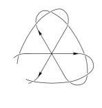
Figure 5. The separatrix diagrams represent from left to right a square-tiled surface glued from: ${\mathcal{D}}_{1}$ — one cylinder; ${\mathcal{D}}_{2}$ — two cylinders; ${\mathcal{D}}_{3}$ — not realizable by a square-tiled surface.

We reproduce now the original computation of M. Kontsevich of the volume of the stratum ${\mathcal{H}}(2)$; see [Zor2] for details.

Example of calculation of the Masur–Veech volume. Any square-tiled surface in ${\mathcal{H}}(2)$ corresponds to one of the two separatrix diagrams ${\mathcal{D}}_{1},{\mathcal{D}}_{2}$ in Figure 5. Consider those square-tiled surfaces from $\mathcal{H}(2)$ which correspond to the leftmost diagram, that is to ${\mathcal{D}}_{1}$. In this case our surface is glued from a single cylinder. The waist curve of the cylinder has length $w=\ell_{1}+\ell_{2}+\ell_{3}$, where $\ell_{1},\ell_{2},\ell_{3}$ are the integer lengths of the horizontal saddle connections (also called separatrix loops). Denote the height of the cylinder by $h_{1}$. Note that there is one more integer parameter determining our square-tiled surface: the integer twist $\phi$ which we apply to glue together the two boundary components of the cylinder. It has an integer value in the interval $[1,w]$. Thus the number of square-tiled surfaces of this type with area bounded by $N$ is asymptotically equivalent to the sum

$$\cfrac{1}{3}\sum_{\begin{subarray}{c}\ell_{1},\ell_{2},\ell_{3},h\in\mathbb{N}\\ (\ell_{1}+\ell_{2}+\ell_{3})h\leq N\end{subarray}}(\ell_{1}+\ell_{2}+\ell_{3})\,.$$

The coefficient $1/3$ compensates the arbitrariness of the choice of numbering of $\ell_{1},\ell_{2},\ell_{3}$ preserving the cyclic ordering. In other words, the order $|\Gamma({\mathcal{D}}_{1})|$ of the symmetry group of the separatrix diagram ${\mathcal{D}}_{1}$ is equal to three (the vertices of any separatrix diagram are numbered, while the edges are not). We can group the entries in the sum above having the same length $w$ of the waist curve of the cylinder. The number of ordered partitions of a large integer $w$ into the sum of three positive integers $w=\ell_{1}+\ell_{2}+\ell_{3}$ equals approximately $w^{2}/2$. Thus we can rewrite the sum above as follows:

(A.8) $$\frac{1}{3}\sum_{\begin{subarray}{c}\ell_{1},\ell_{2},\ell_{3},h\\ (\ell_{1}+\ell_{2}+\ell_{3})h\leq N\end{subarray}}(\ell_{1}+\ell_{2}+\ell_{3})\sim\frac{1}{3}\sum_{\begin{subarray}{c}w,h\\ w\cdot h\leq N\end{subarray}}w\cdot\frac{w^{2}}{2}=\frac{1}{6}\ \sum_{\begin{subarray}{c}w,h\\ w\leq\frac{N}{h}\end{subarray}}w^{3}\sim\\ \sim\frac{1}{6}\ \sum_{h\in\mathbb{N}}\frac{1}{4}\cdot\left(\frac{N}{h}\right)^{4}=\frac{N^{4}}{24}\cdot\sum_{h\in\mathbb{N}}\frac{1}{h^{4}}=\frac{N^{4}}{24}\cdot\zeta(4)=\frac{N^{4}}{24}\cdot\frac{\pi^{4}}{90}\,.$$

Consider now a square-tiled surface corresponding to the middle diagram ${\mathcal{D}}_{2}$ on Figure 5. The only admissible way to paste horizontal cylinders into this diagram is drawn on Figure 6 indicating how the boundary components are coupled.

Figure 6. The colors on the ribbon graph associated to the separatrix diagram indicate how to paste in the horizontal cylinders.

Denote the integer lengths of the separatrix loops by $\ell_{1},\ell_{2},\ell_{3}$ (see Figure 5). The realizability condition imposes the linear relation $\ell_{1}=\ell_{3}$. The flat surface $S$ is glued from two cylinders: one having the waist curve of length $\ell_{1}$, and the other one having the waist curve of length $\ell_{1}+\ell_{2}$. Denote the heights and twists of the corresponding cylinders by $h_{1},h_{2}$ and by $\phi_{1},\phi_{2}$ respectively. The integer twist of the first cylinder takes value in the interval $[1,\ell_{1}]$; the integer twist of the second cylinder takes value in the interval $[1,\ell_{1}+\ell_{2}]$. Thus, the number of surfaces of 2-cylinder type with area bounded by $N$ is asymptotically equivalent to the value of the sum

(A.9) $$\sum_{\begin{subarray}{c}\ell_{1},\ell_{2},h_{1},h_{2}\\ \ell_{1}h_{1}+(\ell_{1}+\ell_{2})h_{2}\leq N\end{subarray}}\ell_{1}(\ell_{1}+\ell_{2})=\sum_{\begin{subarray}{c}\ell_{1},\ell_{2},h_{1},h_{2}\\ \ell_{1}(h_{1}+h_{2})+\ell_{2}h_{2}\leq N\end{subarray}}\ell_{1}^{2}+\ell_{1}\ell_{2}\,.=\\ =\cfrac{N^{4}}{24}\big{[}2\cdot\zeta(1,3)+\zeta(2,2)\big{]}=\cfrac{N^{4}}{24}\left[2\cdot\cfrac{\zeta(4)}{4}+\cfrac{3\zeta(4)}{4}\right]=\cfrac{N^{4}}{24}\cdot\cfrac{5}{4}\cdot\cfrac{\pi^{4}}{90}$$

(see §5 in [Zor2] for details of the calculation).

Adding the contributions of the two diagrams and applying $\left.2\frac{d}{dN}\right|_{N=1}$ we finally get

$$\operatorname{Vol}\mathcal{H}_{1}(2)=\cfrac{\pi^{4}}{120}\,.$$

Appendix B Impact of the choice of the integer lattice on diagram-by-diagram counting of Masur–Veech volumes

Recall the following two natural choices of the integer lattice in period coordinates of a stratum of quadratic differentials.

1. the subset of $H^{1}_{-}(\hat{S},\{\hat{P}_{1},\dots,\hat{P}_{r}\};\mathbb{C})$ consisting of those linear forms which take values in $\mathbb{Z}\oplus i\mathbb{Z}$ on $H_{1}^{-}(\hat{S},\{\hat{P}_{1},\dots,\hat{P}_{r}\};\mathbb{Z})$

2. $H^{1}_{-}(\hat{S},\{\hat{P}_{1},\dots,\hat{P}_{r}\};\mathbb{C})\cap H^{1}(\hat{S},\{\hat{P}_{1},\dots,\hat{P}_{r}\};\mathbb{Z}\oplus i\mathbb{Z})$

Here we do not mark the preimages of simple poles, i.e. $\hat{P}_{1},\dots,\hat{P}_{r}$ are preimages of zeroes of the quadratic differential under the double cover. The difference between the two choices affects the linear holonomy along saddle connections joining two distinct zeroes. Under the first convention the linear holonomy along such saddle connections belongs to the half integer lattice $\frac{1}{2}\mathbb{Z}\oplus\frac{i}{2}\mathbb{Z}$ while under the second convention it belongs to the integer lattice $\mathbb{Z}\oplus i\mathbb{Z}$. This implies that the first lattice in the period coordinates is a proper sublattice of index $4^{s-1}$ of the second one, where $s$ is the number of zeroes of the quadratic differential.

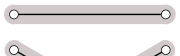
Figure 7. A separatrix diagram for ${\mathcal{Q}}(1^{2},-1^{6})$

Thus, in the case of the stratum ${\mathcal{Q}}(1^{2},-1^{6})$, it is a sublattice of index $4$. Note, however, that the contributions of individual separatrix diagrams change by the factors, which are, in general, different from the index of one lattice in the other. Consider, for example the separatrix diagram as in Figure 7 representing the stratum ${\mathcal{Q}}(1^{2},-1^{6})$. The absolute contribution of this separatrix diagram is twice bigger under the first choice of the lattice than under the second one. Indeed, under the first choice of the lattice in period coordinates, the parameter $\ell_{1}$ is half-integer, as well as all the other parameters $\ell_{2},\dots,\ell_{6},h,\phi$, (where $h,\phi$ are the height and the twist of the single cylinder) whereas $\ell_{1}$ is integer under the second choice of the lattice, and the other parameters are half-integers. Hence, the number of partitions of a given natural number $w$ (representing the length of the waist curve of the single cylinder) into the sum

$$w=2(\ell_{1}+\ell_{2}+\ell_{3}+\ell_{4}+\ell_{5})$$

is asymptotically twice bigger under the first choice of the lattice.

Now let us perform the computation for this diagram under the first convention of the choice of the lattice. When the zeroes and poles are not labeled, the diagram has symmetry of order $4$. Since the twist $\phi$ is half-integer, there are $2w$ choices of $\phi$. Recall also, that the standard pillow as in Figure 4 has area $1/2$. Thus, under the first choice of the lattice in period coordinates, the number of pillowcase covers of order at most $N$ corresponding to this separatrix diagram has the following asymptotics as $N\to+\infty$ (compare to computation (A.8)):

$$\frac{1}{4}\sum_{\begin{subarray}{c}\ell_{1},\ell_{2},\ell_{3},\ell_{4},\ell_{5},h\in\mathbb{N}/2\\ (2(\ell_{1}+\ell_{2}+\ell_{3}+\ell_{4}+\ell_{5}))\cdot h\leq N/2\end{subarray}}2(2(\ell_{1}+\ell_{2}+\ell_{3}+\ell_{4}+\ell_{5}))\sim\frac{1}{4}\sum_{\begin{subarray}{c}w,H\in\mathbb{N}\\ w\cdot H\leq N\end{subarray}}2w\cdot\frac{w^{4}}{4!}=\\ =\frac{1}{2\cdot 4!}\ \sum_{\begin{subarray}{c}w,H\in\mathbb{N}\\ w\leq\frac{N}{H}\end{subarray}}w^{5}\sim\frac{1}{2\cdot 4!}\ \sum_{H\in\mathbb{N}}\frac{1}{6}\cdot\left(\frac{N}{H}\right)^{6}=\frac{N^{6}}{12\cdot 4!}\cdot\sum_{H\in\mathbb{N}}\frac{1}{H^{6}}=\frac{N^{6}}{12\cdot 4!}\cdot\zeta(6)\,.$$

Here in the first equivalence we passed from the half-integer parameter $h$ to the integer parameter $H=2h$ replacing the condition $wh\leq N/2$ by the equivalent condition $wH\leq N$. Applying $\left.2\frac{d}{dN}\right|_{N=1}$ and multiplying by the factor $6!\cdot 2!$ responsible for numbering of zeroes and poles, we get the total contribution $60\zeta(6)$ to the volume $\operatorname{Vol}^{(1)}{\mathcal{Q}}^{numbered}_{1}(1^{2},-1^{6})$ defined under the first convention on the choice of the lattice.

Similar computations for each separatrix diagram in this stratum are cumbersome, so, following [AEZor1], we distribute the diagrams into groups organized in the following way.

Each connected component of the separatrix diagram is encoded by a vertex of a graph decorated with an ordered pair of natural numbers indicating the number of zeroes and poles living at the corresponding component. A flat cylinder joining two connected components of a separatrix diagram is encoded by an edge of the graph. For example, the separatrix diagram from Figure 7 contains two connected components joined by a single cylinder. The corresponding graph contains two vertices joined by a single edge; one vertex is decorated with the pair $(2,4)$ (standing for $2$ zeroes and $4$ poles) and the other vertex is decorated with the pair $(0,2)$ (standing for $0$ zeroes and $2$ poles). This graph is the top entry of the left column in Table 2.

$$\begin{array}[]{|c|c|c|}\hline\cr\text{Tree}&\text{Contribution to }\operatorname{Vol}^{(1)}&\cfrac{\text{Contribution to }\operatorname{Vol}^{(1)}}{\text{Contribution to }\operatorname{Vol}^{(2)}}\\[-6.0pt] &&\\ \hline\cr&&\\ \begin{picture}(35.0,10.0)(0.0,0.0)\put(0.0,0.0){\circle{4.0}} \put(-5.0,5.0){\tiny 2,4} \put(2.0,0.0){\line(1,0){26.0}} \put(30.0,0.0){\circle{4.0}} \put(25.0,5.0){\tiny 0,2} \end{picture}&60\zeta(6)&2\\ &&\\ \hline\cr&&\\ \begin{picture}(35.0,10.0)(0.0,0.0)\put(0.0,0.0){\circle{4.0}} \put(-5.0,5.0){\tiny 1,3} \put(2.0,0.0){\line(1,0){26.0}} \put(30.0,0.0){\circle{4.0}} \put(25.0,5.0){\tiny 1,3} \end{picture}&80\zeta(6)&2^{7}\\ &&\\ \hline\cr&&\\ \begin{picture}(70.0,10.0)(-5.0,0.0)\put(0.0,0.0){\circle{4.0}} \put(-5.0,5.0){\tiny 0,2} \put(2.0,0.0){\line(1,0){26.0}} \put(30.0,0.0){\circle{4.0}} \put(25.0,5.0){\tiny 2,2} \put(32.0,0.0){\line(1,0){26.0}} \put(60.0,0.0){\circle{4.0}} \put(55.0,5.0){\tiny 0,2} \end{picture}&72\zeta(2)\zeta(4)&2\\ &&\\ \hline\cr&&\\ \begin{picture}(70.0,10.0)(-5.0,0.0)\put(0.0,0.0){\circle{4.0}} \put(-5.0,5.0){\tiny 1,3} \put(2.0,0.0){\line(1,0){26.0}} \put(30.0,0.0){\circle{4.0}} \put(25.0,5.0){\tiny 1,1} \put(32.0,0.0){\line(1,0){26.0}} \put(60.0,0.0){\circle{4.0}} \put(55.0,5.0){\tiny 0,2} \end{picture}&48\zeta(2)\zeta(4)&2^{5}\\ &&\\ \hline\cr&&\\ \begin{picture}(100.0,10.0)(-5.0,0.0)\put(0.0,0.0){\circle{4.0}} \put(-5.0,5.0){\tiny 0,2} \put(2.0,0.0){\line(1,0){26.0}} \put(30.0,0.0){\circle{4.0}} \put(25.0,5.0){\tiny 1,1} \put(32.0,0.0){\line(1,0){26.0}} \put(60.0,0.0){\circle{4.0}} \put(55.0,5.0){\tiny 1,1} \put(62.0,0.0){\line(1,0){26.0}} \put(90.0,0.0){\circle{4.0}} \put(85.0,5.0){\tiny 0,2} \end{picture}&24\zeta^{3}(2)&2^{3}\\ &&\\ \hline\cr&&\\ \begin{picture}(70.0,10.0)(-5.0,5.0)\put(0.0,0.0){\circle{4.0}} \put(-5.0,5.0){\tiny 0,2} \put(2.0,0.0){\line(1,0){26.0}} \put(30.0,0.0){\circle{4.0}} \put(25.0,5.0){\tiny 2,0} \put(32.0,0.0){\line(2,1){26.0}} \put(60.0,14.0){\circle{4.0}} \put(65.0,14.0){\tiny 0,2} \put(32.0,0.0){\line(2,-1){26.0}} \put(60.0,-14.0){\circle{4.0}} \put(65.0,-14.0){\tiny 0,2} \end{picture}&4\zeta^{3}(2)&2\\ &&\\ &&\\ \hline\cr\end{array}$$

Table 2. Table of diagram contributions to the Masur–Veech volume $\operatorname{Vol}{\mathcal{Q}}_{1}(1^{2},-1^{6})$ in normalizations $(1)$ and $(2)$

Note that the stratum ${\mathcal{Q}}(1^{2},-1^{6})$ corresponds to genus zero, so the underlying topological surface is a sphere. This implies that the graph defined by a separatrix diagram representing the stratum ${\mathcal{Q}}(1^{2},-1^{6})$ is, actually, a tree. The first column of Table 2 provides the list of all possible decorated trees which appear for the stratum ${\mathcal{Q}}(1^{2},-1^{6})$. It is easy to verify that the ratio of contributions of a given separatrix diagram to the volume of the stratum ${\mathcal{Q}}(1^{r},-1^{r+4})$ computed under the two conventions on the choice of the integer lattice depends only on the corresponding decorated tree. We group together all the diagrams corresponding to each decorated tree and indicated in the second column the corresponding contribution to the volume under the first choice of the lattice (using [AEZor1, §3.8] as the source). In the third column we give the ratio of the contributions represented by the corresponding tree. For example, the tree in the first line represents the unique diagram shown in Figure 7; as it was computed above its contribution to the volume under the first choice of the lattice is $60\zeta(6)$ and the contribution to the volume under the second choice of the lattice is twice smaller. These data constitute the first line of Table 2.

Recall that the normalization factor between the two lattices in the period coordinates of the stratum ${\mathcal{Q}}(1^{2},-1^{6})$ is $4$. However, observing Table 2 the reader can see that the individual contributions of diagrams differ by factors $2$, $2^{3}$, $2^{5}$, $2^{7}$.

Note that the trees with the same number of edges provide contributions of the same “arithmetic” nature, namely the total contribution of $1,2,3$-cylinder diagrams are

$$140\zeta(6)+120\zeta(2)\zeta(4)+28\zeta^{3}(2)=\cfrac{\pi^{6}}{2}=\operatorname{Vol}^{(1)}{\mathcal{Q}}(1^{2},-1^{6})$$

respectively under the first choice of the lattice and

$$\frac{245}{8}\zeta(6)+\frac{75}{2}\zeta(2)\zeta(4)+5\zeta^{3}(2)=\cfrac{\pi^{6}}{8}=\operatorname{Vol}^{(2)}{\mathcal{Q}}(1^{2},-1^{6})$$

respectively under the second choice. The volumes $\operatorname{Vol}^{(1)}$ and $\operatorname{Vol}^{(2)}$ differ by the factor $4$ as expected.

We get a polynomial identity

$$140\zeta(6)+120\zeta(2)\zeta(4)+28\zeta^{3}(2)=\cfrac{\pi^{6}}{2}=4\Big{(}\frac{245}{8}\zeta(6)+\frac{75}{2}\zeta(2)\zeta(4)+5\zeta^{3}(2)\Big{)}$$

in zeta values at even integers. Considering other strata ${\mathcal{Q}}(1^{r},-1^{r+4})$ we get an infinite series of analogous identities in zeta values at even integers.

We did not study the identities resulting from different choices of the lattice in period coordinates for more general strata of meromorphic quadratic differentials with at most simple poles in genus zero. Considering zeroes of even order might produce identities of much more elaborate arithmetic nature.

If our guess that the contribution of $k$-cylinder square-tiled surfaces to a given stratum of Abelian differentials is a polynomial in multiple zeta values with rational (or even integer) coefficients is true, then playing with different choices of an integer lattice we will get infinite series of mysterious polynomial identities in multiple zeta values.

Another challenge is to see whether one can obtain some information about volume asymptotics for large genera playing with the choice of an integer lattice. We leave both questions as a problem, which might be interesting to study.

Problem.

Describe and study polynomial identities on multiple zeta values arising from $k$-cylinder contributions to the Masur–Veech volumes under different choices of integer lattices in period coordinates. Study these identities in asymptotic regimes when the genus of the surface or the number of simple poles tends to infinity.

Appendix C Tables of the Masur–Veech volumes of low-dimensional strata in the moduli spaces of meromorphic quadratic differentials with at most simple poles

In the tables below we present the volumes of all low-dimensional strata of quadratic differentials up to dimension $d=6$. The approximate values of Masur–Veech volumes were actively used in the papers [Gj1] and [Gj2] to debug the rigorous theoretically found values of the Masur–Veech volumes of the strata of quadratic differentials and related Siegel–Veech constants.

Each table is organized as follows.

The left column indicates the stratum ${\mathcal{Q}}(d_{1},\dots,d_{k})$. The second column provides the rigorous rational number $r$ in the absolute contribution, see (2.2),

$$c_{1}(d_{1},\dots,d_{k})=r\cdot\zeta(d)$$

of $1$-cylinder pillowcase covers to the Masur–Veech volume $\operatorname{Vol}{\mathcal{Q}}(d_{1},\dots,d_{k})$.

The third column provides experimental statistical data, namely, the approximate proportions of the number of square-tiled surfaces with $1$ cylinder, $2$-cylinders, and so on tiled with tiny squares.

Combining data from the second and the third column, we provide in the fourth column the resulting approximate value of the volume obtained experimentally.

In the right two columns we present the value of the Masur–Veech volume of the corresponding stratum obtain by rigorous methods, namely, the approximate numerical value in the second column from the right and the exact value in the rightmost column.

The rightmost column contains a symbol indicating the rigorous methods of computation of the exact value of the Masur–Veech volumes of the stratum under consideration (see [Gj2] for more details):

• By the results of Eskin–Okounkov [EO2], the generating functions for the number of pillowcase covers are quasimodular. The volumes are derived from the asymptotics of these functions, which can be easily computed using the quasimodularity property. Note that this method do not give the volumes of the connected components of the strata.

• For the case of genus $0$ surfaces, there exists a closed formula for volumes, that was conjectured by Kontsevich and then proved by Athreya–Eskin–Zorich in [AEZor1] and [AEZor2].

• For hyperelliptic components, volumes are easily deduced from the volumes of strata of genus $0$ surfaces.

• Some strata have a special property: they are non-varying, meaning that the Lyapunov spectrum (and so the Siegel–Veech constant) is the same for any Teichmüller curve, see [CMö]. The volume is then deduced from the (common value of the) Siegel–Veech constant using the technics of Masur–Zorich (see [Gj1]);

• Finally, as for $1$-cylinder surfaces, the volumes of low-dimensional strata can be computed diagram by diagram.

We always use normalization as in [AEZor2]; see also Convention A.1.

Strata of dimension $4$

$$\begin{array}[]{|c|c|c|c|c|c|}\hline\cr&&&&\vrule\lx@intercol\hfil\hfil\lx@intercol\vrule\lx@intercol\\[-6.0pt] \text{Component}&\text{Abs. contr.}&\text{Statistics of}&\text{Experim.}&\vrule\lx@intercol\hfil\text{Theoretical value}\hfil\lx@intercol\vrule\lx@intercol\\ \text{of the}&r\cdot\zeta(4)\text{ of}&\text{frequency of}&\text{value}&\vrule\lx@intercol\hfil\text{of the volume}\hfil\lx@intercol\vrule\lx@intercol\\ \cline{5-6}\cr\text{stratum}&\text{1-cylinder}&1:2:\cdots-\text{cylinder}&\text{of the}&&\\ &\text{surfaces}&\text{surfaces}&\text{volume}&\text{Approx.}&\text{Exact}\\[-6.0pt] &&&&&\\ \hline\cr\lx@intercol\hfil\hfil\lx@intercol\\[-6.0pt] \lx@intercol\hfil\hfil\lx@intercol\\[-6.0pt] \lx@intercol\hfil\text{genus 0}\hfil\lx@intercol\\ \lx@intercol\hfil\hfil\lx@intercol\\[-6.0pt] \hline\cr&&&&&\\[-6.0pt] {\mathcal{Q}}(1,-1^{5})&40&0.4382:0.5618&1.014\cdot\pi^{4}&1.000\cdot\pi^{4}&{\pi^{4}}\\ &&0.4444:0.5556&&&\\ &&\frac{4}{9}:\frac{5}{9}&&&\textrm{g0},\textrm{EO}\\[-6.0pt] &&&&&\\ \hline\cr\lx@intercol\hfil\hfil\lx@intercol\\[-6.0pt] \lx@intercol\hfil\hfil\lx@intercol\\[-6.0pt] \lx@intercol\hfil\text{genus 1}\hfil\lx@intercol\\ \lx@intercol\hfil\hfil\lx@intercol\\[-6.0pt] \hline\cr&&&&&\\[-6.0pt] {\mathcal{Q}}(1^{2},-1^{2})&50/3&0.5724:0.4276&0.324\cdot\pi^{4}&0.3333\cdot\pi^{4}&{\frac{1}{3}\cdot\pi^{4}}\\ &&0.5556:0.4444&&&\\ &&\frac{4}{9}:\frac{5}{9}&&&\textrm{hyp},\textrm{diag},\textrm{EO}\\[-6.0pt] &&&&&\\ \hline\cr&&&&&\\[-6.0pt] {\mathcal{Q}}(3,-1^{3})&30&0.6016:0.3984&0.554\cdot\pi^{4}&0.5556\cdot\pi^{4}&{\frac{5}{9}\cdot\pi^{4}}\\ &&0.6000:0.4000&&&\\ &&\frac{3}{5}:\frac{2}{5}&&&\textrm{diag},\textrm{nv},\textrm{EO}\\[-6.0pt] &&&&&\\ \hline\cr\lx@intercol\hfil\hfil\lx@intercol\\[-6.0pt] \lx@intercol\hfil\hfil\lx@intercol\\[-6.0pt] \lx@intercol\hfil\text{genus 2}\hfil\lx@intercol\\ \lx@intercol\hfil\hfil\lx@intercol\\[-6.0pt] \hline\cr&&&&&\\[-6.0pt] {\mathcal{Q}}(2^{2})&17/4&0.7065:0.2130:0.0805&{0.666}\cdot\pi^{2}&0.6666\cdot\pi^{2}&{\frac{2}{3}\cdot\pi^{2}}\\ &&0.6991:0.2089:0.0920&&&\\ &&&&&\textrm{hyp},\textrm{diag},\textrm{EO}\\[-6.0pt] &&&&&\\ \hline\cr&&&&&\\[-6.0pt] {\mathcal{Q}}(5,-1)&12&0.6488:0.3512&0.206\cdot\pi^{4}&0.2074\cdot\pi^{4}&{\frac{28}{135}\cdot\pi^{4}}\\ &&0.6429:0.3571&&&\\ &&\frac{9}{14}:\frac{5}{14}&&&\textrm{diag},\textrm{nv},\textrm{EO}\\[-6.0pt] &&&&&\\ \hline\cr\end{array}$$

For ${\mathcal{Q}}(2^{2})$ the exact proportions are more bulky, so we give them separately:

$$\text{Frequences for }{\mathcal{Q}}(2,2):\quad\frac{17\zeta(4)}{4}\ :\ 16\zeta(3)-\frac{33}{2}\zeta(4)\ :\ 4\zeta(2)-16\zeta(3)+\frac{49\zeta(4)}{4}\,.$$

Strata of dimension $5$

$$\begin{array}[]{|c|c|c|c|c|c|}\hline\cr&&&&\vrule\lx@intercol\hfil\hfil\lx@intercol\vrule\lx@intercol\\[-6.0pt] \text{Component}&\text{Abs. contr.}&\text{Statistics of}&\text{Experim.}&\vrule\lx@intercol\hfil\text{Theoretical value}\hfil\lx@intercol\vrule\lx@intercol\\ \text{of the}&r\cdot\zeta(5)\text{ of}&\text{frequency of}&\text{value}&\vrule\lx@intercol\hfil\text{of the volume}\hfil\lx@intercol\vrule\lx@intercol\\ \cline{5-6}\cr\text{stratum}&\text{1-cylinder}&1:2:\cdots-\text{cylinder}&\text{of the}&&\\ &\text{surfaces}&\text{surfaces}&\text{volume}&\text{Approx.}&\text{Exact}\\[-6.0pt] &&&&&\\ \hline\cr\lx@intercol\hfil\hfil\lx@intercol\\[-6.0pt] \lx@intercol\hfil\hfil\lx@intercol\\[-6.0pt] \lx@intercol\hfil\text{genus 0}\hfil\lx@intercol\\ \lx@intercol\hfil\hfil\lx@intercol\\[-6.0pt] \hline\cr&&&&&\\[-6.0pt] {\mathcal{Q}}(2,-1^{6})&60&0.2472:0.6740:0.0789&2.584\cdot\pi^{4}&2.666\cdot\pi^{4}&{\frac{8}{3}\cdot\pi^{4}}\\ &&0.2395:\phantom{0.4854}:\phantom{0.4854}&&&\textrm{g0},\textrm{EO}\\[-6.0pt] &&&&&\\ \hline\cr\lx@intercol\hfil\hfil\lx@intercol\\[-6.0pt] \lx@intercol\hfil\hfil\lx@intercol\\[-6.0pt] \lx@intercol\hfil\text{genus 1}\hfil\lx@intercol\\ \lx@intercol\hfil\hfil\lx@intercol\\[-6.0pt] \hline\cr&&&&&\\[-6.0pt] {\mathcal{Q}}(2,1,-1^{3})&45&0.4919:0.4472:0.0610&0.974\cdot\pi^{2}&\pi^{4}&{\pi^{4}}\\ &&0.4790:\phantom{0.4854}:\phantom{0.4854}&&&\textrm{nv},\textrm{EO}\\[-6.0pt] &&&&&\\ \hline\cr&&&&&\\[-6.0pt] {\mathcal{Q}}(4,-1^{4})&84&0.4309:0.5163:0.0528&2.075\cdot\pi^{2}&2\cdot\pi^{4}&{2\cdot\pi^{4}}\\ &&0.4471:\phantom{0.4854}:\phantom{0.4854}&&&\textrm{nv},\textrm{EO}\\[-6.0pt] &&&&&\\ \hline\cr\lx@intercol\hfil\hfil\lx@intercol\\[-6.0pt] \lx@intercol\hfil\hfil\lx@intercol\\[-6.0pt] \lx@intercol\hfil\text{genus 2}\hfil\lx@intercol\\ \lx@intercol\hfil\hfil\lx@intercol\\[-6.0pt] \hline\cr&&&&&\\[-6.0pt] {\mathcal{Q}}(2,1^{2})&11/2&0.4398:0.4667:0.0935&0.133\cdot\pi^{4}&0.1333\cdot\pi^{4}&{\frac{2}{15}\cdot\pi^{4}}\\ &&0.4391:0.4621:0.0988&&&\textrm{hyp},\textrm{diag},\textrm{EO}\\[-6.0pt] &&&&&\\ \hline\cr&&&&&\\[-6.0pt] {\mathcal{Q}}(4,1,-1)&68/3&0.4772:0.4854:0.0374&0.506\cdot\pi^{4}&0.5333\cdot\pi^{4}&{\frac{8}{15}\cdot\pi^{4}}\\ &&0.4524:\phantom{0.4854}:\phantom{0.4854}&&&\textrm{nv},\textrm{EO}\\[-6.0pt] &&&&&\\ \hline\cr&&&&&\\[-6.0pt] {\mathcal{Q}}(3,2,-1)&115/6&0.5528:0.3813:0.0659&0.369\cdot\pi^{4}&0.3704\cdot\pi^{4}&{\frac{10}{27}\cdot\pi^{4}}\\ &&0.5509:\phantom{0.4854}:\phantom{0.4854}&&&\textrm{nv},\textrm{EO}\\[-6.0pt] &&&&&\\ \hline\cr&&&&&\\[-6.0pt] {\mathcal{Q}}^{hyp}(6,-1^{2})&65/12&0.3057:0.6374:0.0569&0.189\cdot\pi^{4}&0.1777\cdot\pi^{4}&{\frac{8}{45}\cdot\pi^{4}}\\ &&0.3243:\phantom{0.4854}:\phantom{0.4854}&&&\textrm{hyp}\\[-6.0pt] &&&&&\\ \cline{1-6}\cr&&&&&\\[-6.0pt] {\mathcal{Q}}^{non}(6,-1^{2})&181/3&0.5366:0.4008:0.0626&1.197\cdot\pi^{4}&1.1852\cdot\pi^{4}&{\frac{32}{27}\cdot\pi^{4}}\\ &&0.5419:\phantom{0.4854}:\phantom{0.4854}&&&\textrm{nv},\textrm{EO}\\[-6.0pt] &&&&&\\ \hline\cr\lx@intercol\hfil\hfil\lx@intercol\\[-6.0pt] \lx@intercol\hfil\hfil\lx@intercol\\[-6.0pt] \lx@intercol\hfil\text{genus 3}\hfil\lx@intercol\\ \lx@intercol\hfil\hfil\lx@intercol\\[-6.0pt] \hline\cr&&&&&\\[-6.0pt] {\mathcal{Q}}(8)&56/3&0.5211:0.4024:0.0764&0.381\cdot\pi^{4}&0.3704\cdot\pi^{4}&\frac{10}{27}\cdot\pi^{4}\\ &&&&&\textrm{EO}\\[-6.0pt] &&&&&\\ \hline\cr\end{array}$$

Exact values of frequences of $1:2:3$-cylinder square-tiled surfaces for ${\mathcal{Q}}(2,1^{2})$ are:

$$\frac{11\zeta(5)}{2}\ :\ 3\zeta(2)\zeta(3)+\frac{16\zeta(4)}{3}-\frac{11\zeta(5)}{2}\ :\ \zeta(2)(\frac{8\zeta(2)}{3}-3\zeta(3))$$

Strata of dimension $6$

$$\begin{array}[]{|c|c|c|c|c|c|}\hline\cr&&&&\vrule\lx@intercol\hfil\hfil\lx@intercol\vrule\lx@intercol\\[-6.0pt] \text{Component}&\text{Abs.\! cont.}&\text{Statistics of}&\text{Experim.}&\vrule\lx@intercol\hfil\text{Theoretical value}\hfil\lx@intercol\vrule\lx@intercol\\ \text{of the}&r\cdot\zeta(6)\text{ of}&\text{frequency of}&\text{value}&\vrule\lx@intercol\hfil\text{of the volume}\hfil\lx@intercol\vrule\lx@intercol\\ \cline{5-6}\cr\text{stratum}&\text{1-cylinder}&1:2:\cdots-\text{cylinder}&\text{of the}&&\\ &\text{surfaces}&\text{surfaces}&\text{volume}&\text{Approx.}&\text{Exact}\\[-6.0pt] &&&&&\\ \hline\cr\lx@intercol\hfil\hfil\lx@intercol\\[-6.0pt] \lx@intercol\hfil\hfil\lx@intercol\\[-6.0pt] \lx@intercol\hfil\text{genus 0}\hfil\lx@intercol\\ \lx@intercol\hfil\hfil\lx@intercol\\[-6.0pt] \hline\cr&&&&&\\[-6.0pt] {\mathcal{Q}}(1^{2},-1^{6})&140&\text{0.2943:0.4236:0.2821}&0.5034\cdot\pi^{6}&0.5000\cdot\pi^{6}&{\frac{1}{2}\cdot\pi^{6}}\\[-6.0pt] &&&&&\\ \hline\cr&&&&&\\[-6.0pt] {\mathcal{Q}}(3,-1^{7})&84&\text{0.1106:0.6187:0.2707}&0.8037\cdot\pi^{6}&0.8000\cdot\pi^{6}&{\frac{3}{4}\cdot\pi^{6}}\\[-6.0pt] &&&&&\\ \hline\cr\lx@intercol\hfil\hfil\lx@intercol\\[-6.0pt] \lx@intercol\hfil\hfil\lx@intercol\\[-6.0pt] \lx@intercol\hfil\text{genus 1}\hfil\lx@intercol\\ \lx@intercol\hfil\hfil\lx@intercol\\[-6.0pt] \hline\cr&&&&&\\[-6.0pt] {\mathcal{Q}}(1^{3},-1^{3})&77&\text{0.4366:0.4000:0.1634}&0.1866\cdot\pi^{6}&{0.1837\cdot\pi^{6}}&\frac{11}{60}\cdot{\pi^{6}}\\[-6.0pt] &&&&&\\ \hline\cr&&&&&\\[-6.0pt] {\mathcal{Q}}(3,1,-1^{4})&126&\text{0.4000:0.4520:0.1480}&0.3333\cdot\pi^{6}&0.3333\cdot\pi^{6}&{\frac{1}{3}\cdot\pi^{6}}\;(\textrm{nv})\\[-6.0pt] &&&&&\\ \hline\cr&&&&&\\[-6.0pt] {\mathcal{Q}}(2^{2},-1^{4})&110&\text{0.364:0.511:0.108:0.016}&3.1544\cdot\pi^{4}&{3.0222\cdot\pi^{4}}&\frac{136}{45}\cdot\pi^{4}\\[-6.0pt] &&&&&\\ \hline\cr&&&&&\\[-6.0pt] {\mathcal{Q}}(5,-1^{5})&210&\text{0.3276:0.5301:0.1423}&0.6783\cdot\pi^{6}&0.7000\cdot\pi^{6}&{\frac{7}{10}\cdot\pi^{6}}\;(\textrm{nv})\\[-6.0pt] &&&&&\\ \hline\cr\lx@intercol\hfil\hfil\lx@intercol\\[-6.0pt] \lx@intercol\hfil\hfil\lx@intercol\\[-6.0pt] \lx@intercol\hfil\text{genus 2}\hfil\lx@intercol\\ \lx@intercol\hfil\hfil\lx@intercol\\[-6.0pt] \hline\cr&&&&&\\[-6.0pt] {\mathcal{Q}}(1^{4})&49/3&\text{0.2512:0.5577:0.1911}&0.0688\cdot\pi^{6}&0.0666\cdot\pi^{6}&{\frac{\pi^{6}}{15}}\\[-6.0pt] &&&&&\\ \hline\cr&&&&&\\[-6.0pt] {\mathcal{Q}}(3,1^{2},-1)&119/3&\text{0.3593:0.5081:0.1325}&0.1168\cdot\pi^{6}&0.1104\cdot\pi^{6}&{\frac{1}{9}\cdot\pi^{6}}\;(\textrm{nv})\\[-6.0pt] &&&&&\\ \hline\cr&&&&&\\[-6.0pt] {\mathcal{Q}}(2^{2},1,-1)&94/3&\text{0.391:0.503:0.096:0.0098}&0.837\cdot\pi^{4}&0.8000\cdot\pi^{4}&{\frac{4}{5}\cdot\pi^{4}}\;(\textrm{nv})\\[-6.0pt] &&&&&\\ \hline\cr&&&&&\\[-6.0pt] {\mathcal{Q}}(5,1,-1^{2})&189/2&\text{0.4252:0.4569:0.1179}&0.2352\cdot\pi^{6}&0.2333\cdot\pi^{6}&{\frac{7}{30}\cdot\pi^{6}}\;(\textrm{nv})\\[-6.0pt] &&&&&\\ \hline\cr&&&&&\\[-6.0pt] {\mathcal{Q}}(4,2,-1^{2})&317/4&\text{0.450:0.449:0.089:0.012}&1.8409\cdot\pi^{4}&1.866\cdot\pi^{4}&\frac{28}{15}\cdot\pi^{4}\;(\textrm{nv})\\[-6.0pt] &&&&&\\ \hline\cr&&&&&\\[-6.0pt] {\mathcal{Q}}^{hyp}(3^{2},-1^{2})&161/30&\text{0.1724:0.6520:0.1756}&0.0329\cdot\pi^{6}&0.0333\cdot\pi^{6}&{\frac{1}{30}\cdot\pi^{6}}\\[-6.0pt] &&&&&\\ \cline{1-6}\cr&&&&&\\[-6.0pt] {\mathcal{Q}}^{nh}(3^{2},-1^{2})&1106/15&\text{0.4894:0.3951:0.1154}&0.1594\cdot\pi^{6}&0.1630\cdot\pi^{6}&{\frac{22}{135}\cdot\pi^{6}}\;(\textrm{nv})\\[-6.0pt] &&&&&\\ \hline\cr&&&&&\\[-6.0pt] {\mathcal{Q}}(7,-1^{3})&441/2&\text{0.4179:0.4626:0.1195}&0.5583\cdot\pi^{6}&0.54\cdot\pi^{6}&\frac{27}{50}\cdot{\pi^{6}}\\[-6.0pt] &&&&&\\ \hline\cr&&&&&\\[-6.0pt] {\mathcal{Q}}(7,1)&37&\text{0.3724:0.5171:0.1106}&0.1051\cdot\pi^{6}&0.1028\cdot\pi^{6}&{\frac{18}{175}\cdot\pi^{6}}\;(\textrm{nv})\\[-6.0pt] &&&&&\\ \hline\cr&&&&&\\[-6.0pt] {\mathcal{Q}}^{hyp}(6,2)&65/48&\text{0.237:0.608:0.137:0.018}&0.0597\cdot\pi^{4}&0.0593\cdot\pi^{4}&{\frac{8}{135}\cdot\pi^{4}}\\[-6.0pt] &&&&&\\ \cline{1-6}\cr&&&&&\\[-6.0pt] {\mathcal{Q}}^{nh}(6,2)&389/12&\text{0.473:0.380:0.112:0.035}&0.7155\cdot\pi^{4}&0.7111\cdot\pi^{4}&\frac{96}{135}\cdot\pi^{4}\\[-6.0pt] &&&&&\\ \hline\cr&&&&&\\[-6.0pt] {\mathcal{Q}}(5,3)&77/3&\text{0.488:0.383:0.129}&0.056\cdot\pi^{6}&0.0588\cdot\pi^{6}&\frac{14}{243}\cdot{\pi^{6}}\\[-6.0pt] &&&&&\\ \hline\cr&&&&&\\[-6.0pt] {\mathcal{Q}}(4^{2})&92/3&\text{0.388:0.481:0.109:0.022}&0.8259\cdot\pi^{4}&0.8000\cdot\pi^{4}&{\frac{4}{5}\cdot\pi^{4}}\\[-6.0pt] &&&&&\\ \hline\cr&&&&&\\[-6.0pt] {\mathcal{Q}}^{reg}(9,-1)&385/3&\text{0.4569:0.4195:0.1236}&0.2972\cdot\pi^{6}&&\\[-6.0pt] &&&&0.3580\cdot\pi^{6}&\frac{15224}{42525}\cdot{\pi^{6}}\\ {\mathcal{Q}}^{irr}(9,-1)&55/3&\text{0.3024:0.5740:0.1236}&0.0642\cdot\pi^{6}&&\\[-6.0pt] &&&&&\\ \hline\cr\end{array}$$

As before, we applied the method of Eskin–Okounkov to all strata, and methods specific for genus $0$ and for hyperelliptic components when applicable. For the non-varying strata (nv) we also used evaluation through Siegel–Veech constants.

References

• [AEZor1] J. Athreya, A. Eskin, and A. Zorich, Counting generalized Jenkins–Strebel differentials, Geometriae Dedicata, 170:1 (2014), 195–217.
• [AEZor2] J. Athreya, A. Eskin, and A. Zorich, Right-angled billiards and volumes of moduli spaces of quadratic differentials on ${\mathbb{C}}\!\operatorname{P}^{1}$, Ann. Scient. Éc. Norm. Sup. 4e série, 49 (2016), 1307–1381.
• [BL] C. Boissy, E. Lanneau, Dynamics and geometry of the Rauzy–Veech induction for quadratic differentials, Ergodic Theory Dynam. Systems 29 (2009), no. 3, 767–816.
• [CMö] D. Chen, M. Möller, Quadratic differentials in low genus: exceptional and non-varying strata, Annales de l’ENS 47:2 (2014), 309–369.
• [CMöZag] D. Chen, M. Möller, D. Zagier, Quasimodularity and large genus limits of Siegel–Veech constants, arXiv:1606.04065 (2016).
• [DaN] C. Danthony and A. Nogueira. Involutions linéaires et feuilletages mesurés, C. R. Acad. Sci. Paris, Sér. I Math. 307(8) (1988), 409–412.
• [D] V. Delecroix, Cardinality of Rauzy classes, Ann. Inst. Fourier 63 (2013), no. 5, 1651–1715.
• [DHL] V. Delecroix, P. Hubert, S. Lelivre, Diffusion for the periodic wind-tree model, Annales de l’ENS 47:6 (2014), 1085–1110.
• [DZor] V. Delecroix, A. Zorich, Cries and whispers in wind-tree forests, arXiv:1502.06405 (2015), 1–27.
• [E] A. Eskin, Volumes of even and odd components of the strata of Abelian differentials, manuscript.
• [EKZor] A. Eskin, M. Kontsevich, A. Zorich, Sum of Lyapunov exponents of the Hodge bundle with respect to the Teichmüller geodesic flow, Publications de l’IHES, 120:1 (2014), 207–333.
• [EM] A. Eskin, H. Masur, Asymptotic formulas on flat surfaces, Ergodic Theory and Dynamical Systems, 21 (2) (2001), 443–478.
• [EMZor] A. Eskin, H. Masur, A. Zorich, Moduli spaces of abelian differentials: the principal boundary, counting problems, and the Siegel-Veech constants, Publ. Math. Inst. Hautes Etudes Sci. 97 (2003), 61–179.
• [EMi] A. Eskin and M. Mirzakhani, Invariant and stationary measures for the $\operatorname{SL}(2,{\mathbb{R}})$ action on moduli space, arXiv:1302.3320 (2013).
• [EMiMo] A. Eskin, M. Mirzakhani, A. Mohammadi, Isolation, equidistribution, and orbit closures for the $\operatorname{SL}(2,{\mathbb{R}})$-action on moduli space, Ann. of Math. 182 (2015), no. 2, 673–721.
• [EO1] A. Eskin, A. Okounkov. Asymptotics of numbers of branched coverings of a torus and volumes of moduli spaces of holomorphic differentials, Invent. Math. 145 (2001), no. 1, 59–103.
• [EO2] A. Eskin, A. Okounkov. Pillowcases and quasimodular forms, Algebraic Geometry and Number Theory, Progress in Mathematics 253 (2006), 1–25.
• [EOP] A. Eskin, A. Okounkov, R. Pandharipande, The theta characteristic of a branched covering, Adv. Math., 217 no. 3 (2008), 873–888.
• [EZor] A. Eskin, A. Zorich, Volumes of strata of Abelian differentials and Siegel–Veech constants in large genera, Arnold Mathematical Journal, 1:4 (2015), 481–488.
• [Fo] G. Forni, Deviation of ergodic averages for area-preserving flows on surfaces of higher genus, Annals of Math., 155 no. 1 (2002), 1–103.
• [Gj1] E. Goujard, Siegel–Veech constants and volumes of strata of moduli spaces of quadratic differentials, Geom. Funct. Anal. 25 (2015), no. 5, 1440–1492. .
• [Gj2] E. Goujard, Volumes of strata of moduli spaces of quadratic differentials: getting explicit values, Ann. Inst. Fourier, 66 no. 6 (2016), 2203–2251.
• [GjMö] E. Goujard, M. Möller, Counting Feynman-like graphs: Quasimodularity and Siegel-Veech weight , arXiv:1609.01658 (2016).
• [Gd] H. W. Gould, Combinatorial identities. A standardized set of tables listing 500 binomial coefficient summations. Rev. ed. (English) Morgantown (1972).
• [KaZog] M. Kazarian, P. Zograf, Virasoro constraints and topological recursion for Grothendieck’s dessin counting, Lett. Math. Phys. 105 (2015), no. 8, 1057–1084.
• [KZ] M. Kontsevich, A. Zorich. Connected components of the moduli spaces of Abelian differen- tials with prescribed singularities, Invent. Math., 153 (2003), no.3, 631–678.
• [L] E. Lanneau, Connected components of the strata of the moduli spaces of quadratic differentials, Annales de l’ENS 41 no. 1 (2008), 1–56.
• [Ma] H. Masur, Interval exchange transformations and measured foliations, Ann. of Math., 115 (1982), 169–200.
• [Mi1] M. Mirzakhani, Growth of the number of simple closed geodesics on hyperbolic surfaces, Annals of Math. (2) 168 (2008), no. 1, 97–125.
• [S] K. Strebel, Quadratic differentials, Springer-Verlag, 1984.
• [Ve1] W. Veech, Gauss measures for transformations on the space of interval exchange maps, Annals of Math., 115 (1982), 201–242.
• [Ve2] W. A. Veech, Siegel measures, Annals of Math., 148 (1998), 895–944.
• [Vi] M. Viana, Dynamics of Interval Exchange Transformations and Teichmüller Flows, Lecture notes (2008).
• [W] A. Wright, The field of definition of affine invariant submanifolds of the moduli space of Abelian differentials, Geom. Topol. 18 (2014), no. 3, 1323–1341.
• [Zag1] D. Zagier, On the distribution of the number of cycles of elements in symmetric groups Nieuw Arch. Wisk. (4) 13 (1995), no. 3, 489–495.
• [Zag2] D. Zagier, Applications of representation theory of finite groups; Appendix to the book of S. Lando and A. Zvonkin “Graphs on surfaces and their applications”, Encyclopaedia of Mathematical Sciences, 141. Low-Dimensional Topology, II. Springer-Verlag, Berlin, 2004.
• [Zim] Robert J. Zimmer, Ergodic Theory and Semisimple Groups, Birkhäuser, 1984.
• [Zm] D. Zmiaikou, Origamis et groupes de permutations, Ph. D. Thesis, University Paris Sud, 2011.
• [Zor1] A. Zorich, How do the leaves of a closed 1-form wind around a surface, In the collection: “Pseudoperiodic Topology”, AMS Translations, Ser. 2, 197, AMS, Providence, RI, (1999), 135–178.
• [Zor2] A. Zorich, Square tiled surfaces and Teichmüller volumes of the moduli spaces of abelian differentials. Rigidity in dynamics and geometry (Cambridge, 2000), 459–471, Springer, Berlin, 2002.
• [Zor3] A. Zorich, Flat surfaces. In collection “Frontiers in Number Theory, Physics and Geometry. Vol. 1: On random matrices, zeta functions and dynamical systems”; Ecole de physique des Houches, France, March 9–21 2003; P. Cartier, B. Julia, P. Moussa, P. Vanhove (Editors), Springer-Verlag, Berlin, (2006), 439–586.
• [Zor4] A. Zorich, Explicit Jenkins-Strebel representatives of all strata of Abelian and quadratic differentials, J. Mod. Dyn. 2 (2008), no. 1, 139–185.