A Hardy-Littlewood Maximal Operator Adapted to the Harmonic Oscillator

Abstract.

This paper constructs a Hardy-Littlewood type maximal operator adapted to the Schrödinger operator $\mathcal{L}:=-\Delta+\left|x\right|^{2}$ acting on $L^{2}(\mathbb{R}^{d})$. It achieves this through the use of the Gaussian grid $\Delta^{\gamma}_{0}$, constructed in [MvNP12] with the Ornstein-Uhlenbeck operator in mind. At the scale of this grid, this maximal operator will resemble the classical Hardy-Littlewood operator. At a larger scale, the cubes of the maximal function are decomposed into cubes from $\Delta^{\gamma}_{0}$ and weighted appropriately. Through this maximal function, a new class of weights is defined, $A_{p}^{+}$, with the property that for any $w\in A_{p}^{+}$ the heat maximal operator associated with $\mathcal{L}$ is bounded from $L^{p}(w)$ to itself. This class contains any other known class that possesses this property. In particular, it is strictly larger than $A_{p}$.

1. Introduction and Preliminaries

The Hardy-Littlewood operator is ubiquitous in classical harmonic analysis. From the Lebesgue differentiation theorem to Calderón-Zygmund theory, the importance of this averaging operator can hardly be overstated. Classical harmonic analysis can be thought of as being intricately linked to the Laplacian $\Delta$. Many of its fundamental objects, including the Hardy-Littlewood operator, are closely related to the functional calculus of the Laplacian. A current area of active research is the study of the harmonic analysis associated with differential operators other than the Laplacian. At present, there is no suitable candidate for the Hardy-Littlewood operator in this setting. It is quite possible that such an operator would play a fundamental role in extending the theory even further. In this paper, our aim is the construction of a Hardy-Littlewood type maximal operator adapted to the Schrödinger operator $\mathcal{L}:=-\Delta+\left|x\right|^{2}$ on $L^{2}(\mathbb{R}^{d})$. In order to outline the details of this construction, we must first present some motivating theory.

Note that throughout this paper, we will be working in the Euclidean space $\mathbb{R}^{d}$ endowed with the Lebesgue measure $dx$. The dimension $d$ will be considered to be fixed. Let $V:\mathbb{R}^{d}\rightarrow\mathbb{R}_{\geq 0}$ be a potential that is non-identically zero and satisfies, for some $q>d/2$ and $C>0$, the reverse Hölder inequality,

$$\left(\frac{1}{\left|Q\right|}\int_{Q}V(y)^{q}dy\right)^{\frac{1}{q}}\leq\frac{C}{\left|Q\right|}\int_{Q}V(y)dy,$$

for every cube $Q\subset\mathbb{R}^{d}$. Consider the Schrödinger operator $\mathcal{L}_{V}:=-\Delta+V$ on $L^{2}(\mathbb{R}^{d})$. An important step in the comprehension of the harmonic analysis of such an operator was made by Shen through the introduction of the critical radius function, see [She95]. This is defined by

$$\rho_{V}(x):=\sup\left\{r>0:\frac{1}{r^{d-2}}\int_{B(x,r)}V\leq 1\right\}$$

for $x\in\mathbb{R}^{d}$; where $B(x,r)$ is the ball in $\mathbb{R}^{d}$, centered at $x$ and of radius $r$. At a scale smaller than this critical radius, the operators associated with $\mathcal{L}_{V}$ behave “locally” like their classical counterparts for the Laplacian. This indicates that if we are to construct a Hardy-Littlewood type maximal operator for $\mathcal{L}$, then our construction should resemble the classical Hardy-Littlewood operator at this local scale. What should it look like at a larger scale? In order to answer this question, we must briefly delve into some Gaussian harmonic analysis.

As is quite frequent in mathematics, when studying a particular object, it can be fruitful to change perspective by studying an isomorphic object in a different setting. Let $d\gamma(x):=\pi^{-d/2}e^{-\left|x\right|^{2}}dx$ denote the Gaussian measure on $\mathbb{R}^{d}$. Gaussian harmonic analysis is the study of the Ornstein-Uhlenbeck operator, $\mathcal{O}:=-\Delta+2x\cdot\nabla$, on the space $L^{2}(\gamma)$ and its associated harmonic analysis. Its relevance to the study of $\mathcal{L}$ is that through the isometry $U:L^{2}(dx)\rightarrow L^{2}(\gamma)$, defined by

$$Uf(x):=\pi^{-d/4}e^{-\frac{\left|x\right|^{2}}{2}}f(x),$$

for $f\in L^{2}(dx)$ and $x\in\mathbb{R}^{d}$, the operators $\mathcal{L}$ and $\mathcal{O}$ become, more-or-less, similar. See [AFT06] for further details. This similarity allows for the transfer of geometric ideas between the Gaussian and the harmonic oscillator setting.

A measure $\mu$ on $\mathbb{R}^{d}$ is said to be doubling if there exists some $C>0$ such that

(1) $$\mu\left(B(x,2r)\right)\leq C\mu\left(B(x,r)\right),$$

for all $x\in\mathbb{R}^{d}$ and $r>0$. Many of the constructions from classical harmonic analysis directly rely on the fact that the Lebesgue measure is doubling. A fundamental obstruction in the development of Gaussian harmonic analysis is that, due to the non-doubling nature of the Gaussian measure, many of these constructions do not directly translate to the Gaussian setting. In their seminal paper [MM07], Mauceri and Meda made a crucial step in this development by transposing the critical radius over to Gaussian harmonic analysis. They introduced their concept of admissibility.

Let us introduce $\rho$ as shorthand notation for the critical radius function of $\mathcal{L}$, $\rho_{\left|x\right|^{2}}$. It is not too difficult to see that $\rho(x)=\min\left\{1,1/\left|x\right|\right\}$. A ball $B(x,r)$ is then said to be admissible if $r\leq\rho(x)$. The collection of all admissible balls in $\mathbb{R}^{d}$, $\mathcal{B}$, possesses the desirable property that there exists some $C>0$ such that the Gaussian measure satisfies the doubling condition (1) for all balls in $\mathcal{B}$. As such, by restricting their attention to the collection $\mathcal{B}$, Mauceri and Meda were able to construct Gaussian analogues of the spaces $BMO$ and $H^{1}$. A similar construction for the harmonic oscillator, also based on the distinction between local and non-local scales, was developed by Dziubanski and Zienkiewicz in [DZ99] and subsequent papers.

In [MvNP12], Maas, van Neerven and Portal extended the idea of admissibility by constructing an admissible dyadic grid $\Delta^{\gamma}$. It is this grid that will form the foundation for our construction. We recall some pertinent details. For $m\in\mathbb{Z}$, let $\Delta_{m}$ denote the collection of cubes

$$\Delta_{m}:=\left\{2^{-m}\left(x+[0,1)^{d}\right):x\in\mathbb{Z}^{d}\right\}.$$

The standard dyadic grid is then the union $\Delta=\cup_{m\in\mathbb{Z}}\Delta_{m}$. Define the layers

$$L_{0}:=[-1,1)^{d},\quad L_{l}:=[-2^{l},2^{l})^{d}/[-2^{l-1},2^{l-1})^{d},$$

for $l\geq 1$. Then define, for $k\in\mathbb{Z}$ and $l\geq 0$,

$$\Delta^{\gamma}_{k,l}:=\left\{Q\in\Delta_{l+k}:Q\subseteq L_{l}\right\},\quad\Delta^{\gamma}_{k}:=\bigcup_{l\geq 0}\Delta^{\gamma}_{k,l},\quad\Delta^{\gamma}:=\bigcup_{k\geq 0}\Delta^{\gamma}_{k}.$$

The collection $\Delta^{\gamma}$ is called the Gaussian grid and will be used extensively throughout this paper. Let’s introduce some notation that can be used in conjunction with this grid. For any $x\in\mathbb{R}^{d}$, $R_{x}$ will be used to denote the unique cube in $\Delta^{\gamma}_{0}$ that contains the point $x$. For any $R\in\Delta^{\gamma}_{0}$, $j(R)$ is defined to be the unique integer such that $R\subset L_{j(R)}$. The more commonly used notation, $c_{Q}$ and $l(Q)$, representing the center and side-length of a cube $Q$ respectively, will also be used. Next we will define what will be considered to be our local region in the Gaussian grid.

Definition 1.1.

For a cube $R\in\Delta^{\gamma}_{0}$, fix a subcollection $\mathcal{N}(R)\subset\Delta^{\gamma}_{0}$ that satisfies the following two properties.

1. $\mathcal{N}(R)$ contains all cubes $R^{\prime}\in\Delta^{\gamma}_{0}$ satisfying

   $$d(R,R^{\prime})<2^{-j(R)},$$

   where $d(R,R^{\prime}):=\inf\left\{\left|x-y\right|:x\in R\ \mathrm{and}\ y\in R^{\prime}\right\}.$

2. The region

   $$N(R):=\bigsqcup_{R^{\prime}\in\mathcal{N}(R)}R^{\prime},$$

   is a cube of sidelength $2^{2}l(R)$.

The notation $\mathcal{F}(R):=\Delta^{\gamma}_{0}/\mathcal{N}(R)$ and $F(R):=\mathbb{R}^{d}/N(R)$ will also be employed.

It is obvious that such a subcollection must exist for each cube. There might even be more than one such example. This, however, is unimportant. What is important, is that we fix $\mathcal{N}(R)$ from the outset. Examples of subcollections that satisfy these properties are illustrated below.

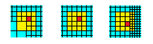
Figure 1. Each of the above illustrations depicts a cube $R$, coloured in red, contained in the grid $\Delta^{\gamma}_{0}$ in dimension two. The near region, $N(R)$, consists of all cubes highlighted in yellow together with the cube $R$. The far region, $F(R)$, is coloured blue and extends out to infinity.

As our operator is expected to behave differently at large scales than at local scales, it is desirable to split it up into local and non-local components. For any sub-linear operator $B$, define

$$B_{loc}f(x):=B\left(f\cdot\chi_{N(R_{x})}\right)(x)\quad\mathrm{and}$$

$$B_{far}f(x):=B\left(f\cdot\chi_{F(R_{x})}\right)(x),\quad\phantom{an}$$

for $f\in L^{1}_{loc}(\mathbb{R}^{d})$ and $x\in\mathbb{R}^{d}$. Notice that due to sub-linearity, for any weight $w$ on $\mathbb{R}^{d}$, to bound the quantity $\left\|Bf\right\|_{L^{p}(w)}$, it is both sufficient and necessary to bound $\left\|B_{loc}f\right\|_{L^{p}(w)}$ and $\left\|B_{far}f\right\|_{L^{p}(w)}$.

Now that sufficient preliminaries have been discussed, the details of our construction will be outlined. As noted previously, $\Delta^{\gamma}_{0}$ acts as a mediator between the local and non-local worlds. It is then appropriate to consider maximal functions of the below general form as candidates for an adapted maximal function for $\mathcal{L}$.

Definition 1.2.

For $Q\in\Delta$, let $\mathcal{G}(Q)$ be the collection of cubes

$$\mathcal{G}(Q):=\left\{\begin{array}[]{c c}\left\{Q\right\}&\mathrm{if}\ Q\in\Delta^{\gamma}_{0}\\ \left\{R^{\prime}\in\Delta^{\gamma}_{0}:R^{\prime}\subset Q\right\}&\mathrm{otherwise}.\end{array}\right.$$

Then for $c:\Delta\times\Delta^{\gamma}_{0}\times\Delta^{\gamma}_{0}\rightarrow\mathbb{R}_{\geq 0}$, $f\in L^{1}_{loc}(\mathbb{R}^{d})$ and $x\in R\in\Delta^{\gamma}_{0}$, define the operator $\mathcal{M}_{c}$ by

(2) $$\mathcal{M}_{c}f(x):=\sup_{Q\in\Delta,\ Q\ni x}\frac{1}{\left|Q\right|}\sum_{R^{\prime}\in\mathcal{G}(Q)}c(Q,R,R^{\prime})\int_{R^{\prime}}\left|f(y)\right|dy.$$

Notice that if $c(Q,R,R^{\prime})=1$ for all $R^{\prime}\in\mathcal{G}(Q)$ and $Q\in\Delta$, then the operator $\mathcal{M}_{c}$ is identical to the classical dyadic Hardy-Littlewood operator.

This looks promising but how do we determine what the right $c$-coefficients are? Any candidate for an adapted Hardy-Littlewood should share similar properties to the classic Hardy-Littlewood. We will determine appropriate coefficients from one of these properties. Let $M$ and $T^{*}$ denote the classical Hardy-Littlewood and heat maximal operator respectively. That is,

$$Mf(x):=\sup_{Q\ \mathrm{cube},\ Q\ni x}\frac{1}{\left|Q\right|}\int_{Q}\left|f(y)\right|dy\qquad\mathrm{and}\qquad T^{*}f(x):=\sup_{t>0}e^{t\Delta}\left|f\right|(x),$$

for $f\in L^{1}_{loc}(\mathbb{R}^{d})$ and $x\in\mathbb{R}^{d}$. Also recall that the $A_{p}$ class of weights is defined to be the collection of all weights, $w$ on $\mathbb{R}^{d}$, for which there exists a constant $C>0$ that satisfies

$$w(Q)^{\frac{1}{p}}\cdot w^{-\frac{1}{p-1}}(Q)^{\frac{p-1}{p}}\leq C\left|Q\right|$$

for all cubes $Q$ in $\mathbb{R}^{d}$. The following theorem is a well-known result from weighted theory.

Theorem 1.1.

Let $w$ be a weight on $\mathbb{R}^{d}$ and $1<p<\infty$. Then

$$w\in A_{p}\quad\Leftrightarrow\quad\left\|M\right\|_{L^{p}(w)\rightarrow L^{p}(w)}<\infty\quad\Leftrightarrow\quad\left\|T^{*}\right\|_{L^{p}(w)\rightarrow L^{p}(w)}<\infty.$$

Refer to [Ste16] sections V.4 and V.6 for proof. The above theorem indicates that if we are to construct a Hardy-Littlewood type maximal operator for $\mathcal{L}$, then the correct $c$-coefficients should satisfy the below equivalence for each $1<p<\infty$,

$$\left\|\mathcal{T}^{*}\right\|_{L^{p}(w)\rightarrow L^{p}(w)}<\infty\quad\Leftrightarrow\quad\left\|\mathcal{M}_{c}\right\|_{L^{p}(w)\rightarrow L^{p}(w)}<\infty,$$

where $\mathcal{T}^{*}$ is the semigroup maximal operator associated to $\mathcal{L}$,

$$\mathcal{T}^{*}f(x):=\sup_{t>0}e^{-t\mathcal{L}}\left|f\right|(x).$$

The coefficients for our generalised maximal function will be optimised in an attempt to produce the above equivalence.

A significant source of inspiration for this investigation stemmed from [BHS11]. In this paper, Bongioanni, Harboure and Salinas defined a new class of weights, $A_{p}^{\infty}$, for which $\mathcal{T}^{*}$ was bounded on $L^{p}(w)$ for all weights $w\in A_{p}^{\infty}$. What was interesting about this class was that it was strictly larger than the classic Muckenhoupt class. It seems that by including the potential $\left|x\right|^{2}$, the weight class $A_{p}$ effectively increases in size. It can be inferred from this, that in order to produce a maximal function smaller than $M$ and therefore a larger weight class, the coefficients for our maximal function must be smaller than unity. The $A_{p}^{\infty}$ class is defined to be $A_{p}^{\infty}:=\cup_{\theta\geq 0}A_{p}^{\theta}$, where $w\in A_{p}^{\theta}$ if and only if there exists some constant $C>0$ such that for all cubes $Q\subset\mathbb{R}^{d}$,

$$w(Q)^{1/p}w^{-\frac{1}{p-1}}(Q)^{\frac{p-1}{p}}\leq C\left|Q\right|\left(1+\frac{l(Q)}{\rho(c_{Q})}\right)^{\theta}.$$

In [Tan15], the author developed a maximal function $M^{\theta}$ adapted to the class $A_{p}^{\theta}$ in the sense that $M^{\theta}:L^{p}(w)\rightarrow L^{p}(w)$ is bounded if and only if $w\in A_{p}^{\theta}$. This operator is defined through

(3) $$M^{\theta}f(x):=\sup_{Q\ni x}\frac{1}{\psi_{\theta}(Q)\left|Q\right|}\int_{Q}\left|f(y)\right|dy,$$

where

$$\psi_{\theta}(Q):=\left(1+\frac{l(Q)}{\rho(c_{Q})}\right)^{\theta}.$$

Notice that this maximal function is also an example of the general class from definition 1.2 with $c(Q,R,R^{\prime})=\psi_{\theta}(Q)^{-1}<1$. This allows for more weights in the class $A_{p}^{\theta}$. However, it does not take into account the fact that if the cubes $R$ and $R^{\prime}$ are far apart, then the potential should have a larger effect and therefore the coefficient $c(Q,R,R^{\prime})$ should be smaller. The coefficients that we define for our maximal function take this into account. The main theorem of this paper is stated below.

Theorem A.

There exists maximal functions, $\mathcal{M}^{-}_{far}$ and $\mathcal{M}^{+}_{far}$, of similar form to definition 1.2 that satisfy the chain of implications

$$\left\|\mathcal{M}^{+}_{far}\right\|_{L^{p}(w)}<\infty\quad\Rightarrow\quad\left\|\mathcal{T}^{*}_{far}\right\|_{L^{p}(w)}<\infty\quad\Rightarrow\quad\left\|\mathcal{M}^{-}_{far}\right\|_{L^{p}(w)}<\infty,$$

for any weight $w$ on $\mathbb{R}^{d}$ and $1<p<\infty$.

For a precise definition of the above maximal functions, $\mathcal{M}^{-}_{far}$ and $\mathcal{M}^{+}_{far}$, and a proof of this statement, refer to section 3. A secondary result of this paper that characterises the local behaviour of an adapted maximal function is stated below.

Theorem B.

For any weight $w$ on $\mathbb{R}^{d}$ and $1<p<\infty$,

$$\left\|M_{loc}\right\|_{L^{p}(w)\rightarrow L^{p}(w)}<\infty\quad\Leftrightarrow\quad\left\|\mathcal{T}^{*}_{loc}\right\|_{L^{p}(w)\rightarrow L^{p}(w)}<\infty.$$

This theorem will be proved in section 2. Together, these two statements demonstrate that for any weight in the class

$$A_{p}^{+}:=\left\{w\ \mathrm{weight}\ \mathrm{on}\ \mathbb{R}^{d}:\left\|\mathcal{M}^{+}_{far}\right\|_{L^{p}(w)\rightarrow L^{p}(w)}<\infty\ \mathrm{and}\ \left\|M_{loc}\right\|_{L^{p}(w)\rightarrow L^{p}(w)}<\infty\right\},$$

we have $\left\|\mathcal{T}^{*}\right\|_{L^{p}(w)\rightarrow L^{p}(w)}<\infty$.

It is then natural to ask how our weight class compares with the class $A_{p}^{\infty}$? Section 4 provides an answer to this question in the form of the following proposition.

Proposition C.

The following chain of strict inclusions holds for any $1<p<\infty$,

$$A_{p}\subsetneq A_{p}^{\infty}\subsetneq A_{p}^{+}.$$

The above inclusion indicates that our coefficients serve as an improvement upon the constant coefficients of (3).

Finally, in section 5, the techniques developed throughout this paper will be used to show that the heat maximal operator for $\mathcal{L}$ can be safely truncated when considering weighted questions.

This paper is part of my PhD thesis, supervised by Pierre Portal at the Australian National University. It is inspired by discussions of my supervisor with Paco Villarroya, aiming to understand better how to adapt harmonic analysis to the hidden geometry of a differential operator. In most cases, this involves situations beyond the reach of Calderón-Zygmund theory (see e.g. [MM07, HM09]). However, this can also be done within Calderón-Zygmund theory by proving stronger properties of smaller classes of singular integral operators than the Calderón-Zygmund class. Paco Villaroya has particularly focused on describing compact (as opposed to merely bounded) singular integral operators (see e.g. [Vil15]). To do so, he had to refine classical dyadic approaches, in order to understand which cubes particularly affect compactness. I follow a similar path here, modifying standard dyadic arguments in a way that aims to reveal the “hidden geometry” of the harmonic oscillator. This is done by attempting to find the largest class of weights for which the corresponding heat maximal operator is bounded. Perhaps surprisingly, such a question seems to be rarely formulated in the context of standard weighted Calderón-Zygmund theory (generic questions involving all singular integrals and all related maximal functions are considered instead), but quite common in the context of two weights inequalities (where studying just the Hilbert transform is hard enough, and natural).

I would like to thank the anonymous referee of a previous version of this paper for their suggestion that the proof of the inclusion $A_{p}^{\infty}\subseteq A_{p}^{+}$ should be made strict.

2. The Local Class

In this section, a local version of the $A_{p}$ class is introduced, $A_{p}^{loc}$. This class is a dyadic variation of a similar class introduced in [BHS11]. Through this class, and a few preliminary lemmas, Theorem B will be proved.

Consider a cube in $\mathbb{R}^{d}$, $Q_{0}:=[a_{1},a_{1}+l(Q_{0}))\times\cdots\times[a_{d},a_{d}+l(Q_{0}))$, where $\left\{a_{1},\cdots,a_{d}\right\}\subset\mathbb{R}$. In the usual manner, this cube can be divided into $2^{d}$ congruent disjoint cubes with half the side-length of the original cube. These cubes can themselves be divided into $2^{d}$ disjoint cubes each and so on ad infinitum. If a cube $Q\subset\mathbb{R}^{d}$ can be obtained in this manner from $Q_{0}$, then it is called a dyadic subcube of the cube $Q_{0}$. Note that we did not require our initial cube $Q_{0}$ to be a member of the standard dyadic grid and that $Q_{0}$ is a dyadic subcube of itself.

Definition 2.1.

Fix a weight $w$ on $\mathbb{R}^{d}$ and $1<p<\infty$. For a cube $Q_{0}\subset\mathbb{R}^{d}$, the weight $w$ is said to belong to the class $A_{p}(Q_{0})$ if there exists a constant $C>0$ such that

(4) $$w^{-\frac{1}{p-1}}(Q)^{\frac{p-1}{p}}w(Q)^{\frac{1}{p}}\leq C\left|Q\right|$$

for all dyadic subcubes $Q\subseteq Q_{0}$. The smallest such $C$ is denoted $\left[w\right]_{A_{p}(Q_{0})}$.

A variation of the next statement was originally proved in [Har84]. It is an extension lemma for weights that satisfy the $A_{p}$ property when restricted to a cube.

Lemma 2.1.

Fix a cube $Q_{0}\subset\mathbb{R}^{d}$, $1<p<\infty$ and a weight $w\in A_{p}(Q_{0})$. Then there exists a weight $w_{Q_{0}}\in A_{p}(\mathbb{R}^{d})$ that coincides with $w$ on $Q_{0}$ such that $\left[w_{Q_{0}}\right]_{A_{p}}=\left[w\right]_{A_{p}(Q_{0})}$.

Proof.

Our proof proceeds by construction. Let $\mathcal{D}^{Q_{0}}$ denote a dyadic system of cubes on $\mathbb{R}^{d}$ for which $Q_{0}$ is a member. This can be explicitly constructed as follows. First, scale the standard dyadic grid by a factor of $l(Q_{0})$ to form the collection $l(Q_{0})\cdot\Delta$ that consists of all cubes of the form

$$\left[m_{1}2^{k}l(Q_{0}),\left(m_{1}+1\right)2^{k}l(Q_{0})\right)\times\cdots\times\left[m_{d}2^{k}l(Q_{0}),\left(m_{d}+1\right)2^{k}l(Q_{0})\right)$$

where $k,m_{1},\cdots,m_{d}\in\mathbb{Z}$. Then, if we let $b_{Q_{0}}$ denote the corner of the cube $Q_{0}$ closest to the origin, we can translate this scaled grid to $Q_{0}$,

$$\mathcal{D}^{Q_{0}}:=l(Q)\cdot\Delta+b_{Q_{0}}:=\left\{Q+b_{Q_{0}}:Q\in l(Q)\cdot\Delta\right\}.$$

Let $\mathcal{D}^{Q_{0}}_{0}$ denote the subcollection that consists of all cubes in $\mathcal{D}^{Q_{0}}$ of the same size as $Q_{0}$. A weight, $w_{Q_{0}}$ on $\mathbb{R}^{d}$, will be constructed for which there exists $B>0$ such that

(5) $$w_{Q_{0}}^{-\frac{1}{p-1}}(Q)^{\frac{p-1}{p}}w_{Q_{0}}(Q)^{\frac{1}{p}}\leq B\left|Q\right|$$

for all $Q\in\mathcal{D}^{Q_{0}}$. As the dyadic description of $A_{p}(\mathbb{R}^{d})$ is scale and translation invariant, this criteria will be sufficient to determine that $w_{Q_{0}}\in A_{p}(\mathbb{R}^{d})$.

Fix $Q\in\mathcal{D}^{Q_{0}}_{0}$. Let $\varphi_{Q}:\mathbb{R}^{d}\rightarrow\mathbb{R}^{d}$ denote the translation that takes the cube $Q$ to the cube $Q_{0}$. Then, for $x\in Q$, define

$$w_{Q_{0}}(x):=w\left(\varphi_{Q}(x)\right).$$

As the cubes in $\mathcal{D}^{Q_{0}}_{0}$ partition $\mathbb{R}^{d}$, this description defines a unique function $w_{Q_{0}}$ on $\mathbb{R}^{d}$. Moreover, it is clear that this function will be a weight that coincides with $w$ on $Q_{0}$.

By definition, as $w\in A_{p}(Q_{0})$, it follows that there must exist a $C>0$ such that (5) is satisfied for all dyadic subcubes $Q\subset Q_{0}$. Fix a cube $Q\in\mathcal{D}^{Q_{0}}$. Suppose that $Q$ is a dyadic subcube of a cube from $\mathcal{D}^{Q_{0}}_{0}$. Then (5) must be satisfied automatically with constant $C$. So suppose that $Q$ is not a dyadic subcube of any cube in $\mathcal{D}^{Q_{0}}_{0}$. Then, since a parent cube is always decomposable into its children, there must exist finitely many cubes $\left\{Q_{i}\right\}_{i=1}^{N}\subset\mathcal{D}^{Q_{0}}_{0}$ such that $Q=\sqcup_{i=1}^{N}Q_{i}$. We then have

$$\begin{split}w_{Q_{0}}^{-\frac{1}{p-1}}(Q)^{\frac{p-1}{p}}w_{Q_{0}}(Q)^{\frac{1}{p}}&=\left(\int_{Q}w_{Q_{0}}(y)^{-\frac{1}{p-1}}dy\right)^{\frac{p-1}{p}}\left(\int_{Q}w_{Q_{0}}(y)dy\right)^{\frac{1}{p}}\\ &=\left(\sum_{i=1}^{N}\int_{Q_{i}}w_{Q_{0}}(y)^{-\frac{1}{p-1}}dy\right)^{\frac{p-1}{p}}\left(\sum_{i=1}^{N}\int_{Q_{i}}w_{Q_{0}}(y)dy\right)^{\frac{1}{p}}\\ &=\left(N\int_{Q_{0}}w^{-\frac{1}{p-1}}(y)dy\right)^{\frac{p-1}{p}}\left(N\int_{Q_{0}}w(y)dy\right)^{\frac{1}{p}}\\ &\leq CN\left|Q_{0}\right|\\ &=C\left|Q\right|.\end{split}$$

∎

Definition 2.2.

Fix $1<p<\infty$. A weight $w$ on $\mathbb{R}^{d}$ is said to be in the class $A_{p}^{loc}$ if there exists a constant $C>0$ such that

$$\left[w\right]_{A_{p}(N(R))}\leq C$$

for all $R\in\Delta^{\gamma}_{0}$. The smallest such constant will be denoted by $\left[w\right]_{A_{p}^{loc}}$.

The subsequent lemma will be used numerous times throughout this investigation. It states the exact form of the heat kernel corresponding to $\mathcal{L}$. Its proof can be found in [Sim79] in dimension $1$. Higher dimensions follow from this case by taking tensor products of Hermite functions.

Lemma 2.2.

For $t>0$, define the map $k_{t}:\mathbb{R}^{d}\times\mathbb{R}^{d}\rightarrow\mathbb{R}$ through

(6) $$k_{t}(x,y)=h_{t}(x,y)\cdot\exp\left(-\alpha(t)\left(\left|x\right|^{2}+\left|y\right|^{2}\right)\right),$$

where $h_{t}$ is the classic heat kernel

$$h_{t}(x,y):=\frac{1}{\left(2\pi t\right)^{d/2}}\exp\left(-\frac{\left|x-y\right|^{2}}{2t}\right)$$

and $\alpha$ is defined by

$$\alpha(t):=\frac{\sqrt{1+t^{2}}-1}{2t}$$

for all $x$ and $y$ in $\mathbb{R}^{d}$. The operator $\mathcal{T}^{*}$ is then given by

$$\mathcal{T}^{*}f(x):=\sup_{t>0}\int_{\mathbb{R}^{d}}k_{t}(x,y)\left|f(y)\right|dy$$

for any $f\in L^{1}_{loc}(\mathbb{R}^{d})$ and $x\in\mathbb{R}^{d}$.

Note that the fundamental solution for $\mathcal{L}$ is actually $k_{\sinh 2t}$. We have chosen to rescale the kernel for simplicity. An expanded version of theorem B is presented and proved below.

Theorem B.

Let $T^{*}$ and $M$ denote the classic heat maximal operator and Hardy-Littlewood operator respectively. Let $w$ be a weight on $\mathbb{R}^{d}$. For any $1<p<\infty$, the following statements are equivalent.

1. $\left\|M_{loc}\right\|_{L^{p}(w)\rightarrow L^{p}(w)}<\infty$.
   

2. $w\in A_{p}^{loc}$.
   

3. $\left\|T^{*}_{loc}\right\|_{L^{p}(w)\rightarrow L^{p}(w)}<\infty$.
   

4. $\left\|\mathcal{T}^{*}_{loc}\right\|_{L^{p}(w)\rightarrow L^{p}(w)}<\infty$.

Proof.

We will prove the following chain of implications $(1)\Rightarrow(2)\Rightarrow(3)\Rightarrow(4)\Rightarrow(1)$.

$(1)\Rightarrow(2)$. Fix a cube $R\in\Delta^{\gamma}_{0}$, $Q$ a dyadic subcube of $N(R)$ and $f\in L^{1}_{loc}(\mathbb{R}^{d})$. Define $C:=\left\|M_{loc}\right\|_{L^{p}(w)\rightarrow L^{p}(w)}$. Then, using standard techniques from weighted theory,

$$\begin{split}\left(\int_{Q}w\right)\left(\frac{1}{\left|Q\right|}\int_{Q}\left|f\right|\right)^{p}&=\int_{Q}\left(\frac{1}{\left|Q\right|}\int_{Q}\left|f\right|\right)^{p}w(y)dy\\ &\leq\int_{Q}M_{loc}(f\cdot\chi_{Q})(y)^{p}w(y)dy\\ &\leq\left\|M_{loc}(f\cdot\chi_{Q})\right\|^{p}_{L^{p}(\mathbb{R}^{n},w)}\\ &\leq C^{p}\left\|f\cdot\chi_{Q}\right\|^{p}_{L^{p}(w)}\\ &=C^{p}\left(\int_{Q}\left|f\right|^{p}w\right).\end{split}$$

Take $f:=\left(w+\varepsilon\right)^{-\frac{1}{p-1}}$ for some $\varepsilon>0$. Then

$$w(Q)\left(\frac{1}{\left|Q\right|}\int_{Q}\left(w(y)+\varepsilon\right)^{-\frac{1}{p-1}}dy\right)^{p}\leq C^{p}\int_{Q}\frac{w(y)}{\left(w(y)+\varepsilon\right)^{\frac{p}{p-1}}}dy,$$

which implies that

$$w(Q)\left(\int_{Q}\left(w(y)+\varepsilon\right)^{-\frac{1}{p-1}}dy\right)^{p}\leq C^{p}\left|Q\right|^{p}\int_{Q}\frac{\left(w(y)+\varepsilon\right)}{\left(w(y)+\varepsilon\right)^{\frac{p}{p-1}}}dy,$$

$$\Rightarrow w(Q)\left(\int_{Q}\left(w(y)+\varepsilon\right)^{-\frac{1}{p-1}}dy\right)^{p-1}\leq C^{p}\left|Q\right|^{p}$$

for each $\varepsilon>0$. An application of the Lebesgue monotone convergence theorem then produces the desired result.

$(2)\Rightarrow(3)$. Lemma 2.1 states that for any cube $R\in\Delta^{\gamma}_{0}$ the restriction $w|_{N(R)}$ can be extended to an $A_{p}$ weight $w_{N(R)}$. As $w_{N(R)}\in A_{p}$, we know from classical theory that $\left\|T^{*}\right\|_{L^{p}(w_{N(R)})\rightarrow L^{p}(w_{N(R)})}\lesssim\left[w_{N(R)}\right]_{A_{p}}<\infty$. Then, for $f\in L^{p}(w)$,

$$\begin{split}\left\|T_{loc}^{*}f\right\|^{p}_{L^{p}(w)}&=\int_{\mathbb{R}^{d}}T_{loc}^{*}f(x)^{p}w(x)dx\\ &=\sum_{R\in\Delta^{\gamma}_{0}}\int_{R}T^{*}(f\cdot\chi_{N(R)})(x)^{p}w(x)dx\\ &\leq\sum_{R\in\Delta^{\gamma}_{0}}\int_{\mathbb{R}^{d}}T^{*}(f\cdot\chi_{N(R)})(x)^{p}w_{N(R)}(x)dx\\ &\lesssim\sum_{R\in\Delta^{\gamma}_{0}}\left[w_{N(R)}\right]_{A_{p}}^{p}\int_{N(R)}\left|f(x)\right|^{p}w_{N(R)}(x)dx\\ &\leq\left[w\right]_{A_{p}^{loc}}^{p}\sum_{R\in\Delta^{\gamma}_{0}}\int_{N(R)}\left|f(x)\right|^{p}w(x)dx\\ &\lesssim\left[w\right]_{A_{p}^{loc}}^{p}\int_{\mathbb{R}^{d}}\left|f(x)\right|^{p}w(x)dx,\end{split}$$

where the final inequality was obtained from the bounded overlap property of the cubes $\left\{N(R)\right\}_{R\in\Delta^{\gamma}_{0}}$.

$(3)\Rightarrow(4)$. This follows trivially from the inequality $k_{t}(x,y)\leq h_{t}(x,y)$ for all $x,y\in\mathbb{R}^{d}$ and $t>0$.

$(4)\Rightarrow(1)$. Fix $f\in L^{1}_{loc}(\mathbb{R}^{d})$ and $x\in R\in\Delta^{\gamma}_{0}$. Let $Q$ be any cube containing $x$ that satisfies $Q\subseteq N(R)$. We first observe that for any $y\in Q$,

$$\exp(-\frac{\left|x-y\right|^{2}}{2l(Q)^{2}})\approx 1.$$

To see this, note that

$$\left|x-y\right|\leq\sqrt{d}l(Q).$$

This implies that

$$-\frac{\left|x-y\right|^{2}}{2l(Q)^{2}}\geq-\frac{d}{2},$$

and therefore

$$\exp(-\frac{\left|x-y\right|^{2}}{2l(Q)^{2}})\gtrsim 1.$$

Moreover, we trivially have

$$\exp(-\frac{\left|x-y\right|^{2}}{2l(Q)^{2}})\leq 1.$$

Note that for any $x,y\in Q$, since $l(Q)\leq 4l(R)$, we have the bound

$$\begin{split}\left|x\right|,\left|y\right|&\leq 2\sqrt{d}2^{j(R)}\\ &=\frac{2\sqrt{d}}{l(R)}\\ &\leq\frac{8\sqrt{d}}{l(Q)}.\end{split}$$

This then implies that

$$\begin{split}\exp\left(-\frac{\left(\sqrt{1+l(Q)^{4}}-1\right)}{2l(Q)^{2}}\left(\left|x\right|^{2}+\left|y\right|^{2}\right)\right)\geq\exp\left(-\frac{8^{2}d\left(\sqrt{1+l(Q)^{4}}-1\right)}{l(Q)^{4}}\right).\end{split}$$

It is easy to show that the bound

$$\frac{\sqrt{1+t^{4}}-1}{t^{4}}\leq\frac{1}{2}$$

is satisfied for all $t>0$. This then gives us

$$\exp\left(-\frac{\left(\sqrt{1+l(Q)^{4}}-1\right)}{2l(Q)^{2}}\left(\left|x\right|^{2}+\left|y\right|^{2}\right)\right)\geq e^{-\frac{8^{2}d}{2}}.$$

For $t:=l(Q)^{2}$, we then have

$$\begin{split}\frac{1}{\left|Q\right|}\int_{Q}&\left|f(y)\right|dy\\ &\lesssim\frac{1}{l(Q)^{d}}\int_{Q}\exp\left(-\frac{\left(\sqrt{1+l(Q)^{4}}-1\right)}{2l(Q)^{2}}\left(\left|x\right|^{2}+\left|y\right|^{2}\right)\right)\exp\left(-\frac{\left|x-y\right|^{2}}{2l(Q)^{2}}\right)\left|f(y)\right|dy\\ &=\int_{Q}\frac{1}{t^{d/2}}\exp\left(-\frac{\left(\sqrt{1+t^{2}}-1\right)}{2t}\left(\left|x\right|^{2}+\left|y\right|^{2}\right)\right)\exp\left(-\frac{\left|x-y\right|^{2}}{2t}\right)\left|f(y)\right|dy\\ &\lesssim\int_{Q}k_{t}(x,y)\left|f(y)\right|dy\\ &\lesssim\mathcal{T}^{*}_{loc}f(x).\end{split}$$

On taking the supremum over all such $Q$, we obtain $M_{loc}f(x)\lesssim\mathcal{T}^{*}_{loc}f(x)$. ∎

3. The Far Class

In this section, the adapted operators $\mathcal{M}^{-}_{far}$ and $\mathcal{M}^{+}_{far}$ are defined and theorem A is proved. With this, a sufficient condition for the boundedness of $\left\|\mathcal{T}^{*}\right\|_{L^{p}(w)\rightarrow L^{p}(w)}$ is obtained. Prior to presenting these definitions, it is necessary to introduce a collection of cubes that represent the regions over which our averaging operators will act.

Definition 3.1.

For each $R\in\Delta^{\gamma}_{0}$, define the following subsets of $\mathbb{R}^{d}$.

1. $Q_{0}(R)$ is the smallest cube containing the region

   $$\left\{y\in\mathbb{R}^{d}:\left|y\right|\leq 2^{16}d^{4}2^{j(R)}\right\},$$

   that can be decomposed into cubes from the grid $\Delta^{\gamma}_{0}$.

2. For $t\leq 2^{4}d^{2}$, $Q_{t}(R):=Q_{0}(R)$.

3. For $t\geq 2^{4}d^{2}$, $Q_{t}(R)$ is the smallest cube containing the region

   $$\left\{y\in\mathbb{R}^{d}:\left|y\right|\leq 2^{8}t^{2}2^{j(R)}\right\},$$

   that can be decomposed into cubes from the grid $\Delta^{\gamma}_{0}$.

For sets $A$ and $B$ contained in $\mathbb{R}^{d}$, introduce the notation $k_{t}^{+}(A,B)$ and $k_{t}^{-}(A,B)$ to denote respectively the supremum and infimum of $k_{t}(x,y)$ over all $x\in A$ and $y\in B$.

Definition 3.2.

For $f\in L^{1}_{loc}(\mathbb{R}^{d})$ and $x\in R\in\Delta^{\gamma}_{0}$, define the operators $\mathcal{M}^{+}_{far}$ and $\mathcal{M}^{-}_{far}$ through

(7) $$\begin{split}&\mathcal{M}^{+}_{far}f(x):=\sup_{t>0}\sum_{R^{\prime}\in\mathcal{F}(R),\ R^{\prime}\subset Q_{t}(R)}k_{t}^{+}(R,R^{\prime})\int_{R^{\prime}}\left|f(y)\right|dy,\qquad\mathrm{and}\\ \phantom{c}\\ &\mathcal{M}^{-}_{far}f(x):=\sup_{t>0}\sum_{R^{\prime}\in\mathcal{F}(R),\ R^{\prime}\subset Q_{t}(R)}k_{t}^{-}(R,R^{\prime})\int_{R^{\prime}}\left|f(y)\right|dy.\end{split}$$

With the introduction of our maximal functions, it is a straightforward matter to define their corresponding weight classes.

Definition 3.3.

For $1<p<\infty$, the classes of weights on $\mathbb{R}^{d}$, $A_{p}^{far+}$ and $A_{p}^{far-}$, are defined through

(8) $$\begin{split}&A_{p}^{far+}:=\left\{w\ \mathrm{weight}\ \mathrm{on}\ \mathbb{R}^{d}:\left\|\mathcal{M}^{+}_{far}\right\|_{L^{p}(w)\rightarrow L^{p}(w)}<\infty\right\}\quad\mathrm{and}\\ \phantom{c}\\ &A_{p}^{far-}:=\left\{w\ \mathrm{weight}\ \mathrm{on}\ \mathbb{R}^{d}:\left\|\mathcal{M}^{-}_{far}\right\|_{L^{p}(w)\rightarrow L^{p}(w)}<\infty\right\}.\end{split}$$

We then define $A_{p}^{+}:=A_{p}^{far+}\cap A_{p}^{loc}$ and $A_{p}^{-}:=A_{p}^{far-}\cap A_{p}^{loc}$.

In order to verify our main result, a string of technical lemmas must first be proved. The first two of these provide some valuable estimates concerning the maximum of the function $t\mapsto k_{t}(x,y)$ for fixed $x$ and $y$ in $\mathbb{R}^{d}$.

Lemma 3.1.

Fix points $x\in R\in\Delta^{\gamma}_{0}$ and $y\notin Q_{0}(R)$. There is precisely one maximum for the function $t\mapsto k_{t}(x,y)$. Denote this point by $t_{m}(x,y)$. Then for $R$ not contained in the first layer, $t_{m}(x,y)$ must satisfy

(9) $$\frac{\left|y\right|}{9\cdot d\left|x\right|}\leq t_{m}(x,y)\leq\frac{\left|x-y\right|^{2}}{d}.$$

For $R$ contained in the first layer, $t_{m}(x,y)$ will satisfy

(10) $$\frac{\left|y\right|}{9\cdot d}\leq t_{m}(x,y)\leq\frac{\left|x-y\right|^{2}}{d}.$$

Proof.

On differentiating expression (6) with respect to $t$ we obtain

$$\dfrac{\partial}{\partial t}k_{t}(x,y)=\frac{1}{2t^{2}}g(t)k_{t}(x,y),$$

where the function $g$ is defined to be

$$g(t):=-d\cdot t+\frac{\left(\left|x\right|^{2}+\left|y\right|^{2}\right)}{\sqrt{1+t^{2}}}-2\langle x,y\rangle.$$

As the kernel $k_{t}(x,y)$ is always positive, it follows that the sign of the derivative will be identical to the sign of the function $g(t)$. Suppose that $g$ is negative. Then we must have

$$\left(d\cdot t+2\langle x,y\rangle\right)\sqrt{1+t^{2}}>\left(\left|x\right|^{2}+\left|y\right|^{2}\right)$$

That is, the derivative of the kernel will be negative if and only if the above inequality holds. Likewise, the derivative of the kernel will be positive if and only if

(11) $$\left(d\cdot t+2\langle x,y\rangle\right)\sqrt{1+t^{2}}<\left(\left|x\right|^{2}+\left|y\right|^{2}\right)$$

and the derivative will vanish if and only if equality holds.

It is simple to show that $\left|x-y\right|^{2}/d$ serves as the only maximum of the function $t\mapsto h_{t}(x,y)$. This implies that $h_{t}(x,y)$ is decreasing for $t>\left|x-y\right|^{2}/d$. As the function $\alpha(t)$ is strictly increasing, we have that

$$\exp\left(-\alpha(t)\left(\left|x\right|^{2}+\left|y\right|^{2}\right)\right)$$

is strictly decreasing for all $t$. This shows that $k_{t}(x,y)$ is strictly decreasing for $t>\left|x-y\right|^{2}/d$. It then follows that any maximum for $t\mapsto k_{t}(x,y)$ must be less than $\left|x-y\right|^{2}/d$. As this function must approach $0$ as $t$ approaches $0$, continuity of the derivative then implies that there must exist at least one maximum in the interval $\left[0,\left|x-y\right|^{2}/d\right]$.

Let $t_{m}(x,y)$ denote the largest maximum in the above interval. It will be shown that $t_{m}(x,y)$ is the only maximum. From our previous argument, equality will hold in (11) for the value $t_{m}(x,y)$. Suppose that $t_{0}<t_{m}(x,y)$. Then $t_{0}=t_{m}(x,y)-a$ for some $a>0$. We then have

$$\begin{split}\left(d\cdot t_{0}+2\langle x,y\rangle\right)\sqrt{1+t_{0}^{2}}&=\left(d\cdot t_{m}(x,y)-d\cdot a+2\langle x,y\rangle\right)\sqrt{1+t_{0}^{2}}\\ &=\left(d\cdot t_{m}(x,y)+2\langle x,y\rangle\right)\sqrt{1+t_{0}^{2}}-d\cdot a\sqrt{1+t_{0}^{2}}.\end{split}$$

As equality holds in expression (11) for $t_{m}(x,y)$, it follows that the factor $\left(d\cdot t_{m}(x,y)\right)+2\langle x,y\rangle$ must be positive. Therefore

$$\begin{split}\left(d\cdot t_{0}+2\langle x,y\rangle\right)\sqrt{1+t_{0}^{2}}&\leq\left(d\cdot t_{m}(x,y)+2\langle x,y\rangle\right)\sqrt{1+t_{m}(x,y)^{2}}-d\cdot a\sqrt{1+t_{0}^{2}}\\ &=\left(\left|x\right|^{2}+\left|y\right|^{2}\right)-d\cdot a\sqrt{1+t_{0}^{2}}\\ &<\left(\left|x\right|^{2}+\left|y\right|^{2}\right).\end{split}$$

This demonstrates that the derivative must be positive for any $t_{0}<t_{m}(x,y)$.

Let’s now show the lower bound for $t_{m}(x,y)$. First suppose that $R$ is not contained in the first layer. It will be shown that for any $t_{1}<\left|y\right|/\left(9\cdot d\left|x\right|\right)$, inequality (11) holds. From our previous argument, this will then imply that the function is increasing on the interval $\left[0,\left|y\right|/\left(9\cdot d\left|x\right|\right)\right)$. As $y\notin Q_{0}(R)$, it follows that $y$ satisfies the bound $\left|y\right|>3\left|x\right|$. We know that

$$\begin{split}1+t_{1}^{2}&<1+\frac{1}{9}\left(\frac{\left|y\right|}{3\left|x\right|}\right)^{2}\\ &=1+\left(\frac{\left|y\right|}{3\left|x\right|}\right)^{2}-\frac{8}{9}\left(\frac{\left|y\right|}{3\left|x\right|}\right)^{2}\\ &\leq 1+\left(\frac{\left|y\right|}{3\left|x\right|}\right)^{2}-\frac{8}{9}\\ &=\frac{1}{9}\left(1+\frac{\left|y\right|^{2}}{\left|x\right|^{2}}\right).\end{split}$$

We also have

$$\begin{split}\left(d\cdot t_{1}+2\langle x,y\rangle\right)&\leq\left(d\cdot t_{1}+2\left|\langle x,y\rangle\right|\right)\\ &\leq\left(\frac{\left|y\right|}{9\left|x\right|}+2\left|x\right|\left|y\right|\right)\\ &\leq\left(\frac{\left|y\right|}{\left|x\right|}\right)\left(\frac{1}{9}+2\left|x\right|^{2}\right)\\ &\leq\left(\frac{\left|y\right|}{\left|x\right|}\right)3\left|x\right|^{2}.\end{split}$$

This demonstrates that

$$\begin{split}\left(d\cdot t_{1}+2\langle x,y\rangle\right)\sqrt{1+t_{1}^{2}}&<\left(3\left|x\right|\left|y\right|\right)\cdot\frac{1}{3}\sqrt{1+\frac{\left|y\right|^{2}}{\left|x\right|^{2}}}\\ &=\left|y\right|\sqrt{\left|x\right|^{2}+\left|y\right|^{2}}\\ &\leq\left(\left|x\right|^{2}+\left|y\right|^{2}\right).\end{split}$$

Now suppose that $R$ is in the first layer and $y\notin Q_{0}(R)$. Then $\left|y\right|\geq 2^{16}d^{4}$. Let $t_{2}<\left|y\right|/\left(9d\right)$. Then

$$\begin{split}\left(1+t_{2}^{2}\right)&<\left(1+\left(\frac{\left|y\right|}{9d}\right)^{2}\right)\\ &\leq\left(\frac{\left|y\right|^{2}}{2^{32}d^{8}}+\frac{\left|y\right|^{2}}{9^{2}d^{2}}\right)\\ &\leq\frac{2\left|y\right|^{2}}{9^{2}d^{2}}.\end{split}$$

On noting that $\left|x\right|\leq\sqrt{d}$,

$$\begin{split}\left(d\cdot t_{2}+2\langle x,y\rangle\right)&\leq\left(d\cdot t_{2}+2\left|\langle x,y\rangle\right|\right)\\ &\leq\left(\frac{\left|y\right|}{9}+2\left|x\right|\left|y\right|\right)\\ &\leq\left(\frac{1}{9}+2\left|x\right|\right)\left|y\right|\\ &\leq\left(\frac{1}{9}+2\sqrt{d}\right)\left|y\right|\\ &\leq 3\sqrt{d}\left|y\right|\end{split}$$

This finally leads to

$$\begin{split}\left(d\cdot t_{2}+2\langle x,y\rangle\right)\sqrt{1+t_{2}^{2}}&<\left(3\sqrt{d}\left|y\right|\right)\left(\frac{\sqrt{2}\left|y\right|}{9d}\right)\\ &\leq\left|y\right|^{2}\\ &\leq\left(\left|x\right|^{2}+\left|y\right|^{2}\right),\end{split}$$

which validates our lower bound. ∎

Lemma 3.2.

Fix cubes $R$ and $R^{\prime}$ in $\Delta^{\gamma}_{0}$ with $R^{\prime}\subset Q_{0}(R)^{c}$. Fix points $x\in R$ and $y\in R^{\prime}$. The maximum $t_{m}(x,y)$ satisfies the inequality,

(12) $$2\leq 8\cdot t_{m}(x,y)\sqrt{\frac{2^{j(R)+j(R^{\prime})}}{\left|x\right|^{2}+\left|y\right|^{2}}}\leq\frac{t_{m}(x,y)}{2^{4}d^{2}}.$$

Proof.

As $y\notin Q_{0}(R)$, we have $\left|y\right|\geq 2^{16}d^{4}2^{j(R)}$ and also $\left|y\right|\geq 2^{j(R^{\prime})-1}$. The upper inequality then follows from

$$\begin{split}\left|x\right|^{2}+\left|y\right|^{2}&\geq\left|y\right|^{2}\\ &\geq 2^{j(R^{\prime})-1}2^{16}d^{4}2^{j(R)}\\ &=2^{15}d^{4}2^{j(R)+j(R^{\prime})}.\end{split}$$

As for the lower bound, first consider when $R$ is not in the first layer. On applying Lemma 3.1 and recalling that $\left|y\right|\geq\left|x\right|$,

$$\begin{split}t_{m}(x,y)\sqrt{\frac{2^{j(R)+j(R^{\prime})}}{\left|x\right|^{2}+\left|y\right|^{2}}}&\geq\frac{\left|y\right|}{9d\left|x\right|}\sqrt{\frac{2^{j(R)+j(R^{\prime})}}{\left|x\right|^{2}+\left|y\right|^{2}}}\\ &\geq\frac{1}{9d}\sqrt{\frac{\left|y\right|^{2}2^{j(R)+j(R^{\prime})}}{2\left|x\right|^{2}\left|y\right|^{2}}}.\end{split}$$

Then on applying the bounds $\left|x\right|\leq\sqrt{d}2^{j(R)}$, $\left|y\right|\leq\sqrt{d}2^{j(R^{\prime})}$ and $\left|y\right|\geq 2^{16}d^{4}2^{j(R)}$ successively we obtain

$$\begin{split}t_{m}(x,y)\sqrt{\frac{2^{j(R)+j(R^{\prime})}}{\left|x\right|^{2}+\left|y\right|^{2}}}&\geq\frac{1}{9d}\sqrt{\frac{2^{j(R)+j(R^{\prime})}}{2d2^{2j(R)}}}\\ &\geq\frac{1}{9d}\sqrt{\frac{\left|y\right|}{2d^{3/2}2^{j(R)}}}\\ &\geq\frac{1}{9d}\sqrt{\frac{2^{16}d^{4}2^{j(R)}}{2d^{3/2}2^{j(R)}}}\\ &\geq 2.\end{split}$$

Next, consider when $R$ is in the first layer. Once again apply Lemma 3.1 and $\left|y\right|\geq\left|x\right|$ to obtain

$$\begin{split}t_{m}(x,y)\sqrt{\frac{2^{j(R)+j(R^{\prime})}}{\left|x\right|^{2}+\left|y\right|^{2}}}&\geq\frac{\left|y\right|}{9d}\sqrt{\frac{2^{j(R^{\prime})}}{2\left|y\right|^{2}}}\\ &=\frac{1}{9d}\sqrt{\frac{2^{j(R^{\prime})}}{2}}.\end{split}$$

Then, on successively applying the bounds $\left|y\right|\leq\sqrt{d}2^{j(R^{\prime})}$ and $\left|y\right|\geq 2^{16}d^{4}$,

$$\begin{split}t_{m}(x,y)\sqrt{\frac{2^{j(R)}+2^{j(R^{\prime})}}{\left|x\right|^{2}+\left|y\right|^{2}}}&\geq\frac{1}{9d}\sqrt{\frac{\left|y\right|}{2\sqrt{d}}}\\ &\geq\frac{1}{9d}\sqrt{\frac{2^{16}d^{4}}{2\sqrt{d}}}\\ &\geq 2.\end{split}$$

This concludes the proof. ∎

The next lemma obtains an estimate on ratios of the form $k_{t}(x,y)\cdot k_{t_{m}(x,y)}(x,y)^{-1}$ for fixed $x$ and $y$. It will play a key role in the proof of theorem A.

Lemma 3.3.

Fix cubes $R$ and $R^{\prime}$ in $\Delta^{\gamma}_{0}$ with $R^{\prime}\subset Q_{0}(R)^{c}$. Fix the points $x\in R$ and $y\in R^{\prime}$. Introduce the shorthand notation $t_{m}:=t_{m}(x,y)$. Define

$$M:=8\cdot t_{m}\sqrt{\frac{2^{j(R)+j(R^{\prime})}}{\left|x\right|^{2}+\left|y\right|^{2}}}.$$

Then we must have the bound

(13) $$k_{t}(x,y)\cdot k_{t_{m}}(x,y)^{-1}\lesssim\frac{1}{2^{(j(R)+j(R^{\prime}))(d+1)}}$$

for all $t\leq t_{m}/M=\frac{1}{8}\sqrt{\frac{\left|x\right|^{2}+\left|y\right|^{2}}{2^{j(R)+j(R^{\prime})}}}$.

Proof.

According to Lemma 3.2, $t_{m}/M\leq t_{m}$. As $t\mapsto k_{t}(x,y)$ is increasing for $t\leq t_{m}(x,y)$, it follows that it is sufficient to show (13) for the value $t_{m}/M$. We then have

$$k_{t_{m}/M}(x,y)\cdot k_{t_{m}}(x,y)^{-1}=M^{d/2}\exp\left((\alpha(t_{m})-\alpha(t_{m}/M))\left(\left|x\right|^{2}+\left|y\right|^{2}\right)\right)\cdot\exp\left(-\frac{\left|x-y\right|^{2}}{2t_{m}}(M-1)\right).$$

Let’s find a bound on the function $\alpha(t_{m})-\alpha(t_{m}/M)$ in terms of $t_{m}$ and $M$. Define the function $\beta:\mathbb{R}_{>0}\rightarrow\mathbb{R}$ through

$$\beta(u):=\alpha\left(\frac{1}{u}\right)=\frac{\sqrt{1+\frac{1}{u^{2}}}-1}{2/u}=\frac{\sqrt{1+u^{2}}-u}{2}.$$

For any $u\leq 1$, perform a Taylor expansion about the origin for $\beta$ to obtain

$$\beta(u)=\frac{1}{2}\left(1-u+\frac{u^{2}}{2}-\frac{u^{4}}{8}+\frac{u^{6}}{16}-\cdots\right).$$

According to Lemma 3.2, both $t_{m}$ and $t_{m}/M$ are greater than 1. The above formula will therefore apply to these values.

$$\alpha(t_{m})=\beta(1/t_{m})=\frac{1}{2}\left(1-\frac{1}{t_{m}}+\frac{1}{2t_{m}^{2}}-\frac{1}{8t_{m}^{4}}+\frac{1}{16t_{m}^{6}}-\cdots\right),$$

$$\alpha(t_{m}/M)=\frac{1}{2}\left(1-\frac{M}{t_{m}}+\frac{M^{2}}{2t_{m}^{2}}-\frac{M^{4}}{8t_{m}^{4}}+\frac{M^{6}}{16t_{m}^{6}}-\cdots\right).$$

Which gives

$$\begin{split}\alpha(t_{m})-\alpha(t_{m}/M)&=\frac{(M-1)}{2t_{m}}-\frac{(M^{2}-1)}{4t_{m}^{2}}+\frac{(M^{4}-1)}{16t_{m}^{4}}-\frac{(M^{6}-1)}{32t_{m}^{6}}+\cdots\\ &\leq\frac{(M-1)}{2t_{m}}-\frac{(M^{2}-1)}{4t_{m}^{2}}+\frac{(M^{4}-1)}{16t_{m}^{4}}.\end{split}$$

As $M^{2}-1\geq\frac{M^{2}}{2}$ and $\frac{(M^{4}-1)}{16t_{m}^{4}}\leq\frac{M^{2}}{16t_{m}^{2}}$, we obtain

(14) $$\alpha(t_{m})-\alpha(t_{m}/M)\leq\frac{(M-1)}{2t_{m}}-\frac{M^{2}}{16t_{m}^{2}}.$$

Once more from Lemma 3.2, we have that

$$\begin{split}M^{d/2}2^{(j(R)+j(R^{\prime}))(d+1)}&\leq t_{m}^{d/2}2^{(j(R)+j(R^{\prime}))(d+1)}\\ &\lesssim\left|y-x\right|^{d/2}2^{(j(R)+j(R^{\prime}))(d+1)}\\ &\leq(\left|y\right|+\left|x\right|)^{d/2}2^{(j(R)+j(R^{\prime}))(d+1)}\\ &\lesssim(2^{j(R)}+2^{j(R^{\prime})})^{d/2}2^{(j(R)+j(R^{\prime}))(d+1)}.\end{split}$$

It is easy to see that there must exist some $A\geq 0$, independent of both $R$ and $R^{\prime}$, such that

$$\left(2^{j(R)}+2^{j(R^{\prime})}\right)^{d/2}2^{(j(R)+j(R^{\prime}))(d+1)}\leq Ae^{2^{j(R)+j(R^{\prime})}}.$$

This would then give

$$M^{d/2}2^{(j(R)+j(R^{\prime}))(d+1)}\lesssim e^{2^{j(R)+j(R^{\prime})}}.$$

On applying (14) and the above,

$$\begin{split}&k_{t_{m}/M}(x,y)\cdot k_{t_{m}}(x,y)^{-1}2^{(j(R)+j(R^{\prime}))(d+1)}\\ &\ \ \lesssim M^{d/2}2^{(j(R)+j(R^{\prime}))(d+1)}\exp\left((\alpha(t_{m})-\alpha(t_{m}/M))\left(\left|x\right|^{2}+\left|y\right|^{2}\right)\right)\cdot\exp\left(-\frac{\left|x-y\right|^{2}}{2t_{m}}(M-1)\right)\\ &\ \ \lesssim\exp\left(2^{j(R)+j(R^{\prime})}\right)\cdot\exp\left(\left(\frac{(M-1)}{2t_{m}}-\frac{M^{2}}{16t_{m}^{2}}\right)\left(\left|x\right|^{2}+\left|y\right|^{2}\right)\right)\cdot\exp\left(-\frac{\left|x-y\right|^{2}}{2t_{m}}(M-1)\right)\\ &\ \ =\exp\left(2^{j(R)+j(R^{\prime})}+\frac{(M-1)}{t_{m}}\langle x,y\rangle-\frac{M^{2}}{16t_{m}^{2}}\left(\left|x\right|^{2}+\left|y\right|^{2}\right)\right)\\ &\ \ \leq\exp\left(2^{j(R)+j(R^{\prime})}+\frac{(M-1)}{t_{m}}\left|x\right|\left|y\right|-\frac{M^{2}}{16t_{m}^{2}}\left(\left|x\right|^{2}+\left|y\right|^{2}\right)\right).\end{split}$$

On applying $M/t_{m}\leq 1/\left(2^{4}d^{2}\right)$,

$$\begin{split}k_{t_{m}/M}(x,y)\cdot k_{t_{m}}(x,y)^{-1}&2^{(j(R)+j(R^{\prime}))(d+1)}\\ &\lesssim\exp\left(2^{j(R)+j(R^{\prime})}+\frac{\left|x\right|\left|y\right|}{2^{4}d^{2}}-\frac{M^{2}}{16t_{m}^{2}}\left(\left|x\right|^{2}+\left|y\right|^{2}\right)\right)\\ &\lesssim\exp\left(2^{j(R)+j(R^{\prime})}+\frac{2^{j(R)+j(R^{\prime})}}{2^{4}d}-\frac{M^{2}}{16t_{m}^{2}}\left(\left|x\right|^{2}+\left|y\right|^{2}\right)\right).\end{split}$$

From which the definition of $M$ then provides

$$k_{t_{m}/M}(x,y)\cdot k_{t_{m}}(x,y)^{-1}2^{(j(R)+j(R^{\prime}))(d+1)}\lesssim 1.$$

∎

The next result is a direct analogue for $A_{p}^{+}$ of the defining condition for the classic $A_{p}$ class. It is unlikely that this condition is enough to completely characterise $A_{p}^{+}$.

Lemma 3.4.

Let $w$ be a weight on $\mathbb{R}^{d}$ and suppose that $\mathcal{M}^{+}_{far}:L^{p}(w)\rightarrow L^{p}(w)$ is bounded for some $1<p<\infty$. Fix cubes $R$ and $R^{\prime}$ in $\Delta^{\gamma}_{0}$ with $R^{\prime}\not\subset Q_{0}(R)$. Then there must exist some constant $C>0$, independent of both $R$ and $R^{\prime}$, such that

(15) $$w(R)^{\frac{1}{p}}\cdot w^{-\frac{1}{p-1}}(R^{\prime})^{\frac{p-1}{p}}\leq C\cdot k_{t_{m}(\tilde{x},\tilde{y})}(\tilde{x},\tilde{y})^{-1}$$

for all $\tilde{x}\in R$ and $\tilde{y}\in R^{\prime}$.

Proof.

It shall first be shown that

$$R^{\prime}\subset Q_{t_{m}(\tilde{x},\tilde{y})}(R).$$

Fix any point $y\in R^{\prime}$. From the definition of $Q_{t}(R)$, it will be sufficient to show that

$$\left|y\right|\leq 2^{2}t_{m}(\tilde{x},\tilde{y})^{2}2^{j(R)}.$$

First suppose that $R$ is not in the first layer. Then

$$\begin{split}2^{j(R)}\cdot t_{m}(\tilde{x},\tilde{y})^{2}&\geq 2^{j(R)}\frac{\left|\tilde{y}\right|^{2}}{9^{2}d^{2}\left|\tilde{x}\right|^{2}}.\end{split}$$

As $\left|\tilde{x}\right|\leq\sqrt{d}\cdot 2^{j(R)}$, $\left|y\right|\leq\sqrt{d}\cdot 2\left|\tilde{y}\right|$ and $\left|\tilde{y}\right|\geq d^{4}2^{16}2^{j(R)}$, we have that

$$\begin{split}2^{j(R)}\cdot t_{m}(\tilde{x},\tilde{y})^{2}&\geq\frac{2^{j(R)}}{9^{2}d^{2}}\cdot\frac{\left|y\right|}{2\sqrt{d}}\cdot\frac{d^{4}2^{16}2^{j(R)}}{d2^{2j(R)}}\\ &\geq\left|y\right|.\end{split}$$

Next suppose that $R$ is contained in the first layer. Then

$$\begin{split}2^{j(R)}\cdot t_{m}(\tilde{x},\tilde{y})^{2}&\geq\frac{\left|\tilde{y}\right|^{2}}{9^{2}d^{2}}\\ &\geq\frac{\left|y\right|}{2\sqrt{d}}\cdot\frac{2^{16}d^{4}}{9^{2}d^{2}}\\ &\geq\left|y\right|.\end{split}$$

This demonstrates that $R^{\prime}\subset Q_{t_{m}(\tilde{x},\tilde{y})}(R)$. Then, for any $\tilde{x}\in R$ and $\tilde{y}\in R^{\prime}$,

$$\begin{split}w(R)\left(\int_{R^{\prime}}\left|f(y)\right|dy\right)^{p}&=\int_{R}w(x)dx\frac{k_{t_{m}(\tilde{x},\tilde{y})}(\tilde{x},\tilde{y})^{p}}{k_{t_{m}(\tilde{x},\tilde{y})}(\tilde{x},\tilde{y})^{p}}\left(\int_{R^{\prime}}\left|f(y)\right|dy\right)^{p}\\ &=\frac{1}{k_{t_{m}(\tilde{x},\tilde{y})}(\tilde{x},\tilde{y})^{p}}\int_{R}\left(k_{t_{m}(\tilde{x},\tilde{y})}(\tilde{x},\tilde{y})\int_{R^{\prime}}\left|f(y)\right|dy\right)^{p}w(x)dx\\ &\leq\frac{1}{k_{t_{m}(\tilde{x},\tilde{y})}(\tilde{x},\tilde{y})^{p}}\int_{R}\mathcal{M}^{+}_{far}(f\cdot\chi_{R^{\prime}})(x)^{p}w(x)dx.\end{split}$$

From the boundedness of $\mathcal{M}^{+}_{far}$, we then obtain

$$w(R)\left(\int_{R^{\prime}}\left|f(y)\right|dy\right)^{p}\lesssim\frac{1}{k_{t_{m}(\tilde{x},\tilde{y})}(\tilde{x},\tilde{y})^{p}}\int_{R^{\prime}}\left|f(y)\right|^{p}w(y)dy.$$

Take $f:=\left(w+\varepsilon\right)^{-\frac{1}{p-1}}$ for some $\varepsilon>0$. Then

$$w(R)\left(\int_{R^{\prime}}\left(w(y)+\varepsilon\right)^{-\frac{1}{p-1}}dy\right)^{p}\lesssim\frac{1}{k_{t_{m}(\tilde{x},\tilde{y})}(\tilde{x},\tilde{y})^{p}}\int_{R^{\prime}}\frac{w(y)}{\left(w(y)+\varepsilon\right)^{\frac{p}{p-1}}}dy$$

for all $\varepsilon>0$. Which implies that

$$w(R)\left(\int_{R^{\prime}}\left(w(y)+\varepsilon\right)^{-\frac{1}{p-1}}dy\right)^{p}\lesssim\frac{1}{k_{t_{m}(\tilde{x},\tilde{y})}(\tilde{x},\tilde{y})^{p}}\int_{R^{\prime}}\frac{\left(w(y)+\varepsilon\right)}{\left(w(y)+\varepsilon\right)^{\frac{p}{p-1}}}dy$$

$$\Rightarrow\quad w(R)\left(\int_{R^{\prime}}\left(w(y)+\varepsilon\right)^{-\frac{1}{p-1}}dy\right)^{p-1}\lesssim\frac{1}{k_{t_{m}(\tilde{x},\tilde{y})}(\tilde{x},\tilde{y})^{p}}$$

for each $\varepsilon>0$. An application of the Lebesgue monotone convergence theorem then produces the desired result. This is empty space ∎

Finally, enough machinery is in place to prove our main result.

Theorem A.

Let $w$ be a weight on $\mathbb{R}^{d}$ and $1<p<\infty$. Then we have

(16) $$\left\|\mathcal{M}_{far}^{+}\right\|_{L^{p}(w)}<\infty\quad\Rightarrow\quad\left\|\mathcal{T}^{*}_{far}\right\|_{L^{p}(w)}<\infty\quad\Rightarrow\quad\left\|\mathcal{M}^{-}_{far}\right\|_{L^{p}(w)}<\infty.$$

Proof.

The second implication follows quickly from the pointwise bound

$$\begin{split}\mathcal{T}^{*}_{far}f(x)&=\sup_{t>0}\int_{F(R)}k_{t}(x,y)\left|f(y)\right|dy\\ &=\sup_{t>0}\sum_{R^{\prime}\in\mathcal{F}(R)}\int_{R^{\prime}}k_{t}(x,y)\left|f(y)\right|dy\\ &\geq\sup_{t>0}\sum_{R^{\prime}\in\mathcal{F}(R),\ R^{\prime}\subset Q_{t}(R)}k_{t}^{-}(R,R^{\prime})\int_{R^{\prime}}\left|f(y)\right|dy\\ &=\mathcal{M}^{-}_{far}f(x)\end{split}$$

for any $f\in L^{1}_{loc}(\mathbb{R}^{d})$ and $x\in R\in\Delta^{\gamma}_{0}$.

As for the first implication, suppose that $\left\|\mathcal{M}^{+}_{far}\right\|_{L^{p}(w)\rightarrow L^{p}(w)}<\infty$. Then

$$\begin{split}\left\|\mathcal{T}^{*}_{far}f\right\|_{L^{p}(w)}&=\left[\int_{\mathbb{R}^{d}}\left|\mathcal{T}^{*}_{far}f(x)\right|^{p}w(x)dx\right]^{1/p}\\ &=\left[\int_{\mathbb{R}^{d}}\left(\sup_{t>0}e^{-t\mathcal{L}}\left(f\cdot\chi_{F(R_{x})}\right)(x)\right)^{p}w(x)dx.\right]^{1/p}\\ &=\left[\int_{\mathbb{R}^{d}}\left(\sup_{t>0}\int_{F(R_{x})}k_{t}(x,y)\left|f(y)\right|dy\right)^{p}w(x)dx\right]^{1/p}.\end{split}$$

The heat operators can be expanded dyadically to obtain

$$\begin{split}\left\|\mathcal{T}^{*}_{far}f\right\|_{L^{p}(w)}&=\left[\int_{\mathbb{R}^{d}}\left(\sup_{t>0}\sum_{R^{\prime}\in\mathcal{F}(R_{x})}\int_{R^{\prime}}k_{t}(x,y)\left|f(y)\right|dy\right)^{p}w(x)dx\right]^{1/p}\\ &\lesssim\left[\int_{\mathbb{R}^{d}}\left(\sup_{t>0}\sum_{R^{\prime}\in\mathcal{F}(R_{x})}k_{t}^{+}(R_{x},R^{\prime})\left\|f\right\|_{L^{1}(R^{\prime})}\right)^{p}w(x)dx\right]^{1/p}\\ &\lesssim\left[\int_{\mathbb{R}^{d}}\left(\sup_{t>0}\sum_{R^{\prime}\in\mathcal{F}(R_{x}),\ R^{\prime}\subset Q_{t}(R_{x})}k_{t}^{+}(R_{x},R^{\prime})\left\|f\right\|_{L^{1}(R^{\prime})}\right.\right.\\ &\qquad\qquad\left.\left.+\sup_{t>0}\sum_{R^{\prime}\in\mathcal{F}(R_{x}),\ R^{\prime}\not\subset Q_{t}(R_{x})}k_{t}^{+}(R_{x},R^{\prime})\left\|f\right\|_{L^{1}(R^{\prime})}\right)^{p}w(x)dx\right]^{1/p}.\end{split}$$

On applying Minkowski’s inequality,

$$\begin{split}\left\|\mathcal{T}^{*}_{far}f\right\|_{L^{p}(w)}&\lesssim\left[\int_{\mathbb{R}^{d}}\left(\sup_{t>0}\sum_{R^{\prime}\in\mathcal{F}(R_{x}),\ R^{\prime}\subset Q_{t}(R_{x})}k_{t}^{+}(R_{x},R^{\prime})\left\|f\right\|_{L^{1}(R^{\prime})}\right)^{p}w(x)dx\right]^{1/p}\\ &\qquad+\left[\int_{\mathbb{R}^{d}}\left(\sup_{t>0}\sum_{R^{\prime}\in\mathcal{F}(R_{x}),\ R^{\prime}\not\subset Q_{t}(R_{x})}k_{t}^{+}(R_{x},R^{\prime})\left\|f\right\|_{L^{1}(R^{\prime})}\right)^{p}w(x)dx\right]^{1/p}\\ &=\left\|\mathcal{M}^{+}_{far}f\right\|_{L^{p}(w)}+\left[\int_{\mathbb{R}^{d}}\left(\sup_{t>0}\sum_{R^{\prime}\in\mathcal{F}(R_{x}),\ R^{\prime}\not\subset Q_{t}(R_{x})}k_{t}^{+}(R_{x},R^{\prime})\left\|f\right\|_{L^{1}(R^{\prime})}\right)^{p}w(x)dx\right]^{1/p}.\end{split}$$

It remains to bound the tail end term on the right hand side of the above expression. On expanding dyadically once more,

$$\begin{split}\int_{\mathbb{R}^{d}}&\left(\sup_{t>0}\sum_{R^{\prime}\in\mathcal{F}(R_{x}),\ R^{\prime}\not\subset Q_{t}(R_{x})}k_{t}^{+}(R_{x},R^{\prime})\left\|f\right\|_{L^{1}(R^{\prime})}\right)^{p}w(x)dx\\ &\qquad\qquad=\sum_{R\in\Delta^{\gamma}_{0}}\int_{R}\left(\sup_{t>0}\sum_{R^{\prime}\in\mathcal{F}(R),\ R^{\prime}\not\subset Q_{t}(R)}k_{t}^{+}(R,R^{\prime})\left\|f\right\|_{L^{1}(R^{\prime})}\right)^{p}w(x)dx\\ &\qquad\qquad=\sum_{R\in\Delta^{\gamma}_{0}}\left(\sup_{t>0}\sum_{R^{\prime}\in\mathcal{F}(R),\ R^{\prime}\not\subset Q_{t}(R)}k_{t}^{+}(R,R^{\prime})\left\|f\right\|_{L^{1}(R^{\prime})}w(R)^{1/p}\right)^{p}.\end{split}$$

Let $x_{R}^{t}$ and $y_{R^{\prime}}^{t}$ denote points contained in $R$ and $R^{\prime}$ respectively that satisfy

$$k_{t}^{+}(R,R^{\prime})\leq 2\cdot k_{t}(x_{R}^{t},y_{R^{\prime}}^{t}).$$

On applying Hölder’s property and Lemma 3.4 we obtain

$$\begin{split}\sum_{R\in\Delta^{\gamma}_{0}}&\left(\sup_{t>0}\sum_{R^{\prime}\in\mathcal{F}(R),\ R^{\prime}\not\subset Q_{t}(R)}k_{t}^{+}(R,R^{\prime})\left\|f\right\|_{L^{1}(R^{\prime})}w(R)^{1/p}\right)^{p}\\ &\qquad\qquad\lesssim\sum_{R\in\Delta^{\gamma}_{0}}\left(\sup_{t>0}\sum_{R^{\prime}\in\mathcal{F}(R),\ R^{\prime}\not\subset Q_{t}(R)}k_{t}^{+}(R,R^{\prime})w^{-\frac{1}{p-1}}(R^{\prime})^{\frac{p-1}{p}}w(R)^{\frac{1}{p}}\left\|f\right\|_{L^{p}(R^{\prime},w)}\right)^{p}\\ &\qquad\qquad\lesssim\sum_{R\in\Delta^{\gamma}_{0}}\left(\sup_{t>0}\sum_{R^{\prime}\in\mathcal{F}(R),\ R^{\prime}\not\subset Q_{t}(R)}k_{t}(x_{R}^{t},y_{R^{\prime}}^{t})\cdot k_{t_{m}(x_{R}^{t},y_{R}^{t})}(x_{R}^{t},y_{R^{\prime}}^{t})^{-1}\left\|f\right\|_{L^{p}(R^{\prime},w)}\right)^{p}.\end{split}$$

Note that since $\left|y^{t}_{R^{\prime}}\right|\geq 2^{8}t^{2}2^{j(R)}$, it follows that

$$\begin{split}\frac{1}{8}\sqrt{\frac{\left|x_{R}^{t}\right|^{2}+\left|y_{R^{\prime}}^{t}\right|^{2}}{2^{j(R)+j(R^{\prime})}}}&\geq\frac{1}{8}\sqrt{\frac{\left|y_{R^{\prime}}^{t}\right|^{2}}{2^{j(R)+j(R^{\prime})}}}\\ &\geq\frac{1}{8}\sqrt{\frac{2^{j(R^{\prime})-1}\cdot 2^{8}t^{2}2^{j(R)}}{2^{j(R)+j(R^{\prime})}}}\\ &\geq t.\end{split}$$

This implies that Lemma 3.3 can be applied to obtain

$$\begin{split}\sum_{R\in\Delta^{\gamma}_{0}}&\left(\sup_{t>0}\sum_{R^{\prime}\in\mathcal{F}(R),\ R^{\prime}\not\subset Q_{t}(R)}k_{t}(x_{R}^{t},y_{R^{\prime}}^{t})\cdot k_{t_{m}(x_{R}^{t},y_{R^{\prime}}^{t})}(x_{R}^{t},y_{R^{\prime}}^{t})^{-1}\left\|f\right\|_{L^{p}(R^{\prime},w)}\right)^{p}\\ &\qquad\qquad\lesssim\sum_{R\in\Delta^{\gamma}_{0}}\left(\sup_{t>0}\sum_{R^{\prime}\in\mathcal{F}(R),\ R^{\prime}\not\subset Q_{t}(R)}2^{-(j(R)+j(R^{\prime}))(d+1)}\left\|f\right\|_{L^{p}(R^{\prime},w)}\right)^{p}\\ &\qquad\qquad\lesssim\left\|f\right\|_{L^{p}(w)}^{p}\sum_{k=0}^{\infty}\sum_{R\in L_{k}}\left(\sum_{l=0}^{\infty}\sum_{R^{\prime}\in L_{l}}2^{-(k+l)(d+1)}\right)^{p}\\ &\qquad\qquad\lesssim\left\|f\right\|_{L^{p}(w)}^{p}\sum_{k=0}^{\infty}2^{kd}\left(\sum_{l=0}^{\infty}2^{ld}\cdot 2^{-(k+l)(d+1)}\right)^{p}\\ &\qquad\qquad\lesssim\left\|f\right\|_{L^{p}(w)}^{p},\end{split}$$

since the number of cubes in a layer $L_{k}$ is bounded by a constant multiple of $2^{kd}$. ∎

Theorems A and B, together with the fact that $\left\|\mathcal{T}^{*}\right\|_{L^{p}(w)}<\infty$ if and only if both $\left\|\mathcal{T}^{*}_{loc}\right\|_{L^{p}(w)\rightarrow L^{p}(w)}<\infty$ and $\left\|\mathcal{T}^{*}_{far}\right\|_{L^{p}(w)\rightarrow L^{p}(w)}<\infty$ for any weight $w$ on $\mathbb{R}^{d}$, lead to the below corollary.

Corollary 3.1.

The following chain of inclusions holds for any $1<p<\infty$,

(17) $$A_{p}^{+}\subseteq\left\{w\ \mathrm{weight}\ \mathrm{on}\ \mathbb{R}^{d}:\left\|\mathcal{T}^{*}\right\|_{L^{p}(w)\rightarrow L^{p}(w)<\infty}\right\}\subseteq A_{p}^{-}.$$

The class of weights in the middle of the above chain of inclusions is a natural candidate for the $A_{p}$ class associated with the harmonic oscillator. The above corollary indicates that our $A_{p}$ classes are honing in on what should be the correct class.

4. Relation to the $A_{p}^{\infty}$ Class

Recall the definitions of the classes $A_{p}^{\infty}$ and $A_{p}^{\theta}$ from section 1. This section is devoted to the proof of the strict inclusion $A_{p}^{\infty}\subsetneq A_{p}^{+}$. This will be accomplished by first showing, for any $\theta\geq 0$, that the pointwise bound $\mathcal{M}^{+}_{far}f(x)\lesssim M^{\theta}f(x)$ holds for all $f\in L^{1}_{loc}(\mathbb{R}^{d})$ and $x\in\mathbb{R}^{d}$, thereby demonstrating the inclusion $A_{p}^{\theta}\subseteq A_{p}^{far+}$. The following upper bound for the heat kernel $k$ will be utilised. Refer to [Kur00] for proof.

Lemma 4.1.

For any $N>0$, there exists a constant $C_{N}>0$ such that

(18) $$k_{\sinh 2t}(x,y)\leq C_{N}t^{-d/2}\exp\left(-\frac{\left|x-y\right|^{2}}{2t}\right)\left(1+\frac{\sqrt{t}}{\rho(x)}+\frac{\sqrt{t}}{\rho(y)}\right)^{-N}$$

for all $x,y\in\mathbb{R}^{d}$.

Recall that the $\sinh 2t$ factor in the above expression is due to the kernel rescaling introduced in section 2.

Proposition 4.1.

For any $\theta\geq 0$, there exists some $C_{\theta}>0$ so that

$$\mathcal{M}^{+}_{far}f(x)\leq C_{\theta}M^{\theta}f(x)$$

for every locally integrable function $f$ on $\mathbb{R}^{d}$ and $x\in\mathbb{R}^{d}$.

Proof.

For $R\in\Delta^{\gamma}_{0}$ and $k\geq 0$, define $\mathcal{C}_{k}(R)$ to be the collection of cubes $R^{\prime}\in\Delta^{\gamma}_{0}$ that satisfy $d(R,R^{\prime})<2^{k}l(R)$. As $\mathcal{F}(R)\subset\Delta^{\gamma}_{0}/\mathcal{C}_{0}(R)$, the operator $\mathcal{M}^{+}_{far}$ can be decomposed as

$$\begin{split}\mathcal{M}^{+}_{far}f(x)&\leq\sup_{t>0}\sum_{R^{\prime}\in\Delta^{\gamma}_{0}/\mathcal{C}_{0}(R)}k_{t}^{+}(R,R^{\prime})\int_{R^{\prime}}\left|f(y)\right|dy\\ &=\sup_{t>0}\sum_{R^{\prime}\in\Delta^{\gamma}_{0}/\mathcal{C}_{0}(R)}k_{\sinh 2t}^{+}(R,R^{\prime})\int_{R^{\prime}}\left|f(y)\right|dy\\ &\leq\sup_{t>0}\sum_{k=1}^{\infty}\sum_{R^{\prime}\in\mathcal{C}_{k}(R)/\mathcal{C}_{k-1}(R)}k_{\sinh 2t}^{+}(R,R^{\prime})\int_{R^{\prime}}\left|f(y)\right|dy\end{split}$$

for $x\in R$. Let’s find a bound on the values $k_{\sinh 2t}^{+}(R,R^{\prime})$ for $R^{\prime}\subset\mathcal{C}_{k}(R)/\mathcal{C}_{k-1}(R)$. Suppose that $x\in R$ and $y\in R^{\prime}\in\mathcal{C}_{k}(R)/\mathcal{C}_{k-1}(R)$ where $k\geq 1$. Then, $\left|x-y\right|\geq 2^{k-1}2^{-j(R)}$. From this bound, Lemma 4.1 and the inequality $\rho(x)\leq 2^{1-j(R)}$,

$$\begin{split}k_{\sinh 2t}(x,y)&\lesssim t^{-d/2}\exp\left(-\frac{\left|x-y\right|^{2}}{2t}\right)\left(1+\frac{\sqrt{t}}{\rho(x)}\right)^{-N}\\ &\lesssim t^{-d/2}\frac{t^{M/2}}{\left|x-y\right|^{M}}\left(1+2^{j(R)-1}\sqrt{t}\right)^{-N}\\ &\lesssim t^{-d/2}\left(2^{j(R)}\sqrt{t}\right)^{M}2^{-kM}\left(1+2^{j(R)-1}\sqrt{t}\right)^{-N}\\ &\lesssim 2^{j(R)d}2^{-kM}\left(2^{j(R)-1}\sqrt{t}\right)^{M-d}\left(1+2^{j(R)-1}\sqrt{t}\right)^{-N}\end{split}$$

for any $M>0$. Therefore

(19) $$k_{\sinh 2t}^{+}(R,R^{\prime})\lesssim 2^{j(R)d}2^{-kM}\left(2^{j(R)-1}\sqrt{t}\right)^{M-d}\left(1+2^{j(R)-1}\sqrt{t}\right)^{-N}$$

for any $R^{\prime}\subset\mathcal{C}_{k}(R)/\mathcal{C}_{k-1}(R)$. On applying this bound to our previous decomposition we find that $\mathcal{M}^{+}_{far}f(x)$ can be estimated above by

$$\sup_{t>0}\sum_{k=1}^{\infty}2^{j(R)d}2^{-kM}\left(2^{j(R)-1}\sqrt{t}\right)^{M-d}\left(1+2^{j(R)-1}\sqrt{t}\right)^{-N}\sum_{R^{\prime}\in\mathcal{C}_{k}(R)/\mathcal{C}_{k-1}(R)}\int_{R^{\prime}}\left|f(y)\right|dy.$$

Define $R_{k}$ to be the smallest cube that contains every cube in the collection $\mathcal{C}_{k}(R)$. Then

$$\mathcal{M}^{+}_{far}f(x)\lesssim 2^{j(R)d}\sup_{s>0}s^{M-d}\left(1+s\right)^{-N}\sum_{k=1}^{\infty}2^{-kM}\int_{R_{k}}\left|f(y)\right|dy,$$

where we set $s:=2^{j(R)-1}\sqrt{t}$. It is obvious that if we set $N\geq M-d$, then the supremum term must be bounded by $1$. We then obtain

$$\mathcal{M}^{+}_{far}f(x)\lesssim 2^{j(R)d}\sum_{k=1}^{\infty}2^{-kM}\int_{R_{k}}\left|f(y)\right|dy.$$

On noting that $l(R_{k})\approx 2^{k}2^{-j(R)}$ and $\psi_{\theta}(R_{k})\lesssim 2^{k\theta}$, we have

$$\begin{split}\mathcal{M}^{+}_{far}f(x)&\lesssim\sum_{k=1}^{\infty}2^{-k(M-d-\theta)}\frac{1}{2^{k\theta}}\left(\frac{2^{j(R)d}}{2^{kd}}\right)\int_{R_{k}}\left|f(y)\right|dy\\ &\lesssim\sum_{k=1}^{\infty}2^{-k(M-d-\theta)}\frac{1}{\psi_{\theta}(R_{k})\left|R_{k}\right|}\int_{R_{k}}\left|f(y)\right|dy\\ &\leq M_{\theta}f(x)\end{split}$$

for $M\geq d+\theta$. ∎

Proposition C.

The following chain of strict inclusions holds for any $1<p<\infty$,

$$A_{p}\subsetneq A_{p}^{\infty}\subsetneq A_{p}^{+}.$$

Proof.

The strict inclusion $A_{p}\subsetneq A_{p}^{\infty}$ has already been proved in [BHS11]. As for the upper inclusion, the previous proposition demonstrates that $A_{p}^{\infty}\subseteq A_{p}^{far+}$. It will now be proved that $A_{p}^{\infty}\subseteq A_{p}^{loc}$. Fix $w\in A_{p}^{\infty}$. Then there must exist some $\theta\geq 0$ such that $w\in A_{p}^{\theta}$. It must be shown that there exists some $B>0$ that satisfies

(20) $$\left[w\right]_{A_{p}(N(R))}\leq B$$

for every $R\in\Delta^{\gamma}_{0}$. Fix any cube $R\in\Delta^{\gamma}_{0}$ and $Q$ a dyadic subcube of $N(R)$. As $w\in A_{p}^{\theta}$, there must exist some $C>0$ such that

$$w(Q)^{\frac{1}{p}}w^{-\frac{1}{p-1}}(Q)^{\frac{p-1}{p}}\leq C\left|Q\right|\left(1+\frac{l(Q)}{\rho(c_{Q})}\right)^{\theta}.$$

As $Q$ is a dyadic subcube of $N(R)$, we have that $l(Q)\leq 4\rho(c_{R})$ and $\rho(c_{Q})\geq\rho(c_{R})/2$. Therefore

$$\begin{split}w(Q)^{\frac{1}{p}}w^{-\frac{1}{p-1}}(Q)^{\frac{p-1}{p}}&\leq C\left|Q\right|\left(1+8\right)^{\theta}\\ &\leq 9^{\theta}C\left|Q\right|.\end{split}$$

This demonstrates that (20) holds with constant $B:=9^{\theta}C$.

It will now be proved that the inclusion of $A_{p}^{\infty}$ in $A_{p}^{+}$ is in fact strict. In particular, the weight defined by

$$w(x)=w(x_{1},\cdots,x_{d})=e^{\left|x_{1}\right|}$$

for $x\in\mathbb{R}^{d}$ will be shown to belong to the class $A_{p}^{+}$ but not $A_{p}^{\infty}$.

Let’s first show that $w\in A_{p}^{loc}$. That is, it will be proved that there exists $C>0$ such that for any $R\in\Delta^{\gamma}_{0}$ and dyadic subcube $Q$ of $N(R)$

(21) $$w(Q)w^{-\frac{1}{p-1}}(Q)^{p-1}\leq C\left|Q\right|^{p}.$$

Note that for any $x=(x_{1},\cdots,x_{d})\in Q$ we must have the bound

$$\left|c_{R}^{(1)}\right|-4\cdot 2^{-j(R)}\leq\left|x_{1}\right|\leq\left|c^{(1)}_{R}\right|+4\cdot 2^{-j(R)},$$

where $c_{R}=\left(c_{R}^{(1)},\cdots,c_{R}^{(d)}\right)$. This gives

$$\begin{split}w(Q)&=\int_{Q}e^{\left|x_{1}\right|}dx\\ &\lesssim e^{\left|c_{R}^{(1)}\right|}\left|Q\right|.\end{split}$$

Similarly,

$$\begin{split}w^{-\frac{1}{p-1}}(Q)^{p-1}&=\left(\int_{Q}e^{-\frac{\left|x_{1}\right|}{p-1}}dx\right)^{p-1}\\ &\lesssim e^{-\left|c_{R}^{(1)}\right|}\left|Q\right|^{p-1}.\end{split}$$

This gives estimate (21) and proves that $w\in A_{p}^{loc}$.

Next let’s prove that $w\in A_{p}^{far+}$. That is, it must be shown that

$$\left\|\mathcal{M}^{+}_{far}f\right\|_{L^{p}(w)}\lesssim\left\|f\right\|_{L^{p}(w)}$$

for any $f\in L^{p}(w)$.

$$\begin{split}\left\|\mathcal{M}^{+}_{far}f\right\|^{p}_{L^{p}(w)}&=\int_{\mathbb{R}^{d}}\mathcal{M}^{+}_{far}f(x)^{p}w(x)dx\\ &=\int_{\mathbb{R}^{d}}\left(\sup_{t>0}\sum_{\begin{subarray}{c}R^{\prime}\in\mathcal{F}(R_{x}),\\ R^{\prime}\subset Q_{t}(R_{x})\end{subarray}}k_{t}^{+}(R_{x},R^{\prime})\int_{R^{\prime}}\left|f(y)\right|dy\right)^{p}w(x)dx\\ &=\int_{\mathbb{R}^{d}}\sup_{t>0}\left(\int_{Q_{t}(R_{x})\cap F(R_{x})}k_{t}^{+}(R_{x},R_{y})\left|f(y)\right|w(y)^{\frac{1}{p}}w(y)^{-\frac{1}{p}}dy\right)^{p}w(x)dx.\end{split}$$

On applying Hölder’s inequality we obtain

(22) $$\begin{split}\left\|\mathcal{M}^{+}_{far}f\right\|^{p}_{L^{p}(w)}&\lesssim\left(\int_{\mathbb{R}^{d}}\sup_{t>0}\left(\int_{Q_{t}(R_{x})\cap F(R_{x})}k_{t}^{+}(R_{x},R_{y})^{p^{\prime}}w(y)^{-\frac{p^{\prime}}{p}}dy\right)^{\frac{p}{p^{\prime}}}w(x)dx\right)\left\|f\right\|^{p}_{L^{p}(w)}\\ &\leq\left(\int_{\mathbb{R}^{d}}\sup_{t>0}\left(\int_{Q_{t}(R_{x})\cap F(R_{x})}k_{t}^{+}(R_{x},R_{y})^{p^{\prime}}dy\right)^{\frac{p}{p^{\prime}}}w(x)dx\right)\left\|f\right\|^{p}_{L^{p}(w)}\end{split}$$

Let $M\geq 1$, the exact value to be determined at a later time. It will now be proved that the function

(23) $$(t,x)\ \mapsto\ \left(\int_{Q_{t}(R_{x})\cap F(R_{x})}k_{t}^{+}(R_{x},R_{y})^{p^{\prime}}dy\right)^{\frac{p}{p^{\prime}}}$$

is uniformly bounded for $t>0$ and $x\in[-M,M]^{d}$. For $x\in\mathbb{R}^{d}$ and $y\in\mathbb{R}^{d}$, let $\tilde{x}$ and $\tilde{y}$ denote points in $R_{x}$ and $R_{y}$ respectively that satisfy $k_{t}(R_{x},R_{y})\leq 2k_{t}(\tilde{x},\tilde{y})$. As $\tilde{y}\in F(R_{x})=F(R_{\tilde{x}})$ we must have $\left|\tilde{x}-\tilde{y}\right|\geq 2^{-j(R_{x})}$. This implies that

$$\begin{split}k_{t}(R_{x},R_{y})&\lesssim\frac{1}{\left(2\pi t\right)^{\frac{d}{2}}}\exp\left(-\frac{\left|\tilde{x}-\tilde{y}\right|^{2}}{2t}\right)\cdot\exp\left(-\alpha(t)\left(\left|\tilde{x}\right|^{2}+\left|\tilde{y}\right|^{2}\right)\right)\\ &\lesssim\frac{1}{t^{\frac{d}{2}}}\exp\left(-\frac{2^{-2j(R_{x})}}{2t}\right)\\ &\lesssim\frac{1}{t^{\frac{d}{2}}}\cdot\frac{1}{\left(2^{-2j(R_{x})}/2t\right)^{\frac{d}{2}}}\\ &\approx 2^{dj(R_{x})}.\end{split}$$

As $x$ is restricted to $[-M,M]^{d}$, the layer number $j(R_{x})$ is bounded implying that $(t,x,y)\mapsto k_{t}(R_{x},R_{y})$ is bounded. For $t\leq 1$ the size of $Q_{t}(R_{x})$ is bounded proving that (23) is bounded for $t\leq 1$ and $x\in[-M,M]^{d}$. For $t>1$ note that

$$\begin{split}k_{t}(R_{x},R_{y})&\lesssim\frac{1}{\left(2\pi t\right)^{\frac{d}{2}}}\exp\left(-\frac{\left|\tilde{x}-\tilde{y}\right|^{2}}{2t}\right)\cdot\exp\left(-\alpha(t)\left(\left|\tilde{x}\right|^{2}+\left|\tilde{y}\right|^{2}\right)\right)\\ &\lesssim\exp\left(-\alpha(t)\left|\tilde{y}\right|^{2}\right).\end{split}$$

Since $\left|y\right|\leq 2\left(\left|\tilde{y}\right|+\sqrt{d}\right)$ and $\alpha$ is an increasing function,

$$\int_{Q_{t}(R_{x})\cap F(R_{x})}k_{t}(R_{x},R_{y})^{p^{\prime}}dy\lesssim\int_{\mathbb{R}^{d}}\exp\left(-\alpha(1)\left(\frac{\left|y\right|}{2}-\sqrt{d}\right)^{2}p^{\prime}\right)dy$$

which is clearly integrable. This shows that (23) is uniformly bounded for $x\in[-M,M]^{d}$ and $t>0$. Therefore, to complete the proof of $w\in A_{p}^{far+}$ it is sufficient to show that

$$\int_{\mathbb{R}^{d}/[-M,M]^{d}}\sup_{t>0}\left(\int_{Q_{t}(R_{x})\cap F(R_{x})}k_{t}^{+}(R_{x},R_{y})^{p^{\prime}}dy\right)^{\frac{p}{p^{\prime}}}w(x)dx$$

is finite. In fact, due to the form of the kernel, this can be further reduced to proving that

(24) $$\int_{\mathbb{R}^{d}_{+}/[0,M]^{d}}\sup_{t>0}\left(\int_{\mathbb{R}^{d}_{+}\cap F(R_{x})}k_{t}^{+}(R_{x},R_{y})^{p^{\prime}}dy\right)^{\frac{p}{p^{\prime}}}w(x)dx$$

is finite. Note that for any $x\in\mathbb{R}^{d}_{+}/[0,M]^{d}$, $y\in\mathbb{R}^{d}_{+}\cap F(R_{x})$ we will have the bounds $\left|x\right|\leq 4\sqrt{d}\left|\tilde{x}\right|$, $\left|y\right|\leq 4\sqrt{d}\left|\tilde{y}\right|$ and $\left|x-y\right|\leq 4\sqrt{d}\left|\tilde{x}-\tilde{y}\right|$. This then leads to

$$\begin{split}k_{t}^{+}(R_{x},R_{y})&\lesssim k_{t}(\tilde{x},\tilde{y})\\ &\lesssim\frac{1}{\left(2\pi t\right)^{\frac{d}{2}}}\exp\left(-\frac{\alpha(t)}{4^{2}d}\left(\left|x\right|^{2}+\left|y\right|^{2}\right)\right)\cdot\exp\left(-\frac{\left|x-y\right|^{2}}{4^{2}d\cdot 2t}\right).\end{split}$$

implying that (24) is bounded from above by a constant multiple of

(25) $$\int_{\mathbb{R}^{d}_{+}/[0,M]^{d}}\sup_{t>0}\left(\int_{\mathbb{R}^{d}_{+}}\frac{1}{\left(2\pi t\right)^{\frac{dp^{\prime}}{2}}}\exp\left(-\frac{p^{\prime}\alpha(t)}{4^{2}d}\left(\left|x\right|^{2}+\left|y\right|^{2}\right)\right)\cdot\exp\left(-\frac{p^{\prime}\left|x-y\right|^{2}}{4^{2}d\cdot 2t}\right)dy\right)^{p-1}w(x)dx.$$

For $t>0$ and $x\in\mathbb{R}^{d}_{+}$, define the function

$$\begin{split}f_{t}(x)&:=\int_{\mathbb{R}^{d}_{+}}\frac{1}{\left(2\pi t\right)^{\frac{dp^{\prime}}{2}}}\exp\left(-\frac{p^{\prime}\alpha(t)}{4^{2}d}\left(\left|x\right|^{2}+\left|y\right|^{2}\right)\right)\cdot\exp\left(-\frac{p^{\prime}\left|x-y\right|^{2}}{4^{2}d\cdot 2t}\right)dy\\ &\approx\frac{1}{t^{\frac{dp^{\prime}}{2}}}\exp\left(-\frac{p^{\prime}\left|x\right|^{2}}{4^{2}d}\left(\alpha(t)+\frac{1}{2t}\right)\right)\cdot\int_{0}^{\infty}\exp\left(-\frac{p^{\prime}y_{1}^{2}}{4^{2}d}\left(\alpha(t)+\frac{1}{2t}\right)+\frac{p^{\prime}x_{1}y_{1}}{4^{2}dt}\right)dy_{1}\\ &\qquad\qquad\qquad\qquad\cdots\int_{0}^{\infty}\exp\left(-\frac{p^{\prime}y_{d}^{2}}{4^{2}d}\left(\alpha(t)+\frac{1}{2t}\right)+\frac{p^{\prime}x_{d}y_{d}}{4^{2}dt}\right)dy_{d}\\ &\approx\frac{t^{d/2}}{t^{\frac{dp^{\prime}}{2}}\left(1+t^{2}\right)^{d/4}}\exp\left(-\frac{p^{\prime}t}{32d\sqrt{1+t^{2}}}\left|x\right|^{2}\right)\mathrm{erfc}\left(\sqrt{\frac{p^{\prime}}{32dt\sqrt{1+t^{2}}}}x_{1}\right)\cdots\mathrm{erfc}\left(\sqrt{\frac{p^{\prime}}{32dt\sqrt{1+t^{2}}}}x_{d}\right),\end{split}$$

where $\mathrm{erfc}(a):=\frac{2}{\sqrt{\pi}}\int^{\infty}_{a}e^{-s^{2}}ds$ is the complementary error function. To prove that the integral (25) is finite it is sufficient to prove that there exists $c>0$ such that

(26) $$f_{t}(x)\leq e^{-c\left|x\right|^{2}}$$

for all $t>0$ and $x\in\mathbb{R}^{d}_{+}/[0,M]^{d}$. For $t\geq 1$ this bound follows easily from

$$f_{t}(x)\lesssim\exp\left(-\frac{p^{\prime}t}{8\sqrt{1+t^{2}}}\left|x\right|^{2}\right),$$

for all $x\in\mathbb{R}^{d}_{+}/[0,M]^{d}$. For $t\leq 1$ and $x\in\mathbb{R}^{d}_{+}/[0,M]^{d}$ we have

$$\begin{split}f_{t}(x)&\lesssim\sqrt{\frac{p^{\prime}}{32dt\sqrt{1+t^{2}}}}^{d\left(p^{\prime}-1\right)}\mathrm{erfc}\left(\sqrt{\frac{p^{\prime}}{32dt\sqrt{1+t^{2}}}}x_{1}\right)\cdots\mathrm{erfc}\left(\sqrt{\frac{p^{\prime}}{32dt\sqrt{1+t^{2}}}}x_{d}\right)\\ &=\frac{1}{u^{(p^{\prime}-1)}}\mathrm{erfc}\left(\frac{x_{1}}{u}\right)\cdots\frac{1}{u^{(p^{\prime}-1)}}\mathrm{erfc}\left(\frac{x_{d}}{u}\right)\\ &\lesssim\frac{1}{\left(u/x_{1}\right)^{(p^{\prime}-1)}}\mathrm{erfc}\left(\frac{1}{\left(u/x_{1}\right)}\right)\cdots\frac{1}{\left(u/x_{d}\right)^{(p^{\prime}-1)}}\mathrm{erfc}\left(\frac{1}{\left(u/x_{d}\right)}\right)\end{split}$$

where we have set $u:=\sqrt{\frac{32dt\sqrt{1+t^{2}}}{p^{\prime}}}$. This gives

$$\sup_{t\leq 1}f_{t}(x)\lesssim\sup_{u\leq 8d}\frac{1}{(u/x_{1})^{(p^{\prime}-1)}}\mathrm{erfc}\left(\frac{1}{u/x_{1}}\right)\cdots\sup_{u\leq 8d}\frac{1}{(u/x_{d})^{p^{\prime}-1}}\mathrm{erfc}\left(\frac{1}{u/x_{d}}\right).$$

Applying a simple integration by parts argument to the complementary error function yields the estimate $\mathrm{erfc}(x)\leq e^{-x^{2}}$ for $x>1$. From this it is not difficult to see that there must exist $0<\varepsilon<1$ small enough so that the derivative of the function

$$\frac{1}{s^{p^{\prime}-1}}\mathrm{erfc}\left(\frac{1}{s}\right)$$

is positive on $[0,\varepsilon]$. Therefore if we set $M\geq\frac{8d}{\varepsilon}$ the function

$$u\mapsto\frac{1}{(u/z)^{(p^{\prime}-1)}}\mathrm{erfc}\left(\frac{1}{u/z}\right)$$

will be increasing on $[0,8d]$ for any $z\geq M$. This then gives

$$\sup_{t\leq 1}f_{t}(x)\lesssim x_{1}^{(p^{\prime}-1)}\mathrm{erfc}\left(\frac{x_{1}}{8d}\right)\cdots x_{d}^{(p^{\prime}-1)}\mathrm{erfc}\left(\frac{x_{d}}{8d}\right).$$

Bounding the above complementary error functions by Gaussian functions completes the proof of (26) and we can therefore conclude that $w\in A_{p}^{far+}$.

Lastly, it must be proved that $w$ is not contained in the class $A_{p}^{\infty}$. Consider the cube $Q:=[l,2l)\times\cdots\times[l,2l)$ where $l>1$. We have

$$\begin{split}w(Q)&=\int^{2l}_{l}\cdots\int^{2l}_{l}e^{x_{1}}dx_{1}\cdots dx_{d}\\ &\gtrsim\int^{2l}_{l}e^{x_{1}}dx_{1}\\ &=e^{2l}-e^{l}.\end{split}$$

Similarly,

$$\begin{split}w^{-\frac{1}{p-1}}(Q)^{p-1}&=\left(\int_{l}^{2l}\cdots\int_{l}^{2l}e^{-\frac{x_{1}}{p-1}}dx_{1}\cdots dx_{d}\right)^{p-1}\\ &\gtrsim\left(\int^{2l}_{l}e^{-\frac{x_{1}}{p-1}}dx_{1}\right)^{p-1}\\ &\approx\left(e^{-\frac{l}{p-1}}-e^{-\frac{2l}{p-1}}\right)^{p-1}\\ &\gtrsim e^{-l}.\end{split}$$

This implies that

$$\begin{split}w(Q)w^{-\frac{1}{p-1}}(Q)^{p-1}&\gtrsim\left(e^{2l}-e^{l}\right)\cdot e^{-l}\\ &=e^{l}-1.\end{split}$$

It is impossible to bound this exponential of $l$ in terms of a polynomial of $l$. Therefore a bound of the type required for $w\in A_{p}^{\theta}$ is impossible for any $\theta\geq 0$. This proves that $w\notin A_{p}^{\infty}$.

∎

5. Truncating the Heat Operators.

As a by-product of the techniques developed in this paper we now show that, in searching for the appropriate weight class for the maximal function associated with the harmonic oscillator, one can safely truncate the maximal function.

Definition 5.1.

The truncated heat maximal operator $\mathcal{T}^{\#}$ is defined through

$$\mathcal{T}^{\#}f(x):=\sup_{t>0}e^{-t\mathcal{L}}\left|f\cdot\chi_{Q_{t}(R_{x})}\right|(x)$$

for $f\in L^{1}_{loc}(\mathbb{R}^{d})$ and $x\in\mathbb{R}^{d}$.

Lemma 5.1.

Fix $x\in R\in\Delta^{\gamma}_{0}$ and $y\in R^{\prime}\in\Delta^{\gamma}_{0}$ where $R^{\prime}\subset Q_{0}(R)^{c}$. Then for any $\tilde{x}\in R$ and $\tilde{y}\in R^{\prime}$,

$$k_{t_{m}(x,y)}(x,y)\leq C\cdot k_{t_{m}(x,y)}\left(\tilde{x},\tilde{y}\right),$$

for some constant $C>0$ independent of both $R$ and $R^{\prime}$.

Proof.

Introduce the shorthand notation $t_{m}:=t_{m}(x,y)$. Evidently

$$\left|x-y\right|\geq\left|\tilde{x}-\tilde{y}\right|-\sqrt{d}\left(l(R)+l(R^{\prime})\right).$$

This implies that

$$\left|x-y\right|^{2}\geq\left|\tilde{x}-\tilde{y}\right|^{2}-2\sqrt{d}\left|\tilde{x}-\tilde{y}\right|\left(l(R)+l(R^{\prime})\right)+d\left(l(R)+l(R^{\prime})\right)^{2}$$

and therefore

(27) $$\begin{split}&\exp\left(-\frac{\left|x-y\right|^{2}}{2t_{m}}\right)\\ &\ \ \leq\exp\left(-\frac{\left|\tilde{x}-\tilde{y}\right|^{2}}{2t_{m}}\right)\cdot\exp\left(\frac{\sqrt{d}\left|\tilde{x}-\tilde{y}\right|\left(l(R)+l(R^{\prime})\right)}{t_{m}}\right)\cdot\exp\left(-\frac{d\left(l(R)+l(R^{\prime})\right)^{2}}{2t_{m}}\right)\\ &\ \ \leq\exp\left(-\frac{\left|\tilde{x}-\tilde{y}\right|^{2}}{2t_{m}}\right)\cdot\exp\left(\frac{\sqrt{d}\left|\tilde{x}-\tilde{y}\right|\left(l(R)+l(R^{\prime})\right)}{t_{m}}\right).\end{split}$$

Suppose first that $R$ is not contained in the first layer. On recalling that $\left|\tilde{x}\right|\leq\left|\tilde{y}\right|$ and applying the bound $t_{m}\geq\left|y\right|/\left(9d\left|x\right|\right)$,

$$\begin{split}\frac{\left|\tilde{x}-\tilde{y}\right|\left(l(R)+l(R^{\prime})\right)}{t_{m}}&\leq\frac{\left(\left|\tilde{x}\right|+\left|\tilde{y}\right|\right)\left(l(R)+l(R^{\prime})\right)}{t_{m}}\\ &\leq\frac{2\left|\tilde{y}\right|\left(l(R)+l(R^{\prime})\right)}{\left|y\right|/\left(9d\left|x\right|\right)}.\end{split}$$

Then, from applying $\left|\tilde{y}\right|\leq 2\left|y\right|$ and $l(R^{\prime})\leq l(R)$ in succession,

$$\begin{split}\frac{\left|\tilde{x}-\tilde{y}\right|\left(l(R)+l(R^{\prime})\right)}{t_{m}}&\leq\frac{4\cdot 9d\left|x\right|\left|y\right|\left(l(R)+l(R^{\prime})\right)}{\left|y\right|}\\ &\leq 8\cdot 9d\left|x\right|l(R)\\ &\leq 8\cdot 9d^{3/2}2^{j(R)}2^{-j(R)}\\ &=8\cdot 9d^{3/2}.\end{split}$$

Next consider the case when $R$ is contained in the first layer. On applying the bound $t_{m}\geq\left|y\right|/(9d)$,

$$\begin{split}\frac{\left|\tilde{x}-\tilde{y}\right|(l(R)+l(R^{\prime}))}{t_{m}}&\leq\frac{2\left|\tilde{y}\right|(l(R)+l(R^{\prime}))}{\left|y\right|/(9d)}\\ &\leq\frac{4\cdot 9d\left|y\right|(l(R)+l(R^{\prime}))}{\left|y\right|}\\ &\leq 8\cdot 9d^{3/2}.\end{split}$$

This demonstrates that the above bound is independent of layer number. On applying this estimate to (LABEL:eq:add1) we obtain

(28) $$\exp\left(-\frac{\left|x-y\right|^{2}}{2t_{m}}\right)\lesssim\exp\left(-\frac{\left|\tilde{x}-\tilde{y}\right|^{2}}{2t_{m}}\right).$$

Let’s switch our attention to bounding the second exponential term in the kernel. First consider the case when $R$ is not in the first layer. Note that

(29) $$\left|x\right|\geq\left|\tilde{x}\right|-\sqrt{d}l(R),\quad\mathrm{and}\quad\left|y\right|\geq\left|\tilde{y}\right|-\sqrt{d}l(R^{\prime}).$$

From this we obtain

$$\begin{split}-\left|x\right|^{2}&\leq-\left|\tilde{x}\right|^{2}+2\sqrt{d}\cdot l(R)\left|\tilde{x}\right|-d\cdot l(R)^{2}\\ &\leq-\left|\tilde{x}\right|^{2}+2d\cdot 2^{-j(R)}2^{j(R)}-d\cdot l(R)^{2}\\ &\leq-\left|\tilde{x}\right|^{2}+2d,\end{split}$$

and similarly $-\left|y\right|^{2}\leq-\left|\tilde{y}\right|^{2}+2d$. We then obtain

$$\begin{split}\exp\left(-\alpha(t_{m})\left(\left|x\right|^{2}+\left|y\right|^{2}\right)\right)&\leq\exp\left(-\alpha(t_{m})\left(\left|\tilde{x}\right|^{2}+\left|\tilde{y}\right|^{2}\right)\right)\cdot\exp\left(4d\cdot\alpha(t_{m})\right).\end{split}$$

As the function $\alpha$ is uniformly bounded by $1$, we then have

$$\exp\left(-\alpha(t_{m})\left(\left|x\right|^{2}+\left|y\right|^{2}\right)\right)\lesssim\exp\left(-\alpha(t_{m})\left(\left|\tilde{x}\right|^{2}+\left|\tilde{y}\right|^{2}\right)\right).$$

Combining this with (28) leads to our result.

Next consider the case when $R$ is in the first layer. As $R^{\prime}\not\subset Q_{0}(R)$, it follows that $R^{\prime}$ can’t also be contained in the first layer. For this scenario, the bound (29) might not be true for $x$ and $\tilde{x}$, but it must hold for $y$ and $\tilde{y}$. We do, however, have the bounds $\left|x\right|,\left|\tilde{x}\right|\leq\sqrt{d}$. Then

$$\begin{split}\exp\left(-\alpha(t_{m})\left(\left|x\right|^{2}+\left|y\right|^{2}\right)\right)&\leq\exp\left(-\alpha(t_{m})\left|y\right|^{2}\right)\\ &\leq\exp\left(-\alpha(t_{m})\left|\tilde{y}\right|^{2}\right)\cdot\exp\left(2d\cdot\alpha(t_{m})\right).\end{split}$$

Once again, on applying the uniform bound for $\alpha$ we obtain

$$\exp\left(-\alpha(t_{m})\left(\left|x\right|^{2}+\left|y\right|^{2}\right)\right)\lesssim\exp\left(-\alpha(t_{m})\left|\tilde{y}\right|^{2}\right).$$

Note that since $\left|\tilde{x}\right|\leq\sqrt{d}$ we must have $-\alpha(t_{m})\left|\tilde{x}\right|^{2}\geq-d$. Then

$$\begin{split}\exp\left(-\alpha(t_{m})\left|\tilde{y}\right|^{2}\right)&=e^{d}e^{-d}\exp\left(-\alpha(t_{m})\left|\tilde{y}\right|^{2}\right)\\ &\leq e^{d}\exp\left(-\alpha(t_{m})\left(\left|\tilde{x}\right|^{2}+\left|\tilde{y}\right|^{2}\right)\right).\end{split}$$

This leads to the desired bound and concludes our proof. ∎

In direct analogy to Lemma 3.4, the following Lemma provides an estimate for weights in the $A_{p}^{-}$ class.

Lemma 5.2.

Let $w$ be a weight on $\mathbb{R}^{d}$ and suppose that $\mathcal{M}^{-}_{far}:L^{p}(w)\rightarrow L^{p}(w)$ is bounded for some $1<p<\infty$. Fix cubes $R$ and $R^{\prime}$ in $\Delta^{\gamma}_{0}$ with $R^{\prime}\not\subset Q_{0}(R)$. Then there must exist some constant $C>0$, independent of both $R$ and $R^{\prime}$, such that

$$w(R)^{\frac{1}{p}}\cdot w^{-\frac{1}{p-1}}(R^{\prime})^{\frac{p-1}{p}}\leq C\cdot k_{t_{m}(x_{0},y_{0})}^{-}(R,R^{\prime})^{-1}$$

for any $x_{0}\in R$ and $y_{0}\in R^{\prime}$.

Proof.

Recall that $R^{\prime}\subset Q_{t_{m}(x_{0},y_{0})}(R)$. Refer to the proof of Lemma 3.4 for why this statement is true. Then

$$\begin{split}w(R)\left(\int_{R^{\prime}}\left|f(y)\right|dy\right)^{p}&=\int_{R}\left(\int_{R^{\prime}}\left|f(y)\right|dy\right)^{p}w(x)dx\\ &=k_{t_{m}(x_{0},y_{0})}^{-}(R,R^{\prime})^{-p}\int_{R}\left(k_{t_{m}(x_{0},y_{0})}^{-}(R,R^{\prime})\int_{R^{\prime}}\left|f(y)\right|dy\right)^{p}w(x)dx\\ &\leq k_{t_{m}(x_{0},y_{0})}^{-}(R,R^{\prime})^{-p}\int_{R}\mathcal{M}_{far}^{-}\left(f\cdot\chi_{R^{\prime}}\right)(x)^{p}w(x)dx\\ &\lesssim k_{t_{m}(x_{0},y_{0})}^{-}(R,R^{\prime})^{-p}\int_{R^{\prime}}\left|f(y)\right|^{p}w(y)dy.\end{split}$$

Then from arguments identical to that of Lemma 3.4, our result is obtained. ∎

With lemmas 5.1 and 5.2 in hand, the following result can be proved in a similar manner to theorem A.

Theorem D.

Fix $1<p<\infty$. For any weight $w$ on $\mathbb{R}^{d}$, the following equivalence holds

$$\left\|\mathcal{T}^{*}\right\|_{L^{p}(w)\rightarrow L^{p}(w)}<\infty\quad\Leftrightarrow\quad\left\|\mathcal{T}^{\#}\right\|_{L^{p}(w)\rightarrow L^{p}(w)}<\infty.$$

Proof.

It is trivially true that the equivalence holds for the local components of these operators. That is, for any weight $w$ on $\mathbb{R}^{d}$,

$$\left\|\mathcal{T}^{*}_{loc}\right\|_{L^{p}(w)\rightarrow L^{p}(w)}<\infty\quad\Leftrightarrow\quad\left\|\mathcal{T}^{\#}_{loc}\right\|_{L^{p}(w)\rightarrow L^{p}(w)}<\infty.$$

This leaves the far equivalence. The forward implication of the far equivalence follows from the bound $\mathcal{T}^{\#}f(x)\leq\mathcal{T}^{*}f(x)$ for all $f\in L^{1}_{loc}(\mathbb{R}^{d})$ and $x\in\mathbb{R}^{d}$.

It remains to show that for any weight $w$ on $\mathbb{R}^{d}$,

$$\left\|\mathcal{T}^{*}_{far}\right\|_{L^{p}(w)\rightarrow L^{p}(w)}<\infty\quad\Leftarrow\quad\left\|\mathcal{T}^{\#}_{far}\right\|_{L^{p}(w)\rightarrow L^{p}(w)}<\infty.$$

Fix a weight $w$ and suppose that $\mathcal{T}^{\#}_{far}:L^{p}(w)\rightarrow L^{p}(w)$ is bounded. Fix $f\in L^{1}_{loc}(\mathbb{R}^{d})$. Then

$$\begin{split}\left\|\mathcal{T}^{*}_{far}f\right\|_{L^{p}(w)}&=\left[\int_{\mathbb{R}^{d}}\mathcal{T}^{*}_{far}f(x)^{p}w(x)dx\right]^{\frac{1}{p}}\\ &=\left[\int_{\mathbb{R}^{d}}\left(\sup_{t>0}e^{-t\mathcal{L}}\left|f\cdot\chi_{N(R_{x})^{c}}\right|\right)^{p}w(x)dx\right]^{\frac{1}{p}}\\ &=\left[\int_{\mathbb{R}^{d}}\left(\sup_{t>0}\int_{\mathbb{R}^{d}/N(R_{x})}k_{t}(x,y)\left|f(y)\right|dy\right)^{p}w(x)dx\right]^{\frac{1}{p}}\\ &=\left[\int_{\mathbb{R}^{d}}\left(\sup_{t>0}\int_{Q_{t}(R_{x})/N(R_{x})}k_{t}(x,y)\left|f(y)\right|dy\right.\right.\\ &\left.\left.\qquad\qquad\qquad+\int_{\mathbb{R}^{d}/Q_{t}(R_{x})}k_{t}(x,y)\left|f(y)\right|dy\right)^{p}w(x)dx\right]^{\frac{1}{p}}\\ &\leq\left[\int_{\mathbb{R}^{d}}\left(\sup_{t>0}\int_{Q_{t}(R_{x})/N(R_{x})}k_{t}(x,y)\left|f(y)\right|dy\right.\right.\\ &\left.\left.\qquad\qquad\qquad+\sup_{t>0}\int_{\mathbb{R}^{d}/Q_{t}(R_{x})}k_{t}(x,y)\left|f(y)\right|dy\right)^{p}w(x)dx\right]^{\frac{1}{p}}.\end{split}$$

On applying Minkowsi’s inequality and expanding dyadically,

$$\begin{split}\left\|\mathcal{T}^{*}_{far}f\right\|_{L^{p}(w)}&\lesssim\left[\int_{\mathbb{R}^{d}}\left(\sup_{t>0}\int_{Q_{t}(R_{x})/N(R_{x})}k_{t}(x,y)\left|f(y)\right|dy\right)^{p}w(x)dx\right]^{\frac{1}{p}}\\ &\qquad+\left[\int_{\mathbb{R}^{d}}\left(\sup_{t>0}\int_{\mathbb{R}^{d}/Q_{t}(R_{x})}k_{t}(x,y)\left|f(y)\right|dy\right)^{p}w(x)dx\right]^{\frac{1}{p}}\\ &=\left\|\mathcal{T}^{\#}_{far}f\right\|_{L^{p}(w)}+\left[\int_{\mathbb{R}^{d}}\left(\sup_{t>0}\sum_{R^{\prime}\in\mathcal{F}(R_{x}),\ R^{\prime}\not\subset Q_{t}(R_{x})}\int_{R^{\prime}}k_{t}(x,y)\left|f(y)\right|dy\right)^{p}w(x)\right]^{\frac{1}{p}}.\end{split}$$

It remains to bound the tail end term on the right hand side of the above expression. On expanding dyadically once more,

$$\begin{split}\int_{\mathbb{R}^{d}}&\left(\sup_{t>0}\sum_{R^{\prime}\in\mathcal{F}(R_{x}),\ R^{\prime}\not\subset Q_{t}(R_{x})}\int_{R^{\prime}}k_{t}(x,y)\left|f(y)\right|dy\right)^{p}w(x)dx\\ &\quad=\sum_{R\in\Delta^{\gamma}_{0}}\int_{R}\left(\sup_{t>0}\sum_{R^{\prime}\in\mathcal{F}(R),\ R^{\prime}\not\subset Q_{t}(R)}\int_{R^{\prime}}k_{t}(x,y)\left|f(y)\right|dy\right)^{p}w(x)dx\\ &\quad\lesssim\sum_{R\in\Delta^{\gamma}_{0}}\left(\sup_{t>0}\sum_{R^{\prime}\in\mathcal{F}(R),R^{\prime}\not\subset Q_{t}(R)}k_{t}^{+}(R,R^{\prime})\left\|f\right\|_{L^{1}(R^{\prime})}\right)^{p}w(R).\end{split}$$

For each $t>0$, let $x^{t}_{R}$ and $y^{t}_{R^{\prime}}$ denote points contained in $R$ and $R^{\prime}$ respectively that satisfy

$$k_{t}^{+}(R,R^{\prime})\leq 2\cdot k_{t}(x^{t}_{R},y^{t}_{R^{\prime}}).$$

Note that since $\mathcal{T}^{\#}:L^{p}(w)\rightarrow L^{p}(w)$ is bounded, it is obvious that $\mathcal{M}^{-}_{far}:L^{p}(w)\rightarrow L^{p}(w)$ is bounded as well. On applying Hölder’s property and Lemma 5.2,

(30) $$\begin{split}\sum_{R\in\Delta^{\gamma}_{0}}&\left(\sup_{t>0}\sum_{R^{\prime}\in\mathcal{F}(R),R^{\prime}\not\subset Q_{t}(R)}k_{t}^{+}(R,R^{\prime})\left\|f\right\|_{L^{1}(R^{\prime})}\right)^{p}w(R)\\ &\quad\lesssim\sum_{R\in\Delta^{\gamma}_{0}}\left(\sup_{t>0}\sum_{R^{\prime}\in\mathcal{F}(R),R^{\prime}\not\subset Q_{t}(R)}k_{t}(x^{t}_{R},y^{t}_{R^{\prime}})w^{-\frac{1}{p-1}}(R^{\prime})^{\frac{p-1}{p}}w(R)^{\frac{1}{p}}\left\|f\right\|_{L^{p}(R^{\prime},w)}\right)^{p}\\ &\quad\lesssim\sum_{R\in\Delta^{\gamma}_{0}}\left(\sup_{t>0}\sum_{R^{\prime}\in\mathcal{F}(R),R^{\prime}\not\subset Q_{t}(R)}k_{t}(x^{t}_{R},y^{t}_{R^{\prime}})\cdot k_{t_{m}(x^{t}_{R},y^{t}_{R^{\prime}})}^{-}(R,R^{\prime})^{-1}\left\|f\right\|_{L^{p}(R^{\prime},w)}\right)^{p}.\end{split}$$

We know from Lemma 3.3 that

$$k_{t}(x^{t}_{R},y^{t}_{R^{\prime}})\lesssim k_{t_{m}(x^{t}_{R},y^{t}_{R^{\prime}})}(x^{t}_{R},y^{t}_{R^{\prime}})\cdot 2^{-(j(R)+j(R^{\prime}))(d+1)}.$$

Lemma 5.1 can then be applied to acquire

$$k_{t}(x^{t}_{R},y^{t}_{R^{\prime}})\lesssim k_{t_{m}(x^{t}_{R},y^{t}_{R^{\prime}})}(\tilde{x},\tilde{y})\cdot 2^{-(j(R)+j(R^{\prime}))(d+1)}$$

for all $\tilde{x}\in R$ and $\tilde{y}\in R^{\prime}$. Therefore

$$k_{t}(x^{t}_{R},y^{t}_{R^{\prime}})\lesssim k_{t_{m}(x^{t}_{R},y^{t}_{R^{\prime}})}^{-}(R,R^{\prime})2^{-(j(R)+j(R^{\prime}))(d+1)}$$

This can be applied to (30) to obtain

$$\begin{split}\sum_{R\in\Delta^{\gamma}_{0}}&\left(\sup_{t>0}\sum_{R^{\prime}\not\subset Q_{t}(R)}k_{t}^{+}(R,R^{\prime})\left\|f\right\|_{L^{1}(R^{\prime})}\right)^{p}w(R)\\ &\quad\lesssim\sum_{R\in\Delta^{\gamma}_{0}}\left(\sup_{t>0}\sum_{R^{\prime}\not\subset Q_{t}(R)}2^{-(j(R)+j(R^{\prime}))(d+1)}\left\|f\right\|_{L^{p}(R^{\prime},w)}\right)^{p}\\ &\quad\lesssim\left\|f\right\|_{L^{p}(w)},\end{split}$$

which concludes our proof. ∎