RCCPAC: A parallel relativistic coupled-cluster program for closed-shell and one-valence atoms and ions in FORTRAN

Abstract

We report the development of a parallel FORTRAN code, RCCPAC, to solve the relativistic coupled-cluster equations for closed-shell and one-valence atoms and ions. The parallelization is implemented through the use of message passing interface, which is suitable for distributed memory computers. The coupled-cluster equations are defined in terms of the reduced matrix elements, and solved iteratively using Jacobi method. The ground and excited states coupled-cluster wave functions obtained from the code could be used to compute different properties of closed-shell and one-valence atom or ion. As an example we compute the ground state correlation energy, attachment energies, $E$1 reduced matrix elements and hyperfine structure constants.

PROGRAM SUMMARY

Program Title: RCCPAC
Journal Reference:
Catalogue identifier:
Licensing provisions: none
Programming language:FORTRAN 90
Computer: Intel Xeon,
Operating system: General
RAM: at least 1.5Gbytes per core.
Number of processors used: 4 or higher
Supplementary material: none
Classification:
External routines/libraries: none
Subprograms used:
Journal reference of previous version:*
Nature of problem: Compute the ground and excited state wave functions, correlation energy, attachment energies, and E1 transition amplitude and hyperfine structure constant of closed-shell and one-valence atoms or ions using relativistic coupled-cluster theory.
Solution method: The basic input data required is an orbital basis set generated using the Dirac-Coulomb Hamiltonian. For the present case, closed-shell and one-valence systems, the orbitals are grouped into occupied, valence and virtual. The relativistic coupled-cluster equations of the single and double excitation cluster amplitudes, which form a set of coupled nonlinear equations, are defined in terms of reduced matrix elements of the residual Coulomb interaction. The equations are solved iteratively in parallel using Message Passing Interface (MPI) with the Jacobi method. However, to overcome the slow convergence of the method, we use Direct Inversion in the Iterated Sub-space (DIIS) to accelerate the convergence. For enhanced performance, the two-electron integrals and $6j$- symbols are precalculated and stored. Further more, to optimized memory requirements, selected groups of integrals are computed and stored only by the thread which needs the integrals during computation.
Restrictions: For efficient computations, the two-electron reduced Coulomb matrix elements consisting of three and four virtual states are stored in RAM. This limits the size of the basis set, as there should be sufficient space in RAM to store all the integrals.
Unusual features: To avoid replication of data across the cores, and optimize the RAM use, the three particle and four particle two-electron Coulomb integrals are distributed. That is, following the loop structure in the driver, each core stores only the integrals it requires. With this feature there is enormous reduction in the RAM required to store the integrals.
Additional comments: The code can be modified, with minimal changes, to compute properties other than electromagnetic transitions and hyperfine constants with appropriate modifications. The required modfications are addition of subroutine to compute the single-electron matrix element, and inclusion of calling sequence in the main driver subroutine.
Running time: 14 minutes on six processors for the sample case. For heavy atoms or ions it could take several days or weeks of CPU time.

1 Introduction

The coupled-cluster theory (CCT), first developed for applications in nuclear physics [1, 2], is one of the most powerful quantum many-body theories. The theory was then extended to atomic and molecular systems through later developments by Čížek [3, 4] . The theory, as applied to electronic systems, is non-perturbative in nature or incorporates electron correlation effects to all orders of the electron-electron interactions. In recent years it has been used with great success in the structure and properties computations of nuclear [5], atomic [6, 7, 8], molecular [9] and condensed matter [10] systems. The articles in a recent collected volume edited by Čársky, Paldus and Pittner [11] provide very good introduction, and exhaustive survey of the recent developments related to the application of CCT in various quantum many-body systems. Another reference which elaborates on different variants of CCT is the recent review by Bartlett and Musiał [12]. The canonical version of CCT includes cluster operators of all possible excitations up to to the number of particles in the system, however, a truncated scheme which encapsulates all the key correlation effects is the coupled-cluster singles and doubles (CCSD) [13] approximation. This, as the name indicates, includes only the single and double excitations, but extensive studies have proved the reliability of the method.

In the present work we report the development of a computer code which implements the relativistic CCT (RCCT) for structure and properties computations of closed-shell and one-valence atoms and ions. It is a relativistic implementation using the Dirac-Coulomb Hamiltonian, and it must be mentioned here that other groups have also used similar implementations for high precision structure and properties computations of atoms and ions. These include intrinsic electric dipole moments of atoms [14, 15], and parity nonconservation [16], hyperfine structure constants [7, 17] and electromagnetic transition properties of atoms and ions. In a series of works [8, 18, 19, 20, 21, 22], we have reported the various approaches adopted to verify the results from the present version, and proof of concept versions of the computer code. The computer code reported in the present work solves the RCCT equations for closed-shell and one-valence atoms and ions using MPI-parallelized Jacobi method, and computes the electron correlation energy, attachement energies, $E$1 reduced matrix elements, and hyperfine structure constants.

An important feature of the code, which optimizes the computational requirements of the code, is that the loops are structured to achieve minimal use of the electron-electron integrals, and CCT equations are solved in cluster driven mode. The basic advantage of such a structure is the relative ease of using the code for computations of closed-shell systems, and one-valence systems. This can be done only through changes in the outer most few loops. A similar modification with additional computations to diagonalize the effective Hamiltonian can be use to adapt the code for two-valence sytems. It must, however, be emphasized that the case of two-valence systems involves subtle issues related to the model space, and require due conceptual considerations, and these are explained in one of our previous works [23].

A short description of the RCCT is provided in the next section, Section 2. The section provides a brief, but self contained summary of the CCSD and linearized RCCT. These are followed by a basic appraisal on how to compute correlation energy of closed-shell systems using the CCSD wave function. The following section describes the Fock-space CCT for one-valence systems, and how to compute the hyperfine constants and electric dipole transition amplitudes using the CC wavefunctions. The next section, Section 4 provides crucial information about the grid structure and type of orbitals used. The Section 5 contains important information on the schemes we have adopted in the code. Some of the concepts related to the algorithm adopted add unique features to the present code, and accounts for optimal usage of memory and computations. One of the key concepts is the novel abstraction employed is the structure of the outer loops in the implementations. As can seen from the driver subroutines, the modification from closed-shell to one-valence cluster amplitude computations involves changes in the driver subroutine only.

2 RCC theory of closed-shell systems

The Dirac-Coulomb Hamiltonian $H^{\rm DC}$ is an appropriate Hamiltonian to account for the relativistic effects in the structure and properties calculations of atoms and ions. For an $N$ electron atom or ion, in atomic units ($\hbar=m_{e}=e=4\pi\epsilon_{0}=1$),

$$H^{\rm DC}=\sum_{i=1}^{N}\left[c\bm{\alpha}_{i}\cdot\mathbf{p}_{i}+(\beta_{i}-1)c^{2}-V_{N}(r_{i})\right]+\sum_{i<j}\frac{1}{r_{ij}},$$ (1)

where $\bm{\alpha}_{i}$ and $\beta$ are the Dirac matrices, $\mathbf{p}$ is the linear momentum, $V_{N}(r)$ is the nuclear Coulomb potential, and the last term is the electron-electron Coulomb interactions. For a closed-shell system, the ground state satisfies the eigenvalue equation

$$H^{\rm DC}|\Psi_{0}\rangle=E_{0}|\Psi_{0}\rangle,$$ (2)

where $|\Psi_{0}\rangle$ and $E_{0}$ are the ground state exact wave function and energy, respectively. In the RCC theory, the exact ground state wave function

$$|\Psi_{0}\rangle=e^{T}|\Phi_{0}\rangle,$$ (3)

where $T$ is the CC operator for closed-shell systems and $|\Phi_{0}\rangle$ is the Dirac-Hartree-Fock reference state. For the present case, the CC operator is

$$T=\sum_{i=1}^{N}T_{i},$$ (4)

here, the index $i$ indicates the level of excitation. The eigenvalue equation using the normal form of an operator $O_{N}=O-\langle\Phi_{0}|O|\Phi_{0}\rangle$ can be rewritten as

$$H_{N}e^{T}|\Phi_{0}\rangle=\Delta Ee^{T}|\Phi_{0}\rangle,$$ (5)

where $H_{N}=H^{\rm DC}-\langle\Phi_{0}|H^{\rm DC}|\Phi_{0}\rangle$ is the normal form of $H^{\rm DC}$ and $\Delta E=E_{0}-\langle\Phi_{0}|H^{\rm DC}|\Phi_{0}\rangle$ is the correlation energy. Multiplying the equation from left by $e^{-T}$, and projecting on $\langle\Phi_{0}|$, and the excited states $\langle\Phi^{*}|$, we get

$$\langle\Phi_{0}|e^{-T}H_{\rm N}e^{T}|\Phi_{0}\rangle = \Delta E,$$ (6a)

$$\langle\Phi^{*}|e^{-T}H_{\rm N}e^{T}|\Phi_{0}\rangle = 0.$$ (6b)

The first equation gives the correlation energy, and the second equation is a set of coupled nonlinear equations for the cluster amplitudes. For compact notation, define $\bar{H}_{\rm N}=e^{-T}H_{\rm N}e^{T}$ as the dressed or the similarity transformed Hamiltonian. As $H^{\rm DC}$ consists of only one- and two-body terms, and following Wick’s theorem we can write

$$\bar{H}_{\rm N}=H_{\rm N}+\bigg{\{}\contraction[0.4ex]{}{H}{{}_{\rm N}}{T}H_{\rm N}T\bigg{\}}++\frac{1}{2!}\bigg{\{}\contraction[0.4ex]{}{H}{{}_{\rm N}}{T}\contraction[0.7ex]{}{H}{{}_{\rm N}T}{T}H_{\rm N}TT\bigg{\}}+\frac{1}{3!}\bigg{\{}\contraction[0.4ex]{}{H}{{}_{\rm N}}{T}\contraction[0.7ex]{}{H}{{}_{\rm N}T}{T}\contraction[1.0ex]{}{H}{{}_{\rm N}TT}{T}H_{\rm N}TTT\bigg{\}}+\frac{1}{4!}\bigg{\{}\contraction[0.4ex]{}{H}{{}_{\rm N}}{T}\contraction[0.7ex]{}{H}{{}_{\rm N}T}{T}\contraction[1.0ex]{}{H}{{}_{\rm N}TT}{T}\contraction[1.3ex]{}{H}{{}_{\rm N}TTT}{T}H_{\rm N}TTTT\bigg{\}},$$ (7)

where $\contraction[0.4ex]{}{A}{\cdots}{B}A\cdots B$ represents contraction between the operators $A$ and $B$, and $\{\cdots\}$ denote the operators are normal ordered. This shows, despite the exponential nature of the ansatz, the dressed Hamiltonian consists of terms up to quartic order in $T$, and hence, the CCT equations contains terms of fourth order as the highest degree of non-linearity.

Figure 1: Diagrammatic representation of the closed-shell CC operators $T_{1}$ and $T_{2}$. The orbital lines with up (down) arrows indicate particle (hole) states. The horizontal solid line represents the electron-electron Coulomb interaction to all orders.

2.1 Coupled-cluster singles and doubles approximation

In CCT, the number of cluster amplitudes increase exponentially with order of excitation $i$ in Eq. (4). So, for systems with large $N$, it is nontrivial to include all the cluster amplitudes of all possible excitations. An approximation which encapsulates a major part of the correlation effects is the CCSD approximation [13], in which we retain only $T_{1}$ and $T_{2}$. Going beyond CCSD by inclusion of $i>2$ is nontrivial and computationally resource intensive. For closed-shell systems, the CCSD gives an accurate description of the structure and properties. Using the occupation number representation and in normal ordered form, the cluster operators are

$$T_{1} = \sum_{a,p}t_{a}^{p}a_{p}^{\dagger}a_{a},$$ (8a)

$$T_{2} = \frac{1}{2!}\sum_{a,b,p,q}t_{ab}^{pq}a_{p}^{\dagger}a_{q}^{\dagger}a_{b}a_{a},$$ (8b)

where $t_{\cdots}^{\cdots}$ represent the closed-shell CC amplitudes, and the indices $abc\ldots(pqr\ldots)$ represent the core (excited) single particle states. Replacing $\langle\Phi^{*}|$ in Eq. (6b) with $\langle\Phi^{p}_{a}|$ and $\langle\Phi^{pq}_{ab}|$, which are the single and double excited unperturbed or Dirac-Hartree-Fock states, respectively, we get the cluster equations for $T_{1}$ and $T_{2}$. So, the CC amplitudes $t_{a}^{p}$ and $t_{ab}^{pq}$ are solutions of the coupled nonlinear equations

$$\langle\Phi^{p}_{a}|\bar{H}_{\rm N}|\Phi_{0}\rangle=0,$$ (9a)

$$\langle\Phi^{pq}_{ab}|\bar{H}_{\rm N}|\Phi_{0}\rangle=0.$$ (9b)

The general details of the derivations, in the context of non-relativistic description, are given in ref. [24, 25]. For RCC, the relevant details for closed-shell systems is described in our previous work [8]. To simplify the evaluation of the terms in the CC equations we use Goldstone diagrams, and angular integration are performed using angular momentum diagrams. The diagrammatic representation of cluster operators $T_{1}$ and $T_{2}$ are as shown in Fig. 1. In the present work, for the diagrammatic analysis, we follow the conventions and notations in ref. [24].

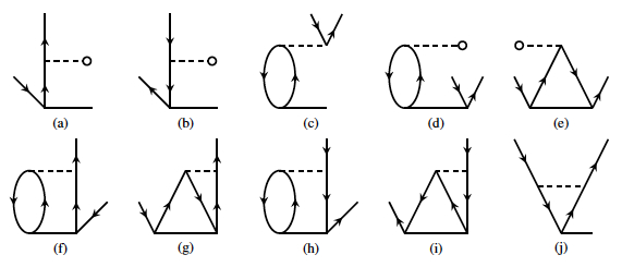
Figure 2: Diagrams which contribute to the linearized RCC for singles ($T_{1}$). Dashed lines represent the residual Coulomb interaction, and the solid lines are the cluster operators.

2.2 Linearized RCC

The dressed Hamiltonian $\bar{H}_{\rm N}$, as given in Eq. (7) have contributions from different orders of $T$, up to quartic. Hence, the Eqs. (9a) and (9b) form a set of non-linear coupled algebraic equations. However, an approximation often used as a starting point of RCC computations is the linearized RCC, where only the linear terms are retained in the computations. In this approximation, the dressed Hamiltonian is

$$\bar{H}_{\rm N}=H_{\rm N}+\bigg{\{}\contraction[0.4ex]{}{H}{{}_{\rm N}}{T}H_{\rm N}T\bigg{\}}.$$ (10)

Using Eq. (10), from Eq. (6) single and double RCC equations are then

$$\langle\Phi^{p}_{a}|H_{\rm N}+\bigg{\{}\contraction[0.4ex]{}{H}{{}_{\rm N}}{T}H_{\rm N}T\bigg{\}}|\Phi_{0}\rangle=0,$$ (11a)

$$\langle\Phi^{pq}_{ab}|H_{\rm N}+\bigg{\{}\contraction[0.4ex]{}{H}{{}_{\rm N}}{T}H_{\rm N}T\bigg{\}}|\Phi_{0}\rangle=0.$$ (11b)

For the CCSD approximation $T=T_{1}+T_{2}$, these equations are then

$$\langle\Phi^{p}_{a}|\bigg{\{}\contraction[0.4ex]{}{H}{{}_{\rm N}}{T}H_{\rm N}T_{1}\bigg{\}}+\bigg{\{}\contraction[0.4ex]{}{H}{{}_{\rm N}}{T}H_{\rm N}T_{2}\bigg{\}}|\Phi_{0}\rangle = -\langle\Phi^{p}_{a}|H_{\rm N}|\Phi_{0}\rangle,$$ (12a)

$$\langle\Phi^{pq}_{ab}|\bigg{\{}\contraction[0.4ex]{}{H}{{}_{\rm N}}{T}H_{\rm N}T_{1}\bigg{\}}+\bigg{\{}\contraction[0.4ex]{}{H}{{}_{\rm N}}{T}H_{\rm N}T_{2}\bigg{\}}|\Phi_{0}\rangle = -\langle\Phi^{pq}_{ab}|H_{\rm N}|\Phi_{0}\rangle.$$ (12b)

The CC diagrams which contribute to $T_{1}$ and $T_{2}$ in the above equations are shown in the Figs. 2 and 3, respectively. Up to this point we have used the notation $\contraction[0.4ex]{}{A}{\ldots}{B}A\ldots B$ to represent contraction between two operators $A$ and $B$. Here after we drop this explicit notation, and the contractions are implied in expressions with products of operators.

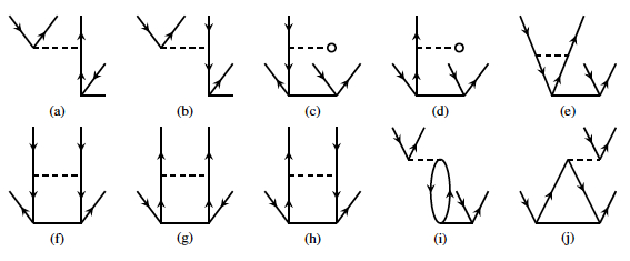
Figure 3: Diagrams which contribute to the linearized RCC for doubles ($T_{2}$). Dashed lines represent the residual Coulomb interaction, and the solid lines are the cluster operators.

The other form of RCC equations is to write in terms of cluster amplitudes, $t^{p}_{a}$ and $t^{pq}_{ab}$. The linearized RCC equation of $T_{1}$ is then

$$\epsilon_{a}^{p}t^{p}_{a}=\sum_{bq}\tilde{v}^{bp}_{qa}t^{q}_{b}+\sum_{bqr}\tilde{v}^{bp}_{qr}t^{qr}_{ba}-\sum_{bcq}v^{bc}_{qa}\tilde{t}^{qp}_{bc},$$ (13)

where $\epsilon_{a}^{p}=\epsilon_{a}-\epsilon_{p}$, $v^{ij}_{kl}$ is the matrix element of electron-electron Coulomb interaction $\langle ij|(1/r_{12})|kl\rangle$, and $\tilde{v}^{ij}_{kl}=v^{ij}_{kl}-v^{ij}_{lk}=v^{ij}_{kl}-v^{ji}_{kl}$ is the antisymmetrized matrix element. Similarly, the compact notation the antisymmetrized CC amplitude is ${\widetilde{t}}^{ij}_{kl}$. Like the $T_{1}$, the linearized RCC equation for $T_{2}$ is

$$\epsilon_{ab}^{pq}t^{pq}_{ab} = v^{pq}_{ab}+\bigg{[}\sum_{r}v^{pq}_{rb}t^{r}_{a}-\sum_{c}v^{cq}_{ab}t^{p}_{c}+\sum_{rc}\Big{(}v^{pc}_{ar}\tilde{t}^{rq}_{cb}-v^{pc}_{rb}t^{rq}_{ac}-v^{cp}_{ar}t^{rq}_{cb}\Big{)}\bigg{]}$$ (16)

$$+\left[\begin{array}[]{c}p\leftrightarrow q\\ a\leftrightarrow b\end{array}\right]+\sum_{rs}v^{pq}_{rs}t^{rs}_{ab}+\sum_{cd}v^{cd}_{ab}t^{pq}_{cd},$$

where $\epsilon_{ab}^{pq}=\epsilon_{a}+\epsilon_{b}-\epsilon_{p}-\epsilon_{q}$ and $\bigl{[}\begin{smallmatrix}p\leftrightarrow q\\ a\leftrightarrow b\end{smallmatrix}\bigr{]}$ represents terms similar to those within parenthesis but with the combined permutations $p\leftrightarrow q$ and $a\leftrightarrow b$. These equations are the algebraic equivalent of the diagrams shown in Figs. 2 and 3, respectively. The evaluations are based on the rules to analyze Goldstone diagrams. It is the preferred scheme as the angular momentum diagram evaluation is easier. At the implementation level, the angular integrals are evaluated so that the equations are in terms of reduced matrix elements of $T$ operators. This minimizes the number of cluster amplitudes and simplify the computations.

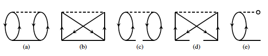
Figure 4: The coupled-cluster diagrams which contribute the correlation energy for closed-shell systems. The dashed lines represent the Coulomb interaction. The solid lines, however, are to represent the CC operators.

2.3 Correlation energy

The correlation energy of a closed-shell system, as defined in Eq. (6a), is the expectation value of $\bar{H}_{N}$ with respect to $|\Phi_{0}\rangle$. That is

$$\Delta E=\langle\Phi_{0}|\bar{H}_{\rm N}|\Phi_{0}\rangle,$$ (17)

and in the CCSD approximation it has contributions from $T_{1}$ and $T_{2}$. The diagrams which contribute to $\Delta E$ are shown in the Fig. 4. The dominant contributions are from the diagrams (a) and (b), which is natural as the $t_{ab}^{pq}$ are larger in value than $t_{a}^{p}$. The other two diagrams, (c) and (d), arise from terms which are second order in $T_{1}$ and have smaller contribution. The last diagram Fig. 4(e), following Koopman’s theorem, is zero when Dirac-Hartree-Fock orbitals are used. Neglecting this diagram, the algebraic expression of $\Delta E$ corresponding to the first four diagrams in Fig. 4 is

$$\Delta E=\tilde{v}_{pq}^{ab}\Big{(}t_{ab}^{pq}+t_{a}^{p}t_{b}^{q}\Big{)}.$$ (18)

This can be computed once the cluster amplitudes are known. Albeit, the correlation equation is written first in eq. 6, but in computations, it is evaluated later.

3 Fock-space CC theory and properties of one-valence systems

The key difference of one-valence atom or ions from the closed-shell ones is the presence of a single electron in the outer most or the valence shell. To account for the correlation effects arising from the valence electron, we use Fock-space coupled-cluster theory and introduce a new set of cluster operators $S$. In the CCSD approximation $S=S_{1}+S_{2}$ and these are defined as

$$S_{1} = \sum_{p}s_{v}^{p}a_{p}^{\dagger}a_{v},$$ (19a)

$$S_{2} = \frac{1}{2!}\sum_{a,p,q}s_{va}^{pq}a_{p}^{\dagger}a_{q}^{\dagger}a_{a}a_{v},$$ (19b)

where, $v$ is the index which identifies the valence electron and $s_{\ldots}^{\ldots}$ are the cluster amplitudes corresponding to the valence sector. In the Fock-space coupled-cluster of one-valence systems, as the name indicates, the starting point of the calculation is the closed-shell coupled-cluster. Based on the Hilbert space of the closed-shell system, we generate the one-valence Hilbert space by adding an electron. These two Hilbert spaces together form the Fock-space for the one-valence system. Thus, the reference state of the one-valence system, starting from the closed-shell system, is $|\Phi_{v}\rangle=a_{v}^{\dagger}|\Phi_{0}\rangle$. Here, recall that $|\Phi_{0}\rangle$ is the Dirac-Hartree-Fock state of the closed-shell system and $a_{v}^{\dagger}$ adds the valence electron. The exact state of the system is

$$|\Psi_{v}\rangle=e^{(T+S)}|\Phi_{v}\rangle=e^{T}(1+S)|\Phi_{v}\rangle.$$ (20)

It is to be noted that the closed-shell part, which involves $T$, are calculated to all orders, or we retain the exponential form of the CCT in the closed-shell sector, but $S$ restricted to linear terms only. This is due to the presence of a single valence electron, and the diagrammatic representations of $S$ are shown in Fig. 5.

Figure 5: Diagrammatic representation of the $S_{1}$ and $S_{2}$ cluster operators. These can be considered as topological transformations of $T_{1}$ and $T_{2}$ cluster operators with one of the core orbital lines rotated downwards as indicated by the arrow and orbital line in gray.

The schematic representation of converting the computation of $T$ to $S$ cluster amplitudes is shown in the figure. It is equivalent to converting one of the core orbitals in the driver programs to valence orbital. Once the cluster amplitudes are obtained, the coupled-cluster wavefunctions can be used for properties computations. For atoms or ions there are, in general, two classes of properties. First, the properties associated with a state which are calculated as expectations, and second, transition properties associated with an initial and final states. The hyperfine structure constants, and electric dipole $E1$ transition properties are described as examples of the former and latter classes, respectively.

3.1 One-valence coupled-cluster equations

The one-valence exact state $|\Psi_{v}\rangle$ satisfies the Schrödinger equation

$$H^{\rm DC}e^{T}(1+S)|\Phi_{v}\rangle=E_{v}|\Phi_{v}\rangle,$$ (21)

where $H^{\rm DC}$ is now the Dirac-Coulomb Hamiltonian in the one-valence sector. Projecting this equation on $e^{T}$, and using the normal form of the Hamiltonian the one-valence cluster amplitudes, in the CCSD approximation, are solutions of the coupled linear equations

$$\langle\Phi_{v}^{p}|\bar{H}_{N}\!+\!\{\contraction[0.5ex]{\bar{}}{H}{{}_{N}}{S}\bar{H}_{N}S\}|\Phi_{v}\rangle = E_{v}^{\rm att}\langle\Phi_{v}^{p}|S_{1}|\Phi_{v}\rangle,$$ (22a)

$$\langle\Phi_{va}^{pq}|\bar{H}_{N}+\{\contraction[0.5ex]{\bar{}}{H}{{}_{N}}{S}\bar{H}_{N}S\}|\Phi_{v}\rangle = E_{v}^{\rm att}\langle\Phi_{va}^{pq}|S_{2}|\Phi_{v}\rangle,$$ (22b)

where, $E_{v}^{\rm att}$ is the attachment energy of the valence shell or the energy released when an electron is attached to the open shell $v$ in the closed-shell ion. The excited determinants $|\Phi^{p}_{v}\rangle$ and $|\Phi^{pq}_{va}\rangle$, like in the case of closed-shell system, are obtained by exciting one and two electron from the reference state $|\Phi_{v}\rangle$. By definition

$$E_{v}^{\rm att}=E_{v}-E_{0},$$ (23)

where $E_{v}=\langle\Phi_{v}|\bar{H}_{N}+\{\contraction[0.5ex]{\bar{}}{H}{{}_{N}}{S}\bar{H}_{N}S\}|\Phi_{v}\rangle$ and $E_{0}=\langle\Phi_{0}|\bar{H}|\Phi_{0}\rangle$ are the exact energies of states $|\Psi_{v}\rangle$ and $|\Psi_{0}\rangle$ respectively. A detailed description of the derivation and interpretations of these equations are given ref [26]. One key difference of Eqs. 22 from the closed-shell case are the terms on the right hand side of the equations, and these are the renormalization terms. In diagrammatic representation, these are the folded diagrams, and have very different topological structure from the $\bar{H}$ or $\contraction[0.5ex]{\bar{}}{H}{{}_{N}}{S}\bar{H}_{N}S$.

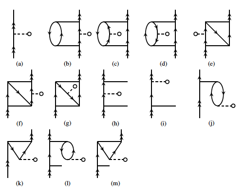
Figure 6: Few of the diagrams with dominant contributions to the hyperfine structure constants in one-valence systems. In the diagrams, the dashed lines marked with open circle represents hyperfine interaction.

3.2 Hyperfine Structure Constants of one-valence systems

For atom or ions in the state $|\Psi_{v}\rangle$ the experimentally measured property $A$ is the expectation

$$\langle A\rangle=\frac{\langle\Psi_{v}|A|\Psi_{v}\rangle}{\langle\Psi_{v}|\Psi_{v}\rangle}.$$ (24)

The property could be associated with either an interaction which is internal or in response to an external perturbation. In the present case, we consider $A$ as the hyperfine interaction $H_{\rm hfs}$ which is internal to the atom or ion. It arises from the coupling of the nuclear electromagnetic moments to the electromagnetic field of the electrons. The total angular momentum of the system is then $F=I+J$, where $I$ and $J$ are the nuclear spin, and total angular momentum of the electrons. The states of the system are represented as $|(IJ)FM_{F}\rangle$, and the form of the hyperfine interaction is [27]

$$H_{\rm hfs}=\sum_{i}\sum_{k,q}(-1)^{q}t^{k}_{q}(\hat{\bf r}_{i})T^{k}_{-q},$$ (25)

where $t^{k}_{q}(\bm{r})$ and $T^{k}_{q}$ represent irreducible tensor operators of rank $k$ in the electron and nuclear spaces, respectively, and index $i$ is summed over all the electrons in the system. Following the parity considerations, only the even and odd values of $k$ are possible for the electric and magnetic interactions, respectively. In general, the parameters which represent the energy shift due to hyperfine interactions are the hyperfine structure constants. For one valence systems, the magnetic dipole hyperfine structure constant is

$$a=\frac{g_{I}\mu_{N}}{\sqrt{j_{v}(j_{v}+1)(2j_{v}+1)}}\langle\Psi_{v}||\sum_{i}t^{1}(\mathbf{r}_{i})||\Psi_{v}\rangle,$$ (26)

where, $j_{v}$ is the total angular momentum of the valence electron, $g_{I}$ is the gyromagnetic ratio and $\mu_{N}$ is the nuclear magneton. In terms of the coupled-cluster wave functions, the reduced matrix element of the hyperfine interaction Hamiltonian is

$$\langle\Psi_{v}\parallel H_{\rm hfs}\parallel\Psi_{v}\rangle=\langle\Phi_{v}\parallel\tilde{H}_{\rm hfs}+2S^{\dagger}\tilde{H}_{\rm hfs}+S^{\dagger}\tilde{H}_{\rm hfs}S\parallel\Phi_{v}\rangle,$$ (27)

where, $\tilde{H}_{\rm hfs}=e{{}^{T}}^{\dagger}H_{\rm hfs}e^{T}$ is the dressed operator. We arrive at the factor of two on the second term on the right hand side as $S^{\dagger}\tilde{H}_{\rm hfs}=\tilde{H}_{\rm hfs}S$. A convenient form of $\tilde{H}_{\rm hfs}$ is

$$\tilde{H}_{\rm hfs}=H_{\rm hfs}e^{T}+\sum_{n=1}^{\infty}\frac{1}{n!}\left(T^{\dagger}\right)^{n}H_{\rm hfs}e^{T},$$ (28)

and the normalization factor is

$$\langle\Psi_{v}|\Psi_{v}\rangle=\langle\Phi_{v}|\left(1+S^{\dagger}\right)e{{}^{T}}^{\dagger}e^{T}\left(1+S\right)|\Phi_{v}\rangle.$$ (29)

In the computations we consider the first few terms in order of the cluster operators from the non-terminating series of $\tilde{H}_{\rm hfs}$, and the operator $e{{}^{T}}^{\dagger}e^{T}$ in the normalization factor. As example, the diagrams corresponding to dominant terms are shown in Fig. 6.

3.3 Electric dipole transition amplitudes for one-valence systems

The electromagnetic transition amplitudes is another class of properties of atoms or ions which involve two states, an initial and final state. Among the various electromagnetic multipole transitions, the electric dipole $E1$ is the most dominant, and occures between two states of opposite parities. In terms of theoretical description, the important quantity related to $E1$ transition between the initial and final states $|\Psi_{i}\rangle$ and $|\Psi_{f}\rangle$, respectively, is

$$D_{if}=\frac{\langle\Psi_{f}\parallel\mathbf{D}\parallel\Psi_{i}\rangle}{\sqrt{\langle\Psi_{f}|\Psi_{f}\rangle\langle\Psi_{i}|\Psi_{i}\rangle}},$$ (30)

where $\mathbf{D}$ is the electric dipole operator. To simplify the expression we can partition the coupled-cluster wave operator as

$$e^{T}(1+S)=\Omega=\Omega^{+}+\Omega^{-}.$$ (31)

Where $\Omega^{+}$ and $\Omega^{-}$ are the components of the wave operator which operates on the even and odd parity reference states. We can, then, write

$$D_{if}=\frac{\langle\Psi_{f}^{0}\parallel{\Omega^{\mp}}^{\dagger}D\Omega^{\pm}\parallel\Psi_{i}^{0}\rangle}{\sqrt{\langle\Psi_{f}|\Psi_{f}\rangle\langle\Psi_{i}|\Psi_{i}\rangle}}.$$ (32)

For the one-valence system if $|\Psi_{v}\rangle$ and $|\Psi_{w}\rangle$ are the initial and final states, respectively, then the reduced matrix element is

$$\langle\Psi_{w}\parallel\mathbf{D}\parallel\Psi_{v}\rangle=\langle\Phi_{v}\parallel\tilde{\mathbf{D}}+S^{\dagger}\tilde{\mathbf{D}}+\tilde{\mathbf{D}}S+S^{\dagger}\tilde{\mathbf{D}}S\parallel\Phi_{v}\rangle.$$ (33)

Albeit the expressions are similar to Eq.(27), there is one important difference. Unlike in the case of hyperfine structure constant $S^{\dagger}\tilde{\mathbf{D}}\neq\tilde{\mathbf{D}}S$ as the $|\Psi_{v}\rangle$ and $|\Psi_{w}\rangle$ are different states. The code in the present work computes the $E$1 reduced matrix elements as the $E$1 transition properties can be obtain from it in combination with the excitation energies. In terms of diagrams, we can obtain the dominant contributions after appropriate modification of the diagrams in Fig. 6. And, the modifications are: changing $H_{\rm hfs}$ to $\mathbf{D}$, and relabelling the final state as the valence state $v$.

4 Computational details

4.1 Radial grid

For numerical evaluation of the two-electron Slater integrals, the radial wave functions are defined in an exponential grid. So that the $i$th radial grid point has the value, in atomic units,

$$r(i)=r_{0}\left[e^{(i-1)h}-1\right],$$ (34)

where, for the present work, we use $r_{0}=2.0\times 10^{-6}$ and $h=0.05$. This choice of radial grid representation samples the nuclear Coulomb potential very well: smaller separation in the $r\ll 1$ and larger separation at $r\gg 1$, where the potential is strong and weak, respectively. This choice is similar to the grid used in GRASP2K [28]. In the present implementation of the code, the details of the grid are read from the orbital basis file. The obvious advantage of this implementation is the consistent choice of grid parameters across codes as we generate the basis set using another code.

4.2 Orbital basis set

The single particle state $\psi_{n\kappa m}$ with principal quantum number $n$, relativistic total quantum number $\kappa$, and magnetic quantum number $m$ is defined as the four-component spin-orbital

$$\psi_{n\kappa m}(\bm{r})=\frac{1}{r}\left(\begin{array}[]{r}P_{n\kappa}(r)\chi_{\kappa m}(\mathbf{r}/r)\\ iQ_{n\kappa}(r)\chi_{-\kappa m}(\mathbf{r}/r)\end{array}\right),$$ (35)

where $P_{n\kappa}(r)$ and $Q_{n\kappa}(r)$ are the large and small component of the radial wave functions, respectively, and $\chi_{\kappa m}(\mathbf{r}/r)$ are the spinor spherical harmonics. In the example calculations, the radial functions are even tempered Gaussian type orbitals (GTOs) [29] on a grid [30]. The large component $P_{n\kappa}(r)$ are then linear combination of the Gaussian type functions

$$g_{\kappa p}^{L}(r)={\rm N}^{L}_{\kappa p}r^{n_{\kappa}}e^{-\alpha_{p}r^{2}},$$ (36)

where, ${\rm N}^{L}_{\kappa p}$ is the normalization constant, and $\alpha_{p}$ is the exponent. The exponents are defined in terms of two parameters and forms a geometric series $\alpha_{p}=\alpha_{0}\beta^{p-1}$, where $\alpha_{0}$ and $\beta$ are two constants. The choice of these constants are optimized to matched the self consistent field and single particle energies obtained from GRASP2K [28]. The large component can then be written as

$$P_{n\kappa m}(r)=\sum_{p}^{n_{\kappa}}C^{L}_{\kappa p}g_{\kappa p}^{L}(r),$$ (37)

where $C^{L}_{\kappa p}$ is the coefficient of linear combination and $n_{\kappa}$ is the number of Gaussian type functions considered for the symmetry. Using the GTOs, the Slater integrals or the two-electron Coulomb interaction matrix elements are computed using the subroutines from GRASP2K [28].

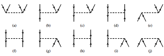
Figure 7: Diagrams of the ten topologically unique representations of the Slater integrals. All the diagrams contribute to the $T_{2}$ equation, but the first three diagrams (a-c) do not contribute to $T_{1}$.

5 Details of implementation

5.1 Loop structures

To aid the conversion from closed-shell to open shell calculations, the implementation has a two-tier structure. These translate to heirarchies of loop structures in terms of the orbitals. For single excitation cluster operator $t_{a}^{p}$ , the first tier consists of loops corresponding to the free orbital lines $p$ and $a$. Similarly, for double excitation cluster operators $t_{ab}^{pq}$, the $p$, $q$, $a$ and $b$ form the outer loops. We refer to this outer loop structure as cluster driven.

To describe the second tier of loops, we classify the Slater integrals into different categories. In total there are ten topologically unique diagrammatic representations, and these are shown in Fig. 7(a-j). The diagrams in the figure correspond to, following the notations introduced earlier, $v_{ab}^{pq}$, $v_{ra}^{qp}$, $v_{ba}^{cp}$, $v_{ar}^{cp}$, $v_{ra}^{cp}$, $v_{ab}^{cd}$, $v_{ar}^{cd}$, $v_{rs}^{pq}$, $v_{rs}^{pc}$ and $v_{rs}^{cd}$. While evaluating the terms in the cluster equations, the lines below the interaction line (dashed lines) or the orbitals with the indexes $r$, $s$, $c$ and $d$, contract with the cluster operators. We refer to these lines as the internal indices. The others, namely $p$, $q$, $a$ and $b$ are the external indices. An advantage of these classifications and definitions is, one immediately notices that the Slater integrals with more than two external lines do not contribute to the $T_{1}$ equation. In particular, the Slater integrals which do not contribute to $T_{1}$ are $v_{ab}^{pq}$, $v_{ra}^{qp}$ and $v_{bc}^{cp}$ but, all the Slater integrals contribute to the $T_{2}$ equation.

In the second tier, the loops are grouped depending on the Slater integrals. For example, in the linearized RCC, $H_{\rm N}T_{1}^{(0)}$ contributes through two channels of contractions $v_{rb}^{pq}t_{a}^{r}$ and $v_{ab}^{cq}t_{c}^{p}$. Here, as mentioned earlier, the product of the operators $H_{\rm N}T_{1}^{(0)}$ imply all possible contractions. The two terms arise from two different types of Slater integrals. A more complicated example is the contribution from $v_{rs}^{pc}$, it does not contribute to the $T_{2}$ equations at the linear level but contributes through the nonlinear terms $H_{\rm N}T_{2}^{(0)}T_{1}^{(0)}$ and $H_{\rm N}T_{1}^{(0)}T_{1}^{(0)}T_{1}^{(0)}$. This grouping of diagrams based on the Slater integrals is equivalent of integral driven in a limited sense. Collectively, we refer to the two-tiered loop structure as the cluster-integral driven.

5.2 Memory parallel integral storage

The RCC equations are nonlinear algebraic equations and are solved iteratively using standard numerical methods. In the present work, we use Jacobi iteration and convergence is accelerated with DIIS [31]. For improved performance, we store the Slater integrals in memory (RAM). The storage of the four particle integrals $v_{rs}^{pq}$, however, require very large memory. For example, in the present calculations the number of the particle states $N_{v}>100$ and the order of memory required to store all the $v_{rs}^{pq}$ in double precision scales as $O[10N_{v}^{4}]=O[10^{9}]$ bytes. Where, the factor of ten accounts for the eight bytes to represent a real number in double precision, and the number of multipoles in each integral. This is a conservative estimate, the actual requirement may exceed this by a factor between five and ten. Although the memory required is manageable with current technologies, it is still a large requirement.

With a straight forward and trivial parallelization, it is possible to divide and parallelize the compute intensive part of the calculations. In a distributed memory environment or cluster computers, one of the more prevalent architecture within the high performance computing community, the storage of $v_{rs}^{pq}$ has a large memory foot print. More over, the same set of integrals are stored across all nodes and leads to replication of data. This is rather expensive and could be a severe bottle neck to exploit parallel computing for calculations with large basis sizes. In the present work, we present an implementation where there are no memory replications while storing $v_{rs}^{pq}$. In other words, the storage of the $v_{rs}^{pq}$ is distributed across the nodes or done in parallel. We refer to this scheme as the memory parallel implementation.

The memory parallel storage of the $v_{rs}^{pq}$ takes advantage of the cluster-integral driven structure of the code. The implementation exploits one feature of this structure: the orbitals lines of the external loops are not contracted. So, we can parallelize any of the external loops, as it is common to all the cluster diagrams. However, for improved performance we choose the particle line for parallelization. This ensures nearly equal workload for all the nodes as the number of particle states is usually an order magnitude larger than the number of core states. For the present discussion, let us assume that the $p$ loop is parallelzed across $N_{n}$ processors of a distributed memory system. In general, for the type of calculations we are interested $N_{n}<N_{v}$, and each of the processors, then, store $O[(10N_{v}^{4})/N_{n}]=O[10^{9}/N_{n}]$ of the four particle Slater integrals $v_{rs}^{pq}$. For example, if $5N_{n}\approx N_{v}$, a condition met in most of our routine computations, we get the memory required per processor as $\approx 2\times 10^{8}$. This is less than one gigabyte and hence, we can increase the basis set size without memory constraints.

Figure 8: The example diagrams which contribute to the RCC term $H_{\rm N}T_{2}T_{2}$ for doubles. Diagram (b) is the exchange at the vertex of $T_{2}$.

5.3 Intermediate storage

The group of CC diagrams for $T_{2}$ which arise from the Slater integral $v^{pq}_{ab}$ involves four contractions, total of eight orbital lines and summation over three multipoles. The evaluation of these diagrams requires the maximum number of loops, and hence the CPU time. Consider, for example, one of the nonlinear terms $\langle\Phi^{pq}_{ab}|H_{\rm N}T_{2}T_{2}|\Phi_{0}\rangle$, which is quadratic in $T_{2}$. There are 22 diagrams which contribute to this term and two are shown in the Fig 8. The second diagram in this figure arise due to exchange at one of the $T_{2}$.

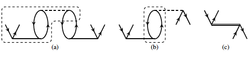
Figure 9: The representation of (a) a common part of the RCC diagram, (b) the IMS diagram and (c) the effective operator diagram.

In both the diagrams, the number of hole and particle orbital lines are four each, and three multipole lines. The total number of operations (NOP) required to evaluate the diagram in Fig. 8(a) is ${N_{h}}^{4}{N_{p}}^{4}{N_{k}}^{3}$. Here, $N_{h}$, $N_{p}$ and $N_{k}$ represent the number of holes, particles and multipoles used in the computations, respectively. Considering the case of Na⁺ as an example, $N_{h}$ is 4, for a reasonable basis size $N_{p}$ can be 100, and since we include orbitals up to $h$-symmetry we may take $N_{k}=11$. The total NOP is then $\approx 3.4\times 10^{13}$. An important point to note is, this number corresponds to Na⁺ which is a lighter ionic system. In the case of high-$Z$ atoms, where the number of holes states are large, the total NOP may increase significantly.

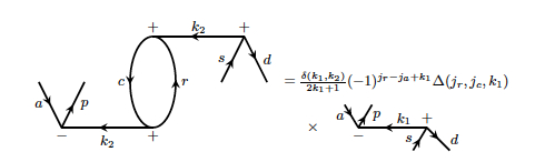
Figure 10: The angular reduction of the IMS diagram. The free part on the right-hand side indicates the form of the effective operator.

One way to reduce the computational time is through the use of IMS scheme. In this approach, a common part of the CC diagrams is identified and calculated separately. This is then stored as an effective operator. This effective operator latter contracts with the CC operator to provide the contribution equivalent to the actual CC diagrams. The common part is referred to as the intermediate storage (IMS) diagram. As shown in the Fig. 9(a), the portion within the dashed line is common to both diagrams in Fig. 8, and is therefore an IMS diagram. The common portion is shown as a separate diagram in Fig. 9(b). The next step is to evaluate this IMS diagram and store in the form of an effective operator. The angular reduction of the IMS diagram is shown in the Fig. 10, where the removal of the closed loop has reduced it to angular factors and a diagram of free lines. It is to be observed that the diagram with free lines is topologically similar to the effective operator shown in Fig. 9(c). The final step to evaluate the CC diagram is to contract the effective operator with the $T_{2}$ operator. The diagrams which arise from the contractions are shown in the Fig. 11. These are equivalent to the diagrams in the Fig. 8.

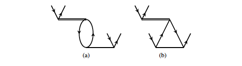
Figure 11: The diagrams arise when effective operator is contracted with $T_{2}$. (a) Equivalent to Fig. 8(a). (b) Equivalent to the exchange diagram Fig. 8(b).

After the implementation of computations with the IMS diagrams, the total NOP required to compute the diagram in Fig. 8(a) is the sum of NOP to compute the diagrams in Fig. 9(b) and Fig. 11(a). Using the analysis discussed earlier, this is $2N^{3}_{h}N^{3}_{p}N^{2}_{k}$, which smaller by a factor of $1/2N_{h}N_{p}N_{k}$. For the example of Na⁺, the NOP required is $\approx 1.5\times 10^{10}$. The advantage of using IMS becomes more evident when we consider both diagrams in the Fig. 8. The total NOP require is $3N^{3}_{h}N^{3}_{p}N^{2}_{k}$, which for Na⁺ example is $\approx 2.3\times 10^{10}$. However, without the use of IMS scheme it is $\approx 6.8\times 10^{13}$.

6 Description of RCCPAC

6.1 Input data files

The package requires two input data files: the orbital basis file; and the data file which provides information about the type of orbitals.

Orbital file–The default name of the orbital file is wfn.dat and it is in binary format. The contents of the file are accessed with a call to the subroutine in readorb.f. It has the following data:

First two records
The first two records pertains to the spatial grid on which the orbitals are defined. The first record has the grid parameters h and n. The second record contains the arrays r, rp and rpor. For the exponential grid used, the first is the grid point, second is the scaling factor required in the integration and last is the rp/r. These two records are accessed by the subroutine in readorb.f as follows:

  read(WFNIN)h, n
  read(WFNIN)(r(i), i = 1, n), (rp(i), i = 1, n), (rpor(i), i = 1, n)

Remaining records
In the remaining part of the file, there are two records for each orbital. The first is the orbital energy, and the second stores the arrays of the large and small components of the orbitals. The records are grouped into orbitals of the same symmetries with increasing $j$. For example, the core orbitals are accessed in readorb.f as follows:

   read(WFNIN)eorb(indx1)
   read(WFNIN)(pf(ii,indx1),ii=1,n),(qf(ii,indx1),ii=1,n)

and then, the virtual orbitals of the same symmetry are read next. This is repeated till orbitals of all the symmetries are read.

Basis and option file–The default name of the data file which has the information about the orbital basis is rccpac.in. It is an ASCII file and consists of the following lines: atomic weight, number of symmetries, and total number of orbitals, valence and core of each symmetry. For the closed-shell case, the number of valence orbitals is zero and the information is not really required. We, however, introduce it, so that the code may be upgraded for one-valence systems with minimal modifications. As an example, consider the case of atomic Na, the contents of rccpac.in for computation with an orbital set consisting of nine symmetries is as given below:

22.99
2
9
19   0    2
15   0    1
15   0    1
13   0    0
13   0    0
11   0    0
11   0    0
9    0    0
9    0    0

The entry ( 22.99) in the first line is the atomic weight of ²³Na and the next line is the option of the computation. The various possible values of option are: 2 for the closed-shell cluster amplitude computations; 4 for the one-valence cluster amplitude computations; and 8 for the one-valence properties computations. To combine the computations, the option of the individual cases must be summed. For example, the value of option to compute the cluster amplitudes of the closed-shell and one-valence sector is 6. The sum of 2 and 4, the values of option to do the computations of closed-shell and one-valence cluster amplitudes. The next line gives the number of symmetries (9) considered in the present computation. The symmetries are namely, $s_{1/2}$, $p_{1/2}$, $p_{3/2}$, $d_{3/2}$, $d_{5/2}$, $f_{5/2}$, $f_{7/2}$, $g_{7/2}$ and $g_{9/2}$. The third line provides information about the $s_{1/2}$ orbitals in the basis. In this line, the entry 19 is the total number of orbitals in $s_{1/2}$ symmetry, and the other two entries 0 and 2 are the number of valence and core orbitals in the $s_{1/2}$ symmetry. Similarly, the remaining lines provide information about the orbitals in the remaining symmetries and in the sequence listed earlier.

Next, as an example, we provide the contents of the input file of one-valence computations for ¹³³Cs. In this case the value of option is set as 14, which is the sum of 2, 4, and 8. These are the options corresponding to the computations of close-shell and one-valence cluster amplitude, and one-valence properties. The contents of the input file is as given below:

132.91
14
9
17  1  5
13  1  4
13  1  4
13  1  2
13  1  2
11  0  0
11  0  0
11  0  0
11  0  0
13  0  0
13  0  0
13  0  0
13  0  0

The key difference of the input file compared to the previous example is the inclusion of data about the valence shells, the non-zero values in the second column on information about the basis functions. The non-zero values in the present case represent the valence orbitals of $6s$, $6p_{1/2}$, $6p_{3/2}$, $5d_{3/2}$, and $5d_{5/2}$, respectively.

6.2 Constant parameters

The dimension of the arrays and various other parameters required in different sections of the package are defined as parameters in the module param. The module is part of the main subroutine file rccpac.f and in the present version of the package the module is defined as follows:

      module param
        integer, parameter :: NHO = 27,  NPO = 170, MXL = 25, MXV = 20,
     &                        MDIM = 6000000, MN  = 950, MNSYM = 13,
     &                        MNS = 13, MXVR  = (MXV+1)/2, MNBAS = NHO+NPO,
     &                        MNOCC = NHO, MNEXC =  NPO,
        integer, parameter :: STDIN = 5, WFNIN = 7,NTFILE = 16,
     &                        STDOUT = 8,MASTER = 0, STDIMS = 9, NITMAX = 50,
     &                        NPMAX = 128, PUNCH = 17

        real (8), parameter:: SMALL = 1.2d-8
      end module param

In the module, the first set of parameters define the maximum number of a data set and these are as follows:
      NHO: core orbitals, NPO: virtual orbitals, MXL: multipoles of the cluster amplitudes, MXV: multipoles of the two-electron interaction, MDIM: cluster amplitudes, MN: grid points used to define the orbitals, MNSYM: symmetries of orbitals, MNS: symmetries of orbitals,
The second group of parameters are related to I/O and iterations used in the computations. These are:
      STDIN: Unit number of the input file, WFNIN: Unit number of the orbital data file, NTFILE: STDOUT: Unit number of default output, MASTER: identity of the master in the MPI execution of the package, STDIMS: NITMAX: maximum number of iteration in the Jacobi method to solve the cluster equations, NPMAX:
The last element in the module, SMALL, is the parameter which is used to define the convergence criterion.

6.3 Output data

On the successful completion the package generates the coupled-cluster amplitudes and these are stored in the binary data file ccamp_0v.dat. The information related to computation are given in the output file rccpac.out. The file has data about the orbital basis, number of two-electron integrals, number of IMS diagrams in each group, convergence parameter, and details of the DIIS computation.

    *****************************************************************
    *****************************************************************
                RELATIVISTIC COUPLED-CLUSTER PROGRAM
                               for
                       ATOMIC CALCULATIONS
                             (RCCPAC)
        Relativistic coupled-cluster theory with single and double
        excitation approximation is implemented in this code.
        The cluster equations are solved using Jacobi iteration
        with Direct Inversion in the Iterative Subspace (DIIS) to
        accelerate the convergence.

        Written by

        Brajesh K. Mani              Physical Research Laboratory
        Siddhartha Chattopadhyay     Theoretical Physics Division
        Dilip Angom                  Navarangpura, Ahmedabad--09
                                     Gujarat, INDIA

    *****************************************************************
    *****************************************************************

DATE :
 Tue Jun 21 13:27:27 2016
 The number of orbitals in the core (ncore) =   4
                             valence (nval) =   0
                            occupied (nocc) =   4
                           virtual (nexcit) = 111
                             total (nbasis) = 115

-------------------------------------------------------------------------------
               ++Completed RCC (T0) skip calculations (symm.f)++
-------------------------------------------------------------------------------
 Number of single excited cluster amplitudes:         62
           double excited cluster amplitudes:      27364

-------------------------------------------------------------------------------
               ++Completed reading radial wave functions++
-------------------------------------------------------------------------------
  Core orbitals
  -------------
  Seq no.             Orbital Energy

     1                  -40.82654629
     2                   -3.08240070
     3                   -1.80141924
     4                   -1.79401059

  ----------------
  Virtual orbitals
  ----------------
  Seq no.             Orbital Energy

     5                   -0.18203250
     6                   -0.07016031
     7                   -0.03703966
     8                   -0.01737279
     9                    0.05584768
    10                    0.31893785
   ***                  ************
   113                   14.53407907
   114                   38.87397690
   115                  105.24442393
-------------------------------------------------------------------------------
        ++Entering coul_tab to tabulate two-electron Coulomb integrals++
-------------------------------------------------------------------------------

 The maximum number of <ph|v|hp> ( nskip_phhp) is:        54204
                       <hh|v|hh> ( nskip_hhhh) is:          109
                       <ph|v|ph> ( nskip_phph) is:        50252
                       <pp|v|pp> ( nskip_pppp) is:     78252104
                       <hh|v|pp> ( nskip_hhpp) is:        54204
                       <pp|v|hp> ( nskip_pphp) is:      1945909
                       <hp|v|pp> ( nskip_hppp) is:      1945909
                       <ph|v|hh> ( nskip_phhh) is:         1785
                       <hh|v|ph> ( nskip_hhph) is:         1785

 init_close1, nsing           0          62
-------------------------------------------------------------------------------
             ++Linearised unperturbed closed-shell (ldrivert0_0v)++
-------------------------------------------------------------------------------
 Convergence parameter is   0.120000D-07

 Iteration   1
       conv and convd are =   0.615626D-01      0.138845D+01
       eps  and epsd  are =   0.992945D-03      0.507402D-04

 Iteration   2
       conv and convd are =   0.415324D-02      0.270568D+00
       eps  and epsd  are =   0.669878D-04      0.988775D-05

       DIIS matrix elements
           1    1  0.139833D-02
           1    2 -0.139262D-04
           2    2  0.393844D-04
       DIIS solution
             0.363755D-01      0.963625D+00      0.374452D-04

 *********   ************      ***********      *************

 Iteration   7
       conv and convd are =   0.211860D-04      0.157455D-03
       eps  and epsd  are =   0.341710D-06      0.575409D-08

 Converged in **  7** iterations


 Maximum number of nskip_ims4p is:    156081572
                   nskip_ims4h is:          406
                 nskip_ims2p2h is:       212722
                 nskip_imsphhh is:         7293
                 nskip_imspphp is:      7727007

-------------------------------------------------------------------------------
             ++Nonlinear unperturbed closed-shell (nldrivert0_0v)++
-------------------------------------------------------------------------------
 Convergence parameter is   0.120000D-07

 Iteration   1
       conv and convd are =   0.204806D-02      0.125925D+00
       eps  and epsd  are =   0.330333D-04      0.460186D-05

 Iteration   2
       conv and convd are =   0.628172D-03      0.219799D-01
       eps  and epsd  are =   0.101318D-04      0.803242D-06

       DIIS matrix elements
           1    1  0.149170D-04
           1    2  0.146607D-05
           2    2  0.390725D-06
       DIIS solution
            -0.868926D-01      0.108689D+01      0.297286D-06

*********   ************      ***********      *************

 Iteration   5
       conv and convd are =   0.165985D-04      0.301626D-03
       eps  and epsd  are =   0.267719D-06      0.110227D-07

       DIIS matrix elements
           1    1  0.112876D-08
           1    2  0.302626D-09
           2    2  0.102218D-09
       DIIS solution
            -0.320281D+00      0.132028D+01      0.380308D-10
 Converged in **  5** iterations


-------------------------------------------------------------------------------
                        ++Compute correlation energy++
-------------------------------------------------------------------------------

 Correlation energy ( in atomic units):
       Contribution from direct   diagrams:   -0.5781920
       Contribution from exchange diagrams:    0.2088729
                                     Total:   -0.3693191

DATE :
 Tue Jun 21 13:41:38 2016

In the printout of the output file rccpac.out, the rows with *** indicate additional lines of data, but not included in the above for compactness. Albeit, we have given the correlation energy as an example of the property computed using the CCSD wavefunction, any other properties of a closed-shell atom or ion may be computed using the cluster amplitudes in the output file ccamp_0v.dat.

For the case of one-valence systems, the contents of the output file of the properties computations of ¹³³Cs is given below as an example. The computation of the E1 reduced matrix elements is given as an example of the one-valence properties. The hyperfine structure constants can also be computed in the same way.

    *****************************************************************
    *****************************************************************
                RELATIVISTIC COUPLED-CLUSTER PROGRAM
                               for
                       ATOMIC CALCULATIONS
                             (RCCPAC)


        Relativistic coupled-cluster theory with single and double
        excitation approximation is implemented in this code.
        The cluster equations are solved using Jacobi iteration
        with Direct Inversion in the Iterative Subspace (DIIS) to
        accelerate the convergence.


        Written by

        Brajesh K. Mani              Physical Research Laboratory
        Siddhartha Chattopadhyay     Theoretical Physics Division
        Dilip Angom                  Navarangpura, Ahmedabad--09
                                     Gujarat, INDIA

    *****************************************************************
    *****************************************************************



DATE :
 Mon Oct 17 12:24:45 2016
 The number of orbitals in the core (ncore) =  17
                             valence (nval) =   5
                            occupied (nocc) =  22
                           virtual (nexcit) =  96
                             total (nbasis) = 113

-------------------------------------------------------------------------------
               ++Completed RCC (T0) skip calculations (symm.f)++
-------------------------------------------------------------------------------
 Number of single excited cluster amplitudes:        228
           double excited cluster amplitudes:     868773


-------------------------------------------------------------------------------
               ++Completed reading radial wave functions++
-------------------------------------------------------------------------------
  Core orbitals
  -------------
  Seq no.             Orbital Energy

     1                -1330.11726503
     2                 -212.56429987
     3                  -45.96972982
     4                   -9.51278742
     5                   -1.48980491
     6                 -199.42944490
     7                  -40.44831432
     8                   -7.44627286
     9                   -0.90789762
    10                 -186.43662752
    11                  -37.89433600
    12                   -6.92099140
    13                   -0.84033940
    14                  -28.30956867
    15                   -3.48562841
    16                  -27.77522550
    17                   -3.39691055

  ----------------
  Valence orbitals
  ----------------
  Seq no.             Orbital Energy

    18                   -0.12736841
    19                   -0.08561350
    20                   -0.08378191
    21                   -0.06440672
    22                   -0.06451711

  ----------------
  Virtual orbitals
  ----------------
  Seq no.             Orbital Energy

    23                   -0.05283804
    24                    0.02231458
    25                    0.24902056
    26                    0.92053859
    27                    2.87599696
   ***                  ************
   111                   70.38575916
   112                  207.56873070
   113                  611.39136250
-------------------------------------------------------------------------------
        ++Entering coul_tab to tabulate two-electron Coulomb integrals++
-------------------------------------------------------------------------------


 The maximum number of <ph|v|hp> ( nskip_phhp) is:      1734444
                       <hh|v|hh> ( nskip_hhhh) is:        97234
                       <ph|v|ph> ( nskip_phph) is:      1697124
                       <pp|v|pp> ( nskip_pppp) is:     53166820
                       <hh|v|pp> ( nskip_hhpp) is:      1734444
                       <pp|v|hp> ( nskip_pphp) is:      9290442
                       <hp|v|pp> ( nskip_hppp) is:      9290442
                       <ph|v|hh> ( nskip_phhh) is:       353553
                       <hh|v|ph> ( nskip_hhph) is:       353553

 init_close1, nsing           0         228
********************************************************************************
                     Output from the closed-shell part
********************************************************************************
-------------------------------------------------------------------------------
             ++Linearised unperturbed one-valence (ldrivert0_1v)++
-------------------------------------------------------------------------------
 Convergence parameter is   0.120000D-07
       Attachement energies
       Valence Orb       Corr Energy       Orb Energy       Attach Energy
            18          -0.166919D-01     -0.127368D+00    -0.144060D+00
            19          -0.655392D-02     -0.856135D-01    -0.921674D-01
            20          -0.592481D-02     -0.837819D-01    -0.897067D-01
            21          -0.100909D-01     -0.644067D-01    -0.744976D-01
            22          -0.972703D-02     -0.645171D-01    -0.742441D-01

 Iteration   1
       conv and convd are =   0.229040D+01      0.630055D+02
       eps  and epsd  are =   0.100456D-01      0.725224D-04

       Attachement energies
       Valence Orb       Corr Energy       Orb Energy       Attach Energy
            18          -0.134525D-01     -0.127368D+00    -0.140821D+00
            19          -0.544351D-02     -0.856135D-01    -0.910570D-01
            20          -0.492562D-02     -0.837819D-01    -0.887075D-01
            21          -0.763087D-02     -0.644067D-01    -0.720376D-01
            22          -0.738749D-02     -0.645171D-01    -0.719046D-01


 *********   ************      ***********      *************

 Iteration  10
       conv and convd are =   0.580033D-03      0.117220D-01
       eps  and epsd  are =   0.254401D-05      0.134926D-07

       Attachement energies
       Valence Orb       Corr Energy       Orb Energy       Attach Energy
            18          -0.169498D-01     -0.127368D+00    -0.144318D+00
            19          -0.692914D-02     -0.856135D-01    -0.925426D-01
            20          -0.620691D-02     -0.837819D-01    -0.899888D-01
            21          -0.136117D-01     -0.644067D-01    -0.780185D-01
            22          -0.128607D-01     -0.645171D-01    -0.773778D-01

 Iteration  11
       conv and convd are =   0.333555D-03      0.447109D-02
       eps  and epsd  are =   0.146296D-05      0.514645D-08

 Converged in ** 11** iterations


-------------------------------------------------------------------------------
             ++Nonlinear unperturbed one-valence (nldrivert0_1v)++
-------------------------------------------------------------------------------
 Convergence parameter is   0.120000D-07
       Attachement energies
       Valence Orb       Corr Energy       Orb Energy       Attach Energy
            18          -0.169508D-01     -0.127368D+00    -0.144319D+00
            19          -0.692949D-02     -0.856135D-01    -0.925430D-01
            20          -0.620722D-02     -0.837819D-01    -0.899891D-01
            21          -0.136117D-01     -0.644067D-01    -0.780184D-01
            22          -0.128606D-01     -0.645171D-01    -0.773777D-01

 Iteration   1
       conv and convd are =   0.410651D+00      0.359759D+01
       eps  and epsd  are =   0.180110D-02      0.414100D-05

       Attachement energies
       Valence Orb       Corr Energy       Orb Energy       Attach Energy
            18          -0.164705D-01     -0.127368D+00    -0.143839D+00
            19          -0.666249D-02     -0.856135D-01    -0.922760D-01
            20          -0.588440D-02     -0.837819D-01    -0.896663D-01
            21          -0.131382D-01     -0.644067D-01    -0.775449D-01
            22          -0.124401D-01     -0.645171D-01    -0.769572D-01

 *********   ************      ***********      *************

 Iteration   9
       conv and convd are =   0.492117D-03      0.474424D-02
       eps  and epsd  are =   0.215841D-05      0.546085D-08

       DIIS matrix elements
           1    1  0.585631D-06
           1    2  0.166541D-06
           1    3  0.146858D-06
           1    4  0.565027D-07
           2    2  0.259704D-06
           2    3  0.480579D-07
           2    4  0.887415D-07
           3    3  0.398448D-07
           3    4  0.155797D-07
           4    4  0.316634D-07
       DIIS solution
            -0.131591D+00     -0.321214D+00      0.549912D+00
             0.902893D+00      0.121586D-08
 Converged in **  9** iterations


       Attachement energies
       Valence Orb       Corr Energy       Orb Energy       Attach Energy
            18          -0.163371D-01     -0.127368D+00    -0.143705D+00
            19          -0.660373D-02     -0.856135D-01    -0.922172D-01
            20          -0.583622D-02     -0.837819D-01    -0.896181D-01
            21          -0.119459D-01     -0.644067D-01    -0.763527D-01
            22          -0.113554D-01     -0.645171D-01    -0.758725D-01
-------------------------------------------------------------------------------
               ++One-valence properties computations (prop_1v)++
-------------------------------------------------------------------------------
 Normalization

    State     Normalization factor

      18         0.993542
      19         0.996916
      20         0.997362
      21         0.993279
      22         0.993639

  Final state      Intial state                      E1 amplitude
       1                  2       DF value             -5.228273
                                  Total value          -4.494237

       1                  3       DF value             -7.360728
                                  Total value          -6.350515

       2                  1       DF value             -5.228273
                                  Total value          -4.500968

       2                  4       DF value              8.874962
                                  Total value           7.313672

       2                  5       DF value              0.000000
                                  Total value           0.000000

       3                  1       DF value              7.360728
                                  Total value           6.368736

       3                  4       DF value              4.015906
                                  Total value           3.293150

       3                  5       DF value             12.051371
                                  Total value           9.995387

       4                  2       DF value             -8.874962
                                  Total value          -7.327270

       4                  3       DF value              4.015906
                                  Total value           3.294046

       5                  2       DF value              0.000000
                                  Total value           0.000000

       5                  3       DF value            -12.051371
                                  Total value          -9.982575


DATE :
 Mon Oct 17 19:10:23 2016

In the output file shown above, the states identified as 1, 2, 3, 4, and 5 correspond to the $6s(^{2}S_{1/2})$, $6p(^{2}P_{1/2})$, $6p(^{2}P_{3/2})$, $5d(^{2}D_{3/2})$ and $5d(^{2}D_{5/2})$ states of Cs. The hyperfine structure constants can also be computed in the same way by choosing the hyperfine structure constant subroutine in the main driver subroutine rccpac.f where the properties driver subroutine prop_1v.f is called. In the case of hyperfine structure constants, the output from the code gives the matrix elements of the hyperfine interaction Hamiltonian in the electronic sector. So, to obtain the hyperfine structure constants in the units of MHz, the results obtain from the code should be multiplied by the gyromagnetic ratio of the atom or ion, and factor of 13074.69. For compactness we have not shown the contents of the output file for the hyperfine structure constant computations.

References

References

- Coester [1958] F. Coester, Nucl. Phys. 7 (1958) 421 – 424.
- Coester and Kümmel [1960] F. Coester, H. Kümmel, Nucl. Phys. 17 (1960) 477 – 485.
- Čížek [1966] J. Čížek, J. Chem. Phys. 45 (1966) 4256.
- Čížek [1969] J. Čížek, Adv. Chem. Phys. 14 (1969) 35–89.
- Hagen et al. [2014] G. Hagen, T. Papenbrock, M. Hjorth-Jensen, D. J. Dean, Rep. Prog. Phys. 77 (2014) 096302.
- Gopakumar et al. [2001] G. Gopakumar, H. Merlitz, S. Majumder, R. K. Chaudhuri, B. P. Das, U. S. Mahapatra, D. Mukherjee, Phys. Rev. A 64 (2001) 032502.
- Pal et al. [2007] R. Pal, M. S. Safronova, W. R. Johnson, A. Derevianko, S. G. Porsev, Phys. Rev. A 75 (2007) 042515.
- Mani et al. [2009] B. K. Mani, K. V. P. Latha, D. Angom, Phys. Rev. A 80 (2009) 062505.
- Isaev et al. [2004] T. A. Isaev, A. N. Petrov, N. S. Mosyagin, A. V. Titov, E. Eliav, U. Kaldor, Phys. Rev. A 69 (2004) 030501.
- Li et al. [2014] P. H. Y. Li, R. F. Bishop, C. E. Campbell, Phys. Rev. B 89 (2014) 220408.
- Čárskỳ et al. [2010] P. Čárskỳ, J. Paldus, J. Pittner, Recent Progress in Coupled Cluster Methods: Theory and Applications, Challenges and Advances in Computational Chemistry and Physics, Springer, 2010.
- Bartlett and Musiał [2007] R. J. Bartlett, M. Musiał, Rev. Mod. Phys. 79 (2007) 291–352.
- Purvis and Bartlett [1982] G. D. Purvis, R. J. Bartlett, J. Chem. Phys. 76 (1982) 1910–1918.
- Nataraj et al. [2008] H. S. Nataraj, B. K. Sahoo, B. P. Das, D. Mukherjee, Phys. Rev. Lett. 101 (2008) 033002.
- Latha et al. [2009] K. V. P. Latha, D. Angom, B. P. Das, D. Mukherjee, Phys. Rev. Lett. 103 (2009) 083001.
- Wansbeek et al. [2008] L. W. Wansbeek, B. K. Sahoo, R. G. E. Timmermans, B. P. Das, D. Mukherjee, Phys. Rev. A 78 (2008) 012515.
- Sahoo et al. [2009] B. K. Sahoo, B. P. Das, D. Mukherjee, Phys. Rev. A 79 (2009) 052511.
- Chattopadhyay et al. [2012a] S. Chattopadhyay, B. K. Mani, D. Angom, Phys. Rev. A 86 (2012a) 022522.
- Chattopadhyay et al. [2012b] S. Chattopadhyay, B. K. Mani, D. Angom, Phys. Rev. A 86 (2012b) 062508.
- Chattopadhyay et al. [2013a] S. Chattopadhyay, B. K. Mani, D. Angom, Phys. Rev. A 87 (2013a) 042520.
- Chattopadhyay et al. [2013b] S. Chattopadhyay, B. K. Mani, D. Angom, Phys. Rev. A 87 (2013b) 062504.
- Chattopadhyay et al. [2014] S. Chattopadhyay, B. K. Mani, D. Angom, Phys. Rev. A 89 (2014) 022506.
- Mani and Angom [2011] B. K. Mani, D. Angom, Phys. Rev. A 83 (2011) 012501.
- Lindgren and Morrison [1986] I. Lindgren, J. Morrison, Atomic Many-Body Theory, Springer, Berlin, 2nd Edition, 1986.
- Shavitt and Bartlett [2009] I. Shavitt, R. Bartlett, Many-Body Methods in Chemistry and Physics, Cambridge University Press, Cambridge, 2009.
- Mani and Angom [2010] B. K. Mani, D. Angom, Phys. Rev. A 81 (2010) 042514.
- Schwartz [1955] C. Schwartz, Phys. Rev. 97 (1955) 380–395.
- Jönsson et al. [2007] P. Jönsson, X. He, C. Froese Fischer, I. P. Grant, Comp. Phys. Comm. 177 (2007) 597 – 622.
- Mohanty and Clementi [1990] A. K. Mohanty, E. Clementi, J. Chem. Phys. 93 (1990) 1829–1833.
- Chaudhuri et al. [1999] R. K. Chaudhuri, P. K. Panda, B. P. Das, Phys. Rev. A 59 (1999) 1187–1196.
- Pulay [1980] P. Pulay, Chem. Phys. Lett. 73 (1980) 393 – 398.