Large-Scale MIMO Secure Transmission with Finite Alphabet Inputs

Abstract

In this paper, we investigate secure transmission over the large-scale multiple-antenna wiretap channel with finite alphabet inputs. First, we show analytically that a generalized singular value decomposition (GSVD) based design, which is optimal for Gaussian inputs, may exhibit a severe performance loss for finite alphabet inputs in the high signal-to-noise ratio (SNR) regime. In light of this, we propose a novel Per-Group-GSVD (PG-GSVD) design which can effectively compensate the performance loss caused by the GSVD design. More importantly, the computational complexity of the PG-GSVD design is by orders of magnitude lower than that of the existing design for finite alphabet inputs in [1] while the resulting performance loss is minimal. Numerical results indicate that the proposed PG-GSVD design can be efficiently implemented in large-scale multiple-antenna systems and achieves significant performance gains compared to the GSVD design.

I Introduction

Security is a critical issue for future 5G wireless networks. In today’s systems, the security provisioning relies on bit-level cryptographic techniques and associated processing techniques at various stages of the data protocol stack. However, these solutions have severe drawbacks and many weaknesses of standardized protection mechanisms for public wireless networks are well known; although enhanced ciphering and authentication protocols exist, they impose severe constraints and high additional costs for the users of public wireless networks. Therefore, new security approaches based on information theoretical considerations have been proposed and are collectively referred to as physical layer security [2, 3, 4, 5, 6].

Most existing work on physical layer security assumes that the input signals are Gaussian distributed. Although the Gaussian codebook has been proved to achieve the secrecy capacity of the Gaussian wiretap channel [3], the signals employed in practical communication systems are non-Gaussian and are often drawn from discrete constellations [7, 8, 9, 10]. For the multiple-input, multiple-output, multiple antenna eavesdropper (MIMOME) wiretap channel with perfect channel state information (CSI) of both the desired user and the eavesdropper at the transmitter, a generalized singular value decomposition (GSVD) based precoding design was proposed to decouple the corresponding wiretap channel into independent parallel subchannels [11]. Then, the optimal power allocation policy across these subchannels was obtained by an iterative algorithm. However, the simulation results in [1] revealed that for finite alphabet inputs, the GSVD design is suboptimal. In fact, the iterative algorithm in [1] can significant improve the secrecy rate by directly optimizing the precoder matrix. Very recently, for the case when imperfect CSI of the eavesdropper is available at the transmitter, a secure transmission scheme was proposed in [12] based on the joint design of the transmit precoder matrix to improve the achievable rate of the desired user and the AN generation scheme to degrade the achievable rate of the eavesdropper. However, the computational complexities of the algorithms in [1] and [12] scale exponentially with the number of transmit antennas. Therefore, the algorithms in [1, 12] become intractable even for a moderate number of transmit antennas (e.g., eight).

In this paper, we investigate the secure transmission design for the large-scale MIMOME wiretap channel with finite alphabet inputs and perfect CSI of the desired user and the eavesdropper at the transmitter. The contributions of our paper are summarized as follows:

1. We derive an upper bound on the secrecy rate for finite alphabet inputs in the high SNR regime when the GSVD design is employed. The derived expression shows that, when $N_{t}>N_{1}$, in the high SNR regime, the GSVD design will result in at least $(N_{t}-N_{1})\log M$ b/s/Hz rate loss compared to the maximal rate for the MIMOME wiretap channel, where $N_{t}$, $N_{1}$, and $M$ denote the number of transmit antennas, the rank of the intended receiver’s channel, and the size of the input signal constellation set, respectively.

2. To tackle this issue, we propose a novel Per-Group-GSVD (PG-GSVD) design, which pairs different subchannels into different groups based on the GSVD structure. We prove that the proposed PG-GSVD design can eliminate the performance loss of the GSVD design with an order of magnitude lower computational complexity than the design in [1]. Accordingly, we propose an iterative algorithm based on the gradient descent method to optimize the secrecy rate.

3. Simulation results illustrate that the proposed designs are well suited for large-scale MIMO wiretap channels and achieve substantially higher secrecy rates than the GSVD design while requiring a much lower computational complexity than the precoder design in [1].

Notation: Vectors are denoted by lower-case bold-face letters; matrices are denoted by upper-case bold-face letters. Superscripts $(\cdot)^{T}$, $(\cdot)^{*}$, and $(\cdot)^{H}$ stand for the matrix transpose, conjugate, and conjugate-transpose operations, respectively. We use ${{\sf tr}}({\bf{A}})$ and ${\bf{A}}^{-1}$ to denote the trace and the inverse of matrix $\bf{A}$, respectively. ^⊥ denotes the orthogonal complement of a subspace. ${\rm{diag}}\left\{\bf{b}\right\}$ denotes a diagonal matrix with the elements of vector $\bf{b}$ on its main diagonal. ${\rm{Diag}}\left\{\bf{B}\right\}$ denotes a diagonal matrix containing in the main diagonal the diagonal elements of matrix $\mathbf{B}$. The $M\times M$ identity matrix is denoted by ${\bf{I}}_{M}$, and the all-zero $M\times N$ matrix and the all-zero $N\times 1$ vector are denoted by $\bf{0}$. The fields of complex numbers and real numbers are denoted by $\mathbb{C}$ and $\mathbb{R}$, respectively. $E\left[\cdot\right]$ denotes statistical expectation. $[\mathbf{A}]_{mn}$ denotes the element in the $m$th row and $n$th column of matrix $\mathbf{A}$. $[\mathbf{a}]_{m}$ denotes the $m$th entry of vector $\mathbf{a}$. We use $\mathbf{x}\sim\mathcal{CN}\left({\mathbf{0},{{\bf{R}}_{N}}}\right)$ to denote a circularly symmetric complex Gaussian vector $\mathbf{x}\in{\mathbb{C}^{N\times 1}}$ with zero mean and covariance matrix ${\bf{R}}_{N}$. $\rm{null}{\left(\mathbf{A}\right)}$ denotes the null space of matrix $\mathbf{A}$.

II System Model

We study the MIMOME wiretap channel with a multiple-antenna transmitter (Alice), a multiple-antenna intended receiver (Bob), and a multiple-antenna eavesdropper (Eve), where the corresponding numbers of antennas are denoted by $N_{t}$, $N_{r}$, and $N_{e}$, respectively. The signals received at Bob and Eve are denoted by ${\mathbf{y}}_{b}$ and ${\mathbf{y}}_{e}$, respectively, and can be written as

$${\mathbf{y}}_{b}={\mathbf{H}}_{ba}{\mathbf{Gx}}_{a}+{\mathbf{n}}_{b}$$ (1)

$${\mathbf{y}}_{e}={\mathbf{H}}_{ea}{\mathbf{Gx}}_{a}+{\mathbf{n}}_{e}$$ (2)

where ${\mathbf{x}}_{a}=[x_{1},x_{2},\cdots,x_{N_{t}}]^{T}\in\mathbb{C}^{N_{t}\times 1}$ denotes the transmitted signal vector having zero mean and the identity matrix as covariance matrix, and ${\mathbf{H}}_{ba}\in\mathbb{C}^{N_{r}\times N_{t}}$ and ${\mathbf{H}}_{ea}\in\mathbb{C}^{N_{e}\times N_{t}}$ denote the channel matrices between Alice and Bob and between Alice and Eve, respectively. The complex independent identically distributed (i.i.d.) vectors ${\mathbf{n}}_{b}\sim{\cal CN}(0,\;\sigma_{b}^{2}{\bf{I}}_{N_{r}})$ and ${\mathbf{n}}_{e}\sim{\cal CN}(0,\;\sigma_{e}^{2}{\bf{I}}_{N_{e}})$ represent the channel noises at Bob and Eve, respectively. ${\mathbf{G}}\in\mathbb{C}^{N_{t}\times N_{t}}$ is a linear precoding matrix that has to be optimized for maximization of the secrecy rate. The precoding matrix has to satisfy the power constraint

$${{\sf tr}}\left\{{E\left[{{\mathbf{Gx}}_{a}\mathbf{x}_{a}^{H}{\mathbf{G}}^{H}}\right]}\right\}={{\sf tr}}\left\{{{\mathbf{GG}}^{H}}\right\}\leq P.$$ (3)

In order to be able to present the basic idea behind PG-GSVD design in the simplest manner possible, we assume in this paper that the perfect instantaneous CSI of both the intended receiver and the eavesdropper are available at the transmitter in this paper. This assumption applies for the case where the transmitter intends to send a private message to a particular user in the system while regarding another user as eavesdropper, i.e., the eavesdropper is an idle user of the system [4, 5]. Based on the deterministic equivalent channel model for the large system limit derived in [13], the PG-GSVD design in this paper can be easily extended to the case where only the statistical CSI of the eavesdropper is available at the transmitter.

When the transmitter has perfect instantaneous knowledge of the eavesdropper’s channel, the achievable secrecy rate is given by [3]

$$C_{\rm{sec}}={\mathop{\max}\limits_{{\sf tr}\left({{\bf{GG}}^{H}}\right)\leq P}}R_{\rm sec}({\mathbf{G}})$$ (4)

$$R_{\rm sec}({\mathbf{G}})=I\left({{\mathbf{y}}_{b};{\mathbf{x}}_{a}}\right)-I\left({{\mathbf{y}}_{e};{\mathbf{x}}_{a}}\right)$$ (5)

where $I(\mathbf{y};\mathbf{x})$ denotes the mutual information between input $\mathbf{x}$ and output $\mathbf{y}$.

The goal of this paper is to optimize the transmit precoding matrix $\mathbf{G}$ for maximization of the secrecy rate in (5) when the transmit symbols ${\mathbf{x}}_{a}$ are drawn from a discrete constellation set with $M$ equiprobable points such as $M$-ary quadrature amplitude modulation (QAM) and $N_{t}$ is large.

III Low Complexity Precoder Design with Instantaneous CSI of the Eavesdropper

In this section, we first provide some useful definitions which will be used in the subsequent analysis. Then, we analyze the rate loss of the GSVD design [11] compared to the maximal rate for finite alphabet inputs in the high SNR regime. Finally, we propose a PG-GSVD precoder to compensate this performance loss with low complexity.

III-A Some Useful Definitions

Let us introduce some useful definitions for the subsequent analysis.

Definition 1

Similar to [11, 3], we define the following subspaces

$$\mathcal{S}_{ba} ={\rm null}\left(\mathbf{H}_{ba}\right)^{\bot} \cap~{}\,\,{\rm null}\left(\mathbf{H}_{ea}\right)$$

$$\mathcal{S}_{be} ={\rm null}\left(\mathbf{H}_{ba}\right)^{\bot} \cap~{}\,\,{\rm null}\left(\mathbf{H}_{ea}\right)^{\bot}$$

$$\mathcal{S}_{ea} ={\rm null}\left(\mathbf{H}_{ba}\right) \cap~{}\,\,{\rm null}\left(\mathbf{H}_{ea}\right)^{\bot}$$

$$\mathcal{S}_{n} ={\rm null}\left(\mathbf{H}_{ba}\right) \cap~{}\,\,{\rm null}\left(\mathbf{H}_{ea}\right).$$

Define $k={\rm rank}\left(\left[\begin{array}[]{cc}\mathbf{H}_{ba}^{H}&\mathbf{H}_{ea}^{H}\end{array}\right]^{H}\right)$ and hence ${\rm dim}\left(\mathcal{S}_{n}\right)=N_{t}-k$. In addition, define $r={\rm dim}\left(\mathcal{S}_{ba}\right)$ and $s={\rm dim}\left(\mathcal{S}_{be}\right)$. Therefore, ${\rm dim}\left(\mathcal{S}_{ea}\right)=k-r-s$.

Definition 2

Following [3], we define the GSVD of the pair $\left(\mathbf{H}_{ba},\mathbf{H}_{ea}\right)$ as follows:

$$\mathbf{H}_{ba}={\mathbf{U}}_{ba}~{}\bm{\Sigma}_{ba}\hbox{}\vbox{\kern 0.86108pt\hbox{$\kern 0.0pt\kern 2.5pt\kern-5.0pt\left[\kern 0.0pt\kern-2.5pt\kern-5.55557pt\vbox{\kern-0.86108pt\vbox{\vbox{ \halign{\kern\arraycolsep\hfil\@arstrut$\kbcolstyle#$\hfil\kern\arraycolsep& \kern\arraycolsep\hfil$\@kbrowstyle#$\ifkbalignright\relax\else\hfil\fi\kern\arraycolsep&& \kern\arraycolsep\hfil$\@kbrowstyle#$\ifkbalignright\relax\else\hfil\fi\kern\arraycolsep\cr 5.0pt\hfil\@arstrut$\scriptstyle~{}$\hfil\kern 5.0pt&5.0pt\hfil$\scriptstyle k$\hfil\kern 5.0pt&5.0pt\hfil$\scriptstyle N_{t}-k$\hfil\kern 5.0pt\crcr\kern 0.86108pt\cr 5.0pt\hfil\@arstrut$\scriptstyle~{}$\hfil\kern 5.0pt&5.0pt\hfil$\bm{\Omega}^{-1}$\hfil\kern 5.0pt&5.0pt\hfil$\mathbf{0}$\hfil\kern 5.0pt\cr}}}}\right]$}}~{}{\mathbf{U}}_{a}^{H}$$ (6)

$$\mathbf{H}_{ea}={\mathbf{U}}_{ea}~{}\bm{\Sigma}_{ea}\hbox{}\vbox{\kern 0.86108pt\hbox{$\kern 0.0pt\kern 2.5pt\kern-5.0pt\left[\kern 0.0pt\kern-2.5pt\kern-5.55557pt\vbox{\kern-0.86108pt\vbox{\vbox{ \halign{\kern\arraycolsep\hfil\@arstrut$\kbcolstyle#$\hfil\kern\arraycolsep& \kern\arraycolsep\hfil$\@kbrowstyle#$\ifkbalignright\relax\else\hfil\fi\kern\arraycolsep&& \kern\arraycolsep\hfil$\@kbrowstyle#$\ifkbalignright\relax\else\hfil\fi\kern\arraycolsep\cr 5.0pt\hfil\@arstrut$\scriptstyle~{}$\hfil\kern 5.0pt&5.0pt\hfil$\scriptstyle k$\hfil\kern 5.0pt&5.0pt\hfil$\scriptstyle N_{t}-k$\hfil\kern 5.0pt\crcr\kern 0.86108pt\cr 5.0pt\hfil\@arstrut$\scriptstyle~{}$\hfil\kern 5.0pt&5.0pt\hfil$\bm{\Omega}^{-1}$\hfil\kern 5.0pt&5.0pt\hfil$\mathbf{0}$\hfil\kern 5.0pt\cr}}}}\right]$}}~{}{\mathbf{U}}_{a}^{H}$$ (7)

where ${\mathbf{U}}_{a}\in\mathbb{C}^{N_{t}\times N_{t}}$, ${\mathbf{U}_{ba}}\in\mathbb{C}^{N_{r}\times N_{r}}$, and ${\mathbf{U}}_{ea}\in\mathbb{C}^{N_{e}\times N_{e}}$ are unitary matrices. $\bm{\Omega}\in\mathbb{C}^{k\times k}$ is a non-singular matrix with diagonal elements $\omega_{i}$, $i=1,\ldots,k$. $\bm{\Sigma}_{ba}\in\mathbb{C}^{N_{r}\times k}$ and $\bm{\Sigma}_{ea}\in\mathbb{C}^{N_{e}\times k}$ can be expressed as

$$\bm{\Sigma}_{ba}=\hbox{}\vbox{\kern 0.86108pt\hbox{$\kern 0.0pt\kern 2.5pt\kern-5.0pt\left[\kern 0.0pt\kern-2.5pt\kern-5.55557pt\vbox{\kern-0.86108pt\vbox{\vbox{ \halign{\kern\arraycolsep\hfil\@arstrut$\kbcolstyle#$\hfil\kern\arraycolsep& \kern\arraycolsep\hfil$\@kbrowstyle#$\ifkbalignright\relax\else\hfil\fi\kern\arraycolsep&& \kern\arraycolsep\hfil$\@kbrowstyle#$\ifkbalignright\relax\else\hfil\fi\kern\arraycolsep\cr 5.0pt\hfil\@arstrut$\scriptstyle~{}$\hfil\kern 5.0pt&5.0pt\hfil$\scriptstyle k-r-s$\hfil\kern 5.0pt&5.0pt\hfil$\scriptstyle s$\hfil\kern 5.0pt&5.0pt\hfil$\scriptstyle r$\hfil\kern 5.0pt\crcr\kern 0.86108pt\cr 5.0pt\hfil\@arstrut$\scriptstyle N_{r}-r-s$\hfil\kern 5.0pt&5.0pt\hfil$\mathbf{0}$\hfil\kern 5.0pt&5.0pt\hfil$\mathbf{0}$\hfil\kern 5.0pt&5.0pt\hfil$\mathbf{0}$\hfil\kern 5.0pt\cr 5.0pt\hfil\@arstrut$\scriptstyle s$\hfil\kern 5.0pt&5.0pt\hfil$\mathbf{0}$\hfil\kern 5.0pt&5.0pt\hfil$\mathbf{D}_{b}$\hfil\kern 5.0pt&5.0pt\hfil$\mathbf{0}$\hfil\kern 5.0pt\cr 5.0pt\hfil\@arstrut$\scriptstyle r$\hfil\kern 5.0pt&5.0pt\hfil$\mathbf{0}$\hfil\kern 5.0pt&5.0pt\hfil$\mathbf{0}$\hfil\kern 5.0pt&5.0pt\hfil$\mathbf{I}_{r}$\hfil\kern 5.0pt\cr}}}}\right]$}}$$ (8)

$$\bm{\Sigma}_{ea}=\hbox{}\vbox{\kern 0.86108pt\hbox{$\kern 0.0pt\kern 2.5pt\kern-5.0pt\left[\kern 0.0pt\kern-2.5pt\kern-5.55557pt\vbox{\kern-0.86108pt\vbox{\vbox{ \halign{\kern\arraycolsep\hfil\@arstrut$\kbcolstyle#$\hfil\kern\arraycolsep& \kern\arraycolsep\hfil$\@kbrowstyle#$\ifkbalignright\relax\else\hfil\fi\kern\arraycolsep&& \kern\arraycolsep\hfil$\@kbrowstyle#$\ifkbalignright\relax\else\hfil\fi\kern\arraycolsep\cr 5.0pt\hfil\@arstrut$\scriptstyle~{}$\hfil\kern 5.0pt&5.0pt\hfil$\scriptstyle k-r-s$\hfil\kern 5.0pt&5.0pt\hfil$\scriptstyle s$\hfil\kern 5.0pt&5.0pt\hfil$\scriptstyle r$\hfil\kern 5.0pt\crcr\kern 0.86108pt\cr 5.0pt\hfil\@arstrut$\scriptstyle k-r-s$\hfil\kern 5.0pt&5.0pt\hfil$\mathbf{I}_{k-r-s}$\hfil\kern 5.0pt&5.0pt\hfil$\mathbf{0}$\hfil\kern 5.0pt&5.0pt\hfil$\mathbf{0}$\hfil\kern 5.0pt\cr 5.0pt\hfil\@arstrut$\scriptstyle s$\hfil\kern 5.0pt&5.0pt\hfil$\mathbf{0}$\hfil\kern 5.0pt&5.0pt\hfil$\mathbf{D}_{e}$\hfil\kern 5.0pt&5.0pt\hfil$\mathbf{0}$\hfil\kern 5.0pt\cr 5.0pt\hfil\@arstrut$\scriptstyle N_{e}-k+r$\hfil\kern 5.0pt&5.0pt\hfil$\mathbf{0}$\hfil\kern 5.0pt&5.0pt\hfil$\mathbf{0}$\hfil\kern 5.0pt&5.0pt\hfil$\mathbf{0}$\hfil\kern 5.0pt\cr}}}}\right]$}}$$ (9)

where $\mathbf{D}_{b}={\rm diag}\left(\left[b_{1},\ldots,b_{s}\right]\right)\in\mathbb{R}^{s\times s}$ and $\mathbf{D}_{e}={\rm diag}\left(\left[e_{1},\ldots,e_{s}\right]\right)\in\mathbb{R}^{s\times s}$ are diagonal matrices with real valued entries. The diagonal elements of $\mathbf{D}_{b}$ and $\mathbf{D}_{e}$ are ordered as follows:

$$0<b_{1}\leq b_{2}\leq\ldots\leq b_{s}<1$$

$$1>e_{1}\geq e_{2}\geq\ldots\geq e_{s}>0$$

and

$$b_{p}^{2}+e_{p}^{2}=1,~{}\mbox{for}~{}p=1,\ldots,s.$$

III-B Performance Loss of the GSVD Design

The precoding matrix for the GSVD design can be expressed as [11]

$$\mathbf{G}=\mathbf{U}_{a}\mathbf{A}\mathbf{P}^{\frac{1}{2}}$$ (10)

where $\mathbf{P}={\rm diag}\left(p_{1},\ldots,p_{N_{t}}\right)$ represents a diagonal power allocation matrix and $\mathbf{A}$ is given by

$$\mathbf{A}=\hbox{}\vbox{\kern 0.86108pt\hbox{$\kern 0.0pt\kern 2.5pt\kern-5.0pt\left[\kern 0.0pt\kern-2.5pt\kern-5.55557pt\vbox{\kern-0.86108pt\vbox{\vbox{ \halign{\kern\arraycolsep\hfil\@arstrut$\kbcolstyle#$\hfil\kern\arraycolsep& \kern\arraycolsep\hfil$\@kbrowstyle#$\ifkbalignright\relax\else\hfil\fi\kern\arraycolsep&& \kern\arraycolsep\hfil$\@kbrowstyle#$\ifkbalignright\relax\else\hfil\fi\kern\arraycolsep\cr 5.0pt\hfil\@arstrut$\scriptstyle~{}$\hfil\kern 5.0pt&5.0pt\hfil$\scriptstyle k$\hfil\kern 5.0pt&5.0pt\hfil$\scriptstyle N_{t}-k$\hfil\kern 5.0pt\crcr\kern 0.86108pt\cr 5.0pt\hfil\@arstrut$\scriptstyle k$\hfil\kern 5.0pt&5.0pt\hfil$\bm{\Omega}$\hfil\kern 5.0pt&5.0pt\hfil$\mathbf{0}$\hfil\kern 5.0pt\cr 5.0pt\hfil\@arstrut$\scriptstyle N_{t}-k$\hfil\kern 5.0pt&5.0pt\hfil$\mathbf{0}$\hfil\kern 5.0pt&5.0pt\hfil$\mathbf{0}$\hfil\kern 5.0pt\cr}}}}\right]$}}.$$ (11)

For the GSVD precoder design in (10), the received signals ${\mathbf{y}}_{b}$ and ${\mathbf{y}}_{e}$ in (1) and (2) can be re-expressed as

$$\mathbf{\tilde{y}}_{b} = ~{}\bm{\Sigma}_{ba}\hbox{}\vbox{\kern 0.86108pt\hbox{$\kern 0.0pt\kern 2.5pt\kern-5.0pt\left[\kern 0.0pt\kern-2.5pt\kern-5.55557pt\vbox{\kern-0.86108pt\vbox{\vbox{ \halign{\kern\arraycolsep\hfil\@arstrut$\kbcolstyle#$\hfil\kern\arraycolsep& \kern\arraycolsep\hfil$\@kbrowstyle#$\ifkbalignright\relax\else\hfil\fi\kern\arraycolsep&& \kern\arraycolsep\hfil$\@kbrowstyle#$\ifkbalignright\relax\else\hfil\fi\kern\arraycolsep\cr 5.0pt\hfil\@arstrut$\scriptstyle~{}$\hfil\kern 5.0pt&5.0pt\hfil$\scriptstyle k$\hfil\kern 5.0pt&5.0pt\hfil$\scriptstyle N_{t}-k$\hfil\kern 5.0pt\crcr\kern 0.86108pt\cr 5.0pt\hfil\@arstrut$\scriptstyle~{}$\hfil\kern 5.0pt&5.0pt\hfil$\mathbf{I}_{k}$\hfil\kern 5.0pt&5.0pt\hfil$\mathbf{0}$\hfil\kern 5.0pt\cr}}}}\right]$}}~{}\mathbf{P}^{\frac{1}{2}}~{}\mathbf{x}_{a}+\mathbf{\tilde{n}}_{b}$$ (14)

$$\mathbf{\tilde{y}}_{e} = ~{}\bm{\Sigma}_{ea}\hbox{}\vbox{\kern 0.86108pt\hbox{$\kern 0.0pt\kern 2.5pt\kern-5.0pt\left[\kern 0.0pt\kern-2.5pt\kern-5.55557pt\vbox{\kern-0.86108pt\vbox{\vbox{ \halign{\kern\arraycolsep\hfil\@arstrut$\kbcolstyle#$\hfil\kern\arraycolsep& \kern\arraycolsep\hfil$\@kbrowstyle#$\ifkbalignright\relax\else\hfil\fi\kern\arraycolsep&& \kern\arraycolsep\hfil$\@kbrowstyle#$\ifkbalignright\relax\else\hfil\fi\kern\arraycolsep\cr 5.0pt\hfil\@arstrut$\scriptstyle~{}$\hfil\kern 5.0pt&5.0pt\hfil$\scriptstyle k$\hfil\kern 5.0pt&5.0pt\hfil$\scriptstyle N_{t}-k$\hfil\kern 5.0pt\crcr\kern 0.86108pt\cr 5.0pt\hfil\@arstrut$\scriptstyle~{}$\hfil\kern 5.0pt&5.0pt\hfil$\mathbf{I}_{k}$\hfil\kern 5.0pt&5.0pt\hfil$\mathbf{0}$\hfil\kern 5.0pt\cr}}}}\right]$}}~{}\mathbf{P}^{\frac{1}{2}}~{}\mathbf{x}_{a}+\mathbf{\tilde{n}}_{e}$$ (17)

where $\tilde{\mathbf{y}}_{b}={\mathbf{U}}_{ba}^{H}\mathbf{y}_{b}$, $\tilde{\mathbf{y}}_{e}={\mathbf{U}}_{ea}^{H}\mathbf{y}_{e}$, $\tilde{\mathbf{n}}_{b}={\mathbf{U}}_{ba}^{H}\mathbf{n}_{b}$, and $\tilde{\mathbf{n}}_{e}={\mathbf{U}}_{ea}^{H}\mathbf{n}_{e}$.

Define $N_{1}={\rm rank}\left({\mathbf{H}}_{ba}\right)$ and $N_{2}={\rm rank}\left({\mathbf{H}}_{ea}\right)$. In the following theorem, we analyze the performance of the GSVD design for finite alphabet inputs in the high SNR regime.

Theorem 1

In the high SNR regime ($P\rightarrow\infty$), for the GSVD design in (10), the achievable secrecy rate $R_{\rm sec,high}$ for finite alphabet signals is upper bounded by

$$R_{\rm sec,high}\leq N_{1}\log_{2}M\ \textrm{b/s/Hz}.$$ (18)

Proof: See Appendix A.  $\square$

Theorem 1 indicates that the GSVD design may result in a severe performance loss for finite alphabet inputs in the high SNR regime. For example, if $N_{t}>N_{r}$, which is a typical scenario for large-scale MIMO systems [14, 15], the GSVD design will cause a rate loss of at least $(N_{t}-N_{r})\log_{2}M$ b/s/Hz compared to the maximal rate in the high SNR regime. The precoder design in [1] avoids this performance loss by directly optimizing the precoder matrix $\mathbf{G}$. However, this results in an intractable implementation complexity for large-scale MIMO systems. Inspired by the idea of decoupling and grouping of point-to-point MIMO channels for finite alphabet inputs [16, 17, 18], we propose a PG-GSVD precoder design to prevent the performance loss of the GSVD design while retaining a low complexity in large-scale MIMOME channels.

III-C PG-GSVD Precoder Design

As indicated in [18], in order to decouple the MIMO channels into $N_{t}$ parallel subchannels, the MIMO channel matrix has to be an $N_{t}\times N_{t}$ matrix. However, $\bm{\Sigma}_{ba}$ and $\bm{\Sigma}_{ea}$ in (14) and (17) are $N_{r}\times N_{t}$ and $N_{e}\times N_{t}$ matrices, respectively. As a result, we need to add to or remove from $\mathbf{\tilde{y}}_{b}$, $\bm{\Sigma}_{ba}$, $\mathbf{\tilde{y}}_{e}$, and $\bm{\Sigma}_{ea}$ some zeros in (14) and (17). To this end, we define

$$\mathbf{\hat{y}}_{b}=\hbox{}\vbox{\kern 0.86108pt\hbox{$\kern 0.0pt\kern 2.5pt\kern-5.0pt\left[\kern 0.0pt\kern-2.5pt\kern-5.55557pt\vbox{\kern-0.86108pt\vbox{\vbox{ \halign{\kern\arraycolsep\hfil\@arstrut$\kbcolstyle#$\hfil\kern\arraycolsep& \kern\arraycolsep\hfil$\@kbrowstyle#$\ifkbalignright\relax\else\hfil\fi\kern\arraycolsep&& \kern\arraycolsep\hfil$\@kbrowstyle#$\ifkbalignright\relax\else\hfil\fi\kern\arraycolsep\cr 5.0pt\hfil\@arstrut$\scriptstyle~{}$\hfil\kern 5.0pt&5.0pt\hfil$\scriptstyle~{}$\hfil\kern 5.0pt\crcr\kern 0.86108pt\cr 5.0pt\hfil\@arstrut$\scriptstyle k-r-s$\hfil\kern 5.0pt&5.0pt\hfil$\mathbf{0}$\hfil\kern 5.0pt\cr 5.0pt\hfil\@arstrut$\scriptstyle r+s$\hfil\kern 5.0pt&5.0pt\hfil$\tilde{\tilde{\mathbf{y}}}_{b}^{H}$\hfil\kern 5.0pt\cr 5.0pt\hfil\@arstrut$\scriptstyle N_{t}-k$\hfil\kern 5.0pt&5.0pt\hfil$\mathbf{0}$\hfil\kern 5.0pt\crcr}}}}\right]$}},$$ (23)

where $\tilde{\tilde{\mathbf{y}}}_{b}\in\mathbb{C}^{(r+s)\times 1}$ is composed of the last $r+s$ elements of $\mathbf{\tilde{y}}_{b}$. Furthermore, we define $\bm{\omega}=\left[\omega_{1},\cdots,\omega_{k}\ \mathbf{0}^{T}\right]^{H}\in\mathbb{C}^{N_{t}\times 1}$, $\mathbf{\hat{y}}_{e}=\left[\tilde{\mathbf{y}}_{e}^{H}\ \mathbf{0}^{T}\right]^{H}\in\mathbb{C}^{N_{t}\times 1}$, $\mathbf{\hat{n}}_{b}\sim{\cal CN}(0,\;\sigma_{b}^{2}{\bf{I}}_{N_{t}})$, and $\mathbf{\hat{n}}_{e}\sim{\cal CN}(0,\;\sigma_{e}^{2}{\bf{I}}_{N_{t}})$. Define two diagonal matrices

$$\bm{\hat{\Sigma}}_{ba}=\hbox{}\vbox{\kern 0.86108pt\hbox{$\kern 0.0pt\kern 2.5pt\kern-5.0pt\left[\kern 0.0pt\kern-2.5pt\kern-5.55557pt\vbox{\kern-0.86108pt\vbox{\vbox{ \halign{\kern\arraycolsep\hfil\@arstrut$\kbcolstyle#$\hfil\kern\arraycolsep& \kern\arraycolsep\hfil$\@kbrowstyle#$\ifkbalignright\relax\else\hfil\fi\kern\arraycolsep&& \kern\arraycolsep\hfil$\@kbrowstyle#$\ifkbalignright\relax\else\hfil\fi\kern\arraycolsep\cr 5.0pt\hfil\@arstrut$\scriptstyle~{}$\hfil\kern 5.0pt&5.0pt\hfil$\scriptstyle k-r-s$\hfil\kern 5.0pt&5.0pt\hfil$\scriptstyle s$\hfil\kern 5.0pt&5.0pt\hfil$\scriptstyle r$\hfil\kern 5.0pt&5.0pt\hfil$\scriptstyle N_{t}-k$\hfil\kern 5.0pt\crcr\kern 0.86108pt\cr 5.0pt\hfil\@arstrut$\scriptstyle k-r-s$\hfil\kern 5.0pt&5.0pt\hfil$\mathbf{0}$\hfil\kern 5.0pt&5.0pt\hfil$\mathbf{0}$\hfil\kern 5.0pt&5.0pt\hfil$\mathbf{0}$\hfil\kern 5.0pt&5.0pt\hfil$\mathbf{0}$\hfil\kern 5.0pt\cr 5.0pt\hfil\@arstrut$\scriptstyle s$\hfil\kern 5.0pt&5.0pt\hfil$\mathbf{0}$\hfil\kern 5.0pt&5.0pt\hfil$\mathbf{\hat{D}}_{b}$\hfil\kern 5.0pt&5.0pt\hfil$\mathbf{0}$\hfil\kern 5.0pt&5.0pt\hfil$\mathbf{0}$\hfil\kern 5.0pt\cr 5.0pt\hfil\@arstrut$\scriptstyle r$\hfil\kern 5.0pt&5.0pt\hfil$\mathbf{0}$\hfil\kern 5.0pt&5.0pt\hfil$\mathbf{0}$\hfil\kern 5.0pt&5.0pt\hfil$\mathbf{R}_{r}$\hfil\kern 5.0pt&5.0pt\hfil$\mathbf{0}$\hfil\kern 5.0pt\cr 5.0pt\hfil\@arstrut$\scriptstyle N_{t}-k$\hfil\kern 5.0pt&5.0pt\hfil$\mathbf{0}$\hfil\kern 5.0pt&5.0pt\hfil$\mathbf{0}$\hfil\kern 5.0pt&5.0pt\hfil$\mathbf{0}$\hfil\kern 5.0pt&5.0pt\hfil$\mathbf{0}$\hfil\kern 5.0pt\cr}}}}\right]$}}$$ (24)

$$\bm{\hat{\Sigma}}_{ea}=\hbox{}\vbox{\kern 0.86108pt\hbox{$\kern 0.0pt\kern 2.5pt\kern-5.0pt\left[\kern 0.0pt\kern-2.5pt\kern-5.55557pt\vbox{\kern-0.86108pt\vbox{\vbox{ \halign{\kern\arraycolsep\hfil\@arstrut$\kbcolstyle#$\hfil\kern\arraycolsep& \kern\arraycolsep\hfil$\@kbrowstyle#$\ifkbalignright\relax\else\hfil\fi\kern\arraycolsep&& \kern\arraycolsep\hfil$\@kbrowstyle#$\ifkbalignright\relax\else\hfil\fi\kern\arraycolsep\cr 5.0pt\hfil\@arstrut$\scriptstyle~{}$\hfil\kern 5.0pt&5.0pt\hfil$\scriptstyle k-r-s$\hfil\kern 5.0pt&5.0pt\hfil$\scriptstyle s$\hfil\kern 5.0pt&5.0pt\hfil$\scriptstyle N_{t}-k+r$\hfil\kern 5.0pt\crcr\kern 0.86108pt\cr 5.0pt\hfil\@arstrut$\scriptstyle k-r-s$\hfil\kern 5.0pt&5.0pt\hfil$\mathbf{R}_{k-r-s}$\hfil\kern 5.0pt&5.0pt\hfil$\mathbf{0}$\hfil\kern 5.0pt&5.0pt\hfil$\mathbf{0}$\hfil\kern 5.0pt\cr 5.0pt\hfil\@arstrut$\scriptstyle s$\hfil\kern 5.0pt&5.0pt\hfil$\mathbf{0}$\hfil\kern 5.0pt&5.0pt\hfil$\mathbf{\hat{D}}_{e}$\hfil\kern 5.0pt&5.0pt\hfil$\mathbf{0}$\hfil\kern 5.0pt\cr 5.0pt\hfil\@arstrut$\scriptstyle N_{t}-k+r$\hfil\kern 5.0pt&5.0pt\hfil$\mathbf{0}$\hfil\kern 5.0pt&5.0pt\hfil$\mathbf{0}$\hfil\kern 5.0pt&5.0pt\hfil$\mathbf{0}$\hfil\kern 5.0pt\cr}}}}\right]$}}$$ (25)

where the elements of $\mathbf{\hat{D}}_{b}$, $\mathbf{R}_{r}$, $\mathbf{R}_{k-r-s}$, and $\mathbf{\hat{D}}_{e}$ are obtained from the following two equations

$$\left[\bm{\hat{\Sigma}}_{ba}\right]_{(k-r-s+i)(k-r-s+i)}=\left[\bm{{\Sigma}}_{ba}\right]_{(N_{r}-r-s+i)(k-r-s+i)}/\sqrt{\omega_{i}},$$

$$\hskip 28.45274pti=1,\cdots,s+r$$ (26)

$$\left[\bm{\hat{\Sigma}}_{ea}\right]_{ii}= \left[\bm{{\Sigma}}_{ea}\right]_{ii}/\sqrt{\omega_{i}},\ i=1,\cdots,k-r.$$ (27)

We divide the transmit signal $\mathbf{x}_{a}$ into $S$ streams and let $N_{s}=N_{t}/S$. We define the set $\left\{\ell_{1},\ldots,\ell_{N_{t}}\right\}$ as a permutation of $\left\{1,\ldots,N_{t}\right\}$. ${\bf{P}}_{s}\in\mathbb{C}^{N_{s}\times N_{s}}$ and $\mathbf{V}_{s}\in\mathbb{C}^{N_{s}\times N_{s}}$, $s=1,\ldots,S$, denote a diagonal and a unitary matrix, respectively. $\mathbf{V}\in\mathbb{C}^{N_{t}\times N_{t}}$ denotes a unitary matrix. For the proposed PG-GSVD precoder, we set $\mathbf{G}$ as follows

$$\mathbf{G}=\mathbf{U}_{a}\mathbf{A}\mathbf{P}^{\frac{1}{2}}\mathbf{V}.$$ (28)

We set

$$\left[\bm{\omega}\right]_{\ell_{j}\ell_{j}}{\left[{\bf{P}}\right]_{\ell_{j}\ell_{j}}}=\left[{{{\bf{P}}}}_{s}\right]_{ii},$$ (29)

where $i=1,\ldots,N_{\mathrm{s}}$, $s=1,\ldots,S$, and $j=(s-1)N_{\mathrm{s}}+i$. Based on (28) and (29), the power constraint in (3) is equivalent to $\sum\nolimits_{s=1}^{S}{\sf tr}\left({\mathbf{P}_{s}}\right)\leq P$.

Also, we set

$$\!\!\!\!\left[{{{\bf{V}}}}\right]_{\ell_{i}\ell_{j}}=$$ (30)

$$\left\{\begin{array}[]{l}{\left[{{{\bf{V}}_{s}}}\right]_{mn}}\quad{\rm if}\ i=(s-1)N_{\mathrm{s}}+m,\ j=(s-1)N_{\mathrm{s}}+n\\ 0\qquad\quad\;\;{\rm otherwise}\end{array}\right.$$ (33)

Algorithm 1

Maximizing $R_{\rm sec}({\mathbf{G}})$ with respect to $\mathbf{P}_{s}$ and $\mathbf{V}_{s}$.

 

1. Initialize $\mathbf{P}_{s}$ with $\sum\nolimits_{s=1}^{S}{\sf tr}\left(\mathbf{P}_{{s}}^{(0)}\right)=N_{t}$ and $\mathbf{V}_{{s}}^{(0)}$ for $s=1,\ldots,S$. Set $N_{\rm iter}$ and $\varepsilon$ as the maximum iteration number and a threshold, respectively.

2. Initialize $R_{\rm sec}({\mathbf{G}})^{(1)}$ based on (38). Set counter $n=1$.

3. Update ${\mathbf{P}}_{{s}}^{(n)}$ for $s=1,\ldots,S$ along the gradient decent direction ${\nabla_{{\bf{P}}_{s}}}R({\mathbf{G}})$.

4. Normalize $\sum\nolimits_{s=1}^{S}{\sf tr}\left({\mathbf{P}}_{{s}}^{(n)}\right)=P$.

5. Update $\mathbf{V}_{{s}}^{(n)}$ for $s=1,\ldots,S$ along the gradient descent direction ${\nabla_{{\bf{V}}_{s}}}R({\mathbf{G}})$.

6. Compute $R_{\rm sec}({\mathbf{G}})^{(n+1)}$ based on (38). If $R_{\rm sec}({\mathbf{G}})^{(n+1)}-R_{\rm sec}({\mathbf{G}})^{(n)}>\varepsilon$ and $n\leq N_{\rm iter}$, set $n=n+1$ and repeat Steps $3$–$5$;

7. Compute $\mathbf{P}$ and $\mathbf{V}$ based on (29) and (30). Set ${\bf G}=\mathbf{U}_{a}\mathbf{A}\mathbf{P}^{\frac{1}{2}}\mathbf{V}$.

    

where $m=1,\ldots,N_{s}$, $n=1,\ldots,N_{s}$, $s=1,\ldots,S$, $i=1,\ldots,N_{t}$, and $j=1,\ldots,N_{t}$. Finally, we let

$$\left[\mathbf{x}_{s}\right]_{i}=\left[\mathbf{x}_{a}\right]_{\ell_{j}}.$$ (34)

Based on (28)–(34) and a paring scheme $\left\{\ell_{1},\ldots,\ell_{N_{t}}\right\}$, the equivalent received signals at Bob and Eve can be decoupled as follows

$$\left[\mathbf{\hat{y}}_{b}\right]_{\ell_{j}} =\left[\bm{\hat{\Sigma}}_{ba}\right]_{\ell_{j}\ell_{j}}\left[\mathbf{\hat{x}}\right]_{\ell_{j}}+\left[\mathbf{\hat{n}}_{b}\right]_{\ell_{j}}$$ (35)

$$\left[\mathbf{\hat{y}}_{e}\right]_{\ell_{j}} =\left[\bm{\hat{\Sigma}}_{ea}\right]_{\ell_{j}\ell_{j}}\left[\mathbf{\hat{x}}\right]_{\ell_{j}}+\left[\mathbf{\hat{n}}_{e}\right]_{\ell_{j}}$$ (36)

where

$$\left[\mathbf{\hat{x}}\right]_{\ell_{j}}=\left[\mathbf{P}_{s}^{\frac{1}{2}}\mathbf{V}_{s}\mathbf{x}_{s}\right]_{i}$$ (37)

for $i=1,\ldots,N_{s}$, $s=1,\ldots,S$, and $j=(s-1)N_{s}+i$. From (35) and (36), we observe that the transmit signal has been divided into $S$ independent groups. In each group, the equivalent signal dimension is $N_{s}\times 1$. We further define $\left[\mathbf{\hat{y}}_{b}\right]_{\ell_{j}}=\left[\mathbf{y}_{b,s}\right]_{i}$ and $\left[\mathbf{\hat{y}}_{e}\right]_{\ell_{j}}=\left[\mathbf{y}_{e,s}\right]_{i}$.

Based on (35) and (36), the secrecy rate in (5) can be expressed as

$$R_{\rm sec}({\mathbf{G}})=\sum\limits_{s=1}^{S}\left(I\left({{\bf{y}}_{b,s}};\mathbf{x}_{s}\right)-I\left({{\bf{y}}_{e,s}};\mathbf{x}_{s}\right)\right).$$ (38)

The gradients of $I\left({{\bf{y}}_{b,s}};\mathbf{x}_{s}\right)$ and $I\left({{\bf{y}}_{e,s}};\mathbf{x}_{s}\right)$ with respect to $\mathbf{P}_{s}$ and $\mathbf{V}_{s}$ can be found in [19, Eq. (22)], based on which an iterative algorithm can be derived for maximizing $R_{\rm sec}({\mathbf{G}})$, as given in Algorithm 1.

For the precoder design with finite alphabet inputs, the computational complexity is mainly dominated by the required number of additions in calculating the mutual information and the MSE matrix when $N_{t}$ is large [13]. Considering the decoupled structure in (38), the computational complexity of Algorithm 1 grows linearly with $SM^{2N_{s}}$. However, the computational complexity of the algorithm in [1] scales linearly with $M^{2N_{t}}$. We observe that for large-scale MIMO systems when $N_{t}$ is large, the computational complexity of Algorithm 1 is by orders of magnitude lower than the algorithm in [1].

For the PG-GSVD design in (28), we have the following theorem.

Theorem 2

If the inequality $(k-N_{2})N_{s}\geq N_{t}$ holds, then we can always find a permutation $\left\{\ell_{1},\ldots,\ell_{N_{t}}\right\}$ for the PG-GSVD design in (28), which achieves $R_{\rm sec,high}=N_{t}\log_{2}M$ b/s/Hz in the high SNR regime.       Proof: See Appendix B.  $\square$

The algorithm in [1] is equivalent to setting $N_{s}=N_{t}$ in Algorithm 1. Therefore, as long as $k-N_{2}\neq 0$, it can compensate the performance loss of the GSVD design and achieve the saturation rate $N_{t}\log_{2}M$ b/s/Hz in the high SNR regime, as shown in [1, Figs. 1, 2]. However, in this case, the computational complexity of the algorithm in [1] grows exponentially with $N_{t}$. This is prohibitive in large-scale MIMO systems. For typical large-scale MIMO systems, we have $N_{t}>N_{2}$ [14, 15], which implies $k-N_{2}\neq 0$. As a result, by properly choosing $N_{s}$, we can reach a favorable trade-off between complexity and secrecy rate performance.

IV Numerical Results

We set $\sigma_{b}=\sigma_{e}$ and define ${\rm SNR}=P/(N_{r}\sigma_{b}^{2})$. Furthermore, we use $N_{t}\times N_{r}\times N_{e}$ to denote the simulated wiretap channel.

IV-A Scenarios with Instantaneous CSI of the Eavesdropper

In this subsection, the elements of $\mathbf{H}_{ba}$ and $\mathbf{H}_{ea}$ are generated independently and randomly. Tables I and II compare the computational complexities of the different schemes for the systems considered in Figures 1 and 2, respectively.

TABLE I: Number of additions required for calculating the mutual information and the MSE matrix for the system considered in Figure 1.

$4\times 3\times 2$	BPSK	QPSK
GSVD	8	16
Algorithm 1	32	512
Algorithm 1 in [1]	256	65536

TABLE II: Number of additions required for calculating the mutual information and the MSE matrix for the system considered in Figure 2.

$64\times 48\times 48$	BPSK	QPSK
GSVD	128	256
Algorithm 1	512	8192
Algorithm 1 in [1]	3.04e+038	1.15e+077

Figure 1 plots the secrecy rate for the $4\times 3\times 2$ wiretap channel for different precoder designs and different modulation schemes for $N_{s}=2$. We observe from Figure 1 that Algorithm 1 achieves a similar performance as the precoder design in [1] but with orders of magnitude lower computational complexity as indicated in Table I. Both designs achieve the maximal rate $N_{t}\log_{2}M$ b/s/Hz in the high SNR regime as indicated by Theorem 2. In contrast, the GSVD design yields an obvious rate loss in the high SNR regime. For the channels of Bob and Eve, we have $D_{b,1}=0.57$, $D_{e,1}=0.81$. As explained in Example 1, the GSVD design sets $p_{1}=p_{2}=0$ in this case. Therefore, the GSVD design suffers from a $2\log_{2}M$ b/s/Hz rate loss in the high SNR regime as shown in Figure 1.

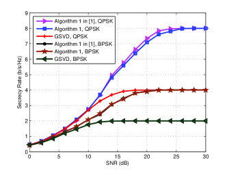
flushleft

Figure 1: Secrecy rate versus SNR for the $4\times 3\times 2$ wiretap channel for different precoder designs and different modulation schemes for $N_{s}=2$.

In Figure 2, we show the secrecy rate for the $64\times 48\times 48$ wiretap channel for different precoder designs and different modulation schemes for $N_{s}=2$. As indicated in Table II, the computational complexity of the precoder design in [1] is prohibitive in this case and no results can be shown. We observe that the secrecy rate of the GSVD design is lower than the upper bound given in Theorem 1. This is because for the GSVD design, as indicated in [11, Eq. (12)], only the non-zero subchannels of Bob which are stronger than the corresponding subchannels of Eve can be used for transmission. The $b_{i}$, $i=1,\ldots,s$, in (6) are in ascending order while the $e_{i}$, $i=1,\ldots,s$, in (7) are in descending order. Therefore, a large proportion of Bob’s non-zero subchannels may be abandoned by the GSVD design for large-scale MIMO channels. As a result, Algorithm 1 achieves significantly higher secrecy rates than the GSVD design.

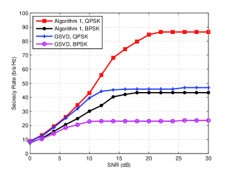
flushleft

Figure 2: Secrecy rate versus SNR for the $64\times 48\times 48$ wiretap channel for different precoder designs and different modulation schemes for $N_{s}=2$.

V Conclusion

In this paper, we have investigated the linear precoder design for large-scale MIMOME wiretap channels with finite alphabet signals. We derived an upper bound on the secrecy rate for the GSVD design in the high SNR regime. The derived expression reveals that the GSVD design may lead to a serious performance loss. Based on this, we proposed a PG-GSVD design to overcome the negative properties of the GSVD design while retaining an affordable computational complexity for large-scale MIMO systems. Simulations indicated that the proposed design performs well in large-scale MIMOME wiretap channels and achieves substantial secrecy rate gains compared to the GSVD design for finite alphabet inputs.

Appendix A Proof of Theorem 1

Based on (6) and (14), $I\left({{\mathbf{y}}_{b};{\mathbf{x}}_{a}}\right)$ in (5) for the GSVD design becomes

$$I\left({{{\bf{y}}_{b}};{{\bf{x}}_{a}}}\right)=\sum\limits_{i=1}^{s}{I\left({b_{i}^{2}{p_{k-r-s+i}}}\right)}+\sum\limits_{i=1}^{r}{I\left({{p_{k-s+i}}}\right)}$$ (39)

where $I(\gamma)=I(x;\sqrt{\gamma}x+n)$. Therefore, for $P\rightarrow\infty$, we obtain

$$\mathop{\lim}\limits_{P\to\infty}I\left({{{\bf{y}}_{b}};{{\bf{x}}_{a}}}\right)\leq(s+r)\log_{2}(M).$$ (40)

According to Inclusion–Exclusion Principle [20], we know

$${\rm dim}\left(\mathcal{S}_{ba}\right)+{\rm dim}\left(\mathcal{S}_{be}\right)={\rm dim}\left(\mathcal{S}_{ba}\cup\mathcal{S}_{be}\right)-{\rm dim}\left(\mathcal{S}_{ba}\cap\mathcal{S}_{be}\right).$$ (41)

For the subspaces $\mathcal{S}_{ba}$ and $\mathcal{S}_{be}$, we have

$$\mathcal{S}_{ba}\cap\mathcal{S}_{be}=$$

$$\left({\rm null}\left(\mathbf{H}_{ba}\right)^{\bot}\cap{\rm null}\left(\mathbf{H}_{ea}\right)\right)\cap\left({\rm null}\left(\mathbf{H}_{ba}\right)^{\bot}\cap{\rm null}\left(\mathbf{H}_{ea}\right)^{\bot}\right)$$ (42a)

$$=\left({\rm null}\left(\mathbf{H}_{ba}\right)^{\bot}\cap{\rm null}\left(\mathbf{H}_{ea}\right)\right)\cap\left({\rm null}\left(\mathbf{H}_{ea}\right)^{\bot}\cap{\rm null}\left(\mathbf{H}_{ba}\right)^{\bot}\right)$$ (42b)

$$={\rm null}\left(\mathbf{H}_{ba}\right)^{\bot}\cap\left(\left({\rm null}\left(\mathbf{H}_{ea}\right)\right)\cap{\rm null}\left(\mathbf{H}_{ea}\right)^{\bot}\right)\cap{\rm null}\left(\mathbf{H}_{ba}\right)^{\bot}$$ (42c)

$$=\varnothing$$ (42d)

where (42b) and (42c) are obtained based on the properties of intersections [21].

Also, we have

$$\mathcal{S}_{ba}\cup\mathcal{S}_{be}=$$

$$\left({\rm null}\left(\mathbf{H}_{ba}\right)^{\bot}\cap{\rm null}\left(\mathbf{H}_{ea}\right)\right)\cup\left({\rm null}\left(\mathbf{H}_{ba}\right)^{\bot}\!\cap\!{\rm null}\left(\mathbf{H}_{ea}\right)^{\bot}\right)\\$$ (43a)

$$={\rm null}\left(\mathbf{H}_{ba}\right)^{\bot}\cap\left({\rm null}\left(\mathbf{H}_{ea}\right)\cup{\rm null}\left(\mathbf{H}_{ea}\right)^{\bot}\right)$$ (43b)

$$={\rm null}\left(\mathbf{H}_{ba}\right)^{\bot}$$ (43c)

where (43b) and (43c) are obtained based on the Distributive Law of sets [21] and the Rank–Nullity Theorem [22], respectively.

From (41)–(43), we obtain

$$s+r={\rm dim}\left(\mathcal{S}_{ba}\right)+{\rm dim}\left(\mathcal{S}_{be}\right)={\rm dim}\left({\rm null}\left(\mathbf{H}_{ba}\right)^{\bot}\right).$$ (44)

Assuming $\mathbf{v}_{i}\in\mathbb{C}^{N_{t}\times 1}$ and $\mathbf{u}_{j}\in\mathbb{C}^{N_{r}\times 1}$ are the $N_{t}$ left and $N_{r}$ right singular vectors of $\mathbf{H}_{ba}$, respectively, $i=1,\ldots,N_{t}$, $j=1,\ldots,N_{r}$, $\mathbf{H}_{ba}$ can be written as

$$\mathbf{H}_{ba}=\sum\limits_{i=1}^{{N_{1}}}{{\lambda_{i}}{{\bf{u}}_{i}}{\bf{v}}_{i}^{H}}$$ (45)

where ${\lambda_{i}}$ is the singular value of $\mathbf{H}_{ea}$. For $N_{1}<N_{t}$, we have

$${\rm null}\left(\mathbf{H}_{ba}\right)=\sum\limits_{i=N_{1}+1}^{{N_{t}}}{{\omega_{i}}{{\bf{v}}_{i}}{\bf{v}}_{i}^{H}}$$ (46)

where ${\omega_{i}}$ denotes an arbitrary non-zero complex value, $i=1,\ldots,N_{t}$. Based on the property of the orthogonal complement of a subspace [23], we obtain

$$\left({\rm null}\left(\mathbf{H}_{ba}\right)^{\bot}\right)=\left(\sum\limits_{i=N_{1}+1}^{{N_{t}}}{{\omega_{i}}{{\bf{v}}_{i}}{\bf{v}}_{i}^{H}}\right)^{\bot}$$ (47a)

$$={\rm null}\left(\sum\limits_{i=N_{1}+1}^{{N_{t}}}{{\omega_{i}}{{\bf{v}}_{i}}{\bf{v}}_{i}^{H}}\right)$$ (47b)

$$=\sum\limits_{i=1}^{{N_{1}}}{{\omega_{i}}{{\bf{v}}_{i}}{\bf{v}}_{i}^{H}}.$$ (47c)

Therefore, we have

$${\rm dim}\left({\rm null}\left(\mathbf{H}_{ba}\right)^{\bot}\right)=N_{1}.$$ (48)

For $N_{1}=N_{t}$, ${\rm null}\left(\mathbf{H}_{ba}\right)=\varnothing$, and we obtain

$${\rm dim}\left({\rm null}\left(\mathbf{H}_{ba}\right)^{\bot}\right)=N_{t}.$$ (49)

Combining (5), (40), (44), (48), and (49) completes the proof.

Appendix B Proof of Theorem 2

The key idea of achieving the maximal rate $N_{t}\log M$ b/s/Hz in the high SNR regime is to guarantee that all $N_{t}$ signals can be received by Bob but not by Eve. To achieve this, $N_{s}$ signals are combined into a group and transmitted along the subchannels $\mathbf{R}_{r}$ in (24). As a result, we need to analyze the dimension of $\mathcal{S}_{ba}$.

Based on the Inclusion–Exclusion Principle [20], we have

$${\rm dim}\left(\mathcal{S}_{ba}\right)+{\rm dim}\left(\mathcal{S}_{n}\right)={\rm dim}\left(\mathcal{S}_{ba}\cup\mathcal{S}_{n}\right)-{\rm dim}\left(\mathcal{S}_{ba}\cap\mathcal{S}_{n}\right).$$ (50)

Following similar steps as in (42) and (43), we obtain

$$\mathcal{S}_{ba}\cap\mathcal{S}_{n}=$$

$$\left({\rm null}\left(\mathbf{H}_{ba}\right)^{\bot}\cap{\rm null}\left(\mathbf{H}_{ea}\right)\right)\cap\left({\rm null}\left(\mathbf{H}_{ba}\right)\cap{\rm null}\left(\mathbf{H}_{ea}\right)\right)$$ (51a)

$$=\left({\rm null}\left(\mathbf{H}_{ea}\right)\cap{\rm null}\left(\mathbf{H}_{ba}\right)^{\bot}\right)\cap\left({\rm null}\left(\mathbf{H}_{ba}\right)\cap{\rm null}\left(\mathbf{H}_{ea}\right)\right)$$ (51b)

$$={\rm null}\left(\mathbf{H}_{ea}\right)\!\cap\!\left(\left({\rm null}\left(\mathbf{H}_{ba}\right)\right)^{\bot}\cap{\rm null}\left(\mathbf{H}_{ba}\right)\right)\!\cap\!{\rm null}\left(\mathbf{H}_{ea}\right)$$ (51c)

$$=\varnothing$$ (51d)

and

$$\mathcal{S}_{ba}\cup\mathcal{S}_{n}=$$

$$\left({\rm null}\left(\mathbf{H}_{ba}\right)^{\bot}\cap{\rm null}\left(\mathbf{H}_{ea}\right)\right)\cup\left({\rm null}\left(\mathbf{H}_{ba}\right)\cap{\rm null}\left(\mathbf{H}_{ea}\right)\right)$$ (52a)

$$={\rm null}\left(\mathbf{H}_{ea}\right)\cap\left({\rm null}\left(\mathbf{H}_{ba}\right)^{\bot}\cup{\rm null}\left(\mathbf{H}_{ea}\right)\right)$$ (52b)

$$={\rm null}\left(\mathbf{H}_{ea}\right).$$ (52c)

Since ${\rm rank}\left(\mathbf{H}_{ea}\right)=N_{2}$, we have ${\rm dim}\left({\rm null}\left(\mathbf{H}_{ea}\right)\right)=N_{t}-N_{2}$. Then, based on (50), (51d), (52c), we obtain

$$r+N_{t}-k=N_{t}-N_{2}.$$ (53)

From (53), we know $r=k-N_{2}$.

When $(k-N_{2})N_{s}\geq N_{t}$, we design the PG-GSVD precoder in (28) as follows. We set

$$\mathbf{P}=\hbox{}\vbox{\kern 0.86108pt\hbox{$\kern 0.0pt\kern 2.5pt\kern-5.0pt\left[\kern 0.0pt\kern-2.5pt\kern-5.55557pt\vbox{\kern-0.86108pt\vbox{\vbox{ \halign{\kern\arraycolsep\hfil\@arstrut$\kbcolstyle#$\hfil\kern\arraycolsep& \kern\arraycolsep\hfil$\@kbrowstyle#$\ifkbalignright\relax\else\hfil\fi\kern\arraycolsep&& \kern\arraycolsep\hfil$\@kbrowstyle#$\ifkbalignright\relax\else\hfil\fi\kern\arraycolsep\cr 5.0pt\hfil\@arstrut$\scriptstyle~{}$\hfil\kern 5.0pt&5.0pt\hfil$\scriptstyle k-r-s$\hfil\kern 5.0pt&5.0pt\hfil$\scriptstyle s$\hfil\kern 5.0pt&5.0pt\hfil$\scriptstyle r$\hfil\kern 5.0pt&5.0pt\hfil$\scriptstyle N_{t}-k$\hfil\kern 5.0pt\crcr\kern 0.86108pt\cr 5.0pt\hfil\@arstrut$\scriptstyle k-r-s$\hfil\kern 5.0pt&5.0pt\hfil$\mathbf{0}$\hfil\kern 5.0pt&5.0pt\hfil$\mathbf{0}$\hfil\kern 5.0pt&5.0pt\hfil$\mathbf{0}$\hfil\kern 5.0pt&5.0pt\hfil$\mathbf{0}$\hfil\kern 5.0pt\cr 5.0pt\hfil\@arstrut$\scriptstyle s$\hfil\kern 5.0pt&5.0pt\hfil$\mathbf{0}$\hfil\kern 5.0pt&5.0pt\hfil$\mathbf{0}$\hfil\kern 5.0pt&5.0pt\hfil$\mathbf{0}$\hfil\kern 5.0pt&5.0pt\hfil$\mathbf{0}$\hfil\kern 5.0pt\cr 5.0pt\hfil\@arstrut$\scriptstyle r$\hfil\kern 5.0pt&5.0pt\hfil$\mathbf{0}$\hfil\kern 5.0pt&5.0pt\hfil$\mathbf{0}$\hfil\kern 5.0pt&5.0pt\hfil${\rm diag}\left(p_{1},\ldots p_{r}\right)$\hfil\kern 5.0pt&5.0pt\hfil$\mathbf{0}$\hfil\kern 5.0pt\cr 5.0pt\hfil\@arstrut$\scriptstyle N_{t}-k$\hfil\kern 5.0pt&5.0pt\hfil$\mathbf{0}$\hfil\kern 5.0pt&5.0pt\hfil$\mathbf{0}$\hfil\kern 5.0pt&5.0pt\hfil$\mathbf{0}$\hfil\kern 5.0pt&5.0pt\hfil$\mathbf{0}$\hfil\kern 5.0pt\cr}}}}\right]$}}.$$ (54)

Also, we select a pairing scheme $\left\{\ell_{1},\ldots,\ell_{N_{t}}\right\}$ in (29) satisfying

$$\left[\mathbf{P}_{s}\right]_{ii}=\\ \left\{\begin{array}[]{l}0\quad\quad\quad{\rm if}\ 1\leq i\leq N_{s}-1\\ \frac{p_{j}}{\omega_{k-r+j}}\ \,{\rm if}\ i=N_{s}\end{array}\right.$$ (55)

for $s=1,\ldots,S$, $i=1,\ldots,N_{s}$, and $j=1,\ldots,r$.

Based on the design in (54) and (55), in the high SNR regime, we have

$$I\left({{\bf{y}}_{b,s}};\mathbf{x}_{s}\right) \mathop{\to}\limits^{P\to\infty}N_{s}\log M$$ (56)

$$I\left({{\bf{y}}_{e,s}};\mathbf{x}_{s}\right) =0.$$ (57)

Substituting (56) and (57) into (38) completes the proof.

References

• [1] Y. Wu, C. Xiao, Z. Ding, X. Gao, and S. Jin, “Linear precoding for finite-alphabet signaling over MIMOME wiretap channels,” IEEE Trans. Veh. Technol., vol. 61, pp. 2599–2612, Jul. 2012.
• [2] A. D. Wyner, “The wiretap channel,” Bell Syst. Tech. J., vol. 54, pp. 1355–1387, Oct. 1975.
• [3] A. Khisti and G. W. Wornell, “Secure transmission with multiple antennas-Part II: The MIMOME wiretap channel,” IEEE Trans. Inf. Theory, vol. 56, pp. 5515–5532, Nov. 2010.
• [4] M. C. Gursoy, “Secure communication in the low-SNR regime,” IEEE Trans. Commun., vol. 60, pp. 1114–1123, Apr. 2012.
• [5] W. Zeng, Y. R. Zheng, and C. Xiao, “Multi-antenna secure cognitive radio networks with finite-alphabet inputs: A global optimization approach for precoder design,” IEEE Trans. Wireless Commun., vol. 15, pp. 3044–3057, Apr. 2016.
• [6] Y. Wu, R. Schober, D. W. K. Ng, C. Xiao, and G. Caire, “Secure massive MIMO transmission with an active eavesdropper,” IEEE Trans. Inf. Theory, vol. 62, pp. 3880–3900, Jul. 2016.
• [7] A. Lozano, A. M. Tulino, and S. Verdú, “Optimum power allocation for parallel Gaussian channels with arbitrary input distributions,” IEEE Trans. Inform. Theory, pp. 3033–3051, Jul. 2006.
• [8] C. Xiao, Y. R. Zheng, and Z. Ding, “Globally optimal linear precoders for finite alphabet signals over complex vector Gaussian channels,” IEEE Trans. Signal Process., pp. 3301–3314, Jul. 2011.
• [9] Y. Wu, S. Jin, X. Gao, C. Xiao, and M. R. McKay, “MIMO multichannel beamforming in Rayleigh-product channels with arbitrary-power co-channel interference and noise,” IEEE Trans. Wireless Commun., vol. 3, pp. 3677–3691, Oct. 2012.
• [10] Y. Wu, C. Xiao, X. Gao, J. Matyjas, and Z. Ding, “Linear precoder design for MIMO interference channels with finite-alphabet signaling,” IEEE Trans. Commun., vol. 61, pp. 3766–3780, Sep. 2013.
• [11] S. Bashar, Z. Ding, and C. Xiao, “On secrecy rate analysis of MIMO wiretap channels driven by finite-alphabet input,” IEEE Trans. Commun., vol. 60, pp. 3816–3825, Dec. 2012.
• [12] S. R. Aghdam and T. M. Duman, “Low complexity precoding for MIMOME wiretap channels based on cut-off rate,” in Proc. IEEE Int. Symp. Inf. Theory (ISIT’2016), Barcelona, Spain, Jul. 2016, pp. 2988–2992.
• [13] Y. Wu, C.-K. Wen, C. Xiao, X. Gao, and R. Schober, “Linear precoding for the MIMO multiple access channel with finite alphabet inputs and statistical CSI,” IEEE Trans. Wireless Commun., vol. 14, pp. 983–997, Feb. 2015.
• [14] T. L. Marzetta, “Noncooperative cellular wireless with unlimited numbers of base station antennas,” IEEE Trans. Wireless Commun., vol. 15, pp. 3590–3600, Nov. 2010.
• [15] E. G. Larsson, O. Edfors, F. Tufvesson, and T. L. Marzetta, “Massive MIMO for next generation wireless systems,” IEEE Commun. Mag., vol. 52, pp. 186–195, Feb. 2014.
• [16] S. K. Mohammed, E. Viterbo, Y. Hong, and A. Chockalingam, “Precoding by pairing subchannels to increase MIMO capacity with discrete input alphabets,” IEEE Trans. Inform. Theory, pp. 4156–4169, Jul. 2011.
• [17] T. Ketseoglou and E. Ayanoglu, “Linear precoding for MIMO with LDPC coding and reduced complexity,” IEEE Trans. Wireless Commun., pp. 2192–2204, Apr. 2015.
• [18] Y. Wu, D. W. K. Ng, C. W. Wen, R. Schober, and A. Lozano, “Low-complexity MIMO precoding with discrete signals and statistical CSI,” in Proc. IEEE Int. Telecommun. Conf. (ICC’2016), Kuala Lumpur, Malaysia, May 2016, pp. 1–6.
• [19] D. P. Palomar and S. Verdú, “Gradient of mutual information in linear vector Gaussian channels,” IEEE Trans. Inform. Theory, vol. 52, pp. 141–154, Jan. 2006.
• [20] G. E. Andrews, Number Theory.   Philadelphia, PA: Saunders, 1971.
• [21] R. P. Halmos, Naive Set Theory.   New Jersey: Van Nostrand, 1960.
• [22] S. Banerjee and A. Roy, Linear Algebra and Matrix Analysis for Statistics.   London: Chapman and Hall/CRC, 2014.
• [23] R. P. Halmos, Finite-dimensional vector spaces.   New York: Springer-Verlag, 1974.