A model for stealth coronal mass ejections

Abstract

Stealth coronal mass ejections (CMEs) are events in which there are almost no observable signatures of the CME eruption in the low corona but often a well-resolved slow flux rope CME observed in the coronagraph data. We present results from a three-dimensional numerical magnetohydrodynamics (MHD) simulation of the 1–2 June 2008 slow streamer blowout CME that Robbrecht et al. (2009) called “the CME from nowhere.” We model the global coronal structure using a 1.4 MK isothermal solar wind and a low-order potential field source surface representation of the Carrington Rotation 2070 magnetogram synoptic map. The bipolar streamer belt arcade is energized by simple shearing flows applied in the vicinity of the helmet streamer’s polarity inversion line. The flows are large scale and impart a shear typical of that expected from the differential rotation. The slow expansion of the energized helmet streamer arcade results in the formation of a radial current sheet. The subsequent onset of expansion-induced flare reconnection initiates the stealth CME while gradually releasing the stored magnetic energy. We present favorable comparisons between our simulation results and the multiviewpoint SOHO-LASCO (Large Angle and Spectrometric Coronagraph) and STEREO-SECCHI (Sun Earth Connection Coronal and Heliospheric Investigation) coronagraph observations of the preeruption streamer structure and the initiation and evolution of the stealth streamer blowout CME.

1 Introduction

Stealth coronal mass ejections (CMEs) are CME events with virtually no identifiable surface or low corona signatures that indicate an eruption has occurred. The stereoscopic viewing and improvements in heliospheric white-light imaging by STEREO Sun Earth Connection Coronal and Heliospheric Investigation (SECCHI) instruments, combined with the last solar minimum’s exceptionally low activity levels, have dramatically increased the number and proportion of events now classified as stealth CMEs. This is partly due to more eruptive transients being classified as CMEs, fewer fast CMEs during the early years of the STEREO mission and the stereoscopic viewing being able to rule out events that would have been previously classified as “backside halo CMEs” (Howard and Harrison, 2013). Whether stealth CMEs constitute a distinct class of CME event in their own right or merely represent a subset of a more common or universal set of CME phenomena is still under debate. Stealth CMEs have a particular relevance for space weather forecasting as potentially geoeffective interplanetary CME (ICME) structures that lack the usual solar eruption warning signs.

Howard and Harrison (2013) presented a historic perspective of the stealth CME phenomena and argue that they are, in fact, merely the subset of slow, streamer blowout type of CMEs (Sheeley et al., 2007) that have been seen since Skylab. Ma et al. (2010) conducted a statistical study of stealth CME events and concluded their eruption velocities in the coronagraph fields of view were consistent with—and essentially defined—the low end of the CME speed distribution ($\lesssim 300$ km s^-1). Pevtsov et al. (2012) examined properties of the solar source regions for several slow- to moderate-speed CME events that originated in “empty” filament channels, i.e. long polarity inversion lines in the underlying photospheric magnetic field distribution with highly sheared coronal magnetic fields but no discernible filament or prominence material. D’Huys et al. (2014) followed up on the study by Ma et al. (2010) by presenting a set of $\sim$40 stealth CME events. Alzate and Morgan (2016) have shown that with sufficiently advanced image-processing techniques and the extended field of view of the PROBA2 coronagraph, the vast majority of the D’Huys et al. (2014) stealth CME events do, in fact, have some low coronal signatures. These findings confirm our main conclusion here, that stealth CMEs are not a new, mysterious, and unknown eruptive phenomena.

Robbrecht et al. (2009) analyzed the STEREO observations of the 1–2 June 2008 stealth CME eruption. The STEREO viewpoint geometry was such that the CME was a near-perfect limb event in STEREO-A coronagraph and heliospheric imager observations and was directed toward STEREO-B. The in situ STEREO-B plasma and magnetic field observations showed classic flux rope ICME signatures at 1 AU. Therefore, there have been a number of detailed studies of various aspects of this CME-ICME event that link the remote and in-situ measurements (e.g. Robbrecht et al., 2009; Möstl et al., 2009; Bisi et al., 2010; Lynch et al., 2010; Wood et al., 2010; Nieves-Chinchilla et al., 2011, 2012; Rodriguez et al., 2011; Rollett et al., 2012).

There are several competing models for the initiation of coronal mass ejections and several competing mechanisms for the gradual accumulation of the free magnetic energy necessary for release during the eruption (e.g., see reviews by Klimchuk, 2001; Forbes et al., 2006; Aulanier, 2014; Janvier et al., 2015, and references therein). In general, regardless of the specific ideal or resistive magnetohydrodynamic (MHD) instabilities associated with the rapid transition to a catastrophic, run-away eruption of coronal fields and plasma, essentially every CME model leads to magnetic reconnection at a vertical/radial current sheet that drives the eruption in the manner of the CSHKP eruptive flare scenario (Carmichael, 1964; Sturrock, 1966; Hirayama, 1974; Kopp and Pneuman, 1976).

One of the simplest ways to model the energization of a magnetic field arcade in MHD simulations is through the gradual shearing of the arcade foot points parallel to the polarity inversion line of the magnetic configuration (DeVore and Antiochos, 2000). Mikić and Linker (1994) showed that given sufficient energization, a spherical, axisymmetric sheared dipole arcade could create such an extended radial current sheet so that, eventually, magnetic reconnection would facilitate the rapid formation of a disconnected flux rope that is ejected out of the simulation domain. Linker and Mikić (1995) repeated this form of driving in an axisymmetric bipolar helmet streamer configuration and showed the presence of a background solar wind increased the energy of the erupting structure. A fully 3-dimensional (3-D), spherical version of a sheared arcade eruption was presented by Linker et al. (2003).

In the MHD simulation results presented here, we utilize this same basic energization mechanism—the slow gradual shearing of a 3-D helmet streamer arcade in a simple isothermal solar wind—and model the evolution and eruption of a slow, streamer blowout-type CME that reproduces many of the observational properties of the 1–2 June 2008 STEREO stealth CME event. Our results strongly support the Howard and Harrison (2013) conjecture that stealth CMEs are not fundamentally different than most slow CME eruptions but just represent the lowest-energy range of the CME distribution.

The paper is organized as follows. In section 2 we describe the numerical methods and the MHD simulation setup, including the computational grid and boundary conditions, initial potential field source surface configuration derived from the observed magnetograph synoptic map, the isothermal wind model and its relaxation to steady state. We then compare the global, quasi-steady state model streamer structure to multispacecraft coronagraph observations. In section 3 we present the simulation results. First, we describe the shear flows used to energize the bipolar helmet streamer arcade, then we present the global energy evolution of the system and examine the stealth CME initiation, and finally we examine the magnetic field structure and evolution of the CME flux rope as it forms and propagates, including its dynamics through the coronagraph field of view. In section 4 we discuss the implications of our modeling results for CME initiation and global coronal evolution and for space weather forecasting. In section 5 we summarize our results and present the conclusions.

2 Numerical Simulation Setup

2.1 ARMS Model Description

The Adaptively Refined MHD Solver (ARMS) (DeVore and Antiochos, 2008) calculates solutions to the 3-D nonlinear, time-dependent MHD equations that describe the evolution and transport of density, momentum, and energy throughout the plasma, and the evolution of the magnetic field and electric currents using a finite-volume, multidimensional flux-corrected transport numerical scheme (DeVore, 1991). The ARMS code is fully integrated with the adaptive mesh toolkit PARAMESH (MacNeice et al., 2000) to handle solution-adaptive grid refinement and support efficient multiprocessor parallelization. ARMS has been used to perform a wide variety of numerical simulations of dynamic phenomena in the solar atmosphere, including 3-D magnetic breakout CME initiation (DeVore and Antiochos, 2008; Lynch et al., 2008) and ejecta propagation through the low corona (Lynch et al., 2009).

For our simulation, we use ARMS to solve the ideal MHD equations in spherical coordinates,

$$\frac{\partial\rho}{\partial t}+\nabla\cdot\left(\rho\boldsymbol{v}\right)=0,$$ (1)

$$\frac{\partial}{\partial t}\left(\rho\boldsymbol{v}\right)+\nabla\cdot\left(\rho\boldsymbol{v}\boldsymbol{v}\right)+\nabla P=\frac{1}{4\pi}\left(\nabla\times\boldsymbol{B}\right)\times\boldsymbol{B}-\rho\boldsymbol{g},$$ (2)

$$\frac{\partial\boldsymbol{B}}{\partial t}=\nabla\times\left(\boldsymbol{v}\times\boldsymbol{B}\right),$$ (3)

where all the variables retain their usual meaning, solar gravity is $\boldsymbol{g}=g_{\odot}(r/R_{\odot})^{-2}\boldsymbol{\hat{r}}$ with $g_{\odot}=2.75\times 10^{4}$ cm s^-2, and we use the ideal gas law $P=2(\rho/m_{p})k_{B}T$. However, given the isothermal model used in the construction of our background solar wind, we do not solve an internal energy or temperature equation. The plasma temperature remains uniform throughout the domain for the duration of the simulation. Since coronal plasma is highly conductive and the dominant heat flux is carried by fast-moving electrons, the isothermal assumption of an “infinite conductivity” is a reasonable approximation.

Additionally, while there is no explicit magnetic resistivity in the equations of ideal MHD, necessary and stabilizing numerical diffusion terms introduce an effective resistivity on very small spatial scales, i.e., the size of the grid. In this way, magnetic reconnection can occur when current sheet features and the associated gradients of field reversals have been distorted and compressed to the local grid resolution scale.

The spherical computational domain uses logarithmic grid spacing in $r$ and uniform grid spacing in $\theta,\phi$. The domain extends from $r\in\left[1R_{\odot},30R_{\odot}\right]$, $\theta\in\left[0.0625\pi,0.9375\pi\right]$, and $\phi\in\left[-\pi,\pi\right]$. The initial grid consists of $8\times 7\times 16$ blocks with 8³ grid cells per block. There are 2 additional levels of static grid refinement: the level 2 refinement covers $r\leq 3.58R_{\odot}$ for $\phi\in\left[-0.1875\pi,\pi\right]$ and all $\theta$; the level 3 refinement is over $r\leq 3.58R_{\odot}$ for $\phi\in\left[-\pi,-0.1875\pi\right]$ for all $\theta$ and includes an additional spherical wedge through $30R_{\odot}$ from $\theta\in\left[0.375\pi,0.750\pi\right]$ and $\phi\in\left[-0.9375\pi,-0.3125\pi\right]$, encompassing the volume above the streamer blowout eruption.

Figure 1 shows the computational block structure. Figure 1a plots the equatorial $(r,\phi)$ plane. The angular positions of the STEREO-B (blue square; $\phi_{\rm STB}=-101.9^{\circ}$), SOHO (green diamond; $\phi_{\rm SOHO}=-77.0^{\circ}$), and STEREO-A (red triangle; $\phi_{\rm STA}=-48.4^{\circ}$) spacecraft on 2 June 2008 are also shown (converted from Carrington Longitude to the ARMS coordinate system). The STB, SOHO, and STA planes of sky are plotted as the solid lines. Figure 1b plots the block structure in the $(r,\theta)$ plane corresponding to the east limb of STA plane of sky. Figure 1c plots the zoomed-in view of inner corona for the STA plane of sky. This grid structure yields a modest resolution of $\sim$$1.6\times 10^{4}$ leaf blocks and $\sim$$8.2\times 10^{6}$ computational grid cells. The highest refinement region on the east limb corresponds to a global grid size of $256\times 224\times 512$ in $({\log r},\theta,\phi)$, a radial resolution of 0.0134$R_{\odot}$ at $r=1R_{\odot}$, and an angular resolution of $0.703^{\circ}\times 0.703^{\circ}$.

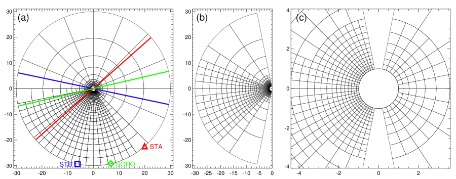
Figure 1: The 3-D spherical $\log{r}$ computational block structure. (a) The $r$-$\phi$ plane with the relative heliographic longitude separation of the STEREO and SOHO spacecraft on 2 June 2008 (labeled plot symbols) as well as their respective plane-of-the-sky orientations (STA–red; SOHO–green; STB–blue). (b) The $r$-$\theta$ plane corresponding to the east limb viewpoint of STEREO-A. (c) A zoomed-in view of the static block refinement near the Sun in Figure 1b.

The simulation’s boundary conditions are the following. The left and right $\phi$ boundaries are periodic. The left and right $\theta$ boundaries are closed, which sets all fluxes across the boundary to zero. The left (bottom) and right (top) radial boundary conditions are set to allow the implementation of our solar wind solution described in section 2.3. The guard cells of the radial boundaries are filled symmetrically, and both the inner and outer boundaries are open to fluxes of all quantities. The inner $r$ boundary guard cells are filled with values of the initial atmospheric density, pressure, and temperature at every time step, but the velocities in the guard cells are set to zero. This creates a passive absorbing layer in which the normal flows across the boundary arise via the averaging to obtain the value at the cell face. These flows compensate for the differences in density/pressure that develop during the evolution of the system. This absorbing layer also acts as an effective mass source which is necessary to maintain a quasi-steady state solar wind outflow. The outer $r$ boundary guard cells are filled with the solution at the edge of the domain multiplied by a factor corresponding to the radial dependence of the initial atmospheric profile. The outer radial boundary allows flow through in the same manner as the inner boundary. Since the quasi-steady state solar wind outflow is supersonic and super-Alfvénic by 30$R_{\odot}$, the influence of the outer boundary conditions on the simulation is minimal.

2.2 Initial Magnetic Field

We initialize the ARMS simulation magnetic field with the potential field source surface (PFSS) reconstruction (e.g., Wang and Sheeley, 1992; Luhmann et al., 1998) of the SOHO-MDI (Scherrer et al., 1995) polar-corrected synoptic map data (Liu et al., 2007) for Carrington Rotation 2070 with the source surface set to 2.5$R_{\odot}$. Robbrecht et al. (2009) and Lynch et al. (2010) estimated the 1–2 June 2008 stealth CME source region as a large swath of the helmet streamer belt, so here we can use a low-order PFSS $(\ell_{\rm max}=9)$ extrapolation and still capture the overall structure of the helmet streamer.

Figure 2 plots the SOHO/MDI data and the initial $r=R_{\odot}$ magnetic field used in the MHD simulation. Figure 2a shows the MDI full disk magnetogram at 01:39UT on 2 June 2008 and Figure 2b plots the CR2070 synoptic map. Here the CME source region estimate by Robbrecht et al. (2009) is indicated in the orange box and the positions of STEREO-B, SOHO, and STEREO-A are shown as blue, green, and red vertical lines at their respective Carrington longitudes. Figure 2c plots the full disk SOHO view of the ARMS radial magnetic field and panel (d) plots the PFSS representation of the simulation’s $B_{r}(R_{\odot},\theta,\phi)$ synoptic map. The magenta contours represent the polarity inversion lines in the PFSS field. The magnetic configuration of the 1–2 June 2008 CME source region becomes apparent as the large scale polarity inversion line corresponding to the main helmet streamer belt.

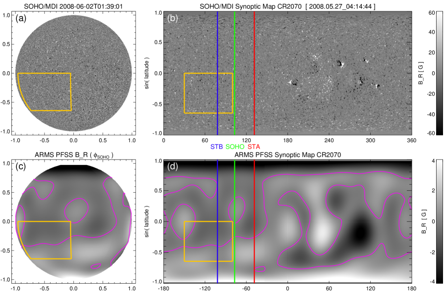
Figure 2: The observed photospheric and model coronal fields. (a) SOHO-MDI magnetogram on 2 June 2008. The Robbrecht et al. (2009) estimate of the stealth CME source region is shown as the yellow region. (b) MDI synoptic map for CR2070. The respective spacecraft longitudes are shown as vertical lines (STA–red; SOHO–green; STB–blue). (c) ARMS simulation radial field distribution from SOHO/L1 viewpoint. The $B_{r}=0$ polarity inversion lines are plotted in magenta. (d) Low-order PFSS representation of the CR2070 synoptic map.

2.3 Isothermal Solar Wind Solution

The solar wind is initialized in ARMS by first solving the one-dimensional Parker (1958) equation for an isothermal coronal atmosphere,

$$\frac{v_{\rm sw}^{2}}{c_{0}^{2}}-\ln\left(\frac{v_{\rm sw}^{2}}{c_{0}^{2}}\right)=-3+4\ln\left(\frac{r}{r_{c}}\right)+4\frac{r_{c}}{r},$$ (4)

where the base number density, pressure, and temperature are $n_{0}=\rho_{0}/m_{p}=1.29\times 10^{8}$ cm^-3, $P_{0}=0.05$ dyn cm^-2, and $T_{0}=1.40\times 10^{6}$ K, respectively. Here, $c_{0}=(2k_{B}T_{0}/m_{p})^{1/2}=152$ km s^-1 is the thermal velocity at $T_{0}$, the location of the critical point is $r_{c}=GM_{\odot}/2c_{0}^{2}=4.10R_{\odot}$. This yields a solar wind speed at the outer boundary of $v_{\rm sw}(30R_{\odot})\sim 450$ km s^-1.

At time $t=0$ s we impose this Parker $v_{\rm sw}(r)$ profile and use it to set the initial mass density profile $\rho(r)$ from the steady mass-flux condition ($\rho v_{\rm sw}r^{2}=$ constant) throughout the computational domain. The $v_{\rm sw}(r)$ profile is shown as the contour plane in Figure 3a alongside representative magnetic field lines of the initial PFSS magnetic field model. We then let the system relax for $t=2.16\times 10^{5}$ s (60 h) and Figure 3b shows a snapshot of the magnetic field and radial velocity at the end of the relaxation phase (this figure is available as an animation in the supporting information of this article). The initial discontinuities in the magnetic field at the source surface ($r=2.5R_{\odot}$) propagate outwards and eventually through the outer boundary. The Figure 3 animation shows that the dragging of some of the closed streamer belt flux by the solar wind flow sets up the condition for the transverse pressure from the open fields to push in behind the expanding streamer belt structure forming the elongated current sheet. Eventually, the numerical diffusion allows magnetic reconnection between the elongated streamer belt field lines and gives the system the opportunity to adjust the amount of open flux relative to the new pressure balance associated with the background solar wind flows, as seen in Figure 3b. The inner boundary mass source allows material to accumulate in the closed field regions and sets up steady radial flows along open field lines.

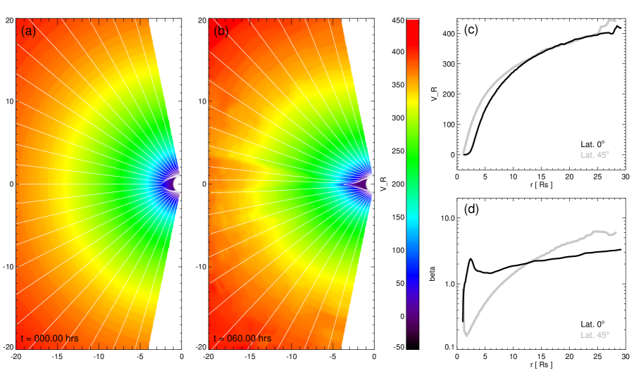
Figure 3: The relaxation of the isothermal solar wind solution. (a) The initial Parker $v_{\rm sw}(r)$ solution with representative field lines illustrating the initial PFSS magnetic field solution for the STA east limb viewpoint. (b) The same quantities at the end of the relaxation phase ($t=60$ h). (c) Two radial cuts through the $V_{r}(r,\theta)$ simulation data shown in Figure 3b, one at the equator (black) going through the helmet streamer, and the other at +45^∘ (gray) sampling the polar coronal hole. (d) Radial cuts for plasma $\beta=8\pi P/B^{2}$. An animation of the solar wind relaxation (Figures 3a and 3b) is available as supporting information of the article.

Our isothermal solar wind never actually achieves a true “steady state” stationary outflow. We see a continuous, dynamic situation of small-scale opening and closing at the Y point of the streamer belt and in the heliospheric current sheet. In simulations with much higher resolution (e.g., see Allred and MacNeice, 2015), interchange reconnection and the intermittent generation of magnetic islands in the heliospheric current sheet are likely one of the sources of the well-known “streamer blob” intensity enhancements that have been shown to passively advect with the slow solar wind (Sheeley et al., 1997; Wang et al., 2000).

2.4 Global Preeruption Coronal Structure

We have constructed synthetic total brightness images $I(t)$ from the ARMS simulation data by building 2-D plane-of-sky images where each pixel corresponds to a line-of-sight integration of white-light intensity associated with Thomson scattering from the 3-D density data (as in Vourlidas et al., 2013). The white-light scattering is calculated with a Fortran implementation of the SolarSoft routine eltheory.pro, where the intensity contribution from the simulation density along the line of sight is determined by the observing geometry (Billings, 1966; Vourlidas and Howard, 2006). In order to mimic the coronagraph analysis procedures, we construct “ratio images” from the white-light intensity images (see Sheeley et al., 1997). The $I(t)/I(0)$ ratio compensates for the (spherically symmetric, background) density profile’s radial dependence and thus highlights the extended streamer structures. The ratio images are equivalent to performing background subtraction for logarithmic intensity scales.

Figure 4 (top row) shows the preeruption coronal structure as observed by multiple coronagraph instruments from the STB (left), SOHO (middle), and STA (right) viewpoints. Each of the STEREO viewpoints includes observations from the COR1 and COR2 cameras from the SECCHI suite and are supplemented by the averaged MK4 coronagraph data on 1 June 2008 from the Mauna Loa Solar Observatory. The MK4 data are time shifted by approximately 2 days with respect to each of the STEREO image composites ($\sim$26^∘ in Carrington longitude) but still show reasonable agreement with the extended COR1 and COR2 large-scale helmet streamer structures. The SOHO viewpoint data come from the SOHO/Large Angle Spectrometric Coronagraph (LASCO) C2 instrument and are likewise supplemented by the MK4 data. Here the 195 Å EUV emission over the disk is also shown from the STEREO EUVI and SOHO EIT instruments. Figure 4 (bottom row) plots the white-light intensity ratio images from the $(\phi_{\rm STB},\phi_{\rm SOHO},\phi_{\rm STA})$ perspectives at $t=60$ h with color scales chosen to correspond to the different coronagraph observations used above. For each of the three spacecraft perspectives, we capture the large-scale coronal streamer and pseudostreamer structures seen in the observations.

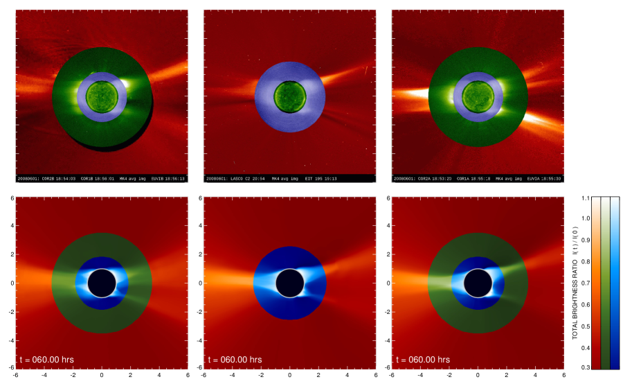
Figure 4: Multispacecraft coronagraph observations and model results of the preeruption streamer structure. (top row) (left) STB, (middle) SOHO, and (right) STA observations supplemented with averaged MK4 data from 1 June 2008. (bottom row) Synthetic white-light emission ratio images of the steady state coronal streamer structure at the end of the relaxation phase ($t=60$ h) from the STB, SOHO, and STA viewpoints.

3 MHD Simulation Results

3.1 Shearing the Bipolar Helmet Streamer Arcade With Boundary Flows

The helmet streamer is energized via ideal foot point shearing flows imposed at the $r=R_{\odot}$ boundary, roughly parallel to the polarity inversion line (PIL) in the CME source region. Here we define

$$\boldsymbol{V}_{\rm shear}(\theta,\phi,t)=V_{0}\left[\sum_{i=1}^{4}\Theta^{i}(\theta)\Phi^{i}(\phi)\right]T(t)\boldsymbol{\hat{\phi}}.$$ (5)

The separable spatial dependence functions are of the form

$$\Theta^{i}(\theta)=\sin{\left[2\pi k^{i}_{\theta}\frac{(\theta-\theta^{i}_{C})}{(\theta^{i}_{L}-\theta^{i}_{R})}\right]}\;,$$ (6)

$$\Phi^{i}(\phi)=\frac{1}{2}-\frac{1}{2}\cos{\left[2\pi k^{i}_{\phi}\frac{(\phi-\phi^{i}_{C})}{(\phi^{i}_{L}-\phi^{i}_{R})}\right]},$$ (7)

and the temporal dependence is

$${\rm T}(t)=\frac{1}{2}-\frac{1}{2}\cos{\left[2\pi\frac{(t-60)}{20}\right]}.$$ (8)

Each of the separable functions above is defined only for $\theta\in[\theta^{i}_{L},\theta^{i}_{R}]$, $\phi\in[\phi^{i}_{L},\phi^{i}_{R}]$ with respective phase shifts ($\theta^{i}_{C}$, $\phi^{i}_{C}$), for $t\in\left[60,80\right]$ h and are zero elsewhere. Table 1 lists each of the specific parameters for the four flow fields $(i=1,4)$ that make up the composite shearing profile. We have chosen $V_{0}=30$ km s^-1 so that the spatial and temporal average of the composite profile yields a mean velocity magnitude of $\sim$3.50 km s^-1 in each magnetic polarity over the 20 h duration. Although the maximum shearing velocity $V_{0}$ is roughly 30 times the magnitude of typical photospheric velocities, it is less than both the sound speed $(V_{0}/c_{0}\sim 20\%)$ and the Alfvén speed $(V_{0}/\langle V_{A}\rangle\sim 15\%)$ in the helmet streamer region near the lower radial boundary. Thus, the system evolves quasi-statically.

We generate a total foot point displacement of $\approx 2.6\times 10^{5}$ km ($\sim 0.37R_{\odot}$) in each polarity over the 20 h temporal duration of the applied shearing flows. This corresponds to roughly the same foot point displacement that would occur over 15 days of differential rotation using the Lynch et al. (2010) estimate of 0.20 km s^-1 in the $\phi$-direction over the 40^∘ latitudinal extent of the source region.

Table 1: Parameters for the Spatial Extent of the Surface Shearing Profile Given by Equation (5).

$i$	$k_{\theta}$	$\theta_{L}$ (deg)	$\theta_{R}$ (deg)	$\theta_{C}$ (deg)	$k_{\phi}$	$\phi_{L}$ (deg)	$\phi_{R}$ (deg)	$\phi_{C}$ (deg)
1	0.25	94.0	108.25	94.0	1.0	-130.0	-40.0	-85.0
2	-0.25	108.25	111.75	111.75	1.0	-130.0	-40.0	-85.0
3	0.25	113.75	117.25	113.75	1.0	-150.0	-60.0	-105.0
4	-0.25	117.25	129.75	129.75	1.0	-150.0	-60.0	-105.0

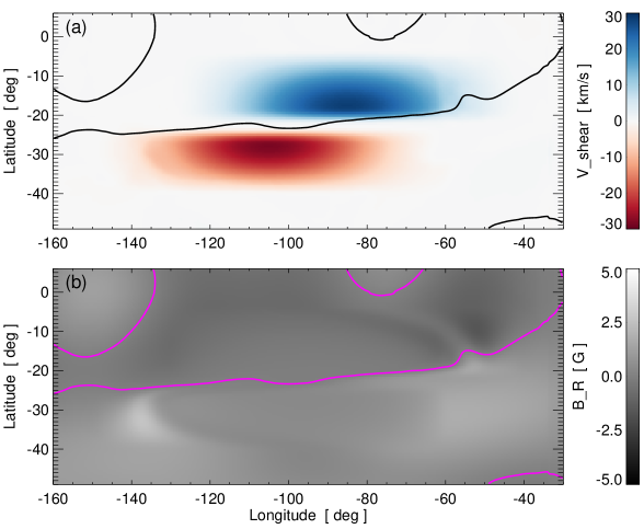
Figure 5: (a) The maximum shearing velocity $\boldsymbol{V}_{\rm shear}(t=70~{}{\rm h})$ on the $r=R_{\odot}$ boundary. (b) The corresponding $B_{r}(R_{\odot},\theta,\phi)$ distribution at $t=70$ h. The polarity inversion lines ($B_{r}=0$ contours) are shown as black (Figure 5a) and magenta (Figure 5b) lines.

Figure 5 plots the spatial extent of the shearing flow profile imposed at the $r=R_{\odot}$ lower boundary. Figure 5 (top) shows $\boldsymbol{V}_{\rm shear}(\theta,\phi,t=70{\rm\;h})$ corresponding to the time of the maximum shearing velocities. Figure 5 (bottom) plots the corresponding $B_{r}(\theta,\phi,t)$ distribution at the lower boundary. The $B_{r}=0$ magnetic PILs are shown in Figure 5 (top) (Figure 5, bottom) panel as black (magenta) contours. The imposed boundary flows alter the $B_{r}$ distribution, concentrating the negative and positive polarity radial flux, but the field strengths remain low over the region, i.e., $B_{r}\in[-5,+5]$ G. Because the shearing flows alter the PIL, there is a small amount of flux cancelation during the shearing phase and afterwards due to numerical diffusion. We have calculated the radial flux in the region depicted in Figure 5 and find the magnitudes of the positive and negative radial fluxes decrease by less than 2% during the shearing phase ($60\leq t\leq 80$ h) and less than 0.5% for $t>100$ h. We also note that the Linker et al. (2003) simulations of flux cancelation CME initiation typically required a $>10$% decrease in the radial flux in order to erupt.

Our applied boundary flows are large scale in order to capture the effect of shearing by differential rotation, and consequently, they do not result in the formation of a filament channel. This is a key difference between our stealth CME (and perhaps all streamer blowout CMEs) and the standard fast CME events originating in active regions that are considered by most CME models (e.g., Forbes et al., 2006). In one class of CME models the filament channel is presumed to be a twisted flux rope that becomes ideally unstable. As will be evident below, there is no structure in our preeruption corona that resembles a flux rope; the whole closed field system is sheared and there is no significant flux cancelation. This makes it highly unlikely that ideal mechanisms such as the kink or torus instability play a role in the ensuing eruption.

The simulation presented here also differs from the Lynch et al. (2009) simulation of 3-D magnetic breakout CME initiation. The source region field configuration in Lynch et al. (2009) had higher field strengths ($\pm 25$ G) and the shearing flows were more compact with respect to the active region (AR) PIL. The main topological difference is in the structure of the background field. In Lynch et al. (2009), the background fields were a global-scale, closed field dipole above an oppositely oriented AR bipole resulting in a source region with a true multipolar topology defined by a 3-D coronal null point and a separatrix dome surface between the two closed flux systems. Here, our 3-D helmet streamer is a traditional bipolar arcade flux system with a topological Y point (line) at the interface between the closed streamer flux and open flux from polar coronal holes. The Lynch et al. (2009) configuration was an idealized representation of a complex, multipolar AR source, whereas here our stealth CME originates from a slightly less idealized representation of the large-scale streamer belt above a quiet-Sun bipolar flux distribution.

Our initial PFSS representation of the large-scale coronal magnetic field for Carrington Rotation 2070 does not contain any of the necessary free magnetic energy to power the streamer blowout CME. One could, in principle, start with an earlier Carrington Rotation synoptic map and apply flux transport models (e.g. Wang et al., 1989; Schrijver, 2001) to the entire surface. Variations of this procedure have been used to successfully drive magnetofrictional modeling of coronal evolution over a wide range of spatial and temporal scales (see van Ballegooijen et al., 1998; Yeates and Mackay, 2009; Cheung and DeRosa, 2012). However, it would be wholly impractical to simulate many weeks of actual, slow photospheric motions with an explicit MHD model. Therefore, we are not attempting to mimic the exact photospheric evolution leading up to this particular CME. In general, arbitrarily shaped boundary shear flows can be prescribed to introduce free magnetic energy into an MHD system (e.g., Roussev et al., 2007), including flows that preserve the radial flux (DeVore and Antiochos, 2008). Here our shearing profiles are chosen to energize the source region streamer belt while being constrained and inspired by the relative scales and displacement associated with 2 weeks of differential rotation.

One consequence of choosing our boundary shearing profiles to be in the direction of differential rotation is that we generate a left-handed shear in the helmet streamer arcade, whereas the 6–7 June 2008 ICME flux rope associated with the 1–2 June 2008 CME was observed to have a right-handed in situ chirality (Möstl et al., 2009; Lynch et al., 2010; Nieves-Chinchilla et al., 2011). As discussed by DeVore (2000), a bipolar active region that emerges with a north-south PIL (the sunspot pair has the same latitude, separated in longitude) experiencing differential rotation produces a sheared arcade with the correct hemispheric chirality (left handed for the Northern Hemisphere, right handed for the Southern Hemisphere). As the AR decays and the differential shearing continues, the PIL becomes increasingly titled and oriented along the east-west direction. If a bipolar active region emerges with an east-west oriented PIL (i.e., the sunspot pair emerge at the same longitude, separated only in latitude), then the same differential rotation profile produces a sheared arcade with a handedness opposite that of the hemispheric chirality trend. In both cases the final state is an elongated east-west oriented PIL between relatively diffuse radial field concentrations—the only major difference is the handedness of the sheared arcade.

The principal limitation of our modeling is that the CR2070 PFSS configuration used to initialize the MHD simulation already contains the large-scale PIL oriented in the east-west direction but none of the previously accumulated shear (of the correct handedness) that the real Sun must have generated beforehand. There are always trade-offs in attempting to model the physical processes and evolution of the real Sun. Since the handedness problem is well known, in that many authors have discussed this observationally and in simulations (e.g. DeVore, 2000; van Ballegooijen and Martens, 1990; Rust and Kumar, 1994; Rust, 1997), we chose to generate the wrong handedness over having to prescribe the boundary flows in the wrong direction (i.e., opposite to that of differential rotation). The handedness disagreement between our simulation and the observed ICME chirality implies that this particular region of bipolar quiet-Sun streamer belt flux and its associated large-scale PIL likely originate from one or more long decayed active region flux systems.

3.2 A Slow Streamer Blowout “Stealth Eruption”

3.2.1 Global Evolution and CME Initiation

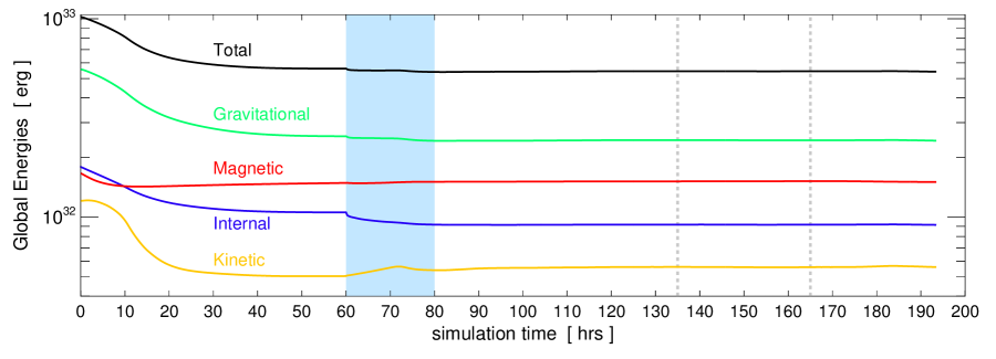
Figure 6: Global energy evolution: total (black), gravitational (green), magnetic (red), internal (blue), and kinetic (yellow). The solar wind relaxation phase duration is from $0\leq t\leq 60$ h. The shearing phase is $60\leq t\leq 80$ h (shaded light blue). The vertical dashed lines indicate the start of the synthetic running difference movie (Figure 11) at $t=135$ h and when the leading edge of the CME enters the COR2A field of view ($r=2.5$R_⊙) at $t=165$ h.

Figure 6 plots the full energy evolution of the MHD system over the 194 h of simulation time. We have plotted the total (black), gravitational (green), magnetic (red), internal (blue), and kinetic (orange) energies. For $t\leq 60$ h the system relaxes until the isothermal solar wind solution and the initial PFSS magnetic configuration equilibrate. The values at the end of the relaxation phase are $E_{\rm tot}=5.611\times 10^{32}$ ergs, $E_{\rm grv}=2.559\times 10^{32}$ ergs, $E_{\rm mag}=1.489\times 10^{32}$ ergs, $E_{\rm int}=1.058\times 10^{32}$ ergs, and $E_{\rm kin}=5.054\times 10^{31}$ ergs.

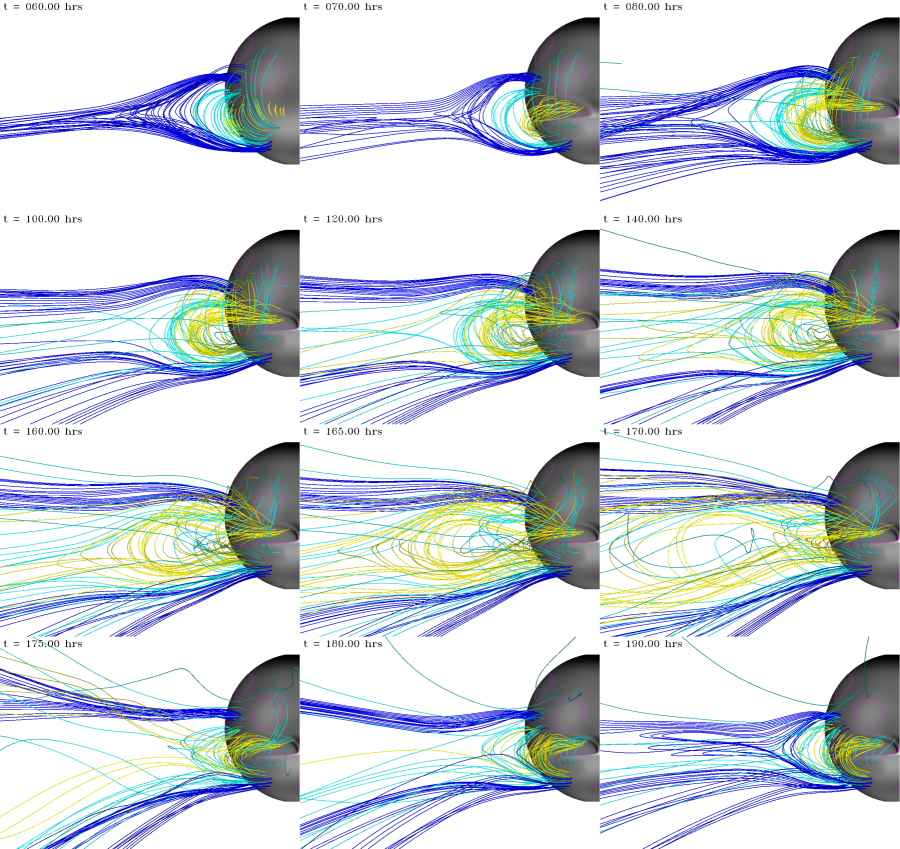
Figure 7: Visualization of the magnetic field evolution. The magnetic field lines are colored by their connectivity at $t=60$ h: Yellow field lines are traced from points within the shear channel and become the highly sheared core flux that eventually erupts; light blue field lines show the restraining closed flux of the helmet streamer outside of the shear channel; dark blue field lines show the boundary of the helmet streamer and adjacent open fields. For $t\geq 80$ h, all of the field lines are traced from static foot points showing the topological evolution of the stealth streamer blowout CME. An animation of this figure is available as supporting information of the article.

Figure 7 shows representative magnetic field lines during the simulation. The magnetic field lines are colored by their magnetic topology at $t=60$ h. The dark blue field lines show the largest-scale streamer field lines and open fields just outside the helmet streamer boundary. The light blue field lines show the overlying closed streamer flux that originates outside of the shear channel. The yellow field lines are traced from positions within the shear channel and show the energized arcade flux.

The top row in Figure 7 shows the shearing of the bipolar arcade for $t\in[60,80]$ h. The magnetic flux distribution on the lower radial boundary remains fixed for $t\geq 80$ h. The second row shows the slow arcade expansion during $100{\;\rm h}\leq t\leq 140{\;\rm h}$. As the arcade expands, the light blue flux gradually opens into the solar wind. As this overlying flux opens up, the restraining tension force decreases, allowing the sheared flux core to expand further in a positive-feedback loop reminiscent of the magnetic breakout (Antiochos et al., 1999; Lynch et al., 2008) or tether-cutting (Moore et al., 2001) CME initiation mechanisms. Rather than reconnecting at an overlying breakout current sheet and being transferred to adjacent arcades as in the classic breakout scenario, here the restraining flux gradually expands into solar wind to become open. The sheared arcade expansion forms a radial current sheet that elongates, thins and eventually facilitates magnetic reconnection in the standard CSHKP scenario. The third row in Figure 7 shows the onset of eruptive flare reconnection for $t\gtrsim 160$ h. This magnetic field reconfiguration creates a flux rope-like structure during the eruption process. The bottom row in Figure 7 shows the posteruption reconnection that reforms the helmet streamer beneath the CME for $t\gtrsim 175$ h.

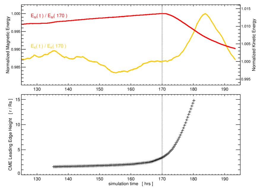
Figure 8: (top) Normalized global magnetic and kinetic energies during the slow stealth CME eruption. We normalize by the values at $t=170$ h (dashed vertical line) where the eruptive flare reconnection is most visible in Figure 7. The stealth CME eruption corresponds to only a 1.0% drop in total magnetic energy ($1.49\times 10^{30}$ ergs) and a 1.4% increase in total kinetic energy ($7.62\times 10^{29}$ ergs). (bottom) Height-time evolution of the sheared arcade expansion and slow CME eruption.

Figure 8 (top) plots the global magnetic and kinetic energies during the eruption normalized to their respective values at $t=170$ h. The shape of the energy curves are exactly as expected from our previous simulations of CME events: the magnetic energy decreases and the kinetic energy increases as the erupting fields are removed from the low corona. We note that for $t\gtrsim 187$ h, some portion of both the global magnetic and kinetic energy decrease is due to the CME passing through the simulation outer boundary. Figure 8 (bottom) shows the height-time evolution of the leading edge of the expanding arcade and CME derived from the analysis discussed in section 3.3.3. The height-time profile shows the smooth transition for $165\lesssim t\lesssim 175$ h from the linear rising phase of the sheared arcade to the full CME eruption and its associated increase in the global kinetic energy. This transition corresponds to the onset and development of eruptive flare reconnection and its rapid reconfiguration of the magnetic field connectivity (as seen in the $t=160$, $165$, and $170$ h panels in Figure 7). The relative timing of the onset of flare reconnection and the resulting acceleration during the transition from expanding arcade to erupting flux rope suggests that our eruption mechanism is that of a resistive instability in the radial current sheet.

There are other ideal MHD instabilities that can initiate CME eruptions such as loss-of-equilibrium (Forbes et al., 2006), in which the system suffers a catastrophic change in the equilibrium states available to it, and the torus instability (Kliem and Török, 2006), in which an equilibrium flux rope becomes ideally unstable to outward displacements into a region of substantially weaker field. In either of these ideal instability cases, we would expect to observe the onset of outward motion before flare reconnection sets in below the rising sheared arcade, whereas we observe the outward acceleration only after the flare reconnection sets in. Additionally, ideal MHD instabilities require a net current, in other words, twist, which is either obtained by the presence of a preeruption twisted flux rope (e.g., Török and Kliem, 2005; Kliem and Török, 2006; Fan, 2010) or created via flux cancelation (Linker et al., 2003; Amari et al., 2010; Aulanier, 2014). There has never been an “ideal eruption” of a sheared arcade, nor can there be, irrespective of how high the sheared flux expands to. The key point is that the flare reconnection allows the system to evolve to a much lower energy state than it could ever get to by ideal expansion.

Therefore, despite the slow, gradual character of our stealth CME eruption, the main acceleration mechanism is the same as in the fast 2.5D magnetic breakout CME discussed by Karpen et al. (2012): the onset of flare reconnection forms and accelerates the CME flux rope. The key property of the evolution that is responsible for eruption is that the outward expansion results in the formation of a large, vertical current sheet deep inside the closed field system. As concluded by Karpen et al. (2012), once reconnection sets in at this flare current sheet, the system must erupt with the ejection of a large flux rope. This conclusion appears to apply to our stealth CME as well, even though the system is fully 3-D. Without reconnection, the sheared flux could open (“erupt”) via ideal expansion but the large vertical current sheet would extend down very close to the surface. This open state has much greater magnetic energy than the potential state. The eruptive flare reconnection allows the system to take the difference between the energy of this open state and the potential state and put it into accelerating the CME plasma and opening up a small fraction of the low-lying flux. It is unclear whether smooth flux opening by ideal expansion would be classified as a CME by an observer.

The flare reconnection is essential to the CME eruption in that the CME’s magnetic structure is a consequence of this reconnection. Specifically, (1) the eruptive flare reconnection creates a flux rope structure from the expanding arcade, and (2) this reconnection enables the removal of a significant amount of sheared (and due to reconnection, increasingly twisted) flux from the closed field corona as a coherent structure. Without the flare reconnection, the opening flux will be substantially less “coherently structured” and will not exhibit the flux rope-like cross-sectional morphology in coronagraph images. At the same time, we show that for this stealth CME, the acceleration during an eruption with relatively weak flare reconnection can be small. There is some acceleration in our simulation, the global kinetic energy does increase from 170–184 h, but it is not very substantial. Consequently, the resulting CME speeds are comparable to the background solar wind.

There is a hierarchy of energetics associated with reconnection-driven eruption of closed flux. Large flares that generate fast CMEs originate in very low lying fields above polarity inversion lines of active regions. Streamer blobs are generated at the edges of the closed flux regions, near the open-closed field interface, i.e. relatively weak fields at the boundaries of coronal holes and/or even weaker fields in the extended corona. Stealth CMEs, and likely all slow streamer blowout CMEs, are essentially an intermediate case between these two extremes. They originate at intermediate heights in the closed field regions and thus have a much larger spatial extent than streamer blobs but are much less energetic than fast CMEs. Magnetic reconnection is required for all of these structures to “erupt” (be released) into the open field with a coherent flux rope-like magnetic structure.

3.2.2 Eruptive Flare–CME Energy Budget

Our CME simulation can be considered a “stealth” event because the magnitude of both the magnetic energy decrease and the CME’s kinetic energy increase are relatively small. From Figure 8, the global magnetic energy released over the course of the eruption is $\sim$1.0% ($\Delta E_{M}=1.49\times 10^{30}$ ergs) and the peak of the global kinetic energy is $\sim$1.4% ($\Delta E_{K}=7.62\times 10^{29}$ ergs) compared to the preeruption values. The temporal and spatial scales over which the released magnetic energy is deposited are also extremely important in characterizing the eruptive flare/CME event dynamics.

An upper limit estimate of the Poynting flux, $\tilde{S}$, into the stealth CME flare current sheet can be obtained via

$$\frac{\partial E_{M}}{\partial t}=\oint\boldsymbol{S}\cdot{d\boldsymbol{A}}\ \Longrightarrow\ \frac{\Delta E_{M}}{\Delta t}\sim\tilde{S}\Delta A.$$ (9)

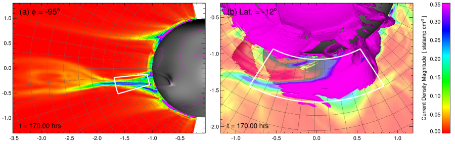
Figure 9: Current density magnitude $|J|$ of the eruptive flare current sheet at $t=170$ h. (a) The $r$-$\theta$ plane at $\phi=-95^{\circ}$. (b) Transparent $r$-$\phi$ plane at latitude $-12^{\circ}$ with the magenta isosurface at $|J|=0.35$ statamp cm^-2. The white spherical wedge regions indicate the radial and azimuthal areas used in the equation (10) estimate of the energy density flux available to generate plasma heating and flare emission signatures.

Figure 9 shows two viewpoints of the current density magnitude $|J|$ in the flare current sheet at $t=170$ h: (a) in the $r$-$\theta$ plane at $\phi=-95^{\circ}$; and (b) in the (transparent) $r$-$\phi$ plane at latitude $-12^{\circ}$. Figure 9b also plots the 3-D isosurface of $|J|=0.35$ statamp cm^-2. An estimate of the $r$-$\phi$ planar wedge area associated with the stealth CME current sheet is calculated from $r\in[1.1R_{\odot},1.7R_{\odot}]$ and $\phi\in[-65^{\circ},-125^{\circ}]$ at latitude $\lambda=-12^{\circ}$. This gives an area of $\Delta A=4.21\times 10^{21}$ cm². Taking the duration of the magnetic energy drop as 24 h from Figure 8 ($\Delta t=8.64\times 10^{4}$ s), we get

$$\tilde{S}=\frac{(1.49\times 10^{30}{\;\rm erg})}{(4.21\times 10^{21}{\;\rm cm}^{2})(8.64\times 10^{4}{\;\rm s})}=4.10\times 10^{3}{\;\rm erg\;cm^{-2}\;s^{-1}}.$$ (10)

This estimate of the energy flux into the stealth CME’s large-scale current sheet over the course of the eruption is about 2 orders of magnitude below the average energy flux necessary to heat the ambient solar corona and accelerate the solar wind ($\sim$$10^{5-6}$ erg cm^-2 s^-1) (e.g., Withbroe and Noyes, 1977; Fisk et al., 1999; Cranmer and van Ballegooijen, 2010). Therefore, it is not at all surprising that the 1–2 June 2008 stealth CME event did not produce any significant, or observable, flare emission and posteruption brightening (heating) in the low corona.

3.3 Comparison to Observations

3.3.1 Current Sheet X Point Structure

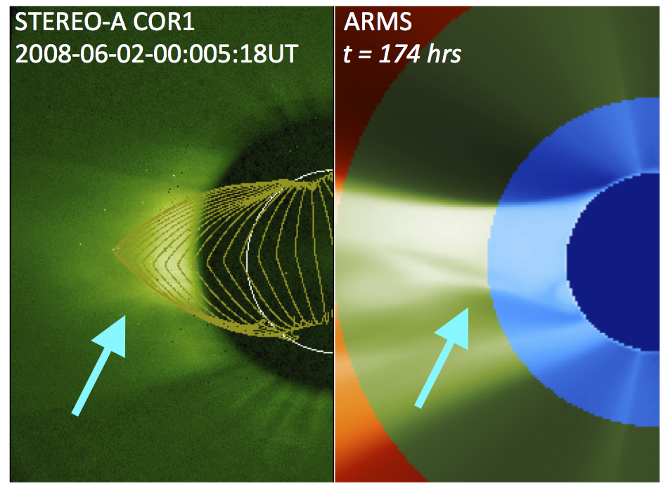
Figure 10: (left) STA-COR1 observation with representative PFSS field lines overplotted showing the faint white-light signature of the eruption X point (adapted from Lynch et al., 2010). (right) Synthetic white-light ratio image at $t=174$ h from $\phi_{\rm STA}$ perspective showing the stealth CME simulation X point structure.

Current sheets trailing CME eruptions have been observed in white-light coronagraph observations (e.g., Webb et al., 2003; Lin et al., 2005; Poletto et al., 2008; Patsourakos and Vourlidas, 2011; Song et al., 2012) as well as EUV imaging and spectroscopy and X-rays (e.g., Bemporad et al., 2006; Savage et al., 2010; Liu et al., 2010; Liu, 2013; Landi et al., 2012; Ciaravella et al., 2013; Susino et al., 2013). Given the upper limit estimate of the magnetic energy flux available for bulk plasma heating and particle acceleration associated with our stealth CME current sheet, we do not expect any of the typical coronal EUV or X-ray emission signatures associated with high-energy eruptive flare events. Figure 10 compares the faint white-light observation of the CME-trailing eruptive flare current sheet and X point morphology in the STEREO-A COR1 coronagraph (Figure 10, left) with the corresponding synthetic white-light emission calculated from the MHD simulation (Figure 10, right). The intensity enhancement suggestive of the X point morphology is quite high in the corona, $\sim$1.5$R_{\odot}$. There is good correspondence between the white-light intensity structures observed by COR1A and that generated from the simulation data.

3.3.2 Three-Part CME Structure

The three-part morphology of CMEs in white-light coronagraph observations is one of the best proxy measures of the plasma and magnetic field structure of CMEs (e.g., Illing and Hundhausen, 1985; Dere et al., 1999; Wood et al., 1999; Cremades and Bothmer, 2004; Rouillard, 2011; Vourlidas et al., 2013). Here we present a favorable comparison between the observed large-scale white-light morphology of the 1–2 June 2008 CME and the synthetic white-light structure derived from the simulated flux rope CME density distribution.

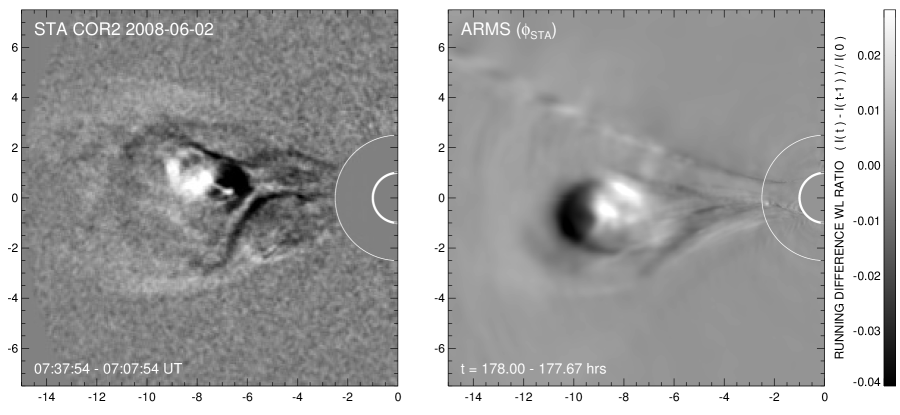
Figure 11: (left) STA-COR2 running difference image at 07:37UT on 2 June 2008 showing the three-part white-light structure of the flux rope CME. (right) Running difference image of synthetic white-light ratio images at $t=178$ h showing the three-part structure in the simulated CME. An animation of the simulated running difference evolution is available as supporting information of the article.

Figure 11 plots the STA COR2 running difference image showing the circular cross section of the stealth CME at $\sim$10$R_{\odot}$ (Figure 11, left) and the corresponding simulation results (Figure 11, right). The simulation running difference images are calculated from the synthetic total white-light brightness ratio images as $(I(t)-I(t-1))/I(0)$ using simulation output files generated every 20 min of simulation time. The opening angle of the eruptive structure and the relative size of the circular cross section are in excellent qualitative agreement. Our simulation also produces the bright core density enhancement at the center of the flux rope. This is an improvement over our earlier 2.5-D (Lynch et al., 2004) and 3-D (Vourlidas et al., 2013) results. The solar wind boundary conditions used here allow additional mass to accumulate in the closed field region before being transferred by the flare reconnection outflow into the erupting flux rope structure. On the other hand, our simulation shows the running difference signature of a dark cavity ahead of the bright core, whereas in the STA COR2 observations the running difference signature of the cavity region is much less pronounced. This seems to be due to the simulated flux rope cavity being more depleted relative to the ambient streamer density than the observed streamer blowout CME. In fact, many CMEs generally do show the well-known three-part structure of a bright front followed by a dark cavity and then a bright core, but the structure appears to be reversed in this stealth event. This is likely due to the long buildup phase of this CME, which allowed for substantial mass transfer from the corona into the ejecting plasmoid during its development. Our shearing phase, however, is approximately 20 times faster than the Sun’s equivalent differential rotation energization timescale of $\sim$15 days. Furthermore, our use of an isothermal plasma energy equation is likely to underestimate the effects of plasma heating and chromospheric evaporation.

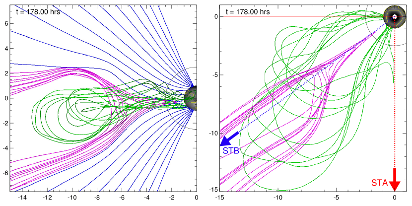
Figure 12: (left) Representative magnetic field lines of the stealth CME eruption for the ARMS $\phi_{\rm STA}$ field of view in Figure 11 . Shown are the sheared arcade field lines that become the flux rope CME (green), the reconnecting open fields behind the eruption (magenta), and the background open field lines (blue). (right) The same green and magenta field lines from the North solar pole. The longitudinal positions of the STA and STB spacecraft in the simulation are shown with the red and blue arrows, the STA COR2 plane of the sky as the solid red line.

Following Vourlidas et al. (2013), here we analyze the simulation’s magnetic flux rope structure and topology from the synthetic STA viewpoint in Figure 11. Figure 12 (left) plots representative magnetic field lines from the simulation at $t=178$ h colored by their magnetic connectivity. The erupting flux rope field lines are shown in green, the newly reconnected field lines behind the eruption are shown in magenta, and the background open field lines are shown in blue. The faint, running difference leading edge enhancement occurs just ahead of the approximately circular cross section of the green flux rope field lines. The green field line cross section corresponds to the dark running difference cavity. The running difference bright core enhancement is located at the back of the flux rope at the interface of the green and magenta field lines, suggesting that it originates in the large-scale flare reconnection outflow. In fact, the running-difference Y-shaped feature behind the eruption is now easily related to the reconnecting fields at the eruptive flare current sheet.

Figure 12 (right) plots the green and magenta CME lines from the top-down perspective looking at the north solar pole. The heliospheric longitude position of the STA and STB spacecraft relative to the simulation data are shown as the red and blue arrows, respectively. There are two important features. First, the radial trajectory of the stealth CME is more directed towards STB rather than lying in the STA plane of the sky. Second, the relatively compact circular cross section of green flux rope field lines seen in Figure 12 (left) is a projection effect—the synthetic COR2A plane of the sky is shown as the horizontal red line at $y=0$. The core flux rope field lines have a greater radial extent in the portion of the flux rope between the STB and STA position angles. In addition, the 3-D stealth CME structure has a significant large-scale writhe component in the magnetic field, which can be difficult to distinguish from twisted flux rope fields in in situ data (e.g., Jacobs et al., 2009; Al-Haddad et al., 2011). Our stealth CME magnetic field structure in the coronagraph field of view is that of a twisted flux rope, just not a highly twisted flux rope. The amount of poloidal twist flux contained in the erupting magnetic structure should be directly proportional to the amount of flare reconnection during the eruption, especially for sheared arcade preeruption states (e.g., Longcope et al., 2007; Kazachenko et al., 2012). Therefore, it is completely reasonable that our slow CME having undergone relatively weak flare reconnection ends up less twisted than more energetic CMEs with greater reconnection flux during their eruptive flares.

3.3.3 Height-Time and CME Speed Profile

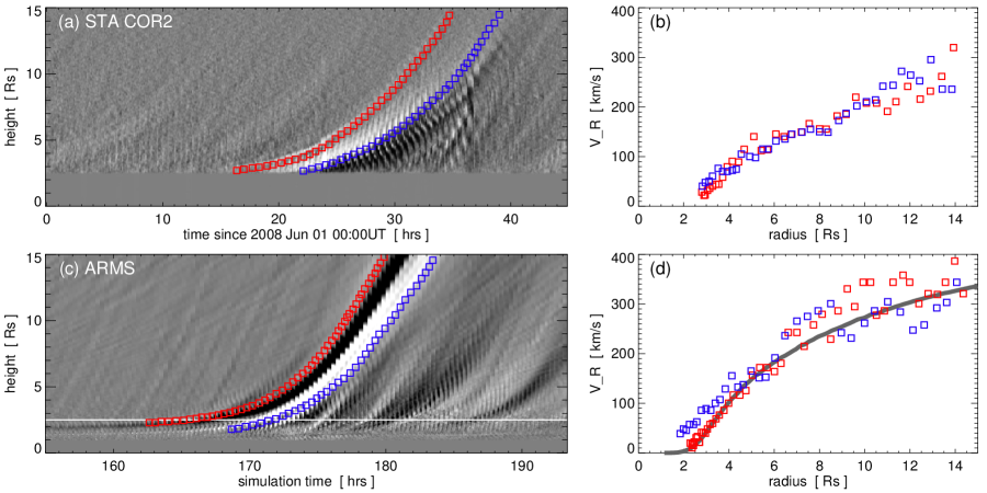
Figure 13: (a) STA-COR2 running difference “J-map” with height-time points for the CME leading edge (red squares) and core region (blue squares) overplotted. (b) The apparent radial velocity calculated from the height-time tracks as a function of $r$. (c) The simulated height-time “J-map.” (d) The simulated CME velocity profile. The black line is the ambient solar wind profile at the equator from Figure 3.

Ma et al. (2010) examined the STEREO COR1 and COR2 signatures of slow CME events both with and without low coronal signatures during solar minimum (January–August 2009) and found that approximately one third of their CMEs could be considered stealth events. These events were consistently at the lower end of the slow CME velocity profile distribution ($V_{r}<300$ km s^-1 by $\sim$15$R_{\odot}$). Vourlidas et al. (2000) calculated the velocity and acceleration profiles, as well as the kinetic energies, of 11 CMEs with flux rope morphologies in LASCO observations during the previous solar miniumum (1997). Their five slowest events ($V_{r}\leq 350$ km s^-1 by $\sim$20$R_{\odot}$) corresponded to kinetic energy estimates in the range of $3-5\times 10^{29}$ ergs, in good agreement with our simulation results. Figure 13 compares the height-time and velocity profiles for the 1–2 June 2008 CME observations (Figures 13a and 13b) and our simulation (Figures 13c and 13d). Figures 13a and 13c plot the height-time “J-maps” (Sheeley et al., 1997) constructed from the running-differenced STA COR2 data and our synthetic white-light images. The red squares track the cavity leading edge and the blue squares track the trailing edge of the CME core enhancement of the eruption; these points are used to calculate the apparent $V_{r}(r)$ profiles plotted in Figures 13b and 13d. In Figure 13d we also plot the equatorial background solar wind profile from Figure 3 as the black line. In both the observations and simulation, the CME core velocities are slightly higher than the leading edge velocities for $r\lesssim 4R_{\odot}$, indicative of the additional acceleration the core material experiences from originating in the flare reconnection jets. For $r\gtrsim 4R_{\odot}$, this separation has disappeared, implying that, at least for $r\gtrsim 4R_{\odot}$, our stealth CME flux rope is now advecting passively with the background flow.

3.3.4 Synthetic In Situ Time Series at 15$R_{\odot}$

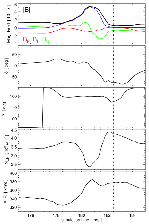
Figure 14: Synthetic in situ time series of field and plasma properties at $\boldsymbol{r}=(15R_{\odot},\>0^{\circ},\>\phi_{\rm STB})$. From top to bottom, $B$ magnitude (black) and RTN components ($B_{R}$ red; $B_{T}$ blue; $B_{N}$ green), magnetic field direction ($\delta$, $\lambda$), number density $N_{p}$, and radial velocity $V_{r}$. Vertical dotted lines denote period of coherent, ICME flux rope rotation.

For the time period $t\in\left[175,185\right]$ h we have increased the temporal cadence of the simulation output files to once per 5 min to construct the synthetic time series of plasma and field properties seen by a stationary observer at $\boldsymbol{r}=(15R_{\odot},\>0^{\circ},\>\phi_{\rm STB})$. Figure 14 shows, from top to bottom, magnetic field magnitude (black) and components in RTN coordinates ($B_{R}=B_{r}$, red; $B_{T}=B_{\phi}$, blue; $B_{N}=-B_{\theta}$, green), magnetic field direction (in RTN latitude $\delta$ and RTN longitude $\lambda$), plasma number density $N_{p}$, and radial plasma velocity $V_{r}$. The synthetic in situ time series shows many of the classic characteristics of flux rope ICMEs, often referred to as magnetic clouds, including the enhanced magnetic field magnitude, a smooth, coherent rotation in the field direction, and a lower density region corresponding to a lower in situ temperature (Bothmer and Schwenn, 1998; Lynch et al., 2005; Li et al., 2011, 2014).

4 Discussion

4.1 Implications for CME Initiation and Large-Scale Coronal Evolution

Recent observations of coronal mass ejections that lack typical low coronal signatures, such as EUV or X-ray flaring and ribbons, have led to them being characterized as a new and mysterious type of “stealth CME.” However, every individual component of our MHD simulation—the low-order PFSS field representation (Altschuler and Newkirk, 1969; Schatten et al., 1969; Wang and Sheeley, 1992), the isothermal solar wind model (Parker, 1958), and sheared arcade model for CMEs (Forbes and Priest, 1982, 1983; Mikic et al., 1988; Mikić and Linker, 1994; Linker and Mikić, 1995; Antiochos et al., 1999)—is 30 to 60 years old. Yet we have shown that these components, when combined with modern computational techniques, lead to a 3-D eruption scenario that accounts for a majority of the qualitative features of the 1–2 June 2008 stealth CME.

The physical processes associated with the gradual shearing energization and the resulting arcade expansion that lead to large-scale magnetic reconfiguration with relatively weak (low energy) eruptive flare reconnection are about as fundamental and generic as possible—and have been observed for decades. Therefore, not only have we demonstrated a successful model for stealth CME eruptions but we also argue that essentially all slow streamer blowout CMEs are likely to be some variation of this scenario.

Lynch et al. (2010) presented a back of the envelope calculation of the occurrence rate and total number of slow streamer blowout CMEs generated by the coronal evolution in response to large-scale, photospheric processes such as differential rotation. We obtained an estimate of approximately eight CMEs per month over the whole streamer belt; this was approximately half the rate in CDAW LASCO CME catalog for slow CMEs $>$30^∘ in angular width during the 2008–2009 solar minimum. The starting point of this estimate was generating the required magnetic fluxes from the initial PFSS helmet streamer field to match the observed in situ flux content of the 6–7 June 2008 ICME magnetic cloud flux rope at STEREO-B. Here our MHD simulation results have confirmed the basic assumption underlying the Lynch et al. (2010) discussion: a large-scale shear (equivalent to $\sim$2 weeks of differential rotation over 40^∘ latitude) applied to the bipolar helmet streamer could produce a slow, flux rope-like streamer blowout eruption, such as observed by STEREO-A on 1–2 June 2008. Our simulation results are consistent with the Hudson and Li (2010) conclusion that “the observation that CMEs continue into solar minimum whereas flares do not, or else become less important, suggests the existence of a CME mechanism basically independent of the activity level.”

The ICME flux rope orientation over the solar cycle (e.g., Zhao and Hoeksema, 1996; Bothmer and Rust, 1997; Bothmer and Schwenn, 1998; Mulligan et al., 1998; Li et al., 2011, 2014) provides additional evidence that global-scale photospheric evolutionary processes, modulated by the magnetic field structure and evolution of the corona, are the underlying cause for a significant fraction of CME activity. Lynch et al. (2005) examined the flux and helicity content of magnetic cloud flux rope ICMEs from 1995 to 2003. We showed the net cumulative helicity of 108 “slow events” ($V_{\rm ICME}<500$ km s^-1) essentially averaged to zero over the 8 year period. A net cumulative helicity of zero is exactly as expected if the ICME helicity originates from a large-scale velocity pattern that is symmetric with respect to the equator acting on a large-scale, antisymmetric magnetic field, i.e., differential rotation acting on the global dipole magnetic field (DeVore, 2000).

We conclude from this discussion and from the results above that, in many ways, stealth CMEs bridge the gap between the standard events driven by filament channel eruption and the small-scale plasmoids that are observed to be continuously emitted from streamer tops (Viall and Vourlidas, 2015). According to the S-Web model, these plasmoids are due to the reconnection dynamics of coronal hole boundaries driven by the photospherc convective motions (Antiochos et al., 2011). If so, then fast CMEs, stealth CMEs and streamer plasmoids may well constitute a continuum of manifestations of a single process: the ejection of magnetic stress into the heliosphere via reconnection. For fast CMEs the magnetic stress builds up on the lowest-lying flux near polarity inversion lines. For streamer top plasmoids the stress is injected on the highest-lying flux near the boundary of the closed field system. In stealth CMEs the stress is injected at intermediate heights by the large-scale differential rotation. In all cases the stress appears to be released by the formation and ejection of a reconnection plasmoid similar to the breakout CME simulations of Karpen et al. (2012). If this “unified” scenario is correct, it could greatly simplify our understanding and modeling of coronal evolution. Detailed studies of stealth CMEs, which are relatively easy to observe accurately due to their large spatial and temporal scales, may well provide key insights into phenomena at smaller and/or much faster scales.

4.2 Implications for Space Weather Forecasting

The STEREO mission space weather capabilities and NOAA Space Weather Prediction Center forecasting requirements are discussed by Biesecker et al. (2008). Typical on-disk signatures such as soft X-ray sigmoid/arcade emission, filament eruptions in H$\alpha$ or EUV, UV flare ribbon emission, and/or large-scale coronal dimmings, followed by halo or partial-halo CMEs, act as a 2–5 day precursor warning for potential geomagnetic storms from Earth-impacting events. Stealth CMEs are a problematic type of event to effectively forecast due to the lack of on-disk signatures and their halo signatures being difficult to observe in coronagraph data. For example, Webb et al. (2000) analyzed a faint Earth-directed halo CME that caused significant geomagnetic activity.

The 1–2 June 2008 stealth CME produced an extremely faint halo CME signature in the STB COR2 running difference images only visible for a few frames (Robbrecht et al., 2009). However, as we have shown here and in Lynch et al. (2010), STA was able to image a well-resolved, edge-on flux rope CME in COR2 and track its propagation through HI1 and HI2 all the way to its impact with STB at 1 AU. This fortuitous observing geometry was due to the $\approx$55^∘ separation between the STEREO spacecraft. Our simulation’s synthetic running difference images from the STB viewing perspective do contain halo CME-like signatures but only at the level of the running difference fluctuations caused by the ambient solar wind outflow. In other words, it would be almost impossible to identify the simulated CME from this viewpoint alone.

The L5 Lagrange point at 1 AU, located 60^∘ from the Sun-Earth line, is ideally suited for identifying and observing such Earth-directed stealth CME events. Indeed, the prospect of an L5 space weather mission for operational forecasting has generated considerable community and agency support (e.g., Gopalswamy et al., 2011; Howard et al., 2012; Lavraud et al., 2014; Trichas et al., 2015). Our simulation results, the eruption of a large-scale coherent flux rope CME towards STB with almost no discernible halo or partial-halo CME signatures, highlights the importance of supplementing the traditional L1 viewpoint for space weather forecasting.

5 Summary and Conclusions

We have presented a numerical simulation of the 1–2 June 2008 stealth CME and shown that all of the qualitative large-scale properties of the slow streamer blowout CME are reproduced by our calculation.

1. The 3-D preeruption global coronal structure in multiviewpoint synthetic white-light coronagraph images captures the overall shape and location of the helmet streamer and pseudostreamer structures in CR2070.

2. We energized the bipolar helmet streamer over the source region estimate by Robbrecht et al. (2009) via large-scale shearing flows with respect to the streamer belt polarity inversion line, obtaining a total foot point displacement equivalent to $\sim$2 weeks of differential rotation.

3. The sheared helmet streamer arcade expands slowly over the next several days, gradually opening more restraining overlying flux into the solar wind. The gradual opening of the helmet streamer flux facilitates continued arcade expansion, which opens more closed flux in a positive feedback loop similar to the runaway expansion in the Antiochos et al. (1999) breakout model for CME initiation. However, unlike the breakout model, in which the restraining flux is rapidly transferred through magnetic reconnection, the gradual expansion-driven opening of helmet streamer flux into the solar wind is a relatively slow disruption of pressure balance.

4. Given the low magnetic field strengths associated with the quiet-Sun flux distribution and the spatial scale of the helmet streamer system, the stored magnetic energy released during our stealth CME eruptive flare reconnection is $\sim$10³⁰ erg over a time of $\gtrsim$20 h. Our estimate of the available magnetic energy flux for observable flare heating and emission during the eruption is 2 orders of magnitude below the energy flux required to heat the ambient background corona.

5. Our simulation produces the observed white-light signatures of the X point flare current sheet in the STA COR1 field of view, the three-part structure of flux rope CMEs in synthetic running difference images, and the height-time and velocity profiles of the CME propagation through $\sim$15$R_{\odot}$ in excellent agreement with the STA COR2 observations. Our velocity profile implies that the stealth CME structure is passively advected with the background solar wind.

6. Our results support the Howard and Harrison (2013) argument that stealth CMEs are not fundamentally different from most slow streamer blowout CMEs; they simply represent the lowest-energy range of the (slow) CME distribution.

We have discussed the implications of our stealth CME simulation results for sheared arcade models of CME initiation, their relationship to the global evolution of the large-scale corona, and for future research on the space weather consequences of stealth CMEs.

References

- Al-Haddad et al. (2011) Al-Haddad, N., I. I. Roussev, C. Möstl, C. Jacobs, N. Lugaz, S. Poedts, and C. J. Farrugia (2011), On the Internal Structure of the Magnetic Field in Magnetic Clouds and Interplanetary Coronal Mass Ejections: Writhe versus Twist, ApJ 738, L18, 10.1088/2041-8205/738/2/L18.
- Allred and MacNeice (2015) Allred, J. C., and P. J. MacNeice (2015), An MHD code for the study of magnetic structures in the solar wind, Computational Science and Discovery, 8(1), 015002, 10.1088/1749-4680/8/1/015002.
- Altschuler and Newkirk (1969) Altschuler, M. D., and G. Newkirk (1969), Magnetic Fields and the Structure of the Solar Corona. I: Methods of Calculating Coronal Fields, Solat Phys., 9, 131–149, 10.1007/BF00145734.
- Alzate and Morgan (2016) Alzate, N., and H. Morgan (2016), Low-Coronal Sources of Stealth CMEs, in AAS/Solar Physics Division Meeting, vol. 47, #102.04.
- Amari et al. (2010) Amari, T., J.-J. Aly, Z. Mikić, J. Linker (2010), Coronal Mass Ejection Initiation: On the Nature of the Flux Cancellation Model, ApJ, 717, L26, 10.1088/2041-8205/717/1/L26.
- Antiochos et al. (1999) Antiochos, S. K., C. R. DeVore, and J. A. Klimchuk (1999), A Model for Solar Coronal Mass Ejections, ApJ 510, 485–493, 10.1086/306563.
- Antiochos et al. (2011) Antiochos, S. K., Z. Mikić, V. S. Titov, R. Lionello, J. A. Linker (2011), A Model for the Sources of the Slow Solar Wind, ApJ 731, 112, 10.1088/0004-637X/731/2/112.
- Aulanier (2014) Aulanier, G. (2014), The physical mechanisms that initiate and drive solar eruptions, in Nature of Prominences and their Role in Space Weather, IAU Symposium, vol. 300, edited by B. Schmieder, J.-M. Malherbe, and S. T. Wu, pp. 184–196, 10.1017/S1743921313010958.
- Bemporad et al. (2006) Bemporad, A., G. Poletto, S. T. Suess, Y.-K. Ko, N. A. Schwadron, H. A. Elliott, and J. C. Raymond (2006), Current Sheet Evolution in the Aftermath of a CME Event, ApJ 638, 1110–1128, 10.1086/497529.
- Biesecker et al. (2008) Biesecker, D. A., D. F. Webb, and O. C. St. Cyr (2008), STEREO Space Weather and the Space Weather Beacon, Space Sci. Rev., 136, 45–65, 10.1007/s11214-007-9165-7.
- Billings (1966) Billings, D. E. (1966), A GUIDE TO THE SOLAR CORONA, New York: Academic Press.
- Bisi et al. (2010) Bisi, M. M., B. V. Jackson, P. P. Hick, A. Buffington, J. M. Clover, M. Tokumaru, and K. Fujiki (2010), Three-dimensional Reconstructions and Mass Determination of the 2008 June 2 LASCO Coronal Mass Ejection Using STELab Interplanetary Scintillation Observations, ApJ 715, L104–L108, 10.1088/2041-8205/715/2/L104.
- Bothmer and Rust (1997) Bothmer, V., and D. M. Rust (1997), The field configuration of magnetic clouds and the solar cycle, Washington DC American Geophysical Union Geophysical Monograph Series, 99, 139–146, 10.1029/GM099p0139.
- Bothmer and Schwenn (1998) Bothmer, V., and R. Schwenn (1998), The structure and origin of magnetic clouds in the solar wind, Annales Geophysicae, 16, 1–24, 10.1007/s00585-997-0001-x.
- Carmichael (1964) Carmichael, H. (1964), A Process for Flares, NASA Special Publication, 50, 451.
- Cheung and DeRosa (2012) Cheung, M. C. M., and M. L. DeRosa (2012), A Method for Data-driven Simulations of Evolving Solar Active Regions, ApJ 757, 147, 10.1088/0004-637X/757/2/147.
- Ciaravella et al. (2013) Ciaravella, A., D. F. Webb, S. Giordano, and J. C. Raymond (2013), Bright Ray-like Features in the Aftermath of Coronal Mass Ejections: White Light versus Ultraviolet Spectra, ApJ 766, 65, 10.1088/0004-637X/766/1/65.
- Cranmer and van Ballegooijen (2010) Cranmer, S. R., and A. A. van Ballegooijen (2010), Can the Solar Wind be Driven by Magnetic Reconnection in the Sun’s Magnetic Carpet?, ApJ 720, 824–847, 10.1088/0004-637X/720/1/824.
- Cremades and Bothmer (2004) Cremades, H., and V. Bothmer (2004), On the three-dimensional configuration of coronal mass ejections, A&A 422, 307–322, 10.1051/0004-6361:20035776.
- Dere et al. (1999) Dere, K. P., G. E. Brueckner, R. A. Howard, D. J. Michels, and J. P. Delaboudiniere (1999), LASCO and EIT Observations of Helical Structure in Coronal Mass Ejections, ApJ 516, 465–474, 10.1086/307101.
- DeVore (1991) DeVore, C. R. (1991), Flux-corrected transport techniques for multidimensional compressible magnetohydrodynamics, Journal of Computational Physics, 92, 142–160, 10.1016/0021-9991(91)90295-V.
- DeVore (2000) DeVore, C. R. (2000), Magnetic Helicity Generation by Solar Differential Rotation, ApJ 539, 944–953, 10.1086/309274.
- DeVore and Antiochos (2000) DeVore, C. R., and S. K. Antiochos (2000), Dynamical Formation and Stability of Helical Prominence Magnetic Fields, ApJ 539, 954–963, 10.1086/309275.
- DeVore and Antiochos (2008) DeVore, C. R., and S. K. Antiochos (2008), Homologous Confined Filament Eruptions via Magnetic Breakout, ApJ 680, 740–756, 10.1086/588011.
- D’Huys et al. (2014) D’Huys, E., D. B. Seaton, S. Poedts, and D. Berghmans (2014), Observational Characteristics of Coronal Mass Ejections without Low-coronal Signatures, ApJ 795, 49, 10.1088/0004-637X/795/1/49.
- Fan (2010) Fan, Y. (2010), On the Eruption of Coronal Flux Ropes, ApJ, 719, 728–736, 10.1088/0004-637X/719/1/728.
- Fisk et al. (1999) Fisk, L. A., N. A. Schwadron, and T. H. Zurbuchen (1999), Acceleration of the fast solar wind by the emergence of new magnetic flux, J. Geophys. Res. 104, 19,765–19,772, 10.1029/1999JA900256.
- Forbes and Priest (1982) Forbes, T. G., and E. R. Priest (1982), Numerical study of line-tied magnetic reconnection, Solar Phys., 81, 303–324, 10.1007/BF00151304.
- Forbes and Priest (1983) Forbes, T. G., and E. R. Priest (1983), A numerical experiment relevant to line-tied reconnection in two-ribbon flares, Solar Phys., 84, 169–188, 10.1007/BF00157455.
- Forbes et al. (2006) Forbes, T. G., J. A. Linker, J. Chen, C. Cid, J. Kóta, M. A. Lee, G. Mann, Z. Mikić, M. S. Potgieter, J. M. Schmidt, G. L. Siscoe, R. Vainio, S. K. Antiochos, and P. Riley (2006), CME Theory and Models, Space Sci. Rev., 123, 251–302, 10.1007/s11214-006-9019-8.
- Gopalswamy et al. (2011) Gopalswamy, N., J. M. Davila, O. C. St. Cyr, E. C. Sittler, F. Auchère, T. L. Duvall, J. T. Hoeksema, M. Maksimovic, R. J. MacDowall, A. Szabo, and M. R. Collier (2011), Earth-Affecting Solar Causes Observatory (EASCO): A potential International Living with a Star Mission from Sun-Earth L5, Journal of Atmospheric and Solar-Terrestrial Physics, 73, 658–663, 10.1016/j.jastp.2011.01.013.
- Hirayama (1974) Hirayama, T. (1974), Theoretical Model of Flares and Prominences. I: Evaporating Flare Model, Solar Phys., 34, 323–338, 10.1007/BF00153671.
- Howard et al. (2012) Howard, R. A., A. Vourlidas, Y. Ko, D. A. Biesecker, S. Krucker, N. Murphy, T. J. Bogdan, O. C. St Cyr, J. M. Davila, G. A. Doschek, N. Gopalswamy, C. M. Korendyke, J. M. Laming, P. C. Liewer, R. P. Lin, S. P. Plunkett, D. G. Socker, S. Tomczyk, and D. F. Webb (2012), A Space Weather Mission to the Earth’s 5th Lagrangian Point (L5), AGU Fall Meeting Abstracts.