Minimal integral Weierstrass equations for genus 2 curves

Abstract.

We study the minimal Weierstrass equations for genus 2 curves defined over a ring of integers $\mathcal{O}_{\mathbb{F}}$. This is done via reduction theory and Julia invariant of binary sextics. We show that when the binary sextics has extra automorphisms this is usually easier to compute. Moreover, we show that when the curve is given in the standard form $y^{2}=f(x^{2})$, where $f(x)$ is a monic polynomial, $f(0)=1$ which is defined over $\mathcal{O}_{\mathbb{F}}$ then this form is reduced.

1. Introduction

Let $\mathcal{M}_{2}$ be the moduli space classifying algebraic curves of genus 2. Using the classical theory of invariants of binary forms, J. Igusa (1960) constructed an arithmetic model of the moduli space $\mathcal{M}_{2}$. Given a moduli point ${\mathfrak{p}}\in\mathcal{M}_{2}(\mathbb{Q})$ there are basically two main cases to get an equation of the curve defined over $\mathbb{Q}$ when such an equation exists.

If $\operatorname{Aut}({\mathfrak{p}})$ has order 2, then one can use an algorithm of Mestre [Me] to determine if there is a curve $\mathcal{X}$ defined over $\mathbb{Q}$ and construct its equation. If $\operatorname{Aut}({\mathfrak{p}})$ has order $>2$, then there always exists a curve $\mathcal{X}$ defined over $\mathbb{Q}$ and its equation can be found via the dihedral-invariants $(u,v)$ defined in [deg2]. Such invariants determine uniquely the isomorphism class of a genus 2 curve with automorphism group isomorphic to the Klein 4-group $V_{4}$. The cases when the automorphism group of the curve is isomorphic to the dihedral group of order 8 or of order 12 correspond to the singular points of the $V_{4}$-locus in $\mathcal{M}_{2}$ and are treated differently; see [beshaj-2] for such loci. From [deg2], and [Sh3] we have a method which determines the equation of the curve when the curve has extra automorphisms. A more recent approach to recover an equation of a curve starting with any point ${\mathfrak{p}}\in\mathcal{M}_{2}$ regardless of the automorphism group can be found in the work of Malmendier and Shaska in [malm-shaska]. In any case, for any number field $K$, when a point ${\mathfrak{p}}\in\mathcal{M}_{2}(K)$ is given we can determine a genus 2 curve at worst defined over a quadratic extension of $K$. The reader interested in such computational routines can check [alg-curves].

Let us now assume that $\mathbb{F}$ is a number field and $\mathcal{X}$ be a genus 2 curve with extra automorphisms defined over $\mathbb{F}$. Let $\mathcal{O}_{\mathbb{F}}$ be the ring of integers of $\mathbb{F}$. Then, without any loss of generality we can assume that $\mathcal{X}$ is defined over $\mathcal{O}_{\mathbb{F}}$. The height $\operatorname{\mathfrak{h}}(\mathcal{X})$ of $\mathcal{X}$ over $\mathcal{O}_{\mathbb{F}}$ is defined in [height-1]. We further assume that $F$ is a minimal field of definition of $\mathcal{X}$. The focus of this paper is to find a twist $\mathcal{X}^{\prime}$ of $\mathcal{X}$ defined over $\mathcal{O}_{\mathbb{F}}$ such that the height $\operatorname{\mathfrak{h}}(\mathcal{X}^{\prime})$ is minimal; see [reduction] and [height-1] for further details.

Reduction theory was introduced by Julia in [julia] and has been revisited recently by [cremona-red], [SC], and [reduction]. For every binary form there is a corresponding positive definite binary quadratic called the Julia quadratic. Since the Julia quadratic is positive definite, then there is a unique root in the upper half-plane $\mathcal{H}_{2}$. Hence, there is a map from the set of semistable binary forms to the upper half-plane, which is called the zero map and denoted by $\zeta_{0}$. The binary form $f$ is called reduced when $\zeta_{0}(f)$ is in the fundamental domain of the modular group $\Gamma:=SL_{2}(\mathcal{O}_{\mathbb{F}})/\{\pm I\}$. For binary quadratics it is shown in [reduction, Thm. 13] that $f$ is reduced implies that $f$ has minimal height. It is expected that this occurs under some mild condition in higher degrees as well.

Hence, for any genus two curve $\mathcal{X}$ we write this curve in its Weierstrass form $y^{2}z^{4}=f(x,z)$over some algebraically closed field $k$, where $f(x,z)$ is a binary sextic. Finding a twist of $\mathcal{X}$ with smaller coefficients is equivalent to finding the reduction $\mbox{red }f$ as described in [reduction]. The main issue with this method is that determining $\mbox{red }f$ involves solving a system via Gröbener bases. There is also a numerical approach suggested in [SC], which of course it is open to numerical analysis.

In this paper we investigate whether determining a Weierstrass equation with minimal height is easier in the case that the curve has extra involutions. Any curve with extra involutions can be written in as $y^{2}\,z^{4}=g(x^{2},z^{2})$, where $g(x,z)$ is a binary cubic form. We discover that if $g(x,z)\in\mathcal{O}_{\mathbb{F}}[x,z]$ and $g(x^{2},z^{2})$ has minimal discriminant over $\mathcal{O}_{\mathbb{F}}$, then $y^{2}\,z^{4}=g(x^{2},z^{2})$ is reduced.

The paper is organized as follows. In section two we describe briefly reduction theory of binary quintics and sextics, see [beshaj-thesis] for more details. The most delicate and difficult part of reduction theory is computing the Julia quadratic. We show that computing the Julia quadratic for binary quintics and sextics in a direct way using the system given in   [beshaj-thesis, Eq. 4.13] is too difficult. Hence, we investigate alternative methods, considering separately totally real and totally complex binary forms. At the end of this section we give an example where we show how numerical computations can be used successfully in implementing a reduction algorithm.

In Section three we give a quick review of how for any binary form $f(x,z)\in\mathcal{O}_{\mathbb{F}}$ we can minimize the discriminant over $\mathcal{O}_{\mathbb{F}}$. There is a detailed treatment of this in [rachel]. For minimizing the discriminant of genus 2 curves (over global fields) there is the more classical result of Liu [Liu]. In section four we tailor the reduction for binary quintics and sextics and study how this can be performed when applied to forms with extra automorphisms. We show that the curves with extra automorphisms in the standard form as in $y^{2}\,z^{4}=f(x,z)$ where $f(x,z)=x^{6}+ax^{4}z^{2}+bx^{2}z^{4}+z^{6}$ are reduced over $\mathcal{O}_{\mathbb{F}}$ when defined over $\mathcal{O}_{\mathbb{F}}$ and have minimal discriminant.

In the last section we build a database of all such curves with height $\mathfrak{h}\leq 100$ defined over the integers. There are 20 292 such curves (up to isomorphism over $\mathbb{C}$). For each height $1\leq\mathfrak{h}\leq 100$ we also display the number of curves for that height. The number of such curves with automorphism group $D_{4}$ and $D_{6}$ are also displayed. From these 20 292 curves we check if they are all of minimal height. Of course not all of them are expected to have minimal discriminant. We check how many of them have minimal height $\mathfrak{h}\leq 3$, while $\max\{a,b\}>3$. We found 57 such cases, and as expected all of them do not have minimal discriminant over $\mathbb{Z}$.

2. Reduction of binary quintics and sextics

In this section we will define reduction theory for binary forms $f(x,z)\in\mathbb{R}[x,z]$. A generalization of reduction theory to binary forms defined over $\mathbb{C}$ is explained in details in [beshaj-thesis]. Let $f(x,z)\in\mathbb{R}[x,z]$ be a degree $n$ binary form given as follows:

$$f(x,z)=a_{0}x^{n}+a_{1}x^{n-1}z+\cdots+a_{n}z^{n}$$

and suppose that $a_{0}\neq 0$. Let the real roots of $f(x,z)$ be $\alpha_{i}$, for $1\leq i\leq r$ and the pair of complex roots $\beta_{j}$, $\bar{\beta}_{j}$ for $1\leq j\leq s$, where $r+2s=n$. The form can be factored as

(1) $$f(x,1)=\prod_{i=1}^{r}(x-\alpha_{i})\cdot\prod_{i=1}^{s}(x-\beta_{i})(x-\bar{\beta}_{i}).$$

The ordered pair $(r,s)$ of numbers $r$ and $s$ is called the signature of the form $f$. We associate to $f$ the two quadratics $T_{r}(x,1)$ and $S_{s}(x,1)$ given by the formulas

(2) $$T_{r}(x,1)=\sum_{i=1}^{r}t_{i}^{2}(x-\alpha_{i})^{2},\quad\textit{and }\quad S_{s}(x,1)=\sum_{j=1}^{s}2u_{j}^{2}(x-\beta_{j})(x-\bar{\beta}_{j}),$$

where $t_{i}$, $u_{j}$ are to be determined. The quadratics $T$ and $S$ are positive definite binary quadratics with discriminants as follows

(3) $$\begin{split}\Delta(T_{r})&=-4\sum_{\begin{subarray}{c}i<j\end{subarray}}^{r}t_{i}^{2}t_{j}^{2}\,(\alpha_{i}-\alpha_{j})^{2},\\ \Delta(S_{s})&=-16\left(\sum_{i<j}u_{i}^{2}u_{j}^{2}\left[(a_{i}-a_{j})^{2}+(b_{i}^{2}+b_{j}^{2})\right]+\sum_{j=1}^{s}u_{j}^{4}b_{j}^{2}\right).\end{split}$$

where $\beta_{i}=a_{i}+I\cdot b_{i}$, for $i=1,\dots,s$. To each binary form $f$ with signature $(r,s)$ we associate the quadratic $Q_{f}$ which is defined as

(4) $$Q_{f}(x,1)=T_{r}(x,1)+S_{s}(x,1).$$

The quadratic $Q_{f}$ is a positive definite quadratic with discriminant ${\mathfrak{D}_{f}}$ given by

(5) $$\begin{split}{\mathfrak{D}_{f}}=&\Delta(T_{r})+\Delta(S_{s})-8\sum_{i,j}t_{i}^{2}u_{j}^{2}\left((a_{i}-a_{j})^{2}+b_{j}^{2}\right).\end{split}$$

Define the $\theta_{0}$ of a binary form as follows

$$\theta_{0}(f)=\frac{a_{0}^{2}\cdot|{\mathfrak{D}_{f}}|^{n/2}}{\prod_{i=1}^{r}t_{i}^{2}\,\prod_{j=1}^{s}u_{j}^{4}}.$$

Consider $\theta_{0}(t_{1},\dots,t_{r},u_{1},\dots,u_{s})$ as a multivariable function in the variables $t_{i},u_{j}$ for $1\leq i\leq r,1\leq j\leq s$. We would like to pick these variables such that $Q_{f}$ is a reduced quadratic. It is shown in [beshaj-thesis] that this is equivalent to $\theta_{0}(t_{1},\dots,t_{r},u_{1},\dots,u_{s})$ obtaining a minimal value. The function $\theta_{0}:\mathbb{R}^{r+s}\to\mathbb{R}$ obtains a minimum at a unique point $(\bar{t}_{1},\dots,\bar{t}_{r},\bar{u}_{1},\dots,\bar{u}_{s})$. Julia in his thesis [julia] proves existence and Stoll, and Cremona prove uniqueness in [SC].

Choosing $(\bar{t}_{1},\dots,\bar{t}_{r},\bar{u}_{1},\dots,\bar{u}_{s})$ that make $\theta_{0}$ minimal gives a unique positive definite quadratic $Q_{f}(x,z)$. We call this unique quadratic $Q_{f}(x,z)$ for such a choice of $(\bar{t}_{1},\dots,\bar{t}_{r},\bar{u}_{1},\dots,\bar{u}_{s})$ the Julia quadratic of $f(x,z)$, denote it by $\mathcal{J}_{f}(x,z)$, and the quantity $\theta_{f}:=\theta_{0}(\bar{t}_{1},\dots,\bar{t}_{r},\bar{u}_{1},\dots,\bar{u}_{s})$ the Julia invariant. The proof of the following lemma can be found in [beshaj-thesis].

Lemma 1.

Consider $GL_{2}(\mathbb{C})$ acting on $V_{n,\mathbb{R}}$. Then $\theta$ is an invariant of binary forms and $\mathcal{J}$ is a covariant of order 2.

It is an open problem to express $\theta$ and $\mathcal{J}$ in terms of invariants and covariants of binary sextics.

To any form $f\in V_{n,\mathbb{R}}$ we associate a positive definite quadratic $\mathcal{J}_{f}\in V_{2,\mathbb{R}}^{+}$ as showed above. In [reduction] we show that positive definite binary quadratic forms are in one-to-one correspondence with points in the upper half plane $\mathcal{H}_{2}$. Hence, we have the following map $\zeta:V_{n,\mathbb{R}}\mapsto V_{2,\mathbb{R}}\to\mathcal{H}_{2}$, where

$$f\mapsto\mathcal{J}_{f}\mapsto\xi(\mathcal{J}_{f}).$$

where $\xi(\mathcal{J}_{f})$ is the zero of the quadratic $\mathcal{J}_{f}$ in $\mathcal{H}_{2}$. We call this map the zero map and denote it by $\zeta(f):=\xi(\mathcal{J}_{f})$. The map $\zeta:V_{n,\mathbb{R}}\to\mathcal{H}_{2}$ is $\Gamma$-equivariant, i.e. for any matrix $M$ in the modular group we have $\zeta(f^{M})=\zeta(f)^{M^{-1}}$, see [beshaj-thesis] for the proof. A binary form $f\in V_{n,\mathbb{R}}$ is reduced if $\zeta(f)\in\mathcal{F}_{2}$, where $\mathcal{F}_{2}$ is the classical fundamental domain.

If the binary form is not reduced, i.e. $\zeta(f)\notin\mathcal{F}_{2}$ let $M\in\Gamma$ be such that $\zeta(f)^{M}\in\mathcal{F}_{2}$. Since $\zeta$ is a $\Gamma$-equivariant map then $f^{M^{-1}}$ is the reduced binary form which is $\Gamma$-equivalent to $f$.

2.1. Binary quintics

Consider the case when $f$ is a binary quintic with $\mbox{sig }(f)=(5,0)$. Computations for binary forms with $\mbox{sig }(f)=(3,1)$ and $\mbox{sig }(f)=(1,2)$ are similar and are treated in [beshaj-thesis]. Let $f$ be given as follows:

(6) $$f(x,z)=a_{0}x^{5}+a_{1}x^{4}z+a_{2}x^{3}z^{2}+a_{3}x^{2}z^{3}+a_{4}xz^{4}+a_{5}z^{5}$$

and $\alpha_{1},\dots,\alpha_{5}$ the roots of $f(x,1)$. We associate to $f$ the form

(7) $$Q(x,z)=\sum_{i=1}^{5}t_{i}^{2}(x-\alpha_{i}z)^{2}$$

which is a positive definite quadratic with discriminant ${\mathfrak{D}_{f}}=\sum_{\begin{subarray}{c}1=i<j=5\end{subarray}}u_{i}\,u_{j}\,\alpha_{i,j}$, where $u_{i}=t_{i}^{2}$ and for $i<j$ we set $\alpha_{i,j}=(\alpha_{i}-\alpha_{j})^{2}$. The system as in [beshaj-thesis, Eq. 4.13] is

(8) $$\left\{\begin{matrix}&\frac{n-2}{n}\sum_{i\neq j}u_{i}u_{j}\alpha_{i,j}=\frac{2}{n}\sum_{\begin{subarray}{c}l,k=1\\ l\neq k\end{subarray}}^{n}u_{j}u_{k}\alpha_{j,k}\\ &u_{1}\cdot u_{2}\cdots u_{6}=1\end{matrix}\right.$$

Hence, we get

$$\left\{\begin{aligned} 3\,u_{{1}}u_{{2}}\alpha_{{1,2}}+3\,u_{{1}}u_{{3}}\alpha_{{1,3}}+3\,u_{{1}}u_{{4}}\alpha_{{1,4}}+3\,u_{{1}}u_{{5}}\alpha_{{1,5}}-2\,u_{{2}}u_{{3}}\alpha_{{2,3}}-\\ 2\,u_{{2}}u_{{4}}\alpha_{{2,4}}-2\,u_{{2}}u_{{5}}\alpha_{{2,5}}-2\,u_{{3}}u_{{4}}\alpha_{{3,4}}-2\,u_{{3}}u_{{5}}\alpha_{{3,5}}-2\,u_{{4}}u_{{5}}\alpha_{{4,5}}&=0\\ 3\,u_{{1}}u_{{2}}\alpha_{{1,2}}-2\,u_{{1}}u_{{3}}\alpha_{{1,3}}-2\,u_{{1}}u_{{4}}\alpha_{{1,4}}-2\,u_{{1}}u_{{5}}\alpha_{{1,5}}+3\,u_{{2}}u_{{3}}\alpha_{{2,3}}+\\ 3\,u_{{2}}u_{{4}}\alpha_{{2,4}}+3\,u_{{2}}u_{{5}}\alpha_{{2,5}}-2\,u_{{3}}u_{{4}}\alpha_{{3,4}}-2\,u_{{3}}u_{{5}}\alpha_{{3,5}}-2\,u_{{4}}u_{{5}}\alpha_{{4,5}}&=0\\ -2\,u_{{1}}u_{{2}}\alpha_{{1,2}}+3\,u_{{1}}u_{{3}}\alpha_{{1,3}}-2\,u_{{1}}u_{{4}}\alpha_{{1,4}}-2\,u_{{1}}u_{{5}}\alpha_{{1,5}}+3\,u_{{2}}u_{{3}}\alpha_{{2,3}}-\\ 2\,u_{{2}}u_{{4}}\alpha_{{2,4}}-2\,u_{{2}}u_{{5}}\alpha_{{2,5}}+3\,u_{{3}}u_{{4}}\alpha_{{3,4}}+3\,u_{{3}}u_{{5}}\alpha_{{3,5}}-2\,u_{{4}}u_{{5}}\alpha_{{4,5}}&=0\\ -2\,u_{{1}}u_{{2}}\alpha_{{1,2}}-2\,u_{{1}}u_{{3}}\alpha_{{1,3}}+3\,u_{{1}}u_{{4}}\alpha_{{1,4}}-2\,u_{{1}}u_{{5}}\alpha_{{1,5}}-2\,u_{{2}}u_{{3}}\alpha_{{2,3}}+\\ 3\,u_{{2}}u_{{4}}\alpha_{{2,4}}-2\,u_{{2}}u_{{5}}\alpha_{{2,5}}+3\,u_{{3}}u_{{4}}\alpha_{{3,4}}-2\,u_{{3}}u_{{5}}\alpha_{{3,5}}+3\,u_{{4}}u_{{5}}\alpha_{{4,5}}&=0\\ -2\,u_{{1}}u_{{2}}\alpha_{{1,2}}-2\,u_{{1}}u_{{3}}\alpha_{{1,3}}-2\,u_{{1}}u_{{4}}\alpha_{{1,4}}+3\,u_{{1}}u_{{5}}\alpha_{{1,5}}-2\,u_{{2}}u_{{3}}\alpha_{{2,3}}-\\ 2\,u_{{2}}u_{{4}}\alpha_{{2,4}}+3\,u_{{2}}u_{{5}}\alpha_{{2,5}}-2\,u_{{3}}u_{{4}}\alpha_{{3,4}}+3\,u_{{3}}u_{{5}}\alpha_{{3,5}}+3\,u_{{4}}u_{{5}}\alpha_{{4,5}}&=0\\ u_{{1}}u_{{2}}u_{{3}}u_{{4}}u_{{5}}-1&=0\end{aligned}\right.$$

We want to solve the above system for $u_{1},\dots,u_{5}$.

Lemma 2.

The degree of the field extension $[k(u_{1},\dots,u_{5}):k(\alpha_{i,j})]=5$.

The proof is computational using Maple; see [beshaj-thesis] for further details.

Remark 1.

For any given 5-tuple $(\alpha_{1},\dots,\alpha_{5})$ we have a unique positive real solution $(u_{1},u_{2},u_{3},u_{4},u_{5})$. Hence, as expected the coefficients of the Julia quadratic are uniquely defined.

One can express invariants of quintics in terms of the root differences $\alpha_{i,j}$ and then eliminate $u_{1},\dots,u_{5}$ in order to get syzygies among $u_{1},\dots,u_{5}$ and invariants of quintics. Solving the system of such syzygies for $u_{1},\dots,u_{5}$ one expects to get a unique real solution $(u_{1},\dots,u_{5})$. Such a tuple would determine the Julia quadratic for the form $f$ in terms of the invariants of the quintics. This seems quite a difficult problem computationally.

2.2. Binary sextics

Consider the case when $f$ is a binary sextic with $\mbox{sig }(f)=(6,0)$. Computations for binary forms with $\mbox{sig }(f)=(4,1)$, $\mbox{sig }(f)=(2,2)$ and $\mbox{sig }(f)=(0,3)$ are similar and are treated in [beshaj-thesis]. Let $f$ be given as follows:

$$f(x,z)=a_{0}x^{6}+a_{1}x^{5}z+a_{2}x^{4}z^{2}+a_{3}x^{3}z^{3}+a_{4}x^{2}z^{4}+a_{5}xz^{5}+a_{6}z^{6}$$

and $\alpha_{i},$ $i=1,\dots,6$, its roots when $z=1$. Associate to it the quadratic

$$Q_{f}=\sum_{i=1}^{6}t_{i}^{2}(x-\alpha_{i})^{2},$$

where the $t_{i}$’s are non zero real numbers. For convenience, as above we fix the following notation $u_{i}:=t_{i}^{2}$ and $\alpha_{i,j}:=(\alpha_{i}-\alpha_{j})^{2}$. We can determine $u_{1},\cdots,u_{6}$ by solving the system given as follows

$$\left\{\begin{matrix}&\frac{n-2}{n}\sum_{i\neq j}u_{i}u_{j}\alpha_{i,j}=\frac{2}{n}\sum_{\begin{subarray}{c}l,k=1\\ l\neq k\end{subarray}}^{n}u_{j}u_{k}\alpha_{j,k}\\ &u_{1}\cdot u_{2}\cdots u_{6}=1\end{matrix}\right.$$

more explicitly

$$\left\{\begin{aligned} &\frac{2}{3}\left(u_{1}u_{2}\alpha_{1,2}+u_{1}u_{3}\alpha_{1,3}+u_{1}u_{4}\alpha_{1,4}+u_{1}u_{5}\alpha_{1,5}+u_{1}u_{6}\alpha_{1,6}\right)-\frac{1}{3}\left(u_{2}u_{3}\alpha_{2,3}\right.\\ &\;+u_{2}u_{4}\alpha_{2,4}+u_{2}u_{5}\alpha_{2,5}+u_{2}u_{6}\alpha_{2,6}+u_{3}u_{4}\alpha_{3,4}+u_{3}u_{5}\alpha_{3,5}+u_{3}u_{6}\alpha_{3,6}\\ &\;\left.+u_{4}u_{5}\alpha_{4,5}+u_{4}u_{6}\alpha_{4,6}+u_{5}u_{6}\alpha_{4,6}\right)=0\\ &\vdots\\ &\frac{2}{3}\left(u_{1}u_{6}\alpha_{1,6}+u_{2}u_{6}\alpha_{2,6}+u_{3}u_{6}\alpha_{3,6}+u_{4}u_{6}\alpha_{4,6}+u_{5}u_{6}\alpha_{5,6}\right)-\frac{1}{3}\left(u_{1}u_{2}\alpha_{1,2}\right.\\ &\;+u_{1}u_{3}\alpha_{1,3}+u_{1}u_{4}\alpha_{1,4}+u_{1}u_{5}\alpha_{1,5}+u_{2}u_{3}\alpha_{2,3}+u_{2}u_{4}\alpha_{2,4}+u_{2}u_{5}\alpha_{2,5}+u_{3}u_{4}\alpha_{3,4}\\ &\;\left.+u_{3}u_{5}\alpha_{3,5}+u_{4}u_{5}\alpha_{4,5}\right)=0\\ &u_{1}\cdot u_{2}\cdots u_{6}=1\end{aligned}\right.$$

We want to solve the above system for $u_{1},\dots,u_{6}$. The proof of the following lemma is computational using Maple.

Lemma 3.

The degree of the field extension $[k(u_{1},\dots,u_{6}):k(\alpha_{i,j})]=36$.

On the other hand, the invariants of a binary sextic are given in terms of the difference of the roots. We work with invariants $J_{2},J_{4},J_{6}$, and $J_{10}$ as in [alg-curves]. Explicit formulas of $J_{2},J_{4},J_{6}$, and $J_{10}$ in terms of $\alpha_{i,j}$, i.e. $J_{k}=g_{k}(\alpha_{i,j})$, $i,j=1,\dots,6$ , $i<j$, and $k=2,4,6,10$, are well known.

We would like to express $u_{1},\dots,u_{6}$, hence the coefficient of Julia’s quadratic, in terms of the invariants $J_{2},J_{4},J_{6}$, and $J_{10}$. Computationally this is too difficult since for $i,j=1,\dots,6$ and $i<j$ we have 15 variables $\alpha_{i,j}$. Hence, we go back to the substitution, $\alpha_{i,j}=(\alpha_{j}-\alpha_{i})^{2}$, where $\alpha_{j},\alpha_{i}$ are the roots of the binary sextic. Without loss of generality fix a coordinate, i.e. let $\alpha_{1}=0$, $\alpha_{2}=1$, and $\alpha_{3}=-1$. This way we are left with the problem of eliminating $\alpha_{4}$, $\alpha_{5}$, and $\alpha_{6}$.

Eliminating $\alpha_{4}$, $\alpha_{5}$, and $\alpha_{6}$ we are coming down from the field $k(\alpha_{1},\dots,\alpha_{6})$ to $k(u_{1},\dots,u_{6})$. Hence, we get equations only in terms of $u_{1},\dots,u_{6}$, and $J_{2},J_{4},J_{6},J_{10}$. The next thing is to solve for $u_{1},\dots,u_{6}$. Computations are very large and involve Gröbner bases.

Note that computing the Julia quadratic using the above system is too difficult, hence we develop new methods. We consider separately totally real forms, i.e. forms with all real roots, and totally complex forms i.e. forms with complex roots.

2.3. Totally real and totally complex forms

Consider first totally real forms. Let $f\in V_{n,\mathbb{R}}$ such that $f$ has signature $(n,0)$ given by

$$f(x,z)=a_{n}x^{n}+a_{n-1}x^{n-1}z+\cdots+a_{1}xz^{n-1}+a_{0}z^{n}$$

where $a_{0},\dots,a_{n}$ are transcendentals. Identify $a_{0},\dots,a_{n}$ respectively with $1,\dots,n+1$. Then the symmetric group $S_{n+1}$ acts on $\mathbb{R}[a_{0},\dots a_{n}][x,z]$ by permuting $a_{i}$’s. For any permutation $\tau\in S_{n+1}$ and $f\in\mathbb{R}[a_{0},\dots a_{n}][x,z]$ we denote by $\tau(f)=f^{\tau}$. Then,

$$f^{\tau}(x,z)=\tau(a_{n})\,x^{n}+\tau(a_{n-1})\,x^{n-1}z+\dots+\tau(a_{1})\,xz^{n-1}+\tau(a_{0})\,z^{n}.$$

Define $G_{f}(x,z)$ as follows

(9) $$G_{f}(x,z)=\frac{x\cdot f_{x}(-f_{z}(x,z),f_{x}(x,z))+z\cdot f_{z}(-f_{z}(x,z),f_{x}(x,z))}{n\,f(x,z)}.$$

In [SC] Stoll and Cremona was proved that $G_{f}(x,y)$ is a degree $d=(n-1)(n-2)$ homogenous polynomial in $\mathbb{R}[a_{0},\dots a_{n}][x,z]$ and $\mathcal{J}_{f}(x,z)\,|\,G_{f}(x,z)$; see [SC] for details. Therefore, this polynomial can be used to reduce totally real binary forms.

Note that, for $\sigma\in S_{n+1}$ we have an involution

$$\sigma=\left\{\begin{split}&(1,n+1)(2,n)\cdots\left(\frac{n}{2},\frac{n}{2}+2\right),&\text{ if $n$ is even }\\ &(1,n+1)(2,n)\cdots\left(\frac{n+1}{2},\frac{n+3}{2}\right),&\text{ if $n$ is odd. }\end{split}\right.$$

In [beshaj-thesis] is proved that the polynomial $G_{f}(x,z)$ satisfies the following.

Theorem 1.

Let $f\in V_{n,\mathbb{R}}$ with distinct roots, $\mbox{sig }(f)=(n,0)$, and $G_{f}$ as above. Then

i) $G_{f}(x,z)$ is a covariant of $f$ of degree $(n-1)$ and order $(n-1)(n-2)$.

ii) $G_{f}(x,z)$ has a unique quadratic factor over $\mathbb{R}$, which is $\mathcal{J}_{f}$.

iii) $G_{f}^{\sigma}(x,z)=(-1)^{n-1}\,G_{f}(x,z)$. Moreover, if $G_{f}=\sum_{i=1}^{d}g_{i}\,x^{i}z^{d-i}$, then

$$g_{i}^{\sigma}=(-1)^{n-1}\,g_{d-i},$$

for all $i=0,...,d$.

Hence, to each totally real form $f$ we associate the $G_{f}$-polynomial which can be computed easily since is defined in terms of the derivatives of the form. Then, from Thm. 1 this polynomial has a unique quadratic factor which is the Julia quadratic associated to the given binary form $f$.

Next, we illustrate the theory for totally real binary quintics.

2.4. Totally real quintics

Let $f\in V_{5,\mathbb{R}}$ be a totally real binary quintic $f=\sum_{i=0}^{5}a_{i}x^{i}z^{5-i}$ with roots $\alpha_{i}$ for $i=1,\dots 5$. In the notation of the previous section, we have $Q_{f}=T_{5}$. The discriminant of $T_{5}$ in terms of the roots $\alpha_{i}$ of the form is given by the formula

$$\begin{split}\Delta\left(T_{5}\right)&=-4t_{1}^{2}\cdots t_{5}^{2}\left(\frac{(\alpha_{1}-\alpha_{2})^{2}}{t_{3}^{2}t_{4}^{2}t_{5}^{2}}+\frac{(\alpha_{1}-\alpha_{3})^{2}}{t_{2}^{2}t_{4}^{2}t_{5}^{2}}+\frac{(\alpha_{1}-\alpha_{4})^{2}}{t_{3}^{2}t_{2}^{2}t_{5}^{2}}+\frac{(\alpha_{1}-\alpha_{5})^{2}}{t_{2}^{2}t_{3}^{2}t_{4}^{2}}\right.\\ &+\frac{(\alpha_{2}-\alpha_{3})^{2}}{t_{1}^{2}t_{4}^{2}t_{5}^{2}}+\frac{(\alpha_{2}-\alpha_{4})^{2}}{t_{1}^{2}t_{3}^{2}t_{5}^{2}}+\frac{(\alpha_{2}-\alpha_{5})^{2}}{t_{1}^{2}t_{3}^{2}t_{4}^{2}}+\frac{(\alpha_{3}-\alpha_{4})^{2}}{t_{1}^{2}t_{2}^{2}t_{5}^{2}}\\ &\left.+\frac{(\alpha_{3}-\alpha_{5})^{2}}{t_{1}^{2}t_{2}^{2}t_{4}^{2}}+\frac{(\alpha_{4}-\alpha_{5})^{2}}{t_{1}^{2}t_{2}^{2}t_{3}^{2}}\right).\end{split}$$

In this case $\sigma=(1,6)(2,5)(3,4)$ which correspond to $\sigma=(a_{0},a_{5})(a_{1},a_{4})(a_{2},a_{3})$. Then computing $G_{f}(x,z)$ as in Eq. (9) we have

(10) $$G_{f}(x,z)=c_{12}x^{12}+c_{11}x^{11}z+\cdots c_{1}xz^{11}+c_{0}z^{12}$$

where the coefficients are given as follows:

$$\begin{split}c_{12}&=125\,a_{1}{a_{5}}^{3}-50\,a_{2}a_{4}{a_{5}}^{2}+15\,a_{3}a_{4}^{2}a_{5}-3\,a_{4}^{4}\\ c_{11}&=625\,a_{0}{a_{5}}^{3}+175\,a_{1}a_{4}{a_{5}}^{2}-100\,a_{2}a_{3}{a_{5}}^{2}-55\,a_{2}a_{4}^{2}a_{5}+60\,a_{3}^{2}a_{4}a_{5}-9\,a_{3}a_{4}^{3}\\ c_{10}&=1375\,a_{0}a_{4}{a_{5}}^{2}-25\,a_{1}a_{3}{a_{5}}^{2}+65\,a_{1}a_{4}^{2}a_{5}-150\,{a_{2}}^{2}{a_{5}}^{2}-30\,a_{2}a_{3}a_{4}a_{5}\\ &-41\,a_{2}a_{4}^{3}+60\,a_{3}^{3}a_{5}+3\,a_{3}^{2}a_{4}^{2}\\ c_{9}&=875\,a_{0}a_{3}{a_{5}}^{2}+1025\,a_{0}a_{4}^{2}a_{5}-425\,a_{1}a_{2}{a_{5}}^{2}+30\,a_{1}a_{3}a_{4}a_{5}-33\,a_{1}a_{4}^{3}\\ &-130\,{a_{2}}^{2}a_{4}a_{5}+160\,a_{2}a_{3}^{2}a_{5}-86\,a_{2}a_{3}a_{4}^{2}+24\,a_{3}^{3}a_{4}\\ c_{8}&=125\,a_{0}a_{2}{a_{5}}^{2}+1500\,a_{0}a_{3}a_{4}a_{5}+215\,a_{0}a_{4}^{3}-425\,a_{1}^{2}{a_{5}}^{2}-450\,a_{1}a_{2}a_{4}a_{5}\\ &+175\,a_{1}a_{3}^{2}a_{5}-128\,a_{1}a_{3}a_{4}^{2}+175\,{a_{2}}^{2}a_{3}a_{5}-97\,{a_{2}}^{2}a_{4}^{2}+8\,a_{2}a_{3}^{2}a_{4}+12\,a_{3}^{4}\\ c_{7}&=-750\,a_{0}a_{1}{a_{5}}^{2}+500\,a_{0}a_{2}a_{4}a_{5}+775\,a_{0}a_{3}^{2}a_{5}+430\,a_{0}a_{3}a_{4}^{2}-530\,a_{1}^{2}a_{4}a_{5}\\ &+310\,a_{1}a_{2}a_{3}a_{5}-322\,a_{1}a_{2}a_{4}^{2}-61\,a_{1}a_{3}^{2}a_{4}+105\,{a_{2}}^{3}a_{5}-33\,{a_{2}}^{2}a_{3}a_{4}+32\,a_{2}a_{3}^{3}\\ c_{6}&=-625\,a_{0}^{2}{a_{5}}^{2}-800\,a_{0}a_{1}a_{4}a_{5}+1200\,a_{0}a_{2}a_{3}a_{5}+30\,a_{0}a_{2}a_{4}^{2}+365\,a_{0}a_{3}^{2}a_{4}\\ &+30\,a_{1}^{2}a_{3}a_{5}-303\,a_{1}^{2}a_{4}^{2}+365\,a_{1}{a_{2}}^{2}a_{5}-268\,a_{1}a_{2}a_{3}a_{4}+a_{1}a_{3}^{3}+{a_{2}}^{3}a_{4}+37\,{a_{2}}^{2}a_{3}^{2}\\ c_{5}&=-750\,a_{0}^{2}a_{4}a_{5}+500\,a_{{0}}a_{1}a_{3}a_{5}-530\,a_{0}a_{1}a_{4}^{2}+775\,a_{0}{a_{2}}^{2}a_{5}+310\,a_{0}a_{2}a_{3}a_{4}\\ &+105\,a_{0}{a_{{3}}}^{3}+430\,a_{1}^{2}a_{2}a_{5}-322\,a_{1}^{2}a_{3}a_{4}-61\,a_{1}{a_{2}}^{2}a_{4}-33\,a_{1}a_{2}a_{3}^{2}+32\,{a_{2}}^{3}a_{3}\\ c_{4}&=125\,a_{0}^{2}a_{3}a_{5}-425\,a_{0}^{2}a_{4}^{2}+1500\,a_{0}a_{1}a_{2}a_{5}-450\,a_{0}a_{1}a_{3}a_{4}+175\,a_{0}{a_{2}}^{2}a_{4}\\ &+175\,a_{0}a_{2}a_{3}^{2}+215\,a_{1}^{3}a_{5}-128\,a_{1}^{2}a_{2}a_{4}-97\,a_{1}^{2}a_{3}^{2}+8\,a_{1}{a_{2}}^{2}a_{3}+12\,{a_{2}}^{4}\\ \end{split}$$

$$\begin{split}c_{3}&=875\,{a_{0}}^{2}a_{2}a_{5}-425\,a_{0}^{2}a_{3}a_{4}+1025\,a_{{0}}a_{1}^{2}a_{5}+30\,a_{0}a_{1}a_{2}a_{4}-130\,a_{0}a_{1}a_{3}^{2}\\ &+160\,a_{0}{a_{2}}^{2}a_{3}-33\,a_{1}^{3}a_{4}-86\,a_{1}^{2}a_{2}a_{3}+24\,a_{1}{a_{2}}^{3}\\ c_{2}&=1375\,a_{0}^{2}a_{1}a_{5}-25\,a_{0}^{2}a_{2}a_{4}-150\,a_{0}^{2}a_{3}^{2}+65\,a_{0}a_{1}^{2}a_{4}-30\,a_{0}a_{1}a_{2}a_{3}+60\,a_{0}{a_{2}}^{3}\\ &-41\,a_{1}^{3}a_{3}+3\,a_{1}^{2}{a_{2}}^{2}\\ c_{1}&=625\,a_{0}^{3}a_{5}+175\,a_{0}^{2}a_{1}a_{4}-100\,a_{0}^{2}a_{2}a_{3}-55\,a_{0}a_{1}^{2}a_{3}+60\,a_{0}a_{1}{a_{2}}^{2}-9\,a_{1}^{3}a_{2}\\ c_{0}&=125\,a_{0}^{3}a_{4}-50\,a_{0}^{2}a_{1}a_{3}+15\,a_{0}a_{1}^{2}a_{2}-3\,a_{1}^{4}\\ \end{split}$$

The following is an immediate consequence of Thm. 1.

Corollary 1.

Let $f\in V_{5,\mathbb{R}}$ with signature $(5,0)$. Then $G_{f}^{\sigma}=G_{f}$ the above coefficients give a computational confirmation that $G_{f}^{\sigma}=G_{f}$ and $c_{i}^{\sigma}=c_{5-i}$ for all $i=1,\dots,5$.

When evaluated at a specific binary form the above polynomial $G_{f}$ has a unique quadratic factor which is the Julia quadratic and can be used for reduction.

Similar computations are done for totally real sextics. The polynomial $G_{f}(x,y)$ is displayed in [beshaj-thesis, Appendix A]. Next we consider totally complex forms.

2.5. Totally complex

For reduction of totally complex forms the Julia quadratic can be determined using the system given in [beshaj-thesis, Eq. 3.14]. For such forms the degree of the system will drop to $\frac{n}{2}$ and the computations are possible.

Let $f$ be a totally complex binary sextic factored as follows

$$f(x,z)=(x^{2}+a_{1}xz+b_{1}z^{2})(x^{2}+a_{2}xz+b_{2}z^{2})(x^{2}+a_{3}xz+b_{3}z^{2}).$$

Associate to $f$ the quadratic

$$Q(x,1)=2u_{1}^{2}(x^{2}+a_{1}x+b_{1})+2u_{2}^{2}(x^{2}+a_{2}x+b_{2})+2u_{3}^{2}(x^{2}+a_{3}x+b_{3})$$

where the $u_{i}$’s are real numbers that make $\theta_{f}$ minimal. To find $u_{1}$, $u_{2}$ and $u_{3}$ that satisfy this condition we need to set up the system in [beshaj-thesis, Eq. 3.14] and solve for the $u_{i}$’s. Compute first the discriminant of the quadratic which is as follows

$$\begin{split}{\mathfrak{D}_{f}}=&4\,{a_{{1}}}^{2}{u_{{1}}}^{4}+8\,a_{{1}}a_{{2}}{u_{{1}}}^{2}{u_{{2}}}^{2}+8\,a_{{1}}a_{{3}}{u_{{1}}}^{2}{u_{{3}}}^{2}+4\,{a_{{2}}}^{2}{u_{{2}}}^{4}+8\,a_{{2}}a_{{3}}{u_{{2}}}^{2}{u_{{3}}}^{2}\\ &+4\,{a_{{3}}}^{2}{u_{{3}}}^{4}-16\,b_{{1}}{u_{{1}}}^{4}-16\,b_{{1}}{u_{{1}}}^{2}{u_{{2}}}^{2}-16\,b_{{1}}{u_{{1}}}^{2}{u_{{3}}}^{2}-16\,b_{{2}}{u_{{1}}}^{2}{u_{{2}}}^{2}\\ &-16\,b_{{2}}{u_{{2}}}^{4}-16\,b_{{2}}{u_{{2}}}^{2}{u_{{3}}}^{2}-16\,b_{{3}}{u_{{1}}}^{2}{u_{{3}}}^{2}-16\,b_{{3}}{u_{{2}}}^{2}{u_{{3}}}^{2}-16\,b_{{3}}{u_{{3}}}^{4}\end{split}$$

Next, compute the partial derivatives of ${\mathfrak{D}_{f}}$ with respect to $u_{1},u_{2}$, and $u_{3}$ and then set up the system. This is done in Maple but we do not display the system here because is too big. The system is given in terms of $u_{i}$’s, $a_{i}$’s, $b_{i}$’s and $\lambda$, the Lagrange multiplier. Solving for $\lambda$ we get

$$\lambda={\frac{4(a_{{3}}{u_{{1}}}^{2}a_{{1}}+a_{{3}}{u_{{2}}}^{2}a_{{2}}+{u_{{3}}}^{2}{a_{{3}}}^{2}-2\,{u_{{1}}}^{2}b_{{1}}-2\,{u_{{2}}}^{2}b_{{2}}-2\,b_{{3}}{u_{{1}}}^{2}-2\,b_{{3}}{u_{{2}}}^{2}-4\,{u_{{3}}}^{2}b_{{3}})}{{u_{{3}}}^{2}{u_{{1}}}^{4}{u_{{2}}}^{4}}}$$

Substitute $\lambda$ as computed in the [beshaj-thesis, Eq. 4.13 ] and add to this system the equation $Q(x,1)=0$. Using this approach we can compute the point $\xi(f)$ in the upper half plane corresponding to the Julia quadratic. Eliminating all three of them we get a degree 8 polynomial

(11) $$G_{f}=\sum_{i=0}^{8}c_{i}x^{i}z^{8-i},$$

with coefficients given in [beshaj-thesis, Appendix A]. This degree 8 polynomial has a unique quadratic factor which is the Julia quadratic.

As a special case, consider the case when we let $b_{1}=b_{2}=b_{3}=1$. This case is interesting since curves with such equations correspond to genus two curves with extra automorphism. Assume the binary form $f$ is given as follows

$$f(x,z)=\prod_{i=1}^{3}(x^{2}+a_{i}xz+z^{2}).$$

The polynomial $G_{f}(x,z)$ associated to this binary form has coefficients as follows

$$\begin{split}c_{8}&=-c_{0}=3\,\left(a_{{2}}-a_{{3}}\right)\left(a_{{1}}-a_{{3}}\right)\left(a_{{1}}-a_{{2}}\right)\left(a_{{1}}a_{{2}}+a_{{1}}a_{{3}}+a_{{2}}a_{{3}}\right)\\ c_{7}&=-c_{1}=3\,\left(a_{{2}}-a_{{3}}\right)\left(a_{{1}}-a_{{3}}\right)\left(a_{{1}}-a_{{2}}\right)\left(3\,a_{{1}}a_{{2}}a_{{3}}+8\,a_{{1}}+8\,a_{{2}}+8\,a_{{3}}\right)\\ c_{6}&=-c_{2}=6\,\left(a_{{2}}-a_{{3}}\right)\left(a_{{1}}-a_{{3}}\right)\left(a_{{1}}-a_{{2}}\right)\left(5\,a_{{1}}a_{{2}}+5\,a_{{1}}a_{{3}}+5\,a_{{2}}a_{{3}}+24\right)\\ c_{5}&=-c_{3}=9\,\left(a_{{2}}-a_{{3}}\right)\left(a_{{1}}-a_{{3}}\right)\left(a_{{1}}-a_{{2}}\right)\left(a_{{1}}a_{{2}}a_{{3}}+8\,a_{{1}}+8\,a_{{2}}+8\,a_{{3}}\right)\\ c_{4}&=0.\end{split}$$

Note that $G_{f}(x,z)$ is a palindromic polynomial.

Remark 2.

If $f=\prod_{i=1}^{n}(x^{2}+a_{i}xz+z^{2})$, then $f$ is a palindromic form. In this case, the Julia quadratic is a factor of $G_{f}$, where $G_{f}$ is a self-inverse form.

We give an explicit example that illustrates the theory and emphasizes how numerical computations can be used in implementing a reduction algorithm.

Example 1.

Let $f\in V_{\mathbb{R},6}$ be a binary form given as follows:

$$f(x,z)=x^{6}-12x^{5}z+96x^{4}z^{2}-458x^{3}z^{3}+1489x^{2}z^{4}-3014xz^{5}+3770z^{6}$$

Let $z=1$ then the binary form $f$ can be factored as

$$f(x,1)=(x-\alpha_{1})(x-\bar{\alpha}_{1})(x-\alpha_{2})(x-\bar{\alpha}_{2})(x-\alpha_{3})(x-\bar{\alpha}_{3})$$

where $\alpha_{1}=1+3I$, $\alpha_{2}=2+5I$, and $\alpha_{3}=3+2I$. Associate to it the quadratic

$$\begin{split}S(x,1)&=2u_{1}^{2}(x-\alpha_{1})(x-\bar{\alpha}_{1})+2u_{2}^{2}(x-\alpha_{2})(x-\bar{\alpha}_{2})+2u_{3}^{2}(x-\alpha_{3})(x-\bar{\alpha}_{3})\\ &=2u_{1}^{2}(x^{2}-2x+10)+2u_{2}^{2}(x^{2}-4x+29)+2u_{3}^{2}(x^{2}-6x+13).\end{split}$$

To find $u_{1},u_{2}$ and $u_{3}$ we need to solve the following system

$$\left\{\begin{split}&-4\lambda u_{1}^{3}u_{2}^{4}u_{3}^{4}-576u_{1}^{3}-1120u_{1}u_{2}^{2}-544u_{1}u_{3}^{2}=0\\ &-4\lambda u_{1}^{4}u_{2}^{3}u_{3}^{4}-1120u_{1}^{2}u_{2}-1600u_{2}^{3}-960u_{2}u_{3}^{2}=0\\ &-4\lambda u_{1}^{4}u_{2}^{4}u_{3}^{3}-544u_{1}^{2}u_{3}-960u_{2}^{2}u_{3}-256u_{3}^{3}=0\\ &u_{1}^{4}\cdot u_{2}^{4}\cdot u_{3}^{4}=1.\end{split}\right.$$

First solve the above for $\lambda$. We have

$$\lambda=-\frac{8(17u_{1}^{2}+30u_{2}^{2}+8u_{3}^{2})}{u_{3}^{2}u_{1}^{4}u_{2}^{4}}.$$

and

$$\left\{\begin{split}&144u_{1}^{4}+280u_{1}^{2}u_{2}^{2}-240u_{2}^{2}u_{3}^{2}-64u_{3}^{4}=0\\ &280u_{1}^{2}u_{2}^{2}-136u_{1}^{2}u_{3}^{2}+400u_{2}^{4}-64u_{3}^{4}=0\\ &u_{1}^{4}\cdot u_{2}^{4}\cdot u_{3}^{4}=1\end{split}\right.$$

We want to find $\zeta(f)$ which satisfies the polynomial $S(x,1)$. Make the substitution $u_{i}^{2}=w_{i}$, for $i=1,2,3$ and solve the following system

$$\left\{\begin{split}&144w_{1}^{2}+280w_{1}w_{2}-240w_{2}w_{3}-64w_{3}^{2}=0\\ &280w_{1}w_{2}-136w_{1}w_{3}+400w_{2}^{2}-64w_{3}^{2}=0\\ &w_{1}^{2}\cdot w_{2}^{2}\cdot w_{3}^{2}=1\\ &2w_{1}(x^{2}-2x+10)+2w_{2}(x^{2}-4x+29)+2w_{3}(x^{2}-6x+13)=0.\end{split}\right.$$

The $w_{1},w_{2}$ and $w_{3}$ can be given as rational functions of $x$, where $x$ satisfies

$$\begin{split}G_{f}(x)&=2169x^{8}-13194x^{7}-221877x^{6}+2519358x^{5}-9693795x^{4}+\\ &+10471902x^{3}+54904153x^{2}-176055146x+134002174\end{split}$$

By Strum’s theorem the above polynomial has exactly 6 real roots. Hence, it has only one quadratic factor which is the Julia quadratic. The zero of the Julia is the point

$$w=2.12067656802142+3.26692991594356\,i.$$

The form is reduced if this root is in the fundamental domain, therefore send $w$ to $w_{0}=w-2$. The reduced binary form is as follows

$$f(x+2,1)=x^{6}+36x^{4}-10x^{3}+325x^{2}-250x+1250.$$

This is the reduced form in its $\Gamma$-orbit. To find the $GL_{2}(\mathbb{C})$-reduced form notice that $1250=2\cdot 5^{4}$ and if we send $x$ to $5x$ and then factor out the greatest common factor we get

$$f(x,1)=2x^{6}+2x^{5}+13x^{4}+2x^{3}+36x^{2}+25$$

Thus, the minimal integral form is

$$f(x,1)=2x^{6}+2x^{5}+13x^{4}+2x^{3}+36x^{2}+25$$

and $\operatorname{\mathfrak{h}}(f)=36$.

Note that the reduction algorithm can be made rather efficient using numerical methods, i.e. given a binary form $f$ we can compute $\zeta(f)$ numerically and then reduce $f$ as explained above. But we are interested in giving a precise formula of the Julia’s invariant or Julia’s quadratic in terms of the invariants of the binary form. This is quite difficult and can be done for binary forms under some assumptions as we will show next.

3. Julia quadratic of genus two curves with extra automorphisms

In this section we give the Julia quadratic of curves with extra automorphism in terms of the invariants of binary forms.

3.1. Genus 2 curve with $\operatorname{Aut}(\mathcal{X})\cong V_{4}$

In this subsection we focus on genus 2 curves $\mathcal{X}$ with $\operatorname{Aut}(\mathcal{X})\simeq V_{4}$ that can be written as $y^{2}=f(x)$ for $f$ totally real. If the form $f$ is not defined over $\mathcal{O}_{F}$ then we find an equation of the curve over $\mathcal{O}_{F}$ as explained in [alg-curves].

For a totally real binary form we can perform reduction using the polynomial $G(x,z)$ defined in Eq. (9). Computations show that $G_{f}(x,z)$ is factored in three factors. One has degree $2$, one degree $6$, and one degree $12$ as follows

$$\begin{split}G_{f}(x,1)=&1024\,u^{6}\,\left(4\,{u}^{3}-{v}^{2}\right)^{3}\cdot g_{0}(x,1)\cdot g_{1}(x,1)\cdot g_{2}(x,1)\end{split}$$

where

(12) $$\begin{split}g_{0}(x)=&{x}^{2}-({v}^{2}-4\,{u}^{3})\\ g_{1}(x)=&\left(-{u}^{2}-3\,v\right){x}^{6}+\left(36\,{u}^{3}-2\,{u}^{2}v-18\,{v}^{2}\right){x}^{5}\\ &+\left(-4\,{u}^{5}+180\,{u}^{3}v+{u}^{2}{v}^{2}-45\,{v}^{3}\right){x}^{4}\\ &+\left(-480\,{u}^{6}-16\,{u}^{5}v+360\,{u}^{3}{v}^{2}+4\,{u}^{2}{v}^{3}-60\,{v}^{4}\right){x}^{3}+\\ &+\left(16\,{u}^{8}-720\,{u}^{6}v-8\,{u}^{5}{v}^{2}+360\,{u}^{3}{v}^{3}+{u}^{2}{v}^{4}-45\,{v}^{5}\right){x}^{2}+\\ &+\left(576\,{u}^{9}-32\,{u}^{8}v-576\,{u}^{6}{v}^{2}+16\,{u}^{5}{v}^{3}+180\,{u}^{3}{v}^{4}-2\,{u}^{2}{v}^{5}-18\,{v}^{6}\right)x+\\ &+64\,{u}^{11}+192\,{u}^{9}v-48\,{u}^{8}{v}^{2}-144\,{u}^{6}{v}^{3}+12\,{u}^{5}{v}^{4}+36\,{u}^{3}{v}^{5}-{u}^{2}{v}^{6}-3\,{v}^{7}\end{split}$$

while we don’t display $g_{2}(x)$. Computing the discriminant of all of these factors we get

$$\begin{split}&\Delta_{g_{0}}=4(v^{2}-4u^{3})\\ &\Delta_{g_{1}}=2^{36}\,3^{2}\,\left({u}^{2}+162\,u+12\,v-2187\right)^{2}\left(4\,{u}^{3}-{v}^{2}\right)^{10}{u}^{30}\\ &\Delta_{g_{2}}=2^{156}\,3^{18}\,\left(u-9\right)^{6}\left({u}^{2}+162\,u+12\,v-2187\right)^{4}\cdot\\ &\qquad\cdot\left({u}^{2}+18\,u-4\,v-27\right)^{14}\left(4\,{u}^{3}-{v}^{2}\right)^{66}{u}^{132}\end{split}$$

We proved that $G_{f}(x,1)$ has a unique quadratic factor, i.e. if $v^{2}-4u^{3}<0$ then the Julia quadratic associated to $f$ is

$$\mathcal{J}_{f}=x^{2}-(v^{2}-4u^{3}).$$

If $v^{2}-4u^{3}=0$ the Julia quadratic is not defined, but that corresponds to the case when the $\operatorname{Aut}(\mathcal{X})\geq V_{4}$. If $v^{2}-4u^{3}>0$ then for a generic binary form we can not determine the Julia quadratic precisely in terms of the invariants $u$ and $v$.

3.2. Genus 2 curve with $\operatorname{Aut}(\mathcal{X})\cong D_{4}$

Let $\mathcal{X}$ be a genus two curve with automorphism $\operatorname{Aut}(\mathcal{X})\cong D_{4}$. The set of Weierstrass points in this case is $W=\left\{\pm 1,\pm\alpha,\pm\frac{1}{\alpha}\right\}$ i.e. $\alpha\in\mathbb{R}$. Therefore the binary form corresponding to $\mathcal{X}$ is a totally real form. Computing the polynomial $G_{f}(x,z)$ defined in Eq. (9) for this curves we have

$$\begin{split}G_{f}(x,1)=-&\left(3\,s-5\,{x}^{4}-{x}^{2}\right)\cdot\\ &\left({z}^{8}{s}^{3}-70\,{s}^{2}{x}^{4}+14\,{s}^{2}{x}^{2}+25\,s{x}^{8}-10\,s{x}^{6}+37\,s{x}^{4}+12\,{x}^{6}\right)\end{split}$$

and its discriminant is as follows

$$\Delta_{G}=-2^{44}\,\,3^{5}\,\,5^{21}\,{s}^{29}\left(60\,s+1\right)^{2}\left(20\,s-21\right)^{6}\left(-1+4\,s\right)^{14}\left(5\,s+1\right)^{4}.$$

For a given binary form the Julia quadratic will be the unique quadratic factor of $G_{f}$.

3.3. Genus 2 curve with $\operatorname{Aut}(\mathcal{X})\cong D_{6}$

In an analogue way with the previous subsection, curves with automorphism group $D_{6}$ fall under the category of totally real form. The polynomial $G_{f}(x,z)$ for this form is

(13) $$\begin{split}G_{f}(x,1)=-972\,x\,&\left(-{x}^{6}+w\right)\\ &\left(8\,w{x}^{12}+12\,w{x}^{9}+{x}^{9}+12\,w{x}^{6}+12\,{w}^{2}{x}^{3}+w{x}^{3}+8\,{w}^{3}\right)\end{split}$$

and its discriminant is

$$\Delta_{G}=2^{114}\,\,3^{198}\cdot\,{w}^{48}\left(4\,w-1\right)^{39}\left(32\,w+1\right)^{6}.$$

Hence, for genus two curves with extra involution we can conclude the following.

Theorem 2.

Let $\mathcal{X}$ be a genus two curve with $\operatorname{Aut}(\mathcal{X})>2$, affine equation $y^{2}=f(x)$, and $F$ its field of moduli. Then, the following are true

i) If $\operatorname{Aut}(C)\simeq V_{4}$, then the Julia quadratic is the unique quadratic factor of $G_{f}(x,z)$ as defined in Eq. (12).

ii) If $\operatorname{Aut}(C)\simeq D_{4}$, then the Julia quadratic is the unique quadratic factor of

$$\begin{split}G_{f}(x,1)=-&\left(3\,s-5\,{x}^{4}-{x}^{2}\right)\cdot\\ &\left({z}^{8}{s}^{3}-70\,{s}^{2}{x}^{4}+14\,{s}^{2}{x}^{2}+25\,s{x}^{8}-10\,s{x}^{6}+37\,s{x}^{4}+12\,{x}^{6}\right)\end{split}$$

iii) If $\operatorname{Aut}(C)\simeq D_{6}$, then the Julia quadratic is the unique quadratic factor of

$$\begin{split}G_{f}(x,1)=-972\,x\,&\left(-{x}^{6}+w\right)\\ &\left(8\,w{x}^{12}+12\,w{x}^{9}+{x}^{9}+12\,w{x}^{6}+12\,{w}^{2}{x}^{3}+w{x}^{3}+8\,{w}^{3}\right)\end{split}$$

Next we would like to determine minimal models of genus two curves with extra automorphism. First we will explain how one can get genus two curves with extra automorphism with minimal discriminant, given the equation of the curve.

3.4. Minimal discriminants

Minimal discriminants of genus two curves are discussed in detail in [alg-curves]. Here we discus the case of genus two curves with extra automorphism.

Recall that given a binary form $f(x,z)$ and a matrix $M=\begin{pmatrix}a&b\\ c&d\end{pmatrix}$, such that $M\in GL_{2}(K)$, we have that $f^{M}=f(ax+bz,cx+dz)$ has discriminant $\Delta(f^{M})=(\det M)^{d(d-1)}\Delta(f)$. Hence, given $\mathcal{X}$ a genus two curve with equation $y^{2}=f(x)$ and $M\in GL_{2}(K)$ such that $\det M=\lambda$ we have that $\Delta(f^{M})=\lambda^{30}\,\Delta(f)$.

To reduce the discriminant we factor $\Delta$ as a product of primes, say $\Delta=p_{1}^{\alpha_{1}}\cdots p_{r}^{\alpha_{r}}$, and take $u$ to be the product of those powers of primes with exponents $\alpha_{i}\geq 30$. Then, the transformation $M=\begin{pmatrix}1/u&0\\ 0&1\end{pmatrix}$ will reduce the discriminant, see [alg-curves] for more details. The following lemma is proved in [alg-curves]

Lemma 4.

A genus 2 curve $\mathcal{X}_{g}$ with integral equation

$$y^{2}=a_{6}x^{6}+\cdots+a_{1}x+a_{0}$$

has minimal discriminant if $\mathfrak{v}(\Delta)<30$.

Now let us consider the case of curves with extra automorphism. Let $\mathcal{X}$ be hyperelliptic curve with an extra automorphism of order $n\geq 2$. Then, from [sh-issac] we know that the equation of $\mathcal{X}$ can be written as

$$y^{2}=f(x^{n})$$

If $\mathcal{X}$ is given with such equation over $\mathbb{Q}$ and discriminant $\Delta$, then for any transformation $\tau:x\mapsto\frac{x}{u^{\frac{1}{n}}}$ would have $\mathcal{X}^{\tau}$ defined over $\mathbb{Q}$ and isomorphic to $\mathcal{X}$ over $\mathbb{C}$. Hence, $\mathcal{X}^{\tau}$ is a twist of $\mathcal{X}$ with discriminant

$$\Delta^{\prime}=\frac{1}{u^{\frac{30}{n}}}\cdot\Delta$$

Hence, the following result is clear.

Lemma 5.

Let $\mathcal{X}$ be a genus 2 curve with $\operatorname{Aut}(\mathcal{X})\simeq V_{4}$. Assume that $\mathcal{X}$ has equation over $\mathbb{Q}$ as $y^{2}=f(x^{2})$. Then, $\mathcal{X}$ has minimal discriminant $\Delta$ if $\mathfrak{v}(\Delta)<15$.

If $\operatorname{Aut}(\mathcal{X})\simeq D_{6}$ and $\mathcal{X}$ has equation over $\mathbb{Q}$ as $y^{2}=f(x^{3})$. Then, $\mathcal{X}$ has minimal discriminant $\Delta$ if $\mathfrak{v}(\Delta)<10$.

Proof.

Assume $\Delta(f)=p^{\alpha}\cdot N$, where $\alpha>30$, for some prime $p$ and some integer $N$ such that $(p,N)=1$. Let $M=\begin{pmatrix}1/p&0\\ 0&1\end{pmatrix}$. Then, the discriminant of the form $f^{M}$ is

$$\Delta^{\prime}=\frac{1}{p^{30}}\,\cdot p^{\alpha}\cdot N=p^{\alpha-30}\cdot N.$$

In the case of hyperelliptic curves with equation $y^{2}=f(x^{2})$ let $M=\begin{pmatrix}\frac{1}{\sqrt{p}}&0\\ 0&1\end{pmatrix}$ then

$$\Delta^{\prime}=\frac{1}{\sqrt{p}^{30}}\,\cdot p^{\alpha}\cdot N=p^{\alpha-15}\cdot N.$$

The same way we can prove it for curves with equation $y^{2}=f(x^{3})$. ∎

Next we will determine minimal models of genus two curves with extra automorphism. We study only the loci in $\mathcal{M}_{2}$ of dimension $\geq 1$, other cases are obvious.

4. Minimal models of curves with extra involutions

In this section we will focus on curves $\mathcal{X}$ with extra automrphisms. The following lemma gives a choice for the set of Weierstrass points for curves with extra automorphism; see [deg2] for the proof.

Lemma 6.

Let $\mathcal{X}$ be a genus 2 curve defined over a field $k$ such that $\mbox{ char }k\neq 2$ and $W$ be the set of Weierstrass points. Then the following hold:

i) If $\operatorname{Aut}(\mathcal{X})\simeq V_{4}$, then $W=\{\pm\alpha,\pm\beta,\pm\frac{1}{\alpha\beta}\}$

ii) If $\operatorname{Aut}(\mathcal{X})\simeq D_{4}$, then $W=\left\{\pm 1,\pm\alpha,\pm\frac{1}{\alpha}\right\}$.

iii) If $\operatorname{Aut}(\mathcal{X})\simeq D_{6}$, then $W=\{1,\zeta_{3},\zeta_{3}^{2},\l,\l\zeta_{3},\l\zeta_{3}^{2}\}$, where $\l$ is a parameter and $\zeta_{3}$ is a primitive third root of unity.

For each of the three cases above we already know how to find an equation of the curve over its field of moduli as shown in [alg-curves] amongst other places. In the next theorem we discus integral equations and their reducibility for curves $\mathcal{X}$ with $\operatorname{Aut}(\mathcal{X})\simeq V_{4}$.

Theorem 3.

Let ${\mathfrak{p}}\in\mathcal{M}_{2}(\mathbb{Q})$ be such that $\operatorname{Aut}({\mathfrak{p}})\simeq V_{4}$. There is a genus 2 curve $\mathcal{X}$ corresponding to $\mathfrak{p}$ with equation $y^{2}\,z^{4}=f(x^{2},z^{2})$, where

(14) $$f(x,z)=x^{6}-s_{1}x^{4}z^{2}+s_{2}x^{2}z^{4}-z^{6}.$$

If $f\in\mathbb{Z}[x,z]$, then $f(x,z)$ or $f(-z,x)$ is a reduced binary form.

Proof.

From Lem. 6 we have that the set of Weierstrass points for such curves is $W=\{\pm\alpha,\pm\beta,\pm\frac{1}{\alpha\beta}\}$. The affine equation of the corresponding curve is

(15) $$y^{2}=(x^{2}-\alpha^{2})(x^{2}-\beta^{2})\left(x^{2}-\frac{1}{(\alpha\beta)^{2}}\right).$$

Hence,

$$y^{2}\,z^{4}=x^{6}-s_{1}x^{4}z^{2}+s_{2}x^{2}z^{4}-z^{6}.$$

where $s_{1}$ and $s_{2}$ are the symmetric polynomials. This proves the first part.

We assume now that $s_{1},s_{2}\in\mathbb{Z}$. Then, if $\alpha$ is a non-real root so is its conjugate $\bar{\alpha}$. Suppose that $\alpha$ and $\beta$ are both purely complex. Then, $\frac{1}{\alpha\beta}$ is real. Geometrically this case is illustrated in Fig. (1).

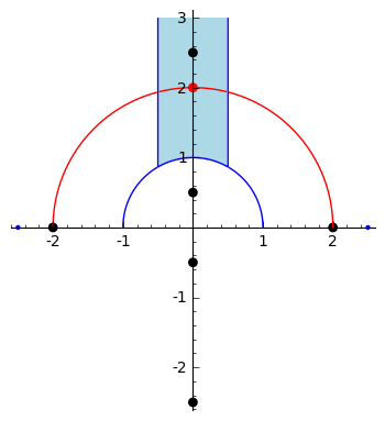
Figure 1. The image of the zero map $\zeta(f)$ is the red dot

We are denoting with black dots the roots of the form. In this case the zero map $\zeta(f)$ will be in the ”middle” of the half semicircle connecting $\pm\frac{1}{\alpha\beta}$. Since, they are symmetric with respect to the y-axis this obviously will be in the y-axis, i.e. $\zeta(f)$ is purely complex. Next, assume $\alpha$ is purely complex and $\beta$ is real. Then $\frac{1}{\alpha\beta}$ is purely complex and the proof is as above.

Now, let us assume that $\alpha$ and $\beta$ are complex roots with real and imaginary part nonzero. Then, $\beta=\bar{\alpha}$ and the set of Weierstrass points for the curve is $\{\pm\alpha,\pm\bar{\alpha},\pm\frac{1}{\alpha\bar{\alpha}}\}$. Then, the centroid of the rectangle with vertices$\{\pm\alpha,\pm\bar{\alpha}\}$ is the origin $O$. Finding the zero map $\zeta(f)$ is equivalent to finding the ”middle” of the half semicircle connecting the real roots $\pm\frac{1}{\alpha\beta}$ which will be a point in the y-axis, illustrated in Fig. (2).

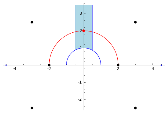
Figure 2. The image of the zero map $\zeta(f)$ is the red dot

Above we proved that $\zeta(F)$ is purely complex, i.e. $\zeta(F)=ci$ for some $c\in\mathbb{R}^{+}$. Then $f$ is reduced if and only if $c\geq 1$. Assume $f$ is not reduced. Then, there exists a binary form $g(x,z)$ such that $g(x,z)=f(-z,x)=f(z,x)$. The form $g(x,z)$ will be reduced since $\zeta(g)=-\frac{1}{\zeta(f)}=\frac{i}{c}$. Hence, either $f$ or $g$ (or possibly both, when $c=1$) will be reduced.

Lastly, if $\alpha$ and $\beta$ are both real the form $f$ is totally real. In [beshaj-thesis, Prop. 6.1 ] we proved that a superelliptic curve with such Weierstrass points is reduced in its orbit. This completes the proof. ∎

Remark 3.

After this proof was completed M. Stoll pointed out that since $\zeta(f)$ must be fixed by the extra involution $\sigma:(x,y)\to(-x,y)$. Notice that $\zeta(f)$ is uniquely determined by the coefficients $s_{1},s_{2}$. Such coefficients are fixed by the extra involution $\sigma$. Hence, $\zeta(f)$ is also fixed by such involution. Thus, $\zeta(f)$ is purely complex.

Notice that in general a binary form being reduced doesn’t necessarily mean that it has minimal height; see [reduction] for details. And an integral model of the form given as in Eq. (14) is not necessarily of minimal height among all integral models. But it is of minimal height among integral models defined by polynomials in $x^{2}$. This is proved in the following lemma.

Lemma 7.

Let $\mathcal{X}$ be a genus 2 curve with $\operatorname{Aut}({\mathfrak{p}})\simeq V_{4}$ and equation $y^{2}=f(x^{2})$, where

(16) $$f(x)=x^{6}-s_{1}x^{4}+s_{2}x^{2}-1.$$

Then, integral models of this form have minimal height among integral models defined by polynomials in $x^{2}$, even up to twist.

Proof.

Let $f(x)$ be integral given as in Eq. (16) and consider another $\mathbb{Q}$-isomorphic integral model that is a polynomial in $x^{2}$. Any such model has coefficient vector as follows

$$(\lambda^{6}\mu^{2},\lambda^{4}\mu^{2}s_{1},\lambda^{2}\mu^{2}s_{2},\mu^{2})$$

for some rational $\lambda$ and $\mu$. Now, let us proceed prime by prime. Let $v$ be the valuation of $\lambda$ and let $w$ be that of $\mu$. For the equation to have smaller height, we would need that one of the valuation jumps

$$(6v+2w,4v+2w,2v+2w,2w)$$

to be negative. But because the new model is also integral, we have $2w\geq 0$ and $6v+2w\geq 0$. However, if those two inequalities hold, then all the jumps are positive, so $4v+2w$ and $2v+2w$ as well. Therefore, our integral model of the form

(17) $$f(x)=x^{6}-s_{1}x^{4}+s_{2}x^{2}-1.$$

has minimal height among integral models defined by polynomials in $x^{2}$. ∎

Note that lots of curves with geometric automorphism group $V_{4}$ and field of moduli $\mathbb{Q}$ do not admit a model over $\mathbb{Q}$ defined by a polynomial in $x^{2}$. All of them descend, and in fact they even all descend to a hyperelliptic model instead of a cover of a conic. But they do not all admit that special form as given in Eq. (15).

The natural question is what are other additional conditions could force $f(x,z)$, where $f(x,z)$ represents the equation of a curve with extra automorphism, to be of minimal absolute height? We will elaborate more on this question in the next section.

5. Some heuristics for curves with extra involutions defined over $\mathbb{Q}$

In [alg-curves] we display a database of genus 2 curves defined over $\mathbb{Q}$. The curves in the database are ordered based on their minimal absolute height, therefore they provide a perfect case for us to check how many of our curves are in that database. In addition for each isomorphism class is given a minimal equation over the field of moduli, the automorphism group, and all the twists. All the computations involved in the database are done based on the absolute invariants $i_{1},i_{2},i_{3}$; see [alg-curves] for details. The database is explained in more details in [alg-curves].

We have added to that database even the curves discussed here defined over $\mathbb{Q}$. We have found all such curves of height $\operatorname{\mathfrak{h}}\leq 101$ defined over $\mathbb{Q}$. The number of such curves for each height $\operatorname{\mathfrak{h}}$ is displayed in the following Table 1.

In the first column is the height of the curve, the second column contains the number of tuples $(1,0,a,0,b,0,1)$ which gives a genus 2 curves (i.e. $J_{10}\neq 0$). Not all such tuples give a new moduli point. In the third column it is the number of such moduli points. The fourth and fifth column contain the number of curves with automorphism group $D_{4}$ and $D_{6}$, and the last column contains the number of all points in the moduli space of height $\leq h$.

Table 1. Number of curves with height $\operatorname{\mathfrak{h}}\leq 100$

$\operatorname{\mathfrak{h}}$	$J_{10}\neq 0$	in $\mathcal{M}_{2}$	$D_{4}$	$D_{6}$	# pts	$\operatorname{\mathfrak{h}}$	$J_{10}\neq 0$	in $\mathcal{M}_{2}$	$D_{4}$	$D_{6}$	# pts
1	8	5	1	0	5	51	10607	205	2	0	5347
2	24	9	2	0	14	52	11023	209	2	0	5556
3	47	12	1	0	26	53	11447	213	2	0	5769
4	79	17	2	0	43	54	11879	217	2	0	5986
5	119	20	1	0	63	55	12319	221	2	0	6207
6	167	25	2	0	88	56	12767	225	2	0	6432
7	223	28	1	0	116	57	13223	229	2	0	6661
8	287	33	2	0	149	58	13687	233	2	0	6894
9	359	36	1	0	185	59	14159	237	2	0	7131
10	439	41	2	0	226	60	14639	241	2	0	7372
11	527	45	2	0	271	61	15127	245	2	0	7617
12	623	49	2	0	320	62	15623	249	2	0	7866
13	727	53	2	0	373	63	16127	253	2	0	8119
14	839	57	2	0	430	64	16639	257	2	0	8376
15	959	58	1	0	488	65	17159	261	2	0	8637
16	1087	65	2	0	553	66	17687	265	2	0	8902
17	1223	68	1	0	621	67	18223	269	2	0	9171
18	1367	73	2	0	694	68	18767	273	2	0	9444
19	1519	77	2	0	771	69	19319	277	2	0	9721
20	1679	81	2	0	852	70	19879	281	2	0	10002
21	1847	85	2	0	937	71	20447	285	2	0	10287
22	2023	89	2	0	1026	72	21023	289	2	0	10576
23	2207	93	2	0	1119	73	21607	293	2	0	10869
24	2399	97	2	0	1216	74	22199	297	2	0	11166
25	2599	101	2	0	1317	75	22799	301	2	0	11467
26	2807	105	2	0	1422	76	23407	305	2	0	11772
27	3023	109	2	0	1531	77	24023	309	2	0	12081
28	3247	113	2	0	1644	78	24647	313	2	0	12394

$\operatorname{\mathfrak{h}}$	$J_{10}\neq 0$	in $\mathcal{M}_{2}$	$D_{4}$	$D_{6}$	# pts	$\operatorname{\mathfrak{h}}$	$J_{10}\neq 0$	in $\mathcal{M}_{2}$	$D_{4}$	$D_{6}$	# pts
29	3479	117	2	0	1761	79	25279	317	2	1	12711
30	3719	121	2	0	1882	80	25919	321	2	0	13032
31	3967	125	2	0	2007	81	26567	325	2	0	13357
32	4223	129	2	0	2136	82	27223	329	2	0	13686
33	4487	133	2	0	2269	83	27887	333	2	1	14019
34	4759	137	2	0	2406	84	28559	337	2	0	14356
35	5039	141	2	0	2547	85	29239	341	2	0	14697
36	5327	145	2	0	2692	86	29927	345	2	0	15042
37	5623	149	2	0	2841	87	30623	349	2	0	15391
38	5927	153	2	0	2994	88	31327	353	2	0	15744
39	6239	157	2	0	3151	89	32039	357	2	0	16101
40	6559	161	2	0	3312	90	32759	361	2	0	16462
41	6887	165	2	0	3477	91	33487	365	2	0	16827
42	7223	169	2	0	3646	92	34223	369	2	0	17196
43	7567	173	2	0	3819	93	34967	373	2	0	17569
44	7919	177	2	0	3996	94	35719	377	2	0	17946
45	8279	181	2	0	4177	95	36479	381	2	0	18327
46	8647	185	2	0	4362	96	37247	385	2	0	18712
47	9023	189	2	0	4551	97	38023	389	2	0	19101
48	9407	193	2	0	4744	98	38807	393	2	0	19494
49	9799	197	2	0	4941	99	39599	397	2	0	19891
50	10199	201	2	0	5142	100	40399	401	2	0	20292

Some interesting questions that can be addressed analyzing Table  1 are as follows. How many genus two curves with extra involutions are there with a fixed height $\operatorname{\mathfrak{h}}$? How many isomorphism classes of genus two curves with extra involutions are there for a fixed height $\operatorname{\mathfrak{h}}$? In other words, how many twists are for such curves with fixed height? We intend to further explore some of these questions in further work.

The main question that comes from the previous section was how many of these curves are of minimal absolute height. From 14523 = 20292 - 5769 binary forms of the form given in Eq. (14) we check how many of them have minimal absolute height $\leq 3$ even though $r:=\min\{|s_{1}|,|s_{2}|\}>3$. Out of 14523 forms only for 57 of them

$$r=\max\{|s_{1}|,|s_{2}|\}\neq\operatorname{\mathfrak{h}}.$$

We display all such forms in the Table  2. In the third column is the equation of the curve given the 7-tuple $(a_{0},\dots,a_{6})$ corresponding to the equation

$$y^{2}=\sum_{i=0}^{6}a_{i}x^{i}=x^{6}-s_{1}x^{4}+s_{2}x^{2}+1.$$

In the fifth column is the twist with height $\operatorname{\mathfrak{h}}\leq 4$ which is isomorphic over $\overline{\mathbb{Q}}$ with the corresponding curve in the first column. In the last column is given the automorphism group of the curve over $\overline{\mathbb{Q}}$.

Table 2. Curves which have twists with height $\leq 4$

#	$r$	$(1,0,s_{1},0,s_{2},0,1)$	$\operatorname{\mathfrak{h}}$	$(a_{0},\dots,a_{6})$	$\mbox{Aut}(\mathfrak{p})$
1	7	[1, 0, 1, 0, -7, 0, 1]	3	[1, -3, -1, -2, -1, -3, 1]	[4, 2]
2	5	[1, 0, 5, 0, 1, 0, 1]	3	[1, -1, 3, 2, 3, -1, 1]	[4, 2]
3	17	[1, 0, 15, 0, -17, 0, 1]	2	[1, -1/2, -1, -1, -1, -1/2, 1]	[4, 2]
4	29	[1, 0, -29, 0, -29, 0, 1]	3	[0, 1, 0, -3/2, 0, 1]	[8, 3]
5	9	[1, 0, 9, 0, 5, 0, 1]	2	[1, -1/2, 1, 1, 1, -1/2, 1]	[4, 2]
6	41	[1, 0, -25, 0, -41, 0, 1]	3	[1, -1/2, -3/2, 1, -3/2, -1/2, 1]	[4, 2]
7	13	[1, 0, 3, 0, -13, 0, 1]	2	[1, -2, -1, 0, -1, -2, 1]	[4, 2]
8	51	[1, 0, 51, 0, -45, 0, 1]	3	[1, 0, -1, -2/3, -1, 0, 1]	[4, 2]
9	9	[1, 0, 7, 0, -9, 0, 1]	2	[1, -1, -1, -2, -1, -1, 1]	[4, 2]
10	19	[1, 0, 19, 0, -13, 0, 1]	2	[1, 0, -1, -2, -1, 0, 1]	[4, 2]
11	61	[1, 0, 35, 0, -61, 0, 1]	3	[1, -2/3, -1, 2/3, -1, -2/3, 1]	[4, 2]
12	7	[1, 0, -7, 0, -7, 0, 1]	4	[1, 4, -3, 0, -3, -4, 1]	[8, 3]
13	61	[1, 0, 3, 0, -61, 0, 1]	3	[1, -2, -1, 3, -1, -2, 1]	[4, 2]
14	17	[1, 0, -1, 0, -17, 0, 1]	3	[1, -3, -1, 2, -1, -3, 1]	[4, 2]
15	6	[1, 0, 6, 0, 6, 0, 1]	2	[-1, 1, 1/2, 0, -1/2, -1, 1]	[8, 3]
16	13	[1, 0, -5, 0, -13, 0, 1]	3	[1, -1, -3, 2, -3, -1, 1]	[4, 2]
17	29	[1, 0, 19, 0, -29, 0, 1]	3	[1, -2/3, -1, 0, -1, -2/3, 1]	[4, 2]
18	19	[1, 0, 19, 0, 19, 0, 1]	3	[0, 1, 0, -3, 0, 1]	[8, 3]
19	5	[1, 0, -5, 0, -5, 0, 1]	1	[0, -1, 0, 0, 0, 1]	[48, 5]
20	47	[1, 0, 47, 0, 47, 0, 1]	3	[1, 0, -2/3, 0, -2/3, 0, 1]	[8, 3]
21	39	[1, 0, 39, 0, 23, 0, 1]	2	[1, -1/2, -1/2, 1, -1/2, -1/2, 1]	[4, 2]
22	5	[1, 0, 3, 0, -5, 0, 1]	2	[0, 1, -2, -2, -2, 1]	[2, 1]
23	8	[1, 0, 8, 0, 8, 0, 1]	3	[1, 1, 3/2, 0, 3/2, -1, 1]	[8, 3]
24	19	[1, 0, 19, 0, 11, 0, 1]	2	[1, -1/2, 0, 1, 0, -1/2, 1]	[4, 2]
25	21	[1, 0, -5, 0, -21, 0, 1]	4	[1, -4, -1, 4, -1, -4, 1]	[4, 2]
26	53	[1, 0, 43, 0, -53, 0, 1]	3	[1, -1/3, -1, 0, -1, -1/3, 1]	[4, 2]
27	37	[1, 0, 27, 0, -37, 0, 1]	2	[1, -1/2, -1, 0, -1, -1/2, 1]	[4, 2]
28	35	[1, 0, 35, 0, -29, 0, 1]	1	[1, 0, -1, -1, -1, 0, 1]	[4, 2]
29	93	[1, 0, 35, 0, -93, 0, 1]	3	[1, -1, -1, 3/2, -1, -1, 1]	[4, 2]
30	21	[1, 0, 11, 0, -21, 0, 1]	1	[1, -1, -1, 0, -1, -1, 1]	[4, 2]
31	55	[1, 0, 55, 0, 39, 0, 1]	3	[1, -1/3, -2/3, 2/3, -2/3, -1/3, 1]	[4, 2]
32	77	[1, 0, 51, 0, -77, 0, 1]	2	[1, -1/2, -1, 1/2, -1, -1/2, 1]	[4, 2]
33	9	[1, 0, -1, 0, -9, 0, 1]	4	[1, -4, -1, 0, -1, -4, 1]	[4, 2]
34	37	[1, 0, -37, 0, -37, 0, 1]	3	[1, 3/2, -1, 0, -1, -3/2, 1]	[8, 3]
35	11	[1, 0, 11, 0, 11, 0, 1]	3	[1, 2, 3, 0, 3, -2, 1]	[8, 3]
36	29	[1, 0, 3, 0, -29, 0, 1]	2	[1, -2, -1, 2, -1, -2, 1]	[4, 2]
37	23	[1, 0, 23, 0, 23, 0, 1]	3	[1, 0, -1/3, 0, -1/3, 0, 1]	[8, 3]
38	11	[1, 0, 5, 0, -11, 0, 1]	3	[1, -3/2, -1, -1, -1, -3/2, 1]	[4, 2]
39	11	[1, 0, 11, 0, 3, 0, 1]	2	[1, -1, 1, 2, 1, -1, 1]	[4, 2]
40	25	[1, 0, -9, 0, -25, 0, 1]	2	[1, -1, -2, 2, -2, -1, 1]	[4, 2]
41	99	[1, 0, 99, 0, -93, 0, 1]	3	[1, 0, -1, -1/3, -1, 0, 1]	[4, 2]
42	15	[1, 0, 9, 0, -15, 0, 1]	3	[1, -1, -1, -2/3, -1, -1, 1]	[4, 2]
43	23	[1, 0, 23, 0, 7, 0, 1]	2	[1, -1, 0, 2, 0, -1, 1]	[4, 2]
44	45	[1, 0, 19, 0, -45, 0, 1]	1	[1, -1, -1, 1, -1, -1, 1]	[4, 2]
45	31	[1, 0, 31, 0, 31, 0, 1]	2	[1, 0, -1/2, 0, -1/2, 0, 1]	[8, 3]
46	9	[1, 0, 9, 0, 9, 0, 1]	3	[-1, -3, -3, -2, 3, -3, 1]	[8, 3]
47	25	[1, 0, 7, 0, -25, 0, 1]	3	[1, -3/2, -1, 1, -1, -3/2, 1]	[4, 2]
48	83	[1, 0, 83, 0, -45, 0, 1]	3	[1, -1/2, -1, 3/2, -1, -1/2, 1]	[4, 2]
49	13	[1, 0, 13, 0, 9, 0, 1]	3	[1, -1/3, 1/3, 2/3, 1/3, -1/3, 1]	[4, 2]

50	25	[1, 0, 23, 0, -25, 0, 1]	3	[1, -1/3, -1, -2/3, -1, -1/3, 1]	[4, 2]
51	33	[1, 0, 15, 0, -33, 0, 1]	3	[1, -1, -1, 2/3, -1, -1, 1]	[4, 2]
52	27	[1, 0, 27, 0, 19, 0, 1]	3	[1, -1/3, -1/3, 2/3, -1/3, -1/3, 1]	[4, 2]
53	51	[1, 0, 51, 0, -13, 0, 1]	3	[1, -1, -1, 3, -1, -1, 1]	[4, 2]
54	13	[1, 0, -13, 0, -13, 0, 1]	1	[0, 1, 0, -1, 0, 1]	[8, 3]
55	27	[1, 0, 27, 0, 27, 0, 1]	3	[1, 3, 3, 0, 3, -3, 1]	[8, 3]
56	67	[1, 0, 67, 0, -61, 0, 1]	2	[1, 0, -1, -1/2, -1, 0, 1]	[4, 2]
57	33	[1, 0, -33, 0, -33, 0, 1]	3	[1, 0, -3/2, 0, -3/2, 0, 1]	[8, 3]

There are a few questions which arise from Table 2. First, can the curves of column five be obtained from reducing curves of column three? Secondly, are they in the same $\Gamma$-orbit as the curves from column 2?

In response to this question, we found that twenty of the curves displayed in Table 2 can be reduced further using the reduction algorithm. They are displayed in Table 3. In the second column is displayed the curve from Table 2, in the third column the curve obtained by the reduction algorithm and the last column the automorphism group of the curve. Some of the reduced curves are isomorphic to the original curves over $\mathbb{Q}$.

Table 3. Curves which have twists with height $\leq 4$ and reduced curves.

case #	$(s_{1},s_{2})$-curve	reduced curve	Group
57	(1, 0, -33, 0, -33, 0, 1)	( -2, 0, 3, 0, 3, 0, -2)	[8, 3]
50	( 1 , 0, 23, 0, -25, 0, 1 )	( 0 , 3, 1, -6, 1, 3, 0)	[4, 2]
21	( 1 , 0, 39, 0, 23, 0, 1 )	( 2, 1, -1, -2, -1, 1, 2 )	[4, 2]
16	( 1 , 0, -5, 0, -13, 0, 1 )	( -1, -1, 3, 2, 3, -1, -1 )	[4, 2]
20	( 1 , 0, 47, 0, 47, 0, 1 )	( 3, 0, -2, 0, -2, 0, 3 )	[8, 3]
39	( 1 , 0, 11, 0, 3, 0, 1 )	( 1 , -1, 1, 2, 1, -1, 1 )	[4, 2]
3	( 1 , 0, 15, 0, -17, 0, 1 )	( 0, 2, 1, -4, 1, 2, 0 )	[4, 2]
47	( 1 , 0, 7, 0, -25, 0, 1 )	( 1, -4, 3, 8, 3, -4, -1 )	[4, 2]
40	( 1 , 0, -9, 0, -25, 0, 1 )	( -1, -1, 2, 2, 2, -1, -1 )	[4, 2]
24	( 1 , 0, 19, 0, 11, 0, 1 )	( 2, 1, 0, -2, 0, 1, 2 )	[4, 2]
9	( 1 , 0, 7, 0, -9, 0, 1 )	( 0, -1, 1, 2, 1, -1, 0 )	[4, 2]
37	( 1 , 0, 23, 0, 23, 0, 1 )	( 3, 0, -1, 0, -1, 0, 3 )	[8, 3]
43	( 1 , 0, 23, 0, 7, 0, 1 )	( 1 , -1, 0, 2, 0, -1, 1 )	[4, 2]
31	( 1 , 0, 55, 0, 39, 0, 1 )	( 3, 1, -2, -2, -2, 1, 3 )	[4, 2]
6	( 1 , 0, -25, 0, -41, 0, 1 )	( -2, 1, 3, -2, 3, 1, -2 )	[4, 2]
45	( 1 , 0, 31, 0, 31, 0, 1 )	(2, 0, -1, 0, -1, 0, 2 )	[8, 3]
52	( 1 , 0, 27, 0, 19, 0, 1 )	( 3, 1, -1, -2, -2, 1, 3 )	[4, 2]
14	( 1 , 0, -1, 0, -17, 0, 1 )	( -1, 2, 3, -4, 3, 2, -1 )	[4, 2]
51	( 1 , 0, 15, 0, -33, 0, 1 )	(-1, -6, 3, 12, 3, -6, 1 )	[4, 2]

It is worth noting that in each case the reduction algorithm does find a curve with minimal absolute height. It is also interesting to see that all 57 curves from Table 2 have one thing in common, their discriminant can be further reduced as explained in Section (3.4).

We believe that a generalization of Thm. 3 to higher degree binary forms $f(x^{2},y^{2})$ and in more general for forms $f(x^{n},y^{n})$ is possible. Hopefully, this will be the focus of investigation of another paper.

Acknowledgments: I would like to thank M. Stoll, T. Shaska, and J. Sijsling for valuable comments and help. Furthermore, I would like to thank the anonymous referees for all the comments they provided during the review.