In-Medium Similarity Renormalization Group Approach to the Nuclear Many-Body Problem

Abstract

We present a pedagogical discussion of Similarity Renormalization Group (SRG) methods, in particular the In-Medium SRG (IMSRG) approach for solving the nuclear many-body problem. These methods use continuous unitary transformations to evolve the nuclear Hamiltonian to a desired shape. The IMSRG, in particular, is used to decouple the ground state from all excitations and solve the many-body Schrödinger equation. We discuss the IMSRG formalism as well as its numerical implementation, and use the method to study the pairing model and infinite neutron matter. We compare our results with those of Coupled cluster theory (Chapter 8), Configuration-Interaction Monte Carlo (Chapter 9), and the Self-Consistent Green’s Function approach discussed in Chapter 11. The chapter concludes with an expanded overview of current research directions, and a look ahead at upcoming developments.

9.1 Introduction

Effective Field Theory (EFT) and Renormalization Group (RG) methods have become important tools of modern (nuclear) many-body theory — one need only look at the table of contents of this book to see the veracity of this claim.

Effective Field Theories allow us to systematically take into account the separation of scales when we construct theories to describe natural phenomena. One of the earliest examples that every physics student encounters is the effective force law of gravity near the surface of the Earth: For a mass $m$ at a height $h$ above ground, Newton’s force law becomes

$$F(R+h)=G\frac{mM}{(R+h)^{2}}=m\frac{GM}{R^{2}}\frac{1}{1+\left(\frac{h}{R}\right)^{2}}=m\underbrace{\frac{GM}{R^{2}}}_{\equiv g}+\mathscr{O}\left(\frac{h^{2}}{R^{2}}\right)\,,$$ (9.1)

where $M$ and $R$ are the mass and radius of the Earth, respectively. Additional examples are the multipole expansion of electric fields Jackson:1999yg , which shows that only the moments of an electric charge distribution with characteristic length scale $R$ are resolved by probes with long wave lengths $\lambda\gg R$, or Fermi’s theory of beta decay Fermi:1934eu , which can nowadays be derived from the Standard Model by expanding the propagator of the $W^{\pm}$ bosons that mediate weak processes for small momenta $q\ll M_{W}=80\,\,\text{GeV}$ (in units where $\hbar=c=1$).

The strong-interaction sector of the Standard Model is provided by Quantum Chromodynamics (QCD), but the description of nuclear observables on the level of quarks and gluons is not feasible, except in the lightest few-nucleon systems (see, e.g., Detmold:2015xw and the chapters on Lattice QCD in this book). The main issue is that QCD is an asymptotically free theory Gross:1973pd ; Politzer:1973lq , i.e., it is weak and amenable to perturbative methods from Quantum Field Theory at large momentum transfer, but highly non-perturbative in the low-momentum regime which is relevant for nuclear structure physics. A consequence of the latter property is that quarks are confined in baryons and mesons at low momentum or energy scales, which makes those confined particles suitable degrees of freedom for an EFT approach. Chiral EFT, in particular, is constructed in terms of nucleon and pion fields, with some attention now also being given to the lowest excitation mode of the nucleon, namely the $\Delta$ resonance. It provides provides a constructive framework and organizational hierarchy for $NN$, $3N$, and higher many-nucleon forces, as well as consistent electroweak operators (see, e.g., Epelbaum:2009ve ; Machleidt:2011bh ; Epelbaum:2015gf ; Entem:2015qf ; Gezerlis:2014zr ; Lynn:2016ec ; Pastore:2009zr ; Pastore:2011dq ; Piarulli:2013vn ; Kolling:2009yq ; Kolling:2011bh ). Since Chiral EFT is a low-momentum expansion, high-momentum (short-range) physics is not explicitly resolved by the theory, but parametrized by the so-called low-energy constants (LECs). In principle, the LECs can be determined by matching calculations of the same observables in chiral EFT and (Lattice) QCD in the overlap region of the two theories. Since such a calculation is currently not feasible, they are fit to experimental data for low-energy QCD observables, typically in the $\pi{}N$, $NN$, and $3N$ sectors Epelbaum:2009ve ; Machleidt:2011bh ; Ekstrom:2015fk ; Shirokov:2016wo .

RG methods are natural companions for EFTs, because smoothly connect theories with different resolution scales and degrees of freedom Lepage:1989hf ; Lepage:1997py . Since they were introduced in low-energy nuclear physics around the start of the millennium Bogner:2003os ; Bogner:2007od ; Bogner:2010pq ; Furnstahl:2013zt , they have provided a systematic framework for formalizing many ideas on the renormalization of nuclear interactions and many-body effects that had been discussed in the nuclear structure community since the 1950s. For instance, soft and hard-core $NN$ interactions can reproduce scattering data equally well, but have significantly different saturation properties, which caused the community to all but abandon the former in the 1970s (see, e.g., Bethe:1971qf ). What was missing at that time was the recognition of the intricate link between the off-shell $NN$ interaction and $3N$ forces that was formally demonstrated for the first time by Polyzou and Glöckle in 1990 Polyzou:1990fk . From the modern RG perspective, soft- and hard-core interactions emerge as representations of low-energy QCD at different resolution scales, and the dialing of the resolution scale necessarily leads to induced $3N$ forces, in such a way that observables (including saturation properties) remain invariant under the RG flow (see Sec. 9.2.4 and Bogner:2010pq ; Furnstahl:2013zt ). In conjunction, chiral EFT and nuclear RG applications demonstrate that one cannot treat the $NN,3N,\ldots$ sectors in isolation from each other.

Brueckner introduced the idea of renormalizing the $NN$ interaction in the nuclear medium by summing correlations due to the scattering of nucleon pairs to high-energy states into the so-called $G$-matrix, which became the basis of an attempted perturbation expansion of nuclear observables Brueckner:1954qf ; Brueckner:1955rw ; Bethe:1957qv ; Goldstone:1957zz ; Day:1967zl ; Brandow:1967tg . Eventually, the nuclear structure community uncovered severe issues with this approach, like a lack of order-by-order convergence Barrett:1970jl ; Kirson:1971la ; Barrett:1972bs ; Kirson:1974oq ; Goode:1974pi , and a strong model space dependence in summations over virtual excitations Vary:1973dn . One of the present authors led a study that revisited this issue, and demonstrated that the $G$ matrix retains significant coupling between low- and high-momentum nodes of the underlying interaction Bogner:2010pq , so the convergence issues are not surprising from a modern perspective. In the Similarity Renormalization Group Glazek:1993il ; Wegner:1994dk and other modern RG approaches, low- and high-momentum physics are decoupled properly, which results in low-momentum interactions that can be treated successfully in finite-order many-body perturbation theory (MBPT) Bogner:2006qf ; Bogner:2010pq ; Roth:2010ys ; Tichai:2016vl . These interactions are not just suited as input for MBPT, but for all methods that work with momentum- or energy-truncated configuration spaces. The decoupling of low- and high-momentum modes greatly improves the convergence behavior of such methods, which can then be applied to heavier and heavier nuclei Barrett:2013oq ; Jurgenson:2013fk ; Hergert:2013ij ; Roth:2014fk ; Binder:2014fk ; Hagen:2014ve ; Hagen:2016rb .

The idea of decoupling energy scales can also be used to directly tackle the nuclear many-body problem. We implement it in the so-called In-Medium SRG Tsukiyama:2011uq ; Hergert:2013mi ; Hergert:2016jk , which is discussed at length in this chapter. In a nutshell, we will use SRG-like flow equations to decouple physics at different excitation energy scales of the nucleus, and render the Hamiltonian matrix in configuration space block or band diagonal in the process. We will see that this can be achieved while working on the operator level, freeing us from the need to construct the Hamiltonian matrix in a factorially growing basis of configurations. We will show that the IMSRG evolution can also be viewed as a re-organization of the many-body perturbation series, in which correlations that are described explicitly by the configuration space are absorbed into an RG-improved Hamiltonian. With an appropriately chosen decoupling strategy, it is even possible to extract specific eigenvalues and eigenstates of the Hamiltonian, which is why the IMSRG qualifies as an ab initio (first principles) method for solving quantum many-body problems.

The idea of using flow equations to solve quantum many-body problems dates back (at least) to Wegner’s initial work on the SRG Wegner:1994dk (also see Kehrein:2006kx and references therein). In the solid-state physics literature, the approach is also known as continuous unitary transformation theory Heidbrink:2002kx ; Drescher:2011kx ; Krull:2012bs ; Fauseweh:2013zv ; Krones:2015ft . When we discuss our decoupling strategies for the nuclear many-body problem, it will become evident that the IMSRG is related to Coupled Cluster theory (CC), see also chapter 8, and a variety of other many-body methods that are used heavily in quantum chemistry (see, e.g., Shavitt:2009 ; Hagen:2014ve ; White:2002fk ; Yanai:2007kx ; Nakatsuji:1976yq ; Mukherjee:2001uq ; Mazziotti:2006fk ; Evangelista:2014rq ). What sets the IMSRG apart from these methods is that the Hamiltonian instead of the wave function is at the center of attention, in the spirit of RG methodology. This seems to be a trivial distinction, but there are practical advantages of this viewpoint, like the ability to simultaneously decouple ground and a number of excited states from the rest of the spectrum (see Secs. 9.3.3 and 9.4.3).

Organization of this Chapter

We conclude our introduction by looking ahead at the remainder of this chapter. In Sec. 9.2, we will introduce the basic concepts of the SRG, and apply it to a pedagogical toy model (Sec. 9.2.2), the pairing Hamiltonian that is also discussed in Chapters 8, 9, and 11 (Sec. 9.2.3), and last but not least, we will discuss the SRG evolution of modern nuclear interactions (Sec. 9.2.4).

The issue of SRG-induced operators (Sec. 9.2.4) will serve as our launching point for the discussion of the IMSRG in Sec. 9.3. First, we will introduce normal-ordering techniques as a means to control the size of induced interaction terms (Sec. 9.3.1). This is followed by the derivation of the IMSRG flow equations, determination of decoupling conditions, and the construction of generators in Secs. 9.3.2–9.3.4. We discuss the essential steps of an IMSRG implementation through the example of a symmetry-unconstrained Python code (Sec. 9.3.5), and use this code to revisit the pairing Hamiltonian in Sec. 9.3.6. In Sec. 9.3.7, we compute the neutron matter equation-of-state in the IMSRG(2) truncation scheme, and compare our result to that of corresponding Coupled Cluster, Quantum Monte Carlo, and Self-Consistent Green’s Function results with the same interaction.

Section 9.4 introduces the three major directions of current research: First, we present the Magnus formulation of the IMSRG (Sec. 9.4.1), which is the key to the efficient computation of observables and the construction of approximate version of the IMSRG(3). Second, we give an overview of the multireference IMSRG (MR-IMSRG), which generalizes our framework to arbitrary reference states, and gives us new freedom to manipulate the correlation content of our many-body calculations 9.4.2. Third, we will discuss applications of IMSRG-evolved, RG-improved Hamiltonians as input to many-body calculations, in particular for the nuclear (interacting) Shell model and Equation-of-Motion (EOM) methods (Sec. 9.4.3). An outlook on how these three research thrusts interweave concludes the section (Sec. 9.4.4).

In Sec. 9.5, we make some final remarks and close the main body of the chapter in Sec. 9.5. Section 9.6 contains exercises that further flesh out subjects discussed in the preceding sections, as well as outlines for computational projects. Formulas for products and commutators of normal-ordered operators are collected in an Appendix.

9.2 The Similarity Renormalization Group

9.2.1 Concept

The basic idea of the Similarity Renormalization Group (SRG) method is quite general: We want to “simplify” our system’s Hamiltonian $\hat{H}(s)$ by means of a continuous unitary transformation that is parametrized by a one-dimensional parameter $s$,

$$\hat{H}(s)=\hat{U}(s)\hat{H}(0)\hat{U}^{\dagger}(s)\,.$$ (9.2)

By convention, $\hat{H}(s=0)$ is the starting Hamiltonian. To specify what we mean by simplifying $\hat{H}$, it is useful to briefly think of it as a matrix rather than an operator. As in any quantum-mechanical problem, we are primarily interested in finding the eigenstates of $\hat{H}$ by diagonalizing its matrix representation. This task is made easier if we can construct a unitary transformation that renders the Hamiltonian more and more diagonal as $s$ increases. Mathematically, we want to split the Hamiltonian into suitably defined diagonal and off-diagonal parts,

$$\hat{H}(s)=\hat{H}_{d}(s)+\hat{H}_{od}(s)\,,$$ (9.3)

and find $\hat{U}(s)$ so that

$$\hat{H}(s)\underset{s\to\infty}{\longrightarrow}\hat{H}_{d}(s)\,,\quad\hat{H}_{od}(s)\underset{s\to\infty}{\longrightarrow}0\,.$$ (9.4)

To implement the continuous unitary transformation, we take the derivative of Eq. (9.2) with respect to $s$ to obtain

$$\frac{d{\hat{H}(s)}}{d{s}}=\frac{d{\hat{U}(s)}}{d{s}}\hat{H}(0)\hat{U}^{\dagger}(s)+\hat{U}(s)\hat{H}(0)\frac{d{\hat{U}^{\dagger}(s)}}{d{s}}=\frac{d{\hat{U}(s)}}{d{s}}\hat{U}^{\dagger}(s)\hat{H}(s)+\hat{H}(s)\hat{U}(s)\frac{d{\hat{U}^{\dagger}(s)}}{d{s}}\,.$$ (9.5)

Since $\hat{U}(s)$ is unitary, we also have

$$\frac{d{}}{d{s}}\left(\hat{U}(s)\hat{U}^{\dagger}(s)\right)=\frac{d{}}{d{s}}\left(\hat{I}\right)=0\quad\Longrightarrow\quad\frac{d{\hat{U}(s)}}{d{s}}\hat{U}^{\dagger}(s)=-\hat{U}(s)\frac{d{\hat{U}^{\dagger}(s)}}{d{s}}\,.$$ (9.6)

Defining the anti-Hermitian operator

$$\hat{\eta}(s)\equiv\frac{d{\hat{U}(s)}}{d{s}}\hat{U}^{\dagger}(s)=-\hat{\eta}^{\dagger}(s)\,,$$ (9.7)

we can write the differential equation for the $s$-dependent Hamiltonian as

$$\frac{d{}}{d{s}}\hat{H}(s)=[{\hat{\eta}(s)},{\hat{H}(s)}]\,.$$ (9.8)

This is the SRG flow equation for the Hamiltonian, which describes the evolution of $\hat{H}(s)$ under the action of a dynamical generator $\hat{\eta}(s)$. Since we are considering a unitary transformation, the spectrum of the Hamiltonian is preserved. Thus, the SRG is related to so-called isospectral flows, a class of transformations that has been studied extensively in the mathematics literature (see for example Refs. Brockett:1991kx ; Chu:1994vn ; Chu:1995ys ; Bach:2010zr ; Boutin:2016ef ).

The flow equation (9.8) is the most practical way of implementing an SRG evolution: We can obtain $\hat{H}(s)$ by integrating Eq. (9.8) numerically, without explicitly constructing the unitary transformation itself. Formally, we can also obtain $\hat{U}(s)$ by rearranging Eq. (9.7) into

$$\frac{d{}}{d{s}}\hat{U}(s)=\hat{\eta}(s)\hat{U}(s)\,.$$ (9.9)

The solution to this differential equation is given by the $S$-ordered exponential

$$U(s) =\mathscr{S}\exp\int^{s}_{0}ds^{\prime}\,\eta(s^{\prime})\,,$$ (9.10)

because the generator changes dynamically during the flow. This expression is defined equivalently either as a product of infinitesimal unitary transformations,

$$U(s) =\lim_{N\to\infty}\prod^{N}_{i=0}e^{\eta(s_{i})\delta s_{i}}\,,\quad s_{i+1}=s_{i}+\delta s_{i}\,,\quad\sum_{i}\delta s_{i}=s\,,$$ (9.11)

or through a series expansion:

$$U(s) =\sum_{n}\frac{1}{n!}\int^{s}_{0}ds_{1}\int^{s}_{0}ds_{2}\ldots\int^{s}_{0}ds_{n}\mathscr{S}\{\eta(s_{1})\ldots\eta(s_{n})\}\,.$$ (9.12)

Here, the $S$-ordering operator $\mathscr{S}$ ensures that the flow parameters appearing in the integrands are always in descending order, $s_{1}>s_{2}>\ldots$. Note that neither Eq. (9.11) nor Eq. (9.12) can be written as a single proper exponential, so we do not obtain a simple Baker-Campbell-Hausdorff expansion of the transformed Hamiltonian. Instead, we would have to use these complicated expressions to construct $\hat{H}(s)=\hat{U}(s)\hat{H}(0)\hat{U}^{\dagger}(s)$, and to make matters even worse, Eqs. (9.11) and (9.12) depend on the generator at all intermediate points of the flow trajectory. The associated storage needs would make numerical applications impractical or entirely unfeasible.

Let us focus on the flow equation (9.8), then, and specify a generator that will transform the Hamiltonian to the desired structure (Eq. (9.4)). Inspired by the work of Brockett Brockett:1991kx on the so-called double-bracket flow, Wegner Wegner:1994dk proposed the generator

$$\hat{\eta}(s)\equiv[{H_{d}(s)},{H_{od}(s)}]\,.$$ (9.13)

A fixed point of the SRG flow is reached when $\hat{\eta}(s)$ vanishes. At finite $s$, this can occur if $\hat{H}_{d}(s)$ and $\hat{H}_{od}(s)$ happen to commute, e.g., due to a degeneracy in the spectrum of $\hat{H}(s)$. A second fixed point at $s\to\infty$ exists if $\hat{H}_{od}(s)$ vanishes as required.

Going back over the discussion, you may notice that we never specified in detail how we split the Hamiltonian into diagonal and off-diagonal parts. By “diagonal” we really mean the desired structure of the Hamiltonian, and “off-diagonal” labels the contributions we have to suppress in the limit $s\to\infty$ to obtain that structure. The basic concepts described here are completely general, and we will discuss two examples in which we apply them to the diagonalization of matrices in the following. The renormalization of Hamiltonians (or other operators) is a more specific application of continuous unitary transformations. We make contact with renormalization ideas by imposing a block or band-diagonal structure on the representation of operators in bases that are organized by momentum or energy. This implies a decoupling of low and high momenta or energies in the renormalization group sense. We will conclude this section with a brief discussion of how this SRG decoupling of scales is used to render nuclear Hamiltonians more suitable for ab initio many-body calculations Bogner:2007od ; Bogner:2010pq ; Morris:2015ve ; Hergert:2016jk ; Hergert:2017kx .

9.2.2 A Two-Dimensional Toy Problem

In order to get a better understanding of the SRG method, we first consider a simple $2\times 2$ matrix problem that can be solved analytically, and compare the flow generated by Eq. (9.8) with standard diagonalization algorithms like Jacobi’s rotation method (see, e.g., Ref. Golub:2013le ).

Let us consider a symmetric matrix $H$,

$$H\equiv\begin{pmatrix}H_{11}&H_{12}\\ H_{12}&H_{22}\end{pmatrix}.$$ (9.14)

and an orthogonal (i.e., unitary and real) matrix $U$,

$$U=\begin{pmatrix}\cos\gamma&\sin\gamma\\ -\sin\gamma&\cos\gamma\end{pmatrix},$$ (9.15)

that parameterizes a rotation of the basis in which $H$ and $U$ are represented. We want to find an angle $\gamma$ so that $H^{\prime}=UHU^{T}$ is diagonal, and to achieve this, we need to solve

$$(H_{22}-H_{11})\cos\gamma\,\sin\gamma+H_{12}(\cos^{2}\gamma-\sin^{2}\gamma)=0\,.$$ (9.16)

Using the addition theorems $\cos^{2}\gamma-\sin^{2}\gamma=\cos(2\gamma)$ and $\cos\gamma\,\sin\gamma=\sin(2\gamma)/2$, we can rewrite this equation as

$$\tan(2\gamma)=\frac{2H_{12}}{H_{11}-H_{22}}$$ (9.17)

and obtain

$$\gamma=\frac{1}{2}\tan^{-1}\left(\frac{2H_{12}}{H_{11}-H_{22}}\right)+\frac{k\pi}{2},\quad k\in\mathbb{Z},$$ (9.18)

where $k\pi/2$ is added due to the periodicity of the $\tan$ function. Note that $k=0$ gives a diagonal matrix of the form

$$H^{\prime}_{k=0}=\begin{pmatrix}E_{1}&0\\ 0&E_{2}\end{pmatrix},$$ (9.19)

while $k=1$ interchanges the diagonal elements:

$$H^{\prime}_{k=1}=\begin{pmatrix}E_{2}&0\\ 0&E_{1}\end{pmatrix}.$$ (9.20)

Let us now solve the same problem with an SRG flow. We parameterize the Hamiltonian as

$$H(s)=H_{d}(s)+H_{od}(s)\equiv\begin{pmatrix}E_{1}(s)&0\\ 0&E_{2}(s)\end{pmatrix}+\begin{pmatrix}0&V(s)\\ V(s)&0\end{pmatrix}\,,$$ (9.21)

working in the eigenbasis of $H_{d}(s)$. We can express $H(s)$ in terms of the $2\times 2$ identity matrix and the Pauli matrices:

$$H(s)=E_{+}(s)\hat{I}+E_{-}(s)\sigma_{3}+V(s)\sigma_{1}\,,$$ (9.22)

where we have introduced

$$E_{\pm}(s)\equiv\frac{1}{2}\left(E_{1}(s)\pm E_{2}(s)\right)\,.$$ (9.23)

The Wegner generator can be determined readily using the algebra of the Pauli matrices, $[{\sigma_{j}},{\sigma_{k}}]=2i\varepsilon_{jkl}\sigma_{l}$:

$$\eta(s)=[{H_{d}(s)},{H_{od}(s)}]=2iE_{-}(s)V(s)\sigma_{2}\,.$$ (9.24)

By evaluating both $\dot{H}(s)$ as well as $[{\hat{\eta}(s)},{\hat{H}(s)}]$ and comparing the coefficients of the $2\times 2$ matrices, we obtain the following system of flow equations:

$$\dot{E}_{+} =0$$ (9.25)

$$\dot{E}_{-} =4V^{2}E_{-}$$ (9.26)

$$\dot{V} =-4E_{-}^{2}V\,,$$ (9.27)

where we have suppressed the flow parameter dependence for brevity. The first flow equation reflects the conservation of the Hamiltonian’s trace under unitary transformations,

$$\mathrm{tr}\,(E_{1}(s)+E_{2}(s))=\mathrm{tr}\,(E_{1}(0)+E_{2}(0))=\text{const.}$$ (9.28)

The third flow equation can be rearranged into

$$\frac{1}{V}dV=-4E_{-}^{2}ds$$ (9.29)

and integrated, which yields

$$V(s)=V(0)\exp\left(-4\int_{0}^{s}ds^{\prime}\,E^{2}_{-}(s^{\prime})\right)\,.$$ (9.30)

Since $E_{-}(s)$ is real, the integral is positive for all values of $s$, and this means that the off-diagonal matrix element will be suppressed exponentially as we evolve $s\to\infty$ (barring singular behavior in $E_{\pm}(s)$).

To proceed, we introduce new variables $\Omega$ and $\theta$:

$$\Omega\equiv\sqrt{E_{-}^{2}+V^{2}}\,,\quad\tan\frac{\theta}{2}\equiv\frac{V}{E_{-}}\,.$$ (9.31)

Using Eqs. (9.26) and (9.27), we can show that $\Omega$ is a flow invariant:

$$\dot{\Omega}=\frac{1}{2\Omega}(2E_{-}\dot{E}_{-}+2V\dot{V})=0\,.$$ (9.32)

Rewriting $E_{-}(s)$ and $V(s)$ in terms of $\Omega$ and $\theta(s)$, we then have

$$E_{-}(s)=\Omega\cos\frac{\theta(s)}{2}\,,\quad V(s)=\Omega\sin\frac{\theta(s)}{2}\,.$$ (9.33)

Using these expressions, we find that Eqs. (9.26) and (9.27) reduce to a single differential equation for $\theta(s)$:

$$\dot{\theta}=-8\Omega^{2}\sin\frac{\theta(s)}{2}\cos\frac{\theta(s)}{2}=-4\Omega^{2}\sin\theta\,.$$ (9.34)

Bringing $\sin\theta$ to the left-hand side and using

$$\frac{d{}}{d{x}}\ln\tan\frac{x}{2}=\frac{1}{\sin x}\,,$$ (9.35)

we can integrate the ordinary differential equation (ODE) and obtain

$$\tan\frac{\theta(s)}{2}=\tan\frac{\theta(0)}{2}e^{-4\Omega^{2}s}\,.$$ (9.36)

At $s=0$ we have

$$\theta(0)=2\tan^{-1}\frac{V(0)}{E_{-}(0)}+2k\pi=2\tan^{-1}\frac{2V(0)}{E_{1}(0)-E_{2}(0)}+2k\pi\,,\quad k\in\mathbb{Z}\,,$$ (9.37)

which is just four times the angle of the Jacobi rotation that diagonalizes our initial matrix, Eq. (9.18). Likewise $\theta(s)$ is (up to the prefactor) the angle of the Jacobi rotation that will diagonalize the evolved $H(s)$ for $s>0$. In the limit $s\to\infty$, $\theta(s)\to 0$ because the SRG flow has driven the off-diagonal matrix element to zero and the Hamiltonian is already diagonal.

When we introduced the parameterization (9.33), we chose $\Omega$ to be positive, which means that $\theta(s)$ must encode all information on the signs of $E_{-}(s)$ and $V(s)$. In Fig. 9.1, we show these quantities as a function of $\theta(s)$ over the interval $[0,4\pi]$. We see that the four possible sign combinations correspond to distinct regions in the interval. We can map any set of initial values — or any point of the flow, really — to a distinct value $\theta(s)$ in this figure, even in limiting cases: For instance, if the diagonal matrix elements are degenerate, $E_{1}=E_{2}$, we have $E_{-}=0$, the angle $\theta$ will approach $\pm\pi$ and $V(s)/\Omega\to\pm 1$. From this point the SRG flow will drive $E_{-}(s)$ and $V(s)$ to the nearest fixed point at a multiple of $2\pi$ according to the trajectory for $\theta(s),$Eq. (9.36). The fixed points and flow directions are indicated in the figure.

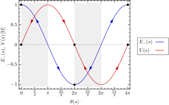
Figure 9.1: $E_{-}(s)$ and $V(s)$ as a function of the flowing angle $\theta(s)$, in units of the flow invariant $\Omega$. Black dots and arrows the fixed points at $s\to\infty$ and the directions of the SRG flow, respectively, in the domains corresponding to specific sign combinations for $E_{-}(s)$ and $V(s)$ (see text).

9.2.3 The Pairing Model

Preliminaries

state	$p$	$2s_{z}$	$\varepsilon$
$0$	$1$	$1$	$0$
$1$	$1$	$-1$	$0$
$2$	$2$	$1$	$\delta$
$3$	$2$	$-1$	$\delta$
$4$	$3$	$1$	$2\delta$
$5$	$3$	$-1$	$2\delta$
$6$	$4$	$1$	$3\delta$
$7$	$4$	$-1$	$3\delta$

Table 9.1: Single-particle states and their quantum numbers and their energies from Eq. (9.38). The degeneracy for every quantum number $p$ is equal to 2 due to the two possible spin values.

As our second example for diagonalizing matrices by means of SRG flows, we will consider the pairing model that was discussed in the context of Hartree-Fock and beyond-HF methods in chapter 8. In second quantization, the pairing Hamiltonian is given by

$$\hat{H}=\delta\sum_{p\sigma}(p-1)a^{\dagger}_{p\sigma}a_{p\sigma}-\frac{1}{2}g\sum_{pq}a^{\dagger}_{p+}a^{\dagger}_{p-}a_{q-}a_{q+}\,,$$ (9.38)

where $\delta$ controls the spacing of single-particle levels that are indexed by a principal quantum number $p=0,\ldots,3$ and their spin projection $\sigma$ (see Tab. 9.1), and $g$ the strength of the pairing interaction.

We will consider the case of four particles in eight single-particle states. Following the Full Configuration Interaction (FCI) approach discussed in Chap. 8, we can construct a many-body basis of Slater determinants by placing our particles into the available single-particle basis states. Since each single-particle state can only be occupied by one particle, there are

$$\begin{pmatrix}8\\ 4\end{pmatrix}=70$$ (9.39)

unique configurations. The specific form of the pairing interaction implies that the total spin projection $S_{z}=\sum_{n=1}^{4}s_{z}^{(n)}$ is conserved, and the Hamiltonian will have a block diagonal structure. The possible values for $S_{z}$ are $-2,-1,0,1,2$, depending on the number of particles in states with spin up ($N_{+}$) or spin down ($N_{-}$). The dimension can be calculated via

$$d_{S_{z}}=\begin{pmatrix}4\\ N_{+}\end{pmatrix}\times\begin{pmatrix}4\\ N_{-}\end{pmatrix}\,,$$ (9.40)

which yields

$$d_{\pm 2}=1\,,\quad d_{\pm 1}=16\,,\quad d_{0}=36\,.$$ (9.41)

Since the pairing interaction only couples pairs of single-particle states with the same principal quantum number but opposite spin projection, it does not break pairs of particles that occupy such states — in other words, the number of particle pairs is another conserved quantity, which allows us to decompose the $S_{z}$ blocks into even smaller sub blocks. As in chapter 8, we consider the $S_{z}=0$ sub block with two particle pairs. In this block, the Hamiltonian is represented by the six-dimensional matrix (suppressing block indices)

$$H=\begin{pmatrix}2\delta-g&-g/2&-g/2&-g/2&-g/2&0\\ -g/2&4\delta-g&-g/2&-g/2&-0&-g/2\\ -g/2&-g/2&6\delta-g&0&-g/2&-g/2\\ -g/2&-g/2&0&6\delta-g&-g/2&-g/2\\ -g/2&0&-g/2&-g/2&8\delta-g&-g/2\\ 0&-g/2&-g/2&-g/2&-g/2&10\delta-g\end{pmatrix}\,.$$ (9.42)

SRG Flow for the Pairing Hamiltonian

As in earlier sections, we split the Hamiltonian matrix (9.42) into diagonal and off-diagonal parts:

$$H_{d}(s)=\mathrm{diag}(E_{0}(s)\,,\ldots,E_{5}(s))\,,\quad H_{od}(s)=H(s)-H_{d}(s)\,,$$ (9.43)

with initial values defined by Eq. (9.42). Since $H_{d}(s)$ is diagonal throughout the flow per construction, the Slater determinants that span our specific subspace are the eigenstates of this matrix. In our basis representation, Eq. (9.8) can be written as

$$\frac{d{}}{d{s}}\langle{i}|\,{\hat{H}}\,|{j}\rangle =\sum_{k}\left(\langle{i}|\,{\hat{\eta}}\,|{k}\rangle\langle{k}|\,{\hat{H}}\,|{j}\rangle-\langle{i}|\,{\hat{H}}\,|{k}\rangle\langle{k}|\,{\hat{\eta}}\,|{j}\rangle\right)$$

$$=-\left(E_{i}-E_{j}\right)\langle{i}|\,{\hat{\eta}}\,|{j}\rangle+\sum_{k}\left(\langle{i}|\,{\hat{\eta}}\,|{k}\rangle\langle{k}|\,{\hat{H}_{od}}\,|{j}\rangle-\langle{i}|\,{\hat{H}_{od}}\,|{k}\rangle\langle{k}|\,{\hat{\eta}}\,|{j}\rangle\right),$$ (9.44)

where $\langle{i}|\,{\hat{H}_{od}}\,|{i}\rangle=0$ and block indices as well as the $s$-dependence have been suppressed for brevity. The Wegner generator, Eq. (9.13), is given by

$$\langle{i}|\,{\hat{\eta}}\,|{j}\rangle=\langle{i}|\,{[{\hat{H}_{d}},{\hat{H}_{od}}]}\,|{j}\rangle=(E_{i}-E_{j})\langle{i}|\,{\hat{H}_{od}}\,|{j}\rangle\,,$$ (9.45)

and inserting this into the flow equation, we obtain

$$\frac{d{}}{d{s}}\langle{i}|\,{\hat{H}}\,|{j}\rangle=-\left(E_{i}-E_{j}\right)^{2}\langle{i}|\,{\hat{H}_{od}}\,|{j}\rangle+\sum_{k}\left(E_{i}+E_{j}-2E_{k}\right)\langle{i}|\,{\hat{H}_{od}}\,|{k}\rangle\langle{k}|\,{\hat{H}_{od}}\,|{j}\rangle\,.$$ (9.46)

Let us assume that the transformation generated by $\hat{\eta}$ truly suppresses $\hat{H}_{od}$, and consider the asymptotic behavior for large flow parameters $s>s_{0}\gg 0$. If $||\hat{H}_{od}(s_{0})||\ll 1$ in some suitable norm, the second term in the flow equation can be neglected compared to the first one. For the diagonal and off-diagonal matrix elements, this implies

$$\frac{d{E_{i}}}{d{s}} =\frac{d{}}{d{s}}\langle{i}|\,{\hat{H}_{d}}\,|{i}\rangle=2\sum_{k}(E_{i}-E_{k})\langle{i}|\,{\hat{H}_{od}}\,|{k}\rangle\langle{k}|\,{\hat{H}_{od}}\,|{i}\rangle\approx 0$$ (9.47)

and

$$\frac{d{}}{d{s}}\langle{i}|\,{\hat{H}}\,|{j}\rangle\approx-\left(E_{i}-E_{j}\right)^{2}\langle{i}|\,{\hat{H}_{od}}\,|{j}\rangle\,,$$ (9.48)

respectively. Thus, the diagonal matrix elements will be (approximately) constant in the asymptotic region,

$$E_{i}(s)\approx E_{i}(s_{0})\,,\quad s>s_{0}\,,$$ (9.49)

which in turn allows us to integrate the flow equation for the off-diagonal matrix elements. We obtain

$$\langle{i}|\,{\hat{H}_{od}(s)}\,|{j}\rangle\approx\langle{i}|\,{\hat{H}_{od}(s_{0})}\,|{j}\rangle\,e^{-(E_{i}-E_{j})^{2}(s-s_{0})}\,,\quad s>s_{0}\,,$$ (9.50)

i.e., the off-diagonal matrix elements are suppressed exponentially, as for the $2\times 2$ matrix toy problem discussed in the previous section. If the pairing strength $g$ is sufficiently small so that $\hat{H}^{2}_{od}(0)\sim\mathscr{O}(g^{2})$ can be neglected, we expect to see the exponential suppression of the off-diagonal matrix elements from the very onset of the flow.

Our solution for the off-diagonal matrix elements, Eq. (9.50), shows that the characteristic decay scale for each matrix element is determined by the square of the energy difference between the states it couples, $(\Delta E_{ij})^{2}=(E_{i}-E_{j})^{2}$. Thus, states with larger energy differences are decoupled before states with small energy differences, which means that the Wegner generator generates a proper renormalization group transformation. Since we want to diagonalize (9.42) in the present example, we are only interested in the limit $s\to\infty$, and it does not really matter whether the transformation is an RG or not. Indeed, there are alternative choices for the generator which are more efficient in achieving the desired diagonalization (see Sec. 9.3.4 and Refs. Hergert:2016jk ; Hergert:2017kx ). The RG property will matter in our discussion of SRG-evolved nuclear interactions in the next section.

Implementation

We are now ready to discuss the implementation of the SRG flow for the pairing Hamiltonian. The main numerical task is the integration of the flow equations, a system of first order ODEs. Readers who are interested in learning the nuts-and-bolts details of implementing an ODE solver are referred to the excellent discussion in Press:2007vn , while higher-level discussions of the algorithms can be found, e.g., in Shampine:1975qq ; Landau:2012zr ; Hjorth-Jensen:2015mz . A number of powerful ODE solvers have been developed over the past decades and integrated into readily available libraries, and we choose to rely on one of these here, namely ODEPACK (see www.netlib.org/odepack and Hindmarsh:1983pd ; Radhakrishnan:1993fk ; Brown:1989qd ). The SciPy package provides convenient Python wrappers for the ODEPACK solvers.

The following source code shows the essential part of our Python implementation of the SRG flow for the pairing model. The full program with additional features can be downloaded from https://github.com/ManyBodyPhysics/LectureNotesPhysics/tree/master/Programs/Chapter10-programs/python/srg_pairing.

⬇

import numpy as np

from numpy import array, dot, diag, reshape

from scipy.linalg import eigvalsh

from scipy.integrate import odeint

# Hamiltonian for the pairing model

def Hamiltonian(delta,g):

H = array(

[[2*delta-g, -0.5*g, -0.5*g, -0.5*g, -0.5*g, 0.],

[ -0.5*g, 4*delta-g, -0.5*g, -0.5*g, 0., -0.5*g ],

[ -0.5*g, -0.5*g, 6*delta-g, 0., -0.5*g, -0.5*g ],

[ -0.5*g, -0.5*g, 0., 6*delta-g, -0.5*g, -0.5*g ],

[ -0.5*g, 0., -0.5*g, -0.5*g, 8*delta-g, -0.5*g ],

[ 0., -0.5*g, -0.5*g, -0.5*g, -0.5*g, 10*delta-g ]]

)

return H

# commutator of matrices

def commutator(a,b):

return dot(a,b) - dot(b,a)

# right-hand side of the flow equation

def derivative(y, t, dim):

# reshape the solution vector into a dim x dim matrix

H = reshape(y, (dim, dim))

# extract diagonal Hamiltonian...

Hd = diag(diag(H))

# ... and construct off-diagonal the Hamiltonian

Hod = H-Hd

# calculate the generator

eta = commutator(Hd, Hod)

# dHdt is the derivative in matrix form

dH = commutator(eta, H)

# convert dH into a linear array for the ODE solver

dy = reshape(dH, -1)

return dy

#------------------------------------------------------------------------------

# Main program

#------------------------------------------------------------------------------

def main():

g = 0.5

delta = 1

H0 = Hamiltonian(delta, g)

dim = H0.shape[0]

# calculate exact eigenvalues

eigenvalues = eigvalsh(H0)

# turn initial Hamiltonian into a linear array

y0 = reshape(H0, -1)

# flow parameters for snapshot images

flowparams = array([0.,0.001,0.01,0.05,0.1, 1., 5., 10.])

# integrate flow equations - odeint returns an array of solutions,

# which are 1d arrays themselves

ys = odeint(derivative, y0, flowparams, args=(dim,))

# reshape individual solution vectors into dim x dim Hamiltonian

# matrices

Hs = reshape(ys, (-1, dim,dim))

The routine Hamiltonian sets up the Hamiltonian matrix (9.42) for general values of $\delta$ and $g$. The right-hand side of the flow equation is implemented in the routine derivative, which splits $H(s)$ in diagonal and off-diagonal parts, and calculates both the generator and the commutator $[{\hat{\eta}},{\hat{H}}]$ using matrix products. Since the interface of essentially all ODE libraries require the ODE system and derivative to be passed as a one-dimensional array, NumPy’s reshape functionality used to rearrange these arrays into $6\times 6$ matrices and back again.

The main routine calls the ODEPACK wrapper odeint, passing the initial Hamiltonian as a one-dimensional array y0 as well as a list of flow parameters $s$ for which a solution is requested. The routine odeint returns these solutions as a two-dimensional arrays.

A Numerical Example

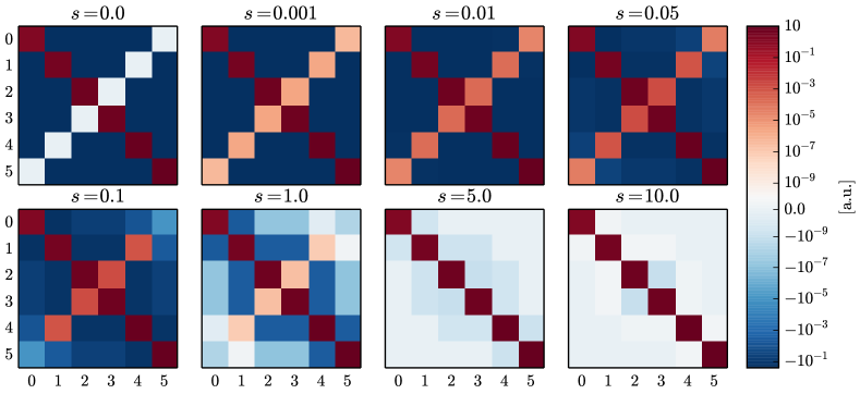
Figure 9.2: SRG evolution of the pairing Hamiltonian with $\delta=1,g=0.5$. The figures show snapshots of the Hamiltonian’s matrix representation at various stages of the flow, indicated by the flow parameters $s$. Note the essentially logarithmic scales of the positive and negative matrix elements, which are bridged by a linear scale in the vicinity of 0.

As a numerical example, we solve the pairing Hamiltonian for $\delta=1.0$ and $g=0.5$. In Fig. 9.2, we show snapshots of the matrix $H(s)$ at different stages of the flow. We can nicely see how the SRG evolution drives the off-diagonal matrix elements to zero. The effect becomes noticeable on our logarithmic color scale around $s=0.05$, where the outermost off-diagonal matrix elements start to lighten. At $s=0.1$, $H_{05}(s)$ has been reduced by four to five orders of magnitude, and at $s=1.0$, essentially all of the off-diagonal matrix elements have been affected to some extent. Note that the strength of the suppression depends on the distance from the diagonal, aside from $H_{05}$ itself, which has a slightly larger absolute value than $H_{04}$ and $H_{15}$. The overall behavior is as expected from our approximate solution (9.50), and the specific deviations can be explained by the approximate nature of that result. Once we have reached $s=10$, the matrix is essentially diagonal, with off-diagonal matrix elements reduced to $10^{-10}$ or less. Only the $2\times 2$ block spanned by the states labeled 2 and 3 has slightly larger off-diagonal matrix elements remaining, which is due to the degeneracy of the corresponding eigenvalues.

Figure 9.3: SRG evolution of the pairing Hamiltonian with $\delta=1,g=0.5$. The left panel shows the diagonal matrix elements $H_{ii}(s)$ as a function of the flow parameter $s$ (dashed lines) and the corresponding eigenvalues (solid lines), the right panel the difference of the two numbers. The color coding is the same in both panels.

In Fig. 9.3, we compare the flowing diagonal matrix elements $H_{ii}(s)$ to the eigenvalues of the pairing Hamiltonian. As we have just mentioned, the pairing Hamiltonian has a doubly degenerate eigenvalue $E_{2}=E_{3}=6\delta-g$, which is why we see only five curves in these plots. For our choice of parameters, the diagonal matrix elements are already in fairly good agreement with the eigenvalues to begin with. Focusing on the right-hand panel of the figure in particular, we see that $H_{00}$ (blue) and $H_{11}$ (red) approach their eigenvalues from above, while $H_{44}$ (orange) and $H_{55}$ (light blue) approach from below as we evolve to large $s$. It is interesting that the diagonal matrix elements are already practically identical to the eigenvalues once we have integrated up to $s=1.0$, despite the non-vanishing off-diagonal matrix elements that are visible in the $s=1.0$ snapshot shown in Fig. 9.2.

9.2.4 Evolution of Nuclear Interactions

Matrix and Operator Flows

In our discussion of the schematic pairing model in the previous section, we have used SRG flows to solve the eigenvalue problem arising from a four-body Schrödinger equation, so we may want to use the same method for the more realistic case of $A$ nucleons interacting by nuclear $NN$, $3N$, etc. interactions (see chapter 8). However, we quickly realize the main problem of such an approach: Working in a full configuration interaction (FCI) picture and assuming even a modest single-particle basis size, e.g., 50 proton and neutron states each, a basis for the description of a nucleus like ${}^{16}\mathrm{O}$ would naively have

$$d(^{16}\mathrm{O})=\begin{pmatrix}50\\ 8\end{pmatrix}\times\begin{pmatrix}50\\ 8\end{pmatrix}\approx 2.88\times 10^{17}$$ (9.51)

configurations, i.e., we would need about 2 exabytes (EB) of memory to store all the coefficients of just one eigenvector (assuming double precision floating-point numbers), and $7\times 10^{17}$ EB to construct the complete Hamiltonian matrix! State-of-the-art methods for large-scale diagonalization are able to reduce the memory requirements and computational effort significantly by exploiting matrix sparseness, and using modern versions of Lanczos-Arnoldi Lanczos:1950sp ; Arnoldi:1951kk or Davidson algorithms Davidson:1989pi , but nuclei in the vicinity of the oxygen isotopic chain are among the heaviest accessible with today’s computational resources (see, e.g., Yang:2013ly ; Barrett:2013oq and references therein). A key feature of Lanczos-Arnoldi and Davidson methods is that the Hamiltonian matrix only appears in the calculation of matrix-vector products. In this way, an explicit construction of the Hamiltonian matrix in the CI basis is avoided, because the matrix-vector product can be calculated from the input $NN$ and $3N$ interactions that only require $\mathscr{O}(n^{4})$ and $\mathscr{O}(n^{6})$ storage, respectively, where $n$ is the size of the single-particle basis (see Sec. 9.3). However, the SRG flow of the previous section clearly forces us to construct and store the Hamiltonian matrix in its entirety — at best, we could save some storage by resizing the matrix once its off-diagonal elements have been sufficiently suppressed.

Instead of trying to evolve the many-body Hamiltonian matrix, we therefore focus on the Hamiltonian operator itself instead. Let us consider a nuclear Hamiltonian with a two-nucleon interaction for simplicity:

$$\hat{H}_{\text{int}}=\hat{T}_{\text{int}}+\hat{V}^{[2]}\,.$$ (9.52)

Since nuclei are self-bound objects, we have to consider the intrinsic form of the kinetic energy,

$$\hat{T}_{\text{int}}\equiv\hat{T}-\hat{T}_{\text{cm}}\,.$$ (9.53)

It is straightforward to show that $\hat{T}_{\text{int}}$ can be written either as a sum of one- and two-body operators,

$$\hat{T}_{\text{int}}=\left(1-\frac{1}{\hat{A}}\right)\sum_{i}\frac{\hat{\mathbf{p}}_{i}^{2}}{2m}-\frac{1}{\hat{A}}\sum_{i<j}\frac{\hat{\mathbf{p}}_{i}\cdot\hat{\mathbf{p}}_{j}}{m}$$ (9.54)

or as a pure two-body operator

$$\hat{T}_{\text{int}}=\frac{2}{\hat{A}}\sum_{i<j}\frac{\hat{\mathbf{q}}_{ij}^{2}}{2\mu}\,,\quad\hat{\mathbf{q}}_{ij}\equiv\hat{\mathbf{p}}_{i}-\hat{\mathbf{p}}_{j}\,.$$ (9.55)

Here, $\hat{A}$ should be treated as a particle-number operator (see Hergert:2009wh ), and $\mu=m/2$ is the reduced nucleon mass (neglecting the proton-neutron mass difference). Using Eq. (9.55) for the present discussion, we can write the intrinsic Hamiltonian as

$$\hat{H}_{\text{int}}=\frac{2}{\hat{A}}\sum_{i<j}\frac{\hat{\mathbf{q}}_{ij}^{2}}{2\mu}+\sum_{i<j}\hat{v}^{[2]}_{ij}\,,$$ (9.56)

and directly consider the evolution of this operator via the flow equation (9.8). It is customary to absorb the flow-parameter dependence completely into the interaction part of the Hamiltonian, and leave the kinetic energy invariant — in our previous examples, this simply amounts to moving the $s-$dependent part of $\hat{H}_{d}(s)$ into $\hat{H}_{od}(s)$. We end up with a flow equation for the two-body interaction:

$$\frac{d{}}{d{s}}v^{[2]}_{ij} =[{\eta},{\hat{v}^{[2]}_{ij}}]\,.$$ (9.57)

In cases where we can expand the two-body interaction in terms of a finite algebra of “basis” operators, Eq. (9.57) becomes a system of ODEs for the expansion coefficients, the so-called running couplings of the Hamiltonian, as explained in earlier chapters of this book. An example is the toy problem discussed in Sec.  9.2.2: We actually expanded our $2\times 2$ in terms of the algebra $\{\hat{I},\hat{\sigma}_{1},\hat{\sigma}_{2},\hat{\sigma}_{3}\}$, and related the matrix elements to the coefficients in this expansion. While the representation of the basis operators of our algebra would force us to use extremely large matrices when we deal with an $A-$body system, we may be able to capture the SRG flow completely with a small set of ODEs for the couplings of the Hamiltonian!

If we cannot identify a set of basis operators for the two-body interaction, we can still resort to representing it as a matrix between two-body states. For a given choice of single-particle basis with size $n$, $\hat{v}^{[2]}$ is then represented by $\mathscr{O}(n^{4})$ matrix elements, as mentioned above. In general, we will then have to face the issue of induced many-body forces, as discussed in Sec.  9.2.4.

SRG in the Two-Nucleon System

Figure 9.4: Repulsive core and tensor force of the Argonne V18 $NN$ interaction Wiringa:1995or in the $(S,T)=(1,0)$ channel. In the left panel, the radial dependencies of the central ($V_{C}(r)$) and tensor components ($V_{T}(r)$) of Argonne V18 are shown, while the right panel shows its momentum space matrix elements in the deuteron partial waves.

Let us now consider the operator flow of the $NN$ interaction in the two-nucleon system, Eq. (9.57). Since the nuclear Hamiltonian is invariant under translations and rotations, it is most convenient to work in momentum and angular momentum eigenstates of the form

$$\,|{q(LS)JMTM_{T}}\rangle\,.$$ (9.58)

Because of the rotational symmetry, the $NN$ interaction conserves the total angular momentum quantum number $J$, and it is easy to show that the total spin $S$ of the nucleon pair is a conserved quantity as well. The orbital angular momentum is indicated by the quantum number $L$, and we remind our readers that $L$ is not conserved, because the nuclear tensor operator

$$S_{ij}(\hat{\mathbf{r}},\hat{\mathbf{r}})=\frac{3}{\hat{\mathbf{r}}^{2}}(\hat{\mathbf{\sigma}}_{i}\cdot\hat{\mathbf{r}})(\hat{\mathbf{\sigma}}_{j}\cdot\hat{\mathbf{r}})-\hat{\mathbf{\sigma}}_{i}\cdot\hat{\mathbf{\sigma}}_{j}$$ (9.59)

can couple states with $\Delta L=\pm 2$. We assume that the interaction is charge-dependent in the isospin channel $T=1$, i.e., matrix elements will depend on the projection $M_{T}=-1,0,1$, which indicates the neutron-neutron, neutron-proton, and proton-proton components of the nuclear Hamiltonian.

In Fig. 9.4 we show features of the central and tensor forces of the Argonne V18 (AV18) interaction Wiringa:1995or in the $(S,T)=(1,0)$ channel, which has the quantum numbers of the deuteron. This interaction belongs to a group of so-called realistic interactions that describe nucleon-nucleon scattering data with high accuracy, but precede the modern chiral forces (see chapter 8, Epelbaum:2009ve ; Machleidt:2011bh ). AV18 is designed to be maximally local in order to be a suitable input for nuclear Quantum Monte Carlo calculations Carlson:2015lq ; Gezerlis:2014zr ; Lynn:2016ec . Because of the required locality, AV18 has a strong repulsive core in the central part of the interaction. Like all $NN$ interactions, it also has a strong tensor force that results from pion exchange. The radial dependencies of these interaction components are shown in the left panel of Fig. 9.4.

When we switch to the momentum representation, we see that the ${}^{3}S_{1}$ partial wave which gives the dominant contribution to the deuteron wave function has strong off-diagonal matrix elements, with tails extending over the entire shown range and as high as $|\hat{\mathbf{q}}|\sim 20\,\,\text{fm}^{-1}$. The matrix elements of the ${}^{3}S_{1}-{}^{3}D_{1}$ mixed partial wave, which are generated exclusively by the tensor force, are sizable as well. The strong coupling between states with low and high relative momenta forces us to use large Hilbert spaces in few- and many-body calculations, even if we are only interested in the lowest eigenstates. Methods like the Lanczos algorithm (see chapter 8 and Lanczos:1950sp ) extract eigenvalues and eigenvectors by repeatedly acting with the Hamiltonian on an arbitrary starting vector in the many-body space, i.e., by repeated matrix-vector products. Even if that vector only has low-momentum or low-energy components in the beginning, an interaction like AV18 will mix in high-momentum components even after a single matrix-vector multiplication, let alone tens or hundreds as in typical many-body calculations. Consequently, the eigenvalues and eigenstates of the nuclear Hamiltonian converge very slowly with respect to the basis size of the Hilbert space (see, e.g., Barrett:2013oq ). To solve this problem, we perform an RG evolution of the $NN$ interaction.

Figure 9.5: Schematic illustration of two types of RG evolution for $NN$ potentials in momentum space: (a) $V_{\text{low-k}}$ running in $\Lambda$, and (b) SRG running in $\lambda$ (see main text). Here, $q$ and $q^{\prime}$ denote the relative momenta of the initial and final state, respectively. At each $\Lambda_{i}$ or $\lambda_{i}$, the matrix elements outside of the corresponding blocks or bands are negligible, implying that high- and low-momentum states are decoupled.

In Fig. 9.5, we show examples for two types of RG evolution that decouple the low- and high-momentum pieces of $NN$ interactions. The first example, Fig. 9.5(a), is a so-called RG decimation, in which the interaction is evolved to decreasing cutoff scales $\Lambda_{0}>\Lambda_{1}>\Lambda_{2}$, and high-momentum modes are “integrated out”. This is the so-called $V_{\text{low-k}}$ approach, which was first used in nuclear physics in the early 2000s Bogner:2003os ; Bogner:2010pq . Note that the resulting low-momentum interaction is entirely confined to states with relative momentum $q\leq\Lambda$. In contrast, Fig. 9.5(b) shows the SRG evolution of the $NN$ interaction to a band-diagonal shape via the flow equation (9.57), using a generator built from the relative kinetic energy in the two-nucleon system Bogner:2007od ; Bogner:2010pq :

$$\eta(\lambda)\equiv[{\frac{\hat{\mathbf{q}}^{2}}{2\mu}},{v(\lambda)}]\,.$$ (9.60)

Instead of the flow parameter $s$, we have parameterized the evolution by $\lambda=s^{-1/4}$, which has the dimensions of a momentum in natural units. Note that the generator (9.60) would vanish if the interaction were diagonal in momentum space. As suggested by Fig.  9.5(b), $\lambda$ is a measure for the “width” of the band in momentum space. Thus, momentum transfers between nucleons are limited according to

$$Q\equiv|\hat{\mathbf{q}}^{\prime}-\hat{\mathbf{q}}|\lesssim\lambda\,,$$ (9.61)

and low- and high-lying momenta are decoupled as $\lambda$ is decreased.

Equation (9.61) implies that the spatial resolution scale of an SRG-evolved interaction (or a $V_{\text{low-k}}$ if we determine the maximum momentum transfer in the low-momentum block) is $\sim 1/Q\geq 1/\lambda$, i.e., only long-ranged components of the $NN$ interaction are resolved explicitly and short-range components of the interaction can just as well be replaced by contact interactions Lepage:1997py ; Bogner:2003os ; Holt:2004ux ; Bogner:2010pq . This is the reason why the realistic $NN$ interactions that accurately describe $NN$ scattering data collapse to a universal long-range interaction when RG-evolved, namely one-pion exchange (OPE). This universal behavior emerges in the range $1.5\,\,\text{fm}^{-1}\leq\lambda\leq 2.5\,\,\text{fm}^{-1}$. Any further evolution to lower $\lambda$ starts to remove pieces of OPE, and eventually generates a pion-less theory that is essentially parameterized in terms of contact interactions. While it is possible to implement such an evolution in the two-body system without introducing pathological behavior Wendt:2011ys , such an interaction must be complemented by strong induced many-nucleon forces once it is applied in finite nuclei, as discussed in Sec. 9.2.4. For this reason, $NN$ interactions are only ever evolved to the aforementioned range of $\lambda$ values.

Nowadays, SRG evolutions are preferred over $V_{\text{low-k}}$ style decimations in nuclear many-body theory, because they can be readily extended to $3N,\ldots$ interactions and to general observables Bogner:2010pq ; Anderson:2010br ; Schuster:2014oq ; More:2015bx ; Jurgenson:2009bs ; Hebeler:2012ly ; Wendt:2013ys . Moreover, we could easily achieve a block decoupling as in Fig. 9.5(a) by using a generator like Anderson:2008hx

$$\eta(\lambda)\equiv[{\underbrace{P_{\Lambda}H(\lambda)P_{\Lambda}+Q_{\Lambda}H(\lambda)Q_{\Lambda}}_{\equiv H_{d}(\lambda)}},{H(\lambda)}]\,.$$ (9.62)

where the projection operators $P_{\Lambda}$ and $Q_{\Lambda}$ partition the relative momentum basis in states with $|\hat{\mathbf{q}}|\leq\Lambda$ and $|\hat{\mathbf{q}}|>\Lambda$, respectively. In this case, $\lambda$ is an auxiliary parameter that is eliminated by evolving $\lambda\to 0$, just like we evolved $s\to\infty$ in Secs. 9.2.2 and 9.2.3.

Implementation of the Flow Equations

We are now ready to implement the flow equations for the $NN$ interaction in the momentum-space partial-wave representation. Using basis states that satisfy the orthogonality and completeness relations

$$\langle{qLSJMTM_{T}}|{q^{\prime}L^{\prime}S^{\prime}J^{\prime}M^{\prime}T^{\prime}M^{\prime}_{T}}\rangle=\frac{\delta(q-q^{\prime})}{qq^{\prime}}\delta_{LL^{\prime}}\delta_{SS^{\prime}}\delta_{JJ^{\prime}}\delta_{MM^{\prime}}\delta_{TT^{\prime}}\delta_{M_{T}M^{\prime}_{T}}$$ (9.63)

and

$$\hat{I}=\sum_{LSJMTM_{T}}\int_{0}^{\infty}dq\,q^{2}\,|{qLSJMTM_{T}}\rangle\bra{qLSJMTM_{T}}\,,$$ (9.64)

respectively, we obtain Bogner:2007od ; Bogner:2010pq

$$\left(-\frac{\lambda^{5}}{4}\right)\frac{d\langle{qL}|\,{\hat{v}}\,|{q^{\prime}L^{\prime}}\rangle}{d\lambda}= -(q^{2}-q^{\prime 2})^{2}\langle{qL}|\,{\hat{v}}\,|{q^{\prime}L^{\prime}}\rangle$$

$$+\sum_{\bar{L}}\int_{0}^{\infty}dpp^{2}\,(q^{2}+q^{\prime}{}^{2}-2p^{2})\langle{qL}|\,{\hat{v}}\,|{p\bar{L}}\rangle\langle{p\bar{L}}|\,{\hat{v}}\,|{q^{\prime}L^{\prime}}\rangle\,,$$ (9.65)

where we have used scattering units ($\hbar^{2}/m=1$) and suppressed the $\lambda$-dependence of $\hat{v}$ as well as the conserved quantum numbers for brevity. Note that a prefactor $-\lambda^{5}/4$ appears due to our change of variables from $s$ to $\lambda$.

We can turn this integro-differential equation back into a matrix flow equation by discretizing the relative momentum variable, e.g., on uniform or Gaussian quadrature meshes. The matrix elements of the relative kinetic energy operator are then simply given by

$$\langle{q_{i}L}|\,{\hat{t}}\,|{q_{j}L^{\prime}}\rangle=q_{i}^{2}\delta_{q_{i}q_{j}}\delta_{LL^{\prime}}\,$$ (9.66)

(with $\hbar^{2}/m=1$). The discretization turns the integration into a simple summation,

$$\int_{0}^{\infty}dq\,q^{2}\;\rightarrow\;\sum_{i}w_{i}q^{2}_{i}\,,$$ (9.67)

where the weights $w_{i}$ depend on our choice of mesh. For a uniform mesh, all weights are identical and correspond to the mesh spacing, while for Gaussian quadrature rules the mesh points and weights have to be determined numerically Press:2007vn . For convenience, we absorb the weights and $q^{2}$ factors from the integral measure into the interaction matrix element,

$$\langle{q_{i}L}|\,{\overline{v}}\,|{q_{j}L^{\prime}}\rangle\equiv\sqrt{w_{i}w_{j}}q_{i}q_{j}\langle{q_{i}L}|\,{\hat{v}}\,|{q_{j}L^{\prime}}\rangle\,.$$ (9.68)

The discretized flow equation can then be written as

$$\frac{d{}}{d{\lambda}}\langle{q_{i}L}|\,{\overline{v}}\,|{q_{j}L^{\prime}}\rangle=-\frac{4}{\lambda^{5}}\langle{q_{i}L}|\,{[{[{\hat{t}},{\overline{v}}]},{\hat{t}+\overline{v}}]}\,|{q_{j}L^{\prime}}\rangle\,.$$ (9.69)

We can solve Eq. (9.69) using a modified version of our Python code for the pairing model, discussed in Sec. 9.2.3. The Python code and sample inputs can be downloaded from https://github.com/ManyBodyPhysics/LectureNotesPhysics/tree/master/Programs/Chapter10-programs/python/srg_nn. Let us briefly discuss the most important modifications.

First, we have a set of functions that read the momentum mesh and the input matrix elements from a file:

⬇

def uniform_weights(momenta):

weights = np.ones_like(momenta)

weights *= abs(momenta[1]-momenta[0])

return weights

def read_mesh(filename):

data = np.loadtxt(filename, comments="#")

dim = data.shape[1]

momenta = data[0,:dim]

return momenta

def read_interaction(filename):

data = np.loadtxt(filename, comments="#")

dim = data.shape[1]

V = data[1:,:dim]

return V

The matrix element files have the following format:

⬇

# momentum space matrix elements

# partial wave J=1, L=0/0, S=1, T=0, MT=0

#

# momentum grid [fm^-1]

0.000000 0.050000 0.100000 0.150000 0.200000 0.250000 0.300000 0.350000 0.400000 0.450000

0.500000 0.550000 0.600000 0.650000 0.700000 0.750000 0.800000 0.850000 0.900000 0.950000

...

6.300000 6.350000 6.400000 6.450000 6.500000 6.550000 6.600000 6.650000 6.700000 6.750000

6.800000 6.850000 6.900000 6.950000 7.000000

#

# matrix elements [MeV fm^3]

-36.94918 -36.83554 -36.49896 -35.95649 -35.23306 -34.35875 -33.36536 -32.28337 -31.13985

-29.95722 -28.75281 -27.53904 -26.32400 -25.11217 -23.90513 -22.70231 -21.50158 -20.29973

...

0.00000 0.00000 0.00000 0.00000 0.00000 0.00000 0.00000 0.00000 0.00000

0.00000 0.00000 0.00000 0.00000 0.00000 0.00000 0.00000 0.00000 0.00000

Comments, indicated by the # character, are ignored. The first set of data is a row containing the mesh points. Here, we have $141$ points in total, ranging from $0$ to $7\,\,\text{fm}^{-1}$ with a spacing of $0.05\,\,\text{fm}^{-1}$. The range of momenta is sufficient for the chiral $NN$ interaction we use in our example, the N³LO potential by Entem and Machleidt with cutoff $\Lambda=500\,\,\text{MeV}$ Entem:2003th ; Machleidt:2011bh , which is considerably softer than the AV18 interaction discussed above. This is followed by a simple $141\times 141$ array of matrix elements. It is straightforward to adapt the format and I/O routines to Gaussian quadrature meshes by including mesh points (i.e., the abscissas) and weights in the data file.

The derivative routine is almost unchanged, save for the prefactor due to the use of $\lambda$ instead of $s$ to parameterize the flow, and the treatment of the kinetic energy operator as explicitly constant:

⬇

def derivative(lam, y, T):

dim = T.shape[0]

# reshape the solution vector into a dim x dim matrix

V = reshape(y, (dim, dim))

# calculate the generator

eta = commutator(T, V)

# dV is the derivative in matrix form

dV = -4.0/(lam**5) * commutator(eta, T+V)

# convert dH into a linear array for the ODE solver

dy = reshape(dV, -1)

return dy

In the main routine of the program, we first set up the mesh and then proceed to read the interaction matrix elements for the different partial waves. We are dealing with a coupled-channel problem because the tensor forces connects partial waves with $\Delta L=2$ in all $S=1$ channels. In our example, we restrict ourselves to the partial waves that contribute to the deuteron bound state, namely ${}^{3}S_{1}$, ${}^{3}D_{1}$, and ${}^{3}S_{1}-{}^{3}D_{1}$. Indicating the orbital angular momenta of these partial waves by indices, we have

$$\mathbf{T}=\begin{pmatrix}\;t\;&\\ &\;t\;\end{pmatrix}\,,\quad\mathbf{V}=\begin{pmatrix}\;\overline{v}_{00}\;&\;\overline{v}_{02}\;\\ \;\overline{v}^{\dagger}_{02}\;&\;\overline{v}_{22}\;\end{pmatrix}\,,$$ (9.70)

where

$$t=\mathrm{diag}\left(q_{0}^{2},\ldots,q_{\text{max}}^{2}\right)\,,$$ (9.71)

since the kinetic energy is independent of $L$. As soon as we pass from the $S-$ into the $D-$ wave in either the rows or the columns, the momentum mesh simply starts from the lowest mesh point again. We use NumPy’s hstack and vstack functions to assemble the interaction matrix from the partial-wave blocks:

⬇

def main():

...

# read individual partial waves

partial_waves=[]

for filename in ["n3lo500_3s1.meq", "n3lo500_3d1.meq", "n3lo500_3sd1.meq"]:

partial_waves.append(read_interaction(filename))

# print partial_waves[-1].shape

# assemble coupled channel matrix

V = np.vstack((np.hstack((partial_waves[0], partial_waves[2])),

np.hstack((np.transpose(partial_waves[2]), partial_waves[1]))

))

# switch to scattering units

V = V/hbarm

...

As discussed earlier, we work in scattering units with $\hbar^{2}/m=1$. Thus, we have to divide the input matrix elements by this factor. We also need to absorb the weights and explicit momentum factors into the interaction matrix. It is convenient to define a conversion matrix for this purpose, which can be multiplied element-wise with the entries of $\mathbf{V}$ using the regular * operator (recall that the matrix product is implemented by the NumPy function dot).

Since we changed variables from $s$ to $\lambda$, we now start the integration at $\lambda=\infty$, or $\lambda\gg 1\,\text{fm}^{-1}$ in practice. As discussed above, we do not evolve all the way to $\lambda=0\,\,\text{fm}^{-1}$, but typically stop before we start integrating out explicit pion physics, e.g., at $\lambda=1.5\,\,\text{fm}^{-1}$. For typical $NN$ interactions, especially those with a hard core like AV18, the flow equations tend to become stiff because they essentially depend on cubic products of the kinetic energy and interaction. For this reason, we use SciPy’s ode class, which provides access to a variety of solvers and greater control over the parameters of the integration process. Specifically, we choose the VODE solver package and its 5th-order Backward Differentiation method Brown:1989wj , which is efficient and works robustly for a large variety of input interactions.

⬇

...

lam_initial = 20.0

lam_final = 1.5

# integrate using scipy.ode instead of scipy.odeint - this gives

# us more control over the solver

solver = ode(derivative,jac=None)

# equations may get stiff, so we use VODE and Backward Differentiation

solver.set_integrator('vode', method='bdf', order=5, nsteps=1000)

solver.set_f_params(T)

solver.set_initial_value(y0, lam_initial)

...

Finally, we reach the loop that integrates the ODE system. We request output from the solver in regular intervals, reducing these intervals as we approach the region of greatest practical interest, $1.5\,\,\text{fm}^{-1}\leq\lambda\leq 2.5\,\,\text{fm}^{-1}$:

⬇

...

while solver.successful() and solver.t > lam_final:

# adjust the step size in different regions of the flow parameter

if solver.t >= 6.0:

ys = solver.integrate(solver.t-1.0)

elif solver.t < 6.0 and solver.t >= 2.5:

ys = solver.integrate(solver.t-0.5)

elif solver.t < 2.5 and solver.t >= lam_final:

ys = solver.integrate(solver.t-0.1)

# add evolved interactions to the list

flowparams.append(solver.t)

Vtmp = reshape(ys,(dim,dim))

Vs.append(Vtmp)

print("%8.5f %14.8f"%(solver.t, eigvalsh((T + Vtmp)*hbarm)[0]))

...

Of course, the ODE solver will typically take several hundred adaptive steps to propagate the solution with the desired accuracy between successive requested values of $\lambda$. At the end of each external step, we diagonalize the evolved Hamiltonian and check whether the lowest eigenvalue, i.e., the deuteron binding energy, remains invariant within the numerical tolerances we use for the ODE solver. To illustrate the evolution of the $NN$ interaction, the code will also generate a sequence of matrix plots at the desired values of $\lambda$, similar to Fig. 9.2 for the pairing Hamiltonian.

Example: Evolution of a Chiral $NN$ Interaction

Figure 9.6: SRG evolution of the chiral N³LO nucleon-nucleon interaction by Entem and Machleidt, with initial cutoff $\Lambda=500\,\,\text{MeV}$ Entem:2003th ; Machleidt:2011bh . In the left column, we show the momentum-space matrix elements of the interaction in the ${}^{3}S_{1}$ partial wave for different values of the SRG resolution scale $\lambda$. The top-most row shows the initial interaction at $s=0\,\,\text{fm}^{4}$ , i.e., “$\lambda=\infty$”. In the right column, we show the $S-$ and $D-$wave components of the deuteron wave function that is obtained by solving the Schrödinger equation with the corresponding SRG-evolved interaction.

As an example of a realistic application, we discuss the SRG evolution of the chiral N³LO nucleon-nucleon interaction by Entem and Machleidt with initial cutoff $\Lambda=500\,\,\text{MeV}$ Entem:2003th ; Machleidt:2011bh . The momentum-space matrix elements of this interaction in the deuteron partial waves are distributed with the Python code discussed in the previous section.

In the top row of Fig. 9.6, we show the matrix elements of the initial interaction in the ${}^{3}S_{1}$ partial wave; the ${}^{3}S_{1}-{}^{3}D_{1}$ and ${}^{3}D_{1}$ are not shown to avoid clutter. Comparing the matrix elements to those of the AV18 interaction we discussed in Sec. 9.2.4, shown in Fig. 9.4, we note that the chiral interaction has much weaker off-diagonal matrix elements to begin with. While the AV18 matrix elements extend as high as $|\hat{\mathbf{q}}|\sim 20\,\,\text{fm}^{-1}$, the chiral interaction has no appreciable strength in states with $|\hat{\mathbf{q}}|\sim 4.5\,\,\text{fm}^{-1}$. In nuclear physics jargon, AV18 is a much harder interaction than the chiral interaction because of the former’s strongly repulsive core. By evolving the initial interaction to $3\,\,\text{fm}^{-1}$ and then to $2\,\,\text{fm}^{-1}$, the offdiagonal matrix elements are suppressed, and the interaction is almost entirely contained in a block of states with $|\hat{\mathbf{q}}|\sim 2\,\,\text{fm}^{-1}$, except for a weak diagonal ridge.

Next to the matrix elements, we also show the deuteron wave functions that we obtain by solving the Schrödinger equation with the initial and SRG-evolved chiral interactions. For the unevolved $NN$ interaction, the $S-$wave ($L=0$) component of the wave function is suppressed at small relative distances, which reflects short-range correlations between the nucleons. (For AV18, the $S-$wave component of the deuteron wave function vanishes at $r=0\,\,\text{fm}$ due to the hard core.) There is also a significant $D-$wave ($L=2$) admixture due to the tensor interaction. As we lower the resolution scale, the “correlation hole” in the wave function is filled in, and all but eliminated once we reach $\lambda=2.0\,\,\text{fm}^{-1}$. The $D-$wave admixture is reduced significantly, as well, because the evolution suppresses the matrix elements in the ${}^{3}S_{1}-{}^{3}D_{1}$ wave, which are responsible for this mixing Bogner:2010pq . Focusing just on the $S-$wave, the wave function is extremely simple and matches what we would expect for two almost independent, uncorrelated nucleons. The Pauli principle does not affect the coordinate-space part of the wave function here because the overall antisymmetry of the deuteron wave function is ensured by its spin and isospin parts.

Let us dwell on the removal of short-range correlations from the wave function for another moment, and consider the exact eigenstates of the initial $NN$ Hamiltonian,

$$\hat{H}(0)\,|{\psi_{n}}\rangle=E_{n}\,|{\psi_{n}}\rangle\,.$$ (9.72)

The eigenvalues are invariant under a unitary transformation, e.g., an SRG evolution,

$$\hat{H}(\lambda)\hat{U}(\lambda)\,|{\psi_{n}}\rangle\equiv\hat{U}(\lambda)\hat{H}(0)\hat{U}^{\dagger}(\lambda)\hat{U}(\lambda)\,|{\psi_{n}}\rangle=E_{n}\hat{U}(\lambda)\,|{\psi_{n}}\rangle\,.$$ (9.73)

We can interpret this equation as a shift of correlations from the wave function into the effective, RG-improved Hamiltonian. When we solve the Schrödinger equation numerically, we can usually only obtain an approximation $\,|{\phi_{n}}\rangle$ of the exact eigenstate. In the ideal case, this is merely due to finite-precision arithmetic on a computer, but more often, we also have systematic approximations, e.g., mesh discretizations, finite basis sizes, many-body truncations (think of the cluster operator in Coupled Cluster, for instance, cf.  chapter 8), etc. If we use the evolved Hamiltonian $\hat{H}(\lambda)$, we only need to approximate the transformed eigenstate,

$$\,|{\phi_{n}}\rangle\approx\hat{U}(\lambda)\,|{\psi_{n}}\rangle\,$$ (9.74)

instead of $\,|{\psi_{n}}\rangle$, which is often a less demanding task. This is certainly true for our deuteron example at $\lambda=2.0\,\,\text{fm}^{-1}$, where we no longer have to worry about short-range correlations.

Induced Interactions

As discussed earlier in this section, our motivation for using the SRG to decouple the low- and high-lying momentum components of $NN$ interactions is to improve the convergence of many-body calculations. The decoupling prevents the Hamiltonian from scattering nucleon pairs from low to high momenta or energies, which in turn allows configuration-space based methods to achieve convergence in much smaller Hilbert spaces than for a “bare”, unevolved interaction. This makes it possible to extend the reach of these methods to heavier nuclei Roth:2011kx ; Barrett:2013oq ; Jurgenson:2013fk ; Roth:2014fk ; Hergert:2013ij ; Hergert:2013mi ; Hergert:2014vn ; Hergert:2016jk ; Hagen:2010uq ; Roth:2012qf ; Binder:2013zr ; Binder:2014fk ; Soma:2011vn ; Soma:2013ys ; Soma:2014fu ; Soma:2014eu .

In practical applications, we pay a price for the improved convergence. To illustrate the issue, we consider the Hamiltonian in a second-quantized form, assuming only a two-nucleon interaction for simplicity (cf. Eq. (9.56)):

$$\hat{H}_{\text{int}}=\frac{1}{4}\sum_{pqrs}\langle{pq}|\,{\frac{\hat{\mathbf{q}}^{2}}{2\mu}+\hat{v}}\,|{rs}\rangle a^{\dagger}_{p}a^{\dagger}_{q}a_{s}a_{r}\,.$$ (9.75)

If we plug the kinetic energy and interaction into the commutators in Eqs. (9.60) and (9.8), we obtain

$$[{a^{\dagger}_{i}a^{\dagger}_{j}a_{l}a_{k}},{a^{\dagger}_{p}a^{\dagger}_{q}a_{s}a_{r}}]=\delta_{lp}a^{\dagger}_{i}a^{\dagger}_{j}a^{\dagger}_{q}a_{s}a_{r}a_{k}+a^{\dagger}a^{\dagger}a^{\dagger}aaa-\delta_{lp}\delta_{kq}a^{\dagger}_{i}a^{\dagger}_{j}a_{s}a_{r}+a^{\dagger}a^{\dagger}aa\,,$$ (9.76)

where the terms with suppressed indices schematically stand for additional two- and three-body operators. Even if we start from a pure $NN$ interaction, the SRG flow will induce operators of higher rank, i.e., $3N$, $4N$, and in general up to $A$-nucleon interactions. Of course, these induced interactions are only probed if we study an $A$-nucleon system. If we truncate the SRG flow equations at the two-body level, the properties of the two-nucleon system are preserved, in particular the $NN$ scattering phase shifts and the deuteron binding energy. A truncation at the three-body level ensures the invariance of observables in $A=3$ nuclei, e.g. ${}^{3}\mathrm{H}$ and ${}^{3}\mathrm{He}$ ground-state energies, and so on.

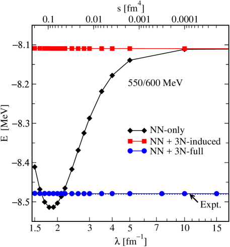
Figure 9.7: Ground state energy of ${}^{3}\mathrm{H}$ as a function of the flow parameter $\lambda$ for chiral NNLO $NN$ and $NN\!+\!3N$ interactions (see Hebeler:2012ly for details). $NN$-only means initial and induced $3N$ interactions are discarded, $NN\!+\!3N$-induced takes only induced $3N$ interactions into account, and $3N$-full contains initial $3N$ interactions as well. The black dotted line shows the experimental binding energy Wang:2012uq . Data for the figure courtesy of K. Hebeler.

Nowadays, state-of-the-art SRG evolutions of nuclear interactions are performed in the three-body system Jurgenson:2009bs ; Jurgenson:2011zr ; Jurgenson:2013fk ; Hebeler:2012ly ; Wendt:2013uq . In Fig. 9.7, we show ${}^{3}\mathrm{H}$ ground-state energies that have been calculated with a family of SRG-evolved interactions that is generated from a chiral NNLO $NN$ interaction by Epelbaum, Glöckle, and Meißner Epelbaum:2002nr ; Epelbaum:2006mo , and a matching $3N$ interaction (see Hebeler:2012ly for full details). As mentioned above, the SRG evolution is not unitary in the three-body system if we truncate the evolved interaction and the SRG generator at the two-body level (N$N$-only). The depends strongly on $\lambda$, varying by 5–6% over the typical range that we consider here (cf. Sec. 9.2.4). If we truncate the operators at the three-body level instead, induced $3N$ interactions are properly included and the unitarity of the transformation is restored ($NN\!+\!3N$-induced): The energy does not change as $\lambda$ is varied. Finally, the curve $NN\!+\!3N$-full shows results of calculations in which a $3N$ force was included in the initial Hamiltonian and evolved consistently to lower resolution scale as well. Naturally, the triton ground-state energy is invariant under the SRG flow, and it closely reproduces the experimental value because the $3N$ interaction’s low-energy constants are usually fit to give the correct experimental ${}^{3}\mathrm{H}$ ground-state energy (see, e.g., Epelbaum:2009ve ; Machleidt:2011bh ; Gazit:2009qf ).

Our example shows that it is important to track induced interactions, especially when we want to use evolved nuclear Hamiltonians beyond the few-body systems we have focused on here. The nature of the SRG as a continuous evolution works at least somewhat in our favor: As discussed above, truncations of the SRG flow equations lead to a violation of unitarity that manifests as a (residual) dependence of our calculated few- and many-body observables on the resolution scale $\lambda$. We can use this dependence as a tool to assess the size of missing contributions, although one has to take great care to disentangle them from the effects of many-body truncations, unless one uses quasi-exact methods like the NCSM (see, e.g., Bogner:2010pq ; Jurgenson:2009bs ; Hebeler:2012ly ; Roth:2011kx ; Hergert:2013mi ; Hergert:2013ij ; Binder:2014fk ; Soma:2014eu ; Griesshammer:2015dp ). If we want more detailed information, then we cannot avoid to work with $3N,4N,\ldots$ or higher many-nucleon forces. The empirical observation that SRG evolutions down to $\lambda\sim 1.5\,\text{fm}^{-1}$ appear to preserve the natural hierarchy of nuclear forces, i.e., $NN>3N>4N>\ldots$, suggests that we can truncate induced forces whose contributions would be smaller than the desired accuracy of our calculations.

While we may not have to go all the way to the treatment of induced $A-$nucleon operators, which would be as expensive as implementing the matrix flow in the $A-$body system (cf. Sec. 9.2.4), dealing with induced $3N$ operators is already computationally expensive enough. Treating induced $4N$ forces explicitly is out of the question, except in schematic cases. However, there is a way of accounting for effects of induced $3N,\ldots$ forces in an implicit manner, by performing SRG evolutions in the nuclear medium.

9.3 The In-Medium SRG

As discussed in the previous section, we now want to carry out the operator evolution (9.8) in the nuclear medium. The idea is to decompose a given $N$-body operator into in-medium contributions of lower rank and residual components that can be truncated safely. To this end, we first have to lay the groundwork by reviewing the essential elements of normal ordering, as well as Wick’s theorem.

9.3.1 Normal Ordering and Wick’s Theorem

Normal-Ordered Operators

To construct normal-ordered operators, we start from the usual Fermionic creation and annihilation operators, $a^{\dagger}_{i}$ and $a_{i}$, which satisfy the canonical anticommutation relations

$$\big{\{}{a^{\dagger}_{i}},{a^{\dagger}_{j}}\big{\}}=\big{\{}{a_{i}},{a_{j}}\big{\}}=0\,,\quad\big{\{}{a^{\dagger}_{i}},{a_{j}}\big{\}}=\delta_{ij}\,.$$ (9.77)

The indices are collective labels for the quantum numbers of our single-particle states. Using the creators and annihilators, we can express any given $A$-body operator in second quantization. Moreover, we can construct a complete basis for a many-body Hilbert space by acting with products of $a^{\dagger}_{i}$ on the particle vacuum,

$$\,|{\Phi\{i_{1}\ldots i_{A}\}}\rangle=\prod_{k=1}^{A}a^{\dagger}_{i_{k}}\,|{\text{vac}}\rangle\,,$$ (9.78)

and letting the indices $i_{1},\ldots,i_{A}$ run over all single-particle states. The states $\,|{\Phi\{i_{1}\ldots i_{A}\}}\rangle$ are, of course, nothing but antisymmetrized product states, i.e., Slater determinants.

Of course, not all of the Slater determinants in our basis are created equal. We can usually find a Slater determinant that is a fair approximation to the nuclear ground state, and use it as a reference state for the construction and organization of our many-body basis. By simple energetics, the ground state and low-lying excitation spectrum of an $A$-body nucleus are usually dominated by excitations of particles in the vicinity of the reference state’s Fermi energy. This is especially true for $NN$ interactions that have been evolved to a low resolution scale $\lambda$ (see Sec.  9.2.4). For such forces, the coupling between basis states whose energy expectation values differ by much more than the characteristic energy $\hbar^{2}\lambda^{2}/m$ is suppressed.

Slater determinants that are variationally optimized through a Hartree-Fock (HF) calculation have proven to be reasonable reference states for interactions with $\lambda\approx 2.0\,\text{fm}^{-1}$ (see, e.g., Refs. Bogner:2010pq ; Roth:2010vp ; Barrett:2013oq ; Hagen:2014ve ; Hergert:2016jk ; Tichai:2016vl and references therein), allowing post-HF methods like MBPT, CC, or the IMSRG discussed below to converge rapidly to the exact result. Starting from such a HF reference state $\,|{\Phi}\rangle$, we can obtain a basis consisting of the state itself and up to $A$-particle, $A$-hole ($ApAh$) excitations:

$$\,|{\Phi}\rangle,\,a^{\dagger}_{p_{1}}a_{h_{1}}\,|{\Phi}\rangle,\;\ldots\;,\,a^{\dagger}_{p_{1}}\ldots a^{\dagger}_{p_{A}}a_{h_{A}}\ldots a_{h_{1}}\,|{\Phi}\rangle\,.$$ (9.79)

Here, indices $p_{i}$ and $h_{i}$ run over all one-body basis states with energies above (particle states) and below the Fermi level (hole states), respectively. Such bases work best for systems with large gaps in the single-particle spectrum, e.g., closed-shell nuclei. If the gap is small, excited basis states can be nearly degenerate with the reference state, which usually results in spontaneous symmetry breaking and strong configuration mixing.

We can now introduce a one-body operator that is normal-ordered with respect to the reference state $\,|{\Phi}\rangle$ by defining

$$a^{\dagger}_{i}a_{j}\equiv\big{\{}a^{\dagger}_{i}a_{j}\big{\}}+\,\contraction[1.5ex]{}{a}{{}^{\dagger}_{i}}{a}a^{\dagger}_{i}a_{j}\,,$$ (9.80)

where the brackets $\{\ldots\}$ indicate normal ordering, and the brace over a pair of creation and annihilation operators means that they have been contracted. The contraction itself is merely the expectation value of the operator in the reference state $\,|{\Phi}\rangle$:

$$\contraction[1.5ex]{}{a}{{}^{\dagger}_{i}}{a}a^{\dagger}_{i}a_{j}\equiv\langle{\Phi}|\,{a^{\dagger}_{i}a_{j}}\,|{\Phi}\rangle\equiv\rho_{ji}\,.$$ (9.81)

By definition, the contractions are identical to the elements of the one-body density matrix of $\,|{\Phi}\rangle$ Ring:1980bb . Starting from the one-body case, we can define normal-ordered $A$-body operators recursively by evaluating all contractions between creation and annihilation operators, e.g.,

$$a^{\dagger}_{i_{1}}\ldots a^{\dagger}_{i_{A}}a_{j_{A}}\ldots a_{j_{1}}$$

$$\equiv\,\big{\{}a^{\dagger}_{i_{1}}\ldots a^{\dagger}_{i_{A}}a_{j_{A}}\ldots a_{j_{1}}\big{\}}$$

$$\hphantom{\equiv}+\contraction[1.5ex]{}{a}{{}^{\dagger}_{i_{1}}}{a}a^{\dagger}_{i_{1}}a_{j_{1}}\big{\{}a^{\dagger}_{i_{2}}\ldots a^{\dagger}_{i_{A}}a_{j_{A}}\ldots a_{j_{2}}\big{\}}-\;\contraction[1.5ex]{}{a}{{}^{\dagger}_{i_{1}}}{a}a^{\dagger}_{i_{1}}a_{j_{2}}\big{\{}a^{\dagger}_{i_{2}}\ldots a^{\dagger}_{i_{A}}a_{j_{A}}\ldots a_{j_{3}}a_{j_{1}}\big{\}}+\text{\,singles}$$

$$\hphantom{\equiv}+\left(\contraction[1.5ex]{}{a}{{}^{\dagger}_{i_{1}}}{a}a^{\dagger}_{i_{1}}a_{j_{1}}\contraction[1.5ex]{}{a}{{}^{\dagger}_{i_{1}}}{a}a^{\dagger}_{i_{2}}a_{j_{2}}-\contraction[1.5ex]{}{a}{{}^{\dagger}_{i_{1}}}{a}a^{\dagger}_{i_{1}}a_{j_{2}}\contraction[1.5ex]{}{a}{{}^{\dagger}_{i_{1}}}{a}a^{\dagger}_{i_{2}}a_{j_{1}}\right)\big{\{}a^{\dagger}_{i_{3}}\ldots a^{\dagger}_{i_{A}}a_{j_{A}}\ldots a_{j_{3}}\big{\}}+\text{\,doubles}$$

$$\hphantom{\equiv}+\,\ldots\,+\text{\,full contractions}\,.$$ (9.82)

Here, we have followed established quantum chemistry jargon (singles, doubles, etc.) for the number of contractions in a term (cf. chapter 8). Note that the double contraction shown in the next-to-last line is identical to the factorization formula for the two-body density matrix of a Slater determinant,

$$\rho_{j_{1}j_{2}i_{1}i_{2}}\equiv\langle{\Phi}|\,{a^{\dagger}_{i_{1}}a^{\dagger}_{i_{2}}a_{j_{2}}a_{j_{1}}}\,|{\Phi}\rangle=\rho_{i_{1}j_{1}}\rho_{i_{2}j_{2}}-\rho_{i_{1}j_{2}}\rho_{i_{2}j_{1}}\,.$$ (9.83)

From Eq. (9.80), it is evident that $\langle{\Phi}|\,{\big{\{}a^{\dagger}_{i}a_{j}\big{\}}}\,|{\Phi}\rangle$ must vanish, and this is readily generalized to expectation values of arbitrary normal-ordered operators in the reference state $\,|{\Phi}\rangle$,

$$\langle{\Phi}|\,{\big{\{}a^{\dagger}_{i_{1}}\ldots a_{i_{1}}\big{\}}}\,|{\Phi}\rangle=0\,.$$ (9.84)

This property of normal-ordered operators greatly facilitates calculations that require the evaluation of matrix elements in a space spanned by excitations of $\,|{\Phi}\rangle$. Another important property is that we can freely anticommute creation and annihilation operators within a normal-ordered string (see problem 9.6):

$$\big{\{}\ldots a^{\dagger}_{i}a_{j}\ldots\big{\}}=-\big{\{}\ldots a_{j}a^{\dagger}_{i}\ldots\big{\}}\,.$$ (9.85)

As an example, we consider an intrinsic nuclear $A$-body Hamiltonian containing both $NN$ and $3N$ interactions,

$$H=\left(1-\frac{1}{\hat{A}}\right)\hat{T}^{[1]}+\frac{1}{\hat{A}}\hat{T}^{[2]}+\hat{V}^{[2]}+\hat{V}^{[3]}\,,$$ (9.86)

where the one- and two-body kinetic energy terms are

$$\hat{T}^{[1]} \equiv\sum\frac{\hat{\mathbf{p}}^{2}_{i}}{2m}\,,$$ (9.87)

$$\hat{T}^{[2]} \equiv-\frac{1}{m}\sum_{i<j}\hat{\mathbf{p}}_{i}\cdot\hat{\mathbf{p}}_{j}$$ (9.88)

(see Sec. 9.2.4 and Hergert:2009wh ). Choosing a single Slater determinant $\,|{\Phi}\rangle$ as the reference state, we can rewrite the Hamiltonian exactly in terms of normal-ordered operators,

$$\hat{H} =E+\sum_{ij}f_{ij}\big{\{}a^{\dagger}_{i}a_{j}\big{\}}+\frac{1}{4}\sum_{ijkl}\Gamma_{ijkl}\big{\{}a^{\dagger}_{i}a^{\dagger}_{j}a_{l}a_{k}\big{\}}+\frac{1}{36}\sum_{ijklmn}W_{ijklmn}\big{\{}a^{\dagger}_{i}a^{\dagger}_{j}a^{\dagger}_{k}a_{n}a_{m}a_{l}\big{\}}\,,$$ (9.89)

where the labels for the individual contributions have been chosen for historical reasons. For convenience, we will work in the eigenbasis of the one-body density matrix in the following, so that

$$\rho_{ab}=n_{a}\delta_{ab}\,,\quad n_{a}\in\{0,1\}\,.$$ (9.90)

The individual normal-ordered contributions in Eq. (9.89) are then given by

$$E =\left(1-\frac{1}{A}\right)\sum_{a}\langle{a}|\,{\hat{t}^{[1]}}\,|{a}\rangle n_{a}+\frac{1}{2}\sum_{ab}\langle{ab}|\,{\frac{1}{A}\hat{t}^{[2]}\!+\!\hat{v}^{[2]}}\,|{ab}\rangle n_{a}n_{b}+\frac{1}{6}\sum_{abc}\langle{abc}|\,{\hat{v}^{[3]}}\,|{abc}\rangle n_{a}n_{b}n_{c}\,,$$ (9.91)

$$f_{ij} =\left(1-\frac{1}{A}\right)\langle{i}|\,{\hat{t}^{[1]}}\,|{j}\rangle+\sum_{a}\langle{ia}|\,{\frac{1}{A}\hat{t}^{[2]}\!+\!\hat{v}^{[2]}}\,|{ja}\rangle n_{a}+\frac{1}{2}\sum_{ab}\langle{iab}|\,{\hat{v}^{[3]}}\,|{jab}\rangle n_{a}n_{b}\,,$$ (9.92)

$$\Gamma_{ijkl} =\langle{ij}|\,{\frac{1}{A}\hat{t}^{(2)}\!+\!\hat{v}^{[2]}}\,|{kl}\rangle+\sum_{a}\langle{ija}|\,{\hat{v}^{[3]}}\,|{kla}\rangle n_{a}\,,$$ (9.93)

$$W_{ijklmn} =\langle{ijk}|\,{\hat{v}^{[3]}}\,|{lmn}\rangle\,.$$ (9.94)

Due to the occupation number factors in Eqs. (9.91)–(9.93), the sums run only over states that are occupied in the reference state. This means that the zero-, one-, and two-body parts of the Hamiltonian all contain in-medium contributions from the free-space 3N interaction.

For low-momentum interactions, it has been shown empirically that the omission of the normal-ordered three-body piece of the Hamiltonian causes a deviation of merely 1–2% in ground-state and (absolute) excited state energies of light and medium-mass nuclei Hagen:2007zc ; Roth:2011kx ; Roth:2012qf ; Binder:2013fk ; Gebrerufael:2016fe . This normal-ordered two-body approximation (NO2B) to the Hamiltonian is useful for practical calculations, because it provides an efficient means to account for $3N$ force effects in nuclear many-body calculations without incurring the computational expense of explicitly treating three-body operators. In Sec.  9.3.2, we will see that the NO2B approximation also meshes in a natural way with the framework of the IMSRG, which makes it especially appealing for our purposes.

Wick’s Theorem

The normal-ordering formalism has additional benefits for the evaluation of products of normal-ordered operators. Wick’s theorem (see, e.g., Shavitt:2009 ), which is a direct consequence of Eq. (9.3.1), allows us to expand such products in the following way:

$$\big{\{}a^{\dagger}_{i_{1}}\ldots a^{\dagger}_{i_{N}}a_{j_{N}}\ldots a_{j_{1}}\big{\}}\big{\{}a^{\dagger}_{k_{1}}\ldots a^{\dagger}_{k_{M}}a_{l_{M}}\ldots a_{l_{1}}\big{\}}$$

$$=(-1)^{M\cdot N}\big{\{}a^{\dagger}_{i_{1}}\ldots a^{\dagger}_{i_{N}}a^{\dagger}_{k_{1}}\ldots a^{\dagger}_{k_{M}}a_{j_{N}}\ldots a_{j_{1}}a_{l_{M}}\ldots a_{l_{1}}\big{\}}$$

$$\hphantom{=}+(-1)^{M\cdot N}\contraction[1.5ex]{}{a}{{}^{\dagger}_{i_{1}}}{a}a^{\dagger}_{i_{1}}a_{l_{1}}\big{\{}a^{\dagger}_{i_{2}}\ldots a^{\dagger}_{k_{M}}a_{j_{N}}\ldots a_{l_{2}}\big{\}}$$

$$\hphantom{\equiv}+(-1)^{(M-1)(N-1)}\contraction[1.5ex]{}{a}{{}^{\dagger}_{j_{N}}}{a}a_{j_{N}}a^{\dagger}_{k_{1}}\big{\{}a^{\dagger}_{i_{1}}\ldots a^{\dagger}_{k_{M}}a_{j_{N}}\ldots a_{j_{2}}\big{\}}$$

$$\hphantom{=}+\text{\,singles}+\text{\,doubles}+\ldots\,.$$ (9.95)

The phase factors appear because we anti-commute the creators and annihilators until they are grouped in the canonical order, i.e., all $a^{\dagger}$ appear to the left of the $a$. In the process, we also encounter a new type of contraction,

$$\contraction[1.5ex]{}{a}{{}^{\dagger}_{i}}{a}a_{i}a^{\dagger}_{j}\equiv\langle{\Phi}|\,{a_{i}a^{\dagger}_{j}}\,|{\Phi}\rangle=\delta_{ij}-\rho_{ij}\equiv\overline{\rho}_{ij}\,,$$ (9.96)

as expected from the canonical anti-commutator algebra. $\overline{\rho}$ is the so-called hole density matrix.

The defining feature of Eq. (9.3.1) is that only contractions between one index from each of the two strings of creation and annihilation operators appear in the expansion, because contractions between indices within a single operator string have already been subtracted when we normal ordered it initially. In practical calculations, this leads to a substantial reduction of terms. An immediate consequence of Eq. (9.3.1) is that a product of normal-ordered $M$ and $N$-body operators has the general form

$$\hat{A}^{[M]}\hat{B}^{[N]}=\sum_{k=|M-N|}^{M+N}\hat{C}^{[k]}\,.$$ (9.97)

Note that zero-body contributions, i.e., plain numbers, can only be generated if both operators have the same particle rank.

9.3.2 In-Medium SRG Flow Equations

Induced Forces Revisited

In Sec. 9.2.4, we discussed how SRG evolutions naturally induce $3N$ and higher many-nucleon forces, because every evaluation of the commutator on the right-hand side of the operator flow equation (9.8) increases the particle rank of $\hat{H}(s)$, e.g.,

$$\sum_{ijklpqrs}\eta_{ijkl}H_{pqrs}[{a^{\dagger}_{i}a^{\dagger}_{j}a_{l}a_{k}},{a^{\dagger}_{p}a^{\dagger}_{q}a_{s}a_{r}}]=-\sum_{ijkqrs}\eta_{ijkl}H_{kqrs}a^{\dagger}_{i}a^{\dagger}_{j}a^{\dagger}_{q}a_{s}a_{r}a_{l}+\text{3N terms}+\text{2N terms}\,.$$ (9.98)

Note that there are no induced $4N$ interactions, and that commutators involving at least one one-body operator do not change the particle rank (see problem 9.6). In the free-space evolution, we found that the truncation of $3N$ forces in the flowing Hamiltonian caused a significant flow-parameter dependence of observables in $A\geq 3$ systems.

Working in the medium and using normal-ordered operators, we can expand the induced $3N$ operators:

$$\sum_{ijkqrs}\eta_{ijkl}H_{kqrs}a^{\dagger}_{i}a^{\dagger}_{j}a^{\dagger}_{q}a_{s}a_{r}a_{l}=\sum_{ijkqrs}\eta_{ijkl}H_{kqrs}\Big{(} \big{\{}a^{\dagger}_{i}a^{\dagger}_{j}a^{\dagger}_{q}a_{s}a_{r}a_{l}\big{\}}+n_{q}\delta_{qs}\big{\{}a^{\dagger}_{i}a^{\dagger}_{j}a_{r}a_{l}\big{\}}+n_{j}n_{q}\delta_{jr}\delta_{qs}\big{\{}a^{\dagger}_{i}a_{l}\big{\}}$$

$$+n_{i}n_{j}n_{q}\delta_{il}\delta_{jr}\delta_{qs}+\text{permutations}\Big{)}\,.$$ (9.99)

If we now truncate operators to the normal-ordered two-body level, we keep all the in-medium contributions of the induced $3N$ terms, and retain information that we would have lost in the free-space evolution. These in-medium contributions continuously feed into the 0B, 1B, and 2B matrix elements of the flowing Hamiltonian as we integrate Eq. (9.8).

The IMSRG(2) Scheme

The evolution of the Hamiltonian or any other observable by means of the flow equation (9.8) is a continuous unitary transformation in $A-$nucleon space only if we keep up to induced $A$-nucleon forces. Because an explicit treatment of induced contributions up to the $A$-body level is simply not feasible, we have to introduce a truncation to close the system of flow equations.

As explained in the previous subsection, we can make such truncations more robust if we normal order all operators with respect to a reference state that is a fair approximation to the ground state of our system (or another exact eigenstate we might want to target). Here, we choose to truncate operators at the two-body level, to avoid the computational expense of treating explicit three-body operators. For low-momentum $NN+3N$ Hamiltonians, the empirical success of the NO2B approximation mentioned at the end of Sec. 9.3.1 seems to support this truncation: The omission of the normal-ordered $3N$ term in exact calculations causes deviations of only $\sim 1\%$ in the oxygen, calcium, and nickel isotopes Roth:2012qf ; Binder:2013fk ; Binder:2014fk .

Following this line of reasoning, we demand that for all values of the flow parameter $s$

$$\hat{\eta}(s) \approx\hat{\eta}^{(1)}(s)+\hat{\eta}^{(2)}(s)\,,$$ (9.100)

$$\hat{H}(s) \approx E(s)+f(s)+\Gamma(s)\,,$$ (9.101)

$$\frac{d{}}{d{s}}\hat{H}(s) \approx\frac{d{}}{d{s}}E(s)+\frac{d{}}{d{s}}f(s)+\frac{d{}}{d{s}}\Gamma(s)\,.$$ (9.102)

This is the so-called IMSRG(2) truncation, which has been our primary workhorse in past applications Tsukiyama:2011uq ; Tsukiyama:2012fk ; Hergert:2013mi ; Hergert:2013ij ; Hergert:2014vn ; Morris:2015ve ; Hergert:2016jk . It is the basis for all results that we will discuss in the remainder of this chapter. The IMSRG(2) is a cousin to Coupled Cluster with Singles and Doubles (CCSD) and the ADC(3) scheme in Self-Consistent Green’s Function Theory (see chapters 8 and 11). Since all three methods (roughly) aim to describe the same type and level of many-body correlations, we expect to obtain similar results for observables.

Let us introduce the permutation symbol $P_{ij}$ to interchange the indices of any expression, i.e.,

$$P_{ij}g(\ldots,i,\ldots,j)\equiv g(\ldots,j,\ldots,i)\,,$$ (9.103)

Plugging equations (9.100)–(9.102) into the operator flow equation (9.8) and evaluating the commutators with the expressions from the appendix, we obtain the following system of IMSRG(2) flow equations:

$$\frac{d{E}}{d{s}} =\sum_{ab}(n_{a}-n_{b})\eta_{ab}f_{ba}+\frac{1}{2}\sum_{abcd}\eta_{abcd}\Gamma_{cdab}n_{a}n_{b}\bar{n}_{c}\bar{n}_{d}\,,$$ (9.104)

$$\frac{d{f_{ij}}}{d{s}} =\sum_{a}(1+P_{ij})\eta_{ia}f_{aj}+\sum_{ab}(n_{a}-n_{b})(\eta_{ab}\Gamma_{biaj}-f_{ab}\eta_{biaj})$$

$$\quad+\frac{1}{2}\sum_{abc}(n_{a}n_{b}\bar{n}_{c}+\bar{n}_{a}\bar{n}_{b}n_{c})(1+P_{ij})\eta_{ciab}\Gamma_{abcj}\,,$$ (9.105)

$$\frac{d{\Gamma_{ijkl}}}{d{s}} =\sum_{a}\left\{(1-P_{ij})(\eta_{ia}\Gamma_{ajkl}-f_{ia}\eta_{ajkl})-(1-P_{kl})(\eta_{ak}\Gamma_{ijal}-f_{ak}\eta_{ijal})\right\}$$

$$\quad+\frac{1}{2}\sum_{ab}(1-n_{a}-n_{b})(\eta_{ijab}\Gamma_{abkl}-\Gamma_{ijab}\eta_{abkl})$$

$$\quad+\sum_{ab}(n_{a}-n_{b})(1-P_{ij})(1-P_{kl})\eta_{aibk}\Gamma_{bjal}\,.$$ (9.106)

Here, $\bar{n}_{i}=1-n_{i}$, and the $s$-dependence has been suppressed for brevity. To obtain ground-state energies, we integrate Eqs. (9.104)–(9.106) from $s=0$ to $s\to\infty$, starting from the initial components of the normal-ordered Hamiltonian (Eqs. (9.91)–(9.93)) (see Secs. 9.3.6 and 9.3.7 for numerical examples).

By integrating the flow equations, we absorb many-body correlations into the flowing normal-ordered Hamiltonian, summing certain classes of terms in the many-body expansion to all orders Hergert:2016jk . We can identify specific structures by looking at the occupation-number dependence of the terms in Eqs. (9.104)–(9.106): for instance, $\bar{n}_{i}$ and $n_{i}$ restrict summations to particle and hole states, respectively (cf. equation (9.90)). Typical IMSRG generators (see Sec. 9.3.4) are proportional to the (offdiagonal) Hamiltonian, which means that the two terms in the zero-body flow equation essentially have the structure of second-order energy corrections, but evaluated for the flowing Hamiltonian $\hat{H}(s)$. Thus, we can express the equation in terms of Hugenholtz diagrams as

$$\frac{d{}}{d{s}}E=\vbox{\hbox{ \begin{picture}(0.7,1.0)\put(0.0,0.0){\includegraphics[height=52.03227pt]{fig/imsrg_0bflow_1b.pdf}} \end{picture} }}+\vbox{\hbox{ \begin{picture}(0.7,1.0)\put(0.0,0.0){\includegraphics[height=52.03227pt]{fig/imsrg_0bflow_2b.pdf}} \end{picture} }}\,.$$ (9.107)

Note that the energy denominators associated with the propagation of the intermediate state are consistently calculated with $\hat{H}(s)$ here.

In the flow equation for the two-body vertex $\Gamma$, terms that are proportional to

$$1-n_{a}-n_{b}=\bar{n}_{a}\bar{n}_{b}-n_{a}n_{b}$$ (9.108)

will build up a summation of particle-particle and hole-hole ladder diagrams as we integrate the flow equations $s\to\infty$. Similarly, the terms proportional to

$$n_{a}-n_{b}=n_{a}\bar{n}_{b}-\bar{n}_{a}n_{b}\,,$$ (9.109)

will give rise to a summation of chain diagrams representing particle-hole terms at all orders. We can illustrate this by expanding the vertex we obtain after two integration steps, $\Gamma(2\delta s)$, in terms of the prior vertices $\Gamma(\delta s)$ and $\Gamma(0)$. Indicating these vertices by light gray, dark gray, and black circles, we schematically have

$$=\vbox{\hbox{ \begin{picture}(0.7,1.0)\put(0.0,0.0){\includegraphics[height=43.36464pt]{fig/imsrg2_2b_1ds.pdf}} \end{picture} }}+\vbox{\hbox{ \begin{picture}(0.7,1.5)\put(0.0,0.0){\includegraphics[height=65.04695pt]{fig/imsrg2_2b_1ds_pp.pdf}} \end{picture} }}+\vbox{\hbox{ \begin{picture}(0.7,1.5)\put(0.0,0.0){\includegraphics[height=65.04695pt]{fig/imsrg2_2b_1ds_hh.pdf}} \end{picture} }}+\vbox{\hbox{ \begin{picture}(1.3,1.0)\put(0.0,0.0){\includegraphics[height=43.36464pt]{fig/imsrg2_2b_1ds_ph.pdf}} \end{picture} }}+\;\ldots$$

$$=\vbox{\hbox{ \begin{picture}(0.7,1.0)\put(0.0,0.0){\includegraphics[height=43.36464pt]{fig/imsrg2_2b_0ds.pdf}} \end{picture} }}+\vbox{\hbox{ \begin{picture}(0.7,1.5)\put(0.0,0.0){\includegraphics[height=65.04695pt]{fig/imsrg2_2b_0ds_1pp.pdf}} \end{picture} }}+\vbox{\hbox{ \begin{picture}(0.7,2.0)\put(0.0,0.0){\includegraphics[height=86.72928pt]{fig/imsrg2_2b_0ds_2pp.pdf}} \end{picture} }}+\vbox{\hbox{ \begin{picture}(0.7,2.0)\put(0.0,0.0){\includegraphics[height=86.72928pt]{fig/imsrg2_2b_0ds_3pp.pdf}} \end{picture} }}+\;\ldots$$

$$\hphantom{=}+\vbox{\hbox{ \begin{picture}(1.3,1.0)\put(0.0,0.0){\includegraphics[height=43.36464pt]{fig/imsrg2_2b_0ds_1ph.pdf}} \end{picture} }}+\vbox{\hbox{ \begin{picture}(1.9,1.0)\put(0.0,0.0){\includegraphics[height=43.36464pt]{fig/imsrg2_2b_0ds_2ph.pdf}} \end{picture} }}+\vbox{\hbox{ \begin{picture}(2.5,1.0)\put(0.0,0.0){\includegraphics[height=43.36464pt]{fig/imsrg2_2b_0ds_3ph.pdf}} \end{picture} }}+\;\ldots$$

$$\hphantom{=}+\vbox{\hbox{ \begin{picture}(1.2,1.5)\put(0.0,0.0){\includegraphics[height=65.04695pt]{fig/imsrg2_2b_0ds_pp-ph_A.pdf}} \end{picture} }}+\vbox{\hbox{ \begin{picture}(0.9,1.5)\put(0.1,0.0){\includegraphics[height=65.04695pt]{fig/imsrg2_2b_0ds_pp-ph_B.pdf}} \end{picture} }}+\;\ldots$$ (9.110)

In the first line, we see that $\Gamma(2\delta s)$ is given by the vertex of the previous step, $\Gamma(\delta s)$, plus second-order corrections. As in the energy flow equation, it is assumed that the energy denominators associated with the propagation of the intermediate states are calculated with $\hat{H}(\delta s)$. For brevity, we have suppressed additional permutations of the shown diagrams, as well as the diagrams that result from contracting one- and two-body operators in Eq. (9.106).

In the next step, we expand each of the $\Gamma(\delta s)$ vertices in terms of $\Gamma(0)$, and assume that energy denominators are now expressed in terms of $\hat{H}(0)$. In the second line of Eq. (9.3.2), we explicitly show the ladder-type diagrams with intermediate particle-particle states that are generated by expanding the first two diagrams for $\Gamma(\delta s)$, many additional diagrams are suppressed. Likewise, the third line illustrates the emergence of the chain summation via the particle-hole diagrams that are generated by expanding the fourth diagram for $\Gamma(\delta s)$. In addition to the ladder and chain summations, the IMSRG(2) will also sum interference diagrams like the ones shown in the last row of Eq. (9.3.2). Such terms are not included in traditional summation methods, like the $G$-matrix approach for ladders, or the Random Phase Approximation (RPA) for chains Day:1967zl ; Brandow:1967tg ; Fetter:2003ve . We conclude our discussion at this point, and refer interested readers to the much more detailed analysis in Ref. Hergert:2016jk .

Computational Scaling

Let us briefly consider the computational scaling of the IMSRG(2) scheme, ahead of the discussion of an actual implementation in Sec. 9.3.5. When performing a single integration step, the computational effort is dominated by the two-body flow equation (9.106), which naively requires $\mathscr{O}(N^{6})$ operations, where $N$ denotes the size of the single-particle basis. This puts the IMSRG(2) in the same category as CCSD and ADC(3) (see chapters 8 and 11). Fortunately, large portions of the flow equations can be expressed in terms of matrix products, allowing us to use optimized linear algebra libraries provided by high-performance computing vendors.

Moreover, we can further reduce the computational cost by distinguishing particle and hole states, because the number of hole states $N_{h}$ is typically much smaller than the number of particle states $N_{p}\sim N$. The best scaling we can achieve in the IMSRG(2) depends on the choice of generator (see Sec. 9.3.4). If the one- and two-body parts of the generator only consist of $ph$ and $pphh$ type matrix elements and their Hermitian conjugates, the scaling is reduced to $\mathscr{O}(N_{h}^{2}N_{p}^{4})$, which matches the cost of solving the CCSD amplitude equations.

9.3.3 Decoupling

The Off-Diagonal Hamiltonian

Figure 9.8: Schematic view of single-reference IMSRG decoupling in a many-body Hilbert space spanned by a Slater determinant reference $\,|{\Phi}\rangle$ and its particle-hole excitations $\,|{\Phi^{p\ldots}_{h\ldots}}\rangle$.

Having set up the IMSRG flow equations, we now need to specify our decoupling strategy, i.e., how we split the Hamiltonian into diagonal parts we want to keep, and off-diagonal parts we want to suppress (cf. Sec.  9.2). To this end, we refer to the matrix representation of the Hamiltonian in a basis of $A$-body Slater determinants, but let us stress that we never actually construct the Hamiltonian matrix in this representation.

Our Slater determinant basis consists of a reference determinant and all its possible particle-hole excitations (cf. Sec. 9.3.1):

$$\,|{\Phi}\rangle,\,\big{\{}a^{\dagger}_{p}a_{h}\big{\}}\,|{\Phi}\rangle,\,\big{\{}a^{\dagger}_{p}a^{\dagger}_{p^{\prime}}a_{h^{\prime}}a_{h}\big{\}}\,|{\Phi}\rangle,\ldots\,.$$ (9.111)

Note that

$$\big{\{}a^{\dagger}_{p_{1}}\ldots a^{\dagger}_{p_{i}}a_{h_{i}}\ldots a_{h_{1}}\big{\}}=a^{\dagger}_{p_{1}}\ldots a^{\dagger}_{p_{i}}a_{h_{i}}\ldots a_{h_{1}}$$ (9.112)

because contractions of particle and hole indices vanish by construction. Using Wick’s theorem, one can show that the particle-hole excited Slater determinants are orthogonal to the reference state as well as each other (see problem 9.6). In the Hilbert space spanned by this basis, the matrix representation of our initial Hamiltonian in the NO2B approximation (cf. Sec. 9.3.1) has the structure shown in the left panel of Fig. 9.8, i.e., it is band-diagonal, and can at most couple $npnh$ and $(n\pm 2)p(n\pm 2)h$ excitations.

We now have to split the Hamiltonian into appropriate diagonal and off-diagonal parts on the operator level Kutzelnigg:1982ly ; Kutzelnigg:1983ve ; Kutzelnigg:1984qf . Using a broad definition of diagonality is ill-advised because we must avoid inducing strong in-medium $3N,\ldots$ interactions to maintain the validity of the IMSRG(2) truncation. For this reason, we choose a so-called minimal decoupling scheme that only aims to decouple the one-dimensional block spanned by the reference state from all particle-hole excitations, as shown in the right panel of Fig. 9.8.

If we could implement the minimal decoupling without approximations, we would extract a single eigenvalue and eigenstate of the many-body Hamiltonian for the nucleus of interest in the limit $s\to\infty$. The eigenvalue would simply be given by the zero-body piece of $H(\infty)$, while the eigenstate is obtained by applying the unitary IMSRG transformation to the reference state, $\hat{U}^{\dagger}(\infty)\,|{\Phi}\rangle$. In practice, truncations cannot be avoided, of course, and we only obtain an approximate eigenvalue and mapping. We will explicitly demonstrate in Sec. 9.3.6 that the chosen reference state plays an important role in determining which eigenvalue and eigenstate of the Hamiltonian we end up extracting in our minimal decoupling scheme. An empirical rule of thumb is that the IMSRG flow will connect the reference state to the eigenstate with which it has the highest overlap. If we are interested in the exact ground state, this is typically the case for a HF Slater determinant, because it minimizes both the absolute energy and the correlation energy.

Analyzing the matrix elements between the reference state and its excitations with the help of Wick’s theorem, we first see that the Hamiltonian couples the $0p0h$ block to $1p1h$ excitations through the matrix elements

$$\langle{\Phi}|\,{\hat{H}\big{\{}a^{\dagger}_{p}a_{h}\big{\}}}\,|{\Phi}\rangle =E\langle{\Phi}|\,{\big{\{}a^{\dagger}_{p}a_{h}\big{\}}}\,|{\Phi}\rangle+\sum_{ij}f_{ij}\langle{\Phi}|\,{\big{\{}a^{\dagger}_{i}a_{j}\big{\}}\big{\{}a^{\dagger}_{p}a_{h}\big{\}}}\,|{\Phi}\rangle$$

$$\hphantom{=}+\frac{1}{4}\sum_{ijkl}\Gamma_{ijkl}\langle{\Phi}|\,{\big{\{}a^{\dagger}_{i}a^{\dagger}_{j}a_{l}a_{k}\big{\}}\big{\{}a^{\dagger}_{p}a_{h}\big{\}}}\,|{\Phi}\rangle$$

$$=\sum_{ij}f_{ij}\delta_{ih}\delta_{pj}n_{i}\bar{n}_{j}=f_{hp}$$ (9.113)

and their Hermitian conjugates. The contributions from the zero-body and two-body pieces of the Hamiltonian vanish because they are expectation values of normal-ordered operators in the reference state (cf. Eq. (9.84)). Likewise, the $0p0h$ and $2p2h$ blocks are coupled by the matrix elements

$$\langle{\Phi}|\,{\hat{H}\big{\{}a^{\dagger}_{p}a^{\dagger}_{p^{\prime}}a_{h^{\prime}}a_{h}\big{\}}}\,|{\Phi}\rangle=\Gamma_{hh^{\prime}pp^{\prime}}$$ (9.114)

and their conjugates. It is precisely these two-body matrix elements that couple $npnh$ and $(n\pm 2)p(n\pm 2)h$ states and generate the outermost side diagonals of the Hamiltonian matrix. This suggests that we can transform the Hamiltonian to the shape shown in the top right panel of Fig. 9.8 by defining its offdiagonal part as

$$\hat{H}_{od}\equiv\sum_{ph}f_{ph}\big{\{}a^{\dagger}_{p}a_{h}\big{\}}+\frac{1}{4}\sum_{pp^{\prime}hh^{\prime}}\Gamma_{pp^{\prime}hh^{\prime}}\big{\{}a^{\dagger}_{p}a^{\dagger}_{p^{\prime}}a_{h^{\prime}}a_{h}\big{\}}+\text{H.c.}\,.$$ (9.115)

In Sec. 9.3.6, we will show that the IMSRG flow does indeed exponentially suppress the matrix elements of $\hat{H}_{od}$ and achieve the desired decoupling in the limit $s\to\infty$.

Variational Derivation of Minimal Decoupling

Our minimal decoupling scheme is very reminiscent of the strategy followed in Coupled Cluster approaches Shavitt:2009 ; Hagen:2014ve , except that we specifically use a unitary transformation instead of a general similarity transformation. It is also appealing for a different reason: As we will discuss now, it can be derived from a variational approach, tying the seemingly unrelated ideas of energy minimization and renormalization in the many-body system together.

Consider the energy expectation value of the final IMSRG evolved Hamiltonian,

$$\mkern 3.0mu\overline{\mkern-3.0muH}\equiv\hat{H}(\infty)\,,$$ (9.116)

in the reference state (which is assumed to be normalized):

$$E=\langle{\Phi}|\,{\mkern 3.0mu\overline{\mkern-3.0muH}}\,|{\Phi}\rangle\,.$$ (9.117)

We can introduce a unitary variation, which we are free to apply either to the reference state ,

$$\,|{\Phi}\rangle\rightarrow e^{\hat{Z}}\,|{\Phi}\rangle\,,\quad\hat{Z}^{\dagger}=-\hat{Z}\,,$$ (9.118)

or, equivalently, to the Hamiltonian:

$$e^{\hat{Z}^{\dagger}}\mkern 3.0mu\overline{\mkern-3.0muH}e^{\hat{Z}}=e^{-\hat{Z}}\mkern 3.0mu\overline{\mkern-3.0muH}e^{\hat{Z}}\,.$$ (9.119)

The variation of the energy is

$$\delta E=\langle{\Phi}|\,{e^{-\hat{Z}}(\mkern 3.0mu\overline{\mkern-3.0muH}-E)e^{\hat{Z}}}\,|{\Phi}\rangle=\langle{\Phi}|\,{\mkern 3.0mu\overline{\mkern-3.0muH}-E}\,|{\Phi}\rangle+\langle{\Phi}|\,{[{\mkern 3.0mu\overline{\mkern-3.0muH}-E},{\hat{Z}}]}\,|{\Phi}\rangle+O(||\hat{Z}||^{2})\,,$$ (9.120)

where $||\cdot||$ is an appropriate operator norm. The first term obviously vanishes, as does the commutator of $\hat{Z}$ with the energy, because the latter is a mere number. Thus, the energy is stationary if

$$\delta E=\langle{\Phi}|\,{[{\mkern 3.0mu\overline{\mkern-3.0muH}},{\hat{Z}}]}\,|{\Phi}\rangle=0\,.$$ (9.121)

Expanding

$$\hat{Z}=\sum_{ph}Z_{ph}\big{\{}a^{\dagger}_{p}a_{h}\big{\}}+\frac{1}{4}\sum_{pp^{\prime}hh^{\prime}}Z_{pp^{\prime}hh^{\prime}}\big{\{}a^{\dagger}_{p}a^{\dagger}_{p^{\prime}}a_{h^{\prime}}a_{h}\big{\}}+\text{H.c.}+\ldots\,,$$ (9.122)

and using the independence of the expansion coefficients (save for the unitarity conditions), we obtain the system of equations

$$\langle{\Phi}|\,{[{\mkern 3.0mu\overline{\mkern-3.0muH}},{\big{\{}a^{\dagger}_{p}a_{h}\big{\}}}]}\,|{\Phi}\rangle =0\,,$$ (9.123)

$$\langle{\Phi}|\,{[{\mkern 3.0mu\overline{\mkern-3.0muH}},{\big{\{}a^{\dagger}_{h}a_{p}\big{\}}}]}\,|{\Phi}\rangle =0\,,$$ (9.124)

$$\langle{\Phi}|\,{[{\mkern 3.0mu\overline{\mkern-3.0muH}},{\big{\{}a^{\dagger}_{p}a^{\dagger}_{p^{\prime}}a_{h^{\prime}}a_{h}\big{\}}}]}\,|{\Phi}\rangle =0\,,$$ (9.125)

$$\langle{\Phi}|\,{[{\mkern 3.0mu\overline{\mkern-3.0muH}},{\big{\{}a^{\dagger}_{h}a^{\dagger}_{h^{\prime}}a_{p^{\prime}}a_{p}\big{\}}}]}\,|{\Phi}\rangle =0\,,$$ (9.126)

$$\ldots$$

which are special cases of the so-called irreducible Brillouin conditions (IBCs) Mukherjee:2001uq ; Kutzelnigg:2002kx ; Kutzelnigg:2004vn ; Kutzelnigg:2004ys . Writing out the commutator in the first equation, we obtain

$$\langle{\Phi}|\,{[{\mkern 3.0mu\overline{\mkern-3.0muH}},{\big{\{}a^{\dagger}_{p}a_{h}\big{\}}}]}\,|{\Phi}\rangle=\langle{\Phi}|\,{\mkern 3.0mu\overline{\mkern-3.0muH}\big{\{}a^{\dagger}_{p}a_{h}\big{\}}}\,|{\Phi}\rangle-\langle{\Phi}|\,{\big{\{}a^{\dagger}_{p}a_{h}\big{\}}\mkern 3.0mu\overline{\mkern-3.0muH}}\,|{\Phi}\rangle=\langle{\Phi}|\,{\mkern 3.0mu\overline{\mkern-3.0muH}\big{\{}a^{\dagger}_{p}a_{h}\big{\}}}\,|{\Phi}\rangle=0\,,$$ (9.127)

where the second term vanishes because it is proportional to $n_{p}\bar{n}_{h}=0$. The remaining equations can be evaluated analogously, and we find that the energy is stationary if the IMSRG evolved Hamiltonian $\mkern 3.0mu\overline{\mkern-3.0muH}$ no longer couples the reference state and its particle-hole excitations, as discussed above. However, we need to stress that the IMSRG is not variational, because any truncation of the flow equation breaks the unitary equivalence of the initial and evolved Hamiltonians. Thus, the final IMSRG(2) energy cannot be understood as an upper bound for the true eigenvalue in a strict sense, although the qualitative behavior might suggest so in numerical applications.

9.3.4 Choice of Generator

In the previous section, we have identified the matrix elements of the Hamiltonian that couple the ground state to excitations, and collected them into a definition of the off-diagonal Hamiltonian that we want to suppress with an IMSRG evolution. While we have decided on a decoupling “pattern” in this way, we have a tremendous amount of freedom in implementing this decoupling. As long as we use the same off-diagonal Hamiltonian, many different types of generators will drive the Hamiltonian to the desired shape in the limit $s\to\infty$, and some of these generators stand out when it comes to numerical efficiency Hergert:2016jk .

Construction of Generators for Single-Reference Applications

A wide range of suitable generators for the single-reference case is covered by the ansatz

$$\eta=\sum_{ph}\eta_{ph}\big{\{}a^{\dagger}_{p}a_{h}\big{\}}+\frac{1}{4}\sum_{pp^{\prime}hh^{\prime}}\eta_{pp^{\prime}hh^{\prime}}\big{\{}a^{\dagger}_{p}a^{\dagger}_{p^{\prime}}a_{h^{\prime}}a_{h}\big{\}}-\text{H.c.}\,,$$ (9.128)

constructing the one- and two-body matrix elements directly from those of the offdiagonal Hamiltonian and a tensor $G$ that ensures the anti-Hermiticity of $\eta$:

$$\eta_{ph} \equiv G_{ph}f_{ph}\,,$$ (9.129)

$$\eta_{pp^{\prime}hh^{\prime}} \equiv G_{pp^{\prime}hh^{\prime}}\Gamma_{pp^{\prime}hh^{\prime}}\,.$$ (9.130)

To identify possible options for $G$, we consider the flow equations in perturbation theory (see Ref. Hergert:2016jk for a detailed discussion). We assume a Hartree-Fock reference state, and partition the Hamiltonian as

$$\hat{H}=\hat{H}_{0}+\hat{H}_{I}\,,$$ (9.131)

with

$$\hat{H}_{0} \equiv E+\sum_{i}f_{ii}\big{\{}a^{\dagger}_{i}a_{i}\big{\}}+\frac{1}{4}\sum_{ij}\Gamma_{ijij}\big{\{}a^{\dagger}_{i}a^{\dagger}_{j}a_{j}a_{i}\big{\}}\,,$$ (9.132)

$$\hat{H}_{I} \equiv\sum_{ij}^{i\neq j}f_{ij}\big{\{}a^{\dagger}_{i}a_{j}\big{\}}+\frac{1}{4}\sum_{ijkl}^{(ij)\neq(kl)}\Gamma_{ijkl}\big{\{}a^{\dagger}_{i}a^{\dagger}_{j}a_{l}a_{k}\big{\}}\,.$$ (9.133)

We introduce a power counting in terms of the auxiliary parameter $g$, and count the diagonal Hamiltonian $\hat{H}_{0}$ as unperturbed ($\mathscr{O}(1)$) , while the perturbation $\hat{H}_{I}$ is counted as $\mathscr{O}(g)$. In the space of up to $2p2h$ excitations, our partitioning is a second-quantized form of the one used by Epstein and Nesbet Epstein:1926fp ; Nesbet:1955lq .

We now note that the one-body piece of the initial Hamiltonian is diagonal in the HF orbitals, which implies

$$f_{ph}=0,\quad\eta_{ph}=0\,.$$ (9.134)

Inspecting the Eq. (9.105), we see that corrections to $f$ that are induced by the flow are at least of order $\mathscr{O}(g^{2})$, because no diagonal matrix elements of $\Gamma$ appear:

$$\left.\frac{d{}}{d{s}}f_{ij}\right|_{s=0} =\frac{1}{2}\sum_{abc}\left(\eta_{iabc}\Gamma_{bcja}-\Gamma_{iabc}\eta_{bcja}\right)\left(n_{a}\bar{n}_{b}\bar{n}_{c}+\bar{n}_{a}n_{b}n_{c}\right)=\mathscr{O}(g^{2})\,.$$ (9.135)

Using this knowledge, the two-body flow equation for the $pphh$ matrix elements of the off-diagonal Hamiltonian reads

$$\frac{d{}}{d{s}}\Gamma_{pp^{\prime}hh^{\prime}} =-\left(f_{pp}+f_{p^{\prime}p^{\prime}}-f_{hh}-f_{h^{\prime}h^{\prime}}\right)\eta_{pp^{\prime}hh^{\prime}}-\left(\Gamma_{hh^{\prime}hh^{\prime}}+\Gamma_{pp^{\prime}pp^{\prime}}\right)\eta_{pp^{\prime}hh^{\prime}}$$

$$\hphantom{=}+\left(\Gamma_{p^{\prime}h^{\prime}p^{\prime}h^{\prime}}+\Gamma_{phph}+\Gamma_{ph^{\prime}ph^{\prime}}+\Gamma_{p^{\prime}hp^{\prime}h}\right)\eta_{pp^{\prime}hh^{\prime}}+\mathscr{O}(g^{2})$$

$$=-\Delta_{pp^{\prime}hh^{\prime}}\eta_{pp^{\prime}hh^{\prime}}+\mathscr{O}(g^{2})\,.$$ (9.136)

Note that $\hat{\eta}$, which is of order $\mathscr{O}(g)$, is multiplied by unperturbed, diagonal matrix elements of the Hamiltonian in the leading term. Because of this restriction, the sums in the particle-particle and hole-hole ladder terms (line 2 of Eq. (9.106)) collapse, and the pre-factors $\tfrac{1}{2}$ are canceled by factors $2$ from the unrestricted summation over indices, e.g.,

$$\frac{1}{2}\sum_{h_{1}h_{2}}\eta_{pp^{\prime}h_{1}h_{2}}\Gamma_{h_{1}h_{2}hh^{\prime}}(1-n_{h_{1}}-n_{h_{2}})=-\frac{1}{2}\eta_{pp^{\prime}hh^{\prime}}\Gamma_{hh^{\prime}hh^{\prime}}-\frac{1}{2}\eta_{pp^{\prime}h^{\prime}h}\Gamma_{h^{\prime}hhh^{\prime}}=-\eta_{pp^{\prime}hh^{\prime}}\Gamma_{hh^{\prime}hh^{\prime}}\,.$$ (9.137)

In equation (9.136), we have introduced the quantity

$$\Delta_{pp^{\prime}hh^{\prime}} \equiv f_{pp}+f_{p^{\prime}p^{\prime}}-f_{hh}-f_{h^{\prime}h^{\prime}}+\Gamma_{hh^{\prime}hh^{\prime}}+\Gamma_{pp^{\prime}pp^{\prime}}-\Gamma_{phph}-\Gamma_{p^{\prime}h^{\prime}p^{\prime}h^{\prime}}-\Gamma_{ph^{\prime}ph^{\prime}}-\Gamma_{p^{\prime}hp^{\prime}h}$$

$$=\langle{\Phi}|\,{\big{\{}a^{\dagger}_{h}a^{\dagger}_{h^{\prime}}a_{p^{\prime}}a_{p}\big{\}}\hat{H}\big{\{}a^{\dagger}_{p}a^{\dagger}_{p^{\prime}}a_{h^{\prime}}a_{h}\big{\}}}\,|{\Phi}\rangle-\langle{\Phi}|\,{\hat{H}}\,|{\Phi}\rangle$$

$$=\langle{\Phi}|\,{\big{\{}a^{\dagger}_{h}a^{\dagger}_{h^{\prime}}a_{p^{\prime}}a_{p}\big{\}}\hat{H}_{0}\big{\{}a^{\dagger}_{p}a^{\dagger}_{p^{\prime}}a_{h^{\prime}}a_{h}\big{\}}}\,|{\Phi}\rangle-\langle{\Phi}|\,{\hat{H}_{0}}\,|{\Phi}\rangle\,,$$ (9.138)

i.e., the unperturbed energy difference between the two states that are coupled by the matrix element $\Gamma_{pp^{\prime}hh^{\prime}}$, namely the reference state $\,|{\Phi}\rangle$ and the excited state $\big{\{}a^{\dagger}_{p}a^{\dagger}_{p^{\prime}}a_{h^{\prime}}a_{h}\big{\}}\,|{\Phi}\rangle$. Since it is expressed in terms of diagonal matrix elements, $\Delta_{pp^{\prime}hh^{\prime}}$ would appear in precisely this form in appropriate energy denominators of Epstein-Nesbet perturbation theory.

Plugging our ansatz for $\eta$ into equation (9.136), we obtain

$$\frac{d{}}{d{s}}\Gamma_{pp^{\prime}hh^{\prime}}=-\Delta_{pp^{\prime}hh^{\prime}}G_{pp^{\prime}hh^{\prime}}\Gamma_{pp^{\prime}hh^{\prime}}+\mathscr{O}(g^{2})\,,$$ (9.139)

Neglecting $\mathscr{O}(g^{2})$ terms in the flow equations, the one-body part of $\hat{H}$ remains unchanged, and assuming that $G$ itself is independent of $s$ at order $\mathscr{O}(g)$, we can integrate equation (9.136):

$$\Gamma_{pp^{\prime}hh^{\prime}}(s)=\Gamma_{pp^{\prime}hh^{\prime}}(0)e^{-\Delta_{pp^{\prime}hh^{\prime}}G_{pp^{\prime}hh^{\prime}}s}\,.$$ (9.140)

Clearly, the offdiagonal matrix elements of the Hamiltonian will be suppressed for $s\to\infty$ if the product $\Delta_{pp^{\prime}hh^{\prime}}G_{pp^{\prime}hh^{\prime}}$ is positive. $G_{pp^{\prime}hh^{\prime}}$ also allows us to control the details of this suppression, e.g., the decay scales. To avoid misconceptions, we stress that we do not impose perturbative truncations in practical applications, and treat all matrix elements and derived quantities, including the $\Delta_{pp^{\prime}hh^{\prime}}$, as $s$-dependent.

White’s Generators

A generator that is particularly powerful in numerical applications is inspired by the work of White on canonical transformation theory in quantum chemistry White:2002fk ; Tsukiyama:2011uq ; Hergert:2016jk . In the language we have set up above, it uses $G_{pp^{\prime}hh^{\prime}}$ to remove the scale dependence of the IMSRG flow. This so-called White generator is defined as

$$\hat{\eta}^{\text{W}}(s) \equiv\sum_{ph}\frac{f_{ph}(s)}{\Delta_{ph}(s)}\big{\{}a^{\dagger}_{p}a_{h}\big{\}}+\frac{1}{4}\sum_{pp^{\prime}hh^{\prime}}\frac{\Gamma_{pp^{\prime}hh^{\prime}}(s)}{\Delta_{pp^{\prime}hh^{\prime}}(s)}\big{\{}a^{\dagger}_{p}a^{\dagger}_{p^{\prime}}a_{h^{\prime}}a_{h}\big{\}}-\;\text{H.c.}\,,$$ (9.141)

where the Epstein-Nesbet denominators use the energy differences defined in equations (9.138) and (9.145).

For the White generator, we find

$$\Gamma_{pp^{\prime}hh^{\prime}}(s)=\Gamma_{pp^{\prime}hh^{\prime}}(0)e^{-s}\,,$$ (9.142)

i.e., all off-diagonal matrix elements are suppressed simultaneously with a decay scale identical (or close to) 1 Hergert:2016jk . While this means that $\eta^{\text{W}}$ does not generate a proper RG flow, this is inconsequential if we are only interested in the final Hamiltonian $\hat{H}(\infty)$, because all unitary transformations which suppress $\hat{H}_{od}$ must be equivalent up to truncation effects Hergert:2016jk .

A benefit of the White generator is that its matrix elements are defined as ratios of energies, and therefore the Hamiltonian only contributes linearly to the magnitude of the right-hand side of the flow equations (9.104)– (9.106). This leads to a significant reduction of the ODE system’s stiffness compared to the other generators discussed here or in Ref. Hergert:2016jk , and greatly reduces the numerical effort for the ODE solver. However, the dependence of $\hat{\eta}^{\text{W}}$ on energy denominators can also be a drawback if $\Delta_{ph}$ and/or $\Delta_{pp^{\prime}hh^{\prime}}$ become small, which would cause the generator’s matrix elements to diverge. This can be mitigated by using an alternative ansatz that is also inspired by White’s work White:2002fk :

$$\hat{\eta}^{\text{W'}}(s) \equiv\frac{1}{2}\sum_{ph}\arctan\frac{2f_{ph}(s)}{\Delta_{ph}(s)}\big{\{}a^{\dagger}_{p}a_{h}\big{\}}+\frac{1}{8}\sum_{pp^{\prime}hh^{\prime}}\arctan\frac{2\Gamma_{pp^{\prime}hh^{\prime}}(s)}{\Delta_{pp^{\prime}hh^{\prime}}(s)}\big{\{}a^{\dagger}_{p}a^{\dagger}_{p^{\prime}}a_{h^{\prime}}a_{h}\big{\}}-\;\text{H.c.}\,.$$ (9.143)

This form emphasizes that the unitary transformation can be thought of as an abstract rotation of the Hamiltonian. The matrix elements of $\eta^{\text{W'}}$ are regularized by the $\arctan$ function, and explicitly limited to the interval $]-\tfrac{\pi}{4},\tfrac{\pi}{4}[$. Expanding the function for small arguments, we recover our initial ansatz for the White generator, equation (9.141).

The Imaginary-Time Generator

Using $G_{pp^{\prime}hh^{\prime}}$ to ensure that the energy denominator is always positive, we obtain the so-called imaginary-time generator Morris:2015ve ; Hergert:2014vn ; Hergert:2016jk , which is inspired by imaginary-time evolution techniques that are frequently used in Quantum Monte Carlo methods, for instance (see chapter 9, Carlson:2015lq and references therein). Explicitly indicating the flow parameter dependence of all quantities, we define

$$\hat{\eta}^{\text{IT}}(s) \equiv\sum_{ph}\mathrm{sgn}\,\!\left(\Delta_{ph}(s)\right)f_{ph}(s)\big{\{}a^{\dagger}_{p}a_{h}\big{\}}$$

$$\hphantom{=}+\frac{1}{4}\sum_{pp^{\prime}hh^{\prime}}\mathrm{sgn}\,\!\left(\Delta_{pp^{\prime}hh^{\prime}}(s)\right)\Gamma_{pp^{\prime}hh^{\prime}}(s)\big{\{}a^{\dagger}_{p}a^{\dagger}_{p^{\prime}}a_{h^{\prime}}a_{h}\big{\}}-\text{H.c.}\,,$$ (9.144)

where

$$\Delta_{ph} \equiv f_{pp}-f_{hh}+\Gamma_{phph}=\langle{\Phi}|\,{\big{\{}a^{\dagger}_{h}a_{p}\big{\}}\hat{H}\big{\{}a^{\dagger}_{p}a_{h}\big{\}}}\,|{\Phi}\rangle-\langle{\Phi}|\,{\hat{H}}\,|{\Phi}\rangle\,.$$ (9.145)

For this generator, the perturbative analysis of the offdiagonal two-body matrix elements yields

$$\Gamma_{pp^{\prime}hh^{\prime}}(s)=\Gamma_{pp^{\prime}hh^{\prime}}(0)e^{-|\Delta_{pp^{\prime}hh^{\prime}}|s}\,,$$ (9.146)

ensuring that they are driven to zero by the evolution. We also note that the energy difference $\Delta_{pp^{\prime}hh^{\prime}}$ controls the scales of the decay. Matrix elements between states with large energy differences are suppressed more rapidly than those which couple states that are close in energy. This means that $\eta^{\text{IT}}$ generates a proper renormalization group flow Kehrein:2006kx ; Hergert:2016jk .

Wegner’s Generator

Last but not least, we want to discuss Wegner’s original ansatz Wegner:1994dk , which we have used in the free-space SRG applications in Sec. 9.2:

$$\hat{\eta}^{\text{WE}}(s)\equiv[{\hat{H}_{d}(s)},{\hat{H}_{od}(s)}]\,.$$ (9.147)

Truncating $\hat{H}_{d}(s)$ and $\hat{H}_{od}(s)$ at the two-body level and using the commutators from the appendix, it is straightforward to derive the one- and two-body matrix elements of $\hat{\eta}(s)$; the operator has no zero-body component because of its anti-Hermiticity. We obtain

$$\eta_{ij} =\sum_{a}(1-P_{ij})f^{d}_{ia}f^{od}_{aj}+\sum_{ab}(n_{a}-n_{b})(f^{d}_{ab}\Gamma^{od}_{biaj}-f^{od}_{ab}\Gamma^{d}_{biaj})$$

$$\quad+\frac{1}{2}\sum_{abc}(n_{a}n_{b}\bar{n}_{c}+\bar{n}_{a}\bar{n}_{b}n_{c})(1-P_{ij})\Gamma^{d}_{ciab}\Gamma^{od}_{abcj}\,,$$ (9.148)

$$\eta_{ijkl} =\sum_{a}\left\{(1-P_{ij})(f^{d}_{ia}\Gamma^{od}_{ajkl}-f^{od}_{ia}\Gamma^{d}_{ajkl})-(1-P_{kl})(f^{d}_{ak}\Gamma^{od}_{ijal}-f^{od}_{ak}\Gamma^{d}_{ijal})\right\}$$

$$\quad+\frac{1}{2}\sum_{ab}(1-n_{a}-n_{b})(\Gamma^{d}_{ijab}\Gamma^{od}_{abkl}-\Gamma^{od}_{ijab}\Gamma^{d}_{abkl})$$

$$\quad+\sum_{ab}(n_{a}-n_{b})(1-P_{ij})(1-P_{kl})\Gamma^{d}_{aibk}\Gamma^{od}_{bjal}\,.$$ (9.149)

Structurally, Eqs. (9.148) and (9.149) are identical to the flow IMSRG(2) equations except for signs stemming from the anti-Hermiticity of the generator.

Superficially, the Wegner generator is quite different from the imaginary-time and White generators, but we can uncover commonalities by carrying out a perturbative analysis along the lines of the previous sections. For a HF Slater determinant, the one-body part of the off-diagonal Hamiltonian vanishes at $s=0$, and corrections that are induced by the flow start at $\mathscr{O}(g^{2})$ (see Eq.  (9.135)). This means that the one-body part of the Wegner generator has the form

$$\eta_{ij}=\frac{1}{2}\sum_{abc}(n_{a}n_{b}\bar{n}_{c}+\bar{n}_{a}\bar{n}_{b}n_{c})(1-P_{ij})\Gamma^{d}_{ciab}\Gamma^{od}_{abcj}+\mathscr{O}(g^{2})\,.$$ (9.150)

In the minimal decoupling scheme, the matrix elements appearing here are counted as follows:

$$\Gamma^{d}_{ijij}=-\Gamma^{d}_{jiij}=\mathscr{O}(1),\quad\Gamma^{d}_{ijkl}=\mathscr{O}(g)\;\text{for}\;(ij)\neq(kl),\quad\Gamma^{od}_{ijkl}=\mathscr{O}(g)\,.$$ (9.151)

To obtain a $\mathscr{O}(g)$ contribution to the one-body generator, we need either $a=c$ and $b=i$, or $a=i$ and $b=c$, but then the occupation number factor becomes

$$n_{i}n_{c}\bar{n}_{c}+\bar{n}_{i}\bar{n}_{c}n_{c}=0\,.$$ (9.152)

This implies that the leading contributions to $\eta_{ij}$ are of order $\mathscr{O}(g^{2})$.

A similar analysis for the two-body part of $\hat{\eta}^{\text{WE}}$ (see problem 9.6) shows that

$$\eta_{ijkl} =\left(f^{d}_{ii}+f^{d}_{jj}-f^{d}_{kk}+f^{d}_{ll}+(1-n_{i}-n_{k})\Gamma^{d}_{ijij}-(1-n_{k}-n_{l})\Gamma^{d}_{klkl}\right.$$

$$\hphantom{=}\left.\quad+(n_{i}-n_{k})\Gamma^{d}_{ikik}+(n_{j}-n_{k})\Gamma^{d}_{jkjk}+(n_{i}-n_{l})\Gamma^{d}_{ilil}+(n_{j}-n_{l})\Gamma^{d}_{jljl}\right)\Gamma^{od}_{ijkl}+\mathscr{O}(g^{2})\,.$$ (9.153)

Since $\Gamma^{od}_{ijkl}$ is restricted to $pphh$ matrix elements, we immediately obtain

$$\eta_{pp^{\prime}hh^{\prime}}=\Delta_{pp^{\prime}hh^{\prime}}\Gamma_{pp^{\prime}hh^{\prime}}\,,$$ (9.154)

and plugging this into Eq. (9.136), we have

$$\frac{d{}}{d{s}}\Gamma_{pp^{\prime}hh^{\prime}}=-\left(\Delta_{pp^{\prime}hh^{\prime}}\right)^{2}G_{pp^{\prime}hh^{\prime}}\Gamma_{pp^{\prime}hh^{\prime}}+\mathscr{O}(g^{2})\,.$$ (9.155)

Neglecting the $\mathscr{O}(g^{2})$ terms, we can integrate the flow equation and find that the Wegner generator suppresses off-diagonal matrix elements with a Gaussian exponential function,

$$\Gamma_{pp^{\prime}hh^{\prime}}(s)=\Gamma_{pp^{\prime}hh^{\prime}}(0)e^{-(\Delta_{pp^{\prime}hh^{\prime}})^{2}s}\,,$$ (9.156)

and therefore generates a proper RG flow. Note that this result matches our findings for the SRG flows of the $2\times 2$ matrix toy model (Sec. 9.2.2) and the pairing Hamiltonian (Sec. 9.2.3), which were using matrix versions of the Wegner generator.

In numerical applications, Wegner generators are less efficient than our other choices. The cost for constructing $\hat{\eta}^{\text{WE}}$ is of order $\mathscr{O}(N^{4}_{p}N^{2}_{h})$, compared to $\mathscr{O}(N^{2}_{p}N^{2}_{h})$ for the White and imaginary-time generators. More importantly, $\hat{\eta}^{\text{WE}}$ generates very stiff flow equations because the RHS terms are cubic in the Hamiltonian. This forces us to use ODE solvers that are appropriate for stiff systems, which have higher storage requirements and need more computing time than solvers for non-stiff systems, which can be used for imaginary-time and White IMSRG flows.

9.3.5 Implementation

Now that we have all the necessary ingredients, it is time to discuss the numerical implementation of IMSRG flows. As an example, we use a Python code that is designed for solving the pairing Hamiltonian (see Sec.  9.3.6) but easily adaptable to other problems. The IMSRG solver and tools for visualizing the flow can be found at https://github.com/ManyBodyPhysics/LectureNotesPhysics/tree/master/Programs/Chapter10-programs/python/imsrg_pairing.

Basis and Matrix Element Handling

The code imsrg_pairing.py uses NumPy arrays to store the one- and two-body matrix elements of the normal-ordered operators. The underlying one- and two-nucleon states are indexed as integers and pairs of integers, respectively. The complete lists of states are stored in the variables bas1B and bas2B, respectively. We also define an additional set of two-nucleon states in the list basph2B, for reasons that will be explained shortly. The lists are all initialized at the beginning of the program’s main routine:

⬇

def main():

...

particles = 4

# setup shared data

dim1B = 8

# this defines the reference state

holes = [0,1,2,3]

particles = [4,5,6,7]

# basis definitions

bas1B = range(dim1B)

bas2B = construct_basis_2B(holes, particles)

basph2B = construct_basis_ph2B(holes, particles)

idx2B = construct_index_2B(bas2B)

idxph2B = construct_index_2B(basph2B)

...

Aside from a distinction between occupied (hole) and unoccupied (particle) single-particle states, we do not impose any constraints on the one- and two-nucleon bases. All permutations of two-body matrix elements $\Gamma_{ijkl}$ are stored explicitly, and so are the vanishing matrix elements like $\Gamma_{iikl}$ or $\Gamma_{ijkk}$ that are forbidden by the Pauli principle. The benefit of using this “naive” basis construction is that we do not need to worry whether certain combinations of quantum numbers are allowed or forbidden by symmetries. This is relevant for flow equation terms that cannot be expressed as matrix products, i.e., the contractions of one- and two-body operators that appear in Eqs. (9.105) and (9.106). To implement such terms, we also need to translate pairs of single-particle indices into collective two-nucleon state indices and back, which is achieved with the help of the lookup arrays idx2B and idxph2B.

The state and lookup lists basph2B and idxph2B are used to work with matrices in the so-called particle-hole representation. This representation allows us to write the particle-hole contributions in the third line of Eq. (9.106) as matrix products. Superficially, these terms look like they require explicit loop summations:

$$\frac{d{}}{d{s}}\Gamma^{(ph)}_{ijkl}=(1-P_{ij})(1-P_{kl})\sum_{ab}(n_{a}-n_{b})\eta_{aibk}\Gamma_{bjal}\,.$$ (9.157)

Since we are working with a Slater determinant reference state and therefore able to distinguish particle and hole states in the single-particle basis, we can also define hole creation and annihilation operators (see, e.g., Suhonen:2007wo ):

$$h^{\dagger}_{i}\equiv a_{i}\,,\quad h_{i}\equiv a^{\dagger}_{i}\,,$$ (9.158)

that satisfy the same anticommutation relations as the regular creators and annihilators. In addition, we also have

$$\big{\{}{h^{\dagger}_{i}},{a_{j}}\big{\}} =\big{\{}{h_{i}},{a^{\dagger}_{j}}\big{\}}=0\,,$$

$$\big{\{}{h^{\dagger}_{i}},{a^{\dagger}_{j}}\big{\}} =\big{\{}{h_{i}},{a_{j}}\big{\}}=\delta_{ij}\,.$$ (9.159)

Using Eq. (9.85) for the hole operators, we can rewrite a generic normal-ordered two-body operator in the following way:

$$\hat{A}\equiv\frac{1}{4}\sum_{ijkl}A_{ijkl}\big{\{}a^{\dagger}_{i}a^{\dagger}_{j}a_{l}a_{k}\big{\}}=\frac{1}{4}\sum_{ijkl}A_{ijkl}\big{\{}a^{\dagger}_{i}h_{j}h^{\dagger}_{l}a_{k}\big{\}}=-\frac{1}{4}\sum_{ijkl}A_{ijkl}\big{\{}a^{\dagger}_{i}h^{\dagger}_{l}h_{j}a_{k}\big{\}}\,.$$ (9.160)

We can also define $\hat{A}$ directly in the particle-hole representation,

$$\hat{A}\equiv\frac{1}{4}\sum_{ijkl}A_{i\overline{j}k\overline{l}}\big{\{}a^{\dagger}_{i}h^{\dagger}_{j}h_{l}a_{k}\big{\}}\,,$$ (9.161)

where we have indicated the hole states by lines over the indices. Thus, the operator’s matrix elements in the regular particle representation and the particle-hole representation are related by the following expression:

$$A_{i\overline{j}k\overline{l}}=-A_{ilkj}\,.$$ (9.162)

We see that the switch to particle-hole representation is achieved by a simple rearrangement of matrix elements. The situation is more complicated if one works with angular-momentum coupled states, because then the angular momenta must be recoupled in a different order, giving rise to a so-called Pandya transformation Pandya:1956zv ; Suhonen:2007wo ; Kuo:1981fk .

Using particle-hole matrix elements, the right-hand side of Eq. (9.157) can be written as

$$\sum_{ab}(n_{a}-n_{b})\eta_{iabk}\Gamma_{bjla}=\sum_{ab}(n_{a}-n_{b})\eta_{i\overline{k}b\overline{a}}\Gamma_{b\overline{a}l\overline{j}}\equiv M_{i\overline{k}l\overline{j}}\,,$$ (9.163)

which makes it possible to evaluate the term using matrix product routines, treating $(n_{a}-n_{b})$ as a diagonal matrix. The resulting product matrix $M$ can then be transformed back into the particle representation, where it will be completely antisymmetrized by the permutation symbols in Eq. (9.157). The necessary transformations between the particle and particle-hole representations are implemented in the routines ph_transform_2B and inverse_ph_transform_2B, respectively.

Reference States

After the basis initialization, we need to define the reference Slater determinant $\,|{\Phi}\rangle$ for the subsequent normal ordering. To this end, we simply create lists of the hole (occupied) and particle (unoccupied) single-particle states:

⬇

def main():

...

particles = 4

# setup shared data

dim1B = 8

# this defines the reference state

holes = [0,1,2,3]

particles = [4,5,6,7]

# basis definitions

...

# occupation number matrices

occ1B = construct_occupation_1B(bas1B, holes, particles)

occA_2B = construct_occupationA_2B(bas2B, occ1B)

occB_2B = construct_occupationB_2B(bas2B, occ1B)

occC_2B = construct_occupationC_2B(bas2B, occ1B)

occphA_2B = construct_occupationA_2B(basph2B, occ1B)

...

In addition to the elementary lists, we set up diagonal matrices for the various occupation number factors that appear in the IMSRG(2) flow equations (9.104)–(9.106), i.e., $(n_{a}-n_{b})$, which is required both in particle and particle-hole representation (construct_occupationA_2B), $(1-n_{a}-n_{b})$ (construct_occupationB_2B), and $n_{a}n_{b}$ (construct_occupationC_2B). The latter appears when we rewrite the last occupation factor in the one-body flow equation (9.105):

$$n_{a}n_{b}\bar{n}_{c}+\bar{n}_{a}\bar{n}_{b}n_{c}=n_{a}n_{b}-n_{a}n_{b}n_{c}+(1-n_{a}-n_{b}+n_{a}n_{b})n_{c}=n_{a}n_{b}+(1-n_{a}-n_{b})n_{c}\,.$$ (9.164)

Sharing Data and Settings

Since the routines for normal ordering the Hamiltonian and calculating the generator and derivatives need to access the bases, index lookups, and occupation number matrices, we store this shared data in a Python dictionary:

⬇

...

user_data = {

"dim1B": dim1B,

"holes": holes,

"particles": particles,

"bas1B": bas1B,

"bas2B": bas2B,

"basph2B": basph2B,

"idx2B": idx2B,

"idxph2B": idxph2B,

"occ1B": occ1B,

"occA_2B": occA_2B,

"occB_2B": occB_2B,

"occC_2B": occC_2B,

"occphA_2B": occphA_2B,

"eta_norm": 0.0, # variables for sharing data between ODE solver

"dE": 0.0, # and main routine

"calc_eta": eta_white, # specify the generator (function object)

"calc_rhs": flow_imsrg2 # specify the right-hand side and truncation

}

...

Rather than passing all of the data structures as separate parameters, we can then pass user_data as a parameter. By passing the data as a dictionary, we can also avoid the creation of global variables, and make it easier to reuse individual routines in other projects.

We also want to direct our readers’ attention to the last two entries of the dictionary. These are function objects that are used to define which generator and flow equation routines the ODE solver will call (see below). Through this abstraction, users can easily add additional generators, or implement different truncations of the flow equations. The current version of imsrg_pairing.py implements all of the generators discussed in Sec. 9.3.4, and the standard IMSRG(2) truncation.

Normal Ordering

The next task of the main routine is the normal ordering of the initial Hamiltonian:

⬇

def main():

...

# set up initial Hamiltonian

H1B, H2B = pairing_hamiltonian(delta, g, user_data)

E, f, Gamma = normal_order(H1B, H2B, user_data)

...

In order to facilitate the reuse of our code, we proceed in two steps: First, we set up the Hamiltonian in the vacuum, in this case the pairing Hamiltonian (9.38) with single-particle spacing $\delta$ and pairing strength $g$. The one- and two-body matrix elements are then passed to a generic routine that performs the normal ordering:

⬇

def normal_order(H1B, H2B, user_data):

bas1B = user_data["bas1B"]

bas2B = user_data["bas2B"]

idx2B = user_data["idx2B"]

particles = user_data["particles"]

holes = user_data["holes"]

# 0B part

E = 0.0

for i in holes:

E += H1B[i,i]

for i in holes:

for j in holes:

E += 0.5*H2B[idx2B[(i,j)],idx2B[(i,j)]]

# 1B part

f = H1B

for i in bas1B:

for j in bas1B:

for h in holes:

f[i,j] += H2B[idx2B[(i,h)],idx2B[(j,h)]]

# 2B part

Gamma = H2B

return E, f, Gamma

Integration

Once the initial Hamiltonian is set up, we use the SciPy ode class to integrate the flow equations, so that we can switch between non-stiff and stiff solvers, and give the user as much control over the solver as possible.

The ODE solver calls the following derivative wrapper function:

⬇

def derivative_wrapper(t, y, user_data):

...

calc_eta = user_data["calc_eta"]

calc_rhs = user_data["calc_rhs"]

# extract operator pieces from solution vector

E, f, Gamma = get_operator_from_y(y, dim1B, dim2B)

# calculate the generator

eta1B, eta2B = calc_eta(f, Gamma, user_data)

# calculate the right-hand side

dE, df, dGamma = calc_rhs(eta1B, eta2B, f, Gamma, user_data)

# convert derivatives into linear array

dy = np.append([dE], np.append(reshape(df, -1), reshape(dGamma, -1)))

# share data

user_data["dE"] = dE

user_data["eta_norm"] = np.linalg.norm(eta1B,ord='fro')+np.linalg.norm(eta2B,ord='fro')

return dy

This routine is very similar to the ones we used in the SRG codes in Secs. 9.2.3 and 9.2.4. It extracts $E(s),f(s),$ and $\Gamma(s)$ from the solution vector, and calls appropriate routines to construct the generator and the derivatives. This is where the function object entries of the user_data dictionary come into play: We use them as an abstract interface to call the routines we assigned to the dictionary in our main routine. This is much more elegant than selecting the generator and flow equation truncation scheme via if...elif clauses. Most importantly, we do not need to modify the derivative routine at all if we want to add new generators and truncation schemes, but only need to assign the new functions to calc_eta and calc_rhs.

In the ODE loop, we do not require output at an externally chosen value of $s$, but check and process the intermediate solution after each accepted (not attempted!) internal step of the solver. This is achieved by setting the option step=True. We extract $E(s),f(s),$ and $\Gamma(s)$, and use it to calculate diagnostic quantities like the second- and third-order energy corrections, $\Delta E^{(2)}(s)$ and $\Delta E^{(3)}(s)$, as well as the norms of $f_{od}(s)$ and $\Gamma_{od}(s)$:

⬇

def main():

...

while solver.successful() and solver.t < sfinal:

ys = solver.integrate(sfinal, step=True)

dim2B = dim1B*dim1B

E, f, Gamma = get_operator_from_y(ys, dim1B, dim2B)

DE2 = calc_mbpt2(f, Gamma, user_data)

DE3 = calc_mbpt3(f, Gamma, user_data)

norm_fod = calc_fod_norm(f, user_data)

norm_Gammaod = calc_Gammaod_norm(Gamma, user_data)

print("%8.5f %14.8f %14.8f %14.8f %14.8f %14.8f %14.8f %14.8f %14.8f"%(

solver.t, E , DE2, DE3, E+DE2+DE3, user_data["dE"], user_data["eta_norm"], norm_fod, norm_Gammaod))

if abs(DE2/E) < 10e-8: break

As discussed in earlier sections, the off-diagonal matrix elements create $1p1h$ and $2p2h$ admixtures to the reference state wave function which give rise to the energy corrections. These admixtures are suppressed as we decouple, hence the size of the energy corrections must decrease. In the limit $s\to\infty$, we expect them to be completely absorbed into the RG-improved Hamiltonian (see Sec.9.3.6). It is by this reasoning that we use the relative size of the second-order correction to the flowing energy, $\Delta E^{2}(s)/E(s)$, as the stopping criterion for the flow. Once this quantity falls below $10^{-8}$, we terminate the evolution.

Optimizations

The Python implementation of the IMSRG that we describe here can solve problems with small single-particle basis sizes in reasonable time. To tackle large-scale calculations, we implement the IMSRG in languages like C/C++ or Fortran that are closer to the hardware.

As mentioned in the course of the discussion, we have favored simplicity in the design of the Python code, which leaves significant room for optimization. For instance, we can exploit that nucleons are Fermions, and antisymmetrize the two-nucleon basis states. This reduces the storage for matrix elements involving identical particles by a factor of four, because we only need to store one of the antisymmetrized matrix elements

$$\Gamma_{ijkl}=-\Gamma_{jikl}=-\Gamma_{ijlk}=\Gamma_{jilk}\,.$$ (9.165)

The storage can be reduced even further if we also exploit the Hermiticity and anti-Hermiticity of $\hat{H}$ and $\hat{\eta}$, respectively.

Another important tool for optimization are symmetries of the Hamiltonian. Nuclear Hamiltonians conserve the total angular momentum, parity, and the isospin projection of quantum states, which implies that $f$ and $\Gamma$ are block-diagonal in the corresponding quantum numbers. Since the generator and the derivatives are constructed from the Hamiltonian, they have the same symmetries, and are block-diagonal as well. Exploiting this block structure, we can reduce the storage requirements, which are naively $\mathscr{O}(N^{4})$ for each operator, by about one to two orders of magnitude. We can also explicitly work on the blocks instead of the full matrices when we evaluate the right-hand sides of the IMSRG flow equations. The complex couplings between blocks prevents us from evolving individual blocks or small groups separately, in contrast to the free-space SRG case, where this was possible (see Sec.9.2.4).

9.3.6 IMSRG Solution of the Pairing Hamiltonian

Let us now use the code from the previous section to solve the Schrödinger equation for four particles that interact via the pairing Hamiltonian (9.38).

Ground-State Calculations

Figure 9.9: IMSRG(2) flow for the ground state of the pairing Hamiltonian with $\delta=1.0,g=0.5$ (cf. Sec. 9.2.3). Calculations were performed with the White generator, Eq. (9.141). Left panel: Flowing ground-state energy $E(s)$ plus perturbative second and third-order energy corrections for $\hat{H}(s)$. The exact ground-state energy is indicated by the dashed line. Right panel: Norm of the White generator and the off-diagonal Hamiltonian $\hat{H}_{od}(s)$ (note that $||f_{od}(s)||=0$ ).

As a first application, we calculate the ground-state energy for the pairing Hamiltonian with $\delta=1.0$ and $g=0.5$, which we studied using SRG matrix flows in Sec. 9.2.3. In the left panel of Fig. 9.9, we show the flowing ground-state energy $E(s)$. Starting from the energy of the uncorrelated reference state, which is $E(0)=2\delta-g=1.5$, we obtain a final energy $E(\infty)=1.4133$, which is slightly below the exact result $1.4168$.

The mechanism by which the flowing ground-state energy is absorbing correlation energy can be understood by considering the zero-body flow equation (9.104) in the perturbative approach we introduced in Sec. 9.3.4. We note that

$$\frac{d{E}}{d{s}} =\underbrace{\sum_{ab}(n_{a}-n_{b})\eta^{a}_{b}f^{b}_{a}}_{\mathscr{O}(g^{4})}+\underbrace{\frac{1}{4}\sum_{abcd}\left(\eta^{ab}_{cd}\Gamma^{cd}_{ab}-\Gamma^{ab}_{cd}\eta^{cd}_{ab}\right)n_{a}n_{b}\bar{n}_{c}\bar{n}_{d}}_{\mathscr{O}(g^{2})}\,.$$ (9.166)

For the White generator (9.141),

$$\Gamma^{pp^{\prime}}_{hh^{\prime}}(s)=\Gamma^{pp^{\prime}}_{hh^{\prime}}(0)e^{-s}\,,\quad\Gamma^{hh^{\prime}}_{pp^{\prime}}(s)=\Gamma^{hh^{\prime}}_{pp^{\prime}}(0)e^{-s}\,.$$ (9.167)

As we can see in the left panel of Fig. 9.9, the off-diagonal matrix elements and the generator indeed decay exponentially with a single, state-independent scale. Plugging the matrix elements into the energy flow equations to $\mathscr{O}(g^{2})$, we have

$$\frac{d{E}}{d{s}}=\frac{1}{2}\sum_{pp^{\prime}hh^{\prime}}\frac{|\Gamma^{pp^{\prime}}_{hh^{\prime}}(0)|^{2}}{\Delta^{pp^{\prime}}_{hh^{\prime}}(0)}e^{-2s}\,.$$ (9.168)

Integrating over the flow parameter, we obtain

$$E(s)=E(0)-\frac{1}{4}\sum_{pp^{\prime}hh^{\prime}}\frac{|\Gamma^{pp^{\prime}}_{hh^{\prime}}(0)|^{2}}{|\Delta^{pp^{\prime}}_{hh^{\prime}}(0)|}\left(1-e^{-2s}\right)\,.$$ (9.169)

We recognize the second-order energy correction, evaluated with the initial Hamiltonian, and see that $E(s)$ will decrease with $s$ (i.e., the binding energy increases). In the limit $s\to\infty$, the entire correction is shuffled into the zero-body piece of the evolved Hamiltonian. As discussed in Sec. 9.3.2, the complete IMSRG(2) flow performs a more complex re-summation of correlations, but we can see from Fig. 9.9 that it certainly encompasses the complete second order. In fact, we see that the third-order correction is completely absorbed into the final $E(\infty)$ as well. Readers who are interested in more details are referred to the extensive discussion in Ref. Hergert:2016jk (also see Morris:2015ve ).

Figure 9.10: Ground-state correlation energies as a function of the pairing strength, for $\delta=1.0$. Left panel: IMSRG(2) correlation energies for different flow generators. Right panel: Comparison of IMSRG(2) and other many-body methods.

In Fig.  9.10, we show the IMSRG(2) correlation energy

$$E_{\text{corr}}=E(\infty)-E_{\text{HF}}$$ (9.170)

as a function of the pairing strength $g$, holding the single-particle level spacing constant at $\delta=1.0$. As we see in the left panel, the IMSRG(2) results for the White (Eq. (9.141)), imaginary time (Eq. (9.144)) and Wegner generators (Eq. (9.147)) are practically identical as we evolve to $s\to\infty$. This behavior is expected, because all three generators are based on the same off-diagonal Hamiltonian, and we have explained in the previous sections that the specific choice of the generator then only affects the numerical aspects of the flow, with the potential exception of accumulated truncation errors. Such errors clearly do not matter for the present case.

In the range $-0.5\lesssim g\lesssim 0.5$, the IMSRG(2) is in excellent agreement with the exact diagonalization. This range corresponds to a region of weak correlations between the four particles that we consider in our system, because the ratio between the characteristic excitation scale of the uncorrelated many-body states (diagonal matrix elements of Eq. (9.42)) and the pairing strength (off-diagonal matrix elements) is small,

$$\left|\frac{g}{2\Delta E}\right|=\left|\frac{g}{4\delta}\right|\leq 0.125\,.$$ (9.171)

Going beyond $g\geq 0.5$, the correlations grow stronger, and the IMSRG(2) starts to overestimate the size of the correlation energy. The absolute deviation is about $0.1$ at $g=1.0$, where the exact eigenvalue of the pairing Hamiltonian is $0.6355$.

Interestingly, the deviations are much smaller in the opposite case, $g=-1.0$. The right-hand panel of Fig.  9.10 sheds further light on this matter. There, we compare the IMSRG(2) correlation energy to results from finite-order many-body perturbation theory (MBPT) and Coupled Cluster with Doubles Excitations (CCD) — see chapter 8 for details. We see that the correlation energies from finite-order MBPT alternate in sign for a repulsive interaction, which suggests that the agreement between the exact solution, IMSRG(2), and CCD is due to cancellations at all orders that these methods take into account. Looking back at the attractive pairing force for $g\sim 1.0$, we observe that the MBPT results have converged to the exact solution once fourth-order corrections are taken into account, and CCD gives the same result. The IMSRG(2) overestimates the correlation energy in this region because it undercounts a set of four repulsive fourth-order diagrams by a factor $1/2$, while CCD takes them into account completely (see Hergert:2016jk ; Parzuchowski:2016pi ).

Figure 9.11: IMSRG(2) flow for different reference states, using the pairing Hamiltonian with $\delta=1.0,g=0.5$. Calculations were performed with the White generator, Eq. (9.141). For Slater determinants with uncorrelated energies $4-g=3.5$ (left panel) and $6-g=5.5$ (right panel), the IMSRG(2) flow targets the 2nd and 3rd excited states, see Sec. 9.2.3.

Targeting Excited States

In Sec. 9.3.3, we mentioned that the choice of reference state will affect which eigenstate of the Hamiltonian the IMSRG evolution is targeting. To illustrate this, Fig.  9.11 shows the IMSRG(2) flows starting from uncorrelated states with energies $4-g$ (with nucleons occupying the $p=1$ and $p=2$ single-particle states, see Tab. 9.1) and $6-g$ (with $p=0$ and $p=2$ occupied), respectively. For $g=0.5$ and $\delta=1.0$, the exact eigenvalues are $3.4707$ and $5.5$.

As we can see in the left panel, the IMSRG(2) flow towards the correct energy. Between $s=1$ and $s=3$, it overshoots the exact energy. As discussed in Sec. 9.3.3, the IMSRG(2) is not a variational method, so this is unproblematic. In the limit $s\to\infty$, the flow converges to $3.4708$, matching the energy of the first excited state. The flow shown in the right panel of Fig. 9.11 is particularly interesting. Recall from Sec. 9.2.3 that the state with energy $5.5$ is already a degenerate eigenstate of the Hamiltonian, and therefore supposed to be invariant under a unitary flow. This is indeed the case, at least to the eight digits recorded in the flow data file imsrg-white_d1.0_g+0.5_N4_ev3.flow. It also means that all perturbative corrections in the IMSRG(2) summation must cancel out. While the second- and third-order energy corrections are of opposite sign, they are not of the same size. Thus, contributions from fourth and higher orders are involved in the cancellation, and the invariance of $E(s)$ demonstrates that they are indeed generated by the IMSRG(2) flow. We conclude our discussion of the IMSRG treatment of the pairing Hamiltonian here.

9.3.7 Infinite Neutron Matter

After discussing the pairing Hamiltonian, we now want to apply the IMSRG(2) to a large-scale problem, namely the calculation of the equation of state for pure neutron matter. Python scripts and data are available at https://github.com/ManyBodyPhysics/LectureNotesPhysics/tree/master/Programs/Chapter10-programs/python/imsrg_pnm. The C++ program is available from https://github.com/ManyBodyPhysics/LectureNotesPhysics/tree/master/Programs/Chapter10-programs/cpp/imsrg_pnm.

We work in a basis of plane wave states, which is set up just like in the CC case discussed in Sec. 8.7. We work in a spherical periodic cell $L=(N/\rho)^{1/3}$, where $N$ is the number of neutrons in the cell, and $\rho$ the neutron matter density. Because of the periodic boundary conditions, the momenta $p_{x},p_{y},p_{z}$ are discretized, and we can write the single-particle states as $\,|{n_{x},n_{y},n_{z},s_{z}}\rangle$ ($s_{z}$ is the spin projection of the neutron). We impose the truncation

$$n_{x}^{2}+n_{y}^{2}+n_{z}^{2}\leq N_{\text{max}}\,.$$ (9.172)

Figure 9.12: Equation of state for pure neutron matter from IMSRG(2) and other many-body methods, based on the Minnesota $NN$ potential Thompson:1977fk . The left panel shows the energy per particle obtained with IMSRG(2), CCD ( Chap. 8), CIMC (Chap. 9), and the ADC(3) Self-Consistent Green’s Function scheme (Chap. 11), the right panel the correlation energy per particle from the same methods.

In Fig. 9.12, we show the IMSRG(2) results for neutron matter for the semi-realistic Minnesota $NN$ potential Thompson:1977fk , using $N=66$ neutrons in an $N_{\text{max}}=36$ basis. The left panel shows the IMSRG(2) equation of state (EOS) which is essentially the same as that of methods with comparable correlation content, namely CCD, the Configuration Interaction Monte Carlo based on CCD wave functions (CIMC, see Sec. 9.6.1) and the Self-Consistent Green’s Functions in the ADC(3) scheme (Sec. 11.3.1). We also include the MBPT(2) EOS, which is in very good agreement with the more sophisticated methods. This shows that pure neutron matter is only weakly correlated, and the many-body expansion is clearly converging rapidly. The IMSRG(2) (and other methods) gain an additional 10% additional energy compared to the uncorrelated HF EOS, all the way from dilute matter at $\rho=0.05\,\text{fm}^{-3}$ to $\rho=0.2\,\,\text{fm}^{3}$, which is more than twice the neutron density of typical stable nuclei.

In the right panel of Fig. 9.12, we show the correlation energy per particle, which reveals some differences between the various methods. As the neutron matter density comes and correlations are expected to become increasingly important, MBPT(2) gains the highest amount of correlation energy, just as in our results for the pairing Hamiltonian (cf. Fig. 9.10). Curiously, CCD gives the most binding of all methods in dilute neutron matter, but eventually, the CCD correlation energy is very similar to that of CIMC and ADC(3), which should be superior approximations to the exact ground state (see Chaps. 9 and 11). As the density increases the IMSRG(2) starts to gain more binding from correlations than CCD, its closest cousin among the considered methods, but not as much additional binding energy as MBPT(2). This reflects our findings for the pairing Hamiltonian, where we observed the same phenomenon (see Fig. 9.10). As explained in Sec. 9.3.6, the reason for this energy gain compared to CCD is the under-counting of certain repulsive fourth-order diagrams in the IMSRG(2), see Hergert:2016jk .

9.4 Current Developments

After covering the essential concepts of the SRG and IMSRG, and discussing both the formal and technical aspects of their applications, we want to introduce our readers to the three major directions of current IMSRG research: These are the use of the so-called Magnus expansion to explicitly construct the IMSRG transformation (Sec. 9.4.1), the Multireference IMSRG for generalizing the method to correlated reference states (Sec. 9.4.2), and the construction of effective Hamiltonians for use in configuration interaction and Equation-of-Motion methods, which allows us to tackle excited states (Sec. 9.4.3).

9.4.1 Magnus Formulation of the IMSRG

Despite its modest computational scaling and the flexibility to tailor the generator to different applications, IMSRG calculations based on the direct integration of Eqs. ((9.8)) are limited by memory demands of the ODE solver in many realistic cases. The use of a high-order solver is essential, as the accumulation of integration-step errors destroys the unitary equivalence between $H(s)$ and $H(0)$ even if no truncations are made in the flow equations. State-of-the-art solvers can require the storage of 15-20 copies of the solution vector in memory, which is the main computational bottleneck of the method (see, e.g., Hindmarsh:1983pd ; Brown:1989qd ; Hindmarsh:2005kl ).

Matters are complicated further if we also want to calculate expectation values for observables besides the Hamiltonian. General operators have to be evolved consistently using the flow equation

$$\frac{d{}}{d{s}}\hat{O}(s)=[{\hat{\eta}(s)},{\hat{O}(s)}]\,,$$ (9.173)

but since storage of $\hat{\eta}(s)$ at every point of the flow trajectory is prohibitively expensive, we are forced to solve Eq. (9.173) simultaneously with the flow equation for the Hamiltonian. The evaluation of $N$ observables besides the Hamiltonian implies that the dimension of the ODE system (9.104)–(9.106) grows by a factor $N+1$. In addition, generic operators can evolve with rather different characteristic scales than the Hamiltonian, increasing the likelihood of the ODEs becoming stiff.

We can now overcome these limitations by re-formulating the IMSRG using the Magnus expansion from the theory of matrix differential equations Magnus:1954xy ; Blanes:2009fk . Magnus proved that the path-ordered series defining the IMSRG transformation, Eq. (9.12), can be summed into a true exponential expression if the generator $\hat{\eta}$ meets certain conditions (see Magnus:1954xy ):

$$\hat{U}(s)\equiv e^{\hat{\Omega}(s)}\,.$$ (9.174)

This allows us to derive a flow equation for the anti-Hermitian Magnus operator $\hat{\Omega}(s)$:

$$\frac{d\hat{\Omega}}{ds}=\sum_{k=0}^{\infty}\frac{B_{k}}{k!}\mathrm{ad}_{\hat{\Omega}}^{k}\left(\hat{\eta}\right)\,,$$ (9.175)

where $B_{k}$ are the Bernoulli numbers, and

$$\mathrm{ad}_{\hat{\Omega}}^{0}\left(\hat{\eta}\right) =\hat{\eta}$$ (9.176)

$$\mathrm{ad}_{\hat{\Omega}}^{k}\left(\hat{\eta}\right) =[{\hat{\Omega}},{\mathrm{ad}_{\hat{\Omega}}^{k-1}\left(\hat{\eta}\right)}]\,.$$ (9.177)

As in the standard IMSRG(2), we truncate $\hat{\eta}$ and $\hat{\Omega}$ as well as their commutator at the two-body level. We refer to the resulting calculation scheme as the Magnus(2) formulation of the IMSRG. The series of nested commutators generated by $\mathrm{ad}^{k}_{\hat{\Omega}}$ is evaluated recursively, until satisfactory convergence of the right-hand side of Eq. (9.175) is reached Morris:2015ve . At each integration step, we use $\hat{U}(s)$ to construct the Hamiltonian $\hat{H}(s)$ via the Baker-Campbell-Hausdorff (BCH) formula

$$\hat{H}(s)\equiv e^{\hat{\Omega}(s)}\hat{H}(0)e^{-\hat{\Omega}(s)}=\sum_{k=0}^{\infty}\frac{1}{k!}\mathrm{ad}^{k}_{\hat{\Omega}(s)}\left(\hat{H}(0)\right)\,,$$ (9.178)

(the flow parameter dependence is stated explicitly here for clarity). Like $\hat{\eta}$ and $\hat{\Omega}$, the Hamiltonian is truncated at the two-body level.

A major advantage of the Magnus formulation stems from the fact that the flow equations for $\hat{\Omega}(s)$ can be solved using a simple first-order Euler step method without any loss of accuracy, resulting in substantial memory savings and a modest reduction in CPU time. While sizable integration-step errors accumulate in $\Omega(s)$ with a first-order method, upon exponentiation the transformation is still unitary, and the transformed $H(s)=\hat{U}(s)H\hat{U}^{\dagger}(s)$ is unitarily equivalent to the initial Hamiltonian aside from the truncations made while evaluating the BCH formula. For further details on the implementation of the Magnus formulation, see Ref. Morris:2015ve .

Figure 9.13: IMSRG(2) and Magnus(2) ground-state energy of ${}^{16}\mathrm{O}$, starting from the $\text{NNLO}_{\text{sat}}$ $NN+3N$ interaction Ekstrom:2015fk . The solid black line is the IMSRG(2) flow obtained with an adaptive solver based on the Adams-Bashforth method Radhakrishnan:1993fk , while the other lines show Magnus(2) and IMSRG(2) flows obtained with a simple Forward Euler method and different fixed step sizes. All calculations were done in an $e_{\text{max}}=8$ model space, with $\hbar\omega=24$ MeV for the underlying harmonic-oscillator basis.

The insensitivity of the Magnus scheme to integration-step errors is illustrated in Fig. 9.13, which shows flowing ground-state energy for ¹⁶O, calculated with the chiral $\text{NNLO}_{\text{sat}}$ $NN+3N$ interaction by Ekström et al. Ekstrom:2015fk . The black solid line denotes the results of a standard IMSRG(2) calculation using a high-order predictor-corrector solver Hindmarsh:1983pd ; Hindmarsh:2005kl , while the other curves denote IMSRG(2) and Magnus(2) calculations using a first-order Euler method with different step sizes $\delta s$. Unsurprisingly, the IMSRG(2) calculations using a first-order Euler method are very poor, with different step sizes converging to different large-$s$ limits. The Magnus(2) calculations, on the other hand, converge to the same large-$s$ limit in excellent agreement with the standard IMSRG(2) results.

A second major advantage of the Magnus formulation of the IMSRG is that we can evaluate arbitrary observables by simply using the final Magnus operator $\hat{\Omega}(\infty)$ to calculate

$$\hat{O}(\infty)\equiv e^{\hat{\Omega}(\infty)}\hat{O}(0)e^{-\hat{\Omega}(\infty)}\,.$$ (9.179)

This is obviously much more convenient than dealing with observables in the direct IMSRG(2) approach, because we do not have to deal with the doubling, tripling, …of the already large system of flow equations. In contrast to the prohibitive space required to store $\hat{\eta}(s)$ for all values of $s$, we can also easily archive the $\Omega(\infty)$ for long-term use, e.g., when we want to look at new observables in future studies.

9.4.2 The Multi-Reference IMSRG

Correlated Reference States

Many-body bases built from a single Slater determinant and its particle-hole excitations work best for systems with large gaps in the single-particle spectrum, e.g., closed-shell nuclei. If the gap is small, particle-hole excited basis states can be near-degenerate with the reference determinant, which results in strong configuration mixing. When the mixing involves configurations in which many nucleons are excited simultaneously, many-body physicists speak of static or collective correlations in the wave function, as opposed to dynamic correlations that are caused by the excitations of a small number of nucleons only.

Important examples are the emergence of nuclear superfluidity Dean:2003ei or diverse rotational and vibrational bands in open-shell nuclei (see, e.g., Bohr:1999vn ). These phenomena are conveniently described by using the concept of intrinsic wave functions that explicitly break appropriate symmetries of the Hamiltonian. For instance, nuclear superfluidity can be treated in to leading-order in the self-consistent Hartree-Fock-Bogoliubov (HFB) approach, which is formulated in terms of anti-symmetrized product states of fermionic quasi-particles that are superpositions of particles and holes. Because of this, the intrinsic HFB wave functions are superpositions of states with different particle numbers. The broken symmetries must eventually be restored by means of projection methods, which have a long history in nuclear many-body theory Peierls:1973fk ; Ring:1980bb ; Egido:1982sd ; Robledo:1994qf ; Flocard:1997fx ; Sheikh:2000xx ; Dobaczewski:2007hh ; Bender:2009rv ; Duguet:2009ph ; Lacroix:2009aj ; Lacroix:2012vn ; Duguet:2015ye ).

The standard IMSRG framework as described in Sec. 9.3 works with an uncorrelated reference state, and therefore puts the entire onus of describing correlations on the transformation $\hat{U}(s)$. The computational cost limits us to the IMSRG(2) scheme, or an eventual approximate IMSRG(3) that is roughly analogous to completely renormalized Coupled Cluster schemes with approximate triples Binder:2013fk . An IMSRG(4), let alone the complete IMSRG(A) scheme, are not feasible. Thus, the IMSRG, like CC, is best suited to the description of dynamic correlations. We can mitigate this shortcoming by extending the IMSRG to work with correlated reference states, and building static correlation that would otherwise require an IMSRG(4),…scheme directly into the reference state. This leads us to the Multi-Reference IMSRG (MR-IMSRG) Hergert:2013ij ; Hergert:2014vn ; Hergert:2017kx , which is constructed using the generalized normal ordering and Wick’s theorem developed by Kutzelnigg and Mukherjee Kutzelnigg:1997fk ; Mukherjee:1997yg .

Generalized Normal Ordering

In Ref. Kutzelnigg:1997fk , Kutzelnigg and Mukherjee developed a generalized normal ordering for arbitrary reference states. In the brief discussion that follows, we use the slightly different notation of Kong et al. Kong:2010kx .

First, we introduce a pseudo-tensorial notation for strings of creation and annihilation operators, to facilitate book-keeping and make the formalism more compact. A product of $k$ creators and annihilators each is written as

$$\hat{A}^{i_{1}\ldots i_{k}}_{j_{1}\ldots j_{k}}\equiv a^{\dagger}_{i_{1}}\ldots a^{\dagger}_{i_{k}}a_{j_{k}}\ldots a_{j_{1}}\,.$$ (9.180)

We do not consider particle-number changing operators in the present work, because they cause ambiguities in the contraction and sign rules for the $A$ operators that are defined in the following. The anticommutation relations imply

$$\hat{A}^{\mathscr{P}(i_{1}\ldots i_{k})}_{\mathscr{P}^{\prime}(j_{1}\ldots j_{k})}=(-1)^{\pi(\mathscr{P})+\pi(\mathscr{P}^{\prime})}\hat{A}^{i_{1}\ldots i_{k}}_{j_{1}\ldots j_{k}}\,,$$ (9.181)

where $\pi(\mathscr{P})=\pm 1$ indicates the parity (or signature) of a permutation $\mathscr{P}$. A general $k$-body operator can now be written as

$$O^{(k)}=\frac{1}{(k!)^{2}}\sum_{\begin{subarray}{c}i_{1}\ldots i_{k}\\ j_{1}\ldots j_{k}\end{subarray}}o^{i_{1}\ldots i_{k}}_{j_{1}\ldots j_{k}}\hat{A}^{i_{1}\ldots i_{k}}_{j_{1}\ldots j_{k}}\,,$$ (9.182)

where we assume that the coefficients $o^{i_{1}\ldots i_{k}}_{j_{1}\ldots j_{k}}$ are antisymmetrized, and therefore also obey equation (9.181) under index permutations.

Next, we introduce irreducible $k$-body density matrices $\lambda^{(k)}$. In the one-body case, we have the usual density matrix

$$\lambda^{i}_{j}\equiv\langle{\Phi}|\,{\hat{A}^{i}_{j}}\,|{\Phi}\rangle\,,$$ (9.183)

and for future use, we also define

$$\xi^{i}_{j}\equiv\lambda^{i}_{j}-\delta^{i}_{j}\,.$$ (9.184)

Up to a factor $(-1)$ that unifies the sign rules for one-body contractions presented below, $\xi^{(1)}$ is simply the generalization of the hole density matrix for a correlated state (cf. Eq. (9.96). In the natural orbital basis, both one-body density matrices are diagonal, with fractional occupation numbers $0\leq n_{i},\bar{n}_{i}\leq 1$ as eigenvalues.

For $k\geq 2$, we denote full density matrices by

$$\rho^{i_{1}\ldots i_{k}}_{j_{1}\ldots j_{k}} =\langle{\Phi}|\,{\hat{A}^{i_{1}\ldots i_{k}}_{j_{1}\ldots j_{k}}}\,|{\Phi}\rangle\,,$$ (9.185)

and define

$$\lambda^{ij}_{kl} \equiv\rho^{ij}_{kl}-\mathscr{A}\{\lambda^{i}_{k}\lambda^{j}_{l}\}\,,$$ (9.186)

$$\lambda^{ijk}_{lmn} \equiv\rho^{ijk}_{lmn}-\mathscr{A}\{\lambda^{i}_{l}\lambda^{jk}_{mn}\}-\mathscr{A}\{\lambda^{i}_{l}\lambda^{j}_{m}\lambda^{k}_{n}\}\,,$$ (9.187)

etc., where $\mathscr{A}\{\ldots\}$ fully antisymmetrizes the indices of the expression within the brackets, e.g.,

$$\mathscr{A}\{\lambda^{i}_{k}\lambda^{j}_{l}\}=\lambda^{i}_{k}\lambda^{j}_{l}-\lambda^{i}_{l}\lambda^{j}_{k}\,.$$ (9.188)

From equation (9.186), it is easy to see that $\lambda^{(2)}$ encodes the two-nucleon correlation content of the reference state $\,|{\Phi}\rangle$. If the reference state is a Slater determinant, i.e., an independent-particle state, the full two-body density matrix factorizes, and $\lambda^{(2)}$ vanishes:

$$\lambda^{ij}_{kl}=\rho^{ij}_{kl}-\mathscr{A}\{\lambda^{i}_{k}\lambda^{j}_{l}\}=\lambda^{i}_{k}\lambda^{j}_{l}-\lambda^{i}_{k}\lambda^{j}_{l}-\left(\lambda^{i}_{k}\lambda^{j}_{l}-\lambda^{i}_{k}\lambda^{j}_{l}\right)=0\,.$$ (9.189)

Equation (9.187) shows that $\lambda^{(3)}$ is constructed by subtracting contributions from three independent particles as well as two correlated nucleons in the presence of an independent spectator particle from the full three-body density matrix, and therefore encodes the genuine three-nucleon correlations. This construction and interpretation generalizes to irreducible density matrices of rank $k$.

Normal-ordered one-body operators are constructed in the same manner as in the standard normal ordering of Sec. 9.3.1:

$$\big{\{}A^{a}_{b}\big{\}}\equiv A^{a}_{b}-\langle{\Phi}|\,{A^{a}_{b}}\,|{\Phi}\rangle=A^{a}_{b}-\lambda^{a}_{b}\,.$$ (9.190)

For a two-body operator, we have the expansion

$$A^{ab}_{cd} =\big{\{}A^{ab}_{cd}\big{\}}+\lambda^{a}_{c}\big{\{}A^{b}_{d}\big{\}}-\lambda^{a}_{d}\big{\{}A^{b}_{c}\big{\}}+\lambda^{b}_{d}\big{\{}A^{a}_{c}\big{\}}-\lambda^{b}_{c}\big{\{}A^{a}_{d}\big{\}}+\lambda^{a}_{c}\lambda^{b}_{d}-\lambda^{a}_{d}\lambda^{b}_{c}+\lambda^{ab}_{cd}\,.$$ (9.191)

As a consequence of equation (9.181), the sign of each term is determined by the product of the parities of the permutations that map upper and lower indices to their ordering in the initial operator. Except for the last term, this expression looks like the result for the regular normal ordering, with pairwise contractions of indices giving rise to one-body density matrices. The last term, a contraction of four indices, appears because we are dealing with an arbitrary, correlated reference state here. For a three-body operator, we obtain schematically

$$A^{abc}_{def} =\big{\{}A^{abc}_{def}\big{\}}+\mathscr{A}\{\lambda^{a}_{d}\big{\{}A^{bc}_{ef}\big{\}}\}+\mathscr{A}\{\lambda^{a}_{d}\lambda^{b}_{e}\big{\{}A^{c}_{f}\big{\}}\}+\mathscr{A}\{\lambda^{ab}_{de}\big{\{}A^{c}_{f}\big{\}}\}$$

$$\hphantom{=}+\lambda^{abc}_{def}+\mathscr{A}\{\lambda^{a}_{d}\lambda^{bc}_{ef}\}+\mathscr{A}\{\lambda^{a}_{d}\lambda^{b}_{e}\lambda^{c}_{f}\}\,,$$ (9.192)

and the procedure can be extended to higher particle rank in an analogous fashion.

When we work with arbitrary reference states, the regular Wick’s theorem of Sec. 9.3.1 is extended with additional contractions:

$$\big{\{}A^{a{\framebox{\scriptsize$b$}}}_{cd}\big{\}}\big{\{}A^{ij}_{\framebox{\scriptsize$k$}l}\big{\}} =-\lambda^{\framebox{\scriptsize$b$}}_{\framebox{\scriptsize$k$}}\big{\{}A^{aij}_{cdl}\big{\}}\,,$$ (9.193)

$$\big{\{}A^{ab}_{\framebox{\scriptsize$c$}d}\big{\}}\big{\{}A^{i\framebox{\scriptsize$j$}}_{kl}\big{\}} =-\xi^{\framebox{\scriptsize$j$}}_{\framebox{\scriptsize$c$}}\big{\{}A^{bia}_{dkl}\big{\}}\,,$$ (9.194)

$$\big{\{}A^{\framebox{\scriptsize$ab$}}_{cd}\big{\}}\big{\{}A^{ij}_{\framebox{\scriptsize$kl$}}\big{\}} =+\lambda^{\framebox{\scriptsize$ab$}}_{\framebox{\scriptsize$kl$}}\big{\{}A^{ij}_{cd}\big{\}}\,,$$ (9.195)

$$\big{\{}A^{a{\framebox{\scriptsize$b$}}}_{cd}\big{\}}\big{\{}A^{\framebox{\scriptsize$i$}j}_{\framebox{\scriptsize$kl$}}\big{\}} =-\lambda^{\framebox{\scriptsize$ib$}}_{\framebox{\scriptsize$kl$}}\big{\{}A^{aj}_{cd}\big{\}}\,,$$ (9.196)

$$\big{\{}A^{ab}_{\framebox{\scriptsize$c$}d}\big{\}}\big{\{}A^{\framebox{\scriptsize$ij$}}_{\framebox{\scriptsize$k$}l}\big{\}} =-\lambda^{\framebox{\scriptsize$ij$}}_{\framebox{\scriptsize$ck$}}\big{\{}A^{ab}_{dl}\big{\}}\,,$$ (9.197)

$$\big{\{}A^{\framebox{\scriptsize$ab$}}_{c\framebox{\scriptsize$d$}}\big{\}}\big{\{}A^{\framebox{\scriptsize$i$}j}_{\framebox{\scriptsize$kl$}}\big{\}} =-\lambda^{\framebox{\scriptsize$abi$}}_{\framebox{\scriptsize$dkl$}}\big{\{}A^{j}_{c}\big{\}}\,,$$ (9.198)

$$\big{\{}A^{\framebox{\scriptsize$ab$}}_{\framebox{\scriptsize$cd$}}\big{\}}\big{\{}A^{\framebox{\scriptsize$ij$}}_{\framebox{\scriptsize$kl$}}\big{\}} =+\lambda^{\framebox{\scriptsize$abij$}}_{\framebox{\scriptsize$cdkl$}}\,.$$ (9.199)

The new contractions (9.195)–(9.199) increase the number of terms when we expand operator products. Fortunately, the overall increase in complexity is manageable.

Applying the generalized normal ordering to the intrinsic nuclear $A$-body Hamiltonian (9.86) we obtain

$$\hat{H} =E+\sum_{ij}f^{i}_{j}\big{\{}A^{i}_{j}\big{\}}+\frac{1}{4}\sum_{ijkl}\Gamma^{ij}_{kl}\big{\{}A^{ij}_{kl}\big{\}}+\frac{1}{36}\sum_{ijklmn}W^{ijk}_{lmn}\big{\{}A^{ijk}_{lmn}\big{\}}\,,$$ (9.200)

with the individual contributions

$$E \equiv\left(1-\frac{1}{A}\right)\sum_{ab}t^{a}_{b}\lambda^{a}_{b}+\frac{1}{4}\sum_{abcd}\left(\frac{1}{A}t^{ab}_{cd}+v^{ab}_{cd}\right)\rho^{ab}_{cd}+\frac{1}{36}\sum_{abcdef}v^{abc}_{def}\rho^{abc}_{def}\,,$$ (9.201)

$$f^{i}_{j} \equiv\left(1-\frac{1}{A}\right)t^{i}_{j}+\sum_{ab}\left(\frac{1}{A}t^{ia}_{jb}+v^{ia}_{jb}\right)\lambda^{a}_{b}+\frac{1}{4}\sum_{abcd}v^{iab}_{jcd}\rho^{ab}_{cd}\,,$$ (9.202)

$$\Gamma^{ij}_{kl} \equiv\frac{1}{A}t^{ij}_{kl}+v^{ij}_{kl}+\sum_{ab}v^{ija}_{klb}\lambda^{a}_{b}\,,$$ (9.203)

$$W^{ijk}_{lmn} \equiv v^{ijk}_{lmn}\,.$$ (9.204)

Here, we use the full density matrices for compactness, but it is easy to express equations (9.201)–(9.203) completely in terms of irreducible density matrices by using equations (9.186) and (9.187).

MR-IMSRG Flow Equations

We evaluate the operator flow equation (9.8) using the generalized Wick’s theorem, truncating all operators the two-body level, and obtain the MR-IMSRG(2) flow equations Hergert:2013ij ; Hergert:2014vn ; Hergert:2017kx :

$$\frac{d{E}}{d{s}} =\sum_{ab}(n_{a}-n_{b})\eta^{a}_{b}f^{b}_{a}+\frac{1}{4}\sum_{abcd}\left(\eta^{ab}_{cd}\Gamma^{cd}_{ab}-\Gamma^{ab}_{cd}\eta^{cd}_{ab}\right)n_{a}n_{b}\bar{n}_{c}\bar{n}_{d}$$

$$\hphantom{=}+\frac{1}{4}\sum_{abcd}\left(\frac{d{}}{d{s}}\Gamma^{ab}_{cd}\right)\lambda^{ab}_{cd}+\frac{1}{4}\sum_{abcdklm}\left(\eta^{ab}_{cd}\Gamma^{kl}_{am}-\Gamma^{ab}_{cd}\eta^{kl}_{am}\right)\lambda^{bkl}_{cdm}\,,$$ (9.205)

$$\frac{d{}}{d{s}}f^{i}_{j} =\sum_{a}\left(\eta^{i}_{a}f^{a}_{j}-f^{i}_{a}\eta^{a}_{j}\right)+\sum_{ab}\left(\eta^{a}_{b}\Gamma^{bi}_{aj}-f^{a}_{b}\eta^{bi}_{aj}\right)(n_{a}-n_{b})$$

$$\hphantom{=}+\frac{1}{2}\sum_{abc}\left(\eta^{ia}_{bc}\Gamma^{bc}_{ja}-\Gamma^{ia}_{bc}\eta^{bc}_{ja}\right)\left(n_{a}\bar{n}_{b}\bar{n}_{c}+\bar{n}_{a}n_{b}n_{c}\right)$$

$$\hphantom{=}+\frac{1}{4}\sum_{abcde}\left(\eta^{ia}_{bc}\Gamma^{de}_{ja}-\Gamma^{ia}_{bc}\eta^{de}_{ja}\right)\lambda^{de}_{bc}+\sum_{abcde}\left(\eta^{ia}_{bc}\Gamma^{be}_{jd}-\Gamma^{ia}_{bc}\eta^{be}_{jd}\right)\lambda^{ae}_{cd}$$

$$\hphantom{=}-\frac{1}{2}\sum_{abcde}\left(\eta^{ia}_{jb}\Gamma^{cd}_{ae}-\Gamma^{ia}_{jb}\eta^{cd}_{ae}\right)\lambda^{cd}_{be}+\frac{1}{2}\sum_{abcde}\left(\eta^{ia}_{jb}\Gamma^{bc}_{de}-\Gamma^{ia}_{jb}\eta^{bc}_{de}\right)\lambda^{ac}_{de}\,,$$ (9.206)

$$\frac{d{}}{d{s}}\Gamma^{ij}_{kl} =\sum_{a}\left(\eta^{i}_{a}\Gamma^{aj}_{kl}+\eta^{j}_{a}\Gamma^{ia}_{kl}-\eta^{a}_{k}\Gamma^{ij}_{al}-\eta^{a}_{l}\Gamma^{ij}_{ka}-f^{i}_{a}\eta^{aj}_{kl}-f^{j}_{a}\eta^{ia}_{kl}+f^{a}_{k}\eta^{ij}_{al}+f^{a}_{l}\eta^{ij}_{ka}\right)$$

$$\hphantom{=}+\frac{1}{2}\sum_{ab}\left(\eta^{ij}_{ab}\Gamma^{ab}_{kl}-\Gamma^{ij}_{ab}\eta^{ab}_{kl}\right)\left(1-n_{a}-n_{b}\right)$$

$$\hphantom{=}+\sum_{ab}(n_{a}-n_{b})\left(\left(\eta^{ia}_{kb}\Gamma^{jb}_{la}-\Gamma^{ia}_{kb}\eta^{jb}_{la}\right)-\left(\eta^{ja}_{kb}\Gamma^{ib}_{la}-\Gamma^{ja}_{kb}\eta^{ib}_{la}\right)\right)\,.$$ (9.207)

All single-particle indices and occupation numbers (cf. Sec. 9.3.1) refer to natural orbitals, and the $s$-dependence has been suppressed for brevity. Because we use general reference states, the MR-IMSRG flow equations also include couplings to correlated pairs and triples of nucleons in that state through the irreducible density matrices $\lambda^{(2)}$ and $\lambda^{(3)}$. The single-reference limit (Eqs. (9.104)–(9.106)) can be obtained by setting the irreducible density matrices $\lambda^{(2)}$ and $\lambda^{(3)}$ to zero in the previous expressions.

Superficially, the computational cost for the evaluation of the MR-IMSRG(2) flow equations is dominated by the final term of Eq. (9.205), which is of $\mathscr{O}(N^{7})$. However, since storage of the complete $\lambda^{(3)}$ is prohibitive in large-scale calculations, we impose certain constraints on the reference state, which in turn restrict the non-zero matrix elements to small subsets of the entire matrix. For example, for particle-number projected HFB reference states, $\lambda^{(3)}$ is almost diagonal, which reduces the effort for the zero-body flow equation to $\mathscr{O}(N^{4})$. We have also explored reference states from No-Core Shell Model calculations in a small model space Gebrerufael:2016rp , which limit the indices of $\lambda^{(3)}$ to 5-10 single-particle states out of a complete single-particle basis that is one to two orders of magnitude larger. In a similar scenario, we have used reference states consisting of a valence space (or active space, in chemistry parlance) on top of an inert core, as in the traditional nuclear Shell model (cf. Sec. 9.4.3). In that case, the correlations are restricted to this valence space, and $\lambda^{(3)}$ is only non-zero if all indices refer to valence space (active space) single-particle states. Thus, the main driver of the computational effort is still the two-body flow equation, at $\mathscr{O}(N^{6})$, just like in the regular IMSRG(2). Equation (9.207) actually has exactly the same for as its single-reference counterpart, Eq. (9.106), except that the occupation numbers can now have arbitrary values between 0 and 1.

Decoupling and Generators

In the multireference case, we choose a suitable correlated reference state, and construct its excitations by applying all possible one- and two-body operators:

$$\,|{\Phi}\rangle,\,\big{\{}\hat{A}^{i}_{j}\big{\}}\,|{\Phi}\rangle,\,\big{\{}\hat{A}^{ij}_{kl}\big{\}}\,|{\Phi}\rangle,\ldots\,.$$ (9.208)

The properties of the normal ordering ensure that the excited states are orthogonal to the reference state, but they are in general not orthogonal to each other: for instance,

$$\langle{\Phi}|\,{\big{\{}A^{i}_{j}\big{\}}\big{\{}A^{k}_{l}\big{\}}}\,|{\Phi}\rangle=-\lambda^{i}_{l}\xi^{k}_{j}+\lambda^{ij}_{kl}=n_{i}\bar{n}_{j}\delta^{i}_{l}\delta^{k}_{j}+\lambda^{ij}_{kl}\,,$$ (9.209)

where $0\leq n_{i},\bar{n}_{i}\leq 1$. Moreover, there can be linear dependencies between the excitations of the correlated reference state, so the matrix representations of the Hamiltonian and other operators in this basis can be rank deficient. While the rank deficiency poses a major challenge for multireference CC methods (see, e.g., Lyakh:2012zr ), for us it only means that we are implementing the MR-IMSRG flow on a matrix that has spurious zero eigenvalues that are typically far removed from the low-lying part of the spectrum in which we are most interested.

To identify the off-diagonal Hamiltonian, we can proceed like in the single-reference IMSRG, and try to satisfy the decoupling conditions

$$\langle{\Phi}|\,{\hat{H}(\infty)\big{\{}\hat{A}^{i}_{j}\big{\}}}\,|{\Phi}\rangle =0\,,$$ (9.210)

$$\langle{\Phi}|\,{\hat{H}(\infty)\big{\{}\hat{A}^{ij}_{kl}\big{\}}}\,|{\Phi}\rangle =0\,,$$ (9.211)

$$\ldots$$

and corresponding conditions for the conjugate matrix elements. The matrix elements can be evaluated with the generalized Wick’s theorem, e.g.,

$$\langle{\Phi}|\,{H\big{\{}\hat{A}^{i}_{j}\big{\}}}\,|{\Phi}\rangle=\bar{n}_{i}n_{j}f^{j}_{i}+\sum_{ab}f^{a}_{b}\lambda^{ai}_{bj}+\frac{1}{2}\sum_{abc}\left(\bar{n}_{i}\lambda^{bc}_{ja}\Gamma^{bc}_{ia}-n_{j}\Gamma^{ja}_{bc}\lambda^{ia}_{bc}\right)+\frac{1}{4}\sum_{abcd}\Gamma^{ab}_{cd}\lambda^{iab}_{jcd}\,.$$ (9.212)

The first term is merely the generalization of the one-body particle-hole matrix element from Sec. 9.3.3: In the single-reference limit, the occupation number prefactor is nonzero if $i$ and $j$ are particle and hole indices, respectively. In addition, the matrix element depends on the irreducible densities $\lambda^{(2)}$ and $\lambda^{(3)}$ due to the coupling of the Hamiltonian to correlated pairs and triples of nucleons in the reference state. The coupling condition to two-nucleon excitations, Eq. (9.211), not only has a much more complicated structure than its single-reference counterpart, but even depends on $\lambda^{(4)}$ (see Hergert:2017kx for details). Constructing and storing $\lambda^{(4)}$ is essentially out of the question in general MR-IMSRG applications, hence we are forced to introduce truncations to evaluate Eq. (9.212) and similar matrix elements. This implies that we can only achieve approximate decoupling in general.

In recent applications, we have found the variational perspective introduced in Sec. 9.3.3 to be useful. We can write the decoupling conditions as

$$\langle{\Phi}|\,{H\big{\{}\hat{A}^{i}_{j}\big{\}}}\,|{\Phi}\rangle =\frac{1}{2}\langle{\Phi}|\,{\big{\{}{H},{\big{\{}\hat{A}^{i}_{j}\big{\}}}\big{\}}}\,|{\Phi}\rangle+\frac{1}{2}\langle{\Phi}|\,{[{H},{\big{\{}\hat{A}^{i}_{j}\big{\}}}]}\,|{\Phi}\rangle\,,$$ (9.213)

$$\langle{\Phi}|\,{H\big{\{}\hat{A}^{ij}_{kl}\big{\}}}\,|{\Phi}\rangle =\frac{1}{2}\langle{\Phi}|\,{\big{\{}{H},{\big{\{}\hat{A}^{ij}_{kl}\big{\}}}\big{\}}}\,|{\Phi}\rangle+\frac{1}{2}\langle{\Phi}|\,{[{H},{\big{\{}\hat{A}^{ij}_{kl}\big{\}}}]}\,|{\Phi}\rangle\,,$$ (9.214)

and at least suppress the second terms in both equations through what amounts to a minimization of the ground-state energy under unitary variation. This means that we aim to satisfy the IBCs introduced in Sec. 9.3.3, (also see Mukherjee:2001uq ; Kutzelnigg:2002kx ; Kutzelnigg:2004vn ; Kutzelnigg:2004ys ). Evaluating the commutators, we obtain

$$\langle{\Phi}|\,{[{H},{\big{\{}\hat{A}^{i}_{j}\big{\}}}]}\,|{\Phi}\rangle =(n_{j}-n_{i})f^{j}_{i}-\frac{1}{2}\sum_{abc}\left(\Gamma^{ja}_{bc}\lambda^{ia}_{bc}-\Gamma^{ab}_{ic}\lambda^{ab}_{jc}\right)\,,$$ (9.215)

$$\langle{\Phi}|\,{[{H},{\big{\{}\hat{A}^{ij}_{kl}\big{\}}}]}\,|{\Phi}\rangle =\Gamma^{kl}_{ij}(\bar{n}_{i}\bar{n}_{j}n_{k}n_{l}-n_{i}n_{j}\bar{n}_{k}\bar{n}_{l})+\sum_{a}\left((1-P_{ij})f^{a}_{i}\lambda^{aj}_{kl}-(1-P_{kl})f^{k}_{a}\lambda^{ij}_{al}\right)$$

$$\hphantom{=}+\frac{1}{2}\left((\lambda\Gamma)^{kl}_{ij}\left(1-n_{i}-n_{j}\right)-(\Gamma\lambda)^{kl}_{ij}\left(1-n_{k}-n_{l}\right)\right)$$

$$\hphantom{=}+(1-P_{ij})(1-P_{kl})\sum_{ac}\left(n_{j}-n_{k}\right)\Gamma^{ak}_{cj}\lambda^{ai}_{cl}$$

$$\hphantom{=}+\frac{1}{2}\sum_{abc}\left((1-P_{kl})\Gamma^{ka}_{bc}\lambda^{aij}_{bcl}-(1-P_{ij})\Gamma^{ab}_{ic}\lambda^{abj}_{ckl}\right)\,.$$ (9.216)

Like the MR-IMSRG(2) flow equations (9.205)–(9.207), these expressions only depend linearly on $\lambda^{(2)}$ and $\lambda^{(3)}$, which makes untruncated implementations feasible.

We use the IBCs to define the so-called Brillouin generator as

$$\eta^{i}_{j} \equiv\langle{\Phi}|\,{[{H},{:\hat{A}^{i}_{j}:}]}\,|{\Phi}\rangle$$ (9.217)

$$\eta^{ij}_{kl} \equiv\langle{\Phi}|\,{[{H},{:\hat{A}^{ij}_{kl}:}]}\,|{\Phi}\rangle$$ (9.218)

Because the matrix elements of $\hat{\eta}$ are directly given by the residuals of the IBCs, it can be interpreted as the gradient of the energy with respect to the parameters of the unitary transformation at each step of the flow. At the fixed point of the flow, $\hat{\eta}=0$, and the flowing zero-body part of the Hamiltonian, $E(\infty)$, will be an extremum of the energy. Indeed, $\hat{\eta}$ has behaved in this manner in all numerical applications to date, generating a monotonic flow of the energy towards the converged results Hergert:2017kx .

Example: The Oxygen Isotopic Chain

As a sample application of the MR-IMSRG(2), we use spherical, particle-number projected HFB vacua (see, e.g., Ring:1980bb ; Hergert:2009zn to compute the ground-state energies and radii of the even oxygen isotopes (odd isotopes have irreducible densities that are non-scalar under rotation, which requires a future extension of our framework) Hergert:2013ij ; Lapoux:2016xu . Our results are shown in Fig.  9.14. We use various chiral $NN+3N$ interactions.

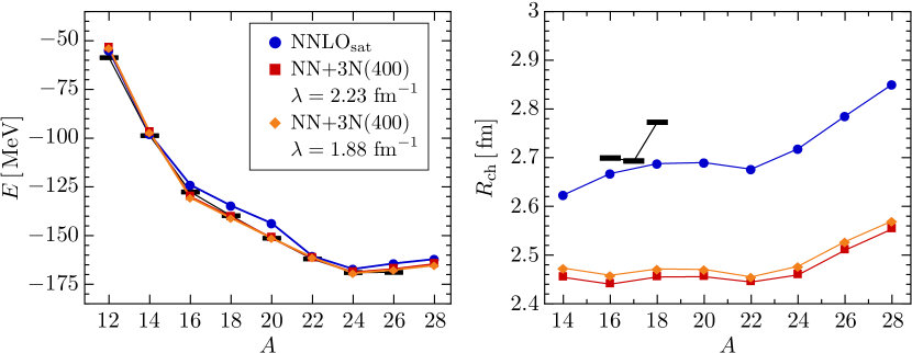
Figure 9.14: MR-IMSRG(2) ground-state energies and charge radii of the oxygen isotopes for $\text{NNLO}_{\text{sat}}$ and $NN\!+\!3N(400)$ at $\lambda=1.88,\ldots,2.24\,\text{fm}^{-1}$ ($e_{\text{max}}=14,E_{3\text{max}}=14$, and optimal $\hbar\omega$). Black bars indicate experimental data Wang:2012uq ; Angeli:2013rz .

The $NN+3N(400)$ Hamiltonian consists of the N³LO interaction by Entem and Machleidt Entem:2003th ; Machleidt:2011bh , with cutoff $\Lambda_{NN}=500\,\,\text{MeV}$, and a local NNLO interaction with a reduced cutoff $\Lambda_{NN}=400\,\,\text{MeV}$ Roth:2011kx ; Gazit:2009qf . The low-energy constants (LECs), i.e., the parameters of the chiral Hamiltonian, are entirely fixed by fitting data in the $A=2,3,4$ systems, and it is evolved to lower resolution scales $\lambda$ via free-space SRG, as discussed in Sec. 9.2.4. In contrast, the LECs of $\text{NNLO}_{\text{sat}}$ are also optimized with respect to selected many-body data Ekstrom:2015fk , and it is sufficiently soft that we use it as is.

While $NN+3N(400)$ gives a good reproduction of the oxygen ground-state energies, an issue with the Hamiltonian’s saturation properties is revealed by inspecting the oxygen charge radii (see Fig. 9.14). The theoretical charge radii are about 10% smaller than the experimental charge radius of ${}^{16}\mathrm{O}$, $R_{\text{ch}}=2.70\,\,\text{fm}$ Angeli:2013rz , and the sharp increase for ${}^{18}\mathrm{O}$ is missing entirely. The variation of $\lambda$ produces only a 0.2% change in the ground-state energies, but this is the result of a fine-tuned cancellation between induced $4N$ forces that are generated by the $NN$ and $3N$ pieces of the Hamiltonian, and should not be seen as representative for chiral interactions in general. The charge radii grow larger as $\lambda$ decreases, which is consistent with a study for light nuclei by Schuster et al.Schuster:2014oq . The authors found that two- and three-body terms that are induced by consistently evolving the charge radius operator to lower $\lambda$ have the opposite effect and reduce its expectation value. These terms have not been included here, but need to be considered for complete consistency in the future.

The MR-IMSRG(2) ground-state energies obtained with $\text{NNLO}_{\text{sat}}$ are slightly lower than those for $NN\!+\!3N(400)$ in the proton-rich isotopes ${}^{12,14}\mathrm{O}$, and above the $NN\!+\!3N(400)$ energies in ${}^{16-28}\mathrm{O}$. From ${}^{16-22}\mathrm{O}$, the $\text{NNLO}_{\text{sat}}$ ground-state energies exhibit a parabolic behavior as opposed to the essentially linear trend we find for $NN\!+\!3N(400)$. A possible cause is the inclusion of the ${}^{22,24}\mathrm{O}$ ground-state energies in the optimization protocol, which constrains the deviation of the energies from experimental data in these nuclei. $\text{NNLO}_{\text{sat}}$ predicts the drip line at ${}^{24}\mathrm{O}$, and the trend for the ${}^{26,28}\mathrm{O}$ resonance energies is similar to the $NN\!+\!3N(400)$ case. For $\text{NNLO}_{\text{sat}}$, the charge radii for the bound oxygen isotopes are about 10% larger than for $NN\!+\!3N(400)$, which is expected given the use of the ${}^{16}\mathrm{O}$ charge radius in the optimization of the LECs (also see Ref. Lapoux:2016xu ). For the resonant states, the increase is even larger, but continuum effects must be considered to make a meaningful comparison. We note that $\text{NNLO}_{\text{sat}}$ also fails to describe the sharp jump in $R_{\text{ch}}$ at ${}^{18}\mathrm{O}$.

9.4.3 Effective Hamiltonians

A recurring theme of this chapter has been the transformation of nuclear Hamiltonians to a shape that facilitates their subsequent application in many-body calculations. We have stressed this point in our discussion of the free-space SRG, in particular (see Sec. 9.2.4), but it applies to the IMSRG (or the MR-IMSRG) as well. Recall our application of the IMSRG to the pairing Hamiltonian in Sec. 9.3.6, where we primarily focused on how correlations that are usually probed by perturbative corrections are shuffled into the flowing ground-state energy $E(s)$ in the limit $s\to\infty$ (see Fig. 9.15). We can also interpret the results shown in this figure in a slightly different way: At any given value of $s$, $E(s)$ would result from a simple HF calculation with the Hamiltonian $\hat{H}(s)$, which has absorbed correlations because of an RG improvement. The result of the simple HF calculation approaches the exact result as we evolve, aside from truncation errors, of course. The same is true for the MBPT(2) and MBPT(3) calculations, summing $E(s)$ plus perturbative corrections through the indicated order. Of course, these approaches are already closer to the exact result in the first place.

Figure 9.15: IMSRG(2) flow for the ground state of the pairing Hamiltonian with $\delta=1.0,g=0.5$ (cf. Sec. 9.2.3). Calculations were performed with the White generator, Eq. (9.141). The figures shows the flowing ground-state energy $E(s)$ plus perturbative second and third-order energy corrections for $\hat{H}(s)$. The exact ground-state energy is indicated by the dashed line.

This example illustrates the potential benefits of using Hamiltonians that have been improved through IMSRG evolution as input for other many-body methods. In this section, we will briefly discuss applications in the traditional nuclear Shell model, which will give us access to a wealth of spectroscopic observables like excitation energies and transition rates. We will also look at the use of IMSRG Hamiltonians in Equation-of-Motion methods, which are an alternative approach to the computation of excited-state properties.

Non-Empirical Interactions for the Nuclear Shell Model

In IMSRG ground-state applications, we use the RG flows to decouple a suitable reference state from $npnh$ excitations (see Sec. 9.3.3). From a more general perspective, we can view this as a decoupling of different sectors of the many-body Hilbert space by driving the couplings of these sectors to zero. We are not forced to restrict the decoupling to a single state, but could target multiple states at once Tsukiyama:2012fk ; Parzuchowski:2016pi ; Hergert:2017kx — all we need to do is tailor our definition of the off-diagonal Hamiltonian to the problem, as in all SRG and IMSRG applications!

Figure 9.16: Separation of the single-particle basis into hole (h), valence particle (v) and non-valence particle (q) states. The Fermi energy of the fully occupied core, $\varepsilon_{F}$, is indicated by the red dashed line.

In the nuclear Shell model, we split the single-particle basis in our calculation into core or hole ($h$), valence particle ($v$) and non-valence particle ($q$) orbitals (see Fig. 9.16). The actual many-body calculation for a nucleus with $A$ nucleons is an exact diagonalization of the Hamiltonian matrix in a subspace of the Hilbert space that is spanned by configurations of the form

$$\,|{a^{\dagger}_{v_{1}}\ldots a^{\dagger}_{v_{A_{v}}}}\rangle\equiv a^{\dagger}_{v_{1}}\ldots a^{\dagger}_{v_{A_{v}}}\,|{\Phi}\rangle\,,$$ (9.219)

where $\,|{\Phi}\rangle$ is the wave function for a suitable core with $A_{c}$ nucleons, and the $A_{v}$ valence nucleons are distributed over the valence orbitals $v_{i}$ in all possible ways. Since the core is assumed to be inert, it can be viewed as a vacuum state for the valence configurations. The matrix representation of the Hamiltonian in the space spanned by these configurations is

$$\langle{v^{\prime}_{1}\ldots v^{\prime}_{A_{v}}}|\,{\hat{H}}\,|{v_{1}\ldots v_{A_{v}}}\rangle=\langle{\Phi}|\,{a_{v^{\prime}_{A_{v}}}\ldots a_{v^{\prime}_{1}}\hat{H}a^{\dagger}_{v_{1}}\ldots a^{\dagger}_{v_{A_{v}}}}\,|{\Phi}\rangle\,.$$ (9.220)

This expression suggests that we normal order the Hamiltonian and other operators with respect to the core wave function $\,|{\Phi}\rangle$, which can be obtained from a simple spherical HF calculation. The state $\,|{\Phi}\rangle$ takes on the role of the reference state for the IMSRG flow, but recent studies have shown that choosing either individual configurations for the target nucleus or ensembles of configurations as references will reduce truncation errors due to omitted induced terms, see Stroberg:2016fk ; Stroberg:2016th . When the resulting valence-space interactions are used to calculate nuclear ground-state energies, we find excellent agreement with direct IMSRG ground-state calculations, which indicates that the introduction of the inert core is justified, at least for the used $NN+3N$ forces with low resolution scales $\lambda$.

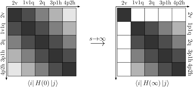
Figure 9.17: Schematic view of IMSRG valence-space decoupling for two valence nucleons (p$\,=\,$v, q).

We want to use the IMSRG evolution to decouple the configurations (9.219) from states that involve excitations of the core, just as in the ground-state calculations. In addition, we need to decouple them from states containing nucleons in non-valence particle states (see Fig. 9.17). Working in IMSRG(2) truncation, i.e., assuming up to two-body terms in $\hat{H}(s)$, we can identify the matrix elements that couple pairs of valence-space particles to $1q1v$, $2q$, $3p1h$, and $4p2h$ excitations, respectively, where $p=v,q$. For each type of matrix element, we show the antisymmetrized Goldstone diagrams Shavitt:2009 that represent the excitation process. Additional diagrams due to permutations of the nucleons or Hermitian adjoints are suppressed for brevity.

Diagrams (I) and (II) are eliminated if matrix elements of $f$ and $\Gamma$ that contain at least one q index are chosen to be off-diagonal. Diagrams (III) and (V) are eliminated by decoupling the reference-state, i.e., the core, which requires $f^{p}_{h}$ and $\Gamma^{pp^{\prime}}_{hh^{\prime}}$ to be off-diagonal (cf. Sec. 9.3.3). This only leaves diagram (IV), which vanishes if matrix elements of the type $\Gamma^{pp^{\prime}}_{vh}$ vanish. Thus, we define Tsukiyama:2012fk ; Hergert:2017kx

$$H_{od}\equiv\sum_{i\neq i^{\prime}}f^{i}_{i^{\prime}}\big{\{}\hat{A}^{i}_{i^{\prime}}\big{\}}+\frac{1}{4}\left(\sum_{pp^{\prime}hh^{\prime}}\Gamma^{pp^{\prime}}_{hh^{\prime}}\big{\{}\hat{A}^{pp^{\prime}}_{hh^{\prime}}\big{\}}+\sum_{pp^{\prime}vh}\Gamma^{pp^{\prime}}_{vh}\big{\{}\hat{A}^{pp^{\prime}}_{vh}\big{\}}+\sum_{pqvv^{\prime}}\Gamma^{pq}_{vv^{\prime}}\big{\{}\hat{A}^{pq}_{vv^{\prime}}\big{\}}\right)+\text{H.c.}\,.$$ (9.221)

This definition of the off-diagonal Hamiltonian holds for an arbitrary number of valence particles $A_{v}$. For $A_{v}=1$, diagram (II) vanishes, while diagrams (I) and (III)-(V) have the same topology, but one less spectator nucleons. Analogously, diagrams (I)-(V) merely contain additional spectator nucleons for $A_{v}>2$.

no.	type	diagram	energy difference $\Delta$
I	$\langle{2p}|\,{\hat{H}}\,|{2p}\rangle$		$f^{p}_{p}-f^{p^{\prime}}_{p^{\prime}}$
II	$\langle{2p}|\,{\hat{H}}\,|{2p}\rangle$		$f^{p}_{p}+f^{p^{\prime}}_{p^{\prime}}-f^{p^{\prime\prime}}_{p^{\prime\prime}}-f^{p^{\prime\prime\prime}}_{p^{\prime\prime\prime}}+\Gamma^{pp^{\prime}}_{pp^{\prime}}-\Gamma^{p^{\prime\prime}p^{\prime\prime\prime}}_{p^{\prime\prime}p^{\prime\prime\prime}}$
III	$\langle{3p1h}|\,{\hat{H}}\,|{2p}\rangle$		$f^{p}_{p}-f^{h}_{h}-\Gamma^{ph}_{ph}$
IV	$\langle{3p1h}|\,{\hat{H}}\,|{2p}\rangle$		$f^{p}_{p}+f^{p^{\prime}}_{p^{\prime}}-f^{p^{\prime\prime}}_{p^{\prime\prime}}-f^{h}_{h}+\Gamma^{pp^{\prime}}_{pp^{\prime}}-\Gamma^{ph}_{ph}-\Gamma^{p^{\prime}h}_{p^{\prime}h}$
V	$\langle{4p2h}|\,{\hat{H}}\,|{2p}\rangle$		$f^{p}_{p}+f^{p^{\prime}}_{p^{\prime}}-f^{h}_{h}-f^{h^{\prime}}_{h^{\prime}}+\Gamma^{pp^{\prime}}_{pp^{\prime}}+\Gamma^{hh^{\prime}}_{hh^{\prime}}-\Gamma^{ph}_{ph}-\Gamma^{p^{\prime}h^{\prime}}_{p^{\prime}h^{\prime}}-\Gamma^{ph^{\prime}}_{ph^{\prime}}-\Gamma^{p^{\prime}h}_{p^{\prime}h}$

Table 9.2: Classification of matrix elements of the many-body Hamiltonian in the many-body Hilbert space spanned by $(n+2)$p$n$h excitations of the reference state (cf. Fig. 9.17). For each matrix element, we show the corresponding antisymmetrized Goldstone diagrams Shavitt:2009 involving the one- and two-body parts of $\hat{H}$ (permutations involving spectator particles which are required by antisymmetry are implied), as well as the energy differences appearing in the matrix elements for $\eta(s)$ in each case (see text).

Using $\hat{H}_{od}$ in the construction of generators, we evolve the Hamiltonian by solving the IMSRG(2) flow equations (9.104)–(9.106). The evolved Hamiltonian is given by

$$\hat{H}(\infty)=E+\sum_{v}f^{v}_{v}\big{\{}\hat{A}^{v}_{v}\big{\}}+\frac{1}{4}\sum_{v_{i},v_{j},v_{k},v_{l}}\Gamma^{v_{i}v_{j}}_{v_{k}v_{l}}\big{\{}\hat{A}^{v_{i}v_{j}}_{v_{k}v_{l}}\big{\}}+\ldots\,,$$ (9.222)

where the explicitly shown terms are the core energy, single-particle energies, and two-body matrix elements that are used as input for a subsequent Shell model diagonalization.

A possible subtlety is associated with the treatment of the mass-number dependence of the intrinsic Hamiltonian (9.86). We interpret it as a dependence on the mass-number operator $\hat{A}$, which acts on the many-body states on which we are operating, i.e., configurations in the target nucleus, and therefore the mass number of the target should be used in the intrinsic Hamiltonian at all stages of a calculation Hergert:2009wh ; Stroberg:2016fk ; Stroberg:2016th . This is appropriate because the combined IMSRG + Shell model calculation is supposed to approximate the results of an exact diagonalization for that particular nucleus.

The naive computational scaling for the valence-decoupling procedure described here is $\mathscr{O}(N^{6})$, just like that of IMSRG(2) ground-state calculations. On 2015/16 computing hardware, typical evolutions require about 100-1000 core hours, assuming a single major shell as the valence space. The Shell model calculation is typically less expensive in that case. However, it will start to dominate the computational scaling as soon as we have to consider extended valence spaces consisting of two or more major shells, because of the factorial growth of the Shell model basis (cf. Sec. 9.2.3).

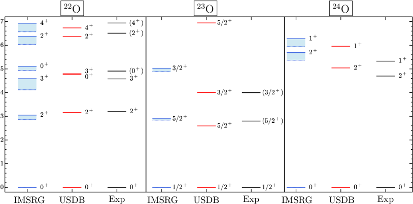
Figure 9.18: Excited-state spectra of ^22,23,24O based on the chiral $NN+3N(400)$ interaction with $\lambda=1.88\,\,\text{fm}^{-1}$, compared to results with the phenomenological USDB interaction Brown:2006fk and experimental data, see Bogner:2014tg ; Hergert:2017kx for full details. Dotted and solid lines are results for $\hbar\omega=20\,\,\text{MeV}$ and $\hbar\omega=24\,\,\text{MeV}$, respectively, which are shown as an indicator of convergence.

As an example, Fig. 9.18 shows the low-lying excitation spectra of ${}^{22-24}\mathrm{O}$ from Shell model calculations with IMSRG-derived valence-space interactions. These interactions were generated from an underlying chiral $NN+3N$ Hamiltonian consisting of the N³LO $NN$ interaction by Entem and Machleidt with $\Lambda_{NN}=500\,\,\text{MeV}$, and an NNLO $3N$ interaction with $\Lambda_{3N}=400\,\,\text{MeV}$, which has been evolved to $\lambda=1.88\,\,\text{fm}^{-1}$ Entem:2003th ; Machleidt:2011bh ; Gazit:2009qf ; Roth:2011kx (also cf. Secs. 9.2.4,9.4.2). We compare our results to the gold-standard phenomenological USDB interaction by Brown and Richter, which describes more than 600 ground-state and excitation energies in $sd-$shell ($8\leq Z,N\leq 20$) nuclei with an rms deviation of merely $\sim 130\,\,\text{keV}$ Brown:2006fk , and to experimental data. In the nuclei shown, the agreement is quite satisfactory given that the chiral input Hamiltonian is entirely fixed by $A\leq 4$ data. The IMSRG interactions turn out to perform quite well in the entire lower $sd-$shell, achieving an rms deviation of $\sim 580\,\,\text{keV}$ in about 150 states Stroberg:2016fk ; Hergert:2017kx . The chiral $3N$ interactions are found to be of crucial importance for the correct reproduction of level orderings and spacings.

Equation-of-Motion Methods

Equation-of-Motion (EOM) methods Rowe:1968eq are a useful alternative to the Shell model when it comes to the calculation of excited states, in particular when extended valence spaces lead to prohibitively large Shell model basis dimensions. In these approaches, the Schrödinger equation is rewritten in terms of ladder operators that create excited eigenstates from the exact ground state:

$$\hat{H}\,|{\Psi_{n}}\rangle=E_{n}\,|{\Psi}\rangle\qquad\longrightarrow\qquad\hat{H}\hat{X}^{\dagger}_{n}\,|{\Psi_{0}}\rangle=E_{n}\hat{X}^{\dagger}_{n}\,|{\Psi_{0}}\rangle\,.$$ (9.223)

Formally, $\hat{Q}^{\dagger}_{n}$ is given by the dyadic product $\,|{\Psi_{n}}\rangle\bra{\Psi_{0}}$, and by thinking of the exact eigenstates in a CI sense, it is easy to see that they can be expresed as a linear combination of up to $A$-body excitation and de-excitation operators acting on the ground state. We can further rewrite Eq. (9.223) as the Equation of Motion

$$[{\hat{H}},{\hat{X}^{\dagger}_{n}}]\,|{\Psi_{0}}\rangle=(E_{n}-E_{0})\hat{X}^{\dagger}_{n}\,|{\Psi_{0}}\rangle\equiv\omega_{n}\hat{X}^{\dagger}_{n}\,|{\Psi_{0}}\rangle\,,$$ (9.224)

and introduce systematic approximations to the $\hat{X}^{\dagger}_{n}$ and the ground-state $\,|{\Psi_{0}}\rangle$. For example, by replacing $\,|{\Psi_{0}}\rangle$ with a simple Slater determinant and using the ansatz

$$\hat{X}^{\dagger}_{n}=\sum_{k}X_{nk}a^{\dagger}_{k}\,,$$ (9.225)

we obtain Hartree-Fock theory, for

$$\hat{X}^{\dagger}_{n}=\sum_{ph}X^{(n)}_{ph}a^{\dagger}_{p}a_{h}\,,$$ (9.226)

we have the Tamm-Dancoff Approximation (TDA) for excited states, and

$$\hat{X}^{\dagger}_{n}=\sum_{ph}X^{(n)}_{ph}a^{\dagger}_{p}a_{h}-Y^{(n)}_{ph}a^{\dagger}_{h}a_{p}\,,$$ (9.227)

yields the Random Phase Approximation (RPA) in quasi-boson approximation Ring:1980bb ; Suhonen:2007wo . Plugging the Slater determinant reference state and the ansatz for the ladder operators into the Eq.  (9.224), we end up with a regular or a generalized eigenvalue problem, which we solve for the amplitudes appearing in the $\hat{X}^{\dagger}_{n}$ operators. Since the computed amplitudes can be used to improve the ground-state ansatz, it is usually possible to construct self-consistent solutions of the EoM (9.224) in a given truncation.

Since we have casually referred to the approximate ground state as a reference state already, it will not come as a surprise to our readers that we can quite naturally combine EOM methods with the IMSRG. Per construction, the reference state $\,|{\Phi_{0}}\rangle$ will be the ground state of the final IMSRG Hamiltonian

$$\mkern 3.0mu\overline{\mkern-3.0muH}\equiv\hat{U}(\infty)\hat{H}(0)\hat{U}^{\dagger}(\infty)$$ (9.228)

. Multiplying Eq. (9.224) by $\hat{U}(\infty)$ and recalling that

$$\hat{U}(\infty)\,|{\Psi_{0}}\rangle=\,|{\Phi_{0}}\rangle\,,$$ (9.229)

we obtain the unitarily transformed EOM

$$[{\mkern 3.0mu\overline{\mkern-3.0muH}},{\overline{X}^{\dagger}_{n}}]\,|{\Phi_{0}}\rangle=\omega_{n}\overline{X}^{\dagger}_{n}\,|{\Phi_{0}}\rangle\,.$$ (9.230)

The solutions $\overline{X}^{\dagger}_{n}$ can be used to obtain the eigenstates of the unevolved Hamiltonian via

$$\,|{\Psi_{n}}\rangle=\hat{U}^{\dagger}(\infty)\overline{X}^{\dagger}_{n}\,|{\Phi_{0}}\rangle\,.$$ (9.231)

In current applications, we include up to $2p2h$ excitations in the ladder operator Parzuchowski:2016pi :

$$\overline{X}^{\dagger}_{n}=\sum_{ph}\bar{X}^{(n)}_{ph}\big{\{}a^{\dagger}_{p}a_{h}\big{\}}+\frac{1}{4}\sum_{pp^{\prime}hh^{\prime}}\bar{X}^{(n)}_{pp^{\prime}hh^{\prime}}\big{\{}a^{\dagger}_{p}a^{\dagger}_{p^{\prime}}a_{h^{\prime}}a_{h}\big{\}}\,.$$ (9.232)

Note that the operator only contains excitation operators because de-excitation operators annihilate the reference state $\,|{\Phi_{0}}\rangle$ and therefore do not contribute in the EOM:

$$[{\big{\{}a^{\dagger}_{h}a^{\dagger}_{h^{\prime}}a_{p^{\prime}}a_{p}\big{\}}},{\overline{H}}]\,|{\Phi_{0}}\rangle=(\overline{H}-E)\big{\{}a^{\dagger}_{h}a^{\dagger}_{h^{\prime}}a_{p^{\prime}}a_{p}\big{\}}\,|{\Phi_{0}}\rangle=0\,.$$ (9.233)

The ladder operator $\overline{X}^{\dagger}$ can be systematically improved by including higher particle-hole excitations, until we reach the $ApAh$ level which would amount to an exact diagonalization of $\mkern 3.0mu\overline{\mkern-3.0muH}$. Denoting the operator rank of the ladder operator by $m$ and the IMSRG truncation by $n$, we refer to a specific combined scheme as EOM-IMSRG($m$,$n$).

Like TDA and RPA, the EOM (9.230) can be implemented as an eigenvalue problem that can be tackled with the Lanczos-Arnoldi or Davidson algorithms Lanczos:1950sp ; Arnoldi:1951kk ; Davidson:1989pi that are also used in CI approaches. As mentioned throughout this chapter, these algorithms only require knowledge of matrix-vector products. In the EOM-IMSRG, the required product is identified once we realize that the commutator in Eq. (9.230) can be rewritten as the connected product of $\mkern 3.0mu\overline{\mkern-3.0muH}$ and $\overline{X}^{\dagger}$:

$$[{\mkern 3.0mu\overline{\mkern-3.0muH}},{\overline{X}^{\dagger}_{n}}]=\{\mkern 3.0mu\overline{\mkern-3.0muH}\overline{X}^{\dagger}_{n}\}_{C}\,.$$ (9.234)

Thus, the matrix-vector product can be computed with the same commutator routines that are used in the evaluation of the IMSRG flow equations. Thus, the scaling of EOM-IMSRG($m$,$n$) is the same as that of the IMSRG($\max{m,n}$), e.g., $\mathscr{O}(N^{6})$ for the EOM-IMSRG(2,2) scheme that is the method we primarily use at this point Parzuchowski:2016pi .

Figure 9.19: EOM-IMSRG(2,2) excitation spectra of ${}^{14}\mathrm{C}$ and ${}^{22}\mathrm{O}$, calculated with the chiral $NN+3N(400)$ Hamiltonian for $\lambda=1.88\,\,\text{fm}^{-1}$ ( cf. Fig. 9.18), compared with experimental data.

In Fig. 9.19, we show sample spectra of ${}^{14}\mathrm{C}$ and ${}^{22}\mathrm{O}$ from EOM-IMSRG(2,2) calculations with the chiral $NN+3N(400)$ Hamiltonian ($\lambda=1.88\,\,\text{fm}^{-1}$). We see that certain levels seem to be reproduced quite well, while experimentally observed states below $8\,\,\text{MeV}$ are either missing in the calculation in the case of ${}^{14}\mathrm{C}$), or found at higher excitation theoretical excitation energy in the case of ${}^{22}\mathrm{O}$. In the latter case, we can compare the EOM-IMSRG(2,2) calculation to the IMSRG+SM spectrum shown in Fig. 9.18, in which the group of $2^{+},3^{+},4^{+}$ states is found much closer to their experimental counterparts. This suggests that the overestimation of the excitation energy in the EOM approach is caused by the truncation of the ladder operator at the $2p2h$ level, while the Shell model contains all allowed $npnh$ excitations in the valence space. Conversely, we can conclude that the states that the EOM-IMSRG(2,2) is reproducing well are dominated by $1p1h$ and $2p2h$ excitations Parzuchowski:2016pi .

An advantage of the EOM-IMSRG(2,2) over the IMSRG+SM is that it allows us to compute negative parity states, to the level of accuracy that the truncation allows. In the Shell model, the description of such states requires a valence space consisting of two major shells, which usually makes the exact diagonalization prohibitively expensive, especially in $sd-$shell nuclei and beyond.

9.4.4 Final Remarks

Superficially, the discussion in Sec. 9.4 focused on three different subject areas, namely Magnus methods, MR-IMSRG, and the construction of effective Hamiltonians, but we expect that our readers can already tell that these directions are heavily intertwined.

The Magnus formulation of the IMSRG will greatly facilitate the evaluation of general observables not just in the regular single-reference version of the method, but also in the MR-IMSRG. Magnus methods can also be readily adapted to the construction of effective valence-space operators besides the nuclear interaction, e.g., radii and electroweak transitions. In addition, it allows us to construct systematic and computationally tractable approximations to the full IMSRG(3) Morris:2016xp ; Parzuchowski:2016pi , similar to the non-iterative treatment of triples in Coupled Cluster methods Taube:2008kx ; Taube:2008vn ; Piecuch:2005dp ; Binder:2013fk .

While the current version of our EOM technology is based on the single-reference IMSRG, we will formulate a multireference EOM scheme based on final Hamiltonians from the MR-IMSRG evolution next. Such a MR-EOM-IMSRG will hold great potential for the description of excitations in deformed or weakly bound nuclei, which would require excessively large valence spaces in traditional CI approaches, and at the same time require an explicit treatment of static correlations that the uncorrelated reference wave functions used in the IMSRG and EOM-IMSRG cannot provide.

The MR-IMSRG has also recently been used to pre-diagonalize Hamiltonians that serve as input for the No-Core Shell Model (NCSM), merging the two approaches into an iterative scheme that we call the In-Medium NCSM (IM-NCSM for short) Gebrerufael:2016rp . In this combined approach, we can converge NCSM results in model spaces whose dimensions are orders of magnitude smaller than those of the regular NCSM or its importance-truncated variant Roth:2007fk ; Roth:2009eu ; Roth:2014fk , which should significantly expand its range of applicability. A similar idea might be used fruitfully in the traditional Shell model with a core as well, where the use of statically correlated reference states and an MR-IMSRG evolution might help to overcome shortcomings in the Shell model interactions for specific nuclei.

9.5 Conclusions

In this chapter, we have presented a pedagogical introduction to the SRG and IMSRG, and discussed their applications in the context of the nuclear many-body problem. The former has become maybe the most popular tool for pre-processing nuclear interactions and operators, leading to vast improvements in the rate of convergence of many-body calculations, and extending the range of nuclei that can be tackled in ab initio approaches Barrett:2013oq ; Hagen:2014ve ; Binder:2014fk ; Soma:2014eu ; Hergert:2016jk ; Hergert:2017kx . The IMSRG implements SRG concepts directly in the $A$-body system, relying on normal-ordering methods to control the size of induced operators and make systematic truncations feasible. As we have demonstrated through a variety of applications, the IMSRG is an extremely versatile and powerful addition to the canon of quantum many-body methods. In Sec. 9.4, we have given an overview of the main thrusts of current IMSRG research, and we hope that our readers will be inspired to contribute to these developments, or find ways in which the IMSRG framework can be useful to their own research programs.

The explicit RG aspect of the IMSRG framework is a unique feature that sets it apart from most other many-body methods on the market. When the comparison with those other methods and experimental data is our first and foremost concern, we are primarily interested in the $s\to\infty$ limit of the IMSRG or MR-IMSRG evolution, but the flow trajectory is an enormous source of additional insight. By studying the flows, not just the final fixed points, we can gain a new understanding of how many-body correlations are reshuffled between the wave function and the Hamiltonian, or different pieces of the Hamiltonian, making transparent what is only implicitly assumed in other methods. Like in the free-space SRG (or other RG methods), we have the freedom to work at intermediate values of $s$ if this is more practical than working at $s=0$ or in the limit $s\to\infty$, especially if either of these extremes would lead to the accrual of unacceptable numerical errors in our results (see, e.g., Gebrerufael:2016rp ; Li:2015nq ; Li:2016rm ). This is the inherent power of a framework that integrates many-body and renormalization group techniques, and the reason why we consider the IMSRG to be an extremely valuable tool for quantum many-body theory.

9.6 Exercises and Projects

Prove that the two forms of the intrinsic kinetic energy operator given in Eqs. (9.54) and (9.55) are equivalent.

Now consider the expectation values of the two forms of $\hat{T}_{\text{int}}$ in a state that does not have a fixed particle number, e.g., as in Bardeen-Cooper-Schrieffer (BCS) Bardeen:1957bz ; Bardeen:1957tv or Hartree-Fock-Bogoliubov (HFB) theory (see, e.g., Ring:1980bb ). Expand the $\frac{1}{\hat{A}}$ dependence of Eqs. (9.54) and (9.55) into series around $\langle{\hat{A}}\rangle$ by introducing $\Delta\hat{A}=\hat{A}-\langle{\hat{A}}\rangle$, and compare the series expansions order by order. (A thorough discussion of the issue can be found in Hergert:2009wh .)

Prove that the expectation value of a normal-ordered operator in the reference state vanishes (Eq. (9.84)):

$$\langle{\Phi}|\,{\big{\{}a^{\dagger}_{i_{1}}\ldots a_{j_{1}}\big{\}}}\,|{\Phi}\rangle=0\,.$$ (9.235)

Start by considering a one-body operator, and extend your result to the general case by induction.

Show that $a^{\dagger}_{i}$ and $a_{j}$ anticommute freely in a normal-ordered string (Eq. (9.85)).

$$\big{\{}\ldots a^{\dagger}_{i}a_{j}\ldots\big{\}}=-\big{\{}\ldots a_{j}a^{\dagger}_{i}\ldots\big{\}}\,.$$ (9.236)

Consider the one-body case first, as in problem 9.6(a).

Prove the following schematic expression for products of normal-ordered operators:

$$\hat{A}^{[M]}\hat{B}^{[N]}=\sum_{k=|M-N|}^{M+N}\hat{C}^{[k]}\,.$$ (9.237)

Show that the following rule applies for commutators of normal-ordered operators:

$$[{\hat{A}^{[M]}},{\hat{B}^{[N]}}]=\sum_{k=|M-N|}^{M+N-1}\hat{C}^{[k]}\,.$$ (9.238)

Thus, the largest particle rank appearing in the expansion of the commutator of normal-ordered $M-$ and $N-$body operators is $M+N-1$.

We can view the free-space operators as being normal-ordered with respect to the vacuum state. How are the expansion formulas for products and commutators modified in that case?

Use Wick’s theorem to show that the basis consisting of a Slater determinant $\,|{\Phi}\rangle$ and its particle-hole excitations,

$$\,|{\Phi}\rangle,\,\big{\{}a^{\dagger}_{p}a_{h}\big{\}}\,|{\Phi}\rangle,\,\big{\{}a^{\dagger}_{p}a^{\dagger}_{p^{\prime}}a_{h^{\prime}}a_{h}\big{\}}\,|{\Phi}\rangle,\ldots\,,$$ (9.239)

is orthogonal if the underlying single-particle basis is orthonormal.

Validate the leading-order perturbative expression for the Wegner generator, Eq. (9.153).

Let us now assume that we have used a Slater determinant reference state that has not been optimized by performing a Hartree-Fock calculation. Using Epstein-Nesbet partioning, the one-body part of the off-diagonal Hamiltonian is then counted as $f^{od}_{ij}=\mathscr{O}(g)$ instead of $\mathscr{O}(g^{2})$ during the flow. Show that the one-body part of the Wegner generator has the following perturbative expansion in this case:

$$\eta_{ij}=\left(f^{d}_{ii}-f^{d}_{jj}-(n_{i}-n_{j})\Gamma^{d}_{ijij}\right)f^{od}_{ij}+\mathscr{O}(g^{2})\,.$$ (9.240)

Interpret the expression in the parentheses.

Project: Optimization of the IMSRG(2) Code
In Sec. 9.3.5, we mention several ways of optimizing the performance of the Python code, like taking into account antisymmetry of two-body (and three-body) states, or exploiting symmetries and the resulting block structures.

Optimize the storage requirements and speed of the Python code by taking the antisymmetry of states as well as the Hermiticity (anti-Hermiticity) of $\hat{H}$ ($\eta$) into account.

Identify the symmetries of the pairing Hamiltonian, and construct a variant of imsrg_pairing.py that is explicitly block diagonal in the irreducible representations of the corresponding symmetry group.

A significant portion of the code imsrg_pairing.py consists of infrastructure routines that are used to convert between one- and two-body bases. We could avoid this inversion if we treat $\Gamma$ and the two-body part of the generator as rank-four tensors instead of matrices. NumPy offers tensor routines that can be used to evaluate tensor contractions and products, in particular numpy.tensordot(). Rewrite imsrg_pairing.py in terms of tensors, and compare the performance of your new code to the original version.

Project: IMSRG(3) for the Pairing Hamiltonian
Throughout this chapter, we used a single-particle basis consisting of only 8 states in our discussions of the pairing Hamiltonian. For such a small basis size, it is possible to implement to include explicit 3N operators in the IMSRG evoltion, that is, to work in the IMSRG(3) scheme.

Derive the IMSRG(3) flow equations. (Note: compare your results with Ref. Hergert:2016jk ).

Implement the IMSRG(3). The Python code discussed in Sec. 9.3.5 provides a good foundation, but you may find it necessary to switch to a language like C/C++ or Fortran for performance reasons.

“Interpolate” between IMSRG(2) and IMSRG(3) by selectively activating flow equation terms, and document the impact of these intermediate steps.

Appendix: Products and Commutators of Normal-Ordered Operators

In this appendix, we collect the basic expressions for products and commutators of normal-ordered one- and two-body operators. All single-particle indices refer to the natural orbital basis, where the one-body density matrix is diagonal

$$\rho_{kl}=\langle{\Phi}|\,{a^{\dagger}_{l}a_{k}}\,|{\Phi}\rangle=n_{k}\delta_{kl}\,,\quad n_{k}\in\{0,1\}\,,$$ (9.241)

(notice the convention for the indices of $\rho$, cf. Ring:1980bb ). We also define the hole density matrix

$$\bar{\rho}_{kl}\equiv\langle{\Phi}|\,{a_{k}a^{\dagger}_{l}}\,|{\Phi}\rangle=\delta_{kl}-\rho_{kl}\equiv\bar{n}_{k}\delta_{kl}$$ (9.242)

whose eigenvalues are

$$\bar{n}_{k}=1-n_{k}\,,$$ (9.243)

i.e., 0 for occupied and 1 for unoccupied single-particle states. Finally, we will again use the permutation symbol $\hat{P}_{ij}$ to interchange the indices in any expression,

$$\hat{P}_{ij}g(\ldots,i,\ldots,j)\equiv g(\ldots,j,\ldots,i)\,$$ (9.244)

(see Sec. 9.3 and chapter 8).

Operator Products

$$\big{\{}a^{\dagger}_{a}a_{b}\big{\}}\big{\{}a^{\dagger}_{k}a_{l}\big{\}} =\big{\{}a^{\dagger}_{a}a^{\dagger}_{k}a_{l}a_{b}\big{\}}-n_{a}\delta_{al}\big{\{}a^{\dagger}_{k}a_{b}\big{\}}+\bar{n}_{b}\delta_{bk}\big{\{}a^{\dagger}_{a}a_{l}\big{\}}+n_{a}\bar{n}_{b}\delta_{al}\delta_{bk}$$ (9.245)

$$\big{\{}a^{\dagger}_{a}a_{b}\big{\}}\big{\{}a^{\dagger}_{k}a^{\dagger}_{l}a_{n}a_{m}\big{\}} =\big{\{}a^{\dagger}_{a}a^{\dagger}_{k}a^{\dagger}_{l}a_{n}a_{m}a_{b}\big{\}}+\left(1-\hat{P}_{mn}\right)n_{a}\delta_{an}\big{\{}a^{\dagger}_{k}a^{\dagger}_{l}a_{m}a_{b}\big{\}}-\left(1-\hat{P}_{kl}\right)\bar{n}_{b}\delta_{bl}\big{\{}a^{\dagger}_{a}a^{\dagger}_{k}a_{n}a_{m}\big{\}}$$

$$\hphantom{=}-\left(1-\hat{P}_{kl}\right)\left(1-\hat{P}_{mn}\right)n_{a}\bar{n}_{b}\delta_{am}\delta_{bl}\big{\{}a^{\dagger}_{k}a_{n}\big{\}}$$ (9.246)

$$\big{\{}a^{\dagger}_{a}a^{\dagger}_{b}a_{d}a_{c}\big{\}}\big{\{}a^{\dagger}_{k}a^{\dagger}_{l}a_{n}a_{m}\big{\}}$$

$$=\big{\{}a^{\dagger}_{a}a^{\dagger}_{b}a^{\dagger}_{k}a^{\dagger}_{l}a_{n}a_{m}a_{d}a_{c}\big{\}}$$

$$\hphantom{=}+(1-\hat{P}_{ab})(1-\hat{P}_{mn})n_{a}\delta_{am}\big{\{}a^{\dagger}_{b}a^{\dagger}_{k}a^{\dagger}_{l}a_{n}a_{d}a_{c}\big{\}}-(1-\hat{P}_{cd})(1-\hat{P}_{kl})\bar{n}_{c}\delta_{ck}\big{\{}a^{\dagger}_{a}a^{\dagger}_{b}a^{\dagger}_{l}a_{n}a_{m}a_{d}\big{\}}$$

$$\hphantom{=}+(1-\hat{P}_{mn})n_{a}n_{b}\delta_{am}\delta_{bn}\big{\{}a^{\dagger}_{k}a^{\dagger}_{l}a_{d}a_{c}\big{\}}+(1-\hat{P}_{cd})\bar{n}_{c}\bar{n}_{d}\delta_{ck}\delta_{dl}\big{\{}a^{\dagger}_{a}a^{\dagger}_{b}a_{n}a_{m}\big{\}}$$

$$\hphantom{=}+(1-\hat{P}_{ab})(1-\hat{P}_{cd})(1-\hat{P}_{kl})(1-\hat{P}_{mn})n_{a}\bar{n}_{c}\delta_{am}\delta_{ck}\big{\{}a^{\dagger}_{b}a^{\dagger}_{l}a_{n}a_{d}\big{\}}$$

$$\hphantom{=}+(1-\hat{P}_{ab})(1-\hat{P}_{kl})(1-\hat{P}_{mn})n_{b}\bar{n}_{c}\bar{n}_{d}\delta_{bn}\delta_{ck}\delta_{dl}\big{\{}a^{\dagger}_{a}a_{m}\big{\}}$$

$$\hphantom{=}+(1-\hat{P}_{cd})(1-\hat{P}_{kl})(1-\hat{P}_{mn})\bar{n}_{d}n_{a}n_{b}\delta_{dl}\delta_{an}\delta_{bm}\big{\{}a^{\dagger}_{k}a_{c}\big{\}}$$

$$\hphantom{=}+(1-\hat{P}_{kl})(1-\hat{P}_{mn})n_{a}n_{b}\bar{n}_{c}\bar{n}_{d}\delta_{am}\delta_{bn}\delta_{ck}\delta_{dl}$$ (9.247)

Commutators

$$[{\big{\{}a^{\dagger}_{a}a_{b}\big{\}}},{\big{\{}a^{\dagger}_{k}a_{l}\big{\}}}] =\delta_{bk}\big{\{}a^{\dagger}_{a}a_{l}\big{\}}-\delta_{al}\big{\{}a^{\dagger}_{k}a_{b}\big{\}}+(n_{a}-n_{b})\delta_{al}\delta_{bk}$$ (9.248)

$$[{\big{\{}a^{\dagger}_{a}a_{b}\big{\}}},{\big{\{}a^{\dagger}_{k}a^{\dagger}_{l}a_{n}a_{m}\big{\}}}] =\left(1-\hat{P}_{kl}\right)\delta_{bk}\big{\{}a^{\dagger}_{a}a^{\dagger}_{l}a_{n}a_{m}\big{\}}-\left(1-\hat{P}_{mn}\right)\delta_{am}\big{\{}a^{\dagger}_{k}a^{\dagger}_{l}a_{n}a_{b}\big{\}}$$

$$\hphantom{=}+\left(1-\hat{P}_{kl}\right)\left(1-\hat{P}_{mn}\right)(n_{a}-n_{b})\delta_{an}\delta_{bl}\big{\{}a^{\dagger}_{k}a_{m}\big{\}}$$ (9.249)

$$[{\big{\{}a^{\dagger}_{a}a^{\dagger}_{b}a_{d}a_{c}\big{\}}},{\big{\{}a^{\dagger}_{k}a^{\dagger}_{l}a_{n}a_{m}\big{\}}}]$$

$$=\left(1-\hat{P}_{ab}\right)\left(1-\hat{P}_{mn}\right)\delta_{am}\big{\{}a^{\dagger}_{b}a^{\dagger}_{k}a^{\dagger}_{l}a_{n}a_{d}a_{c}\big{\}}-\left(1-\hat{P}_{cd}\right)\left(1-\hat{P}_{kl}\right)\delta_{kc}\big{\{}a^{\dagger}_{a}a^{\dagger}_{b}a^{\dagger}_{l}a_{n}a_{m}a_{d}\big{\}}$$

$$\hphantom{=}+(1-\hat{P}_{cd})\left(\bar{n}_{c}\bar{n}_{d}-n_{c}n_{d}\right)\delta_{ck}\delta_{dl}\big{\{}a^{\dagger}_{a}a^{\dagger}_{b}a_{n}a_{m}\big{\}}+(1-\hat{P}_{ab})\left(n_{a}n_{b}-\bar{n}_{a}\bar{n}_{b}\right)\delta_{am}\delta_{bn}\big{\{}a^{\dagger}_{k}a^{\dagger}_{l}a_{d}a_{c}\big{\}}$$

$$\hphantom{=}+(1-\hat{P}_{ab})(1-\hat{P}_{cd})(1-\hat{P}_{kl})(1-\hat{P}_{mn})\left(n_{b}-n_{d}\right)\delta_{bn}\delta_{dl}\big{\{}a^{\dagger}_{a}a^{\dagger}_{k}a_{m}a_{c}\big{\}}$$

$$\hphantom{=}+(1-\hat{P}_{ab})(1-\hat{P}_{mn})\left(n_{b}\bar{n}_{c}\bar{n}_{d}-\bar{n}_{b}n_{c}n_{d}\right)\delta_{bn}\delta_{ck}\delta_{dl}\big{\{}a^{\dagger}_{a}a_{m}\big{\}}$$

$$\hphantom{=}-(1-\hat{P}_{cd})(1-\hat{P}_{kl})\left(n_{d}\bar{n}_{a}\bar{n}_{b}-\bar{n}_{d}n_{a}n_{b}\right)\delta_{dl}\delta_{am}\delta_{bn}\big{\{}a^{\dagger}_{k}a_{c}\big{\}}$$

$$\hphantom{=}+(1-\hat{P}_{ab})(1-\hat{P}_{cd})\left(n_{a}n_{b}\bar{n}_{c}\bar{n}_{d}-\bar{n}_{a}\bar{n}_{b}n_{c}n_{d}\right)\delta_{am}\delta_{bn}\delta_{ck}\delta_{dl}$$ (9.250)

References

- (1) J.D. Jackson, Classical electrodynamics, 3rd edn. (Wiley, New York, NY, 1999)
- (2) E. Fermi, Zeitschrift für Physik 88, 161 (1934)
- (3) W. Detmold, Nuclear Physics from Lattice QCD (Springer International Publishing, Cham, 2015), p. 153
- (4) D.J. Gross, F. Wilczek, Phys. Rev. Lett. 30, 1343 (1973)
- (5) H.D. Politzer, Phys. Rev. Lett. 30, 1346 (1973)
- (6) E. Epelbaum, H.W. Hammer, U.G. Meißner, Rev. Mod. Phys. 81, 1773 (2009)
- (7) R. Machleidt, D. Entem, Phys. Rep. 503, 1 (2011)
- (8) E. Epelbaum, H. Krebs, U.G. Meißner, Phys. Rev. Lett. 115, 122301 (2015)
- (9) D.R. Entem, N. Kaiser, R. Machleidt, Y. Nosyk, Phys. Rev. C 91, 014002 (2015)
- (10) A. Gezerlis, I. Tews, E. Epelbaum, M. Freunek, S. Gandolfi, K. Hebeler, A. Nogga, A. Schwenk, Phys. Rev. C 90, 054323 (2014)
- (11) J.E. Lynn, I. Tews, J. Carlson, S. Gandolfi, A. Gezerlis, K.E. Schmidt, A. Schwenk, Phys. Rev. Lett. 116, 062501 (2016)
- (12) S. Pastore, L. Girlanda, R. Schiavilla, M. Viviani, R.B. Wiringa, Phys. Rev. C 80, 034004 (2009)
- (13) S. Pastore, L. Girlanda, R. Schiavilla, M. Viviani, Phys. Rev. C 84, 024001 (2011)
- (14) M. Piarulli, L. Girlanda, L.E. Marcucci, S. Pastore, R. Schiavilla, M. Viviani, Phys. Rev. C 87, 014006 (2013)
- (15) S. Kölling, E. Epelbaum, H. Krebs, U.G. Meißner, Phys. Rev. C 80, 045502 (2009)
- (16) S. Kölling, E. Epelbaum, H. Krebs, U.G. Meißner, Phys. Rev. C 84, 054008 (2011)
- (17) A. Ekström, G.R. Jansen, K.A. Wendt, G. Hagen, T. Papenbrock, B.D. Carlsson, C. Forssén, M. Hjorth-Jensen, P. Navrátil, W. Nazarewicz, Phys. Rev. C 91, 051301 (2015)
- (18) A.M. Shirokov, I.J. Shin, Y. Kim, M. Sosonkina, P. Maris, J.P. Vary, Physics Letters B 761, 87 (2016)
- (19) G.P. Lepage, (1989)
- (20) G.P. Lepage, (1997)
- (21) S.K. Bogner, T.T.S. Kuo, A. Schwenk, Phys. Rep. 386, 1 (2003)
- (22) S.K. Bogner, R.J. Furnstahl, R.J. Perry, Phys. Rev. C 75, 061001(R) (2007)
- (23) S.K. Bogner, R.J. Furnstahl, A. Schwenk, Prog. Part. Nucl. Phys. 65, 94 (2010)
- (24) R.J. Furnstahl, K. Hebeler, Rep. Prog. Phys. 76, 126301 (2013)
- (25) H.A. Bethe, Ann. Rev. Nucl. Sci. 21, 93 (1971)
- (26) W. Polyzou, W. Glöckle, Few-Body Systems 9, 97 (1990)
- (27) K.A. Brueckner, C.A. Levinson, H.M. Mahmoud, Phys. Rev. 95, 217 (1954)
- (28) K.A. Brueckner, C.A. Levinson, Phys. Rev. 97, 1344 (1955)
- (29) H.A. Bethe, J. Goldstone, Proceedings of the Royal Society of London A: Mathematical, Physical and Engineering Sciences 238, 551 (1957)
- (30) J. Goldstone, Proc. Roy. Soc. Lond. A Math. Phys. Eng. Sci. 239, 267 (1957)
- (31) B.D. Day, Rev. Mod. Phys. 39, 719 (1967)
- (32) B.H. Brandow, Rev. Mod. Phys. 39, 771 (1967)
- (33) B.R. Barrett, M.W. Kirson, Nucl. Phys. A 148, 145 (1970)
- (34) M.W. Kirson, Annals of Physics 66, 624 (1971)
- (35) B.R. Barrett, Physics Letters B 38, 371 (1972)
- (36) M.W. Kirson, Annals of Physics 82, 345 (1974)
- (37) P. Goode, M.W. Kirson, Physics Letters B 51, 221 (1974)
- (38) J.P. Vary, P.U. Sauer, C.W. Wong, Phys. Rev. C 7, 1776 (1973)
- (39) S.D. Glazek, K.G. Wilson, Phys. Rev. D 48, 5863 (1993)
- (40) F. Wegner, Ann. Phys. (Leipzig) 3, 77 (1994)
- (41) S.K. Bogner, R.J. Furnstahl, S. Ramanan, A. Schwenk, Nucl. Phys. A 773, 203 (2006)
- (42) R. Roth, J. Langhammer, Phys. Lett. B 683, 272 (2010)
- (43) A. Tichai, J. Langhammer, S. Binder, R. Roth, Physics Letters B 756, 283 (2016)
- (44) B.R. Barrett, P. Navrátil, J.P. Vary, Prog. Part. Nucl. Phys. 69, 131 (2013)
- (45) E.D. Jurgenson, P. Maris, R.J. Furnstahl, P. Navrátil, W.E. Ormand, J.P. Vary, Phys. Rev. C 87, 054312 (2013)
- (46) H. Hergert, S. Binder, A. Calci, J. Langhammer, R. Roth, Phys. Rev. Lett. 110, 242501 (2013)
- (47) R. Roth, A. Calci, J. Langhammer, S. Binder, Phys. Rev. C 90, 024325 (2014)
- (48) S. Binder, J. Langhammer, A. Calci, R. Roth, Phys. Lett. B 736, 119 (2014)
- (49) G. Hagen, T. Papenbrock, M. Hjorth-Jensen, D.J. Dean, Rep. Prog. Phys. 77, 096302 (2014)
- (50) G. Hagen, M. Hjorth-Jensen, G.R. Jansen, T. Papenbrock, Phys. Scripta 91, 063006 (2016)
- (51) K. Tsukiyama, S.K. Bogner, A. Schwenk, Phys. Rev. Lett. 106, 222502 (2011)
- (52) H. Hergert, S.K. Bogner, S. Binder, A. Calci, J. Langhammer, R. Roth, A. Schwenk, Phys. Rev. C 87, 034307 (2013)
- (53) H. Hergert, S.K. Bogner, T.D. Morris, A. Schwenk, K. Tsukiyama, Phys. Rep. 621, 165 (2016)
- (54) S. Kehrein, The Flow Equation Approach to Many-Particle Systems, Springer Tracts in Modern Physics, vol. 237 (Springer Berlin / Heidelberg, 2006)
- (55) C. Heidbrink, G. Uhrig, Eur. Phys. J. B 30, 443 (2002). 10.1140/epjb/e2002-00401-9
- (56) N.A. Drescher, T. Fischer, G.S. Uhrig, Eur. Phys. J. B 79, 225 (2011). 10.1140/epjb/e2010-10723-6
- (57) H. Krull, N.A. Drescher, G.S. Uhrig, Phys. Rev. B 86, 125113 (2012)
- (58) B. Fauseweh, G.S. Uhrig, Phys. Rev. B 87, 184406 (2013)
- (59) J. Krones, G.S. Uhrig, Phys. Rev. B 91, 125102 (2015)
- (60) I. Shavitt, R.J. Bartlett, Many-Body Methods in Chemistry and Physics: MBPT and Coupled-Cluster Theory (Cambridge University Press, 2009)
- (61) S.R. White, J. Chem. Phys. 117, 7472 (2002)
- (62) T. Yanai, G.K.L. Chan, J. Chem. Phys. 127, 104107 (2007)
- (63) H. Nakatsuji, Phys. Rev. A 14, 41 (1976)
- (64) D. Mukherjee, W. Kutzelnigg, J. Chem. Phys. 114, 2047 (2001)
- (65) D.A. Mazziotti, Phys. Rev. Lett. 97, 143002 (2006)
- (66) F.A. Evangelista, J. Chem. Phys. 141, 054109 (2014)
- (67) V. Bach, J.B. Bru, Journal of Evolution Equations 10, 425 (2010)
- (68) B. Boutin, N. Raymond, Journal of Evolution Equations p. 1 (2016)
- (69) R. Brockett, Linear Algebra and its Applications 146, 79 (1991)
- (70) M.T. Chu, Fields Institute Communications 3, 87 (1994)
- (71) M.T. Chu, Linear Algebra and its Applications 215, 261 (1995)
- (72) T.D. Morris, N.M. Parzuchowski, S.K. Bogner, Phys. Rev. C 92, 034331 (2015)
- (73) H. Hergert, Phys. Scripta 92, 023002 (2017)
- (74) G. Golub, C. Van Loan, Matrix Computations. Johns Hopkins Studies in the Mathematical Sciences (Johns Hopkins University Press, 2013)
- (75) W.H. Press, S.A. Teukolsky, W.T. Vetterling, B.P. Flannery, Numerical Recipes: The Art of Scientific Computing, 3rd edn. (Cambridge University Press, 2007)
- (76) L.F. Shampine, M.K. Gordon, Computer Solution of Ordinary Differential Equations: The Initial Value Problem (W. H. Freeman, San Francisco, 1975)
- (77) R.H. Landau, M.J. Paez, C.C. Bordeianu, A Survey of Computational Physics: Introductory Computational Science (Princeton University Press, 2012)
- (78) M. Hjorth-Jensen, Computational physics (2015)
- (79) A.C. Hindmarsh, ODEPACK, A Systematized Collection of ODE Solvers (North-Holland Publishing Company, Amsterdam, 1983), IMACS Transactions on Scientific Computation, vol. 1, p. 54
- (80) K. Radhakrishnan, A.C. Hindmarsh, Description and use of lsode, the livermore solver for ordinary differential equations. Tech. rep., Lawrence Livermore National Laboratory (1993)
- (81) P.N. Brown, A.C. Hindmarsh, Applied Mathematics and Computation 31, 40 (1989)
- (82) C. Lanczos, J. Res. Nat’l Bur. Std. 45, 255 (1950)
- (83) W.E. Arnoldi, Quarterly of Applied Mathematics 9, 17 (1951)
- (84) E.R. Davidson, Computer Physics Communications 53, 49 (1989)
- (85) C. Yang, H.M. Aktulga, P. Maris, E. Ng, J.P. Vary, in Proceedings of International Conference ‘Nuclear Theory in the Supercomputing Era — 2013’ (NTSE-2013), Ames, IA, USA, May 13–17, 2013., ed. by A.M. Shirokov, A.I. Mazur (2013), p. 272
- (86) H. Hergert, R. Roth, Phys. Lett. B 682, 27 (2009)
- (87) R.B. Wiringa, V.G.J. Stoks, R. Schiavilla, Phys. Rev. C 51, 38 (1995)
- (88) J. Carlson, S. Gandolfi, F. Pederiva, S.C. Pieper, R. Schiavilla, K.E. Schmidt, R.B. Wiringa, Rev. Mod. Phys. 87, 1067 (2015)
- (89) J.D. Holt, T.T.S. Kuo, G.E. Brown, S.K. Bogner, Nucl. Phys. A 733, 153 (2004)
- (90) K.A. Wendt, R.J. Furnstahl, R.J. Perry, Phys. Rev. C 83, 034005 (2011)
- (91) E.R. Anderson, S.K. Bogner, R.J. Furnstahl, R.J. Perry, Phys. Rev. C 82, 054001 (2010)
- (92) M.D. Schuster, S. Quaglioni, C.W. Johnson, E.D. Jurgenson, P. Navrátil, Phys. Rev. C 90, 011301 (2014)
- (93) S.N. More, S. König, R.J. Furnstahl, K. Hebeler, Phys. Rev. C 92, 064002 (2015)
- (94) E.D. Jurgenson, P. Navrátil, R.J. Furnstahl, Phys. Rev. Lett. 103, 082501 (2009)
- (95) K. Hebeler, Phys. Rev. C 85, 021002 (2012)
- (96) K.A. Wendt, Phys. Rev. C 87, 061001 (2013)
- (97) E. Anderson, S.K. Bogner, R.J. Furnstahl, E.D. Jurgenson, R.J. Perry, A. Schwenk, Phys. Rev. C 77, 037001 (2008)
- (98) D.R. Entem, R. Machleidt, Phys. Rev. C 68, 041001 (2003)
- (99) P. Brown, G. Byrne, A. Hindmarsh, SIAM Journal on Scientific and Statistical Computing 10, 1038 (1989)
- (100) R. Roth, J. Langhammer, A. Calci, S. Binder, P. Navrátil, Phys. Rev. Lett. 107, 072501 (2011)
- (101) H. Hergert, S.K. Bogner, T.D. Morris, S. Binder, A. Calci, J. Langhammer, R. Roth, Phys. Rev. C 90, 041302 (2014)
- (102) G. Hagen, T. Papenbrock, D.J. Dean, M. Hjorth-Jensen, Phys. Rev. C 82, 034330 (2010)
- (103) R. Roth, S. Binder, K. Vobig, A. Calci, J. Langhammer, P. Navrátil, Phys. Rev. Lett. 109, 052501 (2012)
- (104) S. Binder, J. Langhammer, A. Calci, P. Navrátil, R. Roth, Phys. Rev. C 87, 021303 (2013)
- (105) V. Somà, T. Duguet, C. Barbieri, Phys. Rev. C 84, 064317 (2011)
- (106) V. Somà, C. Barbieri, T. Duguet, Phys. Rev. C 87, 011303 (2013)
- (107) V. Somà, C. Barbieri, T. Duguet, Phys. Rev. C 89, 024323 (2014)
- (108) V. Somà, A. Cipollone, C. Barbieri, P. Navrátil, T. Duguet, Phys. Rev. C 89, 061301 (2014)
- (109) M. Wang, G. Audi, A. Wapstra, F. Kondev, M. MacCormick, X. Xu, B. Pfeiffer, Chin. Phys. C 36, 1603 (2012)
- (110) E.D. Jurgenson, P. Navrátil, R.J. Furnstahl, Phys. Rev. C 83, 034301 (2011)
- (111) K.A. Wendt, Advances in the application of the similarity renormalization group to strongly interacting systems. Ph.D. thesis, The Ohio State University (2013)
- (112) E. Epelbaum, A. Nogga, W. Glöckle, H. Kamada, U.G. Meißner, H. Witała, Phys. Rev. C 66, 064001 (2002)
- (113) E. Epelbaum, Prog. Part. Nucl. Phys. 57, 654 (2006)
- (114) D. Gazit, S. Quaglioni, P. Navrátil, Phys. Rev. Lett. 103, 102502 (2009)
- (115) H.W. Griesshammer, in in proceedings of the "8th International Workshop on Chiral Dynamics", vol. PoS(CD15) (2015), vol. PoS(CD15), p. 104
- (116) R. Roth, T. Neff, H. Feldmeier, Prog. Part. Nucl. Phys. 65, 50 (2010)
- (117) P. Ring, P. Schuck, The Nuclear Many-Body Problem, 1st edn. (Springer, 1980)
- (118) G. Hagen, T. Papenbrock, D.J. Dean, A. Schwenk, A. Nogga, M. Włoch, P. Piecuch, Phys. Rev. C 76, 034302 (2007)
- (119) S. Binder, P. Piecuch, A. Calci, J. Langhammer, P. Navrátil, R. Roth, Phys. Rev. C 88, 054319 (2013)
- (120) E. Gebrerufael, A. Calci, R. Roth, Phys. Rev. C 93, 031301 (2016)
- (121) K. Tsukiyama, S.K. Bogner, A. Schwenk, Phys. Rev. C 85, 061304 (2012)
- (122) A. Fetter, J. Walecka, Quantum Theory of Many-particle Systems. Dover Books on Physics (Dover Publications, 2003)
- (123) W. Kutzelnigg, J. Chem. Phys. 77, 3081 (1982)
- (124) W. Kutzelnigg, S. Koch, J. Chem. Phys. 79, 4315 (1983)
- (125) W. Kutzelnigg, J. Chem. Phys. 80, 822 (1984)
- (126) W. Kutzelnigg, D. Mukherjee, J. Chem. Phys. 116, 4787 (2002)
- (127) W. Kutzelnigg, D. Mukherjee, J. Chem. Phys. 120, 7340 (2004)
- (128) W. Kutzelnigg, D. Mukherjee, J. Chem. Phys. 120, 7350 (2004)
- (129) P.S. Epstein, Phys. Rev. 28, 695 (1926)
- (130) R.K. Nesbet, Proceedings of the Royal Society of London A: Mathematical, Physical and Engineering Sciences 230, 312 (1955)
- (131) J. Suhonen, From Nucleons to Nucleus. Concepts of Microscopic Nuclear Theory, 1st edn. (Springer, Berlin, 2007)
- (132) S.P. Pandya, Phys. Rev. 103, 956 (1956)
- (133) T.T.S. Kuo, J. Shurpin, K.C. Tam, E. Osnes, P.J. Ellis, Ann. Phys. 132, 237 (1981)
- (134) N.M. Parzuchowski, T.D. Morris, S.K. Bogner, (2016)
- (135) D.R. Thompson, M. Lemere, Y.C. Tang, Nucl. Phys. A 286(1), 53 (1977)
- (136) A.C. Hindmarsh, P.N. Brown, K.E. Grant, S.L. Lee, R. Serban, D.E. Shumaker, C.S. Woodward, ACM Trans. Math. Softw. 31, 363 (2005)
- (137) W. Magnus, Comm. Pure Appl. Math. 7, 649 (1954)
- (138) S. Blanes, F. Casas, J. Oteo, J. Ros, Phys. Rep. 470, 151 (2009)
- (139) D.J. Dean, M. Hjorth-Jensen, Rev. Mod. Phys. 75, 607 (2003)
- (140) A. Bohr, B.R. Mottelson, Nuclear Structure, Vol. II: Nuclear Deformations (World Scientific, 1999)
- (141) R.E. Peierls, Proc. R. Soc. London A 333, 157 (1973)
- (142) J.L. Egido, P. Ring, Nucl. Phys. A 383, 189 (1982)
- (143) L.M. Robledo, Phys. Rev. C 50, 2874 (1994)
- (144) H. Flocard, N. Onishi, Ann. Phys. 254, 275 (1997)
- (145) J.A. Sheikh, P. Ring, Nucl. Phys. A 665, 71 (2000)
- (146) J. Dobaczewski, M.V. Stoitsov, W. Nazarewicz, P.G. Reinhard, Phys. Rev. C 76, 054315 (2007)
- (147) M. Bender, T. Duguet, D. Lacroix, Phys. Rev. C 79, 044319 (2009)
- (148) T. Duguet, M. Bender, K. Bennaceur, D. Lacroix, T. Lesinski, Phys. Rev. C 79, 044320 (2009)
- (149) D. Lacroix, T. Duguet, M. Bender, Phys. Rev. C 79, 044318 (2009)
- (150) D. Lacroix, D. Gambacurta, Phys. Rev. C 86, 014306 (2012)
- (151) T. Duguet, J. Phys. G 42, 025107 (2015)
- (152) W. Kutzelnigg, D. Mukherjee, J. Chem. Phys. 107, 432 (1997)
- (153) D. Mukherjee, Chem. Phys. Lett. 274, 561 (1997)
- (154) L. Kong, M. Nooijen, D. Mukherjee, J. Chem. Phys. 132, 234107 (2010)
- (155) E. Gebrerufael, K. Vobig, H. Hergert, R. Roth, (2016)
- (156) D.I. Lyakh, M. Musiał, V.F. Lotrich, R.J. Bartlett, Chemical Reviews 112, 182 (2012)
- (157) H. Hergert, R. Roth, Phys. Rev. C 80, 024312 (2009)
- (158) V. Lapoux, V. Somà, C. Barbieri, H. Hergert, J.D. Holt, S.R. Stroberg, Phys. Rev. Lett. 117, 052501 (2016)
- (159) I. Angeli, K.P. Marinova, Atomic Data and Nuclear Data Tables 99, 69 (2013)
- (160) S.R. Stroberg, H. Hergert, J.D. Holt, S.K. Bogner, A. Schwenk, Phys. Rev. C 93, 051301 (2016)
- (161) S.R. Stroberg, A. Calci, H. Hergert, J.D. Holt, S.K. Bogner, R. Roth, A. Schwenk, (2016)
- (162) B.A. Brown, W.A. Richter, Phys. Rev. C 74, 034315 (2006)
- (163) S.K. Bogner, H. Hergert, J.D. Holt, A. Schwenk, S. Binder, A. Calci, J. Langhammer, R. Roth, Phys. Rev. Lett. 113, 142501 (2014)
- (164) D.J. Rowe, Rev. Mod. Phys. 40, 153 (1968)
- (165) T.D. Morris, Systematic improvements of ab initio in-medium similarity renormalization group calculations. Ph.D. thesis, Michigan State University (2016)
- (166) A.G. Taube, R.J. Bartlett, J. Chem. Phys. 128, 044110 (2008)
- (167) A.G. Taube, R.J. Bartlett, J. Chem. Phys. 128, 044111 (2008)
- (168) P. Piecuch, M. Włoch, J. Chem. Phys. 123, 224105 (2005)
- (169) R. Roth, P. Navrátil, Phys. Rev. Lett. 99, 092501 (2007)
- (170) R. Roth, Phys. Rev. C 79, 064324 (2009)
- (171) C. Li, F.A. Evangelista, J. Chem. Theory Comput. 11, 2097 (2015)
- (172) C. Li, F.A. Evangelista, The Journal of Chemical Physics 144, 164114 (2016)
- (173) J. Bardeen, L.N. Cooper, J.R. Schrieffer, Phys. Rev. 108, 1175 (1957)
- (174) J. Bardeen, L.N. Cooper, J.R. Schrieffer, Phys. Rev. 106, 162 (1957)