Large-scale calculation of ferromagnetic spin systems
on the pyrochlore lattice

Abstract

We perform the high-performance computation of the ferromagnetic Ising model on the pyrochlore lattice. We determine the critical temperature accurately based on the finite-size scaling of the Binder ratio. Comparing with the data on the simple cubic lattice, we argue the universal finite-size scaling. We also calculate the classical XY model and the classical Heisenberg model on the pyrochlore lattice.

1 Introduction

Universality and scaling are two important concepts in critical phenomena [1, 2]. The critical phenomena associated with the second-order phase transitions are classified into a limited number of universality classes defined not by detailed material parameters, but the fundamental symmetries of a system, that is, the spatial dimension $D$, the number of components of order parameter $n$, etc.

In some problems, the lattice structure plays an important role. Recently, the pyrochlore lattice has received a lot of attention because of its relation to the spin ice [3, 4, 5]. The pyrochlore lattice is a three-dimensional network of corner-sharing tetrahedra, and the illustration of the pyrochlore lattice is shown in Fig. 1. Antiferromagnetic spin systems on the pyrochlore lattice have frustration. The dilution effects on frustration were also studied for spin ice materials on the pyrochlore lattice [6, 7]. It is also interesting to study ferromagnetic spin systems on the pyrochlore lattice in connection with the universality.

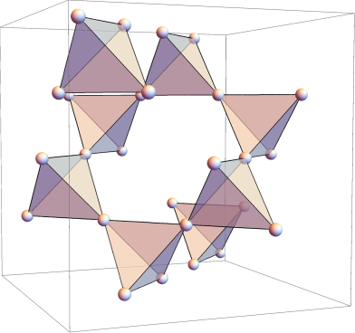
Figure 1: (Color online.) The illustration of the pyrochlore lattice, which is a three-dimensional network of corner-sharing tetrahedra.

It is well known that Monte Carlo simulation is a standard method to study statistical physics of many-body problems [8]. The single spin flip Metropolis method [9] is a robust algorithm for a wide range of subjects, but often suffers from the problem of slow dynamics; that is, it takes a long time for equilibration, for example, at temperatures near the critical temperature of the phase transition. To conquer the problem of slow dynamics, the cluster spin flip algorithms of Monte Carlo simulation have been proposed. The multi-cluster spin flip algorithm due to Swendsen and Wang (SW) [10] and the single-cluster spin flip algorithm due to Wolff [11] are typical examples.

For high-performance computing, the use of graphic processing unit (GPU) is a hot topic in computer science. The parallelization of cluster spin flip algorithm is not straightforward because the cluster labeling part of the cluster spin flip algorithm basically requires a sequential calculation, which is in contrast to the local calculation for the single spin flip algorithm. Komura and Okabe [12] proposed the GPU computing for the SW multi-cluster spin flip algorithm, where the ideas of Hawick et al. [13] and Kalentev et al. [14] were used in the cluster labeling part. Recently, Komura [15] proposed a refined version of the SW multi-cluster spin flip algorithm with a single GPU. Sample programs of the methods of Refs. [12] and [15] were published [16, 17]. As applications, the large-scale Monte Carlo study of the two-dimensional XY model [18], and the phase transitions of the Ising model on the Penrose lattice (quasicrystal) [19] were studied.

In this paper, we perform the high-performance computation of the ferromagnetic Ising model on the pyrochlore lattice. We use the GPU algorithm by Komura [15] for the SW method. We determine the critical temperature accurately based on the finite-size scaling (FSS) [20] of the Binder ratio [21]. Comparing with the data on the simple cubic lattice, we argue the universal FSS [22, 23]. We also calculate the classical XY model and the classical Heisenberg model on the pyrochlore lattice.

The remaining part of the paper is organized as follows: The model and the method are described in Sec. 2. The results are presented and discussed in Sec. 3, while Sec. 4 is devoted to the concluding remark.

2 Model and Simulation Method

We deal with the classical spin models on the pyrochlore lattice. For the simulation, we use the 16-site cubic unit cell of the pyrochlore lattice [27], and the systems with $L\times L\times L$ unit cells with periodic boundary conditions are treated. We made simulations for the system sizes up to $L$ =96; the numbers of sites are $N$ (=$16L^{3}$) = 14155776.

The Hamiltonian of the classical spin models is given by

$$\mathcal{H}=-J\sum_{\langle i,j\rangle}\bm{s}_{i}\cdot\bm{s}_{j},$$ (1)

where $J$ is the coupling and $\bm{s}_{i}$ is an $n$-dimensional unit vector on the lattice site $i$; $n$=1, 2, and 3 correspond to the Ising model, the classical XY model, and the classical Heisenberg model, respectively. The summation is taken over the nearest-neighbor pairs $\langle i,j\rangle$. We note that the coordination number of the pyrochlore lattice is six, which is the same as the simple cubic lattice.

We use the SW multi-cluster spin flip algorithm with a single GPU in the program of Ref. [15, 17]. The embedded cluster idea of Wolff [11] is used for simulating the spin systems with continuous symmetry (XY model and Heisenberg model). Once we have the table which gives the nearest-neighbor sites for each site, we can use the CUDA program of Ref. [15, 17]. The performance of the parallel computation with using the CUDA program was discussed in Ref. [15, 17]. The system sizes we treat are $L$ = 32 ($N$ = 524288), $L$ = 48 ($N$ = 1769472), $L$ = 64 ($N$ = 4194304), and $L$ = 96 ($N$ = 14155776). We discarded the first 10,000 Monte Carlo Steps (MCSs) to avoid the effects of initial configurations, and the next 200,000 MCSs were used for measurement. We made five independent runs for each size; the average was taken over five runs, and the statistical errors were estimated.

3 Results

3.1 Ising model

We start with the Ising model on the pyrochlore lattice. This model undergoes a second-order phase transition. To study the critical phenomena of second-order phase transition, it is convenient to calculate the moment ratio of the magnetization $M$ [21]. In Fig. 2, we plot the temperature dependence of the moment ratio of the magnetization $M$;

$$U(T)=\frac{\langle M(T)^{4}\rangle}{\langle M(T)^{2}\rangle^{2}}=\frac{\langle m(T)^{4}\rangle}{\langle m(T)^{2}\rangle^{2}}$$ (2)

with $m=M/N$, which is essentially the Binder ratio [21] except for the normalization. The value of $U(T)$ becomes 1 for $T\to 0$, whereas it becomes 3 for $T\to\infty$. In the high temperature limit the fluctuations become Gaussian, and a simple calculation yields $U(T)\to(n+2)/n$. The system sizes are $L=32\ (N=524288)$, $L=48\ (N=1769472)$, $L=64\ (N=4194304)$, and $L=96\ (N=14155776)$. The temperature is measured in units of $J$; in other words, we take $J=1$. The error bars are within the size of marks. We only show the data near the second-order phase transition. We see from Fig. 2 that the data with different $L$ cross around $T=4.214$, which yields the critical temperature $T_{c}$.

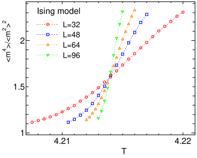
Figure 2: (Color online.) The moment ratio of the Ising model on the pyrochlore lattice. The system sizes are $L=32\ (N=524288)$, $L=48\ (N=1769472)$, $L=64\ (N=4194304)$, and $L=96\ (N=14155776)$.

To get precise estimate of $T_{c}$, let us consider the FSS [20] of the moment ratio $U(T)$. The FSS of $U(T)$ is expected to take a form

$$U(t)=f_{1}\Big{(}t\,(N^{1/3})^{1/\nu}\Big{)},$$ (3)

where $t=(T-T_{c})/T_{c}$, and $\nu$ is the critical exponent for the correlation length. We plot $U(T)=\langle m^{4}\rangle/\langle m^{2}\rangle^{2}$ as a function of $t(N^{1/3})^{1/\nu}$ in Fig. 3; all the data with different sizes are collapsed on a single curve within statistical errors. As for the linear size, we use $N^{1/3}=16^{1/3}L$ for a later convenience of the discussion of universal FSS. Here, the best choices of $T_{c}$ and $\nu$ are 4.21394(2) and 0.629(2), respectively. The estimated critical exponent $\nu$ is a universal one of the three-dimensional (3D) Ising exponent [28]. The estimated $T_{c}$, 4.21394(2), is about 93.4% of $T_{c}$ of the simple cubic lattice, 4.511524(20) (Ref. [28]), although the coordination number of both lattices is the same, that is, six.

We also consider the FSS of the magnetization. The FSS form of the squared magnetization is

$$\langle m^{2}\rangle=(N^{1/3})^{-2\beta/\nu}f_{2}\Big{(}t\,(N^{1/3})^{1/\nu}\Big{)},$$ (4)

where $\beta$ is the critical exponent for the magnetization. In Fig. 4, we give the FSS plot of the second moment of the magnetization of the Ising model on the pyrochlore lattice. We use the same $T_{c}$ and $\nu$ as the FSS plot of the moment ratio, and the best choice of $\beta/\nu$ is 0.520(5). We see that the FSS works very well.

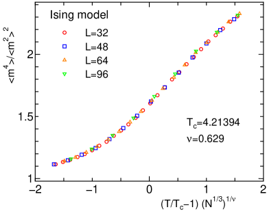
Figure 3: (Color online.) The FSS plot of the moment ratio of the Ising model on the pyrochlore lattice. The system size $N$ is $16L^{3}$. The choices of $T_{c}$ and $\nu$ are given in the figure.

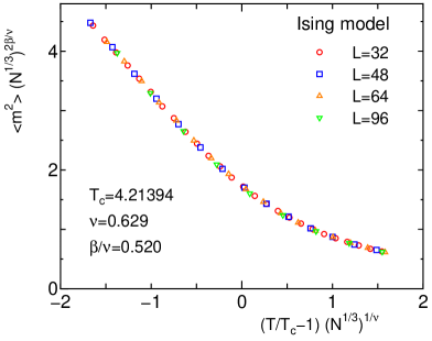
Figure 4: (Color online.) The FSS plot of the squared magnetization of the Ising model on the pyrochlore lattice. The system size $N$ is $16L^{3}$. The choices of $T_{c}$, $\nu$, and $\beta/\nu$ are given in the figure.

3.2 XY model

We turn to the classical XY model on the pyrochlore lattice. The temperature dependence of the moment ratio of the classical XY model on the pyrochlore lattice is plotted in Fig. 5. In the case of the XY model ($n=2$), $U(T)$ becomes 2 for $T\to\infty$. The system sizes are the same as the case of the Ising model. The error bars are within the size of marks. We see from the figure that the data with different $L$ cross around $T=2.029$.

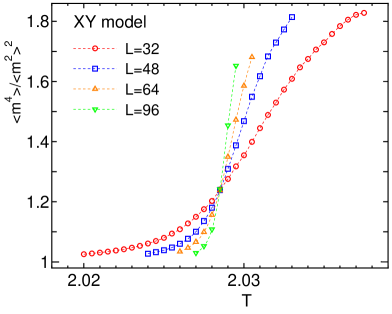
Figure 5: (Color online.) The moment ratio of the XY model on the pyrochlore lattice. The system sizes are $L=32\ (N=524288)$, $L=48\ (N=1769472)$, $L=64\ (N=4194304)$, and $L=96\ (N=14155776)$.

In Fig. 6, we give the FSS plot of the moment ratio of the classical XY model on the pyrochlore lattice. The data collapsing of different sizes is very good again. The best choices of $T_{c}$ and $\nu$ are 2.02850(2) and 0.672(2), respectively. The estimated critical exponent $\nu$ is a universal one of the 3D XY exponent [29]. The estimated $T_{c}$, 2.02850(2), is about 92.1% of $T_{c}$ of the simple cubic lattice, 2.20182(5) (Ref. [30]).

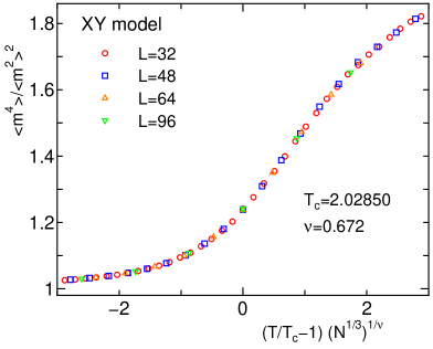
Figure 6: (Color online.) The FSS plot of the moment ratio of the XY model on the pyrochlore lattice. The system size $N$ is $16L^{3}$. The choices of $T_{c}$ and $\nu$ are given in the figure.

The FSS plot of the second moment of the magnetization of the classical XY model on the pyrochlore lattice is shown in Fig. 7. We use the same $T_{c}$ and $\nu$ as the FSS plot of the moment ratio, and the best choice of $\beta/\nu$ is 0.515(5).

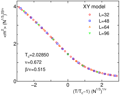
Figure 7: (Color online.) The FSS plot of the squared magnetization of the XY model on the pyrochlore lattice. The system size $N$ is $16L^{3}$. The choices of $T_{c}$, $\nu$, and $\beta/\nu$ are given in the figure.

3.3 Heisenberg model

Next, we consider the classical Heisenberg model on the pyrochlore lattice. In Fig. 8, we plot the temperature dependence of the moment ratio of the classical Heisenberg model on the pyrochlore lattice. In the case of Heisenberg model ($n=3$), $U(T)$ becomes 5/3 for $T\to\infty$.

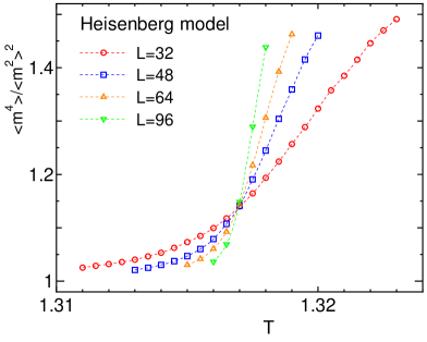
Figure 8: (Color online.) The moment ratio of the Heisenberg model on the pyrochlore lattice. The system sizes are $L=32\ (N=524288)$, $L=48\ (N=1769472)$, $L=64\ (N=4194304)$, and $L=96\ (N=14155776)$.

In Fig. 9, we show the FSS plot of the moment ratio of the classical Heisenberg model on the pyrochlore lattice. The data collapsing of different sizes is very good again. The best choices of $T_{c}$ and $\nu$ are 1.31695(2) and 0.711(2), respectively. The estimated critical exponent $\nu$ is a universal one of the 3D Heisenberg exponent [31]. The estimated $T_{c}$, 1.31695(2), is about 91.3% of $T_{c}$ of the simple cubic lattice, 1.4430(2) (Ref. [32]).

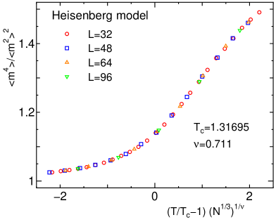
Figure 9: (Color online.) The FSS plot of the moment ratio of the Heisenberg model on the pyrochlore lattice. The system size $N$ is $16L^{3}$. The choices of $T_{c}$ and $\nu$ are given in the figure.

The FSS plot of the second moment of the magnetization of the classical Heisenberg model on the pyrochlore lattice is given in Fig. 10. We use the same $T_{c}$ and $\nu$ as the FSS plot of the moment ratio, and the best choice of $\beta/\nu$ is 0.515(5).

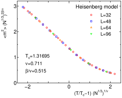
Figure 10: (Color online.) The FSS plot of the squared magnetization of the Heisenberg model on the pyrochlore lattice. The system size $N$ is $16L^{3}$. The choices of $T_{c}$, $\nu$, and $\beta/\nu$ are given in the figure.

3.4 Universal finite-size scaling

The idea of universal FSS functions was reported for critical phenomena in geometric percolation models [22]. Hu, Lin, and Chen [22] applied a histogram Monte Carlo simulation method to calculate the existence probability $E_{p}$ and the percolation probability $P$ of site and bond percolation on finite square, plane triangular, and honeycomb lattices, whose aspect ratios approximately have the relative proportions $1:\sqrt{3}/2:\sqrt{3}$. They found that the six percolation models have very nice universal FSS for $E_{p}$ and $P$ near the critical points of the percolation models with using nonuniversal metric factors. Using Monte Carlo simulation, Okabe and Kikuchi [23] found universal FSS for the Binder ratio [21] and magnetization distribution functions $p(m)$ of the Ising model on planar lattices. The universal FSS was further discussed in connection with spin models [24, 25, 26].

Here, we check the universal FSS for the classical spin systems on the pyrochlore lattice and on the simple cubic lattice. The FSS function for the Binder ratio, Eq. (3), and that for the magnetization, Eq. (4), may take the universal FSS forms such as

$$U(T)=\frac{\langle m(T)^{4}\rangle}{\langle m(T)^{2}\rangle^{2}}=f_{1}(D_{1}t(N^{1/3})^{1/\nu}),$$ (5)

$$\langle m^{2}\rangle=D_{2}(N^{1/3})^{-2\beta/\nu}f_{2}(D_{1}t(N^{1/3})^{1/\nu})$$ (6)

with nonuniversal metric factors $D_{1}$ and $D_{2}$.

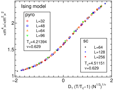
Figure 11: (Color online.) The universal FSS plot of the moment ratio of the Ising model. The system size $N$ is $16L^{3}$ for the pyrochlore lattice, whereas it is $L^{3}$ for the simple cubic lattice. The choices of $T_{c}$ and $\nu$ are given in the figure. The nonuniversal metric factor $D_{1}$ is chosen as 1.0 for the simple cubic lattice. The estimated $D_{1}$ for the pyrochlore lattice is 1.0.

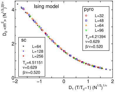
Figure 12: (Color online.) The universal FSS plot of the squared magnetization of the Ising model. The system size $N$ is $16L^{3}$ for the pyrochlore lattice, whereas it is $L^{3}$ for the simple cubic lattice. The choices of $T_{c}$, $\nu$, and $\beta/\nu$ are given in the figure. The nonuniversal metric factors $D_{1}$ and $D_{2}$ are chosen as 1.0 for the simple cubic lattice. The estimated $D_{1}$ and $D_{2}$ for the pyrochlore lattice are 1.0 and 0.91, respectively.

We show the universal FSS plot of the moment ratio of the Ising model on the pyrochlore lattice and the simple cubic lattice in Fig. 11. The system size $N$ is $L^{3}$ with the linear size $L$ for the simple cubic lattice. The metric factor for the simple cubic lattice is chosen as 1.0. The estimated metric factor $D_{1}$ for the pyrochlore lattice is 1.0. We find that the universal FSS plot works very well. The universal FSS plot of the squared magnetization of the Ising model on the pyrochlore lattice and the simple cubic lattice is given in Fig. 12. The estimated another metric factor $D_{2}$ is 0.91.

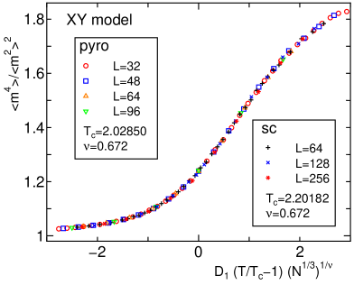
Figure 13: (Color online.) The universal FSS plot of the moment ratio of the XY model. The system size $N$ is $16L^{3}$ for the pyrochlore lattice, whereas it is $L^{3}$ for the simple cubic lattice. The choices of $T_{c}$ and $\nu$ are given in the figure. The nonuniversal metric factor $D_{1}$ is chosen as 1.0 for the simple cubic lattice. The estimated $D_{1}$ for the pyrochlore lattice is 0.96.

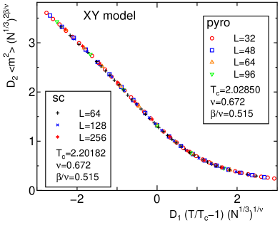
Figure 14: (Color online.) The universal FSS plot of the squared magnetization of the XY model. The system size $N$ is $16L^{3}$ for the pyrochlore lattice, whereas it is $L^{3}$ for the simple cubic lattice. The choices of $T_{c}$, $\nu$, and $\beta/\nu$ are given in the figure. The nonuniversal metric factors $D_{1}$ and $D_{2}$ are chosen as 1.0 for the simple cubic lattice. The estimated $D_{1}$ and $D_{2}$ for the pyrochlore lattice are 0.96 and 0.91, respectively.

The universal FSS plots of the moment ratio and of the squared magnetization of the XY model are shown in Figs. 13 and 14, respectively. The nonuniversal metric factors of the pyrochlore lattice are $D_{1}=0.96$ and $D_{2}=0.91$.

We also give the universal FSS plots of the moment ratio and of the squared magnetization of the Heisenberg model in Figs. 15 and 16, respectively. The nonuniversal metric factors of the pyrochlore lattice are $D_{1}=0.92$ and $D_{2}=0.91$.

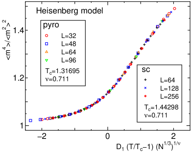
Figure 15: (Color online.) The universal FSS plot of the moment ratio of the Heisenberg model. The system size $N$ is $16L^{3}$ for the pyrochlore lattice, whereas it is $L^{3}$ for the simple cubic lattice. The choices of $T_{c}$ and $\nu$ are given in the figure. The nonuniversal metric factor $D_{1}$ is chosen as 1.0 for the simple cubic lattice. The estimated $D_{1}$ for the pyrochlore lattice is 0.92.

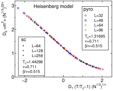
Figure 16: (Color online.) The universal FSS plot of the squared magnetization of the Heisenberg model. The system size $N$ is $16L^{3}$ for the pyrochlore lattice, whereas it is $L^{3}$ for the simple cubic lattice. The choices of $T_{c}$, $\nu$, and $\beta/\nu$ are given in the figure. The nonuniversal metric factors $D_{1}$ and $D_{2}$ are chosen as 1.0 for the simple cubic lattice. The estimated $D_{1}$ and $D_{2}$ for the pyrochlore lattice are 0.92 and 0.91, respectively.

4 Summary and Discussions

We have performed high-performance computation of the ferromagnetic classical spin models on the pyrochlore lattice. We have determined the critical temperature accurately based on the FSS of the Binder ratio. The estimated critical temperatures are 4.21394(2), 2.02850(2), and 1.31695(2) for the Ising model ($n=1$), the XY model ($n=2$), and the Heisenberg model ($n=3$), respectively. They are 93.4%, 92.1%, and 91.3% of $T_{c}$ of the simple cubic lattice, respectively. Estimated critical exponents are universal ones of the 3D values.

Comparing with the data on the simple cubic lattice, we have argued the universal FSS. We have obtained nice universal FSS plots by introducing nonuniversal metric factors $D_{1}$ and $D_{2}$. If we choose $D_{1}$ and $D_{2}$ as 1.0 for the simple cubic lattice, the nonuniversal metric factor $D_{1}$ for the pyrochlore is 1.0, 0.96, and 0.92 for the Ising model, the XY model, and the Heisenberg model, respectively; the nonuniversal metric factor $D_{2}$ is 0.91 for all the spin models.

In the present work, we have treated the perfect lattice. The extension to random systems, for example, a diluted system, is straightforward. It will be left to a future study.

We finally mention the algorithm of the present calculation. We have used the single-GPU-based SW multi-cluster spin flip algorithm [15] for large-scale simulations of spin models on the pyrochlore lattice. This algorithm can be adapted to a variety of lattices in a uniform fashion so long as a nearest-neighbor table is supplied. We have again confirmed the efficiency of the algorithm.

References

- [1] H.E. Stanley, Introduction to Phase Transitions and Critical Phenomena, Oxford Univ. Press, New York, 1971.
- [2] C.-K. Hu, Chinese J. Phys. 52 (2014) 1.
- [3] M.J. Harris, S.T. Bramwell, D.F. McMorrow, T. Zeiske, K.W. Godfrey, Phys. Rev. Lett. 79 (1997) 2554.
- [4] A.P. Ramirez, A. Hayashi, R.J. Cava, R. Siddharthan, B.S. Shastry, Nature (London) 399 (1999) 333.
- [5] S.T. Bramwell, J.P. Gingras, Science 294 (2001) 1495.
- [6] X. Ke, R.S. Freitas, B.G. Ueland, G.C. Lau, M.L. Dahlberg, R.J. Cava, R. Moessner, P. Schiffer, Phys. Rev. Lett. 99 (2007) 137203.
- [7] Y. Shevchenko, K. Nefedev, Y. Okabe, unpublished.
- [8] D.P. Landau, K. Binder, A Guide to Monte Carlo Simulations in Statistical Physics, 3rd edition, Cambridge University Press, Cambridge, 2009.
- [9] N. Metropolis, A.W. Rosenbluth, M.N. Rosenbluth, A.H. Teller, E. Teller, J. Chem. Phys. 21 (1953) 1087.
- [10] R.H. Swendsen, J.S. Wang, Phys. Rev. Lett. 58 (1987) 86.
- [11] U. Wolff, Phys. Rev. Lett. 62 (1989) 361.
- [12] Y. Komura, Y. Okabe, Comput. Phys. Comm. 183 (2012) 1155.
- [13] K.A. Hawick, A. Leist, D.P. Playne, Parallel Computing 36 (2010) 655.
- [14] O. Kalentev, A. Rai, S. Kemnitzb, R. Schneider, J. Parallel Distrib. Comput. 71 (2011) 615.
- [15] Y. Komura, Comput. Phys. Comm. 194 (2015) 54; arxiv:1603.08357 (2016).
- [16] Y. Komura, Y. Okabe, Comput. Phys. Comm. 185 (2014) 1038.
- [17] Y. Komura, Y. Okabe, Comput. Phys. Comm. 200 (2016) 400.
- [18] Y. Komura, Y. Okabe, J. Phys. Soc. Jpn. 81 (2012) 113001.
- [19] Y. Komura, Y. Okabe, J. Phys. Soc. Jpn. 85 (2016) 044004.
- [20] M.E. Fisher, in Proc. 1970 E. Fermi Int. School of Physics, edited by M. S. Green, Academic, New York, 1971, Vol. 51, pp. 1-99.
- [21] K. Binder, Z. Phys. B: Condens. Matter 43 (1981) 119.
- [22] C.-K. Hu, C.-Y. Lin, J.-A. Chen, Phys. Rev. Lett. 75 (1995) 193.
- [23] Y. Okabe, M. Kikuchi, Int. J. Mod. Phys. C 7 (1996) 287.
- [24] Y. Okabe, K. Kaneda, M. Kikuchi, C.-K. Hu, Phys. Rev. E 59 (1999) 1585.
- [25] Y. Tomita, Y. Okabe, C.-K. Hu, Phys. Rev. E 60 (1999) 2716.
- [26] M.-C. Wu, C.-K. Hu, N. Sh. Izmailian, Phys. Rev. E 67 (2003) 065103(R).
- [27] H. Shinaoka, Y. Tomita, Y. Motome, Phys. Rev. B 90 (2014) 165119.
- [28] H.W.J. Blöte, E. Luijten, J.R. Heringa, J. Phys. A: Math. Gen. 28 (1995) 6289.
- [29] M. Campostrini, M. Hasenbusch, A. Pelissetto, P. Rossi, E. Vicari, Phys. Rev. B 63 (2001) 214503.
- [30] A.P. Gottlob, M. Hasenbusch, S. Meyer, Nucl. Phys. B (Proc. Suppl.) 30 (1993) 838.
- [31] M. Campostrini, M. Hasenbusch, A. Pelissetto, P. Rossi, E. Vicari, Phys. Rev. B 65 (2002) 144520.
- [32] C. Holm, W. Janke, Phys. Rev. B 48 (1993) 936.