Instrumental Variable Quantile Regression with Misclassification

Abstract

This paper investigates the instrumental variable quantile regression model (Chernozhukov and Hansen, 2005, 2013) with a binary endogenous treatment. It offers two identification results when the treatment status is not directly observed. The first result is that, remarkably, the reduced-form quantile regression of the outcome variable on the instrumental variable provides a lower bound on the structural quantile treatment effect under the stochastic monotonicity condition (Small and Tan, 2007; DiNardo and Lee, 2011). This result is relevant, not only when the treatment variable is subject to misclassification, but also when any measurement of the treatment variable is not available. The second result is for the structural quantile function when the treatment status is measured with error; the sharp identified set is characterized by a set of moment conditions under widely-used assumptions on the measurement error. Furthermore, an inference method is provided in the presence of other covariates.

Keywords: Misclassification; Instrumental variable quantile regression; Partial identification; Binary endogenous treatment

1 Introduction

The instrumental variable quantile regression model (Chernozhukov and Hansen, 2005, 2013) aims to investigate heterogeneous treatment effects in the presence of an endogenous binary treatment variable. In many empirical applications, the treatment variable is potentially mismeasured, so it is empirically relevant how researchers can use the instrumental variable quantile regression model with a mismeasured treatment variable. For example, Chernozhukov and Hansen (2004) use the instrumental variable quantile regression model to investigate the quantile treatment effect of 401(k) participation on saving behaviors, but the pension plan type is subject to measurement error in survey datasets. Using the Health and Retirement Study, Gustman et al. (2008) estimate that around one-fourth of the survey respondents misclassified their pension plan type. To the best of my knowledge, however, no paper has investigated the instrumental variable quantile regression model when a binary regressor is potentially misclassified and endogenous.

This paper has two identification results on the structural quantile function under the rank similarity condition. The first identification result considers a reduced-form parameter, that is, the coefficient of the instrumental variable when running the quantile regression of the outcome variable on the instrumental variable. Under the rank similarity condition and the stochastic monotonicity condition (Small and Tan, 2007; DiNardo and Lee, 2011), this reduced-form parameter can be used as a lower bound for the structural quantile treatment effect. Although it has been used by empirical studies (e.g., Bitler et al., 2016), the reduced-form quantile regression on the instrumental variable has not been formally related to the structural quantile treatment effect. Moreover, this result does not depend on the treatment variable or its measurement, and therefore it is relevant even when a measurement does not exist.

The second identification result is to derive moment conditions for the structural quantile function when the treatment variable is measured with exogenous errors. The exogeneity of the measurement error is widely assumed in the measurement error literature (e.g., Bound et al., 2001) and yields exclusion restrictions similar to Henry et al. (2014). Given the structure of the moment conditions, the structural quantile function can be under-identified even if the order condition for point identification holds. In other words, additional assumptions or variables are necessary to achieve point identification for the structural quantile function. As an example of additional restrictions, this paper considers two observed measurements for one latent treatment variable, and point-identify the structural quantile function. Point identification results from combining two existing methods: misclassification correction techniques (Mahajan, 2006; Lewbel, 2007; Hu, 2008), and the identification results in Chernozhukov and Hansen (2005, 2013).

Based on the partial identification result, an inference method for the structural quantile function is provided by incorporating the misclassification probabilities in the inference method of Chernozhukov and Hansen (2008). The proposed inference method can include covariates other than the treatment variable, and it is computationally feasible by imposing a linear-in-parameters structure on the structural quantile function. Simulation studies and an empirical illustration demonstrate the finite sample performance for the proposed inference method.

Related to this paper, several papers have considered the problem of mis-measured regressors in the quantile regression framework, e.g., Chesher (1991, 2017), Schennach (2008), Galvao and Montes-Rojas (2009), Wei and Carroll (2009), Firpo et al. (2017), and Song (2018). They focus on the case in which the mismeasured regressor is continuously distributed, whereas this paper focuses on a binary treatment variable in which the measurement error has to be nonclassical.

Mahajan (2006), Lewbel (2007), and Hu (2008) consider identification of the average treatment effect (or, more generally, the conditional density function of the outcome variable given the true treatment variable) when a discrete treatment variable is mismeasured. Their identification strategy is based on the assumption that the true treatment variable (or the individual treatment effect in Lewbel, 2007) is exogenous, and there is no straightforward way to modify their results to the endogenous treatment.

Calvi et al. (2017); Yanagi (2019); Ura (2018) investigate the local average treatment effect model with a mismeasured binary treatment. The local average treatment effect model is also a model for heterogeneous treatment effects in the presence of endogeneity but has a different structure than the instrumental variable quantile regression model.

Frazis and Loewenstein (2003), DiTraglia and García-Jimeno (2019) and Nguimkeu et al. (2019) study a linear regression model in which a binary regressor is potentially misclassified and endogenous. Their approach is based on a homogenous treatment effect, which does not hold in the quantile treatment effect framework.

The remainder of this paper is organized as follows. Section 2 introduces the instrumental variable quantile regression model (Chernozhukov and Hansen, 2005, 2013) with a misclassified treatment variable. Section 3 studies the reduced-form quantile regression of the outcome variable on the instrumental variable. Section 4 presents the identified set for the structural quantile function. Section 5 proposes an inference method based on the identification analysis in Section 4. Section 6 provides an empirical illustration and simulation studies. Section 7 concludes. The appendix includes the proofs and additional results.

The rest of this paper uses the following notations. $Pr$ denotes the true probability measure for the observed and unobserved random variables. $Q_{RV_{1}\mid RV_{2}}(\tau)$ is the $\tau$-th conditional quantile of a continuous random variable $RV_{1}$ given a random variable $RV_{2}$. $F_{RV_{1}\mid RV_{2}}$ is the conditional cumulative distribution function of a random variable $RV_{1}$ given a random variable $RV_{2}$. $f_{RV_{1}\mid RV_{2}}$ is the conditional probability density function of a random variable $RV_{1}$ given a random variable $RV_{2}$.

2 Instrumental variable quantile regression model with misclassification

This section presents notations and assumptions that are essentially those of the instrumental variable quantile regression model (Chernozhukov and Hansen, 2005, 2013), though the treatment variable $D^{\ast}$ is not observed in this paper. For the sake of simplicity, covariates are omitted other than the treatment variable when analyzing the identification problem. In the instrumental variable quantile regression model, $Y$ is an outcome variable, $D^{\ast}$ is a binary (true but latent) treatment variable taking values in $\{0,1\}$, and $Z$ is an instrumental variable. $D^{\ast}=1$ means that the individual is treated; otherwise, $D^{\ast}=0$.

In Chernozhukov and Hansen (2004) and Section 6.1 of this paper, the outcome variable $Y$ is the net amount of financial assets in dollars, the treatment variable $D^{\ast}$ is the participation status in a 401(k) program, and the instrumental variable $Z$ is the 401(k) eligibility indicator of whether an employer offers a 401(k) program to employees.

The goal of this paper is to investigate treatment effects of $D^{\ast}$ on $Y$. The error term $(U_{0},U_{1})$ and the (unknown) structural quantile function $q(d^{\ast},u)$ are used to model the relationship between the outcome variable $Y$ and the binary treatment variable $D^{\ast}$:

$$Y=q(D^{\ast},U)\mbox{ where }U=(1-D^{\ast})U_{0}+D^{\ast}U_{1}.$$

The random variable $q(d^{\ast},U_{d^{\ast}})$ is the potential outcome variable when $D^{\ast}=d^{\ast}$. The parameter of interest is the $\tau$-th quantile of the counterfactual outcome variable, $q(d^{\ast},\tau)$, for a given value of $\tau\in(0,1)$.

To identify $q(d^{\ast},u)$ even partially, it is necessary to impose some structure on the unknown function, $q(d^{\ast},u)$, and on the unobserved variable, $U_{d^{\ast}}$. The following assumptions are based on Chernozhukov and Hansen (2005, 2013). Unlike their papers, the condition is local at the given value of $\tau$, which is sufficient for deriving the testable implication in Chernozhukov and Hansen (2005, Theorem 1) for the structural quantile function at $\tau$.

Assumption 1.

The mapping $u\mapsto q(d^{\ast},u)$ is strictly increasing and left-continuous for every $u\in[0,1]$, and has the inverse $y\mapsto q^{-1}(y,d^{\ast})$.

Assumption 2.

(i) $Pr(U_{0}\leq\tau\mid Z)=Pr(U_{1}\leq\tau\mid Z)=\tau$. (ii) $Pr(U_{0}\leq\tau\mid D^{\ast},Z)=Pr(U_{1}\leq\tau\mid D^{\ast},Z)$.

Assumption 1 requires that the outcome variable $Y$ is continuously distributed. Assumption 2 (i) is the exogeneity of the instrumental variable $Z$. This assumption allows for the endogeneity of the treatment variable $D^{\ast}$. Assumption 2 (ii) is the rank similarity condition on $U_{d^{\ast}}\leq\tau$. It is a relaxation of the rank invariance condition, $U_{0}=U_{1}$, that an individual’s rank, $U_{d^{\ast}}$, is the same regardless of whether the individual is treated or controlled. The rank similarity condition allows the two unobserved heterogeneity terms, $U_{1}$ and $U_{0}$, to be different, though it still requires them to have the same distribution given the endogenous treatment assignment and the instrumental variable. It enables the $\tau$-th quantile of the counterfactual outcome variable, $q(d^{\ast},\tau)$, to be compared between the control group ($d^{\ast}=0$) and the treatment group ($d^{\ast}=1$). The rank similarity condition is a restriction on the unobserved heterogeneity in the outcome variable equation and has been widely used for investigating heterogenous treatment effects (e.g., Doksum, 1974; Heckman et al., 1997; Chernozhukov and Hansen, 2004).

Under the rank similarity condition, Chernozhukov and Hansen (2005) obtain the following relationship between the distribution of $(Y,D^{\ast},Z)$ and the structural quantile function $q(d^{\ast},\tau)$.

Lemma 1 (Chernozhukov and Hansen, 2005, Theorem 1).

Under Assumptions 1 and 2,

$$Pr(U\leq\tau\mid Z)=\tau\mbox{ and }Pr(Y\leq q(D^{\ast},\tau)\mid Z)=\tau.$$ (1)

The rest of this paper adds the complication that the binary treatment variable $D^{\ast}$ may not be observed. Then the equality (1) cannot be directly used for identifying the structural quantile function.

3 Quantile regression of $Y$ on $Z$

This section does not use any measurement of $D^{\ast}$; instead the relationship between the outcome variable $Y$ and the instrumental variable $Z$ is used to provide a lower bound on the structural quantile treatment effect $q(1,\tau)-q(0,\tau)$. Namely, $Q_{Y\mid Z=z_{1}}(\tau)-Q_{Y\mid Z=z_{0}}(\tau)$ can be a lower bound on $q(1,\tau)-q(0,\tau)$, when $Z$ is a binary variable taking $z_{0}$ and $z_{1}$. This analysis provides a new structural interpretation to $Q_{Y\mid Z=z_{1}}(\tau)-Q_{Y\mid Z=z_{0}}(\tau)$, which is computed as the regression coefficient from the quantile regression of $Y$ on $Z$. When $Z$ takes more than two values, the discussion in this section can be applied by selecting any two values in the support of $Z$ or partitioning the support into two parts. It is worth clarifying that the results in this section and the following sections are valid regardless of whether $Z$ is binary, discrete, continuous, or mixed.

The result in this section uses the stochastic monotonicity condition (Small and Tan, 2007 and DiNardo and Lee, 2011). It assumes a positive relationship between the treatment variable $D^{\ast}$ and the instrumental variable $Z$ in which, for every possible realization $u$ of $U$, the probability of being treated $f_{U_{1},D^{\ast}\mid Z=z}(u,1)$ is weakly increasing in $z$, and the probability of being untreated $f_{U_{0},D^{\ast}\mid Z=z}(u,0)$ is weakly decreasing in $z$. The condition is weaker than the deterministic monotonicity condition (Imbens and Angrist, 1994; Angrist et al., 1996) because it allows for defiers, i.e., some individuals who change $D^{\ast}$ from $1$ to $0$ when $Z$ increases.

Definition 1.

The stochastic monotonicity condition is that

$$f_{U_{0},D^{\ast}\mid Z=z_{1}}(u,0)\leq f_{U_{0},D^{\ast}\mid Z=z_{0}}(u,0)\mbox{ and }f_{U_{1},D^{\ast}\mid Z=z_{1}}(u,1)\geq f_{U_{1},D^{\ast}\mid Z=z_{0}}(u,1)$$ (2)

for every $u\in[0,1]$.

Theorem 1 shows that, under the stochastic monotonicity condition in (2), $Q_{Y\mid Z=z_{1}}(\tau)-Q_{Y\mid Z=z_{0}}(\tau)$ is biased towards zero compared to the structural quantile treatment effect $q(1,\tau)-q(0,\tau)$.

Theorem 1.

Suppose that Assumptions 1 and 2 hold and that the stochastic monotonicity condition holds.

1. There is some unknown constant $\kappa\in[0,1]$ such that

   $$Q_{Y\mid Z=z_{1}}(\tau)-Q_{Y\mid Z=z_{0}}(\tau)=\kappa\times(q(1,\tau)-q(0,\tau)).$$ (3)

2. If $f_{U_{0},D^{\ast}\mid Z=z_{1}}(u,0)<f_{U_{0},D^{\ast}\mid Z=z_{0}}(u,0)$ and $f_{U_{1},D^{\ast}\mid Z=z_{1}}(u,1)>f_{U_{1},D^{\ast}\mid Z=z_{0}}(u,1)$ in a neighborhood of $\tau$, then $\kappa\neq 0$.

This theorem provides a one-sided bound on $q(1,\tau)-q(0,\tau)$: $q(1,\tau)-q(0,\tau)\geq Q_{Y\mid Z=z_{1}}(\tau)-Q_{Y\mid Z=z_{0}}(\tau)$ if $Q_{Y\mid Z=z_{1}}(\tau)-Q_{Y\mid Z=z_{0}}(\tau)\geq 0$; and $q(1,\tau)-q(0,\tau)\leq Q_{Y\mid Z=z_{1}}(\tau)-Q_{Y\mid Z=z_{0}}(\tau)$ if $Q_{Y\mid Z=z_{1}}(\tau)-Q_{Y\mid Z=z_{0}}(\tau)\leq 0$. This bound gives researchers a justification for using $Q_{Y\mid Z=z_{1}}(\tau)-Q_{Y\mid Z=z_{0}}(\tau)$, which is a lower bound for the structural quantile treatment effect. Note that $Q_{Y\mid Z=z_{1}}(\tau)-Q_{Y\mid Z=z_{0}}(\tau)$ is a simple object to compute; it is obtained as the quantile regression coefficient on $Z$ and various statistical software packages include linear and nonlinear quantile regressions (e.g., the qreg command in Stata).

The stochastic monotonicity condition cannot be removed from Theorem 1, but Lemma 5 in the appendix shows that Eq. (3) holds with $\kappa\in[-1,1]$ even if the stochastic monotonicity condition does not hold. In other words, the inequality $|Q_{Y\mid Z=z_{1}}(\tau)-Q_{Y\mid Z=z_{0}}(\tau)|\leq|q(1,\tau)-q(0,\tau))|$ still holds without the stochastic monotonicity condition. It is possible to use this inequality to test the significance of $D^{\ast}$ by testing $Q_{Y\mid Z=z_{1}}(\tau)-Q_{Y\mid Z=z_{0}}(\tau)=0$.

4 Identified set for the structural quantile function

This section considers use of a potentially misclassified treatment variable $D$ and provides the sharp identified set for the structural quantile function $q(\cdot,\tau)$. To extract some information about the true treatment $D^{\ast}$ from its measurement $D$, the following restrictions on the misclassification probabilities are imposed.

Assumption 3.

(i) $(Pr(D=1\mid D^{\ast}=0,Y,Z),Pr(D=0\mid D^{\ast}=1,Y,Z))=(\pi_{0},\pi_{1})$ for some constants $(\pi_{0},\pi_{1})$. (ii) $Pr(D\neq D^{\ast}\mid D^{\ast}=0,Y,Z)+Pr(D\neq D^{\ast}\mid D^{\ast}=1,Y,Z)<1$.

Assumption 3 (i) is that the measurement error does not depend on $(Y,Z)$. Assumption 3 (ii) is that the measurement $D$ is positively correlated with the true treatment variable $D^{\ast}$. These assumptions are widely used in the literature on misclassification (e.g., Hausman et al., 1998, Mahajan, 2006; Lewbel, 2007; and Hu, 2008).

The sharp identified set for $q(\cdot,\tau)$ is the set of values for $q(\cdot,\tau)$ that exhausts all the information from the model and the data distribution. Let $\mathcal{Q}$ be a subset of the set of functions of $\{0,1\}\times[0,1]$ to $\mathbb{R}$, and $\mathcal{P}^{\ast}$ be a subset of the set of probability distributions for $(D,Z,U_{0},U_{1},D^{\ast})$. Given a distribution $P$ for $(Y,D,Z)$, the sharp identified set for $(q,P^{\ast})$ is the set of elements $(\tilde{q},\tilde{P}^{\ast})$ of $\mathcal{Q}\times\mathcal{P}^{\ast}$ such that $P$ is the distribution for $(\tilde{q}(D^{\ast},U),D,Z)$ under $\tilde{P}^{\ast}$. The sharp identified set for $q(\cdot,\tau)$ is defined as the projection of the sharp identified set for $(q,P^{\ast})$ on the component $q(\cdot,\tau)$.

The following theorem characterizes the sharp identified set for $q(\cdot,\tau)$ under Assumptions 1, 2, and 3, by using moment equalities and inequalities.

Theorem 2.

Assume that all the elements in $\mathcal{Q}\times\mathcal{P}^{\ast}$ satisfy Assumptions 1, 2, and 3. (a) Given a distribution $P$ for the observed variables, if $(y_{0},y_{1})$ belongs to the sharp identified set for $q(\cdot,\tau)$, then

$$P(Y\leq y_{D}\mid Z)-\tau=p_{1}(P(Y\leq y_{0}\mid Z)-\tau)+p_{0}(P(Y\leq y_{1}\mid Z)-\tau)$$ (4)

for some $(p_{0},p_{1})$ with $p_{0}+p_{1}<1$ such that

$$0\leq p_{0}\leq P(D=1\mid Y,Z)\mbox{ a.s.}\mbox{ and }0\leq p_{1}\leq P(D=0\mid Y,Z)\mbox{ a.s.}$$

(b) The converse is also true if $\mathcal{Q}\times\mathcal{P}^{\ast}$ includes all $(q,P^{\ast})$’s satisfying Assumptions 1, 2, and 3.

The moment equality condition in Eq. (4) is equivalent to the main testable implication in Chernozhukov and Hansen (2005) when $(p_{0},p_{1})=(\pi_{0},\pi_{1})$ where $(\pi_{0},\pi_{1})$ are the true unknown misclassification probabilities defined in Assumption 3. The moment inequality conditions about $(\pi_{0},\pi_{1})$ are derived from the following calculations:

$$Pr(D=1\mid Y,Z)=\pi_{0}+(1-\pi_{0}-\pi_{1})Pr(D^{\ast}=1\mid Y,Z)\geq\pi_{0}$$

$$Pr(D=0\mid Y,Z)=\pi_{1}+(1-\pi_{0}-\pi_{1})Pr(D^{\ast}=0\mid Y,Z)\geq\pi_{1}.$$

As a corollary to Theorem 2, it is possible to compare the identified set for $q(\cdot,\tau)$ and the estimand in Chernozhukov and Hansen (2005), which does not consider measurement error in $D$.

Corollary 1.

Suppose all the assumptions in Theorem 2 (b) hold. Every solution $(y_{0},y_{1})$ to $P(Y\leq y_{D}\mid Z)-\tau=0$, belongs to the sharp identified set for $q(\cdot,\tau)$.

As another corollary to Theorem 2, it is possible to relate $Q_{Y\mid Z}(\tau)$ to the identified set for $q(\cdot,\tau)$. Although $Q_{Y\mid Z=z_{1}}(\tau)-Q_{Y\mid Z=z_{0}}(\tau)$ can be used as a lower bound for $q(1,\tau)-q(0,\tau)$, it does not always belong to the identified set.

Corollary 2.

Consider two points, $z_{0}$ and $z_{1}$, in the support of $Z$, and suppose all the assumptions in Theorem 2 (b) hold. Then $(y_{0},y_{1})=(Q_{Y\mid Z=z_{0}}(\tau),Q_{Y\mid Z=z_{1}}(\tau))$ belongs to the sharp identified set for $q(\cdot,\tau)$ if and only if $P(D=1\mid\{y_{0}<Y\leq y_{1}\mbox{ or }y_{1}<Y\leq y_{0}\},Z=z_{0})\leq P(D=1\mid Y,Z)$ a.s. and $P(D=0\mid\{y_{0}<Y\leq y_{1}\mbox{ or }y_{1}<Y\leq y_{0}\},Z=z_{1})\leq P(D=0\mid Y,Z)$ a.s.

Note that, by the exogeneity of $Z$, $(q(0,\tau),q(1,\tau))=(Q_{Y\mid Z=z_{0}}(\tau),Q_{Y\mid Z=z_{1}}(\tau))$ if $D^{\ast}=1\{Z=z_{1}\}$. Corollary 2 is roughly related to the observation that, under Assumption 3, $D^{\ast}=1\{Z=z_{1}\}$ implies

$$P(D=1\mid\{y_{0}<Y\leq y_{1}\mbox{ or }y_{1}<Y\leq y_{0}\},Z=z_{0}) = P(D=1\mid\{y_{0}<Y\leq y_{1}\mbox{ or }y_{1}<Y\leq y_{0}\},D^{\ast}=0)$$

$$= \pi_{0}$$

$$\leq \pi_{0}+(1-\pi_{0}-\pi_{1})P(D^{\ast}=1\mid Y,Z)$$

$$= P(D=1\mid Y,Z)$$

$$P(D=0\mid\{y_{0}<Y\leq y_{1}\mbox{ or }y_{1}<Y\leq y_{0}\},Z=z_{1}) = P(D=0\mid\{y_{0}<Y\leq y_{1}\mbox{ or }y_{1}<Y\leq y_{0}\},D^{\ast}=1)$$

$$= \pi_{1}$$

$$\leq \pi_{1}+(1-\pi_{0}-\pi_{1})P(D^{\ast}=0\mid Y,Z)$$

$$= P(D=0\mid Y,Z).$$

The precise derivations are found in the proof in the Appendix.

4.1 Under-identification even with large variation in $Z$

This section shows that the structural quantile function is not point identified in general unless there is additional information on the model primitives $(q,P^{\ast})$. The failure of point identification is due to the rank condition and happens regardless of the order condition based on Eq. (4), where the number of the parameters is $4$, and the number of the equations is the number of the support points of $Z$. Theorem 3 presents this failure for a class of data generating processes. In particular, the theorem states that the quantile treatment effect can be under-identified if one cannot exclude that the treatment is exogenous. Based on the result, it is necessary to impose additional assumptions (other than the ones maintained in this paper) to achieve point identification when the treatment variable is potentially misclassified.

Theorem 3.

Consider $\bar{d}^{\ast}=0$ or $\bar{d}^{\ast}=1$. Assume (i) the mapping $u\mapsto q^{-1}(q(1,u),0)$ is Lipschitz continuous, (ii) $q(d^{\ast},\tau)\neq q(1-d^{\ast},\tau)$, (iii) $(U_{0},U_{1})$ is independent of $(D^{\ast},Z)$, (iv) $\pi_{\bar{d}^{\ast}}>0$, and (v) for sufficiently small $\varepsilon>0$, the following three statements holds:

1. $\tilde{q}\in\mathcal{Q}$ for every strictly increasing bijection $t$ of $[0,1]$ to $[0,1]$ such that $|t(u)-u|\leq\varepsilon$ for every $u\in(0,1)$, where $\tilde{q}(d^{\ast},\cdot)=q(d^{\ast},t(\cdot))$ and $\tilde{q}(1-d^{\ast},\cdot)=q(1-d^{\ast},\cdot)$.

2. $\tilde{P}^{\ast}\in\mathcal{P}^{\ast}$ for every distribution $\tilde{P}^{\ast}$ for $(D,Z,U_{0},U_{1},D^{\ast})$ such that $\tilde{P}^{\ast}$ satisfies Assumption 2 and that

   $$\tilde{P}^{\ast}(D=1-\bar{d}^{\ast}\mid U_{0},U_{1},D^{\ast}=\bar{d}^{\ast},Z)=\pi_{\bar{d}^{\ast}}-\varepsilon$$

   $$\tilde{P}^{\ast}(D=\bar{d}^{\ast}\mid U_{0},U_{1},D^{\ast}=1-\bar{d}^{\ast},Z)=\pi_{1-\bar{d}^{\ast}}$$

   $$|\tilde{P}^{\ast}(U_{0}\leq u_{0},U_{1}\leq u_{1},D^{\ast}=d^{\ast},Z\leq z)-{P}^{\ast}(U_{0}\leq u_{0},U_{1}\leq u_{1},D^{\ast}=d^{\ast},Z\leq z)|\leq\varepsilon.$$

Then the sharp identified set for $q(\cdot,\tau)$ has more than one element.

Condition (i) is a regularity condition. Condition (ii) is that the treatment variable can have a non-zero effect on the outcome variable at quantile index $\tau$. Condition (iii) is that the treatment variable can be exogenous. Condition (iv) is that there is a non-zero measurement error. Condition (v) is a condition about the size of the parameter space $\mathcal{Q}\times\mathcal{P}^{\ast}$. A sufficient condition for (v) is that $\mathcal{Q}\times\mathcal{P}^{\ast}$ includes all $(q,P^{\ast})$’s satisfying Assumptions 1, 2, and 3.

Condition (iii) needs a careful discussion. Theorem 3 states that the quantile treatment effect is not always point identified unless the treatment is assumed to be endogenous. This theorem is more relevant when one cannot exclude that $D^{\ast}$ is exogenous than when $D^{\ast}$ is known to be exogenous. When one cannot exclude that $D^{\ast}$ is exogenous, there is a possibility for the lack of point identification. It can be possible to point-identify the quantile treatment function if one can assume that $D^{\ast}$ is not exogenous.

4.2 Point identification with second measurement

Given the under-identification result in Theorem 3, this section considers the case of two measurements for $D^{\ast}$ to achieve point identification of the structural quantile function. The identification strategy is based on existing results in the econometric literature. First, the results in Mahajan (2006), Lewbel (2007), and Hu (2008) are applied to identify $f_{Y,D^{\ast}\mid Z}$. Given identification of $f_{Y,D^{\ast}\mid Z}$, the identification result in Chernozhukov and Hansen (2005, 2013) recovers the structural quantile function.

The following assumption and Lemma 2 are based on Theorem 1 in Hu (2008).

Assumption 4.

(i) The two measurements, $D$ and $V$, are conditionally independent given $D^{\ast}$. (ii) $0<f_{D^{\ast}\mid Z=z_{1}}(0)<1$. (iii) There are two points, $v_{0}$ and $v_{1}$, in the support of $V$ such that

$$\left(\begin{array}[]{cc}f_{V\mid D^{\ast}=0}(v_{0})&f_{V\mid D^{\ast}=0}(v_{1})\\ f_{V\mid D^{\ast}=1}(v_{0})&f_{V\mid D^{\ast}=1}(v_{1})\\ \end{array}\right)$$

is invertible. (iv) $P(D=D^{\ast}\mid D^{\ast})>1/2$. (v) There are two points, $z_{0}$ and $z_{1}$, in the support of $Z$.

Lemma 2.

Under Assumptions 3 and 4, $f_{(Y,D^{\ast})\mid Z}$ is point identified.

Chernozhukov and Hansen (2013) provide a simple sufficient condition for the the global identification of the structural quantile function given $f_{(Y,D^{\ast})\mid Z}$. The following assumption and identification result are borrowed from Chernozhukov and Hansen (2013, Section 3.1).

Assumption 5.

There is a cube $\mathcal{L}$ with $(q(0,\tau),q(1,\tau))\in\mathcal{L}$ such that

$$\frac{f_{(Y,D^{\ast})\mid Z=z_{1}}(y_{1},1)}{f_{(Y,D^{\ast})\mid Z=z_{1}}(y_{0},0)}>\frac{f_{(Y,D^{\ast})\mid Z=z_{0}}(y_{1},1)}{f_{(Y,D^{\ast})\mid Z=z_{0}}(y_{0},0)}\mbox{, }f_{(Y,D^{\ast})\mid Z=z_{1}}(y_{1},1)>0\mbox{ and }f_{(Y,D^{\ast})\mid Z=z_{0}}(y_{0},0)>0$$

for all $(y_{0},y_{1})\in\mathcal{L}$.

Lemma 3.

Under Assumptions 1, 2 and 5, $(q(0,\tau),q(1,\tau))$ is uniquely determined from $f_{(Y,D^{\ast})\mid Z}$.

By Lemmas 2 and 3, the structural quantile function can be identified with two measurements for $D^{\ast}$.

Theorem 4.

Under Assumptions 1, 2, 3, 4, and 5, $(q(0,\tau),q(1,\tau))$ is identified.

5 Inference procedure with covariates

This section proposes an inference method for the structural quantile function. The method extends the inference method in Chernozhukov and Hansen (2008) to incorporate misclassification probabilities. To include control variables $X$, a linear-in-parameters structure is imposed on the structural quantile function:

$$Y=q(D^{\ast},X,U)\mbox{ with }q(d^{\ast},x,\tau)=\alpha_{0}d^{\ast}+x^{\prime}\beta_{0}.$$ (5)

This section focuses on constructing a confidence interval for $\alpha_{0}$.

With control variables $X$, Assumptions 1-3 are modified into the following assumptions:

Assumption 6.

With probability one, the mapping $u\mapsto q(d^{\ast},X,u)$ is strictly increasing and left-continuous for every $u\in[0,1]$.

Assumption 7.

(i) $Pr(U_{0}\leq\tau\mid Z,X)=Pr(U_{1}\leq\tau\mid Z,X)=\tau$. (ii) $Pr(U_{0}\leq\tau\mid D^{\ast},Z,X)=Pr(U_{1}\leq\tau\mid D^{\ast},Z,X)$.

Assumption 8.

(i) For each $d^{\ast}=0,1$, $Pr(D\neq D^{\ast}\mid D^{\ast}=d^{\ast},Y,Z,X)$ is a constant, denoted by $\pi_{d^{\ast}}$. (ii) $Pr(D\neq D^{\ast}\mid D^{\ast}=0,Y,Z,X)+Pr(D\neq D^{\ast}\mid D^{\ast}=1,Y,Z,X)<1$.

Given $n$ i.i.d. copies $\{(Y_{i},D_{i},X_{i},Z_{i}):i=1,\ldots,n\}$ of $(Y,D,X,Z)$, a confidence interval for $\alpha_{0}$ is constructed via the following two steps. The first step constructs a confidence interval for $(\pi_{0},\pi_{1})$. Given each point in the confidence interval for $(\pi_{0},\pi_{1})$, the second step constructs a confidence interval for $\alpha_{0}$. The size control comes from the Bonferroni correction for the first and second steps.

The following condition is imposed on a $(1-\mathrm{size}_{1})$ confidence region, $CI_{1}$, for $(\pi_{0},\pi_{1})$.

Assumption 9.

$\liminf_{n\rightarrow\infty}Pr((\pi_{0},\pi_{1})\in CI_{1})\geq 1-\mathrm{size}_{1}$.

In the empirical illustration, $CI_{1}$ is constructed by inverting the one-tailed $t$-tests based on $\pi_{0}\leq E[D\mid Z=0]$ and $\pi_{1}\leq E[1-D\mid Z=1]$, where $\mathrm{size}_{1}/2$ for each $t$-test. In the empirical illustration, the confidence interval for $\alpha_{0}$ is bounded by using $E_{n}[D\mid Z=0]=0$ and $E_{n}[1-D\mid Z=1]\approx 0.3$.

At the true value $(\alpha_{0},\pi_{0},\pi_{1})$ of $(\alpha,p_{0},p_{1})$, the following testable implications (cf. Chernozhukov and Hansen, 2008) hold. As in Chernozhukov and Hansen (2008), it is possible to replace $Z$ with a function $g(X,Z)$ of $(X,Z)$.

Lemma 4.

Under Assumptions 6-8,

$$0\in\operatorname*{arg\,min}_{\gamma}\min_{\beta}Q_{0}(\theta;\alpha_{0},\pi_{0},\pi_{1}).$$

where $\nu_{0}(y,x,z)=E[D\mid Y=y,X=x,Z=z]$, $t_{+}=1\{t\geq 0\}\cdot t$, $\rho_{\tau}(t)=(\tau-1\{t\leq 0\})t$, $\theta=(\beta^{\prime},\gamma^{\prime})^{\prime}$, $W=[X^{\prime},Z^{\prime}]^{\prime}$ and

$$Q_{0}(\theta;\alpha,p_{0},p_{1}) = E[\rho_{\tau}(Y-W^{\prime}\theta)(1-p_{1}-D)]+E[\rho_{\tau}(Y-\alpha-W^{\prime}\theta)(D-p_{0})].$$

$$= E[\rho_{\tau}(Y-W^{\prime}\theta)(1-p_{1}-\nu_{0}(Y,X,Z))_{+}]+E[\rho_{\tau}(Y-\alpha-W^{\prime}\theta)(\nu_{0}(Y,X,Z)-p_{0})_{+}].$$

This paper assumes that $Q_{0}(\theta;\alpha_{0},\pi_{0},\pi_{1})$ has a unique minimizer over $\theta$ for the true parameter value $(\alpha_{0},\pi_{0},\pi_{1})$, which is implied by Assumption 12 (1). Since $(\alpha_{0},\pi_{0},\pi_{1})$ is unknown, an estimator for $\theta$ is computed as a function of $(\alpha,p_{0},p_{1})$:

$$\hat{\theta}(\alpha;p_{0},p_{1})=\operatorname*{arg\,min}_{\theta\in\Theta}Q_{n}(\theta;\alpha,p_{0},p_{1}),$$

where $\hat{\nu}(y,x,z)$ is a estimator for $\nu_{0}(y,x,z)$, and

$$Q_{n}(\theta;\alpha,p_{0},p_{1})=E_{n}[\rho_{\tau}(Y-W^{\prime}\theta)(1-p_{1}-\hat{\nu}(Y,X,Z))_{+}]+E_{n}[\rho_{\tau}(Y-\alpha-W^{\prime}\theta)(\hat{\nu}(Y,X,Z)-p_{0})_{+}].$$

The objective function $Q_{n}(\theta;\alpha,p_{0},p_{1})$ is convex in $\theta$, which is the result of using $\hat{\nu}(Y,X,Z)$ instead of $D$. This transformation comes from Buchinsky and Hahn (1998) and Abadie et al. (2002). To simplify the arguments, a parametric model $\nu_{0}(y,x,z)=\nu_{\delta_{0}}(y,x,z)$ is imposed with a parametric estimator $\hat{\delta}$ for $\delta_{0}$ and the following assumptions.

Assumption 10.

(i) $E[D^{\ast}\mid Y,X,Z]$ is bounded away from zero and one. (ii) $\sup_{(y,x,z)}|\hat{\nu}(y,x,z)-\nu_{0}(y,x,z)|=o_{p}(1)$ where $\hat{\nu}(y,x,z)=\nu_{\hat{\delta}}(y,x,z)$. (iii) $E_{n}\left[W(\xi_{0}(\hat{\nu})-\xi_{0}(\nu_{0})-\Xi_{0}(\delta_{0})(\hat{\delta}-\delta_{0})\right]=o_{p}(n^{-1/2})$, where

$$\xi_{0}(\nu) = (\tau-1\{Y-W^{\prime}\theta_{0}\leq 0\})(1-\pi_{1}-\nu(Y,X,Z))+(\tau-1\{Y-\alpha_{0}-W^{\prime}\theta_{0}\leq 0\})(\nu(Y,X,Z)-\pi_{0})$$

$$\Xi_{0}(\delta) = (1\{Y-W^{\prime}\theta_{0}\leq 0\})-1\{Y-\alpha_{0}-W^{\prime}\theta_{0}\leq 0\})\frac{\partial}{\delta^{\prime}}\nu_{\delta}(Y,X,Z).$$

(iv) There are $n$ random variables, $\psi_{\delta,1},\ldots,\psi_{\delta,n}$, such that $\hat{\delta}-\delta_{0}=E_{n}[\psi_{\delta}]+o_{p}(n^{-1/2})$ with $E[\|\psi_{\delta}\|^{2}]<\infty$. (v) There is an estimator, $(\widehat{\psi_{\delta,1}},\ldots,\widehat{\psi_{\delta,n}})$, for $(\psi_{\delta,1},\ldots,\psi_{\delta,n})$, that satisfies $E[\|\widehat{\psi_{\delta}}-\psi_{\delta}\|^{2}]=o(1)$. (vi) There is an estimator $\widehat{\frac{\partial}{\delta^{\prime}}\nu_{\delta}}$ for ${\frac{\partial}{\delta^{\prime}}\nu_{\delta}}$ that satisfies $E\left[\left\|W\left(\widehat{\frac{\partial}{\delta^{\prime}}\nu_{\delta}}(Y,X,Z)-{\frac{\partial}{\delta^{\prime}}\nu_{\delta}}(Y,X,Z)\right)\right\|\right]=o(1)$. (vii) $E\left[\left\|W\frac{\partial}{\delta^{\prime}}\nu_{\delta}(Y,X,Z)\right\|^{2}\right]<\infty$.

The optimization of $Q_{n}(\theta;\alpha,p_{0},p_{1})$ is implemented in the same way as the linear quantile regression. Namely, the objective function can be written as $Q_{n}(\theta;\alpha,p_{0},p_{1})=n^{-1}\sum_{i=1}^{2n}\rho_{\tau}\left(\check{Y}_{i}-\check{W}_{i}^{\prime}\theta\right)$, where

$$\check{Y}_{i}=\begin{cases}Y_{i}(1-p_{1}-\hat{\nu}(Y_{i},X_{i},Z_{i}))_{+}&\mbox{ if }i\leq n\\ Y_{i-n}(\hat{\nu}(Y_{i-n},X_{i-n},Z_{i-n})-p_{0})_{+}&\mbox{ if }i\geq n+1\end{cases}$$

$$\check{W}_{i}=\begin{cases}W_{i}(1-p_{1}-\hat{\nu}(Y_{i},X_{i},Z_{i}))_{+}&\mbox{ if }i\leq n\\ W_{i-n}(\hat{\nu}(Y_{i-n},X_{i-n},Z_{i-n})-p_{0})_{+}&\mbox{ if }i\geq n+1.\end{cases}$$

for $i=1,\ldots,n,n+1,\ldots,2n$.

The asymptotic variance for $\hat{\theta}(\alpha;p_{0},p_{1})$ is estimated with a kernel function $K(\cdot)$ and a bandwidth $h$. For every value of $(\alpha,p_{0},p_{1})$, the asymptotic variance for $\hat{\theta}(\alpha;p_{0},p_{1})$ estimated by

$$\hat{\Omega}(\alpha;p_{0},p_{1})=E_{n}[\hat{\lambda}(\alpha;p_{0},p_{1})WW^{\prime}]^{-1}E_{n}[\hat{s}(\alpha;p_{0},p_{1})\hat{s}(\alpha;p_{0},p_{1})^{\prime}]E_{n}[\hat{\lambda}(\alpha;p_{0},p_{1})WW^{\prime}]^{-1},$$

where

$$\widehat{\xi}(\alpha;p_{0},p_{1}) = (\tau-1\{Y-W^{\prime}\hat{\theta}(\alpha;p_{0},p_{1})\leq 0\})(1-p_{1}-\hat{\nu}(Y,X,Z))$$

$$+(\tau-1\{Y-\alpha-W^{\prime}\hat{\theta}(\alpha;p_{0},p_{1})\leq 0\})(\hat{\nu}(Y,X,Z)-p_{0})$$

$$\widehat{\Xi}(\alpha;p_{0},p_{1}) = 1\{Y-W^{\prime}\hat{\theta}(\alpha;p_{0},p_{1})\leq 0\}\widehat{\frac{\partial}{\delta^{\prime}}\nu_{\delta}}(Y,X,Z)-1\{Y-\alpha-W^{\prime}\hat{\theta}(\alpha;p_{0},p_{1})\leq 0\}\widehat{\frac{\partial}{\delta^{\prime}}\nu_{\delta}}(Y,X,Z)$$

$$\hat{s}(\alpha;p_{0},p_{1}) = \widehat{\xi}(\alpha;p_{0},p_{1})W+E_{n}\left[W\widehat{\Xi}(\alpha;p_{0},p_{1})\right]\widehat{\psi_{\delta}}$$

$$\hat{\lambda}(\alpha;p_{0},p_{1}) = K_{h}(Y-W^{\prime}\hat{\theta}(\alpha;p_{0},p_{1}))(1-p_{1}-D)+K_{h}(Y-\alpha-W^{\prime}\hat{\theta}(\alpha;p_{0},p_{1}))(D-p_{0}).$$

Denote by $\hat{\Omega}_{\gamma}(\alpha;p_{0},p_{1})$ the asymptotic variance for $\hat{\gamma}(\alpha;p_{0},p_{1})$.

The proposed confidence interval for $\alpha_{0}$ is

$$CI_{\alpha}(\mathrm{size}_{1}+\mathrm{size}_{2})=\bigcup_{(p_{0},p_{1})\in CI_{1}}\left\{\alpha\in\mathcal{A}:T(\alpha;p_{0},p_{1})\leq cv\right\},$$

where $\mathcal{A}$ is the parameter space for $\alpha$, the test statistic is

$$T(\alpha;p_{0},p_{1})=n\hat{\gamma}(\alpha;p_{0},p_{1})^{\prime}\hat{\Omega}_{\gamma}(\alpha;p_{0},p_{1})^{-1}\hat{\gamma}(\alpha;p_{0},p_{1}),$$

and the critical value $cv$ is the $(1-\mathrm{size}_{2})$ quantile of the $\chi^{2}$ distribution with $\dim(\gamma)$ degrees of freedom. The proposed confidence interval satisfies the asymptotic size control under the following assumptions.

Assumption 11.

$\theta_{0}\equiv(\beta_{0}^{\prime},0^{\prime})^{\prime}$ is in the interior of a compact parameter space $\Theta$.

Assumption 12.

(i) $E\left[f_{Y-\alpha_{0}D^{\ast}\mid Z,X}(W^{\prime}\theta_{0})WW^{\prime}\right]$ is invertible. (ii) $E[\|W\|^{4}]$ is finite. (iii) $\lim_{\epsilon\rightarrow 0}Pr(|Y-W^{\prime}\theta_{0}|\leq\epsilon\cdot\|W\|)=0$ and $\lim_{\epsilon\rightarrow 0}Pr(|Y-\alpha_{0}-W^{\prime}\theta_{0}|\leq\epsilon\cdot\|W\|)=0$. (iv) There is a constant $C$ such that $\max\{f_{Y\mid X,Z,D},f_{Y\mid X,Z,D}^{(1)}\}<C$ a.s.

Assumption 13.

(i) $h\rightarrow 0$ and $\sqrt{n}h\rightarrow\infty$ as $n\rightarrow\infty$. (ii) $K$ is differentiable with $\sup_{v}|K^{(1)}(v)|<\infty$, $\int K(v)dv=1$, $\int|K(v)v|dv<\infty$, and $\int K(v)^{2}dv<\infty$.

Theorem 5.

Under Assumptions 6-13, $\liminf_{n\rightarrow\infty}Pr(\alpha_{0}\in CI_{\alpha}(\mathrm{size}_{1}+\mathrm{size}_{2}))\geq 1-(\mathrm{size}_{1}+\mathrm{size}_{2})$.

Assumption 11 is a regularity condition on the parameter. Assumption 12 (i) is that the Hessian matrix is non-singular, and it implies point identification of $\theta_{0}$ given the true value $(\alpha_{0},\pi_{0},\pi_{1})$. Assumption 12 (ii)-(iv) is a regularity condition on the distribution of the observables. Assumption 13 is a restriction on the bandwidth and the kernel function, which is used to estimate the asymptotic variance $\hat{\Omega}_{\gamma}(\alpha;p_{0},p_{1})$.

6 Empirical illustration and Monte Carlo simulations

This section investigates the finite sample performance of the proposed method using an existing empirical application and simulated datasets. As emphasized in Section 4.1, the inference results presented in this section are valid regardless of whether the structural quantile function is point or partially identified.

6.1 Empirical illustration

This empirical illustration studies the quantile treatment effects of the 401(k) participation on financial savings (Chernozhukov and Hansen, 2004) and consider the problem of mis-measured 401(k) participation. It uses the same dataset as Chernozhukov and Hansen (2004), which is an extract from the Survey of Income and Program Participation (SIPP) of 1991. The sample consists of households in which at least one person is in employment, and which has no income from self-employment. The resulting sample size is 9,915.

The model is based on Chernozhukov and Hansen (2004). The outcome variable $Y$ is the net amount of financial assets in dollars, and the measured treatment variable $D$ is self-reported participation in a 401(k) program. Participation in a 401(k) program may be endogenous because participants may be concerned more about retirement plans than non-participants. To control for endogeneity, an instrumental variable $Z$ is 401(k) eligibility, an indicator variable of whether an employer offers a 401(k) program, where $z_{1}$ means eligibility and $z_{0}$ means ineligibility. The control variables include a constant, family income, age, age squared, marital status, and family size. The summary statistics for $(Y,D,Z)$ are in Table 1.

	sample size	mean	std. dev.
$Y$: family net financial assets (in $1000)	9,915	18.05	63.52
$D$: 401(k) participation	9,915	0.26	0.44
$Z$: 401(k) eligibility	9,915	0.37	0.48

Table 1: Summary statistics for $Y$, $D$ and $Z$

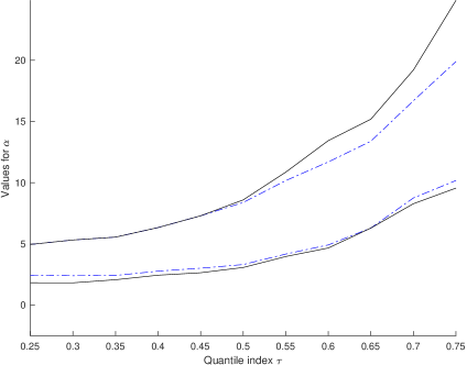
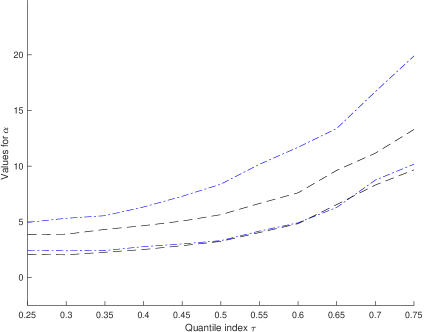
Figure 1: Three point-wise $95\%$ confidence intervals for $\alpha_{0}$. The solid curves represent the proposed inference method, the dash-dotted line ($-.$) curves represent the inference method that assumes $\pi_{0}=\pi_{1}=0$, and the dashed ($--$) curves represent the inference method that assumes $(\pi_{0},\pi_{1})=(0,0.31)$.

The details for the the confidence intervals are as follows. The pre-specified sizes are $(\mathrm{size}_{1},\mathrm{size}_{2})=(1\%,4\%)$, where $\mathrm{size}_{1}$ is used to construct a confidence interval for unknown misclassification probabilities $(\pi_{0},\pi_{1})$ and $\mathrm{size}_{2}$ is used for the critical value $cv$. The confidence interval for $(\pi_{0},\pi_{1})$ is $CI_{1}=\{0\}\times[0,0.31]$ for $(\pi_{0},\pi_{1})$, where $\{0\}$ follows from $E_{n}[D\mid Z=0]=0$ and $[0,0.31]$ comes from the one-tailed $t$-test for $\pi_{1}\leq E[1-D\mid Z=1]$ with size $0.5\%$. The conditional probability of $D$ given $(Y,X,Z)$ is estimated by probit regression of $D$ on all the interactions of $(1,X,Z)$ and the cubic polynomials of $Y$. Using $p_{0}=0$ and grid points $p_{1}=0,0.01,0.02,\ldots,0.31$ for $CI_{1}$, $CI_{\alpha}(\mathrm{size}_{1}+\mathrm{size}_{2})$ is constructed by $\bigcup_{p_{1}=0,0.01,0.02,\ldots,0.31}\left\{\alpha\in\mathcal{A}:T(\alpha;p_{0},p_{1})\leq cv\right\}$.

Figure 1 (left) shows the $95\%$ confidence intervals based on Section 5, with the specification in Eq. (5) and the same list of covariates as Benjamin (2003) and Chernozhukov and Hansen (2004). The figure also shows the $95\%$ confidence intervals that assume $\pi_{0}=\pi_{1}=0$, i.e., no misclassification. The confidence intervals that assume $\pi_{0}=\pi_{1}=0$ are exactly the same as the confidence intervals proposed in Chernozhukov and Hansen (2008, Section 3). All the confidence intervals are point-wise, that is, computed separately for each quantile index $\tau$.

In this empirical exercise, the confidence intervals proposed in this paper are comparable in lengths to those that assume no misclassification. There are several features of this empirical exercise that make the confidence intervals tight (compared to those that assume no misclassification). First, in this empirical exercise, $E_{n}[D\mid Z=z_{0}]=0$ implies $\pi_{0}=0$, so under-identification for $q(\cdot,\tau)$ mainly comes from under-identification for the scalar parameter $\pi_{1}$. It makes the degree of under-identification smaller than when $\pi_{0}$ and $\pi_{1}$ are both under-identified. Second, the confidence intervals that assume $\pi_{0}=\pi_{1}=0$, are large enough to include the confidence interval with another value of $(p_{0},p_{1})$. Figure 1 (right) shows the confidence intervals that assume $(p_{0},p_{1})=(0,0)$ and that with $(p_{0},p_{1})=(0,0.31)$, where the points $(0,0)$ and $(0,0.31)$ are the two endpoints for $CI_{1}$. The confidence intervals that assume $(p_{0},p_{1})=(0,0)$ include those that assume $(p_{0},p_{1})=(0,0.31)$ for almost all the values of $\tau$.

6.2 Monte Carlo simulations

Monte Carlo simulations are based on the following data generating process. The instrumental variable $Z$ takes $z_{0}$ with probability $0.5$ and $z_{1}$ with probability $0.5$. The error term $(\tilde{U},V)$ is a two-dimensional mean-zero normal random vector with variance $1$ and correlation coefficient $0.5$, independent of $Z$. The covariate $X$ is $X=(1,\tilde{X})$, where $\tilde{X}$ is a four-dimensional standard normal random vector with identity covariance matrix, independent of $(Z,\tilde{U},V)$. The latent treatment variable $D^{\ast}$ is determined by

$$D^{\ast}=1\{1\{Z=z_{1}\}+X^{\prime}\beta+V>0\},$$

and the outcome variable $Y$ is determined by

$$Y=\exp(\Phi(\tilde{U})-0.5)D^{\ast}+X^{\prime}\beta+\tilde{U},$$

where $\Phi$ is the standard normal cumulative distribution function and $\beta=(-(2\times 1)^{-1},-(2\times 2)^{-1},\ldots,-(2\times 5)^{-1})^{\prime}$. The binary measurement $D$ is determined by $Pr(D\neq D^{\ast}\mid D^{\ast})=\pi_{D^{\ast}}$, where $(\pi_{0},\pi_{1})=(0,0),(0.1,0),(0,0.1),(0.2,0),(0.1,0.1),(0,0.2),(0.2,0.1),(0.1,0.2)$. The true values for $\alpha_{0}$ is $\exp(\tau-0.5)$.

In this simulation exercise coverage frequencies are computed for two inference methods over $[\alpha_{0}-1,\alpha_{0}+1]$. One is the proposed inference method and the other is the inference method that assumes no misclassification, that is, $\pi_{0}=\pi_{1}=0$. All the results are based on $n=1,000$, $(\mathrm{size}_{1},\mathrm{size}_{2})=(1\%,4\%)$, and 5,000 simulations.

Figure 6.a summarizes the simulation results when there is no misclassification, that is, $(\pi_{0},\pi_{1})=(0,0)$. In this case, both the proposed method and the method that assumes $\pi_{0}=\pi_{1}=0$ have correct size, i.e., the coverage frequency at the true value of $\alpha$ is at least 95%. The proposed inference method is less powerful than that with $\pi_{0}=\pi_{1}=0$, but this is the cost for achieving robustness to misclassification.

Figures 6.b-6.h summarize the simulation results when there is some misclassification. The method that assumes $\pi_{0}=\pi_{1}=0$ does not have correct size as $(\pi_{0},\pi_{1})$ becomes far from $(0,0)$, but the proposed method always has correct size. This is consistent with Theorem 5, which shows that the proposed method has correct size even in the presence of misclassification.

To summarize these simulation results, the proposed inference method covers the true parameter value at least with the pre-specified significance level in finite samples. A practitioner could obtain a narrower confidence interval by assuming no misclassification, but the confidence interval may not cover the true parameter with correct size when there is non-negligible misclassification.

To investigate Monte Carlo simulations, Online Appendix provides a comparison between the proposed inference method and the infeasible method with knowing $(p_{0},p_{1})=(\pi_{0},\pi_{1})$. The details are provided online in supplementary material associated with this article, available at Cambridge Journals Online (journals.cambridge.org/ect).

7 Conclusion

This paper extends the instrumental variable quantile regression model (Chernozhukov and Hansen, 2005, 2013) for a binary regressor, to situations when this binary regressor is potentially misclassified. The first identification result is that under the rank similarity condition and the stochastic monotonicity condition, the reduced-form question effect, $Q_{Y\mid Z=z_{1}}(\tau)-Q_{Y\mid Z=z_{0}}(\tau)$, is biased towards zero compared to the structural quantile treatment effect $q(1,\tau)-q(0,\tau)$. The second identification result characterizes the sharp identified set for $q(d^{\ast},\tau)$ under widely-used assumptions. An inference method for the structural quantile function is provided, and its finite sample performance is demonstrated in simulation studies and an empirical illustration.

Figure 2: *

Figure 6.a: $\pi_{0}=\pi_{1}=0$.

Figure 3: *

Figure 6.b: $\pi_{0}=0.1$ and $\pi_{1}=0$.

Figure 4: *

Figure 6.c: $\pi_{0}=0$ and $\pi_{1}=0.1$.

Figure 5: *

Figure 6.d: $\pi_{0}=0.2$ and $\pi_{1}=0$.

Figure 6: Coverage frequencies. The dash-dot ($-.$) curve represents the proposed inference method, and the dashed ($--$) curve represents the inference method that assumes $\pi_{0}=\pi_{1}=0$.

Figure 7: *

Figure 6.e: $\pi_{0}=\pi_{1}=0.1$.

Figure 8: *

Figure 6.f: $\pi_{0}=0$ and $\pi_{1}=0.2$.

Figure 9: *

Figure 6.g: $\pi_{0}=0.2$ and $\pi_{1}=0.1$.

Figure 10: *

Figure 6.h: $\pi_{0}=0.1$ and $\pi_{1}=0.2$.

Figure 11: *

Figure 6 (continued): Coverage frequencies. The dash-dot ($-.$) curve represents the proposed inference method, and the dashed ($--$) curve represents the inference method that assumes $\pi_{0}=\pi_{1}=0$.

Appendix

Appendix A discusses the identified set when the outcome variable is discrete, and Appendix B provides the proofs for the results in the main text.

Appendix A: Identified set with a discrete outcome variable

This appendix demonstrates how to modify Theorem 2 when the outcome variable is discrete. Assumptions 1-2 are modified into the following two conditions.

Assumption 14.

The mapping $u\mapsto q(d^{\ast},u)$ is weakly increasing and left-continuous for every $u\in[0,1]$.

Assumption 15.

(i) $Pr(U_{0}\leq\tau\mid Z)\geq\tau$ and $Pr(U_{1}\leq\tau\mid Z)\geq\tau$. (ii) $Pr(U_{0}\leq\tau\mid D^{\ast},Z)=Pr(U_{1}\leq\tau\mid D^{\ast},Z)$.

Under the above two assumptions, Theorem 2 can be modified as follows:

Theorem 6.

Assume that all the elements in $\mathcal{Q}\times\mathcal{P}^{\ast}$ satisfy Assumptions 3, 14, and 15. (a) Given a distribution $P$ for the observed variables, if $(y_{0},y_{1})$ belongs to the sharp identified set for $q(\cdot,\tau)$, then

$$P(Y\leq y_{D}\mid Z)-\tau\geq p_{1}(P(Y\leq y_{0}\mid Z)-\tau)+p_{0}(P(Y\leq y_{1}\mid Z)-\tau)$$ (6)

for some $(p_{0},p_{1})$ with $p_{0}+p_{1}<1$ such that $0\leq p_{0}\leq P(D=1\mid Y,Z)\mbox{ a.s.}$ and $0\leq p_{1}\leq P(D=0\mid Y,Z)\mbox{ a.s.}$ (b) The converse is also true if $\mathcal{Q}\times\mathcal{P}^{\ast}$ includes all $(q,P^{\ast})$’s satisfying Assumptions 3, 14, and 15.

Proof.

The proof for (a) is as follows. Define $(p_{0},p_{1})=(\pi_{0},\pi_{1})$. By Assumption 3,

$$\left(\begin{array}[]{ccc}P^{\ast}(D^{\ast}=0\mid Y,Z)\\ P^{\ast}(D^{\ast}=1\mid Y,Z)\end{array}\right)=(1-p_{0}-p_{1})^{-1}\left(\begin{array}[]{ccc}P(D=0\mid Y,Z)-p_{1}\\ P(D=1\mid Y,Z)-p_{0}\\ \end{array}\right).$$ (7)

Using Eq. (7),

$$P(Y\leq y_{D}\mid Z)-p_{1}P(Y\leq y_{0}\mid Z)-p_{0}P(Y\leq y_{1}\mid Z)=(1-p_{0}-p_{1})P(Y\leq y_{D^{\ast}}\mid Z).$$

Since Assumption 14 implies $P(Y\leq y_{D^{\ast}}\mid Z)=P(q(D^{\ast},U)\leq q(D^{\ast},\tau)\mid Z)\geq P(U\leq\tau\mid Z)=P(U_{0}\leq\tau\mid Z)\geq\tau$, it follows that $P(Y\leq y_{D}\mid Z)-p_{1}P(Y\leq y_{0}\mid Z)-p_{0}P(Y\leq y_{1}\mid Z)\geq(1-p_{0}-p_{1})\tau$, and then Eq. (6) holds. Moreover, by Eq. (7), $P^{\ast}(D^{\ast}=d^{\ast}\mid Y,Z)\geq 0$ implies $P(D=0\mid Y,Z)\geq p_{1}$ and $P(D=1\mid Y,Z)\geq p_{0}$.

In the proof for (b), it is necessary to find $(\tilde{q},\tilde{P}^{\ast})\in\mathcal{Q}\times\mathcal{P}^{\ast}$ such that $\tilde{q}(d^{\ast},\tau)=y_{d^{\ast}}$ and that $P$ is the distribution for $(Y,D,Z)$ under $\tilde{P}^{\ast}$. For each $d^{\ast}=0,1$, there is a strictly increasing bijection $t_{d^{\ast}}:[0,1]\rightarrow[0,1]$ such that $t_{d^{\ast}}(\tau)=F_{Y\mid D=d^{\ast}}(y_{d^{\ast}})$. For each $d^{\ast}=0,1$ and every $u\in[0,1]$, define $\tilde{q}(d^{\ast},u)=Q_{Y\mid D=d^{\ast}}(t_{d^{\ast}}(u))$. Define the distribution $\tilde{P}^{\ast}$ for $(D,Z,U_{0},U_{1},D^{\ast})$ by

$$\tilde{P}^{\ast}(D=1-d^{\ast}\mid Z,U_{0},U_{1},D^{\ast}) = p_{D^{\ast}}$$

$$\tilde{P}^{\ast}(Z\leq z,U_{0}\leq u_{0},U_{1}\leq u_{1},D^{\ast}=d^{\ast}) = \tilde{P}^{\ast}(Y\leq q(d^{\ast},\min\{u_{0},u_{1}\}),Z\leq z,D^{\ast}=d^{\ast}),$$

where

$$\left(\begin{array}[]{ccc}\tilde{P}^{\ast}(Y\leq y,Z\leq z,D^{\ast}=0)\\ \tilde{P}^{\ast}(Y\leq y,Z\leq z,D^{\ast}=1)\end{array}\right)=\left(\begin{array}[]{cc}1-p_{0}&p_{1}\\ p_{0}&1-p_{1}\end{array}\right)^{-1}\left(\begin{array}[]{ccc}P(Y\leq y,Z\leq z,D=0)\\ P(Y\leq y,Z\leq z,D=1)\end{array}\right).$$ (8)

By construction, the distribution for $(Y,D,Z)$ under $(\tilde{q},\tilde{P}^{\ast})$ is $P$, and $\tilde{q}(d^{\ast},\tau)=y_{d^{\ast}}$ for each $d^{\ast}=0,1$. To show $(\tilde{q},\tilde{P}^{\ast})\in\mathcal{Q}\times\mathcal{P}^{\ast}$, it suffices to show that Assumptions 14 and 3 hold for $(\tilde{q},\tilde{P}^{\ast})$. The rest of the proof is going to show Assumption 2 (i). By rearranging Eq. (6),

$$\tau \leq \frac{1-p_{1}}{1-p_{0}-p_{1}}P(Y\leq y_{0},D=0\mid Z)-\frac{p_{1}}{1-p_{0}-p_{1}}P(Y\leq y_{0},D=1\mid Z)$$

$$-\frac{p_{0}}{1-p_{0}-p_{1}}P(Y\leq y_{1},D=0\mid Z)+\frac{1-p_{0}}{1-p_{0}-p_{1}}P(Y\leq y_{1},D=1\mid Z)$$

Using Eq. (8), $\tau\leq\tilde{P}^{\ast}(Y\leq y_{0},D^{\ast}=0\mid Z)+\tilde{P}^{\ast}(Y\leq y_{1},D^{\ast}=1\mid Z)$. The definition of $\tilde{q}$ and $\tilde{P}^{\ast}$ implies

$$\tilde{P}^{\ast}(U_{0}\leq\tau\mid Z)=\tilde{P}^{\ast}(Y\leq y_{0},D^{\ast}=0\mid Z)+\tilde{P}^{\ast}(Y\leq y_{1},D^{\ast}=1\mid Z)\geq\tau$$

$$\tilde{P}^{\ast}(U_{1}\leq\tau\mid Z)=\tilde{P}^{\ast}(Y\leq y_{0},D^{\ast}=0\mid Z)+\tilde{P}^{\ast}(Y\leq y_{1},D^{\ast}=1\mid Z)\geq\tau,$$

which is Assumption 2 (i). ∎

Appendix B: Proofs of the results in the main text

Proof of Theorem 1

Lemma 5.

Under Assumptions 1 and 2, $Q_{Y\mid Z}(\tau)$ is a convex combination of $q(1,\tau)$ and $q(0,\tau)$.

Proof.

By the monotonicity of $q(\cdot,d^{\ast})$ and Lemma 1,

$$\tau=P(Y\leq q(D^{\ast},\tau)\mid Z)\geq P(Y\leq\min\{q(1,\tau),q(0,\tau)\}\mid Z)=F_{Y\mid Z}(\min\{q(1,\tau),q(0,\tau)\})$$

$$\tau=P(Y\leq q(D^{\ast},\tau)\mid Z)\leq P(Y\leq\max\{q(1,\tau),q(0,\tau)\}\mid Z)=F_{Y\mid Z}(\max\{q(1,\tau),q(0,\tau)\}).$$

Since $Q_{Y\mid Z}(\cdot)$ is monotonic, it follows that $\min\{q(1,\tau),q(0,\tau)\}\leq Q_{Y\mid Z}(\tau)\leq\max\{q(1,\tau),q(0,\tau)\}$. ∎

By Lemma 5, the statement of theorem holds if $q(1,\tau)=q(0,\tau)$. The rest of the proof is going to focus on $q(1,\tau)>q(0,\tau)$. By Lemma 5, there is some $\kappa\in[-1,1]$ such that $Q_{Y\mid Z=z_{1}}(\tau)-Q_{Y\mid Z=z_{0}}(\tau)=\kappa(q(1,\tau)-q(0,\tau))$. Here it is sufficient to show $Q_{Y\mid Z=z_{1}}(\tau)\geq Q_{Y\mid Z=z_{0}}(\tau)$ for Theorem 1 (a) and $Q_{Y\mid Z=z_{1}}(\tau)>Q_{Y\mid Z=z_{0}}(\tau)$ for Theorem 1 (b). Since $Q_{Y\mid Z}(\tau)$ is a convex combination of $q(1,\tau)$ and $q(0,\tau)$, it follows $q(1,\tau)\geq Q_{Y\mid Z}(\tau)\geq q(0,\tau)$. Since

$$P(Y\leq Q_{Y\mid Z}(\tau),D^{\ast}=0\mid Z)+P(Y\leq Q_{Y\mid Z}(\tau),D^{\ast}=1\mid Z)$$

$$\quad=F_{Y\mid Z}(Q_{Y\mid Z}(\tau))$$

$$\quad=\tau$$

$$\quad=P(q(D^{\ast},U)\leq q(D^{\ast},\tau)\mid Z)$$

$$\quad=P(q(0,U)\leq q(0,\tau),D^{\ast}=0\mid Z)+P(q(1,U)\leq q(1,\tau),D^{\ast}=1\mid Z),$$

it follows that $P(q(0,\tau)<q(0,U)\leq Q_{Y\mid Z}(\tau),D^{\ast}=0\mid Z)=P(Q_{Y\mid Z}(\tau)<q(1,U)\leq q(1,\tau),D^{\ast}=1\mid Z)$. Using the monotonicity of $u\mapsto q(d^{\ast},u)$, $P(\tau<U\leq q^{-1}(Q_{Y\mid Z}(\tau),0),D^{\ast}=0\mid Z)=P(q^{-1}(Q_{Y\mid Z}(\tau),1)<U\leq\tau,D^{\ast}=1\mid Z)$. Using the density function $f_{U_{d^{\ast}},D^{\ast}\mid Z}(y,d^{\ast})$, the above equation can be rewritten as

$$\int_{\tau}^{q^{-1}(Q_{Y\mid Z}(\tau),0)}f_{U_{0},D^{\ast}\mid Z}(u,0)du=\int_{q^{-1}(Q_{Y\mid Z}(\tau),1)}^{\tau}f_{U_{1},D^{\ast}\mid Z}(u,1)du.$$ (9)

The first half of this proof is going to show Theorem 1 (a). Evaluate Eq. (9) at $Z=z_{0}$ and then

$$\int_{\tau}^{q^{-1}(Q_{Y\mid Z=z_{0}}(\tau),0)}f_{U_{0},D^{\ast}\mid Z=z_{0}}(u,0)du=\int_{q^{-1}(Q_{Y\mid Z=z_{0}}(\tau),1)}^{\tau}f_{U_{1},D^{\ast}\mid Z=z_{0}}(u,1)du.$$

Since $f_{U_{0},D^{\ast}\mid Z=z_{1}}(u,0)\leq f_{U_{0},D^{\ast}\mid Z=z_{0}}(u,0)$ and $f_{U_{1},D^{\ast}\mid Z=z_{1}}(u,1)\geq f_{U_{1},D^{\ast}\mid Z=z_{0}}(u,1)$,

$$\int_{\tau}^{q^{-1}(Q_{Y\mid Z=z_{0}}(\tau),0)}f_{U_{0},D^{\ast}\mid Z=z_{1}}(u,0)du\leq\int_{q^{-1}(Q_{Y\mid Z=z_{0}}(\tau),1)}^{\tau}f_{U_{1},D^{\ast}\mid Z=z_{1}}(u,1)du.$$

Subtracting the above equation from Eq. (9) at $Z=z_{1}$, and then

$$\int_{q^{-1}(Q_{Y\mid Z=z_{1}}(\tau),0)}^{q^{-1}(Q_{Y\mid Z=z_{0}}(\tau),0)}f_{U_{0},D^{\ast}\mid Z=z_{1}}(u,0)du\leq\int_{q^{-1}(Q_{Y\mid Z=z_{0}}(\tau),1)}^{q^{-1}(Q_{Y\mid Z=z_{1}}(\tau),1)}f_{U_{1},D^{\ast}\mid Z=z_{1}}(u,1)du.$$

Using $Y=q(D^{\ast},U)$,

$$\int_{Q_{Y\mid Z=z_{1}}(\tau)}^{Q_{Y\mid Z=z_{0}}(\tau)}f_{Y,D^{\ast}\mid Z=z_{1}}(y,0)dy\leq\int_{Q_{Y\mid Z=z_{0}}(\tau)}^{Q_{Y\mid Z=z_{1}}(\tau)}f_{Y,D^{\ast}\mid Z=z_{1}}(y,1)dy,$$

and then $\int_{Q_{Y\mid Z=z_{0}}(\tau)}^{Q_{Y\mid Z=z_{1}}(\tau)}f_{Y,D^{\ast}\mid Z=z_{1}}(u)du\geq 0$, which implies $\tau-F_{Y,D^{\ast}\mid Z=z_{1}}(Q_{Y\mid Z=z_{0}}(\tau))\geq 0$.

The second half of the proof is going to show Theorem 1 (b). To the contrary, suppose $Q_{Y\mid Z=z_{0}}(\tau)\leq Q_{Y\mid Z=z_{1}}(\tau)$. By Theorem 1 (a), $Q_{Y\mid Z=z_{0}}(\tau)=Q_{Y\mid Z=z_{1}}(\tau)$. Using $\Delta f_{U_{d^{\ast}},D^{\ast}\mid Z}(u,d^{\ast})=f_{U_{d^{\ast}},D^{\ast}\mid Z=z_{1}}(u,d^{\ast})-f_{U_{d^{\ast}},D^{\ast}\mid Z=z_{0}}(u,d^{\ast})$, Eq. (9) implies

$$\int_{\tau}^{q^{-1}(Q_{Y\mid Z=z_{0}}(\tau),0)}\Delta f_{U_{0},D^{\ast}\mid Z}(u,0)du=\int_{q^{-1}(Q_{Y\mid Z=z_{0}}(\tau),1)}^{\tau}\Delta f_{U_{1},D^{\ast}\mid Z}(u,1)du.$$

Since $f_{U_{0},D^{\ast}\mid Z=z_{1}}(u,0)\leq f_{U_{0},D^{\ast}\mid Z=z_{0}}(u,0)$ and $f_{U_{1},D^{\ast}\mid Z=z_{1}}(u,1)\geq f_{U_{1},D^{\ast}\mid Z=z_{0}}(u,1)$,

$$\int_{\tau}^{q^{-1}(Q_{Y\mid Z=z_{0}}(\tau),0)}|\Delta f_{U_{0},D^{\ast}\mid Z}(u,0)|du=-\int_{q^{-1}(Q_{Y\mid Z=z_{0}}(\tau),1)}^{\tau}|\Delta f_{U_{1},D^{\ast}\mid Z}(u,1)|du.$$

Since $f_{U_{0},D^{\ast}\mid Z=z_{1}}(u,0)<f_{U_{0},D^{\ast}\mid Z=z_{0}}(u,0)$ and $f_{U_{1},D^{\ast}\mid Z=z_{1}}(u,1)>f_{U_{1},D^{\ast}\mid Z=z_{0}}(u,1)$ in a neighborhood of $\tau$, the above equation implies $q^{-1}(Q_{Y\mid Z=z_{0}}(\tau),0)=\tau=q^{-1}(Q_{Y\mid Z=z_{0}}(\tau),1)$, which contradicts $q(1,\tau)>q(0,\tau)$.

Proof of Theorem 2

The proof for (a) is as follows. By Assumption 3,

$$\left(\begin{array}[]{ccc}P^{\ast}(D^{\ast}=0\mid Y,Z)\\ P^{\ast}(D^{\ast}=1\mid Y,Z)\end{array}\right) = (1-\pi_{0}-\pi_{1})^{-1}\left(\begin{array}[]{ccc}P(D=0\mid Y,Z)-\pi_{1}\\ P(D=1\mid Y,Z)-\pi_{0}\\ \end{array}\right).$$

Eq. (1) in Lemma 1 becomes Eq. (4). Moreover, $P^{\ast}(D^{\ast}=d^{\ast}\mid Y,Z)\geq 0$ implies $P(D=0\mid Y,Z)\geq\pi_{1}$ and $P(D=1\mid Y,Z)\geq\pi_{0}$.

In the proof for (b), it is necessary to find $(\tilde{q},\tilde{P}^{\ast})\in\mathcal{Q}\times\mathcal{P}^{\ast}$ such that $\tilde{q}(d^{\ast},\tau)=y_{d^{\ast}}$ and that $P$ is the distribution for $(Y,D,Z)$ under $\tilde{P}^{\ast}$. For each $d^{\ast}=0,1$, there is a strictly increasing bijection $t_{d^{\ast}}:[0,1]\rightarrow[0,1]$ such that $t_{d^{\ast}}(\tau)=F_{Y\mid D=d^{\ast}}(y_{d^{\ast}})$. For each $d^{\ast}=0,1$ and every $u\in[0,1]$, define $\tilde{q}(d^{\ast},u)=Q_{Y\mid D=d^{\ast}}(t_{d^{\ast}}(u))$. Define the distribution $\tilde{P}^{\ast}$ for $(D,Z,U_{0},U_{1},D^{\ast})$ by

$$\tilde{P}^{\ast}(D\neq D^{\ast}\mid Z,U_{0},U_{1},D^{\ast}) = p_{D^{\ast}}$$

$$\tilde{P}^{\ast}(Z\leq z,U_{0}\leq u_{0},U_{1}\leq u_{1},D^{\ast}=d^{\ast}) = \tilde{P}^{\ast}(Y\leq q(d^{\ast},\min\{u_{0},u_{1}\}),Z\leq z,D^{\ast}=d^{\ast}),$$

where

$$\left(\begin{array}[]{ccc}\tilde{P}^{\ast}(Y\leq y,Z\leq z,D^{\ast}=0)\\ \tilde{P}^{\ast}(Y\leq y,Z\leq z,D^{\ast}=1)\end{array}\right)=\left(\begin{array}[]{cc}1-p_{0}&p_{1}\\ p_{0}&1-p_{1}\end{array}\right)^{-1}\left(\begin{array}[]{ccc}P(Y\leq y,Z\leq z,D=0)\\ P(Y\leq y,Z\leq z,D=1)\end{array}\right).$$ (11)

By construction, the distribution for $(Y,D,Z)$ under $(\tilde{q},\tilde{P}^{\ast})$ is $P$, and $\tilde{q}(d^{\ast},\tau)=y_{d^{\ast}}$ for each $d^{\ast}=0,1$. To show $(\tilde{q},\tilde{P}^{\ast})\in\mathcal{Q}\times\mathcal{P}^{\ast}$, it suffices to show that Assumptions 1, 2, and 3 hold for $(\tilde{q},\tilde{P}^{\ast})$. The rest of the proof is going to show Assumption 2 (i). By rearranging Eq. (4),

$$\tau = \frac{1-p_{1}}{1-p_{0}-p_{1}}P(Y\leq y_{0},D=0\mid Z)-\frac{p_{1}}{1-p_{0}-p_{1}}P(Y\leq y_{0},D=1\mid Z)$$

$$-\frac{p_{0}}{1-p_{0}-p_{1}}P(Y\leq y_{1},D=0\mid Z)+\frac{1-p_{0}}{1-p_{0}-p_{1}}P(Y\leq y_{1},D=1\mid Z)$$

Using Eq. (11), $\tau=\tilde{P}^{\ast}(Y\leq y_{0},D^{\ast}=0\mid Z)+\tilde{P}^{\ast}(Y\leq y_{1},D^{\ast}=1\mid Z)$. The definition of $\tilde{q}$ and $\tilde{P}^{\ast}$ implies

$$\tilde{P}^{\ast}(U_{0}\leq\tau\mid Z)=\tilde{P}^{\ast}(Y\leq y_{0},D^{\ast}=0\mid Z)+\tilde{P}^{\ast}(Y\leq y_{1},D^{\ast}=1\mid Z)=\tau$$

$$\tilde{P}^{\ast}(U_{1}\leq\tau\mid Z)=\tilde{P}^{\ast}(Y\leq y_{0},D^{\ast}=0\mid Z)+\tilde{P}^{\ast}(Y\leq y_{1},D^{\ast}=1\mid Z)=\tau.$$

Proof of Corollary 1

Use $(p_{0},p_{1})=(0,0)$. Then $(y_{0},y_{1})$ satisfies the conditions in Theorem 2.

Proof of Corollary 2

In this proof, assume $Q_{Y\mid Z=z_{0}}(\tau)\leq Q_{Y\mid Z=z_{1}}(\tau)$ without loss of generality. The “only if” part of this corollary is shown as follows. By Theorem 2, Eq. (4) holds for some $(p_{0},p_{1})$ with $0\leq p_{0}\leq P(D=1\mid Y,Z)$ a.s. and $0\leq p_{1}\leq P(D=0\mid Y,Z)$ a.s. Using $(y_{0},y_{1})=(Q_{Y\mid Z=z_{0}}(\tau),Q_{Y\mid Z=z_{1}}(\tau))$, Eq. (4) becomes

$$P(y_{0}<Y\leq y_{1},D=1\mid Z=z_{0})=p_{0}P(y_{0}<Y\leq y_{1}\mid Z=z_{0})$$

$$-P(y_{0}<Y\leq y_{1},D=0\mid Z=z_{1})=-p_{1}P(y_{0}<Y\leq y_{1}\mid Z=z_{1}).$$

Since $p_{0}\leq P(D=1\mid Y,Z)$ a.s. and $p_{1}\leq P(D=0\mid Y,Z)$ a.s., it follows that $P(D=1\mid y_{0}<Y\leq y_{1},Z=z_{0})\leq P(D=1\mid Y,Z)$ a.s. and $P(D=0\mid y_{0}<Y\leq y_{1},Z=z_{1})\leq P(D=0\mid Y,Z)$ a.s.

The “if” part of this corollary is shown by choosing $p_{0}=P(D=1\mid y_{0}<Y\leq y_{1},Z=z_{0})$ and $p_{1}=P(D=0\mid y_{0}<Y\leq y_{1},Z=z_{1})$.

Proof of Theorem 3

Assume $\bar{d}^{\ast}=0$ for simplicity. Note that $q(d^{\ast},u)=Q_{Y\mid D^{\ast}=d^{\ast},Z}(u)$ from Condition (iii). Take sufficiently small $\varepsilon>0$ and define

$$\left(\tilde{q}(0,u),\tilde{q}(1,u)\right) = \left(q\left(0,u+\frac{\varepsilon}{1-\pi_{0}-\pi_{1}}(u-P^{\ast}(Y\leq q(1,u)\mid D^{\ast}=0))\right),q(1,u)\right)$$

$$({p}_{0},{p}_{1}) = (\pi_{0}-\varepsilon,\pi_{1}).$$

Condition (iv) guarantees $p_{0}\geq 0$. Consider $U_{0}=U_{1}$ and define $\tilde{P}^{\ast}$ by

$$\tilde{P}^{\ast}(\tilde{q}(0,U_{0})\leq y,D^{\ast}=0,Z\leq z) = \frac{1-\pi_{0}-\pi_{1}}{1-\pi_{0}-\pi_{1}+\varepsilon}P^{\ast}(Y\leq y,D^{\ast}=0,Z\leq z)$$

$$\tilde{P}^{\ast}(\tilde{q}(1,U_{1})\leq y,D^{\ast}=1,Z\leq z) = P^{\ast}(Y\leq y,D^{\ast}=1,Z\leq z)$$

$$\quad+\frac{\varepsilon}{1-\pi_{0}-\pi_{1}+\varepsilon}P^{\ast}(Y\leq y,D^{\ast}=0,Z\leq z)$$

$$\tilde{P}^{\ast}(D=0\mid Z,U_{1},D^{\ast}=1) = \pi_{1}$$

$$\tilde{P}^{\ast}(D=1\mid Z,U_{0},D^{\ast}=0) = \pi_{0}-\varepsilon.$$

By Condition (ii), $u\neq P^{\ast}(Y\leq q(1,u)\mid D^{\ast}=0)$ and $\tilde{q}(0,\tau)\neq q\left(0,u\right)$ as long as $\varepsilon$ is positive. To establish the statement of this theorem, the rest of the proof is going to show that $(\tilde{q},\tilde{P}^{\ast})\in\mathcal{Q}\times\mathcal{P}^{\ast}$ and that $(\tilde{q},\tilde{P}^{\ast})$ is observationally equivalent to $(q,P^{\ast})$.

First, $(\tilde{q},\tilde{P}^{\ast})\in\mathcal{Q}\times\mathcal{P}^{\ast}$. The Lipschitz continuity in Condition (i) guarantees that $u\mapsto t(u)$ is a strictly increasing bijection of $[0,1]$ into $[0,1]$ for sufficiently small $\varepsilon$, where $t(u)=u+\frac{\varepsilon}{1-\pi_{0}-\pi_{1}}(u-P^{\ast}(Y\leq q(1,u)\mid D^{\ast}=0)$. Therefore, Condition (v) implies $\tilde{q}\in\mathcal{Q}$ for sufficiently small $\varepsilon$. To show $\tilde{P}^{\ast}\in\mathcal{P}^{\ast}$, it suffices to show Assumption 2 (i) because Assumption 2 (ii) holds for $U=U_{0}=U_{1}$. By the definition of $\tilde{q}$ and independence between $Z$ and $Y$ given $D^{\ast}$,

$$P^{\ast}(Y\leq\tilde{q}(0,\tau),D^{\ast}=0\mid Z) = P^{\ast}(D^{\ast}=0\mid Z)P^{\ast}(Y\leq\tilde{q}(0,\tau)\mid D^{\ast}=0)$$

$$= P^{\ast}(D^{\ast}=0\mid Z)\left(\tau+\frac{\varepsilon}{1-\pi_{0}-\pi_{1}}(\tau-P^{\ast}(Y\leq q(1,\tau)\mid D^{\ast}=0))\right)$$

$$= P^{\ast}(D^{\ast}=0\mid Z)\left(\tau+\frac{\varepsilon}{1-\pi_{0}-\pi_{1}}(\tau-P^{\ast}(Y\leq q(1,\tau)\mid D^{\ast}=0,Z))\right),$$

where the second equality uses $q(0,u)=Q_{Y\mid D^{\ast}=0}(u)$. By the definition of $\tilde{P}^{\ast}$ and $\tilde{q}$,

$$\tilde{P}^{\ast}(U\leq\tau\mid Z) = \frac{1-\pi_{0}-\pi_{1}}{1-\pi_{0}-\pi_{1}+\varepsilon}P^{\ast}(D^{\ast}=0\mid Z)\left(\tau+\frac{\varepsilon}{1-\pi_{0}-\pi_{1}}(\tau-P^{\ast}(Y\leq q(1,\tau)\mid D^{\ast}=0,Z))\right)$$

$$\quad+P^{\ast}(Y\leq q(1,\tau),D^{\ast}=1\mid Z)+\frac{\varepsilon}{1-\pi_{0}-\pi_{1}+\varepsilon}P^{\ast}(Y\leq q(1,\tau),D^{\ast}=0\mid Z)$$

$$= \tau P^{\ast}(D^{\ast}=0\mid Z)+P^{\ast}(Y\leq q(1,\tau),D^{\ast}=1\mid Z)$$

$$= \tau,$$

where the last equality uses $q(1,u)=Q_{Y\mid D^{\ast}=1,Z}(u)$.

Second, $(\tilde{q},\tilde{P}^{\ast})$ is observationally equivalent to $(q,P^{\ast})$. By the definition of $\tilde{P}^{\ast}$,

$$\tilde{P}^{\ast}(Y\leq y,D^{\ast}=1,Z\leq z) = \tilde{P}^{\ast}(\tilde{q}(1,U)\leq y,D^{\ast}=1,Z\leq z)$$

$$= P^{\ast}(Y\leq y,D^{\ast}=1,Z\leq z)+\frac{\varepsilon}{1-\pi_{0}-\pi_{1}+\varepsilon}P^{\ast}(Y\leq y,D^{\ast}=0,Z\leq z)$$

$$\tilde{P}^{\ast}(Y\leq y,D^{\ast}=0,Z\leq z) = \tilde{P}^{\ast}(\tilde{q}(0,U)\leq y,D^{\ast}=0,Z\leq z)$$

$$= \frac{1-\pi_{0}-\pi_{1}}{1-\pi_{0}-\pi_{1}+\varepsilon}P^{\ast}(Y\leq y,D^{\ast}=0,Z\leq z).$$

Therefore,

$$\tilde{P}(Y\leq y,D=0,Z\leq z) = \tilde{P}^{\ast}(D=0\mid Z,U_{0},U_{1},D^{\ast}=0)\tilde{P}(Y\leq y,D^{\ast}=0,Z\leq z)$$

$$\quad+\tilde{P}^{\ast}(D=0\mid Z,U_{0},U_{1},D^{\ast}=1)\tilde{P}(Y\leq y,D^{\ast}=1,Z\leq z)$$

$$= (1-\pi_{0}+\varepsilon)\frac{1-\pi_{0}-\pi_{1}}{1-\pi_{0}-\pi_{1}+\varepsilon}P^{\ast}(Y\leq y,D^{\ast}=0,Z\leq z)$$

$$+\pi_{1}P^{\ast}(Y\leq y,D^{\ast}=1,Z\leq z)$$

$$+\pi_{1}\frac{\varepsilon}{1-\pi_{0}-\pi_{1}+\varepsilon}P^{\ast}(Y\leq y,D^{\ast}=0,Z\leq z)$$

$$= (1-\pi_{0})P^{\ast}(Y\leq y,D^{\ast}=0,Z\leq z)$$

$$+\pi_{1}P^{\ast}(Y\leq y,D^{\ast}=1,Z\leq z)$$

$$= P^{\ast}(Y\leq y,D=0,Z\leq z)$$

and it can be similarly shown that $\tilde{P}(Y\leq y,D=1,Z\leq z)=P^{\ast}(Y\leq y,D=1,Z\leq z)$.

Proof of Lemma 2

Under Assumption 4 (i),

$$f_{(D,V)\mid Z}(d,v) = \left(\begin{array}[]{cc}f_{D\mid D^{\ast}=0,Z}(d)&f_{D\mid D^{\ast}=1,Z}(d)\end{array}\right)\left(\begin{array}[]{cc}f_{D^{\ast}\mid Z}(0)&0\\ 0&f_{D^{\ast}\mid Z}(1)\end{array}\right)\left(\begin{array}[]{cc}f_{V\mid D^{\ast}=0}(v)\\ f_{V\mid D^{\ast}=1}(v)\end{array}\right).$$

Under Assumption 3,

$$\left(\begin{array}[]{cc}f_{(D,V)\mid Z}(0,v_{0})&f_{(D,V)\mid Z}(0,v_{1})\\ f_{(D,V)\mid Z}(1,v_{0})&f_{(D,V)\mid Z}(1,v_{1})\\ \end{array}\right)$$

$$\quad\quad\quad=\left(\begin{array}[]{cc}1-\pi_{0}&\pi_{1}\\ \pi_{0}&1-\pi_{1}\end{array}\right)\left(\begin{array}[]{cc}f_{D^{\ast}\mid Z}(0)&0\\ 0&f_{D^{\ast}\mid Z}(1)\end{array}\right)\left(\begin{array}[]{cc}f_{V\mid D^{\ast}=0}(v_{0})&f_{V\mid D^{\ast}=0}(v_{1})\\ f_{V\mid D^{\ast}=1}(v_{0})&f_{V\mid D^{\ast}=1}(v_{1})\\ \end{array}\right).$$

Under Assumption 4 (ii) and (iii), the above matrix for $Z=z_{1}$ is invertible, so

$$\begin{pmatrix}f_{(D,V)\mid Z=z_{0}}(0,v_{0})&f_{(D,V)\mid Z=z_{0}}(0,v_{1})\\ f_{(D,V)\mid Z=z_{0}}(1,v_{0})&f_{(D,V)\mid Z=z_{0}}(1,v_{1})\\ \end{pmatrix}\begin{pmatrix}f_{(D,V)\mid Z=z_{1}}(0,v_{0})&f_{(D,V)\mid Z=z_{1}}(0,v_{1})\\ f_{(D,V)\mid Z=z_{1}}(1,v_{0})&f_{(D,V)\mid Z=z_{1}}(1,v_{1})\\ \end{pmatrix}^{-1}$$

$$=\begin{pmatrix}1-\pi_{0}&\pi_{1}\\ \pi_{0}&1-\pi_{1}\end{pmatrix}\begin{pmatrix}f_{D^{\ast}\mid Z=z_{0}}(0)/f_{D^{\ast}\mid Z=z_{1}}(0)&0\\ 0&f_{D^{\ast}\mid Z=z_{0}}(1)/f_{D^{\ast}\mid Z=z_{1}}(1)\end{pmatrix}\begin{pmatrix}1-\pi_{0}&\pi_{1}\\ \pi_{0}&1-\pi_{1}\end{pmatrix}^{-1}$$

Under Assumption 4 (iv), the eigenvalue decomposition of the above matrix is uniquely determined, so $(\pi_{0},\pi_{1})$ is identified. Since $f_{(Y,D)\mid Z}(y,d)=\sum_{d^{\ast}=0,1}f_{D\mid Y=y,D^{\ast}=d^{\ast},Z}(d)f_{(Y,D^{\ast})\mid Z}(y,d^{\ast})$, Assumption 3 implies

$$f_{(Y,D)\mid Z}(y,0) = \pi_{0}f_{(Y,D^{\ast})\mid Z}(y,1)+(1-\pi_{0})f_{(Y,D^{\ast})\mid Z}(y,0)$$

$$f_{(Y,D)\mid Z}(y,1) = (1-\pi_{1})f_{(Y,D^{\ast})\mid Z}(y,1)+\pi_{1}f_{(Y,D^{\ast})\mid Z}(y,0),$$

so that $f_{(Y,D^{\ast})\mid Z}$ is point identified.

Proof of Lemma 3

It follows from Theorem 2 of Chernozhukov and Hansen (2013).

Proof of Theorem 4

It follows from Lemmas 2 and 3.

Proof of Lemma 4

Note that

$$(1-\pi_{0}-\pi_{1})E[\rho_{\tau}(Y-\alpha_{0}D^{\ast}-W^{\prime}\theta)]$$

$$\quad=(1-\pi_{0}-\pi_{1})E[\rho_{\tau}(Y-W^{\prime}\theta)(1-D^{\ast})]+(1-\pi_{0}-\pi_{1})E[\rho_{\tau}(Y-\alpha_{0}-W^{\prime}\theta)D^{\ast}]$$

$$\quad=(1-\pi_{1})E[\rho_{\tau}(Y-W^{\prime}\theta)(1-D)]-\pi_{1}E[\rho_{\tau}(Y-W^{\prime}\theta)D]$$

$$\quad-\pi_{0}E[\rho_{\tau}(Y-\alpha_{0}-W^{\prime}\theta)(1-D)]+(1-\pi_{0})E[\rho_{\tau}(Y-\alpha_{0}-W^{\prime}\theta)D]$$

$$\quad=E[\rho_{\tau}(Y-W^{\prime}\theta)(1-\pi_{1}-D)]]+E[\rho_{\tau}(Y-\alpha_{0}-W^{\prime}\theta)(D-\pi_{0})]$$

$$\quad=E[\rho_{\tau}(Y-W^{\prime}\theta)(1-\pi_{1}-E[D\mid Y,X,Z])]]+E[\rho_{\tau}(Y-\alpha_{0}-W^{\prime}\theta)(E[D\mid Y,X,Z]-\pi_{0})],$$

because

$$\left(\begin{array}[]{cc}1-\pi_{0}&\pi_{1}\\ \pi_{0}&1-\pi_{1}\end{array}\right)^{-1}=\frac{1}{1-\pi_{0}-\pi_{1}}\left(\begin{array}[]{cc}1-\pi_{1}&-\pi_{1}\\ -\pi_{0}&1-\pi_{0}\end{array}\right).$$

Since $Pr(Y-\alpha_{0}D^{\ast}\leq X^{\prime}\beta_{0}+0\cdot Z\mid X,Z)=Pr(q(D^{\ast},X,U)\leq q(D^{\ast},X,\tau)\mid X,Z)=\tau$, Chernozhukov and Hansen (2008, p.383) derives $0\in\operatorname*{arg\,min}_{\gamma}\left(\min_{\beta}E[\rho_{\tau}(Y-\alpha_{0}D^{\ast}-W^{\prime}\theta)]\right)$. Therefore,

$$0\in\operatorname*{arg\,min}_{\gamma}\left(\min_{\beta}E[\rho_{\tau}(Y-W^{\prime}\theta)(1-\pi_{1}-\nu_{0}(Y,X,Z))]+E[\rho_{\tau}(Y-\alpha_{0}-W^{\prime}\theta)(\nu_{0}(Y,X,Z)-\pi_{0})]\right).$$

Note that $\nu_{0}(Y,X,Z)-\pi_{0}=(\nu_{0}(Y,X,Z)-\pi_{0})_{+}$ and $1-\pi_{1}-\nu_{0}(Y,X,Z)=(1-\pi_{1}-\nu_{0}(Y,X,Z))_{+}$, because

$$E[D\mid Y,X,Z]=\pi_{0}+(1-\pi_{0}-\pi_{1})E[D^{\ast}\mid Y,X,Z]\geq\pi_{0}$$

$$1-E[D\mid Y,X,Z]=\pi_{1}+(1-\pi_{0}-\pi_{1})E[1-D^{\ast}\mid Y,X,Z]\geq\pi_{1}.$$

Proof of Theorem 5

By Lemma 10 and 14 below, $P(T(\alpha_{0};\pi_{0},\pi_{1})\leq cv)\rightarrow 1-\mathrm{size}_{2}$ as $n\rightarrow\infty$. Then the theorem follows from

$$P(\alpha_{0}\in CI_{\alpha}(\mathrm{size}_{1}+\mathrm{size}_{2})) \geq P(\{\alpha_{0}\in CI_{\alpha}(\mathrm{size}_{1}+\mathrm{size}_{2})\}\cap\{(\pi_{0},\pi_{1})\in CI_{1}\})$$

$$\geq P(\{T(\alpha_{0};\pi_{0},\pi_{1})\leq cv\}\cap\{(\pi_{0},\pi_{1})\in CI_{1}\})$$

$$\geq P(T(\alpha_{0};\pi_{0},\pi_{1})\leq cv)-P((\pi_{0},\pi_{1})\notin CI_{1})$$

and then $\liminf_{n\rightarrow\infty}P(\alpha_{0}\in CI_{\alpha}(\mathrm{size}_{1}+\mathrm{size}_{2}))\geq 1-(\mathrm{size}_{1}+\mathrm{size}_{2})$.

The following proof assumes $1-\pi_{1}-\hat{\nu}(Y,X,Z)\geq 0$ and $\hat{\nu}(Y,X,Z)-\pi_{0}\geq 0$ without loss of generality, because $E[D^{\ast}\mid Y,X,Z]$ is bounded away from zero and one, and then

$$1-\pi_{1}-\hat{\nu}(Y,X,Z)=(1-\pi_{0}-\pi_{1})E[1-D^{\ast}\mid Y,X,Z]-(\hat{\nu}(Y,X,Z)-{\nu}(Y,X,Z))>0$$

$$\hat{\nu}(Y,X,Z)-\pi_{0}=(1-\pi_{0}-\pi_{1})E[D^{\ast}\mid Y,X,Z]+(\hat{\nu}(Y,X,Z)-{\nu}(Y,X,Z))>0$$

with probability approaching one.

Lemma 6.

$\sup_{\theta\in\Theta}|\bar{Q}_{n}(\theta)-\bar{Q}_{0}(\theta)|=o_{p}(1)$, where $\bar{Q}_{n}(\theta)=Q_{n}(\theta;\alpha_{0},\pi_{0},\pi_{1})$ and $\bar{Q}_{0}(\theta)=Q_{0}(\theta;\alpha_{0},\pi_{0},\pi_{1})$.

Proof.

The proof of this lemma is to check the conditions in Newey and McFadden (1994, Lemma 2.9). Since $\Theta$ is compact and $\bar{Q}_{0}$ is continuous, it suffices to show $\bar{Q}_{n}(\theta)=\bar{Q}_{0}(\theta)+o_{p}(1)$ for every $\theta\in\Theta$ and $|\bar{Q}_{n}(\tilde{\theta})-\bar{Q}_{n}(\theta)|\leq 2E_{n}\left[\|W\|\right]\cdot\|\tilde{\theta}-\theta\|$ for every $\tilde{\theta},\theta\in\Theta$. This proof uses

$$\bar{Q}_{n}^{\ast}(\theta)=E_{n}[\rho_{\tau}(Y-W^{\prime}\theta)(1-\pi_{1}-\nu_{0}(Y,X,Z))_{+}]+E_{n}[\rho_{\tau}(Y-\alpha_{0}-W^{\prime}\theta)(\nu_{0}(Y,X,Z)-\pi_{0})_{+}].$$

The pointwise convergence of $\bar{Q}_{n}(\theta)$ to $\bar{Q}_{0}(\theta)$ is shown by demonstrating $\bar{Q}_{n}(\theta)-\bar{Q}_{n}^{\ast}(\theta)=o_{p}(1)$ and $\bar{Q}_{n}^{\ast}(\theta)-\bar{Q}_{0}(\theta)=o_{p}(1)$. Since

$$|\bar{Q}_{n}(\theta)-\bar{Q}_{n}^{\ast}(\theta)| \leq E_{n}[\rho_{\tau}(Y-W^{\prime}\theta)|\hat{\nu}(Y,X,Z)-\nu_{0}(Y,X,Z)|]$$

$$\qquad+E_{n}[\rho_{\tau}(Y-\alpha_{0}-W^{\prime}\theta)|\hat{\nu}(Y,X,Z)-\nu_{0}(Y,X,Z)|]$$

$$\leq \sup_{(y,x,z)}|\hat{\nu}(y,x,z)-\nu_{0}(y,x,z)|\left(E_{n}[|\rho_{\tau}(Y-W^{\prime}\theta)|+|\rho_{\tau}(Y-\alpha_{0}-W^{\prime}\theta)|]\right),$$

Assumption 10 (ii) implies $\bar{Q}_{n}(\theta)-\bar{Q}_{n}^{\ast}(\theta)=o_{p}(1)$. Moreover, $\bar{Q}_{n}^{\ast}(\theta)-\bar{Q}_{0}(\theta)=\bar{Q}_{n}^{\ast}(\theta)-E[\bar{Q}_{n}^{\ast}(\theta)]=o_{p}(1)$ is shown by checking the second moment of $\bar{Q}_{n}^{\ast}(\theta)$: $E[\bar{Q}_{n}^{\ast}(\theta)^{2}]=O(1/n)$ follows from

$$E\left[\left(\rho_{\tau}(Y-W^{\prime}\theta)(1-\pi_{1}-D)+\rho_{\tau}(Y-\alpha_{0}-W^{\prime}\theta)(D-\pi_{0})\right)^{2}\right]^{1/2}$$

$$\quad\leq E\left[\left(Y-W^{\prime}\theta\right)^{2}\right]^{1/2}+E\left[\left(Y-\alpha_{0}-W^{\prime}\theta\right)^{2}\right]^{1/2}$$

$$\quad\leq 2E\left[Y^{2}\right]^{1/2}+\alpha_{0}+2E\left[\|W\|^{2}\right]^{1/2}\left\|\theta\right\|$$

$$\quad<\infty.$$

The in-probability Lipschitz condition is shown as follows. Since $|\rho_{\tau}(Y-W^{\prime}\theta)-\rho_{\tau}(Y-W^{\prime}\tilde{\theta})|\leq|W^{\prime}(\tilde{\theta}-\theta)|\leq\|W\|\cdot\left\|\tilde{\theta}-\theta\right\|$ and $|\rho_{\tau}(Y-\alpha_{0}-W^{\prime}\theta)-\rho_{\tau}(Y-\alpha_{0}-W^{\prime}\tilde{\theta})|\leq\|W\|\cdot\left\|\tilde{\theta}-\theta\right\|$, it follows that $|\bar{Q}_{n}(\tilde{\theta})-\bar{Q}_{n}(\theta)|\leq E_{n}\left[\|W\|\cdot\left\|\tilde{\theta}-\theta\right\|\right]+E_{n}\left[\|W\|\cdot\left\|\tilde{\theta}-\theta\right\|\right]\leq 2E_{n}\left[\|W\|\right]\cdot\left\|\tilde{\theta}-\theta\right\|$. ∎

Lemma 7.

$\hat{\theta}_{0}-\theta_{0}=o_{p}(1)$, where $\hat{\theta}_{0}=\hat{\theta}(\alpha_{0};\pi_{0},\pi_{1})$.

Proof.

The proof of this lemma is to check the conditions in Newey and McFadden (1994, Theorem 2.1) to establish the consistency. Since $\Theta$ is compact, $\bar{Q}_{0}$ is continuous, and Lemma 6 establishes the uniform convergence of $\bar{Q}_{n}(\theta)$, it suffices to show that $\bar{Q}_{0}$ is uniquely minimized at $\theta_{0}$. As in the proof of Lemma 4,

$$\bar{Q}_{0}(\theta) = E\left[\rho_{\tau}(Y-W^{\prime}\theta)(1-\pi_{1}-D)+\rho_{\tau}(Y-\alpha_{0}-W^{\prime}\theta)(D-\pi_{0})\right]$$

$$= (1-\pi_{0}-\pi_{1})E\left[\rho_{\tau}(Y-\alpha_{0}D^{\ast}-W^{\prime}\theta)\right]$$

Since

$$\frac{\partial}{\partial\theta}\bar{Q}_{0}(\theta)=(1-\pi_{0}-\pi_{1})\frac{\partial}{\partial\theta}E\left[\rho_{\tau}(Y-\alpha_{0}D^{\ast}-W^{\prime}\theta)\right]=(1-\pi_{0}-\pi_{1})E\left[(F_{Y-\alpha_{0}D^{\ast}\mid X,Z}(W^{\prime}\theta)-\tau)W\right]$$

$$\frac{\partial^{2}}{\partial\theta\partial\theta^{\prime}}\bar{Q}_{0}(\theta)=(1-\pi_{0}-\pi_{1})E\left[f_{Y-\alpha_{0}D^{\ast}\mid X,Z}(W^{\prime}\theta)WW^{\prime}\right],$$

it follows that $\frac{\partial}{\partial\theta}\bar{Q}_{0}(\theta_{0})=0$ and $\frac{\partial^{2}}{\partial\theta\partial\theta^{\prime}}\bar{Q}_{0}(\theta)$ is positive semidefinite everywhere and positive definite at $\theta_{0}$. Therefore, $\bar{Q}_{0}$ is uniquely minimized at $\theta_{0}$. ∎

Lemma 8.

$E_{n}\left[\xi_{0}(\hat{\nu})W\right]=E_{n}[s_{0}]+o_{p}(n^{-1/2})$, where $s_{0}=\xi_{0}(\nu_{0})W+E\left[W\Xi_{0}(\delta_{0})\right]\psi_{\delta}$.

Proof.

By Assumption 10 (iii)-(iv), $E_{n}\left[\xi_{0}(\hat{\nu})W\right]=E_{n}\left[\xi_{0}(\nu_{0})W\right]+E\left[W\Xi_{0}(\delta_{0})\right]E_{n}[\psi_{\delta}]+o_{p}(n^{-1/2})$. ∎

Lemma 9.

Define

$$\lambda_{0}(\bm{\tau}) = f_{Y\mid D,Z,X}(W^{\prime}\theta_{0}-n^{-1/2}W^{\prime}\bm{\tau})(1-\pi_{1}-D)+f_{Y\mid D,Z,X}(\alpha_{0}+W^{\prime}\theta_{0}-n^{-1/2}W^{\prime}\bm{\tau})(D-\pi_{0})$$

$$g(\bm{\tau},\nu) = (\rho_{\tau}(Y-W^{\prime}\theta_{0}-n^{-1/2}W^{\prime}\bm{\tau})-\rho_{\tau}(Y-W^{\prime}\theta_{0}))(1-\pi_{1}-\nu(Y,X,Z))_{+}$$

$$+(\rho_{\tau}(Y-\alpha_{0}-W^{\prime}\theta_{0}-n^{-1/2}W^{\prime}\bm{\tau})-\rho_{\tau}(Y-\alpha_{0}-W^{\prime}\theta_{0}))(\nu(Y,X,Z)-\pi_{0})_{+}$$

$$r_{n}(\bm{\tau}) = nE_{n}[g(\bm{\tau},\hat{\nu})]-\frac{1}{2}\bm{\tau}^{\prime}E[\lambda_{0}(0)WW^{\prime}]\bm{\tau}+\sqrt{n}\bm{\tau}^{\prime}E_{n}\left[\xi_{0}(\hat{\nu})W\right].$$

Then $\sup_{\bm{\tau}}|r_{n}(\bm{\tau})|=o_{p}(1)$.

Proof.

If $r_{n}(\bm{\tau})=o_{p}(1)$ pointwise in $\bm{\tau}$, it is possible to the convexity lemma in Pollard (1991) to $\bm{\tau}\mapsto nE_{n}[g(\bm{\tau},\hat{\nu})]+\sqrt{n}\bm{\tau}^{\prime}E_{n}\left[\xi_{0}(\hat{\nu})W\right]$, and then $\sup_{\bm{\tau}}|r_{n}(\bm{\tau})|=o_{p}(1)$. Therefore, it suffices to show that $r_{n}(\bm{\tau})=o_{p}(1)$ pointwise in $\bm{\tau}$. Note that

$$E[\lambda_{0}(0)WW^{\prime}] = E\left[f_{Y\mid D,Z,X}(W^{\prime}\theta_{0})(1-\pi_{1}-\nu_{0}(Y,X,Z))_{+}WW^{\prime}\right]$$

$$+E\left[f_{Y\mid D,Z,X}(\alpha_{0}+W^{\prime}\theta_{0})(\nu_{0}(Y,X,Z)-\pi_{0})_{+}WW^{\prime}\right],$$

where the equality uses the law of iterated expectation, $(1-\pi_{1}-\nu_{0}(Y,X,Z))_{+}=1-\pi_{1}-\nu_{0}(Y,X,Z)$ and $(\nu_{0}(Y,X,Z)-\pi_{0})_{+}=\nu_{0}(Y,X,Z)-\pi_{0}$. Therefore, $\left.\frac{\partial}{\partial\bm{\tau}}E[ng(\bm{\tau},\nu_{0})]\right|_{\bm{\tau}=0}=-n^{1/2}E\left[\xi_{0}(\nu_{0})W\right]\ =0$ and $\frac{\partial^{2}}{\partial\bm{\tau}\partial\bm{\tau}^{\prime}}E[ng(\tau,\nu_{0})]=E[\lambda_{0}(\bm{\tau})WW^{\prime}]=E[\lambda_{0}(0)WW^{\prime}]+o(1)$, so that

$$E[ng(\bm{\tau},\nu_{0})]=\frac{1}{2}\bm{\tau}^{\prime}E[\lambda_{0}(0)WW^{\prime}]\bm{\tau}+o(1).$$

Therefore,

$$r_{n}(\bm{\tau}) = nE_{n}[g(\bm{\tau},\hat{\nu})]-nE[g(\bm{\tau},\nu_{0})]+\sqrt{n}\bm{\tau}^{\prime}E_{n}\left[\xi_{0}(\hat{\nu})W\right]+o(1).$$

$$= E_{n}\left[ng(\bm{\tau},\hat{\nu})+\sqrt{n}\bm{\tau}^{\prime}\xi_{0}(\hat{\nu})W\right]-E_{n}\left[ng(\bm{\tau},\nu_{0})+\sqrt{n}\bm{\tau}^{\prime}\xi_{0}(\nu_{0})W\right]$$

$$+E_{n}\left[ng(\bm{\tau},\nu_{0})+\sqrt{n}\bm{\tau}^{\prime}\xi_{0}(\nu_{0})W\right]-E[ng(\bm{\tau},\nu_{0})]+o(1)$$

$$= E_{n}\left[n(g(\bm{\tau},\hat{\nu})-g(\bm{\tau},\nu_{0}))+\sqrt{n}\bm{\tau}^{\prime}(\xi_{0}(\hat{\nu})-\xi_{0}(\nu_{0}))W\right]$$

$$+(E_{n}-E)[ng(\bm{\tau},\nu_{0})+\sqrt{n}\bm{\tau}^{\prime}\xi_{0}(\nu_{0})W]+o(1),$$

where the last equality follows from $E[\bm{\tau}^{\prime}\xi_{0}(\nu_{0})W]=0$.

First, $E_{n}\left[n(g(\bm{\tau},\hat{\nu})-g(\bm{\tau},\nu_{0}))+\sqrt{n}\bm{\tau}^{\prime}(\xi_{0}(\hat{\nu})-\xi_{0}(\nu_{0}))W\right]$ converges to zero in $L^{1}$. By the definitions of $g(\bm{\tau},{\nu})$ and $\xi_{0}(\nu)$,

$$n(g(\bm{\tau},\hat{\nu})-g(\bm{\tau},\nu_{0}))+\sqrt{n}\bm{\tau}^{\prime}(\xi_{0}(\hat{\nu})-\xi_{0}(\nu_{0}))W$$

$$= n\times\mathrm{term}_{1}\times((1-\pi_{1}-\hat{\nu}(Y,X,Z))_{+}-(1-\pi_{1}-\nu_{0}(Y,X,Z)))$$

$$+n\times\mathrm{term}_{2}\times((\hat{\nu}(Y,X,Z)-\pi_{0})_{+}-(\nu_{0}(Y,X,Z)-\pi_{0})),$$

where $\mathrm{term}_{1}=\rho_{\tau}(Y-W^{\prime}(\theta_{0}-n^{-1/2}\bm{\tau}))-\rho_{\tau}(Y-W^{\prime}\theta_{0})+(\tau-1\{Y-W^{\prime}\theta_{0}\leq 0\})n^{-1/2}W^{\prime}\bm{\tau}$ and $\mathrm{term}_{2}=\rho_{\tau}(Y-\alpha_{0}-W^{\prime}(\theta_{0}-n^{-1/2}\bm{\tau}))-\rho_{\tau}(Y-\alpha_{0}-W^{\prime}\theta_{0})+(\tau-1\{Y-\alpha_{0}-W^{\prime}\theta_{0}\leq 0\})n^{-1/2}W^{\prime}\bm{\tau}$. By the definition of $\rho_{\tau}$, the two terms, $\mathrm{term}_{1}$ and $\mathrm{term}_{2}$, can be bounded as follows:

$$\left|\mathrm{term}_{1}\right| \leq 1\{|Y-W^{\prime}\theta_{0}|\leq|n^{-1/2}W^{\prime}\bm{\tau}|\}\left(|Y-W^{\prime}\theta_{0}|+|n^{-1/2}W^{\prime}\bm{\tau}|\right)$$ (15)

$$\leq 1\{|Y-W^{\prime}\theta_{0}|\leq|n^{-1/2}W^{\prime}\bm{\tau}|\}\times 2|n^{-1/2}W^{\prime}\bm{\tau}|$$

$$\left|\mathrm{term}_{2}\right| \leq 1\{|Y-\alpha_{0}-W^{\prime}\theta_{0}|\leq|n^{-1/2}W^{\prime}\bm{\tau}|\}\left(|Y-\alpha_{0}-W^{\prime}\theta_{0}|+|n^{-1/2}W^{\prime}\bm{\tau}|\right)$$ (16)

$$\leq 1\{|Y-\alpha_{0}-W^{\prime}\theta_{0}|\leq|n^{-1/2}W^{\prime}\bm{\tau}|\}\times 2|n^{-1/2}W^{\prime}\bm{\tau}|.$$

As long as $1-\pi_{1}-\hat{\nu}(Y,X,Z)\geq 0$ and $\hat{\nu}(Y,X,Z)-\pi_{0}\geq 0$,

$$|(1-\pi_{1}-\hat{\nu}(Y,X,Z))_{+}-(1-\pi_{1}-\nu_{0}(Y,X,Z))| = |(1-\pi_{1}-\hat{\nu}(Y,X,Z))-(1-\pi_{1}-\nu_{0}(Y,X,Z))|$$ (17)

$$\leq \sup_{(y,x,z)}|\hat{\nu}(y,x,z)-\nu_{0}(y,x,z)|$$

$$|(\hat{\nu}(Y,X,Z)-\pi_{0})_{+}-(\nu_{0}(Y,X,Z)-\pi_{0})| = |(\hat{\nu}(Y,X,Z)-\pi_{0})-(\nu_{0}(Y,X,Z)-\pi_{0})|$$ (18)

$$\leq \sup_{(y,x,z)}|\hat{\nu}(y,x,z)-\nu_{0}(y,x,z)|.$$

Now it is possible to bound $E\left[\left\|E_{n}\left[n(g(\bm{\tau},\hat{\nu})-g(\bm{\tau},\nu_{0}))+\sqrt{n}\bm{\tau}^{\prime}(\xi_{0}(\hat{\nu})-\xi_{0}(\nu_{0}))W\right]\right\|\right]$ as follows:

$$E\left[\left\|E_{n}\left[n(g(\bm{\tau},\hat{\nu})-g(\bm{\tau},\nu_{0}))+\sqrt{n}\bm{\tau}^{\prime}(\xi_{0}(\hat{\nu})-\xi_{0}(\nu_{0}))W\right]\right\|\right]$$

$$\leq E\left[\left|n(g(\bm{\tau},\hat{\nu})-g(\bm{\tau},\nu_{0}))+\sqrt{n}\bm{\tau}^{\prime}(\xi_{0}(\hat{\nu})-\xi_{0}(\nu_{0}))\right|\left\|W\right\|\right]$$

$$\leq 2nE[1\{|Y-W^{\prime}\theta_{0}|\leq|n^{-1/2}W^{\prime}\bm{\tau}|\}|n^{-1/2}W^{\prime}\bm{\tau}|\left\|W\right\|]\sup_{(y,x,z)}|\hat{\nu}(y,x,z)-\nu_{0}(y,x,z)|$$

$$+2nE[1\{|Y-\alpha_{0}-W^{\prime}\theta_{0}|\leq|n^{-1/2}W^{\prime}\bm{\tau}|\}|n^{-1/2}W^{\prime}\bm{\tau}|\left\|W\right\|]\sup_{(y,x,z)}|\hat{\nu}(y,x,z)-\nu_{0}(y,x,z)|$$

Since $|f_{Y\mid X,Z}|\leq C$, it follows that

$$E[1\{|Y-W^{\prime}\theta_{0}|\leq|n^{-1/2}W^{\prime}\bm{\tau}|\}|n^{-1/2}W^{\prime}\bm{\tau}|\left\|W\right\|]\leq 2Cn^{-1}E[|W^{\prime}\bm{\tau}|^{2}\left\|W\right\|]$$

$$E[1\{|Y-\alpha_{0}-W^{\prime}\theta_{0}|\leq|n^{-1/2}W^{\prime}\bm{\tau}|\}|n^{-1/2}W^{\prime}\bm{\tau}|\left\|W\right\|]\leq 2Cn^{-1}E[|W^{\prime}\bm{\tau}|^{2}\left\|W\right\|],$$

so that

$$E\left[\left|n(g(\bm{\tau},\hat{\nu})-g(\bm{\tau},\nu_{0}))+\sqrt{n}\bm{\tau}^{\prime}(\xi_{0}(\hat{\nu})-\xi_{0}(\nu_{0}))\right|\left\|W\right\|\right]$$

$$\qquad\leq 8CE[|W^{\prime}\bm{\tau}|^{2}\left\|W\right\|]\sup_{(y,x,z)}|\hat{\nu}(y,x,z)-\nu_{0}(y,x,z)|$$

$$\qquad=o(1).$$

Next, $(E_{n}-E)[ng(\bm{\tau},\nu_{0})+\sqrt{n}\bm{\tau}^{\prime}\xi_{0}(\nu_{0})W]$ converges to zero in $L^{2}$. Using the bounds in Eq. (15)-(18),

$$E[(ng(\bm{\tau},\nu_{0})+\sqrt{n}\bm{\tau}^{\prime}\xi_{0}(\nu_{0})W)^{2}]^{1/2}$$

$$\leq nE[\left|\mathrm{term}_{1}\right|^{2}\times((1-\pi_{1}-\hat{\nu}(Y,X,Z))_{+}-(1-\pi_{1}-\nu_{0}(Y,X,Z)))^{2}]^{1/2}$$

$$+nE[\left|\mathrm{term}_{2}\right|^{2}\times((\hat{\nu}(Y,X,Z)-\pi_{0})_{+}-(\nu_{0}(Y,X,Z)-\pi_{0}))^{2}]^{1/2}$$

$$\leq 4nE[1\{|Y-W^{\prime}\theta_{0}|\leq|n^{-1/2}W^{\prime}\bm{\tau}|\}\times|n^{-1/2}W^{\prime}\bm{\tau}|^{2}]^{1/2}\sup_{(y,x,z)}|\hat{\nu}(y,x,z)-\nu_{0}(y,x,z)|.$$

$$+4nE[1\{|Y-\alpha_{0}-W^{\prime}\theta_{0}|\leq|n^{-1/2}W^{\prime}\bm{\tau}|\}\times|n^{-1/2}W^{\prime}\bm{\tau}|^{2}]^{1/2}\sup_{(y,x,z)}|\hat{\nu}(y,x,z)-\nu_{0}(y,x,z)|$$

$$\leq 8n^{1/2}E[|W^{\prime}\bm{\tau}|^{2}]^{1/2}\sup_{(y,x,z)}|\hat{\nu}(y,x,z)-\nu_{0}(y,x,z)|$$

$$= o(n^{1/2}),$$

and then $E[((E_{n}-E)[ng(\bm{\tau},\nu_{0})+\sqrt{n}\bm{\tau}^{\prime}\xi_{0}(\nu_{0})W])^{2}]=n^{-1}E[(ng(\bm{\tau},\nu_{0})+\sqrt{n}\bm{\tau}^{\prime}\xi_{0}(\nu_{0})W)^{2}]=o(1)$. ∎

Lemma 10.

$\sqrt{n}(\hat{\theta}_{0}-\theta_{0})=\sqrt{n}E[\lambda_{0}(0)WW^{\prime}]^{-1}E_{n}[s_{0}]+o_{p}(1)$ and therefore $\sqrt{n}(\hat{\theta}_{0}-\theta_{0})\rightarrow_{d}N\left(0,\Omega_{0}\right)$ as $n\rightarrow\infty$, where $\Omega_{0}=E[\lambda_{0}(0)WW^{\prime}]^{-1}E[s_{0}s_{0}^{\prime}]E[\lambda_{0}(0)WW^{\prime}]^{-1}.$

Proof.

Define $\eta_{n}=\sqrt{n}E[\lambda_{0}(0)WW^{\prime}]^{-1}E_{n}[s_{0}]$. It suffices to show $\sqrt{n}(\hat{\theta}_{0}-\theta_{0})=\eta_{n}+o_{p}(1)$. By Lemma 8, $\eta_{n}=\sqrt{n}E[\lambda_{0}(0)WW^{\prime}]^{-1}E_{n}\left[\xi_{0}(\hat{\nu})W\right]+o_{p}(1).$ Using the definition of $r_{n}(\cdot)$,

$$-\frac{1}{2}\eta_{n}^{\prime}E[\lambda_{0}(0)WW^{\prime}]\eta_{n}+r_{n}(\eta_{n}) = nE_{n}[g(\eta_{n},\hat{\nu})]$$

$$\geq nE_{n}[g(\sqrt{n}(\hat{\theta}_{0}-\theta_{0}),\hat{\nu})]$$

$$= \frac{1}{2}(\sqrt{n}(\hat{\theta}_{0}-\theta_{0})-\eta_{n})^{\prime}E[\lambda_{0}(0)WW^{\prime}](\sqrt{n}(\hat{\theta}_{0}-\theta_{0})-\eta_{n})$$

$$-\frac{1}{2}\eta_{n}^{\prime}E[\lambda_{0}(0)WW^{\prime}]\eta_{n}+r_{n}(\sqrt{n}(\hat{\theta}_{0}-\theta_{0}))$$

$$\geq \frac{1}{2}\|\sqrt{n}(\hat{\theta}_{0}-\theta_{0})-\eta_{n}\|^{2}\mathrm{eig}_{\min}\left(E[\lambda_{0}(0)WW^{\prime}]\right)$$

$$-\frac{1}{2}\eta_{n}^{\prime}E[\lambda_{0}(0)WW^{\prime}]\eta_{n}+r_{n}(\sqrt{n}(\hat{\theta}_{0}-\theta_{0})),$$

where the first inequality uses $\sqrt{n}(\hat{\theta}_{0}-\theta_{0})=\operatorname*{arg\,min}_{\bm{\tau}}E_{n}[g(\bm{\tau},\hat{\nu})]$ and $\mathrm{eig}_{\min}\left(E[\lambda_{0}(0)WW^{\prime}]\right)$ is the minimum eigenvalue of $E[\lambda_{0}(0)WW^{\prime}]$. Therefore, $r_{n}(\eta_{n})-r_{n}(\sqrt{n}(\hat{\theta}_{0}-\theta_{0}))\geq\frac{1}{2}\|\sqrt{n}(\hat{\theta}_{0}-\theta_{0})-\eta_{n}\|^{2}\mathrm{eig}_{\min}\left(E[\lambda_{0}(0)WW^{\prime}]\right)$, so that Lemma 9 implies $\sqrt{n}(\hat{\theta}_{0}-\theta_{0})-\eta_{n}=o_{p}(1)$. ∎

Lemma 11.

$Pr(|Y-W^{\prime}\theta_{0}|\leq\|(\hat{\theta}_{0}-\theta_{0})\|\|W\|\})=o(1)$ and $Pr(|Y-\alpha_{0}-W^{\prime}\theta_{0}|\leq\|(\hat{\theta}_{0}-\theta_{0})\|\|W\|\})=o(1)$.

Proof.

By Lemma 10 and Assumption 12 (iii), the first part of this lemma follows from $Pr(|Y-W^{\prime}\theta_{0}|\leq\|(\hat{\theta}_{0}-\theta_{0})\|\|W\|\})\leq Pr(\|(\hat{\theta}_{0}-\theta_{0})\|\leq n^{-1/2}\log(n))+Pr(|Y-W^{\prime}\theta_{0}|\leq n^{-1/2}\log(n)\|W\|\})=o(1)$. The second part can be shown similarly. ∎

Lemma 12.

$E_{n}[\hat{s}(\alpha_{0};\pi_{0},\pi_{1})\hat{s}(\alpha_{0};\pi_{0},\pi_{1})^{\prime}]=E[s_{0}s_{0}^{\prime}]+o_{p}(1)$.

Proof.

The weak law of large numbers implies $E_{n}[s_{0}s_{0}^{\prime}]=E[s_{0}s_{0}^{\prime}]+o_{p}(1)$, and then it suffices to show $E_{n}[\hat{s}(\alpha_{0};\pi_{0},\pi_{1})\hat{s}(\alpha_{0};\pi_{0},\pi_{1})^{\prime}-s_{0}s_{0}^{\prime}]=o_{p}(1)$. Since

$$E_{n}[(\hat{s}(\alpha_{0};\pi_{0},\pi_{1})-s_{0})(\hat{s}(\alpha_{0};\pi_{0},\pi_{1})-s_{0})^{\prime}]$$

$$= E_{n}[(\widehat{\xi}(\alpha_{0};\pi_{0},\pi_{1})-\xi_{0}(\nu_{0}))WW^{\prime}(\widehat{\xi}(\alpha_{0};\pi_{0},\pi_{1})-\xi_{0}(\nu_{0}))^{\prime}]$$

$$+E_{n}[(\widehat{\xi}(\alpha_{0};\pi_{0},\pi_{1})-\xi_{0}(\nu_{0}))W\widehat{\psi_{\delta}}^{\prime}]E_{n}\left[W(\widehat{\Xi}(\alpha_{0};\pi_{0},\pi_{1})-\Xi_{0}(\delta_{0}))\right]^{\prime}$$

$$+E_{n}[(\widehat{\xi}(\alpha_{0};\pi_{0},\pi_{1})-\xi_{0}(\nu_{0}))W\widehat{\psi_{\delta}}^{\prime}](E_{n}-E)\left[W\Xi_{0}(\delta_{0})\right]^{\prime}$$

$$+E_{n}[(\widehat{\xi}(\alpha_{0};\pi_{0},\pi_{1})-\xi_{0}(\nu_{0}))W(\widehat{\psi_{\delta}}-\psi_{\delta})^{\prime}]E\left[W\Xi_{0}(\delta_{0})\right]^{\prime}$$

$$+E_{n}\left[W(\widehat{\Xi}(\alpha_{0};\pi_{0},\pi_{1})-\Xi_{0}(\delta_{0}))\right]E_{n}[\widehat{\psi_{\delta}}W^{\prime}(\widehat{\xi}(\alpha_{0};\pi_{0},\pi_{1})-\xi_{0}(\nu_{0}))^{\prime}]$$

$$+E_{n}\left[W(\widehat{\Xi}(\alpha_{0};\pi_{0},\pi_{1})-\Xi_{0}(\delta_{0}))\right]E_{n}[\widehat{\psi_{\delta}}\widehat{\psi_{\delta}}^{\prime}]E_{n}\left[W(\widehat{\Xi}(\alpha_{0};\pi_{0},\pi_{1})-\Xi_{0}(\delta_{0}))\right]^{\prime}$$

$$+E_{n}\left[W(\widehat{\Xi}(\alpha_{0};\pi_{0},\pi_{1})-\Xi_{0}(\delta_{0}))\right]E_{n}[\widehat{\psi_{\delta}}\widehat{\psi_{\delta}}^{\prime}](E_{n}-E)\left[W\Xi_{0}(\delta_{0})\right]^{\prime}$$

$$+E_{n}\left[W(\widehat{\Xi}(\alpha_{0};\pi_{0},\pi_{1})-\Xi_{0}(\delta_{0}))\right]E_{n}[\widehat{\psi_{\delta}}(\widehat{\psi_{\delta}}-\psi_{\delta})^{\prime}]E\left[W\Xi_{0}(\delta_{0})\right]^{\prime}$$

$$+(E_{n}-E)\left[W\Xi_{0}(\delta_{0})\right]E_{n}[\widehat{\psi_{\delta}}W^{\prime}(\widehat{\xi}(\alpha_{0};\pi_{0},\pi_{1})-\xi_{0}(\nu_{0}))^{\prime}]$$

$$+(E_{n}-E)\left[W\Xi_{0}(\delta_{0})\right]E_{n}[\widehat{\psi_{\delta}}\widehat{\psi_{\delta}}^{\prime}]E_{n}\left[W(\widehat{\Xi}(\alpha_{0};\pi_{0},\pi_{1})-\Xi_{0}(\delta_{0}))\right]^{\prime}$$

$$+(E_{n}-E)\left[W\Xi_{0}(\delta_{0})\right]E_{n}[\widehat{\psi_{\delta}}\widehat{\psi_{\delta}}^{\prime}](E_{n}-E)\left[W\Xi_{0}(\delta_{0})\right]^{\prime}$$

$$+(E_{n}-E)\left[W\Xi_{0}(\delta_{0})\right]E_{n}[\widehat{\psi_{\delta}}(\widehat{\psi_{\delta}}-\psi_{\delta})^{\prime}]E\left[W\Xi_{0}(\delta_{0})\right]^{\prime}$$

$$+E\left[W\Xi_{0}(\delta_{0})\right]E_{n}[(\widehat{\psi_{\delta}}-\psi_{\delta})W^{\prime}(\widehat{\xi}(\alpha_{0};\pi_{0},\pi_{1})-\xi_{0}(\nu_{0}))^{\prime}]$$

$$+E\left[W\Xi_{0}(\delta_{0})\right]E_{n}[(\widehat{\psi_{\delta}}-\psi_{\delta})\widehat{\psi_{\delta}}^{\prime}]E_{n}\left[W(\widehat{\Xi}(\alpha_{0};\pi_{0},\pi_{1})-\Xi_{0}(\delta_{0}))\right]^{\prime}$$

$$+E\left[W\Xi_{0}(\delta_{0})\right]E_{n}[(\widehat{\psi_{\delta}}-\psi_{\delta})\widehat{\psi_{\delta}}^{\prime}](E_{n}-E)\left[W\Xi_{0}(\delta_{0})\right]^{\prime}$$

$$+E\left[W\Xi_{0}(\delta_{0})\right]E_{n}[(\widehat{\psi_{\delta}}-\psi_{\delta})(\widehat{\psi_{\delta}}-\psi_{\delta})^{\prime}]E\left[W\Xi_{0}(\delta_{0})\right]^{\prime}$$

and

$$E_{n}[(\hat{s}(\alpha_{0};\pi_{0},\pi_{1})-s_{0})s_{0}^{\prime}]$$

$$\quad=E_{n}[(\widehat{\xi}(\alpha_{0};\pi_{0},\pi_{1})-\xi_{0}(\nu_{0}))WW^{\prime}\xi_{0}(\nu_{0})^{\prime}]+E_{n}[(\widehat{\xi}(\alpha_{0};\pi_{0},\pi_{1})-\xi_{0}(\nu_{0}))W\psi_{\delta}^{\prime}]E\left[W\Xi_{0}(\delta_{0})\right]^{\prime}$$

$$\qquad+E_{n}\left[W(\widehat{\Xi}(\alpha_{0};\pi_{0},\pi_{1})-\Xi_{0}(\delta_{0}))\right]E_{n}[\widehat{\psi_{\delta}}W^{\prime}\xi_{0}(\nu_{0})^{\prime}]$$

$$\qquad+E_{n}\left[W(\widehat{\Xi}(\alpha_{0};\pi_{0},\pi_{1})-\Xi_{0}(\delta_{0}))\right]E_{n}[\widehat{\psi_{\delta}}\psi_{\delta}^{\prime}]E\left[W\Xi_{0}(\delta_{0})\right]^{\prime}$$

$$\qquad+(E_{n}-E)\left[W\Xi_{0}(\delta_{0})\right]E_{n}[\widehat{\psi_{\delta}}W^{\prime}\xi_{0}(\nu_{0})^{\prime}]+(E_{n}-E)\left[W\Xi_{0}(\delta_{0})\right]E_{n}[\widehat{\psi_{\delta}}\psi_{\delta}^{\prime}]E\left[W\Xi_{0}(\delta_{0})\right]^{\prime}$$

$$\qquad+E\left[W\Xi_{0}(\delta_{0})\right]E_{n}[(\widehat{\psi_{\delta}}-\psi_{\delta})W^{\prime}\xi_{0}(\nu_{0})^{\prime}]+E\left[W\Xi_{0}(\delta_{0})\right]E_{n}[(\widehat{\psi_{\delta}}-\psi_{\delta})\psi_{\delta}^{\prime}]E\left[W\Xi_{0}(\delta_{0})\right]^{\prime},$$

it suffices to show that $(E_{n}-E)\left[W\Xi_{0}(\delta_{0})\right]=o_{p}(1)$, that $E_{n}[\widehat{\psi_{\delta}}W^{\prime}\xi_{0}(\nu_{0})^{\prime}]$, $E_{n}[\widehat{\psi_{\delta}}\psi_{\delta}^{\prime}]$, $E_{n}[\widehat{\psi_{\delta}}W^{\prime}\xi_{0}(\nu_{0})^{\prime}]$, and $E_{n}[\widehat{\psi_{\delta}}\psi_{\delta}^{\prime}]$ are $O_{p}(1)$, and that the sample averages of the following variables are $o_{p}(1)$: (1) $(\widehat{\xi}(\alpha_{0};\pi_{0},\pi_{1})-\xi_{0}(\nu_{0}))W\psi_{\delta}^{\prime}$, (2) $(\widehat{\xi}(\alpha_{0};\pi_{0},\pi_{1})-\xi_{0}(\nu_{0}))WW^{\prime}\xi_{0}(\nu_{0})^{\prime}$, (3) $(\widehat{\xi}(\alpha_{0};\pi_{0},\pi_{1})-\xi_{0}(\nu_{0}))WW^{\prime}(\widehat{\xi}(\alpha_{0};\pi_{0},\pi_{1})-\xi_{0}(\nu_{0}))^{\prime}$, (4) $(\widehat{\xi}(\alpha_{0};\pi_{0},\pi_{1})-\xi_{0}(\nu_{0}))W\widehat{\psi_{\delta}}^{\prime}$, (5) $(\widehat{\xi}(\alpha_{0};\pi_{0},\pi_{1})-\xi_{0}(\nu_{0}))W(\widehat{\psi_{\delta}}-\psi_{\delta})^{\prime}$, (6) $W(\widehat{\Xi}(\alpha_{0};\pi_{0},\pi_{1})-\Xi_{0}(\delta_{0}))$, (7) $\widehat{\psi_{\delta}}W^{\prime}(\widehat{\xi}(\alpha_{0};\pi_{0},\pi_{1})-\xi_{0}(\nu_{0}))^{\prime}$, (8) $\widehat{\psi_{\delta}}(\widehat{\psi_{\delta}}-\psi_{\delta})^{\prime}$, (9) $(\widehat{\psi_{\delta}}-\psi_{\delta})W^{\prime}\xi_{0}(\nu_{0})^{\prime}$, (10) $(\widehat{\psi_{\delta}}-\psi_{\delta})W^{\prime}(\widehat{\xi}(\alpha_{0};\pi_{0},\pi_{1})-\xi_{0}(\nu_{0}))^{\prime}$, and (11) $(\widehat{\psi_{\delta}}-\psi_{\delta})(\widehat{\psi_{\delta}}-\psi_{\delta})^{\prime}$. The convergence $(E_{n}-E)\left[W\Xi_{0}(\delta_{0})\right]=o_{p}(1)$ comes from the weak law of large numbers, and the other parts come from a combination of Assumption 10 (iv)-(vii) and the following equalities:

$$E[\|\xi_{0}(\nu_{0})W\|^{2}]<\infty$$ (19)

$$E[\|(\widehat{\xi}(\alpha_{0};\pi_{0},\pi_{1})-\xi_{0}(\nu_{0}))W\|^{2}]=o(1)$$ (20)

$$E\left[W(\widehat{\Xi}(\alpha_{0};\pi_{0},\pi_{1})-\Xi_{0}(\delta_{0}))\right]=o_{p}(1).$$ (21)

Note that Eq. (19) follows from $|\xi_{0}(\nu_{0})|\leq 2$ and $E[\|W\|^{2}]<\infty$.

First, Eq. (20) is shown as follows. Since

$$|\widehat{\xi}(\alpha_{0};\pi_{0},\pi_{1})-\xi_{0}(\nu_{0})| \leq |(1\{Y-W^{\prime}\theta_{0}\leq 0\}-1\{Y-W^{\prime}\hat{\theta}_{0}\leq 0\})|\times|1-\pi_{1}-\hat{\nu}(Y,X,Z)|$$

$$+|\tau-1\{Y-W^{\prime}\theta_{0}\leq 0\}|\times|\nu_{0}(Y,X,Z)-\hat{\nu}(Y,X,Z)|$$

$$+|1\{Y-\alpha_{0}-W^{\prime}\theta_{0}\leq 0\}-1\{Y-\alpha_{0}-W^{\prime}\hat{\theta}_{0}\leq 0\}|\times|\hat{\nu}(Y,X,Z)-\pi_{0}|$$

$$+|\tau-1\{Y-\alpha_{0}-W^{\prime}\theta_{0}\leq 0\}|\times|\hat{\nu}(Y,X,Z)-\nu_{0}(Y,X,Z)|$$

$$\leq 1\{|Y-W^{\prime}\theta_{0}|\leq\|(\hat{\theta}_{0}-\theta_{0})\|\|W\|\}$$

$$+1\{|Y-\alpha_{0}-W^{\prime}\theta_{0}|\leq\|(\hat{\theta}_{0}-\theta_{0})\|\|W\|\}$$

$$+2|\hat{\nu}(Y,X,Z)-\nu_{0}(Y,X,Z)|,$$

it follows that

$$E[\|(\widehat{\xi}(\alpha_{0};\pi_{0},\pi_{1})-\xi_{0}(\nu_{0}))W\|^{2}]^{1/2} \leq Pr(|Y-W^{\prime}\theta_{0}|\leq\|(\hat{\theta}_{0}-\theta_{0})\|\|W\|\})^{1/4}E[\|\|W\|^{4}]^{1/4}$$

$$+Pr(|Y-\alpha_{0}-W^{\prime}\theta_{0}|\leq\|(\hat{\theta}_{0}-\theta_{0})\|\|W\|)^{1/4}E[\|\|W\|^{4}]^{1/4}$$

$$+2E[|\hat{\nu}(Y,X,Z)-\nu_{0}(Y,X,Z)|^{4}]^{1/4}E[\|\|W\|^{4}]^{1/4}.$$

By Assumption 10 (ii) and Lemma 11, Eq. (20) holds.

Next, Eq. (21) is shown as follows. Since

$$\widehat{\Xi}(\alpha_{0};\pi_{0},\pi_{1})-\Xi_{0}(\delta_{0}) = 1\{Y-W^{\prime}\hat{\theta}_{0}\leq 0\}\left(\widehat{\frac{\partial}{\delta^{\prime}}\nu_{\delta}}(Y,X,Z)-{\frac{\partial}{\delta^{\prime}}\nu_{\delta}}(Y,X,Z)\right)$$

$$+\left(1\{Y-W^{\prime}\hat{\theta}_{0}\leq 0\}-1\{Y-W^{\prime}\theta_{0}\leq 0\}\right)\frac{\partial}{\delta^{\prime}}\nu_{\delta}(Y,X,Z)$$

$$-1\{Y-\alpha-W^{\prime}\hat{\theta}_{0}\leq 0\}\left(\widehat{\frac{\partial}{\delta^{\prime}}\nu_{\delta}}(Y,X,Z)-{\frac{\partial}{\delta^{\prime}}\nu_{\delta}}(Y,X,Z)\right)$$

$$-\left(1\{Y-\alpha-W^{\prime}\hat{\theta}_{0}\leq 0\}-1\{Y-\alpha-W^{\prime}\theta_{0}\leq 0\}\right){\frac{\partial}{\delta^{\prime}}\nu_{\delta}}(Y,X,Z),$$

it follows that

$$E\left[\left\|W(\widehat{\Xi}(\alpha_{0};\pi_{0},\pi_{1})-\Xi_{0}(\delta_{0}))\right\|\right]$$

$$\leq 2E\left[\left\|W\left(\widehat{\frac{\partial}{\delta^{\prime}}\nu_{\delta}}(Y,X,Z)-{\frac{\partial}{\delta^{\prime}}\nu_{\delta}}(Y,X,Z)\right)\right\|\right]$$

$$\qquad+Pr(|Y-W^{\prime}\theta_{0}|\leq\|(\hat{\theta}_{0}-\theta_{0})\|\|W\|)^{1/2}E\left[\left\|W\frac{\partial}{\delta^{\prime}}\nu_{\delta}(Y,X,Z)\right\|^{2}\right]^{1/2}$$

$$\qquad+Pr(|Y-\alpha_{0}-W^{\prime}\theta_{0}|\leq\|(\hat{\theta}_{0}-\theta_{0})\|\|W\|)^{1/2}E\left[\left\|W\frac{\partial}{\delta^{\prime}}\nu_{\delta}(Y,X,Z)\right\|^{2}\right]^{1/2}.$$

By Lemma 11 and Assumption 10 (vi)-(vii), Eq. (21) holds. ∎

Lemma 13.

$E_{n}[\hat{\lambda}(\alpha_{0};\pi_{0},\pi_{1})WW^{\prime}]=E[\lambda_{0}(0)WW^{\prime}]+o_{p}(1)$.

Proof.

Since

$$E[\|\lambda_{0}(0)WW^{\prime}\|^{2}] \leq E[\|f_{Y\mid D,Z,X}(W^{\prime}\theta_{0})(1-\pi_{1}-D)+f_{Y\mid D,Z,X}(\alpha_{0}+W^{\prime}\theta_{0})(D-\pi_{0})\|^{2}\cdot\|W\|^{4}]$$

$$\leq E[(\|f_{Y\mid D,Z,X}(W^{\prime}\theta_{0})\|+\|f_{Y\mid D,Z,X}(\alpha_{0}+W^{\prime}\theta_{0})\|)^{2}\cdot\|W\|^{4}]$$

$$\leq 4C^{2}E[\|W\|^{4}]$$

$$< \infty,$$

the weak law of large numbers implies $E_{n}[\lambda_{0}(0)WW^{\prime}]=E[\lambda_{0}(0)WW^{\prime}]+o_{p}(1)$. It suffices to show that $E_{n}[\hat{\lambda}(\alpha_{0};\pi_{0},\pi_{1})WW^{\prime}]=E_{n}[\lambda_{0}(0)WW^{\prime}]+o_{p}(1)$. Using the mean value expansion,

$$\hat{\lambda}(\alpha_{0};\pi_{0},\pi_{1})-\lambda_{0}(0) = \left(K_{h}^{(1)}(\tilde{V})(1-\pi_{1}-D)+K_{h}^{(1)}(\tilde{V}-\alpha_{0})(D-\pi_{0})\right)W^{\prime}(\hat{\theta}_{0}-\theta_{0})$$

$$+\left(K_{h}(Y-W^{\prime}\theta_{0})-f_{Y\mid D,Z,X}(W^{\prime}\theta_{0})\right)(1-\pi_{1}-D)$$

$$+\left(K_{h}(Y-\alpha_{0}-W^{\prime}\theta_{0})-f_{Y\mid D,Z,X}(\alpha_{0}+W^{\prime}\theta_{0})\right)(D-\pi_{0}),$$

where $K_{h}(t)=K(t/h)/h$, and $\tilde{V}$ is a value between $Y-W^{\prime}\hat{\theta}_{0}$ and $Y-W^{\prime}\theta_{0}$. Using the above mean value expansion,

$$\|E_{n}[\hat{\lambda}(\alpha_{0};\pi_{0},\pi_{1})WW^{\prime}]-E_{n}[\lambda_{0}(0)WW^{\prime}]\|$$

$$\quad=\|E_{n}[(\hat{\lambda}(\alpha_{0};\pi_{0},\pi_{1})-\lambda_{0}(0))WW^{\prime}]\|$$

$$\quad\leq\left\|E_{n}\left[\left(K_{h}^{(1)}(\tilde{V})(1-\pi_{1}-D)+K_{h}^{(1)}(\tilde{V}-\alpha_{0})(D-\pi_{0})\right)W^{\prime}(\hat{\theta}_{0}-\theta_{0})WW^{\prime}\right]\right\|$$

$$\quad\quad+\|E_{n}[\left(K_{h}(Y-W^{\prime}\theta_{0})-f_{Y\mid D,Z,X}(W^{\prime}\theta_{0})\right)(1-\pi_{1}-D)WW^{\prime}]\|$$

$$\quad\quad+\|E_{n}[\left(K_{h}(Y-\alpha_{0}-W^{\prime}\theta_{0})-f_{Y\mid D,Z,X}(\alpha_{0}+W^{\prime}\theta_{0})\right)(D-\pi_{0})WW^{\prime}]\|$$

$$\quad\leq 2\sup_{v}|K_{h}^{(1)}(v)|\cdot\left\|(\hat{\theta}_{0}-\theta_{0})\right\|\cdot E_{n}[\|W\|^{3}]$$

$$\quad\quad+\|E_{n}[\left(K_{h}(Y-W^{\prime}\theta_{0})-f_{Y\mid D,Z,X}(W^{\prime}\theta_{0})\right)(1-\pi_{1}-D)WW^{\prime}]\|$$

$$\quad\quad+\|E_{n}[\left(K_{h}(Y-\alpha_{0}-W^{\prime}\theta_{0})-f_{Y\mid D,Z,X}(\alpha_{0}+W^{\prime}\theta_{0})\right)(D-\pi_{0})WW^{\prime}]\|$$

$$\quad\leq O_{p}(n^{-1/2})+\|E_{n}[\left(K_{h}(Y-W^{\prime}\theta_{0})-f_{Y\mid D,Z,X}(W^{\prime}\theta_{0})\right)(1-\pi_{1}-D)WW^{\prime}]\|$$

$$\quad\quad+\|E_{n}[\left(K_{h}(Y-\alpha_{0}-W^{\prime}\theta_{0})-f_{Y\mid D,Z,X}(\alpha_{0}+W^{\prime}\theta_{0})\right)(D-\pi_{0})WW^{\prime}]\|.$$

Since each entry in $WW^{\prime}$ has a finite variance, it suffices to show that

$$E_{n}[\left(K_{h}(Y-W^{\prime}\theta_{0})-f_{Y\mid D,Z,X}(W^{\prime}\theta_{0})\right)(1-\pi_{1}-D)\omega]=o_{p}(1)$$ (22)

$$E_{n}[\left(K_{h}(Y-\alpha_{0}-W^{\prime}\theta_{0})-f_{Y\mid D,Z,X}(\alpha_{0}+W^{\prime}\theta_{0})\right)(D-\pi_{0})\omega]=o_{p}(1)$$ (23)

for a random variable $\omega$ such that $\omega$ is a function of $(D,Z,X)$ and $E[\omega^{2}]<\infty$. The rest of the proof is going to focus on (22) because the proof for (23) is similar. The mean of the left-hand side of (22) is $O(h)$, because

$$|E[\left(K_{h}(Y-W^{\prime}\theta_{0})-f_{Y\mid D,Z,X}(W^{\prime}\theta_{0})\right)\omega]| \leq E[\int|K(v)|\left|f_{Y\mid X,Z,D}(W^{\prime}\theta_{0}+vh)-f_{Y\mid D,Z,X}(W^{\prime}\theta_{0})\right|dv|\omega|]$$

$$\leq ChE[|\omega|]\int|K(v)v|dv$$

$$= O(h).$$

The variance of the left-hand side of (22) is $O((nh)^{-1})$, because

$$E[(\left(K_{h}(Y-W^{\prime}\theta_{0})-f_{Y\mid D,Z,X}(W^{\prime}\theta_{0})\right)\omega)^{2}]$$

$$\qquad\leq E[\int K_{h}(y-W^{\prime}\theta_{0})^{2}f_{Y\mid X,Z,D}(y)dy\omega^{2}]+E[f_{Y\mid D,Z,X}(W^{\prime}\theta_{0})^{2}\omega^{2}]$$

$$\qquad\qquad-2E[\int K_{h}(y-W^{\prime}\theta_{0})f_{Y\mid X,Z,D}(y)dyf_{Y\mid D,Z,X}(W^{\prime}\theta_{0})\omega]$$

$$\qquad\leq Ch^{-1}\int K(v)^{2}dvE[\omega^{2}]+C^{2}E[\omega^{2}]+2C^{2}E[|\omega|]$$

$$\qquad=O(h^{-1}).$$

∎

Lemma 14.

$\hat{\Omega}(\alpha_{0};\pi_{0},\pi_{1})=\Omega_{0}+o_{p}(1)$.

Proof.

Since $E[\lambda_{0}(0)WW^{\prime}]=E\left[f_{Y-\alpha_{0}D^{\ast}\mid Z,X}(W^{\prime}\theta_{0})WW^{\prime}\right]$ is invertible, the statement of this lemma follows from Lemmas 12 and 13. ∎

Supplemental Online Appendix for “Instrumental Variable Quantile Regression with Misclassification” by Takuya Ura

Additional simulation results

This supplemental online appendix provides additional simulation results in the simulation designs in Section 6.2. The proposed inference method uses the Bonferroni size correction for the parameters $(\pi_{0},\pi_{1})$. To evaluate the conservatism of the Bonferroni correction, the proposed inference method is compared with the infeasible method with knowing $(p_{0},p_{1})=(\pi_{0},\pi_{1})$. The infeasible inference method is based on the true parameter $(\pi_{0},\pi_{1})$, and uses $T(\alpha;\pi_{0},\pi_{1})$ and $cv$ in Section 5 with $\mathrm{size}_{2}=5\%$.

For all the simulation designs, the proposed method rejects the alternatives less often than the infeasible method. The power comparisons are different between the alternatives larger and smaller than $\alpha_{0}$. On one hand, the power of the proposed method for the alternative smaller than $\alpha_{0}$ is comparable to that of the infeasible method. On the other hand, the powers are significantly different for the alternative larger $\alpha_{0}$. I conjecture that the value of $(p_{0},p_{1})$ might not be relevant to reject the alternative smaller than $\alpha_{0}$, because, as in Section 3, it is possible to get a lower bound for $\alpha_{0}$ without using the variable $D$.

Figure 12: *

Figure 16.a: $\pi_{0}=\pi_{1}=0$.

Figure 13: *

Figure 16.b: $\pi_{0}=0.1$ and $\pi_{1}=0$.

Figure 14: *

Figure 16.c: $\pi_{0}=0$ and $\pi_{1}=0.1$.

Figure 15: *

Figure 16.d: $\pi_{0}=0.2$ and $\pi_{1}=0$.

Figure 16: Coverage frequencies. The dash-dot ($-.$) curve represents the proposed inference method, and the dashed ($--$) curve represents the infeasible inference method with knowing $(p_{0},p_{1})=(\pi_{0},\pi_{1})$.

Figure 17: *

Figure 16.e: $\pi_{0}=\pi_{1}=0.1$.

Figure 18: *

Figure 16.f: $\pi_{0}=0$ and $\pi_{1}=0.2$.

Figure 19: *

Figure 16.g: $\pi_{0}=0.2$ and $\pi_{1}=0.1$.

Figure 20: *

Figure 16.h: $\pi_{0}=0.1$ and $\pi_{1}=0.2$.

Figure 21: *

Figure 16 (continued): Coverage frequencies. The dash-dot ($-.$) curve represents the proposed inference method, and the dashed ($--$) curve represents the infeasible inference method with knowing $(p_{0},p_{1})=(\pi_{0},\pi_{1})$.

References

- Abadie et al. (2002) Abadie, A., J. Angrist, and G. Imbens (2002): “Instrumental Variables Estimates of the Effect of Subsidized Training on the Quantiles of Trainee Earnings,” Econometrica, 70, 91–117.
- Angrist et al. (1996) Angrist, J. D., G. W. Imbens, and D. B. Rubin (1996): “Identification of Causal Effects using Instrumental Variables,” Journal of the American Statistical Association, 91, 444–455.
- Benjamin (2003) Benjamin, D. J. (2003): “Does 401(k) Eligibility Increase Saving?: Evidence from Propensity Score Subclassification,” Journal of Public Economics, 87, 1259 – 1290.
- Bitler et al. (2016) Bitler, M. P., H. W. Hoynes, and T. Domina (2016): “Experimental Evidence on Distributional Effects of Head Start,” Working paper.
- Bound et al. (2001) Bound, J., C. Brown, and N. Mathiowetz (2001): “Measurement Error in Survey Data,” in Handbook of Econometrics, ed. by J. Heckman and E. Leamer, Elsevier, vol. 5, chap. 59, 3705–3843.
- Buchinsky and Hahn (1998) Buchinsky, M. and J. Hahn (1998): “An Alternative Estimator for the Censored Quantile Regression Model,” Econometrica, 66, 653.
- Calvi et al. (2017) Calvi, R., A. Lewbel, and D. Tommasi (2017): “LATE With Mismeasured or Misspecified Treatment: An Application To Women’s Empowerment in India,” Working paper.