On the Number of Conjugate Classes of Derangements

Abstract

The number of conjugate classes of derangements of order $n$ is the same as the number $h(n)$ of the restricted partitions with every portion greater than $1$. It is also equal to the number of isotopy classes of $2\times n$ Latin rectangles. Sometimes the exact value is necessary, while sometimes we need the approximation value. In this paper, a recursion formula of $h(n)$ will be obtained, also will some elementary approximation formulae with high accuracy for $h(n)$ be presented. Although we may obtain the value of $h(n)$ in some computer algebra system, it is still meaningful to find an efficient way to calculate the approximate value, especially in engineering, since most people are familiar with neither programming nor CAS software. This paper is mainly for the readers who need a simple and practical formula to obtain the approximate value (without writing a program) with more accuracy, such as to compute the value in an pocket science calculator without programming function. Some methods used here can also be applied to find the fitting functions for some types of data obtained in experiments.

Key Words: Conjugate class, Derangements, Latin rectangles, Restricted Partition number, Functional approximation

AMS2020 Subject Classification: 65D10, 05A17, 11P81,

Wen-Wei Li ^1,2,            Zhong-Lin Cheng ¹        and        Jia-Bao Liu ³

liwenwei@ustc.edu,        chzhlin1234@163.com,        liujiabaoad@163.com  

1. School of Information and Mathematics, Anhui International Studies University, Hefei, China, 231201
2. School of Mathematical Science, University of Science and Technology of China, Hefei, China, 230026
3. School of Mathematics and Physics, Anhui Jianzhu University, Hefei, China, 230601

Correspondence should be addressed to Wen-Wei Li, liwenwei@ustc.edu

Published in Journal of Mathematics, Volume 2021, Article ID 6023081, 20 pages,
https://doi.org/10.1155/2021/6023081

1 Introduction

Below $n$ is a positive integer greater than 1.

On some occasions, it is necessary to know the number of conjugate classes of derangements.

When generating the representatives of all the isotopy classes of Latin rectangles of order $n$ by some method, we need to know the number of the isotopy classes of $2\times n$ Latin rectangles for verification. In some cases, we need the approximate value in a simple and efficient method. (When writing a C program to generate the representatives of all the isotopy classes of Latin rectangles of order $n$, we need to prepare some space in the memory module (RAM) to store the cycle structures of derangements so as to make the program more efficient, otherwise, we have to allocate memory dynamically, which will cost more time in memory addressing when writing and reading data frequently in the particular position in the memory module. So we need to know the number of the isotopy classes of $2\times n$ Latin rectangles for verification. )

Let $\mathrm{S}_{n}$ be the symmetry group of the set $\mathrm{X}$ = {1, 2, $\cdots$, $n$}, i.e., the set (together with the operation of combination) of the bijections from $\mathrm{X}$ to itself. An element $\sigma$ in the symmetry group $\mathrm{S}_{n}$ is also called a permutation (of order $n$). If $\sigma\in\mathrm{S}_{n}$, $\sigma(i)\neq i$ ($\forall i\in\mathrm{X}$), $\sigma$ will be called a derangement of order $n$. If a permutation $\sigma$ transforms any element in $\mathrm{X}$ to a distinct element, then the sequence $\left[\sigma(1),\sigma(2),\cdots,\sigma(n)\right]$ will also be called a derangement. The number of derangements of order $n$ is denoted by $D_{n}$ (or $!n$ in some literature). It is mentioned in nearly every combinatorics textbook that,

$$D_{n} =(n-1)\left(D_{n-1}+D_{n-2}\right)$$

$$=n!\sum_{i=0}^{n}\frac{(-1)^{i}}{i!}\doteq\left\lfloor\frac{n!}{\mathrm{e}}+\frac{1}{2}\right\rfloor,\quad n\geqslant 1.$$

Here $\left\lfloor x\right\rfloor$ is the floor function, which stands for the maximum integer that is less than or equal to the real $x$.

For $x,y\in\mathrm{S}_{n}$, if $\exists z\in\mathrm{S}_{n}$, s.t. $x=zyz^{-1}$, then $x$ and $y$ will be called conjugate, and $y$ is called the conjugation of $x$. Of course the conjugacy relation is an equivalence relation. So the set of derangements of order $n$ can be divided into some conjugate classes. This paper is mainly concerned on the number of conjugate classes of derangements of order $n$. The main method is similar to that described in reference [1].

A matrix of size $k\times n$ ($1\leqslant k\leqslant n-1$) with every row being a reordering of a fixed set of $n$ elements and every column being a part of a reordering of the same set of $n$ elements, is called a Latin rectangle. Usually, the set of the $n$ elements is assumed to be { 1, 2, 3, $\cdots$, $n$ }. (in some literatures, the members in a Latin rectangle is assumed in the set { 0, 1, 2, $\cdots$, $n-1$ }.)

A $2\times n$ Latin rectangle with the first row in increasing order could be considered as a derangement. An isotopy class of $2\times n$ Latin rectangles will correspond to a unique conjugate class of derangements. So the number of isotopy classes of $2\times n$ Latin rectangles is the same as the number of conjugate classes of derangements of order $n$.

All the members in a conjugate class of derangements in $\mathrm{S}_{n}$ share the same cycle structure. Here we define the cycle structure of a derangement as the sequence in non-decreasing order of the lengths (with duplicate entries) of all the cycles in the cycle decomposition of the derangement. A cycle structure of a derangement of order $n$ could be considered as an integer solution of the equation

$$s_{1}+s_{2}+\cdots+s_{q}=n,\quad\ (2\leqslant s_{1}\leqslant s_{2}\leqslant\cdots\leqslant s_{q}),$$ (1)

where $s_{1}$, $s_{2}$, $\cdots$, $s_{q}$ are unknowns.

For a fixed $q$, designate the number of integer solutions of the equation (1) as $H_{q}(n)$, where $q$ is less than $\left\lfloor\frac{n}{2}\right\rfloor+1$ (otherwise $H_{q}(n)$ is defined by 0), and denote $h(n)$ the number of all the integer solutions of Equation (1) for all possible $q$, i.e.,

$$h(n)=\underset{{\scriptstyle{\scriptstyle q=1}}}{\overset{{\scriptstyle\left\lfloor\frac{n}{2}\right\rfloor}}{\sum}}H_{q}(n).$$

So the number of conjugate classes of derangements of order $n$ is $h(n)$. Since $h(n)$ is the number of a type of restricted partitions, it is tightly connected with the partition number $p(n)$.

Following the notation of [2], denote by $P_{q}(n)$ the number of integer solutions of equation

$$s_{1}+s_{2}+\cdots+s_{q}=n,\quad\ (1\leqslant s_{1}\leqslant s_{2}\leqslant\cdots\leqslant s_{q})$$ (2)

for a fixed $q$, where $1\leqslant q\leqslant n$, and by $p(n)$ the number of all the (unrestricted) partitions of $n$. It is clear that

$$p(n)=\underset{{}_{q=1}}{\overset{{}_{n}}{\sum}}P_{q}(n).$$ (3)

There is a brief introduction of the important results on the partition number (or partition function) $p(n)$ and $P_{q}(n)$ in reference [2], such as the recursion formula of $p(n)$ and $P_{q}(n)$. More information about the partition number $p(n)$ may be found in reference [3]. There is a list of some important papers and book chapters on the partition number in [4] (including the “LINKS” and “REFERENCES ”) and [5]. Reference [1] presented some estimation formulae with high accuracy for $p(n)$, which are revised from the Hardy-Ramanujan’s asymptotic formula.

There are also a lot of literatures on the number of some types of restricted partitions of $n$ (such as [6], [7], [8], [9], [10], [11], [12], [13]) or on the congruence properties of (restricted) partition function (such as [14], [15], [16], [17], [18], [19], [20], [21]).

In [22], we can find many cases of Restricted Partitions (some of them are introduced in [23], [24] or [25]). One class are concerned on the restriction of the sizes of portions, such as portions restricted to Fibonacci numbers, powers (of 2 or 3), unit, primes, non-primes, composites or non-composites; another class are related to the restriction of the number of portions, such as the cases that the number of parts will not exceed $k$; the third class are about the restrictions for both, for example, the cases that the number of parts is restricted while the parts restricted to powers or primes. But the author has not found too much information on the number $h(n)$, especially on the approximate calculation, although we can find a lot of information on other restricted partition numbers.

The basic method of function fitting (curve fitting) could be found in any textbook of numerical analysis, such as [26] and [27]. Some tricks used here may be found in some books of data analysis such as [28]. They may be helpful for understanding the methods described in Section 3.

Section 2 will deduce the recursion formula for $h(n)$ and will show the relation of $h(n)$ and $p(n)$. Subsection 3.1 will deduce the asymptotic formula of $h(n)$ from Hardy and Ramanujan’s Asymptotic formula of $p(n)$ (mentioned in [1]). This new asymptotic formula $I_{\mathrm{g}}(n)$ coincides with Ingham’s result (refer [29] and [30]). By bringing in two parameters $C_{1}(n)$ and $C_{2}(n)$ in the new asymptotic formula $I_{\mathrm{g}}(n)$, we have reached several estimation formulae for $h(n)$ with high accuracy in subsection 3.3, using the same ideas described in [1]. By fitting $h(n)-I_{\mathrm{g}}(n)$, we have another two estimation formulae for $h(n)$ in subsection 3.4. When $n<100$, we have a more accurate estimation formula for $h(n)$ in subsection 3.5. The relative errors of these estimation formulae will be presented to shown the accuracy.

2 Some Formulae for $h(n)$

In this section, we will derive a recursive formula from the method mentioned in reference [2] (page 53~55).

By definition, $h(k)$ = 0 when $k<2$, but here we assume that $h(k)$ = 0 when $k<0$, $h(0)=1$ and $h(1)=0$, for convenience.

It is mentioned in [2] (page 52) that in 1942 Auluck gave an estimation of $P_{q}(n)$ by $P_{q}(n)$ $\approx\dfrac{1}{q!}\left(\begin{array}[]{c}n-1\\ q-1\end{array}\right)$ when $n$ is large enough.

By the same method shown in reference [2] (page 53, 57), we can obtain the generation function of $h(n)$:

$$G(x) =\sum\limits_{n=0}^{\infty}h(n)x^{n}=\prod\limits_{i=2}^{\infty}\left(1-x^{i}\right)^{-1}$$

$$=\frac{1}{\left(1-x^{2}\right)}\frac{1}{\left(1-x^{3}\right)}\frac{1}{\left(1-x^{4}\right)}\cdots\frac{1}{\left(1-x^{i}\right)}\cdots\cdots$$ (4)

and a formula

$$h(n)=\frac{1}{2\pi i}{\oint}_{C}\frac{G(x)}{x^{n+1}}\mbox{d}x,$$ (5)

where $h(0)=1$, $h(1)=0$, and $C$ is a contour around the original point.

It is difficult to get a simple formula to count the solutions of Equation (1) in general. But for a fixed integer $q$, the number $H_{q}(n)$ of solutions is $0$ (when $q>\left\lfloor\frac{n}{2}\right\rfloor$) or
$\underset{s_{1}=2}{\overset{\left\lfloor\frac{n}{q}\right\rfloor}{\sum}}\underset{s_{2}=s_{1}}{\overset{\left\lfloor\frac{n-s_{1}}{q-1}\right\rfloor}{\sum}}\cdots\underset{s_{q-1}=s_{q-2}}{\overset{{\scriptscriptstyle\left\lfloor\frac{n-s_{1}-s_{2}\cdots-s_{q-2}}{2}\right\rfloor}}{\sum}}1$
= $\underset{s_{1}=2}{\overset{\left\lfloor\frac{n}{q}\right\rfloor}{\sum}}\underset{s_{2}=s_{1}}{\overset{\left\lfloor\frac{n-s_{1}}{q-1}\right\rfloor}{\sum}}\cdots\underset{{\scriptstyle s_{q-2}=s_{q-3}}}{\overset{\left\lfloor\footnotesize\frac{n-s_{1}-s_{2}\cdots-s_{q-3}}{3}\right\rfloor}{\sum}}$
= = $\left(\frac{n-s_{1}-s_{2}\cdots-s_{q-2}}{2}-s_{q-2}+1\right)$
= $P_{q}(n-q)$ (when $q\leqslant\left\lfloor\frac{n}{2}\right\rfloor$).

It is not difficult to find out that

$$h(n)=\underset{{\scriptstyle q=1}}{\overset{{\scriptscriptstyle\left\lfloor\frac{n}{2}\right\rfloor}}{\sum}}H_{q}(n)=\underset{{\scriptstyle q=1}}{\overset{{\scriptscriptstyle\left\lfloor\frac{n}{2}\right\rfloor}}{\sum}}P_{q}(n-q).$$ (6)

And there is a recursion for $P_{q}(n)$ in reference [2] (page 51)

$$P_{q}(n)=\underset{{\scriptstyle j=1}}{\overset{{\scriptstyle t}}{\sum}}P_{j}(n-q),$$ (7)

where $t=\min\{q,\,n-q\}$, so there is no difficulty to obtain the values of $P_{q}(n)$ and $h(n)$ when $n$ is small.

For the value of $p(n)$ there is a recursion,

$$p(n) =p(n-1)+p(n-2)-p(n-5)$$

$$\ \ \ \ -p(n-7)+\cdots+$$

$$\ \ \ \ (-1)^{k-1}p\left(n-\frac{3k^{2}\pm k}{2}\right)+\cdots\cdots$$

$$=\sum\limits_{k=1}^{k_{1}}(-1)^{k-1}p\left(n-\frac{3k^{2}+k}{2}\right)+$$

$$\ \ \ \ \sum\limits_{k=1}^{k_{2}}(-1)^{k-1}p\left(n-\frac{3k^{2}-k}{2}\right),$$ (8)

where

$$k_{1}=\left\lfloor\frac{\sqrt{24n+1}-1}{6}\right\rfloor,\ k_{2}=\left\lfloor\frac{\sqrt{24n+1}+1}{6}\right\rfloor,$$ (9)

and assume that $p(0)=1$. (Refer [2], page 55). Here we assume that $p(x)$ = 0 when $x<0$.

We can obtain the same recursion for $h(n)$,

$$h(n) =h(n-1)+h(n-2)-h(n-5)$$

$$\ \ \ \ -h(n-7)+\cdots+$$

$$\ \ \ \ (-1)^{k-1}h\left(n-\frac{3k^{2}\pm k}{2}\right)+\cdots\cdots$$

$$=\sum\limits_{k=1}^{k_{1}}(-1)^{k-1}h\left(n-\frac{3k^{2}+k}{2}\right)+$$

$$\ \ \ \ \sum\limits_{k=1}^{k_{2}}(-1)^{k-1}h\left(n-\frac{3k^{2}-k}{2}\right),$$ (10)

where $k_{1}$ and $k_{2}$ are determined by Equation (9) and assume that $h(0)=1$, $h(k)$ = 0 when $k<0$.

The proof of Equation (10) is easy to understand.

By Equation (4), we have

$$\left(\sum\limits_{n=0}^{\infty}h(n)x^{n}\right)\left(\prod\limits_{i=2}^{\infty}\left(1-x^{i}\right)\right)=1.$$ (11)

Since $F(x)=\sum\limits_{n=0}^{\infty}p(n)x^{n}=\prod\limits_{i=1}^{\infty}\left(1-x^{i}\right)^{-1}$, where $p(0)=1$.
So $\left(\sum\limits_{n=0}^{\infty}p(n)x^{n}\right)\left(\prod\limits_{i=1}^{\infty}\left(1-x^{i}\right)\right)=1$, or

$$\left(\sum\limits_{n=0}^{\infty}p(n)x^{n}\right)(1-x)\left(\prod\limits_{i=2}^{\infty}\left(1-x^{i}\right)\right)=1.$$ (12)

Compare Equation (11) and Equation (12), we have

$$\sum\limits_{n=0}^{\infty}h(n)x^{n} =\left(\sum\limits_{n=0}^{\infty}p(n)x^{n}\right)(1-x)$$

$$=\sum\limits_{n=0}^{\infty}\bigl{(}p(n)-p(n-1)\bigl{)}x^{n},$$

by assumption $h(k)=p(k)=0$ when $k<0$. Hence,

$$h(n)=p(n)-p(n-1),\ \ (n=0,1,2,\cdots).$$ (13)

By Equation (13),

$$h(n)$$

$$= h(n-1)+h(n-2)-h(n-5)-h(n-7)+$$

$$\ \ \cdots+(-1)^{k-1}h\left(n-\frac{3k^{2}\pm k}{2}\right)+\cdots\cdots$$

$$= \sum\limits_{k=1}^{k_{1}}(-1)^{k-1}h\left(n-\frac{3k^{2}+k}{2}\right)+$$

$$\ \sum\limits_{k=1}^{k_{2}}(-1)^{k-1}h\left(n-\frac{3k^{2}-k}{2}\right).$$ (14)

We can easily obtain the solutions of Equation (1) by hand when $n$ < 13. By Equation (10), we can obtain the number $h(n)$ of solutions of Equation (1) by writing a small program in some Computer Algebra System (CAS) softwares such as “maple”, “maxima”, “axiom” or some other softwares likewise (be aware of that 0 is not a valid index value in some software such like maple).

Table 1: The value of $h(n)$ when $1\leqslant n\leqslant 100$

Table 2: The value of $h(n)$ when $101\leqslant n\leqslant 250$

Table 3: The number of solutions of Equation (1) for different $q$

The value of $h(n)$ when $n$ < 250 are shown on Table 3 (on page 3) and Table 3 (on page 3). Some value of $H_{q}(n)$ are shown on Table 3 (on page 3).

Obviously, $h(n)$ < $p(n)$ holds by definition (when $n>1$). As $p(n)$ grows much more slowly than exponential functions, i.e., for any $r>1$, $p(n)<r^{n}$ will hold when $n$ is large enough, which means we can not estimate $p(n)$ and $h(n)$ by an exponential function. As $p(n)$ grows faster than any power of $n$, which means we can not estimate $p(n)$ by a polynomial function. (refer [2], page 53) So, $h(n)$ can not be estimated by a polynomial function, either.

3 The Estimation of $h(n)$

The recursion formula Equation (10) for $h(n)$ is not convenient in practical for a lot of people who do not want to write programs. Sometimes we need the approximation value, such as the cases mentioned in [1], so an estimation formula is necessary.

The figure of the data $\bigl{(}n,\,\ln(h(n))\bigr{)}$ ( $n$ = $60+20k$, $k$ = 1, 2, $\cdots$, 397) are shown on Figure 1 on page 1. Here the data points are displayed by small hollow circles, and the circles are very crowded that we may believe that the circles themselves be a very thick curve if we notice only the right-hand part. In this figure, the data points in the lower left part are sparse (compared with the points in the upper right part), and we may find some hollow circles easily. If there is a curve passes through these hollow circles, we will notice it (as shown on Figure 22 on page 22). But later in Figure 18, the circles distribute uniformly on a curve, it will be difficult to distinguish the circles and the curve passes through the centers of the them.

The author has not found a practical estimation formula with high accuracy of the number $h(n)$ before.

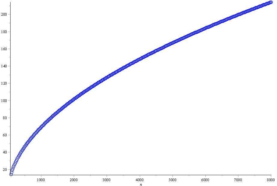
Figure 1: The graph of the data $\left(n,\ln h(n)\right)$

Actually, it is very difficult to find directly a simple function to fit the data on Figure 1 with high accuracy. The main reason is that the fitting functions obtained by the methods used frequently could not reach satisfying accuracy.

Since we have several accurate estimation formula of $p(n)$ (refer [1]), such as

$$R^{\prime}_{\mathrm{h2}}(n)=\left\lfloor\frac{\exp\left(\sqrt{\frac{2}{3}}\pi\sqrt{n}\right)}{4\sqrt{3}\left(n+a_{2}\sqrt{n+c_{2}}+b_{2}\right)}+\frac{1}{2}\right\rfloor,\ (n\geqslant 80)$$

and

$$R^{\prime}_{\mathrm{h0}}(n)=\left\lfloor\frac{\exp\left(\sqrt{\frac{2}{3}}\pi\sqrt{n}\right)}{4\sqrt{3}\left(n+C^{\prime}_{2}(n)\right)}+\frac{1}{2}\right\rfloor,\quad 1\leqslant n\leqslant 100,$$

where $a_{2}=0.4432884566$, $b_{2}=0.1325096085$, $c_{2}=0.274078$ and

$$C^{\prime}_{2}(n)=\begin{cases}0.4527092482\times\sqrt{n+4.35278}-\\ \quad 0.05498719946,\quad\ n=3,5,7,\cdots,99;\\ 0.4412187317\times\sqrt{n-2.01699}+\\ \quad 0.2102618735,\quad\quad n=4,6,8\cdots,100.\end{cases}$$ (15)

By Equation (13), we can obtain $h(n)$ by

$$h_{1}(n)=\begin{cases}R^{\prime}_{\mathrm{h0}}(n)-R^{\prime}_{\mathrm{h0}}(n-1),&2\leqslant n\leqslant 80;\\ R^{\prime}_{\mathrm{h2}}(n)-R^{\prime}_{\mathrm{h2}}(n-1),&n>80.\end{cases}$$ (16)

and the error of this formula will not exceed twice of the error of $R^{\prime}_{\mathrm{h2}}(n)$ or $R^{\prime}_{\mathrm{h0}}(n)$. Of course, this formula is not as simple as we want, but the accuracy is very good.

3.1 Asymptotic Formula

As $h(n)=p(n)-p(n-1)$, by Hardy-Ramanujan’s asymptotic formula

$$p(n)\sim\frac{1}{4n\sqrt{3}}\exp\left(\sqrt{\frac{2}{3}}\pi\sqrt{n}\right)$$

(refer [31], [32], [33], [34], [3], [35], [1]), we assume that, when $n\gg 1$,
$h(n)$ $\sim$ $\frac{\exp\left(\sqrt{\frac{2}{3}}\pi\sqrt{n}\right)}{4\sqrt{3}n}-\frac{\exp\left(\sqrt{\frac{2}{3}}\pi\sqrt{n-1}\right)}{4\sqrt{3}(n-1)}$. So,

$h(n)$ $\sim$ $\frac{\exp\left(\sqrt{\frac{2}{3}}\pi\sqrt{n-1}\right)}{4\sqrt{3}}\left(\frac{\exp\left(\pi\sqrt{\frac{2}{3}}\left(\sqrt{n}-\sqrt{n-1}\right)\right)}{n}-\frac{1}{n-1}\right)$

= $\frac{\exp\left(\sqrt{\frac{2}{3}}\pi\sqrt{n-1}\right)}{4\sqrt{3}}\left(\frac{\exp\left(\frac{\pi\sqrt{2/3}}{\sqrt{n}+\sqrt{n-1}}\right)}{n}-\frac{1}{n-1}\right)$

$\sim$ $\frac{\exp\left(\sqrt{\frac{2}{3}}\pi\sqrt{n}\right)}{4\sqrt{3}}\left(\frac{\exp\left(\frac{\pi\sqrt{2/3}}{2\sqrt{n}}\right)}{n}-\frac{1}{n-1}\right)$

$\sim$ $\frac{\exp\left(\sqrt{\frac{2}{3}}\pi\sqrt{n}\right)}{4\sqrt{3}}\left(\frac{1+\frac{\pi}{\sqrt{6n}}}{n}-\frac{1}{n-1}\right)$

$\sim$ $\frac{\exp\left(\sqrt{\frac{2}{3}}\pi\sqrt{n}\right)}{4\sqrt{3}}\left(\frac{\pi}{\sqrt{6n^{3}}}\right)$$=$ $\frac{\pi\exp\left(\sqrt{\frac{2}{3}}\pi\sqrt{n}\right)}{12\sqrt{2n^{3}}}.$

So,

$$h(n)\sim\frac{\pi}{12\sqrt{2n^{3}}}\exp\left(\sqrt{\frac{2}{3}}\pi\sqrt{n}\right).$$ (17)

Table 4: The relative error of $I_{\mathrm{g}}(n)$ to $h(n)$ when $n\leqslant 1000$.

Table 5: The relative error of $\left\lfloor I_{\mathrm{g}}(n)+\frac{1}{2}\right\rfloor$ to $h(n)$ when $n\leqslant 30$.

In coincidence, half a year after the main results were obtained in this paper, the author found an asymptotic formula

$$P_{a,b}(n)\text{$\sim$} \Gamma\left(\frac{b}{a}\right)\pi^{b/a-1}2^{-(3/2)-(b/2a)}3^{-(b/2a)}$$

$$\quad a^{-(1/2)+(b/2a)}n^{-\frac{a+b}{2a}}\mathrm{e}^{\pi\sqrt{\frac{2n}{3a}}},$$ (18)

in [30]. When $a$ = 1, $b$ = 2, we will have

$$P_{1,2}(n)\text{$\sim$}\frac{\pi}{12\sqrt{2n^{3}}}\exp\left(\pi\sqrt{\frac{2}{3}n}\right),$$ (19)

which coincides with the asymptotic formula obtained here.

The formula (17) will be called the Ingham-Meinardus asymptotic formula in this paper, since Daniel mentioned in [30] that this general asymptotic formula (18) was first given by A. E. Ingham in [29] and the proof was refined by G. Meinardus later in another two papers written in German.

Later in this paper, $\frac{\pi}{12\sqrt{2n^{3}}}\exp\left(\sqrt{\frac{2}{3}}\pi\sqrt{n}\right)$ will be denoted by $I_{\mathrm{g}}(n)$ for short.

It is not satisfying to estimate $h(n)$ by $I_{\mathrm{g}}(n)$ when $n$ is small. The relative error of $I_{\mathrm{g}}(n)$ to $h(n)$ is greater than 6% as shown on Table 5 (on page 5). The round approximation

$$I^{\prime}_{\mathrm{g}}(n)=\left\lfloor I_{\mathrm{g}}(n)+\frac{1}{2}\right\rfloor$$

will not change the accuracy distinctly, as shown on Table 5 (on page 5). So it is necessary to modify the asymptotic formula for better accuracy.

3.2 Method A: Modifying the exponent

In this subsection we consider fitting $h(n)$ by $I_{\mathrm{ga}}=\frac{\pi}{12\sqrt{2n^{3}}}\exp\left(\sqrt{\frac{2}{3}}\pi\sqrt{n+C_{1}(n)}\right)$, or fitting
$\left(n,\,\frac{3}{2\pi^{2}}\left(\ln\left(\frac{12\sqrt{2n^{3}}h(n)}{\pi}\right)\right)^{2}-n\right)$ ( $n$ = $60+20k$, $k$ = 1, 2, $\cdots$, 397) by a function

$$f_{1}(x)\doteq\frac{a_{1}}{\left(x+c_{1}\right)^{e_{1}}}+b_{1},$$ (20)

Let $C_{1}(n)$ = $\frac{3}{2\pi^{2}}\left(\ln\left(\frac{12\sqrt{2n^{3}}h(n)}{\pi}\right)\right)^{2}-n$. The reason that we fit $C_{1}(x)$ by the function in the form displayed in (20) is the same as that described in section 3 of [1] (although the data differs distinctly). Many other types of functions have been tested, but they can not fit these data very well.

But here it is not valid to obtain the constants in $f_{1}(n)$ by iteration method described in reference [1].

The figure of the data $\left(n,\,\frac{3}{2\pi^{2}}\left(\ln\left(\frac{12\sqrt{2n^{3}}h(n)}{\pi}\right)\right)^{2}-n\right)$ ( $n$ = $60+20k$, $k$ = 1, 2, $\cdots$, 397) is shown on Figure 2 on page 2.

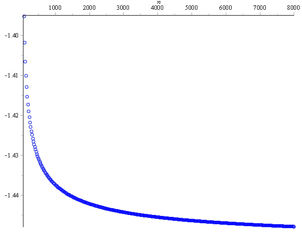
Figure 2: The graph of the data $\left(n,\frac{3}{2\pi^{2}}\left(\ln\left(\frac{12\sqrt{2n^{3}}h(n)}{\pi}\right)\right)^{2}-n\right)$

First, we try to fit $\left(n,\,\frac{3}{2\pi^{2}}\left(\ln\left(\frac{12\sqrt{2n^{3}}h(n)}{\pi}\right)\right)^{2}-n\right)$ ( $n$ = $60+20k$, $k$ = 1, 2, $\cdots$, 397) by a function in the form

$$f_{1}(x)\doteq\frac{a_{1}}{\sqrt{x+c_{1}}}+b_{1}.$$ (21)

That means we have assumed that $e_{1}=1/2$, temporarily. We will explain the reason in subsection 3.2.3.

The average error of $f_{1}(x)$ is

$$E_{1}= \sqrt{\frac{1}{K_{1}}\sum\limits_{n}\left(C_{1}(n)-f_{1}(n)\right)^{2}}$$ (22)

$$= \sqrt{\frac{1}{K_{1}}\sum\limits_{n}\left(C_{1}(n)-\frac{a_{1}}{\sqrt{n+c_{1}}}-b_{1}\right)^{2}}$$

$E_{1}=\sqrt{\frac{1}{K_{1}}\sum\limits_{k=1}^{K_{1}}\left(C_{1}(60+20k)-\frac{a_{1}}{\sqrt{60+20k+c_{1}}}-b_{1}\right)^{2}}$,
where $K_{1}$ = 397, $n$ ranges from 80 to 8000, by step 20. Here only $a_{1}$, $b_{1}$, and $c_{1}$ are unknown, so we can consider $E_{1}$ as a function of the variables $\left(a_{1},b_{1},c_{1}\right)$.

We want to find a triple $\left(a_{1},b_{1},c_{1}\right)$ such that $E_{1}$ reaches its minimum, or to make $E_{1}$ as small as possible.

Since a lot of functions have several local minimum points, it is necessary to find out whether $E_{1}$ = $E_{1}\left(a_{1},b_{1},c_{1}\right)$ has more than one local minimum before we start to calculate the minimum point by numeral method. But $E_{1}$ = $E_{1}\left(a_{1},b_{1},c_{1}\right)$ is too complicate, it is very difficult to know all the critical points in the range we are considering.

3.2.1 Preparation work

For a given pair $\left(a_{1},c_{1}\right)$, by the property of the arithmetic mean, it is clear that $E_{1}$ reaches its minimum when

$$b_{1} =\frac{1}{K_{1}}\sum\limits_{n}\left(C_{1}(n)-\frac{a_{1}}{\sqrt{n+c_{1}}}\right)$$

$$=\overline{C_{1}}-\frac{1}{K_{1}}\sum\limits_{n^{\prime}}\frac{a_{1}}{\sqrt{n^{\prime}+c_{1}}},$$ (23)

where $\overline{C_{1}}$ = $\frac{1}{K_{1}}\sum\limits_{n^{\prime}}C_{1}(n^{\prime})$.

Let
$E_{1}=\sqrt{\frac{1}{K_{1}}\sum\limits_{n}\left(C_{1}(n)-\frac{a_{1}}{\sqrt{n+c_{1}}}-\overline{C_{1}}+\frac{1}{K_{1}}\underset{{}_{n^{\prime}}}{\sum}\frac{a_{1}}{\sqrt{n^{\prime}+c_{1}}}\right)^{2}}$ be the average error of the the fitting function $f_{1}(x)\doteq\frac{a_{1}}{\sqrt{x+c_{1}}}+\overline{C_{1}}-\frac{1}{K_{1}}\sum\limits_{n^{\prime}}\frac{a_{1}}{\sqrt{n^{\prime}+c_{1}}}$. (Here $a_{1}$ and $b_{1}$ are undetermined coefficients.)

Let $G_{1}=E_{1}^{2}=$
$\frac{1}{K_{1}}\sum\limits_{n}\left(C_{1}(n)-\frac{a_{1}}{\sqrt{n+c_{1}}}-\overline{C_{1}}+\frac{1}{K_{1}}\sum\limits_{n^{\prime}}\frac{a_{1}}{\sqrt{n^{\prime}+c_{1}}}\right)^{2}.$ Here only $a_{1}$ and $b_{1}$ are unknowns. $G_{1}$ could be considered as a function of $\left(a_{1},c_{1}\right)$. In order to find the minimum point of $G_{1}$, we can draw the figure of the function $G_{1}=G_{1}\left(a_{1},c_{1}\right)$, (In a cube coordinate system with axis $a_{1},c_{1}$ and $G_{1}$) as shown on Figure 6, Figure 6 and Figure 10. Figure 6 and Figure 6 are the projection of the graph of $\left(a_{1},c_{1},G_{1}\right)$ (when $-100$ $\leqslant$ $a_{1}$ $\leqslant$ 100, $-50$ $\leqslant$ $c_{1}$ $\leqslant$ 100, which is a part of a surface) on the $a_{1}-G_{1}$ plane (spanned by the axis $a_{1}$ and $G_{1}$) and $c_{1}-G$ plane, respectively.

From these figures, we can find out that the influence of $c_{1}$ to $G_{1}$ is much less than that of $a_{1}$. In Figure 10, we find that when $G_{1}$ reaches its minimum, $a_{1}$ is between 0.50 and 0.53, but there is not a definite range for $c_{1}$.

It is possible that for different range of $c_{1}$, the range of $a_{1}$ when $G_{1}$ reaches its minimum will be different. But considering that $\frac{a_{1}}{\sqrt{n+c_{1}}}+b_{1}$ is a real, $c_{1}$ should be greater than $-1$ in theory. (For the fitting data used here, $c_{1}$ should be greater than $-80$.) From Figure 6, we can see that $G_{1}$ touches its bottom when $-15$ $\leqslant$ $a_{1}$ $\leqslant$ 15. Although we can not see clearly the exact value of of $a_{1}$ in the minimum points, we can draw another figure of $\left(a_{1},c_{1},G_{1}\right)$ when $-15$ $\leqslant$ $a_{1}$ $\leqslant$ 15 and $-1$ $\leqslant$ $c_{1}$ $\leqslant$ 100 to observe more details (the figure is not presented here), then we will find that the more detailed range of $a_{1}$ for the minimum points is $[-3,3]$ in the new figure (not presented), next, draw the figures of $\left(a_{1},c_{1},G_{1}\right)$ when $-3$ $\leqslant$ $a_{1}$ $\leqslant$ 3, $0$ $\leqslant$ $a_{1}$ $\leqslant$ 1, $0.2$ $\leqslant$ $a_{1}$ $\leqslant$ 0.8 or $0.45$ $\leqslant$ $a_{1}$ $\leqslant$ 0.6, respectively, while $-1$ $\leqslant$ $c_{1}$ $\leqslant$ 100, we will find the range of $a_{1}$ of the minimum points of $G_{1}$ is about [0.50, 0.53]. The projections of the figure 10 of $\left(a_{1},c_{1},G_{1}\right)$ when $0.45$ $\leqslant$ $a_{1}$ $\leqslant$ 0.6 and $-1$ $\leqslant$ $c_{1}$ $\leqslant$ 100 is shown on Figure 10 and Figure 10.

In Figure 6, for the curves on the bottom, $G_{1}$ decrease with $c_{1}$ at first then increases with $c_{1}$, but it is difficult to find the critical point in the figure, since different curves have different critical points.

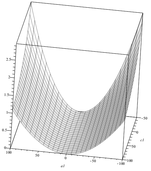
Figure 3: The graph of the data $\left(a_{1},c_{1},G_{1}\right)$ when $-100$ $\leqslant$ $a_{1}$ $\leqslant$ 100, $-50$ $\leqslant$ $c_{1}$ $\leqslant$ 100

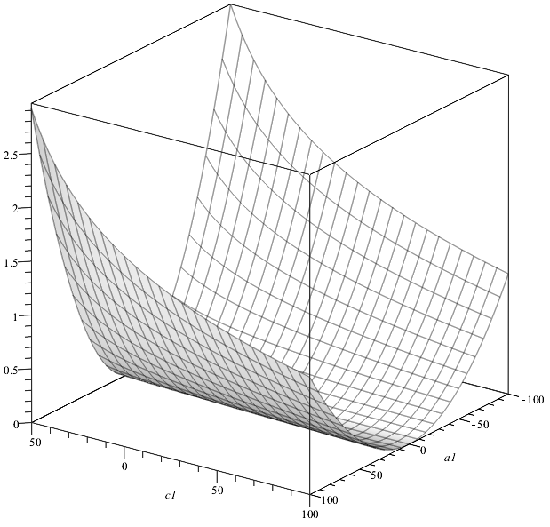
Figure 4: The graph of the data $\left(a_{1},c_{1},G_{1}\right)$ when $-100$ $\leqslant$ $a_{1}$ $\leqslant$ 100, $-50$ $\leqslant$ $c_{1}$ $\leqslant$ 100 version 2

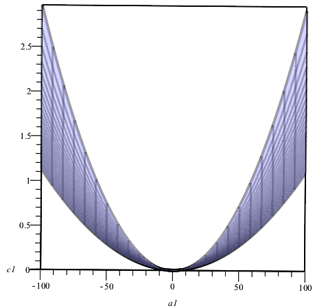
Figure 5: The projection of the graph of the data $\left(a_{1},c_{1},G_{1}\right)$ on the $a_{1}-G_{1}$ plane when $-100$ $\leqslant$ $a_{1}$ $\leqslant$ 100, $-50$ $\leqslant$ $c_{1}$ $\leqslant$ 100

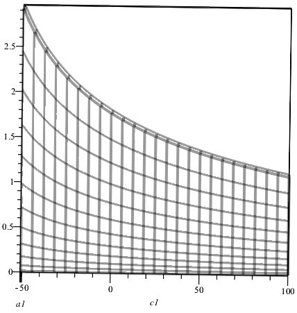
Figure 6: The projection of the graph of the data $\left(a_{1},c_{1},G_{1}\right)$ on the $c_{1}-G_{1}$ plane when $-100$ $\leqslant$ $a_{1}$ $\leqslant$ 100, $-50$ $\leqslant$ $c_{1}$ $\leqslant$ 100

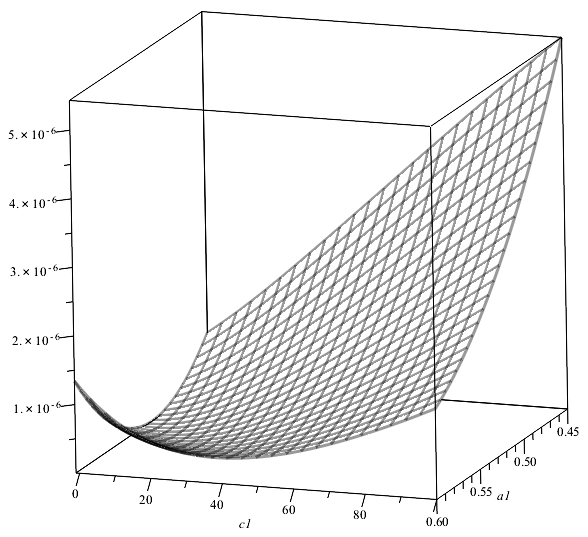
Figure 7: The graph of the data $\left(a_{1},c_{1},G_{1}\right)$ when $0.45$ $\leqslant$ $a_{1}$ $\leqslant$ 0.60, $-1$ $\leqslant$ $c_{1}$ $\leqslant$ 100

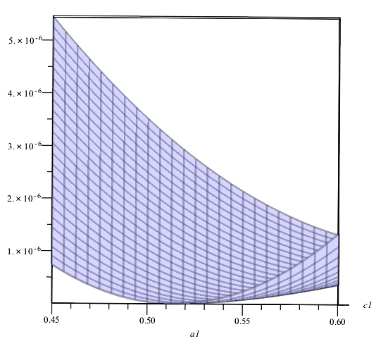
Figure 8: The projection of the graph of the data $\left(a_{1},c_{1},G_{1}\right)$ on the $a_{1}-G_{1}$ plane when $0.45$ $\leqslant$ $a_{1}$ $\leqslant$ 0.60, $-1$ $\leqslant$ $c_{1}$ $\leqslant$ 100

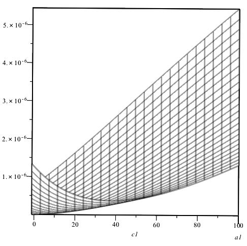
Figure 9: The projection of the graph of the data $\left(a_{1},c_{1},G_{1}\right)$ on the $c_{1}-G_{1}$ plane when $0.45$ $\leqslant$ $a_{1}$ $\leqslant$ 0.60, $-1$ $\leqslant$ $c_{1}$ $\leqslant$ 100

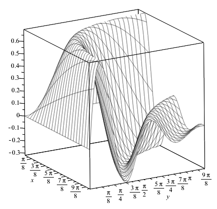
Figure 10: Example of a surface with more than one bottom.

Although we can not find an satisfying value of $a_{1}$ or $c_{1}$ from the figures above to construct a fitting function $f_{1}$, these pictures show that the figure of $G_{1}=\left(a_{1},c_{1},G_{1}\right)$ has only one bottom in the domain we are considering, unlike the figure of another function shown on Figure 10, so the existence of the minimum point is almost confirmed, therefore we are confident to find the value of $a_{1}$ or $c_{1}$ in the minimum point by numerical method. This guarantees the validity of the numerical calculation by loop in next step.

3.2.2 Find $c_{1}$

On the other hand, by the least square method, to fit the data $\left(x_{k},\,y_{k}\right)$ ($k$ = 1, 2, $\cdots$, $K_{1}$) by a linear function $y=a\times x+b$, the result is that

$$a = \frac{\overline{x_{n}\cdot y_{n}}-\overline{x_{n}}\cdot\overline{y_{n}}}{\overline{x_{n}^{2}}-\left(\overline{x_{n}}\right)^{2}},$$ (24)

$$b = \frac{\overline{x_{n}}\cdot\overline{x_{n}\cdot y_{n}}-\overline{x_{n}^{2}}\cdot\overline{y_{n}}}{\left(\overline{x_{n}}\right)^{2}-\overline{x_{n}^{2}}}=\overline{y_{n}}-\overline{x_{n}}\cdot a,$$ (25)

where $\overline{x_{n}}$ = $\frac{1}{K_{1}}\sum\limits_{i=1}^{K_{1}}x_{i}$ is the average value of $x_{i}$, $\overline{y_{n}}$ = $\frac{1}{K_{1}}\sum\limits_{i=1}^{K_{1}}y_{i}$, $\overline{x_{i}^{2}}$ = $\frac{1}{K_{1}}\sum\limits_{i=1}^{K_{1}}x_{i}^{2}$, $\overline{x_{n}\cdot y_{n}}$ = $\frac{1}{K_{1}}\sum\limits_{i=1}^{K_{1}}x_{i}\cdot y_{i}$. By definition, $\left(\overline{x_{n}}\right)^{2}$ = $\left(\frac{1}{K_{1}}\sum\limits_{i=1}^{K_{1}}x_{i}\right)^{2}$ is the square of the average value of $x_{n}$. So, by the least square method, $a$ and $b$ are uniquely determined by the given data $\left(x_{k},\,y_{k}\right)$ ($k$ = 1, 2, $\cdots$, $K_{1}$).

For every given value of $c_{1}$ (greater than $-80$), we can fit $\left(n,\,C_{1}(n)\right)$ ($n$ = $60+20k$, $k$ = 1, 2, $\cdots$, 397) by a function $f_{1}(x)\doteq\frac{a_{1}}{\sqrt{x+c_{1}}}+b_{1}$ by the least square method, if we consider $\frac{1}{\sqrt{60+20k+c_{1}}}$ and $C_{1}(60+20k)$ as $x_{k}$ and $y_{k}$, respectively. Then

$\overline{x_{n}}$ = $\frac{1}{K_{1}}\sum\limits_{k=1}^{K_{1}}x_{k}$ = $\frac{1}{K_{1}}\sum\limits_{k=1}^{K_{1}}\frac{1}{\sqrt{60+20k+c_{1}}}$, $\overline{y_{n}}$ = $\frac{1}{K_{1}}\sum\limits_{k=1}^{K_{1}}y_{k}$ = $\frac{1}{K_{1}}\sum\limits_{k=1}^{K_{1}}C_{1}(60+20k)$,

$\overline{x_{n}^{2}}$ = $\frac{1}{K_{1}}\sum\limits_{k=1}^{K_{1}}x_{k}^{2}$ = $\frac{1}{K_{1}}\sum\limits_{k=1}^{K_{1}}\frac{1}{60+20k+c_{1}}$,

$\overline{x_{n}\cdot y_{n}}$ = $\frac{1}{K_{1}}\sum\limits_{k=1}^{K_{1}}x_{k}\cdot y_{k}$ = $\frac{1}{K_{1}}\sum\limits_{k=1}^{K_{1}}\frac{C_{1}(60+20k)}{\sqrt{60+20k+c_{1}}}$,

$a_{1}=\frac{\overline{x_{n}\cdot y_{n}}-\overline{x_{n}}\cdot\overline{y_{n}}}{\overline{x_{n}^{2}}-\left(\overline{x_{n}}\right)^{2}}$,     $b_{1}=\overline{y_{n}}-\overline{x_{n}}\cdot a_{1}$.

So $a_{1}$ and $b_{1}$ could both be considered as functions of $c_{1}$, denoted by $a_{1}=a_{1}(c_{1})$, $b_{1}=b_{1}(c_{1})$, since they are uniquely determined by $c_{1}$ with the given data.

Then $G_{2}=E_{1}^{2}=$
$\frac{1}{K_{1}}\sum\limits_{k=1}^{K_{1}}\left(C_{1}(60+20k)-\frac{a_{1}(c_{1})}{\sqrt{60+20k+c_{1}}}-b_{1}(c_{1})\right)^{2}$ is a function of $c_{1}$.

It will cost some time to plot the figure of the function $G_{2}$ = $G_{2}(c_{1})$ in a CAS software.

If we plot the figure of the function $G_{2}$ = $G_{2}(c_{1})$ on the coordinates (as shown on Figure 13, Figure 13 and Figure 13), we will find that $G_{2}$ reaches its minimum when $c_{1}$ $\approx$ $-3.2594807$. On Figure 13, we find that the curve of $G_{2}$ = $G_{2}(c_{1})$ is not so smooth. The reason is that we hold up 18 significant digits in the process. If we compute more significant digits in the process, the curve on Figure 13 will be more smooth, at the cost of much more time. By writing a small program (since the default function to find the minimum provide by the software Maple 18 are unable to deal with such a complicated function $G_{2}$ = $G_{2}(c_{1})$ involving so much data), we can obtain a more accurate value of the critical point

$$c_{1}=-3.259480684.$$

When the value of $c_{1}$ is obtained, we can find the value of $a_{1}$ and $b_{1}$ by the least square method without difficulty, i.e.,

$$a_{1} =0.5097429624,$$

$$b_{1} =-1.453552800.$$

But here $c_{1}$ is less than $-1$, so the estimation formula for $h(n)$ constructed from these coefficients is invalid when $n<4$.

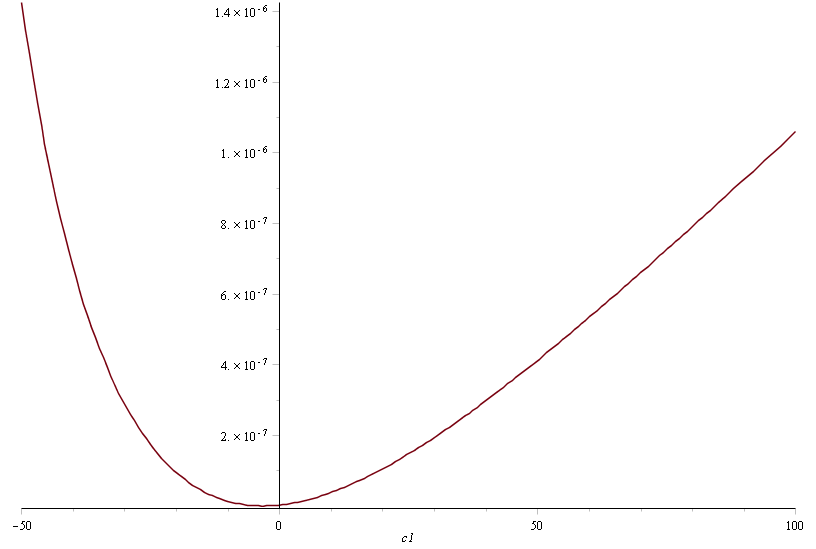
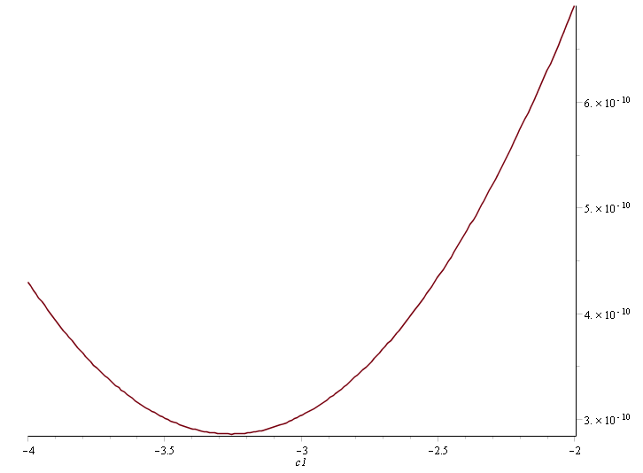
Figure 11: The graph of the function $G_{2}$ = $G_{2}(c_{1})$ when $-50$ $\leqslant$ $c_{1}$ $\leqslant$ 100

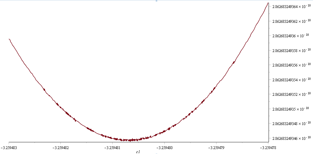
Figure 12: The graph of the function $G_{2}$ = $G_{2}(c_{1})$ when $-4$ $\leqslant$ $c_{1}$ $\leqslant$ -2

Figure 13: The graph of the function $G_{2}$ = $G_{2}(c_{1})$ when $-3.259483$ $\leqslant$ $c_{1}$ $\leqslant$ $-3.259478$

3.2.3 Confirm $e_{1}$

In [1] we fit $C_{1}(n)$ = $\frac{3}{2}\cdot\frac{\left(\ln\left(4n\sqrt{3}p(n)\right)\right)^{2}}{\pi^{2}}-n$ by by a function $f_{1}(x)\doteq\frac{a_{1}}{\left(n+c_{1}\right)^{e_{1}}}+b_{1}$ when estimating $p(n)$, and found that $e_{1}$ $\approx$ $0.50$ by iteration. Here the iteration method does not work well, so we fit $C_{1}(n)$ = $\frac{3}{2\pi^{2}}\left(\ln\left(\frac{12\sqrt{2n^{3}}h(n)}{\pi}\right)\right)^{2}-n$ by a function $f_{1}(x)\doteq\frac{a_{1}}{\sqrt{n+c_{1}}}+b_{1}$ directly, which means that we have assumed that $e_{1}$ $=$ $\frac{1}{2}$. Here we may doubt that whether $e_{1}$ $=$ $0.5$ is the best option for us?

Here we use the same idea described in subsection 3.2.1.

For every pair $(e_{1},c_{1})$, we can obtain corresponding $a_{1}$ and $b_{1}$ by the least square method, just like (24) and (25), except that here $x_{k}=\frac{1}{\left(60+20k+c_{1}\right)^{e_{1}}}$.

So the square of the average error
$G_{3}=E_{1}^{2}=\frac{1}{K_{1}}\sum\limits_{n}\left(C_{1}(n)-\frac{a_{1}\left(e_{1},c_{1}\right)}{\left(n+c_{1}\right)^{e_{1}}}-b_{1}\left(e_{1},c_{1}\right)\right)^{2}$
could be considered as a function of $e_{1}$ and $c_{1}$, as both $a_{1}=a_{1}\left(e_{1},c_{1}\right)$ and $b_{1}=b_{1}\left(e_{1},c_{1}\right)$ could be expressed by certain elementary functions of $e_{1}$ and $c_{1}$.

If we draw the figure of the function $G_{3}$ = $G_{3}(e_{1},c_{1})$, we will find that the surface has only one bottom when $0.1$ $\leqslant$ $e_{1}$ $\leqslant$ $0.9$, $-50$ $\leqslant$ $c_{1}$ $\leqslant$ $100$, as shown on Figure 14. But the process to draw the figure is time-consuming. It costs more than 5 hours on a notebook (ThinkPad E40 Edge, with 6 GB RAM and AMD P360 Dual-Core Processor 2.30GHz) by Maple 18 in Ubuntu 14.04.1 system.

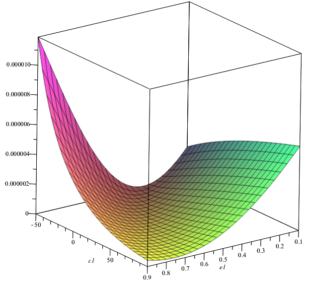
Figure 14: The graph of the function $G_{3}$ = $G_{3}(e_{1},c_{1})$ when $0.1$ $\leqslant$ $e_{1}$ $\leqslant$ $0.9$, $-50$ $\leqslant$ $c_{1}$ $\leqslant$ $100$

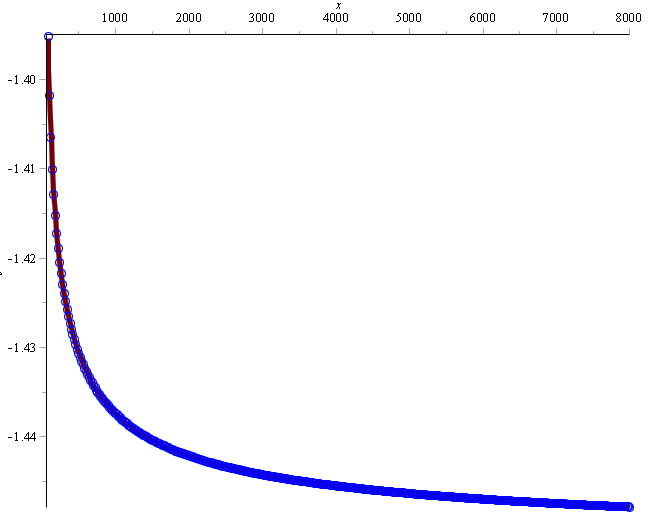
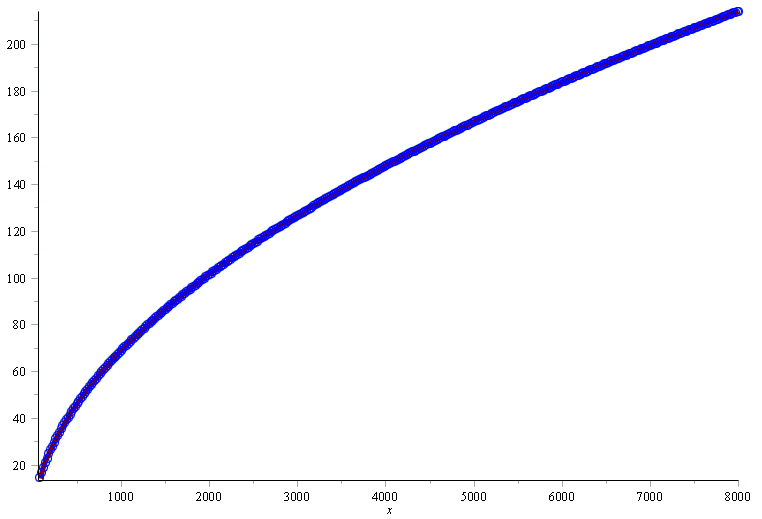
Figure 15: The graph of the data $\left(n,\frac{3}{2\pi^{2}}\left(\ln\left(\frac{12\sqrt{2n^{3}}h(n)}{\pi}\right)\right)^{2}-n\right)$ and the fitting curve

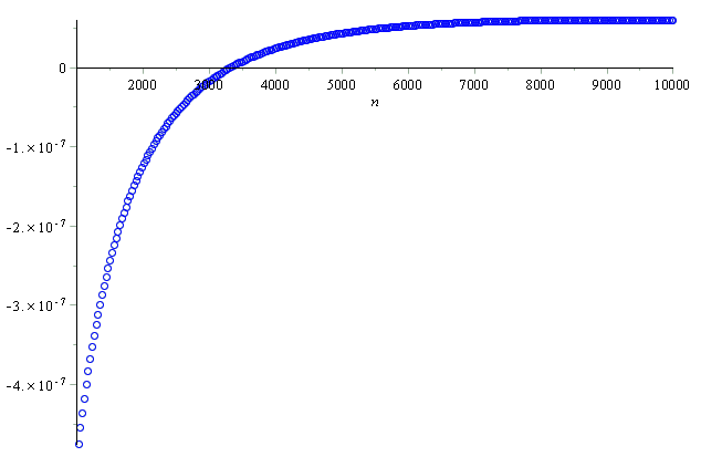
Figure 16: The graph of the data $\left(n,\ln\left(h(n)\right)\right)$ and the fitting curve

Figure 17: The Relative Error of $I_{\mathrm{ga}}(n)$when 1000 $\leqslant$ $n$ $\leqslant$ 10000, step 300

After that, by written another program, we can obtain the approximate value of $(e_{1},c_{1})$ where $G_{3}$ touches the bottom, i.e. $e_{1}$ $\approx$ $0.494$, $c_{1}$ $\approx$ $-4.85$, when 18 significant digits are involved in the process, which still costs tens of minutes. Considering that we have used only a small part of data, we can not afford the time for computing more significant digits in process, and the computing is so complicated hence error accumulation effect is considerable, so we choose $e_{1}$ $=$ $0.50$ while it differs very little with $0.494$. Another reason is that we prefer simple exponent, as the time spend on computing a square root is much less than that to compute a power with exponent $0.494$ in general. Here the value of $c_{1}\approx-4.85$ is obviously different from the value obtained at the end of subsection (3.2.2), because of the little difference on $e_{1}$. Therefore, it will be fine to use the result in subsection (3.2.2).

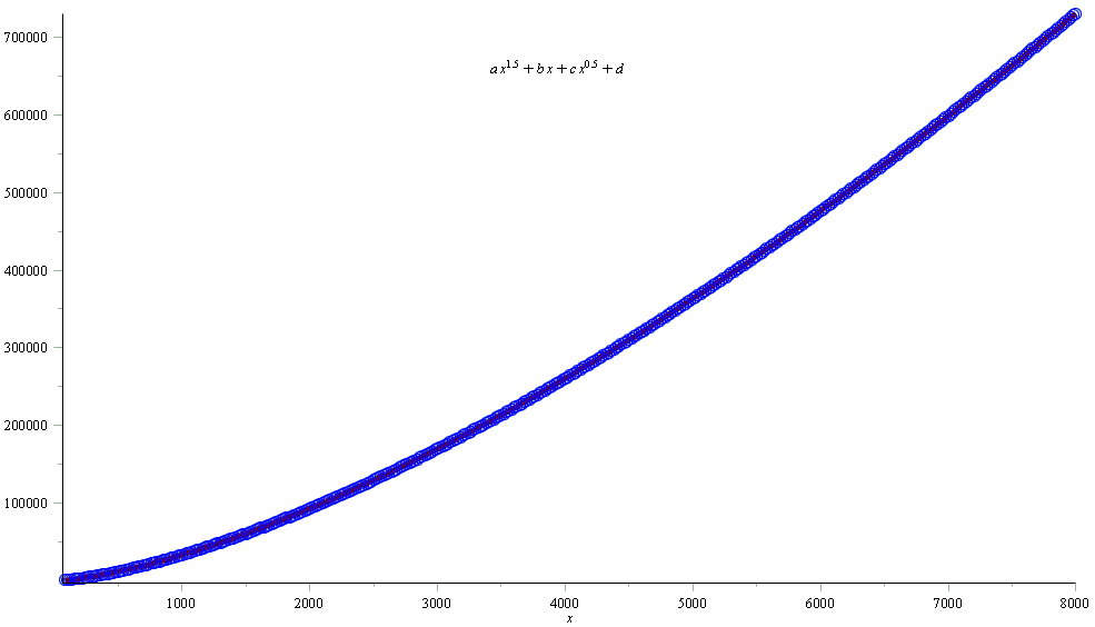
Figure 18: The graph of the data $\Bigl{(}n,\,\frac{\pi\exp\left(\pi\sqrt{\frac{2}{3}}\sqrt{n}\right)}{12\sqrt{2}h(n)}\Bigr{)}$ and the fitting curve

In this figure, the points are shown as small circles which are very close to each other. Theses crowded circles seams like a thick curve. A fitting curve passes though the center of these circles. The fitting curve might not be found in reduce printing. That means the curve fits the points (displayed as circles) very well.

3.2.4 The Result

By the value $a_{1}$ = 0.5097429624, $b_{1}$ = $-$1.453552800, $c_{1}$ = $-3.259480684$ obtained in subsection 3.2.2, we will have a fitting function
$f_{1}(x)\doteq\frac{a_{1}}{\sqrt{x+c_{1}}}+b_{1}$.
The figure of $f_{1}(x)$ (when $-80$ $\leqslant$ $x$ $\leqslant$ 8000) together with the figure of the data $\left(n,\,\frac{3}{2\pi^{2}}\left(\ln\left(\frac{12\sqrt{2n^{3}}h(n)}{\pi}\right)\right)^{2}-n\right)$ ( $n$ = $60+20k$, $k$ = 1, 2, $\cdots$, 397) are shown on Figure 17. It shows that $f_{1}(n)$ fits $\frac{3}{2\pi^{2}}\left(\ln\left(\frac{12\sqrt{2n^{3}}h(n)}{\pi}\right)\right)^{2}-n$ very well.

Then we could fit $h(n)$ by

$$I_{\mathrm{ga}}(n)=\frac{\pi\exp\left(\sqrt{\frac{2}{3}}\pi\sqrt{n+\frac{a_{1}}{\sqrt{x+c_{1}}}+b_{1}}\right)}{12\sqrt{2n^{3}}},\quad n\geqslant 4.$$ (26)

The figure of the function $\ln\left(I_{\mathrm{ga}}(x)\right)$ together with the figure of the data $\left(n,\ln\left(h(n)\right)\right)$ ( $n$ = $60+20k$, $k$ = 1, 2, $\cdots$, 397) are shown on Figure 17. It seems that $I_{\mathrm{ga}}(n)$ fits $h(n)$ very well.

The relative error of $I_{\mathrm{ga}}$ is shown on Table 7 (when $n\leqslant 1000$ ) and Figure 17 (when 1000 $<$ $n$ $\leqslant 10000$).

When $n<20$, the relative error of $I_{\mathrm{ga}}$ is still greater than $2\%$. Although it is much better than the error of $I_{\mathrm{g}}$, it is not as good as expect when $n<40$. If we take the round approximation by

$$I^{\prime}_{\mathrm{ga}}(n) =\left\lfloor\frac{\pi\exp\left(\sqrt{\frac{2}{3}}\pi\sqrt{n+\frac{a_{1}}{\sqrt{x+c_{1}}}+b_{1}}\right)}{12\sqrt{2n^{3}}}+\frac{1}{2}\right\rfloor,$$

$$\quad n\geqslant 4,$$ (27)

the relative error will be obviously smaller with a few exceptions, as shown on Table 7.

Later we will find out that it is obviously greater than the relative error of $I_{\mathrm{g1}}$ and $I_{\mathrm{g2}}$ obtained in the next subsection by modifying the denominator part; when $4000<n<10000$, the relative error of $I_{\mathrm{ga}}$ is about 1000 times of that of $I_{\mathrm{g2}}$.

Table 6: The relative error of $I_{\mathrm{ga}}(n)$ to $h(n)$ when $n\leqslant 1000$.

Table 7: The relative error of $\left\lfloor I_{\mathrm{ga}}(n)+\frac{1}{2}\right\rfloor$ to $h(n)$ when $n\leqslant 30$.

When 30 $<$ $n$ $\leqslant$ 1000, the relative error of $\left\lfloor I_{\mathrm{ga}}(n)+\frac{1}{2}\right\rfloor$ is closed to that of $I_{\mathrm{ga}}(n)$.

3.3 Method B: Modifying the Denominator

Since $h(n)$ $\sim$ $\frac{\pi}{12\sqrt{2n^{3}}}\exp\left(\sqrt{\frac{2}{3}}\pi\sqrt{n}\right)$, we consider estimating $h(n)$ by
$\frac{\pi}{12\sqrt{2C_{3}(n)}}\exp\left(\sqrt{\frac{2}{3}}\pi\sqrt{n}\right)$, (i.e., fit $\frac{\pi^{2}\exp\left(2\pi\sqrt{\frac{2}{3}}\sqrt{n}\right)}{288h^{2}(n)}$ by a function $C_{3}(n)$), where $C_{3}(x)$ is a cubic function or a function like

$$ax^{3}+bx^{2.5}+cx^{2}+dx^{1.5}+ex+fx^{0.5}+g.$$

But the results are worse, as the relative errors are obviously much greater than the relative error of $I_{\mathrm{g}}(n)$ when $n<350$.

Then we consider estimating $h(n)$ by $\frac{\pi}{12\sqrt{2}C_{4}(n)}\exp\left(\sqrt{\frac{2}{3}}\pi\sqrt{n}\right)$, or fit $\frac{\pi\exp\left(\pi\sqrt{\frac{2}{3}}\sqrt{n}\right)}{12\sqrt{2}h(n)}$ by a function

$$C_{4}(n)=a_{4}n^{1.5}+b_{4}n+c_{4}n^{0.5}+d_{4}.$$ (28)

The result is very good. The figure of the data $\left(n,\,\frac{\pi\exp\left(\pi\sqrt{\frac{2}{3}}\sqrt{n}\right)}{12\sqrt{2}h(n)}\right)$ and the fitting curve $C_{4}(n)$ are shown on Figure 18 on page 18. Here the fitting curve is displayed by a thick continuous curve, which lies in the middle of the area the circles occupied. Since the circles are too crowded, the circles themselves look like a very thick curve.

Table 8: The relative error of $I_{\mathrm{g1}}(n)$ to $h(n)$ when $n\leqslant 1000$.

Table 9: The relative error of $\left\lfloor I_{\mathrm{g1}}(n)+\frac{1}{2}\right\rfloor$ to $h(n)$ when $n\leqslant 30$.

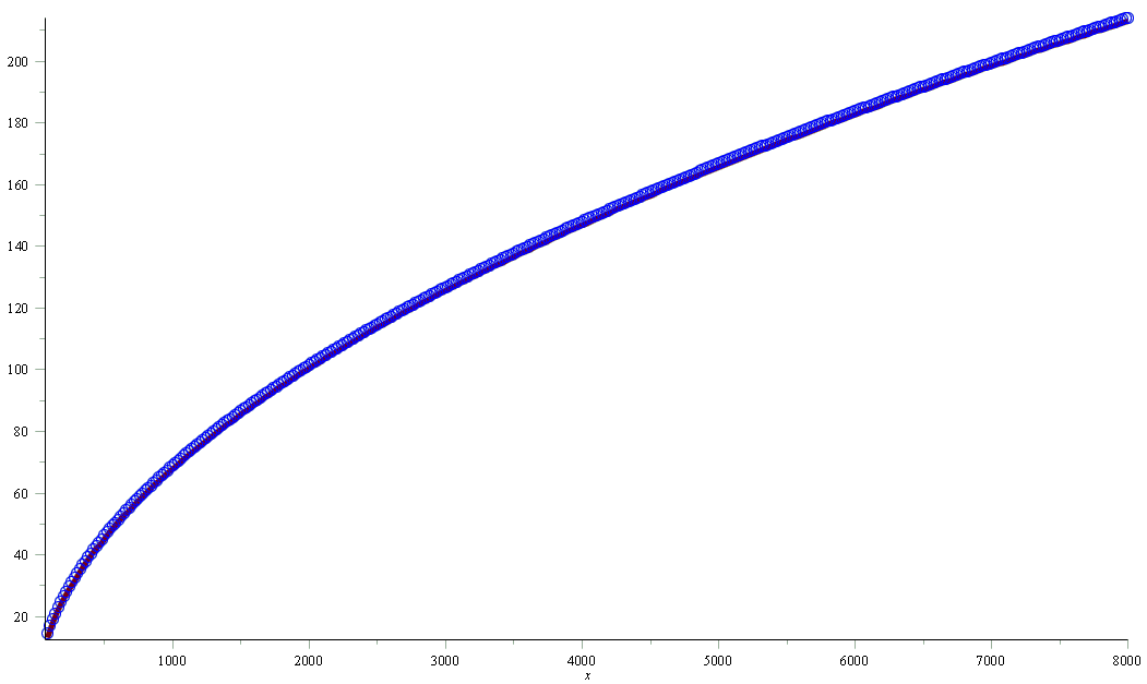
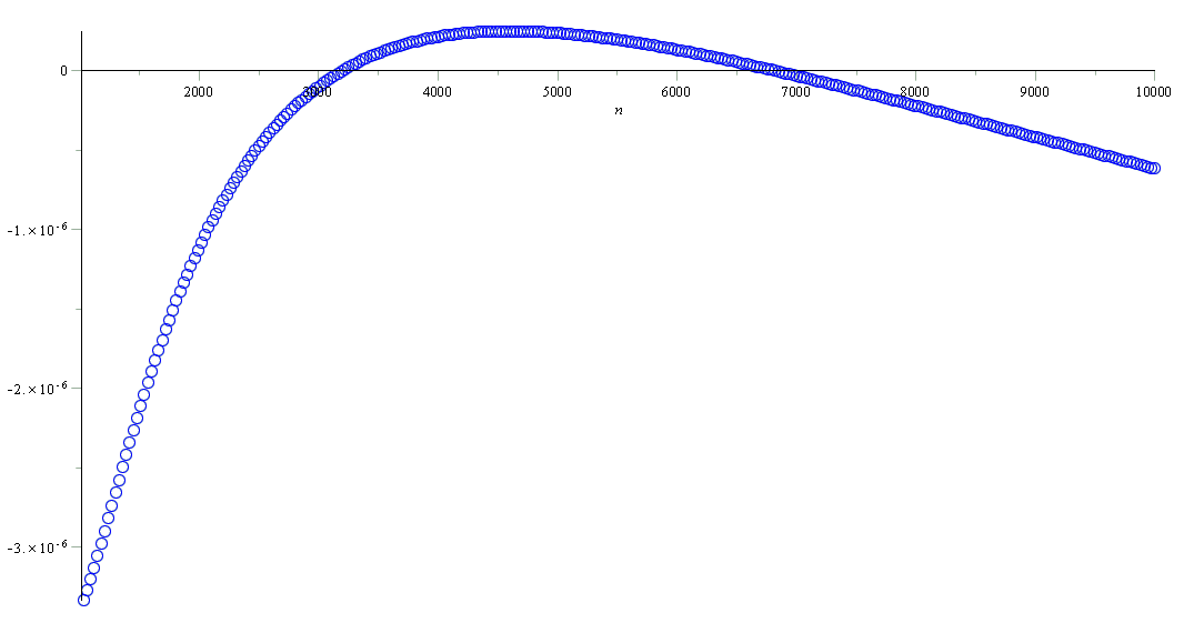
Figure 19: The graph of the data $\left(n,\ln h(n)\right)$ and the fitting curve $\ln\left(I_{\mathrm{g}1}(n)\right)$

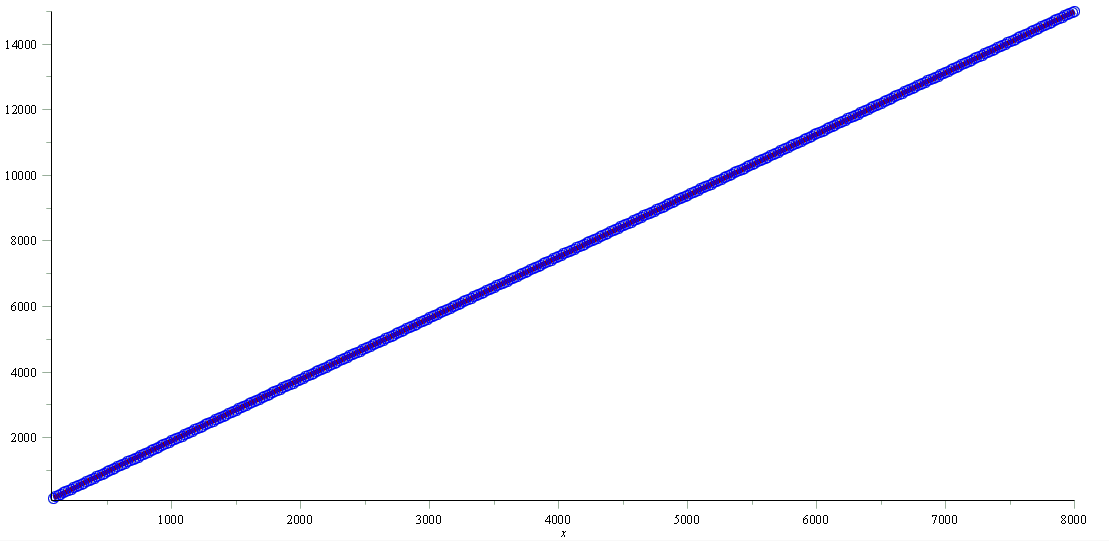
Figure 20: The Relative Error of $I_{\mathrm{g1}}(n)$when 1000 $\leqslant$ $n$ $\leqslant$ 10000, step 300

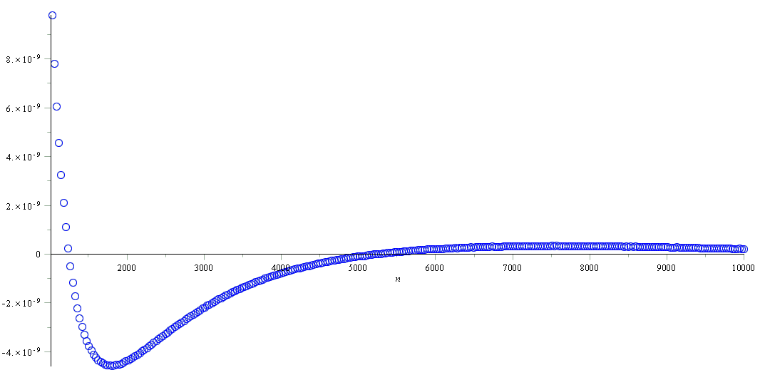
Figure 21: The graph of the data $\left(n,\ \frac{\pi\exp\left(\pi\sqrt{\frac{2}{3}}\sqrt{n}\right)}{12\sqrt{2}h(n)}-n^{3/2}\right)$ and the fitting curve $C_{5}(n)$

Figure 22: The Relative Error of $I_{\mathrm{g2}}(n)$when 1000 $\leqslant$ $n$ $\leqslant$ 10000, step 300

The values of the coefficients in the expression of $C_{4}(n)$ are as follow,

$$a_{4}= 1.000010809,$$

$$b_{4}= 1.862505234,$$

$$c_{4}= 1.169930087,$$

$$d_{4}= -0.7005460222.$$

The value of $a_{4}$ is very close to 1, which means that this fitting function coincides with the Ingham-Meinardus asymptotic formula very well.

So we have an estimation formula

$$h(n)\sim I_{\mathrm{g1}}(n)=\frac{\pi}{12\sqrt{2}C_{4}(n)}\exp\left(\sqrt{\frac{2}{3}}\pi\sqrt{n}\right).$$ (29)

We may call it the Ingham-Meinardus revised estimation formula 1. The graph of $\ln\left(I_{\mathrm{g1}}(n)\right)$ is shown on Figure 22 on page 22, together with the data points of $\left(n,\ln h(n)\right)$. This revised estimation formula is much more accurate than the asymptotic formula. The relative error is less than $1\times 10^{-6}$ when $n$ > 2000 (as shown on Figure 22 on page 22), and less than $3\permil$ when $n$ $\geqslant$ 30 (as shown on Table 9 on page 9). The relative error of the round approximation $I^{\prime}_{\mathrm{g1}}(n)=\left\lfloor I_{\mathrm{g1}}(n)+\frac{1}{2}\right\rfloor$ is shown on Table 9 on page 9.

But Equation (29) is not so satisfying when $n<30$, especially when $n<15$ as the relative error is not negligible for some value of $n$.

As we already know that $h(n)\sim\frac{\pi}{12\sqrt{2n^{3}}}\exp\left(\sqrt{\frac{2}{3}}\pi\sqrt{n}\right)$, or
   $n^{3/2}\sim\frac{\pi}{12\sqrt{2}h(n)}\exp\left(\sqrt{\frac{2}{3}}\pi\sqrt{n}\right)$, which means that when fitting $\frac{\pi\exp\left(\pi\sqrt{\frac{2}{3}}\sqrt{n}\right)}{12\sqrt{2}h(n)}$ by a function $C_{4}(n)$ shown in Equation (28), the coefficient $a_{4}$ should be exactly 1, hence we should fit $\frac{\pi\exp\left(\pi\sqrt{\frac{2}{3}}\sqrt{n}\right)}{12\sqrt{2}h(n)}$ by a function $C^{\prime}_{4}(n)=n^{3/2}+b_{5}n+c_{5}n^{1/2}+d_{5}$, or fit $\frac{\pi\exp\left(\pi\sqrt{\frac{2}{3}}\sqrt{n}\right)}{12\sqrt{2}h(n)}-n^{3/2}$ by a function

$$C_{5}(n)=b_{5}n+c_{5}n^{1/2}+d_{5}.$$ (30)

The figure of the data $\left(n,\,\frac{\pi\exp\left(\pi\sqrt{\frac{2}{3}}\sqrt{n}\right)}{12\sqrt{2}h(n)}-n^{3/2}\right)$ is shown on Figure 22 on page 22 (together with the figure of the fitting function $C_{5}(n)$ generated by the least square method).

The values of the coefficients in Equation (30) are as follow

$$b_{5}= 1.864260743,$$

$$c_{5}= 1.084436400,$$

$$d_{5}= 0.4754177757.$$

So we have another estimation formula for $h(n)$,

$$h(n)\sim I_{\mathrm{g2}}(n)=\frac{\pi\exp\left(\sqrt{\frac{2}{3}}\pi\sqrt{n}\right)}{12\sqrt{2}\left(n^{3/2}+C_{5}(n)\right)}.$$ (31)

Table 10: The relative error of $I_{\mathrm{g2}}(n)$ to $h(n)$ when $n\leqslant 1000$.

Table 11: The relative error of $\left\lfloor I_{\mathrm{g2}}(n)+\frac{1}{2}\right\rfloor$ to $h(n)$ when $n\leqslant 30$.

We may call it the Ingham-Meinardus revised estimation formula 2. The graph of $\ln\left(I_{\mathrm{g2}}(n)\right)$ is nearly the same as that of $\ln\left(I_{\mathrm{g1}}(n)\right)$ shown on Figure 22 on page 22. The second revised estimation formula is much more accurate than the first one. The relative error is less than $2\times 10^{-9}$ when $n$ > 3000 (as shown on Figure 22 on page 22), about $\frac{1}{500}$ of the relative error of $I_{\mathrm{g1}}(n)$. When $n$ < 10, the relative error is also distinctly less than that of $I_{\mathrm{g1}}(n)$ (as shown on Table 11 on page 11). The relative error of the round approximation $I^{\prime}_{\mathrm{g2}}(n)=\left\lfloor I_{\mathrm{g2}}(n)+\frac{1}{2}\right\rfloor$ is shown on Table 11 (on page 11).

It should be mentioned that in Figure 22 on page 22, the graph of the data points lie in a line, so we might be willing to fit this line by a first order equation. The result is

$$C^{\prime}_{5}(n)=1.873818457\times n+27.08318017.$$

If we use this fitting function instead of $C_{5}(n)$ generated above, the relative error to fit $h(n)$ will be about 10000 times more, that is about 20 times more than that of $I_{\mathrm{g1}}(n)$. So we did not use linear function to fit the data $\left(n,\,\frac{\pi\exp\left(\pi\sqrt{\frac{2}{3}}\sqrt{n}\right)}{12\sqrt{2}h(n)}-n^{3/2}\right)$ before.

Table 12: The relative error of $\left\lfloor F_{7a}(n)+\frac{1}{2}\right\rfloor$ to $h(n)$ when $n\leqslant 1000$.

Table 13: The relative error of $\left\lfloor F_{7b}(n)+\frac{1}{2}\right\rfloor$ to $h(n)$ when $n\leqslant 1000$.

3.4 Method C: Fittong $I_{\mathrm{g}}(n)-h(n)$

We wonder whether we can fit $I_{\mathrm{g}}(n)-h(n)$ by a function $r(n)$, then estimate $h(n)$ by $I_{\mathrm{g}}(n)-r(n)$ which may be believed more accurate than $I_{\mathrm{g2}}(n)$ at the price of being more complicated.

By the same tricks used at the beginning of this subsection, we will have

$$I_{\mathrm{g}}(n)-I_{\mathrm{g}}(n-t)\sim\frac{t\pi^{2}}{24\sqrt{3}n^{2}}\exp\left(\sqrt{\frac{2}{3}}\pi\sqrt{n}\right).\quad(t\ll n)$$

So we may fit $I_{\mathrm{g}}(n)-h(n)$ by $\frac{\pi^{2}}{24\sqrt{3}C_{6}(n)}\exp\left(\sqrt{\frac{2}{3}}\pi\sqrt{n}\right)$ where $C_{6}(n)$ is a quadratic function or a function like

$$an^{2}+bn^{1.5}+cn+dn^{0.5}+e.$$

That means, we can fit $\frac{\pi^{2}\exp\left(\sqrt{\frac{2}{3}}\pi\sqrt{n}\right)}{24\sqrt{3}\left(I_{\mathrm{g}}(n)-h(n)\right)}$ by a function $C_{6}(n)$. But the result is useless. Although $C_{6}(n)$ will fit the data $\frac{\pi^{2}\exp\left(\sqrt{\frac{2}{3}}\pi\sqrt{n}\right)}{24\sqrt{3}\left(I_{\mathrm{g}}(n)-h(n)\right)}$ very well, but the relative error of $I_{\mathrm{g}}(n)-\frac{\pi^{2}}{24\sqrt{3}C_{6}(n)}\exp\left(\sqrt{\frac{2}{3}}\pi\sqrt{n}\right)$ to $h(n)$ is much greater than that of $I_{\mathrm{g1}}(n)$ or $I_{\mathrm{g2}}(n)$, and the relative error differs very little with that of $I_{\mathrm{g}}(n)$ when $n$ is small. Besides, the formula $I_{\mathrm{g}}(n)-\frac{\pi^{2}}{24\sqrt{3}C_{6}(n)}\exp\left(\sqrt{\frac{2}{3}}\pi\sqrt{n}\right)$ are much more complicated than $I_{\mathrm{g1}}(n)$ and $I_{\mathrm{g2}}(n)$.

If we use the trick mentioned in 3.3, to fit $I_{\mathrm{g}}(n)-h(n)$ by $\frac{\pi^{2}}{24\sqrt{3}\left(n^{2}+E_{6}(n)\right)}\exp\left(\sqrt{\frac{2}{3}}\pi\sqrt{n}\right)$ where $E_{6}(n)$ is a function like

$$bn^{1.5}+cn+dn^{0.5}+e,$$

as we already know that the coefficient of $n^{2}$ should be 1 in theory. The result will be a little better, but useless too. The accuracy is not as good as that of $I_{\mathrm{g0}}(n)$.

Then we consider fitting $\frac{\pi^{2}\exp\left(\sqrt{\frac{2}{3}}\pi\sqrt{n}\right)}{24\sqrt{3}n^{2}\left(I_{\mathrm{g}}(n)-h(n)\right)}$ by a function $C_{7}(n)$. If $C_{7}(n)$ is in the form $\frac{a}{n}+b$ or $\frac{a}{n}+\frac{b}{n^{2}}+c$, the result is useless, too. If $C_{7}(n)$ is in the form $\frac{a}{n^{0.5}}+b$, it will be barely satisfactory. If $C_{7}(n)$ is in the form $\frac{a}{n^{0.5}}+\frac{b}{n}+\frac{c}{n^{1.5}}+\frac{d}{n^{2}}+e$ or $\frac{a}{n^{0.5}}+\frac{b}{n}+\frac{c}{n^{1.5}}+e$, the result will be much better than the previous forms, but the accuracy (when estimating $h(n)$) is not as good as that of $I_{\mathrm{g1}}(n)$ and $I_{\mathrm{g2}}(n)$.

The result of $C_{7}(n)$ is

$$C_{7a}(n)= \frac{0.8782296151}{n^{0.5}}+\frac{0.2567016063}{n}$$

$$-\frac{3.580442785}{n^{1.5}}+\frac{21.28305831}{n^{2}}$$

$$+0.6879945549,$$

or

$$C_{7b}(n)= \frac{0.8861039149}{n^{0.5}}-\frac{0.05719053203}{n}+$$

$$\frac{0.9843423289}{n^{1.5}}+0.6879343652.$$

The relative error of

$$F_{7a}(n)=I_{\mathrm{g}}(n)-\frac{\pi^{2}\exp\left(\sqrt{\frac{2}{3}}\pi\sqrt{n}\right)}{24\sqrt{3}n^{2}C_{7a}(n)}$$ (32)

and

$$F_{7b}(n)=I_{\mathrm{g}}(n)-\frac{\pi^{2}\exp\left(\sqrt{\frac{2}{3}}\pi\sqrt{n}\right)}{24\sqrt{3}n^{2}C_{7b}(n)}$$ (33)

to $h(n)$ when 1000 $\leqslant$ $n$ $\leqslant$ 10000 are shown on Figure 25 and Figure 25 (page 25), respectively. In this interval (1000, 10000), $F_{7a}(n)$ is obviously more accurate than $F_{7b}(n).$ When $n$ $\leqslant$ 1000 the relative error of $\left\lfloor F_{7a}(n)+\frac{1}{2}\right\rfloor$ and $\left\lfloor F_{7b}(n)+\frac{1}{2}\right\rfloor$ are shown on Table 13 (page 13) and Table 13 ( page 13). In this case, $F_{7b}(n)$ is better than $F_{7a}(n)$. But neither of them is as good as $I_{\mathrm{g1}}(n)$ or $I_{\mathrm{g2}}(n)$, although they are more complicated than $I_{\mathrm{g1}}(n)$ and $I_{\mathrm{g2}}(n)$.

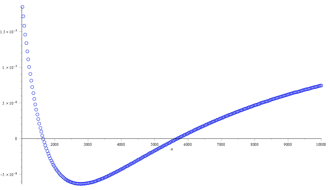
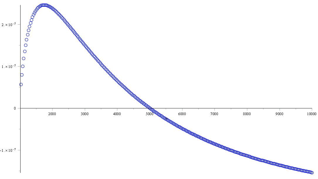
Figure 23: The Relative Error of $F_{7a}(n)$ when 1000 $\leqslant$ $n$ $\leqslant$ 10000, step 300

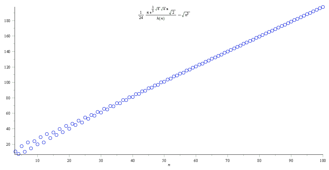
Figure 24: The Relative Error of $F_{7b}(n)$ when 1000 $\leqslant$ $n$ $\leqslant$ 10000, step 300

Figure 25: The graph of the data $\left(n,\,C_{8}(n)\right)$

3.5 Estimate $h(n)$ When $n\leqslant 100$

All the estimation function for $h(n)$ found now are with very good accuracy when $n$ is greater than 1000, but they are not so accurate when $n<50$, especially when $n<25$. Although $I^{\prime}_{\mathrm{g1}}(n)$ and $I^{\prime}_{\mathrm{g2}}(n)$ are better than others, the relative error are still greater than $1\permil$ when $n<40$.

Table 14: The relative error of $I_{\mathrm{g0}}(n)$ to $h(n)$ when $n\leqslant 100$.

Table 15: The relative error of $I^{\prime}_{\mathrm{g0}}(n)$ to $h(n)$ when $n\leqslant 100$.

When $n<40$, it is too difficult to fit $\frac{\pi\exp\left(\pi\sqrt{\frac{2}{3}}\sqrt{n}\right)}{12\sqrt{2}h(n)}-n^{3/2}$ by a simple smooth function with high accuracy, as shown on Figure 25 (on page 25). The figure of the points $\left(n,\ \frac{\pi\exp\left(\pi\sqrt{\frac{2}{3}}\sqrt{n}\right)}{12\sqrt{2}h(n)}-n^{3/2}\right)$ ( $n$ = 3, 4, $\cdots$, 100) is not so complicated (as shown on Figure 25). It seems that we can fit them by a simple piecewise function with 2 pieces, as the even points (where $n$ is even) lie roughly on a smooth curve, so do the odd points. If we try to fit them respectively, we will have the fitting function below:

$$C_{8}(x)=\begin{cases}1.942141112\times x-0.4796781366\times\sqrt{x}\\ \quad+8.291226268,\quad n=3,5,7,\cdots,99;&\\ 1.803056782\times x+2.356539877\times\sqrt{x}\\ \quad-6.043824511,\quad n=4,6,8\cdots,100.&\end{cases}$$ (34)

Hence we can calculate $h(n)$ ( $3\leqslant n\leqslant 100$) by

$$h(n)\sim I_{\mathrm{g0}}(n)=\frac{\pi\exp\left(\sqrt{\frac{2}{3}}\pi\sqrt{n}\right)}{12\sqrt{2}\left(n^{3/2}+C_{8}(n)\right)},\quad 3\leqslant n\leqslant 100.$$ (35)

Consider that $h(n)$ is an integer, we can take the round approximation of Equation (35),

$$I^{\prime}_{\mathrm{g0}}(n)=\left\lfloor\frac{\pi\exp\left(\sqrt{\frac{2}{3}}\pi\sqrt{n}\right)}{12\sqrt{2}\left(n^{3/2}+C_{8}(n)\right)}+\frac{1}{2}\right\rfloor,\quad 3\leqslant n\leqslant 100.$$ (36)

Here $n$ begins from 3, not 1 or 2, because $\frac{I^{\prime}_{\mathrm{g0}}(1)-h(1)}{h(1)}$ is meaningless since $h(1)=0$, and $I^{\prime}_{\mathrm{g0}}(2)$ differs from $h(2)$ a lot. Besides, the value of $h(1)$ and $h(2)$ are clear by definition, so there is no need to use a complicated formula to estimate them.

The relative error of $I_{\mathrm{g0}}(n)$ (or $I^{\prime}_{\mathrm{g0}}(n)$) to $h(n)$ are shown on Table 15 (or Table 15) on page 15. Compared them with Table 11 on page 11, we will find that when $n\geqslant 80$, $I^{\prime}_{\mathrm{g2}}(n)$ is more accurate than $I^{\prime}_{\mathrm{g0}}(n)$; when $n<80$, $I^{\prime}_{\mathrm{g0}}(n)$ is better.

4 Conclusion

We have presented a recursion formula and several practical estimation formulae with high accuracy to calculated the number $h(n)$ of conjugate classes of derangements of order $n$, or the number of isotopy classes of $2\times n$ Latin rectangles.

If we want to obtain the accurate value of $h(n)$, we can use the recursion formula (10) and write a program based on it, while sometimes we need to know the estimation value in a program for technique reason especially when we use a general programming language.

If we want to obtain the approximation value of $h(n)$ with high accuracy, we can use the formulae (31), (36), (29), etc.

When $2\leqslant n\leqslant 80$, we can use $I^{\prime}_{\mathrm{g0}}(n)$ (Equation (36)) , with a relative error less than 0.11% (while $32\leqslant n\leqslant 80$) or mainly 0 with very few exceptions (while $2\leqslant n\leqslant 31$); when $n>80$, we can use $I^{\prime}_{\mathrm{g2}}(n)$ (Equation (31)).

When $n\geqslant 100$, formulae $I^{\prime}_{\mathrm{ga}}(n)$ (Equation (27)), $I^{\prime}_{\mathrm{g1}}(n)$ (Equation (29)), $F_{7a}(n)$ (Equation (32)) and $F_{7b}(n)$ (Equation (33)) are also very accurate although they are not as good as Equations (31).

With the asymptotic formula (18) described in [30], we can obtain some estimation formulae with high accuracy for some other types of restricted partition numbers by the methods mentioned in this paper or in [1].

Data Availability

The figures and tables used to support this study are included within the article. The other data used to support this study are obtained from a program made by the first author.

Conflicts of Interest

The authors declare that there are no conflicts of interest regarding the publication of this paper.

References

[1]
W.-W. Li, “Estimation of the Partition Number: After Hardy and Ramanujan,”
ArXiv e-prints, Dec. 2016.
arXiv:1612.05526 [math.NT].
[2]
M. Hall, Jr., “A survey of combinatorial analysis,” in Some aspects
of analysis and probability (I. Kaplansky and etc, eds.), vol. IV of Surveys in applied mathematics, pp. 35 – 104, John Wiley and Sons, Inc.
[New York] and Chapman and Hall, Limited [London], 1958.
[3]
E. W. Weisstein, ““Partition Function P." From MathWorld – A Wolfram Web
Resource.” Internet: http://mathworld.wolfram.com/PartitionFunctionP.html
(accessed September 20, 2015), 1999-2015.
[4]
N. J. A. Sloane, “ A000041, number of partitions of (the partition
numbers). (Formerly M0663 N0244) , in “The On-Line Encyclopedia of Integer
Sequences (OEIS ®)".” Internet: http://oeis.org/A000041 (accessed
September 20, 2015).
[5]
Anonymous, ““Bibliography on Partitions" in “Mathematical BBS".”
Internet:
http://felix.unife.it/Root/d-Mathematics/d-Number-theory/b-Partitions
(accessed September 12, 2016), December 2007.
[6]
M. Newman, “Weighted restricted partitions,” Acta Arithmetica,
vol. 5, no. 4, pp. 371 – 380, 1959.
[7]
D. B. Lahiri, “Some restricted partition functions: Congruences modulo 3,”
Pacific Journal of Mathematics, vol. 28, no. 3, pp. 575 – 581, 1969.
Subjects: Primary: 10.48, MR0241377, Zentralblatt MATH identifier:
0172.05602.
[8]
D. B. Lahiri, “Some restricted partition functions: Congruences modulo 5,”
Journal of the Australian Mathematical Society, vol. 9,
pp. 424 – 432, May 1969.
[9]
D. B. Lahiri, “Some restricted partition functions: Congruences modulo 7,”
Transactions of the American Mathematical Society, vol. 140,
pp. 475 – 484, Jun. 1969.
Subjects: Primary 10.48, MR 0242784 (39 #4111).
[10]
R. Jakimczuk, “Restricted Partitions: Elementary Methods,” International Journal of Contemporary Mathematical Sciences, vol. 4, no. 2,
pp. 93 – 103, 2009.
[11]
B. Kronholm, “A result on Ramanujan-like congruence properties of the
restricted partition function p(n,m) across both variables,” INTEGERS:
The Electronic Journal of Combinatorial Number Theory, vol. 12, p. A63,
November 2012.
[12]
A. Folsom, Z. A. Kent, and K. Ono, “-adic properties of the partition
function,” Advances in Mathematics, vol. 229, pp. 1586 – 1609,
February 2012.
[13]
E. Belmont, H. Lee, A. Musat, and S. Trebat-Leder, “-adic properties of the
partition function,” Monatshefte für Mathematik, vol. 173,
pp. 1 – 34, January 2014.
[14]
K. Thanigasalam, “Congruence Properties of Certain Restricted Partitions,”
Mathematics Magazine, vol. 47, pp. 154 – 156, May 1974.
[15]
D. R. Hickerson, “A note on congruence properties of certain restricted
partitions,” Mathematics Magazine, vol. 48, p. 102, Mar. 1975.
[16]
M. Culek and A. Knecht, “Congruences of Restricted Partition Functions.”
Internet: http://citeseerx.ist.psu.edu/viewdoc/download?doi=
10.1.1.509.2649&rep=rep1&type=pdf (accessed October 02, 2015), 2002.
[17]
B. Kronholm, “On Congruence Properties of p(n, m),” Proceedings of the
American Mathematical Society, vol. 133, pp. 2891 – 2895, Oct. 2005.
[18]
B. Kronholm, “On Congruence Properties of Consecutive Values of ,”
INTEGERS: The Electronic Journal of Combinatorial Number Theory,
vol. 7, Mar. 2007.
#A16.
[19]
B. C. Berndt, “Ramanujan’s congruences for the partition function, modulo 5,
7, and 11,” International Journal of Number Theory, vol. 03,
pp. 349 – 354, September 2007.
[20]
G. E. Andrews and B. C. Berndt, “Ramanujan’s Unpublished Manuscript on the
Partition and Tau Functions,” in Ramanujan’s Lost Notebook: Part
III, pp. 89 – 180, Springer Science+Business Media New York, 2012.
[21]
B. Kronholm, “Generalized congruence properties of the restricted partition
function ,” The Ramanujan Journal, vol. 30, pp. 425 – 436,
April 2013.
[22]
N. J. A. Sloane, ““Restricted partitions" in OEIS wiki.” Internet:
http://oeis.org/wiki/Restricted_partitions (accessed September 20, 2015),
December 2011.
[23]
D. M. Bressoud, “Integer Partitions: Restricted Number and Part Size,” in
NIST Digital Library of Mathematical Functions (DLMF) (F. W. J.
Olver, D. W. Lozier, and R. F. Boisvert, eds.), August 2015.
Online companion to [25].
[24]
F. W. J. Olver, D. W. Lozier, and R. F. Boisvert, “Integer Partitions: Other
Restrictions,” in NIST Digital Library of Mathematical Functions
(DLMF) (F. W. J. Olver, D. W. Lozier, and R. F. Boisvert, eds.), National
Institute of Standards and Technology (NIST), August 2015.
Online companion to [25].
[25]
F. W. J. Olver, D. W. Lozier, and R. F. Boisvert, eds., NIST Handbook of
Mathematical Functions.
New York, NY: Cambridge University Press, May 2010.
Print companion to [24].
[26]
A. Greenbaum and T. P. Chartier, Numerical Methods: Design, Analysis, and
Computer Implementation of Algorithms.
New Jersey, NJ: Princeton University Press, Apr 2012.
[27]
D. Kincaid and W. Cheney, Numerical Analysis: Mathematics of Scientific
Computing, Third Edition, vol. 2 of Pure and Applied Undergraduate
Texts.
American Mathematical Society, 2002.
[28]
W. Lichten, Data and Error Analysis.
Prentice Hall, Oct 1998.
[29]
A. E. Ingham, “A Tauberian Theorem for Partitions,” Annals of
Mathematics, Second Series, vol. 42, pp. 1075 – 1090, Dec. 1941.
[30]
D. M. Kane, “An elementary derivation of the asymptotics of partition
functions,” The Ramanujan Journal, vol. 11, pp. 49 – 66,
February 2006.
[31]
G. H. Hardy and S. R. Ramanujan, “Asymptotic Formulae in Combinatory
Analysis,” Proceedings of the London Mathematical Society, s2,
vol. XVII, pp. 75 – 115, January 1918.
[32]
P. Erdős, “The Evaluation of the Constant in the Formula for the Number
of Partitions of ,” Annals of Mathematics. Second Series, vol. 43,
pp. 437 – 450, July 1942.
[33]
D. J. Newman, “The evaluation of the constant in the formula for the number of
partitions of ,” American Journal of Mathematics, vol. 73,
pp. 599 – 601, July 1951.
[34]
D. J. Newman, “A simplified proof of the partition formula,” The
Michigan Mathematical Journal, vol. 9, pp. 283 – 287, Jan. 1962.
MR0142529, ZMI 0105.26701.
[35]
T. M. Apostol, “Functions of Number Theory, Additive Number Theory:
Unrestricted Partitions,” in NIST Digital Library of Mathematical
Functions (DLMF) (F. W. J. Olver, D. W. Lozier, and R. F. Boisvert, eds.),
August 2015.
http://dlmf.nist.gov/27.14, Release 1.0.10 of 2015-08-07, (accessed
November 12, 2015).