Optimal-transport-based mesh adaptivity on the plane and sphere using finite elements

Abstract

In moving mesh methods, the underlying mesh is dynamically adapted without changing the connectivity of the mesh. We specifically consider the generation of meshes which are adapted to a scalar monitor function through equidistribution. Together with an optimal transport condition, this leads to a Monge–Ampère equation for a scalar mesh potential.

We adapt an existing finite element scheme for the standard Monge–Ampère equation to this mesh generation problem; this is a mixed finite element scheme, in which an extra discrete variable is introduced to represent the Hessian matrix of second derivatives. The problem we consider has additional nonlinearities over the basic Monge–Ampère equation due to the implicit dependence of the monitor function on the resulting mesh. We also derive an equivalent Monge–Ampère-like equation for generating meshes on the sphere. The finite element scheme is extended to the sphere, and we provide numerical examples. All numerical experiments are performed using the open-source finite element framework Firedrake.

Keywords: Monge–Ampère equation, mesh adaptivity, finite element, optimal transport

1 Introduction

1.1 Overview

This paper describes a robust, general-purpose algorithm for generating adaptive meshes. These can then be coupled to the computational solution of time-dependent partial differential equations. The algorithm is based on the finite element solution of a nonlinear partial differential equation of Monge–Ampère type, and can be used to generate meshes both on the plane and on the sphere. The underlying theory behind this procedure is derived from the concept of optimal transport. This guarantees the existence of well-behaved meshes which are immune to mesh tangling. The use of a quasi-Newton method to solve the resulting nonlinear system produces an algorithm that does not need tunable parameters to be effective for a wide variety of examples. We demonstrate the effectiveness of this method on a series of examples on both the plane and on the sphere. An example of such a mesh on the sphere is shown on the front page, and is discussed in more detail in section 5.

1.2 Motivation

The evolution of many physical systems can be expressed, to a close approximation, using partial differential equations. In many interesting cases, the solutions of these equations will develop structures at small scales, even if these scales were not present in the initial conditions. Such small-scale phenomena often have an important role in the future evolution of the system – examples include shocks in compressible flow problems, or interfaces in chemical reactions. We are particularly motivated by the area of weather prediction and climate simulation. A core task is the numerical solution of partial differential equations (variants of the Navier-Stokes equations) that model the evolution of the Earth’s atmosphere. Current state-of-the-art models have resolutions of approximately 10km for global forecasts. There will always be physical processes occurring at smaller length scales than can be resolved in such a model. However, it may be advantageous to vary the resolution dynamically. This could be used to better resolve features such as weather fronts and cyclones, which are meteorologically important and can result in severe weather leading to economic damage and loss of life.

Obtaining a numerical approximation to the solution of such problems usually involves formulating a discrete problem on a mesh. Typically, a uniform-resolution mesh is used. However, if the mesh cannot adequately resolve the small scale features, this process may lead to poor-quality results. In such cases, it may be necessary to use some form of dynamic mesh adaptivity to resolve evolving small scale features and other aspects of the solution. A common approach is to use a form of local mesh refinement ($h$-adaptivity) in which mesh points are added to regions where greater resolution is required. An alternative form of adaptivity is a mesh relocation strategy ($r$-adaptivity), in which mesh vertices are moved around without changing the connectivity of the mesh. This is done to increase the density of cells in regions where it is necessary to represent small scales.

$r$-adaptivity has certain attractive features: as mesh points are not created or destroyed, data structures do not need to be modified in-place and complicated load-balancing is not necessary. Furthermore, it avoids sharp changes in resolution, which can result in spurious wave propagation behaviour. A review of a number of different $r$-adaptive methods is given in Huang and Russell (2011). The simplest case of $r$-adaptivity involves the redistribution of a one-dimensional mesh. This has been implemented in several software libraries, such as the bifurcation package AUTO, and the procedure is currently used in operational weather forecasting within the data assimilation stage (Piccolo and Cullen, 2011, 2012). While $r$-adaptivity is not yet used in other areas of operational weather forecasting, it has been considered for geophysical problems in a research environment. Examples include Dietachmayer and Droegemeier (1992); Prusa and Smolarkiewicz (2003); Smolarkiewicz and Prusa (2005); Kühnlein et al. (2012); Budd et al. (2013).

For two- or three-dimensional problems, there is considerable freedom when choosing a relocation strategy. There has been a growing interest in optimally-transported $r$-adapted meshes (Budd and Williams, 2006; Delzanno et al., 2008; Budd and Williams, 2009; Delzanno and Finn, 2010; Chacón et al., 2011; Sulman et al., 2011; Budd et al., 2013; Browne et al., 2014; Budd et al., 2015; Weller et al., 2016; Browne et al., 2016). These methods minimise a deformation functional, subject to equidistributing a prescribed scalar monitor function which controls the local density of mesh points. The appropriate mesh can be derived from a scalar mesh potential which satisfies a Monge–Ampère equation. The solution of such an equation then becomes an important part of the strategy for relocating the mesh points.

Numerical methods for the Monge–Ampère equation go back to at least Oliker and Prussner (1989), which uses a geometric approach. A range of numerical schemes are present in the literature. Finite difference schemes include Loeper and Rapetti (2005); Benamou et al. (2010); Froese and Oberman (2011a, b); Benamou et al. (2014); several of these provably converge to viscosity solutions of the Monge–Ampère equation. Finite element schemes include Dean and Glowinski (2006a, b); Feng and Neilan (2009); Lakkis and Pryer (2013); Neilan (2014); Awanou (2015), which all introduce an extra discrete variable to represent the Hessian matrix of second derivatives, and Brenner et al. (2011); Brenner and Neilan (2012), which use interior penalty methods.

In the context of global weather prediction, there is an additional complication for mesh adaptivity: the underlying mesh is of the sphere, rather than a subset of the plane. The recent paper Weller et al. (2016) uses the exponential map to handle this, extending the Monge–Ampère-based approach on the plane. Weller et al. (2016) also presents a finite volume/finite difference approach for generating optimally-transported meshes on the sphere, and a comparison of the resulting meshes with those generated from an alternative approach, Lloyd’s algorithm. However, they did not discretise a Monge–Ampère equation on the sphere, but instead enforced a discrete equidistribution condition in each cell. The related paper Browne et al. (2016) then compares the nonlinear convergence of several different methods for solving the Monge–Ampère mesh generation problem on the plane, again in a finite volume context.

In this paper, we present a method for generating optimally-transported meshes on the plane and on the sphere from a given monitor function prescribing the local mesh density. This method uses a mixed finite element discretisation of the underlying Monge–Ampère (or Monge–Ampère-like) equation, which might be particularly useful if finite element methods are already being used to solve the model PDE for which mesh adaptivity is being provided. The finite element formulation also allows us to take advantage of the automated generation of Jacobians for Newton solvers. We give two variants of the method, which differ in how the nonlinear equation is solved. The first variant uses a relaxation method to generate progressively better approximations to the adapted mesh. The second variant uses a quasi-Newton method combined with a line search.

1.3 Summary of novel contributions

• We present a mixed finite element approach for the nonlinear Monge–Ampère-based mesh generation problem on the plane, based on Lakkis and Pryer (2013).

• We present a relaxation method for solving this nonlinear problem, an extension and modification of the scheme given in Awanou (2015), and a quasi-Newton method, which converges in far fewer nonlinear iterations and has no free parameter.

• We formulate a partial differential equation for the equivalent mesh-generation problem on the sphere. We present a nonlinear mixed finite element discretisation for this, and give relaxation and quasi-Newton approaches for solving this nonlinear problem.

1.4 Outline

The remainder of this paper is structured as follows. In section 2, we present background material. In particular, we show how optimally-transported meshes on the plane can be generated through the solution of a Monge–Ampère equation, and we present mixed finite element schemes from the existing literature for solving the basic Monge–Ampère equation. In section 3, we extend these finite element schemes to the mesh generation problem on the plane. In section 4, we present an equivalent approach for mesh generation on the sphere, based on an equation of Monge–Ampère type that we derive from an optimal transport problem. In section 5, we give a number of examples of meshes generated using these methods with analytically-prescribed monitor functions. We also give an example of a mesh adapted to the result of a numerical simulation. We consider examples of meshes on both the plane and the sphere, and comment on the convergence of the methods. We also discuss the nature of the resulting meshes. Finally, in section 6, we draw conclusions and discuss further work.

2 Preliminaries

2.1 Notation

We consider a ‘computational’ domain, $\Omega_{C}$, in which there is a fixed computational mesh, $\tau_{C}$, and a ‘physical’ domain, $\Omega_{P}$, with a target physical mesh, $\tau_{P}$, which should be adapted for simulating some physical system of interest. We will always assume that $\Omega_{C}$ and $\Omega_{P}$ represent the same mathematical domain: $\Omega_{C}=\Omega_{P}=\Omega$. For example, $\Omega$ may be the unit square $[0,1]^{2}$, the periodic unit square $\mathbb{R}^{2}/\mathbb{Z}^{2}$, or the surface of the sphere $S^{2}$. We denote positions in $\Omega_{C}$ by $\vec{\xi}$, and positions in $\Omega_{P}$ by $\vec{x}$.

The physical mesh $\tau_{P}$ will be the image of the computational mesh $\tau_{C}$ under the action of a suitably-smooth map $\vec{x}(\vec{\xi})$ from $\Omega_{C}$ to $\Omega_{P}$. Therefore, our aim is to find this map, or, rather, a discrete representation of it. The meshes $\tau_{C}$ and $\tau_{P}$ will have the same topology (connectivity) but different geometry. $\tau_{C}$ is typically uniform (or quasi-uniform), while the density of the mesh $\tau_{P}$ is controlled by a positive scalar monitor function, which we label $m$.

2.2 Optimally-transported meshes in the plane

2.2.1 Equidistribution

We wish to find the map

$$\vec{x}(\vec{\xi})\vcentcolon\Omega_{C}\to\Omega_{P}$$ (2.1)

such that the monitor function $m(\vec{x})$ is equidistributed. Letting $\theta$ be a normalisation constant, the equidistribution condition is precisely

$$m(\vec{x})\det J=\theta,$$ (2.2)

where $J$ represents the Jacobian of the map $\vec{x}(\vec{\xi})$:

$$J_{ij}=\frac{\partial x_{i}}{\partial\xi_{j}}.$$ (2.3)

It is clear that this problem is not well-posed in more than one dimension, as the desired map is far from unique. Intuitively, phrased in terms of meshes, eq. 2.2 sets the local cell area, but does not control the skewness or orientation of the cell. Accordingly, many different additional constraints/regularisations have been proposed for $r$-adaptive methods in order to generate a unique map. The following subsection describes a notable example of such a constraint.

2.2.2 Optimal transport maps and the Monge–Ampère equation

Using ideas from optimal transport (see Budd and Williams (2009) for a more detailed overview), the problem can be made well-posed at the continuous level by seeking the map closest to the identity (i.e., the mesh $\tau_{P}$ with minimal displacement from $\tau_{C}$) over all possible maps which equidistribute the monitor function. From classical results in optimal transport theory (Brenier, 1991), this problem has a unique solution, and (in the plane) the deformation of the resulting map can be expressed as the gradient of a scalar potential $\phi$:

$$\vec{x}(\vec{\xi})=\vec{\xi}+\nabla_{\vec{\xi}}\phi(\vec{\xi}),$$ (2.4)

where the quantity $\frac{1}{2}|\vec{\xi}|^{2}+\phi$ is automatically convex, guaranteeing that the map is injective . Substituting eq. 2.4 into eq. 2.2 then gives

$$m(\vec{x})\det(I+H(\phi))=\theta,$$ (2.5)

where $H(\phi)$ is the Hessian of $\phi$, with derivatives taken with respect to $\vec{\xi}$. In the plane, there are two sources of nonlinearity: first, the determinant includes a product of second derivatives ${(1+\phi_{\xi\xi})(1+\phi_{\eta\eta})-\phi_{\xi\eta}^{2}}$ (using the notation $\vec{\xi}=(\xi,\eta)$), hence the equation is of Monge–Ampère type; second, the monitor function $m$ is a function of $\vec{x}$, which depends on $\phi$ via eq. 2.4. We remark that the potential $\phi$ is only defined up to an additive constant.

More generally, we could have

$$m_{1}(\vec{x})\det(I+H(\phi))=m_{2}(\vec{\xi});$$ (2.6)

the case where $m_{2}$ is uniform reduces to eq. 2.5. However, we do not use this most general formulation in the remainder of the paper.

2.2.3 Boundary conditions

In our numerical experiments, we will only consider the doubly-periodic domain $\mathbb{R}^{2}/\mathbb{Z}^{2}$ and the sphere $S^{2}$. However, for general domains which have boundaries, it is natural to seek maps from $\Omega_{C}$ to $\Omega_{P}$ which also map the boundary of one domain to that of the other. In this case, eq. 2.5 must be equipped with boundary conditions. The Neumann boundary condition $\frac{\partial\phi}{\partial n}=0$ allows mesh vertices to move along the boundary (assuming a straight-line segment) but not away from it, per eq. 2.4. However, by equality of mixed partial derivatives, orthogonality is unnecessarily enforced at the boundary. For further discussion, see (for example) Delzanno et al. (2008).

We remark that, unlike in some other mesh adaptivity methods (such as the variational methods described in Huang and Russell (2011)), vertices on the boundary do not require special treatment in our method beyond the inclusion of boundary conditions for the resulting PDE. A limitation is that, using the Neumann condition, boundary vertices must remain on the same straight-line segment. Extending the approach to handle curved boundaries would require the inclusion of a complicated, nonlinear constraint. Benamou et al. (2014) presents a scheme that can handle the boundary-to-boundary mapping in the general case, where vertices are not restricted to the same straight-line segment.

2.3 Finite element methods for solving the Monge–Ampère equation

There are several finite element schemes in the literature for solving the Monge–Ampère equation, usually presented in the form

$$\det H(\phi)=f$$ (2.7)

inside a domain $\Omega$, with the Dirichlet boundary condition $\phi=g$ on $\partial\Omega$. There are certain convexity requirements on the domain and boundary data, but we will not discuss these here. The schemes that we use are adapted from Lakkis and Pryer (2013) and Awanou (2015).

Lakkis and Pryer (2013) presented a mixed finite element approach in which a tensor-valued discrete variable is introduced to represent the Hessian $H(\phi)$. We label this variable $\sigma$, which belongs to a finite element function space $\Sigma$. The scalar variable $\phi$ is in the function space $V$. The nonlinear discrete formulation of eq. 2.7 is then to find $\phi\in V,\sigma\in\Sigma$ satisfying

$$\langle v,\det\sigma\rangle =\langle v,f\rangle,\qquad \forall v\in\accentset{\circ}{V},$$ (2.8)

$$\langle\tau,\sigma\rangle+\langle\nabla\cdot\tau,\nabla\phi\rangle-\langle\langle\tau\cdot\vec{n},\nabla\phi\rangle\rangle =0,\qquad \forall\tau\in\Sigma,$$ (2.9)

together with the boundary condition $\phi=g$ on $\partial\Omega$, where $\accentset{\circ}{V}$ denotes the restriction of $V$ to functions vanishing on the boundary. Here, and in the rest of the paper, we use angle brackets to denote the $L^{2}$ inner product between scalars, vectors and tensors:

$$\langle a,b\rangle =\int_{\Omega}ab\,\mathrm{d}x,\qquad\qquad\qquad\langle\vec{a},\vec{b}\rangle=\int_{\Omega}\vec{a}\cdot\vec{b}\,\mathrm{d}x,$$ (2.10)

$$\langle\tau,\sigma\rangle =\int_{\Omega}\tau:\sigma\,\mathrm{d}x\equiv\int_{\Omega}\sum_{i}\sum_{j}\tau_{ij}\sigma_{ij}\,\mathrm{d}x.$$

Similarly, we use double angle brackets $\langle\langle\ \cdot\ \rangle\rangle$ for integrals over the boundary $\partial\Omega$.

Equation 2.8 is clearly a weak form of eq. 2.7 with the Hessian $H(\phi)$ replaced by the discrete Hessian $\sigma$. Equation 2.9 is derived by contracting

$$\sigma=H(\phi),$$ (2.11)

with the test-function $\tau$ and integrating by parts, which also produces a surface integral. Assuming a mesh of triangles, a suitable choice of function space is the standard $P_{n}$ space for $\phi$ and for each component of $\sigma$, with $n\geq 2$ – more concisely, $V=P_{n}$, $\Sigma=(P_{n})^{2\times 2}$.

Lakkis and Pryer (2013) suggests using Newton iterations on the nonlinear system eqs. 2.8 and 2.9, or a similar approach such as a fixed-point method. They observe that, in their numerical experiments, the convexity of $\phi$ (defined appropriately in Aguilera and Morin (2009)) is preserved at each Newton iteration. In the earlier but related paper Lakkis and Pryer (2011), the authors solve the resulting linear systems using the unpreconditioned GMRES algorithm.

Awanou (2015) proposes an alternative iterative method for obtaining a solution to the nonlinear system eqs. 2.8 and 2.9, effectively introducing an artificial time and using a relaxation method. Starting from some initial guess $(\phi^{0},\sigma^{0})$, one obtains a sequence of solutions $(\phi^{1},\sigma^{1}),(\phi^{2},\sigma^{2}),\ldots$ by considering the discrete linear problem

$$-\langle v,\operatorname{tr}\sigma^{k+1}\rangle =-\langle v,\operatorname{tr}\sigma^{k}\rangle+\Delta t\langle v,\det\sigma^{k}-f\rangle,$$ (2.12)

$$\langle\tau,\sigma^{k+1}\rangle+\langle\nabla\cdot\tau,\nabla\phi^{k+1}\rangle-\langle\langle\tau\cdot\vec{n},\nabla\phi^{k+1}\rangle\rangle =0,$$ (2.13)

with each $\phi^{k+1}=g$ on the boundary, for all $v\in\accentset{\circ}{V}$ and for all $\tau\in\Sigma$. Equation 2.12 is a discrete version of

$$-\frac{\operatorname{tr}H(\phi^{k+1})-\operatorname{tr}H(\phi^{k})}{\Delta t}=\det H(\phi^{k})-f,$$ (2.14)

which can be recognised as a forward Euler discretisation in (artificial) time of

$$-\frac{\partial}{\partial t}\nabla^{2}\phi=\det H(\phi)-f.$$ (2.15)

According to Awanou (2015), the sequence $(\phi^{k},\sigma^{k})_{k=0}^{\infty}$ converges to a solution of the nonlinear system eqs. 2.8 and 2.9 if $\Delta t$ is sufficiently small and if the initial guess $(\phi^{0},\sigma^{0})$ is sufficiently close. Unsurprisingly, if $\Delta t$ is too large, the sequence of solutions diverges wildly. The linear systems given by eqs. 2.12 and 2.13 can be solved using a standard preconditioned Krylov method on the monolithic system, or by using a Schur complement approach to eliminate $\sigma$.

As suggested in Lakkis and Pryer (2013), we can obtain a similar method by replacing the $-\langle v,\operatorname{tr}\sigma\rangle$ terms by $\langle\nabla v,\nabla\phi\rangle$. This is effectively an analytic Schur complement in which $\sigma^{k+1}$ has been eliminated for $\phi^{k+1}$. We then first solve

$$\langle\nabla v,\nabla\phi^{k+1}\rangle=\langle\nabla v,\nabla\phi^{k}\rangle+\Delta t\langle v,\det\sigma^{k}-f\rangle,\qquad\forall v\in\accentset{\circ}{V},$$ (2.16)

to obtain $\phi^{k+1}$, then recover $\sigma^{k+1}$ by solving

$$\langle\tau,\sigma^{k+1}\rangle=-\langle\nabla\cdot\tau,\nabla\phi^{k+1}\rangle+\langle\langle\tau\cdot\vec{n},\nabla\phi^{k+1}\rangle\rangle,\qquad\forall\tau\in\Sigma.$$ (2.17)

This is just a standard $H^{1}$ Poisson equation followed by a mass-matrix solve.

3 Mesh adaptivity using finite element methods

On the plane, recall from eq. 2.5 that we want to solve the Monge–Ampère equation

$$m(\vec{x})\det(I+H(\phi))=\theta,$$ (3.1)

where, as in eq. 2.4,

$$\vec{x}(\vec{\xi})=\vec{\xi}+\nabla_{\vec{\xi}}\phi(\vec{\xi}).$$ (3.2)

From here onwards, we will assume that we are working on the periodic plane. Then all surface integrals disappear, and $\accentset{\circ}{V}$ coincides with $V$. Adapting eqs. 2.8 and 2.9 to this problem gives the nonlinear equations

$$\langle v,m(\vec{x})\det(I+\sigma)\rangle =\langle v,\theta\rangle,\qquad \forall v\in V,$$ (3.3)

$$\langle\tau,\sigma\rangle+\langle\nabla\cdot\tau,\nabla\phi\rangle =0,\qquad \forall\tau\in\Sigma.$$ (3.4)

If the monitor function $m$ were a function of $\vec{\xi}$, it would be very straightforward to adapt the mixed finite element approaches presented in section 2.3. We could fully solve the PDE in the computational domain $\Omega_{C}$ to obtain $\phi$, then obtain the new mesh $\vec{x}(\vec{\xi})$ as a ‘postprocessing’ step via eq. 3.2. We remark that this last step is not trivial: $\phi\in P_{n}$, for some $n\geq 2$, and the derivative $\nabla\phi$ is (in general) discontinuous between cells. The position of the mesh vertex is then not well-defined. A solution is to $L^{2}$-project the pointwise-derivative into the continuous finite element space $[P_{1}]^{2}$, which is an appropriate function space for representing the coordinate field of the mesh. This gives

$$\vec{x}(\vec{\xi})=\vec{\xi}+\Pi_{[P_{1}]^{2}}\nabla\phi(\vec{\xi}).$$ (3.5)

It is possible that this step introduces spurious oscillations, but at present we have not found this to be a problem.

However, as $m$ is a function of $\vec{x}$, this additional nonlinearity has to be incorporated into the iterative schemes. Furthermore, the normalisation constant $\theta$ must be evaluated carefully to make the linear systems soluble. We present two different methods below, extending the mixed finite element approaches given in section 2.3.

3.1 Relaxation method

The first method we consider for solving the nonlinear equations eqs. 3.3 and 3.4 is an adaption of the modified Awanou method eqs. 2.16 and 2.17. Given a state $(\phi^{k},\sigma^{k})$, we obtain $(\phi^{k+1},\sigma^{k+1})$ as follows.

1. Use $\phi^{k}$ to evaluate the coordinates of the physical mesh $\tau_{P}$ via eq. 3.5.

2. Evaluate the monitor function $m(\vec{x})$ at the vertices of $\tau_{P}$; in our numerical examples, $m$ will be defined analytically. When performing integrals including $m$, we take $m$ to be in the finite element space $P_{1}$ on $\Omega_{C}$.

3. Evaluate the normalisation constant

   $$\theta^{k}\vcentcolon=\frac{\int_{\Omega_{C}}m\det(I+\sigma^{k})\,\mathrm{d}x}{\int_{\Omega_{C}}\,\mathrm{d}x}.$$ (3.6)

4. Obtain $\phi^{k+1}$ by solving

   $$\langle\nabla v,\nabla\phi^{k+1}\rangle=\langle\nabla v,\nabla\phi^{k}\rangle+\Delta t\langle v,m\det(I+\sigma^{k})-\theta^{k}\rangle,\qquad\forall v\in V.$$ (3.7)

   As remarked previously, this has a null space of constant $\phi$. We also see that the normalisation constant is required for consistency, by considering $v\equiv 1$.

5. Obtain $\sigma^{k+1}$ by solving

   $$\langle\tau,\sigma^{k+1}\rangle=-\langle\nabla\cdot\tau,\nabla\phi^{k+1}\rangle,\qquad\forall\tau\in\Sigma.$$ (3.8)

6. Evaluate termination condition (based on, e.g., a maximum number of iterations, or the $L^{2}$- or $l^{2}$-norm of some quantity being below a certain tolerance); stop if met.

3.1.1 Discussion

From the form of eq. 3.7, it is clear that this scheme will have linear convergence as, at each iteration, the change in solution is proportional to the current residual. We showed in eq. 2.15 that the relaxation method is effectively a discretisation of a parabolic equation, whose solution converges to the solution of the desired nonlinear problem as ‘time’ progresses. In a moving mesh context, this can be closely identified with the (one-dimensional) moving mesh equation MMPDE6 (see, for example, Budd et al. (2009)), and the parabolic Monge–Ampère approach in Budd and Williams (2006, 2009).

3.2 Quasi-Newton method

We consider a Newton-based approach as a second solution method. In a Newton-type method, we require algorithms to evaluate the nonlinear residual and the Jacobian at the current state. (The latter should not be confused with the Jacobian of the coordinate transformation eq. 2.3!) By implementing these algorithms separately, we can use a line search or similar method to increase the robustness of the nonlinear solver.

3.2.1 Residual evaluation

Given a state $(\phi^{k},\sigma^{k})$, we evaluate the nonlinear residual as follows.

1. Follow steps 1–3 of the relaxation method to obtain $m$ and $\theta^{k}$.

2. The residual is then

   $$\langle v,m\det(I+\sigma^{k})-\theta^{k}\rangle+\langle\tau,\sigma^{k}\rangle+\langle\nabla\cdot\tau,\nabla\phi^{k}\rangle,\qquad\forall v\in V,\tau\in\Sigma,$$ (3.9)

   which corresponds to writing eqs. 3.3 and 3.4 in the form “$F(\phi,\sigma)=0$”. As this is a mixed finite element problem, eq. 3.9 should be interpreted as two subvectors, where the $i$th component of the first subvector is eq. 3.9 with $v$ replaced by the $i$th basis function of $V$ and $\tau$ replaced by zero, and the $i$th component of the second subvector is eq. 3.9 with $v$ replaced by zero and $\tau$ replaced by the $i$th basis function of $\Sigma$.

3.2.2 Jacobian evaluation

Given a state $(\phi^{k},\sigma^{k})$, we evaluate the (approximate) Jacobian as follows.

1. Follow steps 1–3 of the relaxation method to obtain $m$ and $\theta^{k}$.

2. The approximate Jacobian is then a partial linearisation of eq. 3.9 about the state $(\phi^{k},\sigma^{k})$, represented by the bilinear form

   $$\langle v,m(\delta\sigma_{11}(1+\sigma^{k}_{22})+(1+\sigma^{k}_{11})\delta\sigma_{22}-\delta\sigma_{12}\sigma^{k}_{21}-\sigma^{k}_{12}\delta\sigma_{21})\rangle\\ +\langle\tau,\delta\sigma\rangle+\langle\nabla\cdot\tau,\nabla\delta\phi\rangle,\quad\forall v\in V,\tau\in\Sigma.$$ (3.10)

   As we have a mixed finite element problem, this should be interpreted as a $2\times 2$ block matrix, where the separate blocks correspond to terms involving $(v,\delta\phi)$, $(v,\delta\sigma)$, $(\tau,\delta\phi)$ and $(\tau,\delta\sigma)$. Note that the first of these blocks is empty. The Jacobian is, of course, formally singular, since $\delta\phi$ is only defined up to a constant.

3.2.3 Discussion

The Jacobian we have presented, eq. 3.10, is not a full linearisation of eq. 3.9 since we have neglected the term resulting from the dependence of $m$ on $\phi$. Experimentally, we find that including this first-order term often causes the nonlinear solver to produce an intermediate solution that doesn’t satisfy the convexity requirements of the Monge–Ampère equation (the corresponding mesh, via eq. 3.5, is tangled). The next linear solve is then ill-posed as the Jacobian is no longer positive definite.

As we remarked previously in section 2.3, Lakkis and Pryer (2013) noted that their solution remained convex when solving the basic Monge–Ampère problem with a Newton method; in that case, the full Jacobian does not have a first-order term. While neglecting the first-order term seems to aid us with respect to keeping the linear problems well-posed, we expect that the neglected term is truly “$\mathcal{O}(1)$” – it does not tend to zero as we approach the solution of the nonlinear problem – and so the convergence of the method will only be linear.

As an alternative, but related, solution procedure, we could consider the normalisation constant $\theta$ to be another unknown in the nonlinear system. The nonlinear problem would then be to find $(\phi,\sigma,\theta)\in V\times\Sigma\times\mathbb{R}$ such that

$$\langle v,m(\vec{x})\det(I+\sigma)\rangle-\langle v,\theta\rangle =0,\qquad \forall v\in V$$ (3.11)

$$\langle\tau,\sigma\rangle+\langle\nabla\cdot\tau,\nabla\phi\rangle =0,\qquad \forall\tau\in\Sigma$$ (3.12)

$$\langle\lambda,\phi\rangle =0,\qquad \forall\lambda\in\mathbb{R},$$ (3.13)

where $\mathbb{R}$ represents the space of globally-constant functions, i.e., real numbers. Furthermore, this formulation eliminates the null space of constant $\phi$, but at the cost of introducing a dense row and column into the Jacobian matrix.

4 Mesh adaptivity on the sphere

On the sphere $S^{2}$, we again seek to equidistribute a prescribed scalar monitor function over a mesh $\tau_{P}$ defined on the curved surface. As in Weller et al. (2016), we make this well-posed by seeking the mesh $\tau_{P}$ with minimal displacement from $\tau_{C}$, measured by squared geodesic distance along the sphere. We rely on the result from McCann (2001): for such optimally-transported meshes, there exists a unique scalar mesh potential $\phi$ such that $\vec{x}$ and $\vec{\xi}$ are related through the exponential map, denoted as

$$\vec{x}=\exp(\nabla\phi)\vec{\xi},$$ (4.1)

where $\nabla$ is the usual surface gradient with respect to $\vec{\xi}$. The function $\phi$ is automatically $c$-convex with respect to the squared-geodesic-distance cost function; this is a natural generalisation of the earlier results for the plane.

The exponential map is a map from the tangent plane $T_{\xi}$ at a point on the sphere, $\vec{\xi}$, to the sphere. Intuitively, it is defined as the result of moving a distance $|\nabla\phi|$ along a geodesic (for the sphere, great circle) starting at $\vec{\xi}$, initially travelling in the direction $\nabla\phi$. Indeed, this map is defined for arbitrary manifolds, and reduces to eq. 2.4 in the plane. For a sphere of radius $R$ centred at the origin, the exponential map can be written explicitly as

$$\exp(\nabla\phi)\vec{\xi}=\cos\left(\frac{|\nabla\phi|}{R}\right)\vec{\xi}+R\sin\left(\frac{|\nabla\phi|}{R}\right)\frac{\nabla\phi}{|\nabla\phi|},$$ (4.2)

a reduction of Rodrigues’ well-known rotation formula.

4.1 Formulation of a Monge–Ampère-like equation for obtaining the mesh potential on the sphere

Consider some small open set $U\subset S^{2}$ containing the point $\vec{\xi}\in S^{2}$. The set will be mapped to an image set $V$ under the action of the map eq. 4.1. Define $r_{\phi}(\vec{\xi})$ to be the limiting ratio of the area of $V$, $|V|$, to the area of $U$, $|U|$, in the limit $|U|\to 0$. On the plane, this was simply $\det J$, i.e., $\det(I+\nabla\nabla\phi(\vec{\xi}))$. However, the corresponding expression is more subtle for the sphere. We therefore derive an expression for the ratio of areas in this case, and hence a partial differential equation for obtaining the mesh potential $\phi$.

We formulate the problem using Cartesian coordinates with the sphere embedded in three-dimensional space centred at the origin; this avoids problems with the singularities of an intrinsic coordinate system. Recall eq. 2.2 for the plane: ${m(\vec{x})\det J=\theta}$, where $J=\nabla\vec{x}$. This cannot be used directly, as $J$ will be a $3\times 3$ matrix when using the embedded coordinates, but only has rank two, so the determinant is trivially zero. One possibility is to use the pseudo-determinant of $J$: the ratio of areas is the product of the two non-zero singular values of $J\vcentcolon=\nabla\exp(\nabla\phi)\vec{\xi}$.

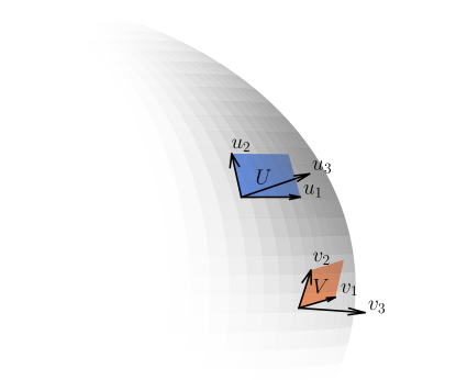
Figure 1: Diagram to aid the derivation in section 4.1. The area element $U$ is parametrised by $\vec{u}_{1}$ and $\vec{u}_{2}$, while $\vec{u}_{3}$ points radially outwards. This is mapped to the area element $V$, parametrised by $\vec{v}_{1}$ and $\vec{v}_{2}$, with $\vec{v}_{3}$ pointing radially outwards.

We instead produce an equivalent object with full rank . In fig. 1, consider the area element $U\subset\Omega_{C}$ to be parameterised by vectors $\vec{u}_{1}$, $\vec{u}_{2}$ which are tangent to $S^{2}$. The corresponding image area element $V\subset\Omega_{P}$ is parameterised by the image tangent vectors $\vec{v}_{1}$, $\vec{v}_{2}$. Define $\vec{k}_{C}$ to be the unit outwards normal vector at $\vec{\xi}$, and $\vec{k}_{P}$ to be the unit outwards normal vector at $\vec{x}$:

$$\vec{k}_{C}\vcentcolon=\vec{\xi}/R,\qquad\vec{k}_{P}\vcentcolon=\vec{x}/R.$$ (4.3)

In the infinitesimal limit, the area elements $U$ and $V$ can each be converted into volume elements of equal magnitude by extruding them radially outwards a distance 1 along $\vec{u}_{3}=\vec{k}_{C}$ and $\vec{v}_{3}=\vec{k}_{P}$, respectively. The volumes of these elements are given by $\det(\vec{u}_{1}\ \vec{u}_{2}\ \vec{u}_{3})$ and $\det(\vec{v}_{1}\ \vec{v}_{2}\ \vec{v}_{3})$. We claim that

$$(\vec{v}_{1}\ \vec{v}_{2}\ \vec{v}_{3})=\left((\nabla\exp(\nabla\phi)\vec{\xi})\cdot P_{\xi}+\vec{k}_{P}\otimes\vec{k}_{C}\right)(\vec{u}_{1}\ \vec{u}_{2}\ \vec{u}_{3}),$$ (4.4)

where $P_{\xi}\vcentcolon=I-\vec{k}_{C}\otimes\vec{k}_{C}$ is a projection matrix.

This can be shown as follows: by design, $P_{\xi}\vec{u}_{i}=\vec{u}_{i}$ for $i=1,2$, while $P_{\xi}\vec{u}_{3}=0$. The Jacobian of the exponential map, $\nabla\exp(\nabla\phi)\vec{\xi}$, maps tangent vectors $\vec{u}_{1},\vec{u}_{2}$ to tangent vectors $\vec{v}_{1},\vec{v}_{2}$, so $\left((\nabla\exp(\nabla\phi)\vec{\xi})\cdot P_{\xi}\right)(\vec{u}_{1}\ \vec{u}_{2}\ \vec{u}_{3})=(\vec{v}_{1}\ \vec{v}_{2}\ \vec{0})$. On the other hand, $\vec{k}_{C}\cdot\vec{u}_{i}=0$ for $i=1,2$, and $\vec{k}_{C}\cdot\vec{u}_{3}=1$, so $\left(\vec{k}_{P}\otimes\vec{k}_{C}\right)(\vec{u}_{1}\ \vec{u}_{2}\ \vec{u}_{3})=(\vec{0}\ \vec{0}\ \vec{k}_{P})=(\vec{0}\ \vec{0}\ \vec{v}_{3})$. Adding these together gives the claimed result. The volume ratio, and therefore area ratio, is then the determinant of the quantity in the large brackets in eq. 4.4. After replacing $\vec{k}_{C}$ and $\vec{k}_{P}$ by expressions involving $\vec{\xi}$ and $\phi$, this gives

$$r_{\phi}(\vec{\xi})=\det\left((\nabla\exp(\nabla\phi)\vec{\xi})\cdot P_{\xi}+\frac{\exp(\nabla\phi)\vec{\xi}}{R}\otimes\frac{\vec{\xi}}{R}\right).$$ (4.5)

The exponential map can then be replaced by the expression eq. 4.2, although for brevity we did not do this in eq. 4.5. The corresponding equation for mesh generation is then

$$m(\vec{x})\det\left((\nabla\exp(\nabla\phi)\vec{\xi})\cdot P_{\xi}+\frac{\exp(\nabla\phi)\vec{\xi}}{R}\otimes\frac{\vec{\xi}}{R}\right)=\theta.$$ (4.6)

Due to its construction, this equation will have similar numerical properties to the Monge–Ampère equation on the plane.

4.2 A numerical method for the equation of Monge–Ampère type on the sphere

We now present a numerical method for finding approximate solutions to eq. 4.6. We adapt the mixed finite element methods given in section 3 to this equation posed on $S^{2}$. Accordingly, we define the auxiliary variable as

$$\sigma=\nabla\exp(\nabla\phi)\vec{\xi}.$$ (4.7)

The nonlinear discrete equations are then

$$\left\langle v,m(\vec{x})\det\left(\sigma\cdot P_{\xi}+\frac{\exp(\nabla\phi)\vec{\xi}}{R}\otimes\frac{\vec{\xi}}{R}\right)\right\rangle =\langle v,\theta\rangle,\qquad \forall v\in V,$$ (4.8)

$$\langle\tau,\sigma\rangle+\langle\nabla\cdot\tau,\exp(\nabla\phi)\vec{\xi}\rangle =0,\qquad \forall\tau\in\Sigma.$$ (4.9)

This can be solved using a relaxation method, as in section 3.1, or with a quasi-Newton method, as in section 3.2. In the latter case, we make use of automatic differentiation techniques to avoid calculating the Jacobian manually. The only step that requires significant modification is obtaining the coordinates of the physical mesh $\tau_{P}$ from a given $\phi^{k}$. Assuming that the coordinate field of the sphere mesh is in the finite element space $[P_{n}]^{3}$ for some $n>1$, we now do this as follows:

1. Calculate the $L^{2}$-projection of the pointwise surface gradient of $\phi$ into $[P_{n}]^{3}$:

   $$\vec{w}=\Pi_{[P_{n}]^{3}}\nabla\phi(\vec{\xi}).$$ (4.10)

2. Ensure that $\vec{w}$ is strictly tangential to the sphere: at each mesh node, calculate

   $$\vec{w}^{\prime}=\vec{w}-\frac{\vec{w}\cdot\vec{\xi}}{R^{2}}\vec{\xi}.$$ (4.11)

3. Evaluate the coordinates of $\tau_{P}$ using eq. 4.2:

   $$\vec{x}=\cos\left(\frac{|\vec{w}^{\prime}|}{R}\right)\vec{\xi}+R\sin\left(\frac{|\vec{w}^{\prime}|}{R}\right)\frac{\vec{w}^{\prime}}{|\vec{w}^{\prime}|}.$$ (4.12)

5 Numerical results

In this section, we give several examples of meshes produced using the methods we described in section 3, using analytically-defined monitor functions. We comment on the convergence of the relaxation and quasi-Newton schemes for these examples, and we also give an example of a mesh adapted to the output of a quasi-geostrophic simulation. Finally, we verify that our method generates well-behaved meshes even at much higher mesh resolutions.

We implemented these numerical schemes using the finite element software Firedrake (Rathgeber et al., 2016). We make use of recently-developed functionality in Firedrake, including the use of quadrilateral meshes (Homolya and Ham, 2016; McRae et al., 2016; Homolya et al., 2017a), and the ability to solve PDEs on immersed manifolds (Rognes et al., 2013). The new form compiler TSFC (Homolya et al., 2017b) turns out to be particularly important due to its native support for higher-order coordinate fields, as we will see shortly, and its ability to do point evaluation. Our quasi-Newton implementation makes use of the automatic differentiation functionality of UFL (Alnæs et al., 2014), which is particularly helpful on the sphere, and the local assembly kernels are automatically optimised by COFFEE (Luporini et al., 2017). Finally, we use linear and nonlinear solvers from the PETSc library (Balay et al., 2016, 1997), via Firedrake and petsc4py (Dalcin et al., 2011).

5.1 Meshes on the periodic plane

We use the domain $[0,1]^{2}$ with doubly-periodic boundary conditions. In these examples, this is meshed as a 60 x 60 grid of squares. We use the finite element spaces $V=Q_{2}$, $\Sigma=(Q_{2})^{2\times 2}$ – this varies slightly from Lakkis and Pryer (2013) and Awanou (2015), which both used triangular meshes and hence used the $P_{n}$ family of finite element spaces.

We define some diagnostic measures of convergence in order to analyse the methods. Inspired by the PDE eq. 3.3, we expect the $l^{2}$-norm of the residual vector

$$\langle v,m\det(I+\sigma^{k})-\theta^{k}\rangle,\qquad\forall v\in V,$$ (5.1)

to tend to zero. We normalise this by the $l^{2}$-norm of $\langle v,\theta^{k}\rangle$. This diagnostic is related to the solution of the discrete nonlinear PDE, but the physical mesh $\tau_{P}$ only appears indirectly during the generation of $m$. We therefore introduce a second measure. Define

$$M_{i}\vcentcolon=\frac{\int_{e^{P}_{i}}m\,\mathrm{d}x}{\int_{e^{C}_{i}}\,\mathrm{d}x}$$ (5.2)

the integral of $m$ over the $i$th cell of $\tau_{P}$, normalised by the area of the corresponding cell of $\tau_{C}$. The second, “equidistribution”, measure is then the coefficient of variation of the $M_{i}$ – the standard deviation divided by the mean. Unlike in Weller et al. (2016), this quantity will not converge to zero (on a fixed mesh) in our method due to discretisation error. The quantity will approach zero on a sequence of refined meshes, however, and we investigate this further in section 5.4.

We use the same monitor function examples as used in Weller et al. (2016): a ‘ring’ monitor function

$$m(\vec{x})=1+10\operatorname{sech}^{2}(200(|\vec{x}-\vec{x_{c}}|^{2}-0.25^{2}))$$ (5.3)

and a ‘bell’ monitor function

$$m(\vec{x})=1+50\operatorname{sech}^{2}(100|\vec{x}-\vec{x_{c}}|^{2}),$$ (5.4)

where $\vec{x_{c}}$ denotes the centre of the feature. We take $\vec{x_{c}}$ to be the centre of the mesh, (0.5, 0.5), in our examples. The resulting meshes, which have mesh cells concentrated where the monitor function is large, are shown in fig. 2 (these were generated numerically with the relaxation scheme).

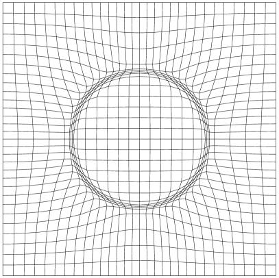
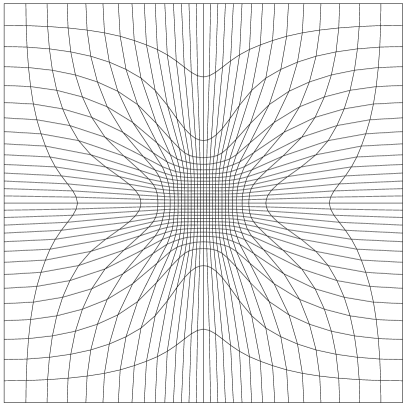
Figure 2: Meshes adapted to the ring monitor function eq. 5.3 and the bell monitor function eq. 5.4. The meshes are notably well-behaved in the transition regions between areas of low and high mesh concentration. For visualisation purposes, the above meshes are 30 x 30 rather than 60 x 60.

5.1.1 Relaxation method

Our implementation of the relaxation method differs very slightly from what was described in section 3.1: we evaluate diagnostics (and the termination condition) between steps 3 and 4. We terminate the method when the normalised $l^{2}$ residual is below $10^{-8}$. In practice, it is very unlikely that a mesh will need to be generated this accurately, but we want to illustrate that the scheme is convergent.

There is one free parameter in the relaxation method, namely the ‘step size’ $\Delta t$. This has to be chosen with some care. If it is too large then the iterations diverge and method is unstable. However, if it is too small then the number of iterations is unnecessarily large, wasting time. The optimal value is highly dependent on the monitor function $m$, and unfortunately we do not have a method for estimating it in advance. Empirically, we take $\Delta t$ as 0.1 for the ring monitor function, and 0.04 for the bell.

To solve the Poisson problem, and hence to obtain the iterate $\phi^{k+1}$, we use the CG method with GAMG, a geometric algebraic multigrid preconditioner. To obtain $\sigma^{k+1}$, we invert the mass matrix using ILU-preconditioned CG. The constant nullspace is handled by the Krylov solver.

The convergence properties of the relaxation method are shown in fig. 3. As can be expected from the form of the method, the convergence of the $l^{2}$-norm measure is linear. The equidistribution measure initially decreases at the same rate, but converges to some non-zero value. We see that the bell monitor function requires far more iterations (4.5x) than the ring monitor function to reach the same level of convergence, and that this is not simply due to the smaller step size.

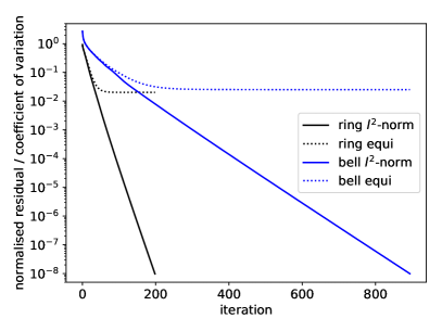
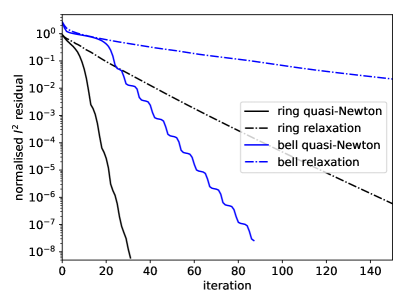
Figure 3: Left: convergence of diagnostic measures eqs. 5.1 and 5.2 when using the relaxation method, for the plane monitor functions eqs. 5.3 and 5.4. The residual converges to zero exponentially; the equidistribution measure initially decreases at the same rate but does not go to zero. Right: comparison of the convergence of the quasi-Newton and relaxation methods for these monitor functions. The quasi-Newton method also converges linearly, but in far fewer iterations than the relaxation method.

5.1.2 Quasi-Newton method

We have also implemented the scheme described in section 3.2. We use a line search method that minimises the $l^{2}$-norm of the residual at each nonlinear iteration, as described in Brune et al. (2015), terminating when the residual has decreased to $10^{-8}$ of its initial size. In our numerical examples, we do 5 inner iterations to determine the step-length $\lambda$ at each nonlinear iteration; in practice 1 or 2 such iterations is likely to be sufficient. We remark that, since our approximate Jacobian omits an “$\mathcal{O}(1)$ term”, the step length will not tend to 1 as we converge to the solution.

We use the GMRES algorithm to solve the linear systems, preconditioned using a block Gauss-Seidel algorithm, as defined in Brown et al. (2012). We use a custom preconditioning matrix, in which the diagonal blocks are replaced by those from the Riesz map operator

$$\langle v,\delta\phi\rangle_{H^{1}}+\langle\tau,\delta\sigma\rangle_{L^{2}};$$ (5.5)

this is sufficient to give asymptotically mesh-independent convergence . More details on the inspiration for such preconditioners can be found in Mardal and Winther (2011). On the $\delta\phi$ block, we precondition with GAMG, which uses the default Chebyshev-accelerated ILU smoothing; on the $\delta\sigma$ block we precondition with ILU. We again have the Krylov solver project out the constant nullspace, and the overall linear system is solved to the default relative tolerance of $10^{-5}$.

The convergence of the quasi-Newton method is shown in fig. 3. We see that convergence is reached in far fewer iterations than for the relaxation method. However, the convergence is still linear due to the use of an approximate Jacobian. The convergence behaviour is notably ‘wavy’, particularly in the bell case. This is possibly a side-effect of the line search technique, although we remark that similar behaviour is seen in Browne et al. (2016). Using this method on a range of different problem sizes (not shown here), we observe that the nonlinear convergence is essentially mesh-independent. More details are given in section 5.3.

5.1.3 Adaptation of a mesh to interpolated simulation data

As a more realistic example, we consider a mesh adapted to the output of a numerical simulation performed on a higher-resolution fixed mesh. Compared to the previous examples, the evaluation of an analytically-prescribed monitor function at arbitrary points in space is replaced by the evaluation of a finite element field that lives on a separate grid using interpolation.

We use the quasi-geostrophic equations. The velocity, $\vec{u}$, is defined to be the 2D curl of a scalar streamfunction, $\psi$:

$$\vec{u}=\nabla^{\perp}\psi.$$ (5.6)

The potential vorticity, $q$, is linked to the streamfunction by

$$\nabla^{2}\psi-\operatorname{Fr}\psi=q,$$ (5.7)

where $\operatorname{Fr}$ is the Froude number, a physical quantity that we here set to 1. The system then evolves according to

$$\frac{\partial q}{\partial t}+\nabla\cdot(q\vec{u})=0.$$ (5.8)

We use SSPRK3 timestepping (Shu and Osher, 1988). $q$ is represented using discontinuous, piecewise-linear elements; we use the standard upwind-DG formulation for the evolution equation eq. 5.8. $\psi$ is represented using continuous, piecewise linear elements; within each Runge–Kutta stage, we invert eq. 5.7 to obtain $\psi$ from $q$. The discretisation is from Bernsen et al. (2006), and the code is based on a tutorial available on the Firedrake website.

For the numerical simulation, we use the periodic unit square $[0,1]^{2}$. This is uniformly divided into a 100 x 100 grid of squares, and each square is subdivided into two triangles. We initialise $q$ as a continuous field of grid-scale noise, with each entry drawn uniformly from $[-1,1]$. Coherent vortices form over time. The $q$ field at $T=500$ is shown on the left in fig. 4. Although values of $q$ are analytically preserved, per eq. 5.8 (since the velocity field is divergence-free), due to discretisation error $q$ only takes values in $[-0.4,0.38]$ by this point in the numerical simulation.

To create a monitor function, we project this $q$ into a continuous space, which helps greatly with numerical robustness. We use the monitor function $m=q^{2}$, with the condition that this must be at least 0.005; this is to prevent the mesh density going to zero. As before, we start with a 60 x 60 grid of quadrilaterals, and adapt this to the monitor function using the quasi-Newton method. The resulting mesh is shown on the right in fig. 4.

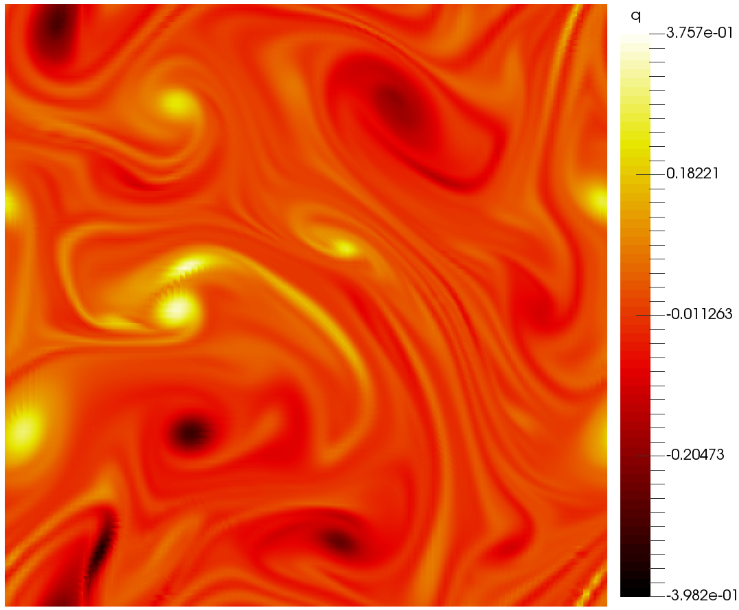
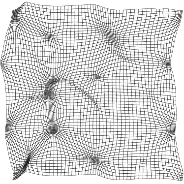
Figure 4: Left: potential vorticity field generated by quasi-geostrophic simulation on a doubly-periodic domain, as discussed in section 5.1.3. Right: optimally-transported mesh adapted to a monitor function based on this field.

5.2 Meshes on the sphere

In these examples, we set $\Omega_{C}$ and $\Omega_{P}$ to be the surface of a unit sphere. There are many ways to mesh a sphere: in weather forecasting, a latitude–longitude mesh is common, although we do not use this here. We firstly take $\tau_{C}$ to be a cubed-sphere mesh comprised of 6 x $16^{2}$ quadrilaterals on the surface of the sphere. In the later example, we use an icosahedral mesh of 20 x $16^{2}$ triangles.

We present results for both bilinear (lowest-order) and biquadratic representations of the sphere, where this refers to the polynomial order of the map from a “reference element” (in the context of finite element calculations) to each mesh cell. The biquadratic representation is more faithful than the bilinear representation, but formally there is no additional smoothness: both are only $C^{0}$. We continue to use biquadratic ($Q_{2}$) finite elements to represent $\phi$ and $\sigma$, independent of the representation of the mesh. The precise finite element spaces $V$ and $\Sigma$ are only defined implicitly: we use $Q_{2}$ basis functions on the reference cell, but we never explicitly construct the corresponding basis functions on the surface of the sphere. Rather, all calculations are performed in the reference element, and we only need to evaluate (at appropriate quadrature points) the Jacobian of the coordinate mapping from the reference element. Further details on the implementation of finite element problems on manifolds can be found in, for example, Rognes et al. (2013).

We use the same diagnostic measures as on the plane, adapted appropriately to the equation we solve on the sphere. We add a third diagnostic measure: for certain choices of monitor function (i.e., functions which are symmetric about some axis), the continuous problem eq. 4.6 reduces to a one-dimensional equation. This can be solved numerically to obtain the desired map $\vec{x}^{\>e}(\vec{\xi})$ to an arbitrary degree of accuracy (details are given in appendix A). We can then compute the difference between the ‘exact’ mesh coordinates, produced in this way, and the coordinates produced via the numerical solution of eq. 4.6. The diagnostic measure is then the root mean square of the vertex deviation,

$$\|\vec{x}-\vec{x}^{\>e}\|\vcentcolon=\sqrt{\frac{\sum_{i}\|\vec{x}_{i}-\vec{x}_{i}^{\>e}\|^{2}}{N}},$$ (5.9)

where $\|\cdot\|$ represents the geodesic distance. Again, due to discretisation errors, this will not converge to zero on a fixed mesh.

We use the (axisymmetric) monitor function

$$m(\vec{x})=\sqrt{\frac{1-\gamma}{2}\left(\tanh\frac{\beta-\|\vec{x}-\vec{x_{c}}\|}{\alpha}+1\right)+\gamma},$$ (5.10)

which is based on a mesh density function given in Ringler et al. (2011) . This monitor function produces an ‘inner region’, in which the monitor function approaches 1, and an ‘outer region’, in which the monitor function approaches $\sqrt{\gamma}$. Writing $\gamma=\kappa^{4}$, the ratio of cell edge lengths between the two regions is $\kappa$. The inner region has radius $\beta$, centred on $\vec{x_{c}}$, and the transition occurs over a lengthscale $\alpha$.

As in Ringler et al. (2011) and Weller et al. (2016), we take $\alpha=\pi/20$, $\beta=\pi/6$, and $\vec{x_{c}}$’s latitude to be 30 degrees North. We consider $\gamma=(1/2)^{4},(1/4)^{4},(1/8)^{4},(1/16)^{4}$. The resulting meshes are referred to as X2, X4, X8 and X16 meshes, where the number refers to the ratio of edge lengths between the inner and outer regions. The X2 (most gentle) and X16 (most extreme) cubed-sphere meshes are shown in figs. 5 and 6; these were generated numerically using the relaxation method with a biquadratic cell representation.

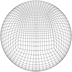
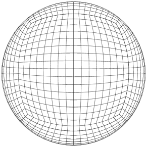
Figure 5: Front and rear of the cubed-sphere X2 mesh adapted to the monitor function given by eq. 5.10 with $\gamma=(1/2)^{4}$.

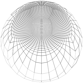
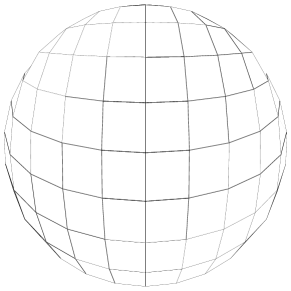
Figure 6: Front and rear of the cubed-sphere X16 mesh adapted to the monitor function given by eq. 5.10 with $\gamma=(1/16)^{4}$.

In our second example, we take $\tau_{C}$ to be a regular icosahedral mesh. We use the (non-axisymmetric) monitor function

$$m(\vec{x})=1+\alpha\operatorname{sech}^{2}(\beta(\|\vec{x}-\vec{x_{1}}\|^{2}-(\pi/2)^{2}))+\alpha\operatorname{sech}^{2}(\beta(\|\vec{x}-\vec{x_{2}}\|^{2}-(\pi/2)^{2})),$$ (5.11)

with $\alpha=10$ and $\beta=5$. The ‘poles’ $\vec{x_{1}}$ and $\vec{x_{2}}$ are chosen such that the bands cross at a $60^{\circ}$/$120^{\circ}$ angle: $\vec{x_{1,2}}=(\pm\frac{\sqrt{3}}{2},0,\frac{1}{2})$. On this triangular mesh, we use a quadratic representation of the mesh cells, and we use quadratic finite elements to represent $\phi$ and $\sigma$. The resulting mesh, obtained numerically via the quasi-Newton method, is shown in fig. 7. We do not show the convergence of our methods for this monitor function as the behaviour is qualitatively identical to the convergence of the first example.

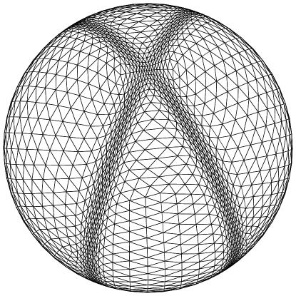
Figure 7: An icosahedral mesh adapted to the monitor function given by eq. 5.11. The mesh is well-aligned to the two bands, and is very regular at the intersection and away from the bands.

5.2.1 Relaxation method

We implemented a relaxation method for the sphere in the same way as for the plane. To avoid significant over/underintegration, we use a quadrature rule capable of integrating expressions of degree 8 exactly. All other options, including the linear solver choices and the termination criteria, are identical. We only analyse the X2 and X16 problems, as these are the least and most extreme, respectively. We take the step size parameter $\Delta t$ to be 2.0 in both cases.

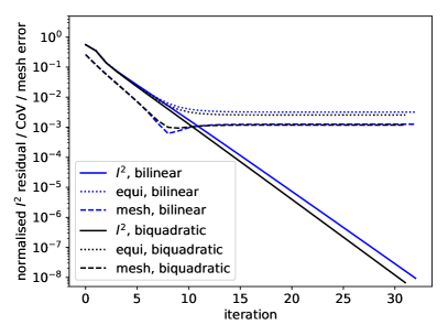
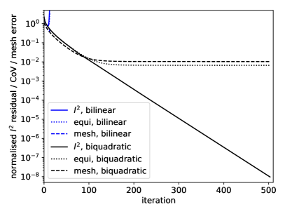
Figure 8: Convergence of diagnostic measures, when using the relaxation method, for the sphere monitor function eq. 5.10. Left: X2 mesh, with $\gamma=(1/2)^{4}$. Right: X16 mesh, with $\gamma=(1/16)^{4}$. In this case, the method diverges when a bilinear representation of the mesh is used (top-left of plot).

The convergence of the relaxation method for X2 and X16 problems, using a cubed-sphere mesh, is shown in fig. 8. For the gentle X2 problem, there is only a small difference between the bilinear and biquadratic mesh representation behaviour. The convergence of the $l^{2}$-norm measure is again linear, and the equidistribution and “exact mesh” error measures converge to some non-zero value. For the extreme X16 problem, we find that the method only converges when using the biquadratic mesh representation. In this case, the convergence behaviour is largely the same as for the X2 problem, although far more iterations are required. The bilinear (lowest-order) mesh initially evolves in the same way, but wildly diverges after just some 10 iterations. In fig. 9 we show the mesh produced at some intermediate iteration when using a bilinear representation, in a tangled state, shortly before complete blow-up occurs.

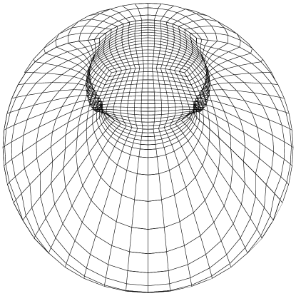
Figure 9: Failure of bilinear mesh representation to create mesh adapted to monitor function eq. 5.10 with $\gamma=(1/16)^{4}$ using relaxation method. Pictured is the mesh generated at an intermediate iteration. The method works successfully with the biquadratic representation; the resulting mesh was shown in fig. 6.

5.2.2 Quasi-Newton method

We also implemented a quasi-Newton scheme for the sphere, similarly as for the plane. Automatic differentiation is used to avoid manually calculating the linearisation of eq. 4.8 for assembling the Jacobian. We study the convergence of the X2, X4, X8 and X16 cubed-sphere meshes.

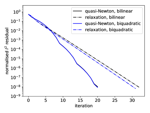
Figure 10: Comparison of the convergence of the quasi-Newton and relaxation methods for the sphere, with the cubed sphere X2 mesh and the monitor function eq. 5.10, with $\gamma=(1/2)^{4}$

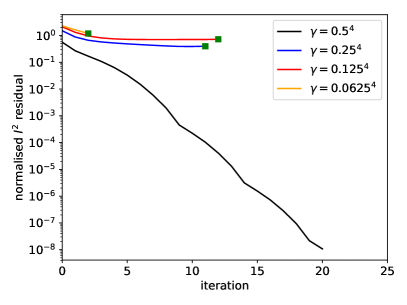
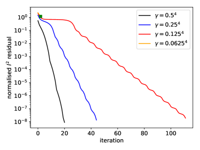
Figure 11: Performance of the quasi-Newton method for creating a cubed-sphere mesh adapted to the monitor function eq. 5.10, for a range of values of $\gamma$. Left: when a bilinear mesh representation is used. Convergence is only achieved for the X2 problem; the green squares denote failure of the nonlinear solver. Right: when a biquadratic mesh representation is used. Convergence is achieved for the X2, X4 and X8 problems, but not for the X16 problem.

We again find that it is essential to use the biquadratic mesh representation. It is only for the simple X2 problem that the bilinear mesh representation also leads to convergence. In fig. 10, we compare the convergence of the quasi-Newton method to the relaxation method in this case. Convergence is reached in about half as many iterations as for the relaxation method, although (as in the plane) each iteration is far more expensive. With the biquadratic mesh representation, we also get convergence for the X4 and X8 cases, though not in the most challenging X16 case, in which the monitor function varies by a factor of 256. This is summarised in fig. 11. The typical failure mode is stagnation of GMRES iterations in the linear solver after a few nonlinear iterations, suggesting the linear problem is not well-posed due to, e.g., loss of convexity. This failure of convergence with the quasi-Newton method for extreme monitor functions is not specific to the sphere. The same occurs on the plane for harsher monitor functions than were presented in section 5.1 (the bell monitor function only varied by a factor of 51).

5.3 Comments

We found the relaxation method is completely robust for generating adapted meshes on the plane, so long as the step size is small enough for the method to be stable. On the sphere, if a lowest-order representation of the mesh is used then the relaxation method fails for moderately-challenging monitor functions. This continues to happen even if the step size is made arbitrary small. However, if a higher-order representation is used (quadratic for triangular meshes, biquadratic for quadrilateral meshes), the method is again completely robust. On both the plane and sphere, the speed of convergence is heavily dependent on the complexity of the monitor function; if $m$ varies by a factor of 100 or 1000 or more, it takes hundreds or thousands of iterations for the method to converge.

The quasi-Newton method is moderately robust on the plane and sphere (assuming a higher-order mesh representation), struggling for only the most challenging monitor functions. The convergence is only first-order, since we only use a partial linearisation when forming the Jacobian, but still converges in far fewer iterations than the relaxation method. The use of a line search allows the method to take smaller steps in the first iterations. Indeed, the quasi-Newton and relaxation methods often initially converge at a similar rate; this is particularly noticeable in fig. 3.

Of course, each iteration of the quasi-Newton method is much more expensive than an iteration of the relaxation method. We refrain from making definitive statements comparing the wall-clock time of the two methods, since we have not put significant effort into optimising our implementations (for example, our preconditioner for the quasi-Newton method can surely be improved, the Firedrake framework assumes an unstructured mesh although our $\tau_{C}$ is partially or fully structured, we use an algebraic multigrid preconditioner rather than geometric, and so on). However, to give a ballpark estimate, we find that one quasi-Newton iteration takes roughly ten times as long as an iteration of the relaxation method. It is therefore clear that the Newton-based method will only dominate the relaxation method if we are able to use a full linearisation to increase the rate of convergence.

5.4 Behaviour with increasing mesh resolution

So far, we have investigated the behaviour of our methods on various monitor functions, but only at a single mesh resolution. In this section, we now perform a series of numerical experiments to investigate the performance of our methods at higher resolution – up to 240 x 240 cells on the plane, and up to 81920 cells on the sphere. In particular, we study the convergence of the method with increasing resolution (via the equidistribution measure), and the computational cost. We confine our attention to two representative examples: the ring monitor function eq. 5.3 on the plane, and the cross monitor function eq. 5.11 on the sphere. In both cases, we see good and regular convergence of the meshes with increasing resolution. There is no evidence whatsoever of mesh tangling or any other form of mesh instability. Close-ups of the finest meshes are shown in fig. 12, and these indeed look very regular.

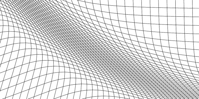
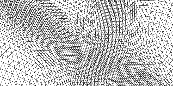
Figure 12: Top: part of a 240 x 240 mesh adapted to the ring monitor function eq. 5.3. Bottom: part of an icosahedral mesh, refined 6 times, adapted to the cross monitor function eq. 5.11. Both pictures show good mesh behaviour, which is evidence that highly-refined meshes generated using our methods do not tangle.

Recall the equidistribution measure that we used earlier: we formed the $M_{i}$ by integrating the monitor function over each cell as in eq. 5.2, then considered the coefficient of variation of these – the standard deviation divided by the mean. We saw in figs. 3 and 8 that (at a given mesh resolution) the nonlinear iterations drive this quantity to some small, but non-zero, value. In fig. 13, we show that this quantity converges to zero as the mesh is refined. Notably, this quantity is proportional to $\Delta x^{2}$ on the plane, but only $\Delta x$ on the sphere. We do not yet have an explanation from first principles for this differing behaviour.

Figure 13: Convergence of the equidistribution measure to zero on the plane and sphere with a sequence of refined meshes. The planar meshes used range from 30 x 30 to 240 x 240, while the spherical meshes are icosahedral meshes refined between 3 and 6 times. The equidistribution measure goes to zero with $\Delta x^{2}$ on the plane, and with $\Delta x$ on the sphere.

Some timings are given in fig. 14 for applying the relaxation and quasi-Newton methods to a range of mesh sizes on the plane and sphere. On the plane, we again use the ring monitor function eq. 5.3, with meshes ranging from 60 x 60 to 240 x 240. On the sphere, we use the cross monitor function eq. 5.11 with icosahedral meshes refined between 3 and 6 times. The timings given are only meant to be indicative; they were measured on a desktop computer with no other significant applications running, but do not represent precise performance measurements. Repeated runs would typically vary by around a percent.

Both methods appear to be $\mathcal{O}(N)$, as expected, where $N$ is the number of mesh cells. For the relaxation method, this is easy to explain: it is essentially a sequence of Poisson solves, which are $\mathcal{O}(N)$ when using a multigrid solver or preconditioner . The number of nonlinear iterations and the maximum ‘stable’ step are then fairly independent of mesh resolution. This may be surprising, but we argue that this is because instability is caused by loss of convexity rather than by the violation of some CFL-like constraint. In more detail, the relaxation method is essentially a forward Euler scheme in some artificial time, per eq. 2.15. This could equally be applied to the continuous-in-space problem, and we believe the maximum stable timestep would be bounded away from zero as long as various derivatives are not unbounded. The discrete problem then inherits the same maximum stable timestep once the monitor function is sufficiently resolved. Conversely, an unstable timestep for a discrete problem would also cause loss of convexity at the continuous level. For the quasi-Newton method, the linear solves are also $\mathcal{O}(N)$ since we use the Riesz map block preconditioning matrix and an AMG preconditioner on the elliptic part of the system. We also observe the nonlinear convergence to be effectively mesh-independent, and there are again parallels with the continuous-in-space problem.

Although these methods are $\mathcal{O}(N)$, the ‘constant’ is higher than we would like. There are at least two mitigating factors. Firstly, the tolerances used are the same as in section 5.1, which are considerably tighter than would be used in practice. For example, if we reduced the tolerance from $10^{-8}$ to $10^{-2}$, the time taken would decrease approximately fourfold. Secondly, if we were doing a true moving mesh simulation, we would have a good ‘initial guess’ available, while in these examples we were always starting from a uniform mesh.

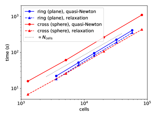
Figure 14: Observed timings for generating meshes adapted to the planar ring monitor function and the spherical cross monitor function, over a range of mesh sizes. Both the relaxation and quasi-Newton methods appear to be $\mathcal{O}(N)$, on both the plane and the sphere.

6 Conclusions and future work

In this paper, we have presented two approaches for solving a nonlinear problem for the generation of optimally-transported meshes on the plane and sphere. The resulting algorithms are robust, particularly the relaxation method. They are well-suited to parallel architectures, since we reduced the mesh generation problem to the numerical solution of a PDE with the finite element method. In all cases, a suitable adapted mesh can be quickly generated following the specification of a scalar mesh density. We give a more detailed analysis of the regularity of such meshes of the sphere in Budd et al. (2017), which extends the results of Budd et al. (2015) on the plane.

We remark that our variety of mesh adaptivity, in which the topology of the mesh must remain fixed, is far from ideal for the monitor functions we used on the sphere. We believe that $r$-adaptivity is best used in the presence of local features, with negligible large-scale distortion of the mesh. However, particularly in the X16 case, the global behaviour was completely dominated by the ‘inner region’; almost all of the mesh cells were pulled in. In these situations, the fixed topology could be a severe hindrance. The fact that our method produces a passable mesh, even in this ‘worst-case’ scenario, is a testament to the robustness of the optimal-transport-based approach. In practice, one is likely to use a regularisation (as proposed in, say, Beckett and Mackenzie (2000)) which modifies the equidistributed monitor function so that this undesirable behaviour does not occur in the first place.

Extending the work in this paper, we expect to improve the convergence rate of the Newton-based approach by using a full linearisation of the residual when forming the Jacobian. This may involve, for example, solving a regularised Monge–Ampère equation whose convexity requirements are less strict. In the longer term, our ultimate aim is to simulate PDEs describing atmospheric flow using $r$-adaptive meshes. This will involve coupling a suitable discretisation strategy for the physical PDEs with moving meshes generated using the methods described in this paper.

Appendix A Exact construction of meshes in the presence of axisymmetric monitor functions

More details of this construction are given in the parallel paper Budd et al. (2017), in which we analyse the regularity of the resulting meshes.

Let $\Omega$ be a sphere centred at the origin. Consider a monitor function which is axisymmetric about an axis $\vec{x_{c}}\in\Omega$. Then

$$m(\vec{x})\equiv M(s),$$ (A.1)

where

$$s\vcentcolon=\|\vec{x}-\vec{x_{c}}\|,$$ (A.2)

is the geodesic distance on the physical mesh. It is clear that the exact map $\vec{x}^{\>e}(\vec{\xi})$ should only move points along geodesics passing through $\vec{x_{c}}$. Define

$$t\vcentcolon=\|\vec{\xi}-\vec{x_{c}}\|,$$ (A.3)

the geodesic distance on the computational mesh. The problem of finding the map $\vec{x}^{\>e}(\vec{\xi})$, and hence the resulting mesh, is therefore reduced to the problem of finding $s(t)$.

From geometrical considerations, the equidistribution condition implies that $s$ and $t$ are linked by the integral identity

$$\int_{0}^{s}M(s^{\prime})\sin(s^{\prime})\,\;\mathrm{d}s^{\prime} =\theta\int_{0}^{t}\sin(t^{\prime})\,\;\mathrm{d}t^{\prime}$$ (A.4)

$$=\theta(1-\cos t),$$ (A.5)

where $\theta$ is a normalisation constant that ensures that the surface of the sphere is mapped to itself, i.e. that $s(0)=0$ and $s(\pi)=\pi$:

$$\theta=\frac{1}{2}\int_{0}^{\pi}M(s^{\prime})\sin(s^{\prime})\,\;\mathrm{d}s^{\prime}.$$ (A.6)

For a given function $M(s)$, $\theta$ can be evaluated to an appropriate degree of accuracy using numerical quadrature. Our algorithm is then the following: for a single computational mesh vertex $\vec{\xi}_{i}$, we evaluate $t$ from eq. A.3. We then obtain the corresponding $s$ using interval bisection, making use of numerical quadrature to evaluate the left-hand-side of eq. A.4. Finally, we generate the mesh point $\vec{x}^{\>e}_{i}$, making use of eq. 4.2.

In our implementation, we use the quadrature and interval bisection routines from SciPy (Jones et al., 2001–). The quadrature is performed with a relative error tolerance of $10^{-7}$, and the interval bisection is performed with a tolerance of $10^{-6}$.

Appendix B Code availability

All of the numerical experiments given in this paper were performed with the following versions of software, which we have archived on Zenodo: Firedrake (Zenodo/Firedrake, ), PyOP2 (Zenodo/PyOP2, ), TSFC (Zenodo/TSFC, ), COFFEE (Zenodo/COFFEE, ), UFL (Zenodo/UFL, ), FInAT (Zenodo/FInAT, ), FIAT (Zenodo/FIAT, ), PETSc (Zenodo/PETSc, ), petsc4py (Zenodo/petsc4py, ). The code for the numerical experiments can be found in the supplementary material to this paper.

References

- Aguilera and Morin (2009) Néstor E. Aguilera and Pedro Morin. On Convex Functions and the Finite Element Method. SIAM Journal on Numerical Analysis, 47(4):3139–3157, 2009. 10.1137/080720917.
- Alnæs et al. (2014) Martin S. Alnæs, Anders Logg, Kristian B. Ølgaard, Marie E. Rognes, and Garth N. Wells. Unified Form Language: A Domain-Specific Language for Weak Formulations of Partial Differential Equations. ACM Transactions on Mathematical Software, 40(2):9:1–9:37, 2014. 10.1145/2566630.
- Awanou (2015) Gerard Awanou. Quadratic mixed finite element approximations of the Monge–Ampère equation in 2D. Calcolo, 52(4):503–518, 2015. 10.1007/s10092-014-0127-7.
- Balay et al. (1997) Satish Balay, William D. Gropp, Lois Curfman McInnes, and Barry F. Smith. Efficient Management of Parallelism in Object Oriented Numerical Software Libraries. In E. Arge, A. M. Bruaset, and H. P. Langtangen, editors, Modern Software Tools in Scientific Computing, pages 163–202. Birkhäuser Press, 1997.
- Balay et al. (2016) Satish Balay, Shrirang Abhyankar, Mark F. Adams, Jed Brown, Peter Brune, Kris Buschelman, Lisandro Dalcin, Victor Eijkhout, William D. Gropp, Dinesh Kaushik, Matthew G. Knepley, Lois Curfman McInnes, Karl Rupp, Barry F. Smith, Stefano Zampini, Hong Zhang, and Hong Zhang. PETSc Users Manual. Technical Report ANL-95/11 - Revision 3.7, Argonne National Laboratory, 2016. URL http://www.mcs.anl.gov/petsc.
- Beckett and Mackenzie (2000) G. Beckett and J.A. Mackenzie. Convergence analysis of finite difference approximations on equidistributed grids to a singularly perturbed boundary value problem. Applied Numerical Mathematics, 35(2):87–109, 2000. 10.1016/S0168-9274(99)00065-3.
- Benamou et al. (2010) Jean-David Benamou, Brittany D. Froese, and Adam M. Oberman. Two Numerical Methods for the Elliptic Monge-Ampère Equation. ESAIM: Mathematical Modelling and Numerical Analysis, 44(4):737–758, 2010. 10.1051/m2an/2010017.
- Benamou et al. (2014) Jean-David Benamou, Brittany D. Froese, and Adam M. Oberman. Numerical solution of the Optimal Transportation problem using the Monge–Ampère equation. Journal of Computational Physics, 260:107–126, 2014. 10.1016/j.jcp.2013.12.015.
- Bernsen et al. (2006) Erik Bernsen, Onno Bokhove, and Jaap J.W. van der Vegt. A (Dis)continuous finite element model for generalized 2D vorticity dynamics. Journal of Computational Physics, 211(2):719–747, 2006. 10.1016/j.jcp.2005.06.008.
- Brenier (1991) Yann Brenier. Polar Factorization and Monotone Rearrangement of Vector-Valued Functions. Communications on Pure and Applied Mathematics, 44(4):375–417, 1991. 10.1002/cpa.3160440402.
- Brenner et al. (2011) Susanne C. Brenner, Thirupathi Gudi, Michael Neilan, and Li-yeng Sung. penalty methods for the fully nonlinear Monge-Ampère equation. Mathematics of Computation, 80(276):1979–1995, 2011. 10.1090/S0025-5718-2011-02487-7.
- Brenner and Neilan (2012) Susanne Cecelia Brenner and Michael Neilan. Finite element approximations of the three dimensional Monge-Ampère equation. ESAIM: Mathematical Modelling and Numerical Analysis, 46(5):979–1001, 2012. 10.1051/m2an/2011067.
- Brown et al. (2012) Jed Brown, Matthew G. Knepley, David A. May, Lois Curfman McInnes, and Barry Smith. Composable Linear Solvers for Multiphysics. In 2012 11th International Symposium on Parallel and Distributed Computing, pages 55–62, 2012. ISBN 978-1-4673-2599-8. 10.1109/ISPDC.2012.16.
- Browne et al. (2014) P.A. Browne, C.J. Budd, C. Piccolo, and M. Cullen. Fast three dimensional r-adaptive mesh redistribution. Journal of Computational Physics, 275:174–196, 2014. 10.1016/j.jcp.2014.06.009.
- Browne et al. (2016) P.A. Browne, J. Prettyman, H. Weller, T. Pryer, and J. Van lent. Nonlinear solution techniques for solving a Monge-Ampère equation for redistribution of a mesh. 2016. URL https://arxiv.org/abs/1609.09646.
- Brune et al. (2015) Peter R. Brune, Matthew G. Knepley, Barry F. Smith, and Xuemin Tu. Composing Scalable Nonlinear Algebraic Solvers. SIAM Review, 57(4):535–565, 2015. 10.1137/130936725.
- Budd and Williams (2006) C J Budd and J F Williams. Parabolic Monge–Ampère methods for blow-up problems in several spatial dimensions. Journal of Physics A: Mathematical and General, 39(19):5425–5444, 2006. 10.1088/0305-4470/39/19/S06.
- Budd and Williams (2009) C. J. Budd and J. F. Williams. Moving Mesh Generation Using the Parabolic Monge–Ampère Equation. SIAM Journal on Scientific Computing, 31(5):3438–3465, 2009. 10.1137/080716773.
- Budd et al. (2009) Chris J. Budd, Weizhang Huang, and Robert D. Russell. Adaptivity with moving grids. Acta Numerica, 18:111–241, 2009. 10.1017/S0962492906400015.
- Budd et al. (2017) Chris J. Budd, Andrew T. T. McRae, and Colin J. Cotter. The geometry of optimally transported meshes on the sphere. Submitted to Journal of Computational Physics, 2017. URL https://arxiv.org/abs/1711.00260.
- Budd et al. (2013) C.J. Budd, M.J.P. Cullen, and E.J. Walsh. Monge–Ampére based moving mesh methods for numerical weather prediction, with applications to the Eady problem. Journal of Computational Physics, 236:247–270, 2013. 10.1016/j.jcp.2012.11.014.
- Budd et al. (2015) C.J. Budd, R.D. Russell, and E. Walsh. The geometry of r-adaptive meshes generated using optimal transport methods. Journal of Computational Physics, 282:113–137, 2015. 10.1016/j.jcp.2014.11.007.
- Chacón et al. (2011) L. Chacón, G.L. Delzanno, and J.M. Finn. Robust, multidimensional mesh-motion based on Monge–Kantorovich equidistribution. Journal of Computational Physics, 230(1):87–103, 2011. 10.1016/j.jcp.2010.09.013.
- Dalcin et al. (2011) Lisandro D. Dalcin, Rodrigo R. Paz, Pablo A. Kler, and Alejandro Cosimo. Parallel distributed computing using Python. Advances in Water Resources, 34(9):1124–1139, 2011. 10.1016/j.advwatres.2011.04.013.
- Dean and Glowinski (2006a) E. J. Dean and R. Glowinski. An augmented Lagrangian approach to the numerical solution of the Dirichlet problem for the elliptic Monge-Ampère equation in two dimensions. Electronic Transactions on Numerical Analysis, 22:71–96, 2006a.
- Dean and Glowinski (2006b) E.J. Dean and R. Glowinski. Numerical methods for fully nonlinear elliptic equations of the Monge–Ampère type. Computer Methods in Applied Mechanics and Engineering, 195(13-16):1344–1386, 2006b. 10.1016/j.cma.2005.05.023.
- Delzanno and Finn (2010) G. L. Delzanno and J. M. Finn. Generalized Monge–Kantorovich Optimization for Grid Generation and Adaptation in . SIAM Journal on Scientific Computing, 32(6):3524–3547, 2010. 10.1137/090749785.
- Delzanno et al. (2008) G.L. Delzanno, L. Chacón, J.M. Finn, Y. Chung, and G. Lapenta. An optimal robust equidistribution method for two-dimensional grid adaptation based on Monge–Kantorovich optimization. Journal of Computational Physics, 227(23):9841–9864, 2008. 10.1016/j.jcp.2008.07.020.
- Dietachmayer and Droegemeier (1992) Gary S. Dietachmayer and Kelvin K. Droegemeier. Application of Continuous Dynamic Grid Adaption Techniques to Meteorological Modeling. Part I: Basic Formulation and Accuracy. Monthly Weather Review, 120(8):1675–1706, 1992. 10.1175/1520-0493(1992)120¡1675:AOCDGA¿2.0.CO;2.
- Feng and Neilan (2009) Xiaobing Feng and Michael Neilan. Mixed Finite Element Methods for the Fully Nonlinear Monge–Ampère Equation Based on the Vanishing Moment Method. SIAM Journal on Numerical Analysis, 47(2):1226–1250, 2009. 10.1137/070710378.
- Froese and Oberman (2011a) B.D. Froese and A.M. Oberman. Fast finite difference solvers for singular solutions of the elliptic Monge–Ampère equation. Journal of Computational Physics, 230(3):818–834, 2011a. 10.1016/j.jcp.2010.10.020.
- Froese and Oberman (2011b) Brittany D. Froese and Adam M. Oberman. Convergent Finite Difference Solvers for Viscosity Solutions of the Elliptic Monge–Ampère Equation in Dimensions Two and Higher. SIAM Journal on Numerical Analysis, 49(4):1692–1714, 2011b. 10.1137/100803092.
- Homolya and Ham (2016) M. Homolya and D. A. Ham. A parallel edge orientation algorithm for quadrilateral meshes. SIAM Journal on Scientific Computing, 38(5):S48–S61, 2016. 10.1137/15M1021325.
- Homolya et al. (2017a) Miklós Homolya, Robert C. Kirby, and David A. Ham. Exposing and exploiting structure: optimal code generation for high-order finite element methods. Submitted to ACM Transactions on Mathematical Software, 2017a. URL https://arxiv.org/abs/1711.02473.
- Homolya et al. (2017b) Miklós Homolya, Lawrence Mitchell, Fabio Luporini, and David A. Ham. TSFC: a structure-preserving form compiler. Submitted to SIAM Journal on Scientific Computing, 2017b. URL https://arxiv.org/abs/1705.03667.
- Huang and Russell (2011) Weizhang Huang and Robert D. Russell. Adaptive Moving Mesh Methods. Applied Mathematical Sciences. Springer Science+Business Media, LLC, 2011. ISBN 978-1-4419-7915-5. 10.1007/978-1-4419-7916-2.
- Jones et al. (2001–) Eric Jones, Travis Oliphant, Pearu Peterson, et al. SciPy: Open Source Scientific Tools for Python, 2001–. URL http://www.scipy.org/. [Online; accessed 2017-06-26].
- Kühnlein et al. (2012) Christian Kühnlein, Piotr K. Smolarkiewicz, and Andreas Dörnbrack. Modelling atmospheric flows with adaptive moving meshes. Journal of Computational Physics, 231(7):2741–2763, 2012. 10.1016/j.jcp.2011.12.012.
- Lakkis and Pryer (2011) Omar Lakkis and Tristan Pryer. A Finite Element Method for Second Order Nonvariational Elliptic Problems. SIAM Journal on Scientific Computing, 33(2):786–801, 2011. 10.1137/100787672.
- Lakkis and Pryer (2013) Omar Lakkis and Tristan Pryer. A Finite Element Method for Nonlinear Elliptic Problems. SIAM Journal on Scientific Computing, 35(4):A2025–A2045, 2013. 10.1137/120887655.
- Loeper and Rapetti (2005) Grégoire Loeper and Francesca Rapetti. Numerical solution of the Monge–Ampère equation by a Newton’s algorithm. Comptes Rendus Mathematique, 340(4):319–324, 2005. 10.1016/j.crma.2004.12.018.
- Luporini et al. (2017) Fabio Luporini, David A. Ham, and Paul H. J. Kelly. An algorithm for the optimization of finite element integration loops. ACM Transactions on Mathematical Software, 44(1):3:1–3:26, 2017. 10.1145/3054944.
- Mardal and Winther (2011) Kent-Andre Mardal and Ragnar Winther. Preconditioning discretizations of systems of partial differential equations. Numerical Linear Algebra with Applications, 18(1):1–40, 2011. 10.1002/nla.716.
- McCann (2001) Robert J. McCann. Polar factorization of maps on Riemannian manifolds. Geometric And Functional Analysis, 11(3):589–608, 2001. 10.1007/PL00001679.
- McRae et al. (2016) A. T. T. McRae, G.-T. Bercea, L. Mitchell, D. A. Ham, and C. J. Cotter. Automated generation and symbolic manipulation of tensor product finite elements. SIAM Journal on Scientific Computing, 38(5):S25–S47, 2016. 10.1137/15M1021167.
- Neilan (2014) Michael Neilan. Finite element methods for fully nonlinear second order PDEs based on a discrete Hessian with applications to the Monge–Ampère equation. Journal of Computational and Applied Mathematics, 263:351–369, 2014. 10.1016/j.cam.2013.12.027.
- Oliker and Prussner (1989) V.I. Oliker and L.D. Prussner. On the Numerical Solution of the Equation and Its Discretizations, I. Numerische Mathematik, 54(3):271–293, 1989. 10.1007/BF01396762.
- Piccolo and Cullen (2011) Chiara Piccolo and Mike Cullen. Adaptive mesh method in the Met Office variational data assimilation system. Quarterly Journal of the Royal Meteorological Society, 137(656):631–640, 2011. 10.1002/qj.801.
- Piccolo and Cullen (2012) Chiara Piccolo and Mike Cullen. A new implementation of the adaptive mesh transform in the Met Office 3D-Var System. Quarterly Journal of the Royal Meteorological Society, 138(667):1560–1570, 2012. 10.1002/qj.1880.
- Prusa and Smolarkiewicz (2003) Joseph M. Prusa and Piotr K. Smolarkiewicz. An all-scale anelastic model for geophysical flows: dynamic grid deformation. Journal of Computational Physics, 190(2):601–622, 2003. 10.1016/S0021-9991(03)00299-7.
- Rathgeber et al. (2016) Florian Rathgeber, David A. Ham, Lawrence Mitchell, Michael Lange, Fabio Luporini, Andrew T. T. McRae, Gheorghe-Teodor Bercea, Graham R. Markall, and Paul H. J. Kelly. Firedrake: Automating the Finite Element Method by Composing Abstractions. ACM Transactions on Mathematical Software, 43(3):24:1–24:27, 2016. 10.1145/2998441.
- Ringler et al. (2011) Todd D. Ringler, Doug Jacobsen, Max Gunzburger, Lili Ju, Michael Duda, and William Skamarock. Exploring a Multiresolution Modeling Approach within the Shallow-Water Equations. Monthly Weather Review, 139(11):3348–3368, 2011. 10.1175/MWR-D-10-05049.1.
- Rognes et al. (2013) M. E. Rognes, D. A. Ham, C. J. Cotter, and A. T. T. McRae. Automating the solution of PDEs on the sphere and other manifolds in FEniCS 1.2. Geoscientific Model Development, 6(6):2099–2119, 2013. 10.5194/gmd-6-2099-2013.
- Shu and Osher (1988) Chi-Wang Shu and Stanley Osher. Efficient Implementation of Essentially Non-oscillatory Shock-Capturing Schemes. Journal of Computational Physics, 77(2):439–471, 1988. 10.1016/0021-9991(88)90177-5.
- Smolarkiewicz and Prusa (2005) Piotr K. Smolarkiewicz and Joseph M. Prusa. Towards mesh adaptivity for geophysical turbulence: continuous mapping approach. International Journal for Numerical Methods in Fluids, 47(8-9):789–801, 2005. 10.1002/fld.858.
- Sulman et al. (2011) Mohamed Sulman, J.F. Williams, and R.D. Russell. Optimal mass transport for higher dimensional adaptive grid generation. Journal of Computational Physics, 230(9):3302–3330, 2011. 10.1016/j.jcp.2011.01.025.
- Weller et al. (2016) Hilary Weller, Philip Browne, Chris Budd, and Mike Cullen. Mesh adaptation on the sphere using optimal transport and the numerical solution of a Monge–Ampère type equation. Journal of Computational Physics, 308:102–123, 2016. 10.1016/j.jcp.2015.12.018.
- (58) Zenodo/COFFEE. COFFEE: A Compiler for Fast Expression Evaluation, November 2017. URL https://doi.org/10.5281/zenodo.1064647.
- (59) Zenodo/FIAT. FIAT: The Finite Element Automated Tabulator, November 2017. URL https://doi.org/10.5281/zenodo.1043841.
- (60) Zenodo/FInAT. FInAT: a smarter library of finite elements, October 2017. URL https://doi.org/10.5281/zenodo.1039605.
- (61) Zenodo/Firedrake. Firedrake: an automated finite element system, November 2017. URL https://doi.org/10.5281/zenodo.1064234.
- (62) Zenodo/PETSc. PETSc: Portable, Extensible Toolkit for Scientific Computation, October 2017. URL https://doi.org/10.5281/zenodo.1022071.
- (63) Zenodo/petsc4py. petsc4py: The Python interface to PETSc, October 2017. URL https://doi.org/10.5281/zenodo.1022068.
- (64) Zenodo/PyOP2. PyOP2: Framework for performance-portable parallel computations on unstructured meshes, November 2017. URL https://doi.org/10.5281/zenodo.1043839.
- (65) Zenodo/TSFC. TSFC: The Two Stage Form Compiler, November 2017. URL https://doi.org/10.5281/zenodo.1064746.
- (66) Zenodo/UFL. UFL: The Unified Form Language, November 2017. URL https://doi.org/10.5281/zenodo.1043842.