Node aware sparse matrix-vector multiplication

Abstract

The sparse matrix-vector multiply (SpMV) operation is a key computational kernel in many simulations and linear solvers. The large communication requirements associated with a reference implementation of a parallel SpMV result in poor parallel scalability. The cost of communication depends on the physical locations of the send and receive processes: messages injected into the network are more costly than messages sent between processes on the same node. In this paper, a node aware parallel SpMV (NAPSpMV) is introduced to exploit knowledge of the system topology, specifically the node-processor layout, to reduce costs associated with communication. The values of the input vector are redistributed to minimize both the number and the size of messages that are injected into the network during a SpMV, leading to a reduction in communication costs. A variety of computational experiments that highlight the efficiency of this approach are presented.

1 Introduction

The sparse matrix-vector multiply (SpMV) is a widely used operation in many simulations and the main kernel in iterative solvers. The focus of this paper is on the parallel SpMV, namely

$$w\leftarrow A\cdot v\\$$ (1)

where $A$ is a sparse $N\times N$ matrix and $v$ is a dense $N$-dimensional vector. In parallel, the sparse system is often distributed across $n_{p}$ processes such that each process holds a contiguous block of rows from the matrix $A$, and equivalent rows from the vectors $v$ and $w$, as shown in Figure 1. A common approach is to also split the rows of $A$ on a single process into two groups: an on-process block, containing the columns of the matrix that correspond to vector values stored locally, and an off-process block, containing matrix non-zeros that are associated with vector values that are stored on non-local processes. Therefore, non-zeros in the off-process block of the matrix require vector values to be communicated during each SpMV.

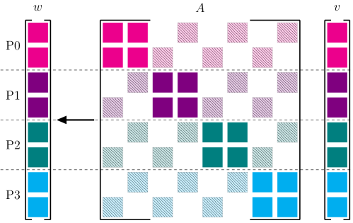
Figure 1: A matrix partitioned across four processes, where each process stores two rows of the matrix, and the equivalent rows of each vector. The on-process block of each matrix partition is represented by solid squares, while the off-process block is represented by patterned entries.

The SpMV operation lacks parallel scalability due to large costs associated with communication, specifically in the strong scaling limit of a few rows per process. Increasing the number of processes that a matrix is distributed across increases the number of columns in the off-process blocks, yielding a growth in communication.

Figure 2 shows the percentage of time spent communicating during a SpMV operation for two large matrices from the SuiteSparse matrix collection at scales varying from $50\,000$ to $500\,000$ non-zeros per process [1]. The results show that the communication time dominates the computation as the number of processes is increased, thus decreasing the scalability.

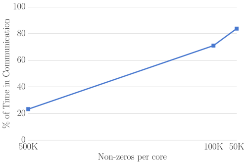
Figure 2: Percentage of total SpMV time spent during communication for matrix nlpkkt240 with 760,648,352 non-zeros

Machine topology plays an important role in the cost of communication [2]. Multicore distributed systems present new challenges in communication as the bandwidth is limited while the number of cores participating in communication increases [3]. Injection limits and network contention are significant roadblocks in the SpMV operation, motivating the need for SpMV algorithms that take advantage of the machine topology. The focus of the approach developed in this paper is to use the node-processor hierarchy to more efficiently map communication, leading to notable reductions in SpMV costs on modern HPC systems for a range of sparse matrix patterns. Throughout this paper, the term node aware refers to knowledge of the mapping of processes to physical nodes, although other aspects of the topology — e.g. socket information — could be used in a similar fashion. The mapping of virtual ranks to physical processors can be easily determined on many super computers. The flag MPICH_RANK_REORDER_METHOD can be set to a predetermined ordering on Cray machines, while modern Blue Gene machines allow the user to specify the ordering among the coordinates A, B, C, D, E, and T through the variable RUNJOB_MAPPING or a runscript option of --mapping.

There are a number of existing approaches for reducing communication costs associated with sparse matrix-vector multiplication. Communication volume in particular is a limiting factor and the ordering and parallel partition of a matrix both influence the total data volume. In response, graph partitioning techniques are used to identify more efficient layouts in the data [4, 5, 6, 7]. ParMETIS [8] and PT-Scotch [9], for example, provide parallel partitioning of matrices that often lead to improved system loads and more efficient sparse matrix operations. Communication volume is accurately modeled through the use of a hypergraph [10]. As a result, hypergraph partitioning also leads to a reduction in parallel communication requirements, albeit at a larger one-time setup cost. Topology-aware task mapping is used to accurately map partitions to the allocated nodes of a supercomputer, reducing the overall cost associated with communication [11, 12, 13, 14, 15]. The approach introduced in this paper complements these efforts by providing an additional level of optimization in handling communication.

Topology-aware methods and aggregation of data are commmonly used to reduce communication costs, particularly in collective operations [16, 17, 18, 19]. Aggregation of data is used in point to point communication through Tram, a library for streamlining messages in which data is aggregated and communicated only through neighboring processors [20]. The method presented in this paper aggregates messages at the node level and communicates all aggregated data at once, yielding little structural change from standard MPI communication while reducing overall cost.

The performance of matrix operations can also be improved through the use of hybrid architectures and accelerators, such a graphics processing units (GPUs). The throughput of GPUs allows for improved performance when memory access patterns are optimized [21, 22].

Many preconditioners for iterative methods, such as algebraic multigrid, rely on the SpMV as a dominant operation and therefore lack scalability due to large communication costs. A variety of methods exist for altering the preconditioning algorithms to reduce the communication costs associated with each SpMV [23, 24, 25].

This paper focuses on increasing the locality of communication during a SpMV to reduce the amount of communication injected into the network. Section 2 describes a reference algorithm for a parallel SpMV, which resembles the approach commonly used in practice. A performance model is also introduced in Section 3, which considers the cost of intra- and inter-node communication and the impact on performance. A new SpMV algorithm is presented in Section 4, which reduces the number and size of inter-node messages by increasing the significantly cheaper intra-node communication. The code and numerics are presented in Section 5 to verify the performance.

2 Background

Modern supercomputers incorporate a large number of nodes through an interconnect to form a multi-dimensional grid or torus network. Standard compute nodes are comprised of one or more multicore processors that share a large memory bank. The algorithm developed in this paper targets a general machine with this layout and the results are highlighted on Blue Waters, a Cray machine at the National Center for Supercomputing Applications. Blue Waters consists of $22\,640$ Cray XE nodes, each containing two AMD 6276 Interlagos processors for a total of 16 cores per node, and $4\,228$ Cray XK nodes consisting of a single AMD processor along with an NVIDIA Kepler GPU. The nodes are connected through a three-dimensional torus Gemini interconnect, with each Gemini serving two nodes. The remainder of this paper with focus on only the Cray XE nodes within Blue Waters.

Consider a system with $n_{p}$ processes distributed across $n_{n}$ nodes, resulting in ppn processes per node. Rank $r\in\left[0,n_{p}-1\right]$ is described by the tuple $(p,n)$ where $0\leq p<\textnormal{{ppn}}$ is the local process number of rank $r$ on node $n$. Assuming SMP-style ordering, the first ppn ranks are mapped to the first node, the next ppn to the second node, and so on. Therefore, rank $r$ is described by the tuple $\left(r\mod\textnormal{{ppn}},\lfloor\frac{r}{\textnormal{{ppn}}}\rfloor\right)$. Thus, for the remainder of the paper, the notation of rank $r$ is interchangeable with $\left(p,n\right)$.

Parallel matrices and vectors are distributed across all $n_{p}$ ranks such that each process holds a portion of the linear system. Let $\mathcal{R}(r)$ be the rows of an $N\times N$ sparse linear system, $w\leftarrow A\cdot v$, stored on rank $r$. In the case of an even, contiguous partition where the $k^{\text{th}}$ partition is placed on the $k^{th}$ rank, $\mathcal{R}(r)$ is defined as

$$\mathcal{R}(r) =\left\{\left\lfloor\frac{N}{n_{p}}\right\rfloor r,\ldots,\left\lfloor\frac{N}{n_{p}}\right\rfloor(r+1)-1\right\}$$ (2)

or equivalently as

$$\mathcal{R}((p,n)) =\left\{\left\lfloor\frac{N}{n_{p}}\right\rfloor(p,n),\ldots,\left\lfloor\frac{N}{n_{p}}\right\rfloor((p,n)+1)-1\right\}.$$ (3)

The rows of a matrix $A$ are partitioned into on-process and off-process blocks, as described in Section 1. Accounting for parallel nodal awareness, the off-process block is further partitioned into on-node and off-node blocks, as described in Example 2.1.

Example 2.1

Suppose the parallel system consists of six processes distributed across three nodes, as displayed in Figure 3.

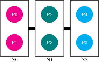
Figure 3: An example parallel system with six processes distributed across three nodes.

Let the linear system $w\leftarrow A\cdot v$ displayed in Figure 4 be partitioned across this processor layout with each process holding a single row of the matrix and associated row of the input vector.

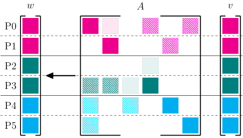
Figure 4: An example $6\times 6$ sparse matrix for the parallel system in Figure 3. The solid shading denotes blocks that require only on-node communication, while the striped shading denotes blocks that require communication with distant nodes.

In this example, the diagonal entry falls into the on-process block, as the corresponding vector value is stored locally. The off-process block, which requires communication, consists of all off-diagonal non-zeros as the associated vector values are stored on other processes.

For any process $(p,n)$, the on-node columns of $A$ correspond to vector values that are stored on some process $(s,n)$, where $s\neq p$. Similarly, the off-node columns of $A$ correspond to vector values stored on some process $(q,m)$, where $m\neq n$. To make this clearer, we define the following

$$\texttt{on\_process}(A,(p,n)) =\left\{A_{ij}\neq 0\,\middle|\,i,j\in\mathcal{R}((p,n))\right\}$$ (4)

$$\texttt{off\_process}(A,(p,n))=\\ \left\{A_{ij}\neq 0\,\middle|\,i\in\mathcal{R}((p,n)),j\not\in\mathcal{R}((p,n))\right\}$$ (5)

$$\texttt{on\_node}(A,(p,n))=\\ \left\{A_{ij}\neq 0\,\middle|\,\exists\,q\neq p\,\textnormal{with $i\in\ \mathcal{R}((p,n))$, $j\in\ \mathcal{R}((q,n))$}\right\}$$ (6)

and

$$\texttt{off\_node}(A,(p,n))=\\ \left\{A_{ij}\neq 0\,\middle|\,\exists\,q,m\neq n\,\textnormal{with $i\in\ \mathcal{R}((p,n))$, $j\in\ \mathcal{R}((q,m))$}\right\}.$$ (7)

2.1 Standard SpMV

For a sparse matrix-vector multiply, $w\leftarrow A\cdot v$, each process receives all values of $v$ associated with the non-zero entries in the off-process block of $A$. For example, if rank $r$ contains a non-zero entry of $A$, $A_{ij}$, at row $i$, column $j$, then rank $s$ with row $j\in\mathcal{R}(s)$ sends the $j^{\text{th}}$ vector value, $v_{j}$, to rank $r$. Typically, these communication requirements are determined as the sparse matrix is formed [26, 27, 28].

In the reference SpMV, for each rank $r$ there is a list of processes to which data is sent, as well as the global vector indices to be sent to each. The function $\mathcal{P}(r)$ defines the list of processes to which a rank $r$ sends. Specifically,

$$\mathcal{P}(r)=\left\{t\,\middle|\,\textnormal{$A_{ij}\neq\ 0$ with $i\in\mathcal{R}{(t)}$, $j\in\mathcal{R}{(r)},\ r\neq t$}\right\}$$ (8)

For each $t$ in $\mathcal{P}(r)$, define the function $\mathcal{D}(r,t)$ to return the global vector indices that process $r$ sends to process $t$. This function is defined as follows.

$$\mathcal{D}(r,t)=\left\{i\,\middle|\,\textnormal{$A_{ij}\neq\ 0$ with $i\in\mathcal{R}{(t)}$, $j\in\mathcal{R}{(r)},\ r\neq t$}\right\}$$ (9)

Consider a standard SpMV for the linear system described in Example 2.1. Table 1 lists the processes to which each rank must send, while Table 2 displays the indices that each rank $r$ sends to any rank $t$.

	$r$
	0	1	2	3	4	5
$\mathcal{P}(r)$	$\left\{3,4,5\right\}$	$\left\{0,3\right\}$	$\left\{3,4\right\}$	$\left\{0,2\right\}$	$\left\{1\right\}$	$\left\{0\right\}$

Table 1: Communication pattern for rank $r$ in Example 2.1, containing the values for $\mathcal{P}(r)$.

.

		$r$
		0	1	2	3	4	5
$t$	0	$\left\{\right\}$	$\left\{1\right\}$	$\left\{\right\}$	$\left\{3\right\}$	$\left\{\right\}$	$\left\{5\right\}$
	1	$\left\{\right\}$	$\left\{\right\}$	$\left\{\right\}$	$\left\{\right\}$	$\left\{4\right\}$	$\left\{\right\}$
	2	$\left\{\right\}$	$\left\{\right\}$	$\left\{\right\}$	$\left\{3\right\}$	$\left\{\right\}$	$\left\{\right\}$
	3	$\left\{0\right\}$	$\left\{1\right\}$	$\left\{2\right\}$	$\left\{\right\}$	$\left\{\right\}$	$\left\{\right\}$
	4	$\left\{0\right\}$	$\left\{\right\}$	$\left\{2\right\}$	$\left\{\right\}$	$\left\{\right\}$	$\left\{\right\}$
	5	$\left\{0\right\}$	$\left\{\right\}$	$\left\{\right\}$	$\left\{\right\}$	$\left\{\right\}$	$\left\{\right\}$

Table 2: Each column $r$ lists the indices of values sent to each process $t$ in $\mathcal{P}(r)$, namely $\mathcal{D}(r,s)$.

.

With these definitions, the standard or reference SpMV is described in Algorithm 1. It is important to note that the parallel communication in Algorithm 1 is executed independent of any locality in the problem. That is, messages sent to another process may be both on-node or off-node depending on the process, however this is not considered in the algorithm.

Input:

$r$

$A|_{\mathcal{R}(r)}$

$v|_{\mathcal{R}(r)}$

Output:

$w|_{\mathcal{R}(r)}$

$A_{\text{on\_process}}={\textnormal{{on\_process}}}(A|_{\mathcal{R}(r)})$

$A_{\text{off\_process}}={\textnormal{{off\_process}}}(A|_{\mathcal{R}(r)})$

for $t\in\mathcal{P}(r)$ do

       for $i\in\mathcal{D}(r,t)$ do

             $b_{\text{send}}\leftarrow v|_{\mathcal{R}{(r)}_{i}}$

            

      ${\textnormal{{MPI\_Isend}}}(b_{\text{send}},\ldots,t,\ldots)$

      

$b_{\text{recv}}\leftarrow\emptyset$

for $t$ s.t. $r\in\mathcal{P}(t)$ do

       ${\textnormal{{MPI\_Irecv}}}(b_{\text{recv}},\ldots,t,\ldots)$

      

${\textnormal{{local\_spmv}}}(A_{\text{on\_process}},v|_{\mathcal{R}(r)})$

MPI_Waitall

${\textnormal{{local\_spmv}}}(A_{\text{off\_process}},b_{\text{recv}})$

Algorithm 1 standard_spmv

3 Communication Models

The performance of Algorithm 1 is sub-optimal since it does not take advantage of node locality in the communication. To see this, a communication performance model is developed in this section. One approach is that of the max-rate model [3], which describes the communication time as

$$T=\alpha+\frac{\textnormal{{ppn}}\cdot s}{\min(B_{\text{N}},B_{\text{max}}+(\textnormal{{ppn}}-1)B_{\text{inj}})},$$ (10)

where $\alpha$ is the latency or start-up cost of a message, which may include preparing a message for transport or determining the network route; $s$ is the number of bytes to be communicated; ppn is again the number of communicating processes per node; $B_{\text{inj}}$ is the maximum rate at which messages are injected into the network; $B_{\max}$ is the achievable message rate of each process or bandwidth; and $B_{\text{N}}$ is the peak rate of the network interface controller (NIC). In the simplest case of $\textnormal{{ppn}}=1$, the familiar postal model suffices:

$$T=\alpha+\frac{s}{B_{\max}}.$$ (11)

MPI contains multiple message passing protocols, including short, eager, and rendezvous. Each message consists of an envelope, including information about the message such as message size and source information, as well as message data. Short messages contain very little data which is sent as part of the envelope. Eager and rendezvous messages, however, send the envelope followed by packets of data. Eager messages are sent under the assumption that the receiving process has buffer space available to store data that is communicated. Therefore, a message is sent without checking buffer space at the receiving process, limiting the associated latency. However, if a message is sufficiently large, rendezvous protocol must be used. This protocol requires the sending process to inform the receiving rank of the message so that buffer space is allocated. The message is sent only once the sending process is informed that this space is available. Therefore, there is a larger overhead with sending a message using rendezvous protocol. Table 3 displays the measurements for $\alpha$, $B_{\text{inj}}$, $B_{\max}$, and $B_{\text{N}}$ for Blue Waters, as determined for the max-rate model.

	$\alpha$	$B_{\text{inj}}$	$B_{\max}$	$B_{\text{N}}$
Short	$4.0\cdot 10^{-6}$	$6.3\cdot 10^{8}$	$-1.8\cdot 10^{7}$	$\infty$
Eager	$1.1\cdot 10^{-5}$	$1.7\cdot 10^{9}$	$6.2\cdot 10^{7}$	$\infty$
Rend	$2.0\cdot 10^{-5}$	$3.6\cdot 10^{9}$	$6.1\cdot 10^{8}$	$5.5\cdot 10^{9}$

Table 3: Measurements for $\alpha$, $B_{\text{inj}}$, $B_{\min}$, and $B_{\text{N}}$ for Blue Waters.

The max-rate model can be improved by distinguishing between intra- and inter-node communication. If the sending and receiving processes lie on the same physical node, data is not injected into the network, yielding low start-up and byte transport costs. As intra-node messages are not injected into the network, communication local to a node can be modeled as

$$T_{\ell}=\alpha_{\ell}+\frac{s_{\ell}}{B_{\max_{\ell}}},$$ (12)

where $\alpha_{\ell}$ is the start-up cost for intra-node messages; $s_{\ell}$ is the number of bytes to be transported; and $B_{\max_{\ell}}$ is the achievable intra-node message rate.

Nodecomm, a topology-aware communication program, measures the time required to communicate on various levels of the parallel system, such as between two nodes of varying distances and between processes local to a node. Communication tests between processes local to one node were used to calculate the intra-node model parameters, as displayed in Table 4.

	$\alpha_{\ell}$	$B_{\max_{\ell}}$
Short	$1.3\cdot 10^{-6}$	$4.2\cdot 10^{8}$
Eager	$1.6\cdot 10^{-6}$	$7.4\cdot 10^{8}$
Rend	$4.2\cdot 10^{-6}$	$3.1\cdot 10^{9}$

Table 4: Measurements for intra-node variables, $\alpha_{\ell}$ and $B_{\max_{\ell}}$.

Furthermore, Figure 5 shows the time required to send a single message of varying sizes. The thin lines display Nodecomm measurements for time required to send a single message, as either inter- or intra-node communication. Furthermore, the thick lines represent the time required to send a message of each size, according to the max-rate model in (10) and intra-node model in (12). This figure displays a significant difference between the costs of intra- and inter-node communication.

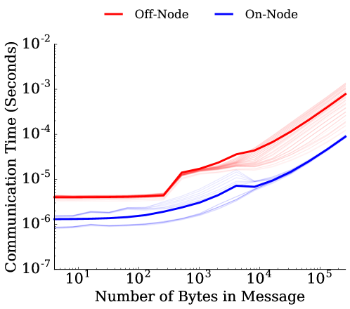
Figure 5: The time required to send a single message of various sizes, with the thin lines representing timings measured by Nodecomm and the thick lines displaying the max-rate and intra-node models in (10) and (12), respectively.

4 Node Aware Parallel SpMV

To reduce communication costs, the algorithm proposed in this section decreases the number and size of messages being injected into the network by increasing the amount of intra-node communication, which is less-costly than inter-node communication. This trade-off is accomplished through a so-called node aware parallel SpMV (NAPSpMV), where values are gathered in processes local to each node before being sent across the network, followed by a distribution of processes on the receiving node. As a result, as the matrix is formed each process $(p,n)$ determines the communicating processes during the various steps of a NAPSpMV, as well as the accompanying data. A high level overview of the process is described in Example 4.1. It is important to note that the communication for each NAPSpMV is load-balanced such that all processes local to node $n$ send and receive both a similar number and size of messages through inter-node communication. Therefore, it is assumed that the nodes $n$ and $m$ in Example 4.1 are only a portion of the parallel system, and $n$ is communicating with other nodes in a similar fashion. If the parallel system consists only of nodes $n$ and $m$, each process on node $n$ would send a portion of the data to node $m$.

Example 4.1

During each NAPSpMV, off-node data is communicated through a three-step process, as displayed in Figure 6.

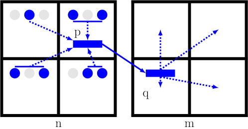
Figure 6: The various arrows exemplify the process of communicating data from each process on node $n$ to processes on node $m$ through a three-step algorithm. The bold circles on node $n$ represent vector values that must be communicated to node $m$.

This figure displays a portion of a parallel system consisting of 8 processes partitioned across two nodes, labeled $n$ and $m$. The solid circles on node $n$ represent vector values that must be sent to node $m$. Therefore, each process on node $n$ must send values to processes on node $m$. Instead of sending directly to destination processes, each process $(s,n)$ sends to the process labeled $(p,n)$, displayed by the dashed arrows on node $n$. Process $(p,n)$ then sends all collected values through the network to process $(q,m)$. Finally, process $(q,m)$ distributes received values among the processes local to node $m$, displayed by the dashed arrows on node $m$.

On-node data is communicated directly between the process on which the vector values are stored and that which requires the data, as displayed in Figure 7.

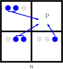
Figure 7: An example of how vector values corresponding with matrix entries in the on-node block are communicated. All values $(p,n)$ must receive from other processes $(q,n)$ are communicated directly as nothing is injected into the network.

In this example, the solid circles represent vector values that are stored on each process $(s,n)$ and needed by $(p,n)$. This data is sent directly between the processes in a single step.

4.1 Inter-node communication setup

To eliminate the communication of duplicated messages, a list of communicating nodes is formed for each node $n$ along with the accompanying data values. These lists are then distributed across all processes local to $n$ by balancing the number of nodes and volume of data for communication. To facilitate this, the function $\mathcal{N}(n)$ defines the set of nodes to which the processes on node $n$ must send,

$$\begin{split}\mathcal{N}(n)&=\left\{m\,\middle|\,\textnormal{$\exists$ $p$, $q$ s.t. $A_{ij}\neq\ 0$}\right.\\ &\left.\textnormal{with $i\in\ \mathcal{R}{((q,m))}$, $j\in\ \mathcal{R}{((p,n))}$, $n\neq\ m$}\vphantom{m}\right\}.\end{split}$$ (13)

Table 5 contains $\mathcal{N}(n)$, the list of nodes to which each node $n$ sends.

	$n$
	0	1	2
$\mathcal{N}(n)$	$\left\{1,2\right\}$	$\left\{0,2\right\}$	$\left\{0\right\}$

Table 5: Communication requirements for each node $n$ in Example 2.1.

The associated data values are defined for each node $m\in\mathcal{N}(n)$ with $\mathcal{E}(n,m)$, which returns the data indices to be sent from node $n$ to node $m$. That is,

$$\mathcal{E}(n,m)=\left\{i\,|\,\exists\ \textnormal{$p$, $q$ s.t. $A_{ij}\neq\ 0$ with $i\in\mathcal{R}{((q,m))}$}\right.,\\ \left.\textnormal{$j\in\mathcal{R}{((p,n))}$, $n\neq\ m$}\right\}.$$ (14)

Extending Example 2.1, Table 6 displays the global vector indices, $\mathcal{E}(n,m)$, for each set of nodes $n$ and $m$.

		$n$
		0	1	2
$m$	0	$\left\{\right\}$	$\left\{3\right\}$	$\left\{4,5\right\}$
	1	$\left\{0,1\right\}$	$\left\{\right\}$	$\left\{\right\}$
	2	$\left\{0\right\}$	$\left\{2\right\}$	$\left\{\right\}$

Table 6: In Example 2.1, each column $n$ contains the values sent from $n$ to $m$, as in $\mathcal{E}(n,m)$.

$\mathcal{T}((p,n))$ defines the nodes to which $(p,n)$ must send, that is the nodes in $\mathcal{N}(n)$ that are distributed to process $(p,n)$. Similarly, $\mathcal{U}((p,n))$ contains the nodes that send to $(p,n)$. Specifically,

$$\mathcal{T}((p,n)) =\left\{m\in\mathcal{N}(n)\,\middle|\,m\;\textnormal{maps to}\;(p,n)\right\},$$ (15)

$$\mathcal{U}((p,n)) =\left\{m\,\middle|\,n\in\mathcal{N}(m),\ n\;\textnormal{maps to}\;(p,n)\right\}.$$ (16)

This paper considers a simple distribution in which the node $m\in\mathcal{N}(n)$ to which the most data $\left|\mathcal{D}(n,m)\right|$ is sent is mapped to process $(0,n)$, the node with the second most data is mapped to process $(1,n)$, and so on. The opposite ordering is used for $\mathcal{U}((p,n))$, mapping the node $n\in\mathcal{N}(m)$ with largest $\left|\mathcal{D}(m,n)\right|$ to process $(\textnormal{{ppn}}-1,n)$, the second largest to process $(\textnormal{{ppn}}-2,n)$, etc. If there are fewer nodes in $\mathcal{N}(n)$ than there are processes per node, a single node is mapped to multiple local processes so that all processes communicate. There are various other possible mapping strategies, such as mapping a node $m$ to the process $(p,n)$ storing the majority of the data in $\mathcal{D}(n,m)$. However, as this would only affect intra-node communication requirements, these mappings are not explored in this paper.

The processor layout in Example 2.1 is displayed in Table 7, where the columns contain the send and receive nodes that are mapped to each process.

	$(p,n)$
	(0, 0)	(1, 0)	(0, 1)	(1, 1)	(0, 2)	(1, 2)
$\mathcal{T}((p,n))$	$\left\{1\right\}$	$\left\{2\right\}$	$\left\{0\right\}$	$\left\{2\right\}$	$\left\{0\right\}$	$\left\{\right\}$
$\mathcal{U}((p,n))$	$\left\{2\right\}$	$\left\{1\right\}$	$\left\{\right\}$	$\left\{0\right\}$	$\left\{1\right\}$	$\left\{0\right\}$

Table 7: Processor mappings for $\mathcal{N}(n)$, namely $\mathcal{T}((p,n))$ and $\mathcal{U}((p,n))$ for Example 2.1.

Finally, $\mathcal{G}((p,n))$ defines the set of all off-node processes to which process $(p,n)$ sends data during the inter-node communication step of the NAPSpMV. Specifically,

$$\mathcal{G}((p,n)) =\left\{(q,m)\,\middle|\,m\in\mathcal{T}((p,n)),\,n\in\mathcal{U}((q,m))\right\}.$$ (17)

Following Example 2.1, the columns of Table 8 list the indices of the values that each $(p,n)$ sends, $\mathcal{G}((p,n))$.

	$(p,n)$
	(0, 0)	(1, 0)	(0, 1)	(1, 1)	(0, 2)	(1, 2)
$\mathcal{G}((p,n))$	$\left\{(1,1)\right\}$	$\left\{(1,2)\right\}$	$\left\{(1,0)\right\}$	$\left\{(0,2)\right\}$	$\left\{(0,0)\right\}$	$\left\{\right\}$

Table 8: Inter-node communication requirements of each process $(p,n)$ for Example 2.1

.

Finally, let $\mathcal{I}((p,n),(q,m))$ define the global data indices corresponding to the values sent from process $(p,n)$ to $(q,m)$:

$$\mathcal{I}((p,n),(q,m))=\\ \left\{\mathcal{E}(n,m)\,\middle|\,m\in\mathcal{T}((p,n)),\,n\in\mathcal{U}((q,m)\right\}$$ (18)

The global vector indices to which each process $(p,n)$ sends and receives for Example 2.1 are displayed in Table 9.

	$(p,n)$
		(0, 0)	(1, 0)	(0, 1)	(1, 1)	(0, 2)	(1, 2)
$(q,m)$	(0, 0)	$\left\{\right\}$	$\left\{\right\}$	$\left\{\right\}$	$\left\{\right\}$	$\left\{4,5\right\}$	$\left\{\right\}$
	(1, 0)	$\left\{\right\}$	$\left\{\right\}$	$\left\{3\right\}$	$\left\{\right\}$	$\left\{\right\}$	$\left\{\right\}$
	(0, 1)	$\left\{\right\}$	$\left\{\right\}$	$\left\{\right\}$	$\left\{\right\}$	$\left\{\right\}$	$\left\{\right\}$
	(1, 1)	$\left\{0\right\}$	$\left\{\right\}$	$\left\{\right\}$	$\left\{\right\}$	$\left\{\right\}$	$\left\{\right\}$
	(0, 2)	$\left\{\right\}$	$\left\{\right\}$	$\left\{\right\}$	$\left\{2\right\}$	$\left\{\right\}$	$\left\{\right\}$
	(1, 2)	$\left\{\right\}$	$\left\{0,1\right\}$	$\left\{\right\}$	$\left\{\right\}$	$\left\{\right\}$	$\left\{\right\}$

Table 9: Inter-node communication requirements for each set of processes $(p,n)$ and $(q,m)$. Each column $(p,n)$ contains the indices of values sent from $(p,n)$ to $(q,m)$.

4.2 Local Communication

The function $\mathcal{G}_{\text{send}}((p,n))$ for $p=0,\ldots,\textnormal{{ppn}}-1$, describes evenly distributed inter-node communication requirements for all processes local to node $n$. However, many of the vector indices to be sent to off-node process $(q,m)\in\mathcal{D}((p,n),(q,m))$, are not stored on process $(p,n)$. For instance, in Table 9, process $(0,1)$ sends global vector indices $0$ and $1$. However, only row $1$ is stored on process $(0,1)$, requiring vector component $0$ to be communicated before inter-node messages are sent.

Similarly, many of the indices that a process $(q,m)$ receives from $(p,n)$ are redistributed to various processes on node $n$. Table 9 requires process $(1,2)$ to receive vector data according to indices $0$ and $1$. Process $(0,2)$ uses both of these vector values, yielding a requirement for redistribution of data received from inter-node communication. Therefore, local communication requirements must be defined.

Each NAPSpMV consists of multiple steps of intra-node communication. Let a function $\mathcal{L}((p,n),\textnormal{{locality}})$ define all processes, local to node $n$, to which process $(p,n)$ sends messages, where locality is a tuple describing the locality of both the original location of the data as well as its final destination. The locality of each position is described as either on_node, meaning a process local to node $n$, or off_node, meaning a process local to node $m\neq n$.

There are three possible combinations for locality: 1. the data is initialized on_node with a final destination off_node; 2. the original data is off_node while the final destination is on_node; or 3. both the original data and the final location are on_node. These three types of intra-node communication are described in more detail in the remainder of Section 4.2.

For each process $(s,n)\in\mathcal{L}((p,n),\textnormal{{locality}})$, $\mathcal{J}((p,n),(s,n),\textnormal{{locality}})$ defines the global vector indices to be sent from process $(p,n)$ to $(s,n)$ through intra-node communication. This notation is used in following sections.

4.2.1 Local redistribution of initial data

During inter-node communication, a process $(p,n)$ sends all vector values corresponding to the global indices in $\mathcal{I}((p,n),(q,m))$ to each process $(q,m)\in\mathcal{G}((p,n))$. The indices in $\mathcal{I}((p,n),(q,m))$ originate on node $n$, but not necessarily process $(p,n)$. Therefore, the initial vector values must be redistributed among all processes local to node $n$.

Let $\mathcal{L}((p,n),(\texttt{on\_node},\texttt{off\_node}))$ represent all processes, local to node $n$, to which $(p,n)$ sends initial vector values. This function is defined as

$$\mathcal{L}((p,n),(\texttt{on\_node},\texttt{off\_node}))=\\ \left\{(s,n)\,\middle|\,\exists\,j\in\mathcal{R}((p,n)),\ j\in\mathcal{I}((s,n),(q,m))\right\}.$$ (19)

The local processes to which each $(p,n)$ sends initial data in Example 2.1 are displayed in Table 10.

	$(p,n)$
	(0, 0)	(1, 0)	(0, 1)	(1, 1)	(0, 2)	(1, 2)
$\mathcal{L}$	$\left\{(1,0)\right\}$	$\left\{\right\}$	$\left\{(1,1)\right\}$	$\left\{(0,1)\right\}$	$\left\{\right\}$	$\left\{(0,2)\right\}$

Table 10: Initial intra-node communication requirements for each process $(p,n)$ in Example 2.1. The row of the table describes $\mathcal{L}((p,n),(\texttt{on\_node},\texttt{off\_node}))$.

Furthermore, the data global vector indices that must be sent from process $(p,n)$ to each $(s,n)\in\mathcal{L}((p,n),(\texttt{on\_node},\texttt{off\_node}))$ are defined as

$$\mathcal{J}((p,n),(s,n),(\texttt{on\_node},\texttt{off\_node}))=\\ \left\{i\,\middle|\,i\in\mathcal{R}((p,n)),\forall\,i\in\mathcal{G}((s,n))\right\}.$$ (20)

The global vector indices that each $(p,n)$ must send to other processes on node $n$ in Example 2.1 are displayed in Figure 11.

	$(p,n)$
		(0, 0)	(1, 0)	(0, 1)	(1, 1)	(0, 2)	(1, 2)
$(q,n)$	(0, 0)	$\left\{\right\}$	$\left\{\right\}$	—	—	—	—
	(1, 0)	$\left\{0\right\}$	$\left\{\right\}$	—	—	—	—
	(0, 1)	—	—	$\left\{\right\}$	$\left\{3\right\}$	—	—
	(1, 1)	—	—	$\left\{2\right\}$	$\left\{\right\}$	—	—
	(0, 2)	—	—	—	—	$\left\{\right\}$	$\left\{5\right\}$
	(1, 2)	—	—	—	—	$\left\{\right\}$	$\left\{\right\}$

Table 11: Global vector indices of initial data that is communicated between processes local to each node $n$ in Example 2.1. Each column contains the indices of values sent from $(p,n)$ to $(q,n)$. Note: dashes (—) throughout the table represent processes on separate nodes, which do not communicate during intra-node communication.

4.2.2 Local redistribution of received off-node data

During inter-node communication, a process $(p,n)$ sends all data with final destination on node $m$ to process $(q,m)\in\mathcal{G}((p,n))$. Process $(q,m)$ then distributes these values across the processes local to node $m$. Let $\mathcal{L}((q,m),(\texttt{off\_node},\texttt{on\_node}))$ define all processes local to node $m$ to which process $(q,m)$ sends vector values that have been received through inter-node communication. This function is defined as

$$\mathcal{L}((q,m),(\texttt{off\_node},\texttt{on\_node}))=\\ \left\{(s,m)\,\middle|\,\exists\,A_{ij}\neq 0\;\textnormal{with}\;i\in\mathcal{R}((s,m)),\right.\\ \left.j\in\mathcal{I}((p,n),(q,m))\right\}.$$ (21)

This is highlighted, for Example 2.1, in Table 12.

	$(p,n)$
	(0, 0)	(1, 0)	(0, 1)	(1, 1)	(0, 2)	(1, 2)
$\mathcal{L}$	$\left\{\right\}$	$\left\{(0,0)\right\}$	$\left\{\right\}$	$\left\{\right\}$	$\left\{\right\}$	$\left\{(0,2)\right\}$

Table 12: Intra-node communication requirements containing processes to which each $(p,n)$ sends received inter-node data, according to Example 2.1. The row of the table describes $\mathcal{L}((p,n),(\texttt{off\_node},\texttt{on\_node}))$.

Furthermore, the data global vector indices that must be sent from process $(q,m)$ to each $(s,m)\in\mathcal{L}((q,m),(\texttt{off\_node},\texttt{on\_node}))$ are defined as

$$\mathcal{J}((q,m),(s,m),(\texttt{off\_node},\texttt{on\_node}))=\\ \left\{j\in\mathcal{I}((p,n),(q,m))\,\middle|\,A_{ij}\neq 0\;\textnormal{with}\;i\in\mathcal{R}((s,m))\right\}.$$ (22)

The global vector indices, received from the inter-node communication step, which $(p,n)$ must send to each local process $(q,n)$ in Example 2.1 are displayed in Table 13.

	$(p,n)$
		(0, 0)	(1, 0)	(0, 1)	(1, 1)	(0, 2)	(1, 2)
$(q,n)$	(0, 0)	$\left\{\right\}$	$\left\{3\right\}$	—	—	—	—
	(1, 0)	$\left\{\right\}$	$\left\{\right\}$	—	—	—	—
	(0, 1)	—	—	$\left\{\right\}$	$\left\{\right\}$	—	—
	(1, 1)	—	—	$\left\{\right\}$	$\left\{\right\}$	—	—
	(0, 2)	—	—	—	—	$\left\{\right\}$	$\left\{1\right\}$
	(1, 2)	—	—	—	—	$\left\{\right\}$	$\left\{\right\}$

Table 13: Global vector indices of received inter-node data that must be communicated between processes local to each node $n$ in Example 2.1. Each column contains the indices of values sent from $(p,n)$ to $(q,n)$. Note: dashes (—) throughout the table represent processes on separate nodes, which cannot communicate during intra-node communication.

4.2.3 Fully Local Communication

A subset of the values needed by a process $(p,n)$ are stored on local process $(s,n)$. One advantage is that these values bypass the three-step communication, and are communicated directly. Let $\mathcal{L}((p,n),(\texttt{on\_node},\texttt{on\_node}))$ define all processes local to node $n$ to which $(p,n)$ sends vector data. This function is defined as

$$\mathcal{L}((p,n),(\texttt{on\_node},\texttt{on\_node}))=\\ \left\{(s,n)\,\middle|\,\exists\,A_{ij}\neq 0\;\textnormal{with}\;i\in\mathcal{R}((s,n)),j\in\mathcal{R}((p,n))\right\}.$$ (23)

The processes local to node $n$, to which $(p,n)$ must send initial vector data in Example 2.1 are displayed in Table 14.

	$(p,n)$
	(0, 0)	(1, 0)	(0, 1)	(1, 1)	(0, 2)	(1, 2)
$\mathcal{L}$	$\left\{\right\}$	$\left\{(0,0)\right\}$	$\left\{\right\}$	$\left\{(0,1)\right\}$	$\left\{\right\}$	$\left\{\right\}$

Table 14: Intra-node communication requirements containing processes to which each process $(p,n)$ must send vector data, according to Example 2.1. The row of the table describes $\mathcal{L}((p,n),(\texttt{on\_node},\texttt{on\_node}))$.

Furthermore, the global vector indices that must be sent from process $(p,n)$ to each $(s,n)\in\mathcal{L}((p,n),(\texttt{on\_node},\texttt{on\_node}))$ is defined as follows.

$$\mathcal{J}((p,n),(s,n),(\texttt{on\_node},\texttt{on\_node}))=\\ \left\{j\,\middle|\,\exists\,A_{ij}\neq 0\;\textnormal{with}\;i\in\mathcal{R}((s,n)),j\in\mathcal{R}((p,n))\right\}.$$ (24)

The global vector indices which $(p,n)$ must send to each local process $(s,n)$ in Example 2.1 are displayed in Table 15.

	$(p,n)$
		(0, 0)	(1, 0)	(0, 1)	(1, 1)	(0, 2)	(1, 2)
$(s,n)$	(0, 0)	$\left\{\right\}$	$\left\{1\right\}$	—	—	—	—
	(1, 0)	$\left\{\right\}$	$\left\{\right\}$	—	—	—	—
	(0, 1)	—	—	$\left\{\right\}$	$\left\{3\right\}$	—	—
	(1, 1)	—	—	$\left\{\right\}$	$\left\{\right\}$	—	—
	(0, 2)	—	—	—	—	$\left\{\right\}$	$\left\{\right\}$
	(1, 2)	—	—	—	—	$\left\{\right\}$	$\left\{\right\}$

Table 15: Global vector indices that must be communicated between processes local to each node $n$ in Example 2.1. Each column contains the indices of values sent from $(p,n)$ to $(q,n)$. Note: dashes (—) throughout the table represent processes on separate nodes, which cannot communicate during intra-node communication.

4.3 Alternative SpMV Algorithm

Input:

$(p,n)$ :	tuple describing local rank and
	node of process
$v|_{\mathcal{R}((p,n))}$:	rows of input vector $v$ local to
	process $(p,n)$
locality:	locality of input and output data

Output:

$\ell_{\text{recv}}$:	values that rank $(p,n)$ receives from
	other processes

// Initialize sends

for $(s,n)\in\mathcal{L}((p,n),\textnormal{{locality}})$ do

       for $i\in\mathcal{J}((p,n),(s,n),\textnormal{{locality}})$ do

             $\ell_{\text{send}}\leftarrow v|_{\mathcal{R}((p,n))_{i}}$

            

      ${\textnormal{{MPI\_Isend}}}(\ell_{\text{send}},\ldots,(s,n),\ldots)$

// Initialize receives

$\ell_{\text{recv}}\leftarrow\emptyset$

for $(s,n)$ s.t. $(p,n)\in\mathcal{L}((s,n),\textnormal{{locality}})$ do

       ${\textnormal{{MPI\_Irecv}}}(\ell_{\text{recv}},\ldots,(s,n),\ldots)$

// Complete sends and receives

MPI_Waitall

Algorithm 2 local_comm

The method of communicating vector values to on-node processes is described in Algorithm 2. Using the definitions for the various steps of intra- and inter-node communication, the NAPSpMV is described in Algorithm 3, where ${\textnormal{{local\_spmv}}}()$ refers to a row-wise, non-distributed SpMV — e.g. with Intel’s MKL library or with the Eigen Library. It is important to note that many slight variations to the algorithm are possible. The fully local communication has no dependencies, and can be performed anytime before calling ${\textnormal{{local\_spmv}}}(A_{\text{on\_node}},b_{\ell\rightarrow\ell})$. Furthermore, the function ${\textnormal{{local\_spmv}}}(A_{\text{on\_process}},v|\mathcal{R})$ has no communication requirements and, hence, can be performed at any point in the algorithm.

Input:

$(p,n)$:	tuple describing local rank and node
	of process
$A|R$:	rows of matrix $A$ local to process (p, n)
$v|R$:	rows of input vector $v$ local to process
	(p, n)

Output:

$w|\mathcal{R}$:	rows of output vector $w\leftarrow Av$,
	local to process $(p,n)$

$A_{\text{on\_process}}=\texttt{on\_process}(A|\mathcal{R})$

$A_{\text{on\_node}}=\texttt{on\_node}(A|\mathcal{R})$

$A_{\text{off\_node}}=\texttt{off\_node}(A|\mathcal{R})$

$b_{\ell\rightarrow\ell}\leftarrow{\textnormal{{local\_comm}}}((p,n),v|\mathcal{R},(\texttt{on\_node}\rightarrow\texttt{on\_node}))$

$b_{\ell\rightarrow n\ell}\leftarrow{\textnormal{{local\_comm}}}((p,n),v|\mathcal{R},(\texttt{on\_node}\rightarrow\texttt{off\_node}))$

// Initialize sends

for $(q,m)\in\mathcal{G}((p,n))$ do

       for $i\in\mathcal{I}((p,n),(q,m))$ do

             $g_{\text{send}}\leftarrow b_{\ell\rightarrow n\ell}^{i}$

            

      ${\textnormal{{MPI\_Isend}}}(g_{\text{send}},\ldots,(q,m),\ldots)$

// Initialize receives

$g_{\text{recv}}\leftarrow\emptyset$

for $(q,m)$ s.t. $(p,n)\in\mathcal{G}((q,m))$ do

       ${\textnormal{{MPI\_Irecv}}}(g_{\text{recv}},\ldots,(q,m),\ldots)$

// Serial SpMV for local values

${\textnormal{{local\_spmv}}}(A_{\text{on\_process}},v|\mathcal{R})$

// Serial SpMv for on-node values

${\textnormal{{local\_spmv}}}(A_{\text{on\_node}},b_{\ell\rightarrow\ell})$

// Complete sends and receives

MPI_Waitall

$b_{n\ell\rightarrow\ell}\leftarrow{\textnormal{{local\_comm}}}((p,n),v|\mathcal{R},(\texttt{off\_node}\rightarrow\texttt{on\_node}))$

// Serial SpMV for off-node values

${\textnormal{{local\_spmv}}}(A_{\text{off\_node}},b_{n\ell\rightarrow\ell})$

Algorithm 3 NAPSpMV

5 Results

In this section, the parallel performance and scalability of the NAPSpMV in comparison to the standard SpMV is presented. The matrix-vector multiplication in an algebraic multigrid (AMG) hierarchy is tested for both a structured 2D rotated anisotropic and for unstructured linear elasticity on $32\,768$ processes in order to expose a variety of communication patterns. In addition, scaling tests are considered for random matrices with a constant number of non-zeros per row to investigate problems with no structure. Lastly, scaling tests on the largest 15 matrices from the SuiteSparse matrix collection are presented. All tests are performed on the Blue Waters parallel computer at University of Illinois at Urbana-Champaign.

AMG hierarchies consist of successively coarser, but denser levels. Therefore, while a standard SpMV performed on the original matrix often requires communication of a small number of large messages, coarse levels require a large number of small messages to be injected into the network. Figure 8 shows that both the number and size of inter-node messages required on each level of the linear elasticity hierarchy are reduced through use of the NAPSpMV. There is a large reduction in communication requirements for coarse levels of the hierarchy, which includes a high number of small messages. However, as the NAPSpMV requires redistribution of data among processes local to each node, the intra-node communication requirements increase greatly for the NAPSpMV, as shown in Figure 9.

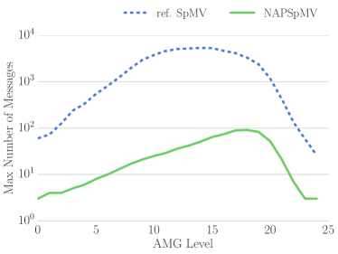
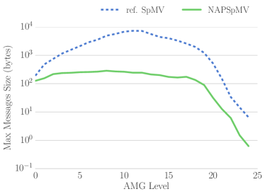
Figure 8: The maximum number (top) and size (bottom) of inter-node messages communicated by a single process during a standard SpMV and NAPSpMV on each level of the linear elasticity AMG hierarchy.

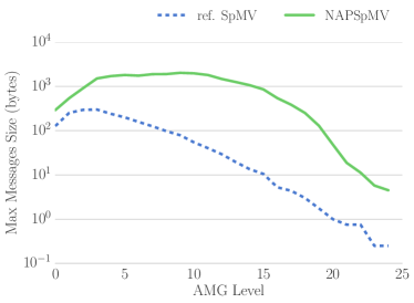
Figure 9: The maximum number (top) and size (bottom) of intra-node messages communicated by a single process during a standard SpMV and NAPSpMV on each level of the linear elasticity AMG hierarchy.

While there is an increase in intra-node communication requirements, the reduction in more expensive inter-node messages results in a significant reduction in total time for the NAPSpMV algorithm, particularly on coarser levels near the middle of each AMG hierarchy, as shown in Figure 10.

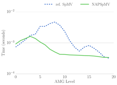
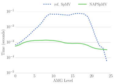
Figure 10: The time required to perform the various SpMVs on each level of the rotated anisotropic (left) and linear elasticity (right) AMG hierarchies.

Random matrices, formed with a constant number of non-zeros per row, lack structure that is found in many finite element discretizations. As these matrices are distributed across an increasingly large number of processes, non-zeros are more likely to be located in off-process blocks of the matrix. Therefore, both weak and strong scaling studies of random matrices yield increases in communication requirements with scale.The sparsity pattern of random matrices varies with random number generator seeds and are dependent on the number of non-zeros per row. Therefore, the standard SpMV and NAPSpMV were performed on five different random matrices for each tested density of $25$, $50$, and $100$ non-zeros per row, as shown in Figure 11.

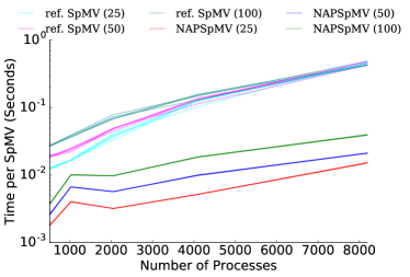
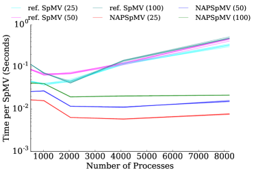
Figure 11: The time required to perform the various SpMVs on weakly (left) and strongly (right) scaled random matrices. Five different random matrices are tested for each density of $25$, $50$, and $100$ non-zeros per row. The weak-scaling study tests matrices with $1\,000$ rows per process, while the strongly-scaled matrix contains $4\,096\,000$ rows.

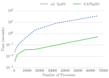
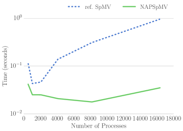
Figure 12: The time required to perform the various SpMVs on weakly (left) and strongly (right) scaled random matrices, each with $100$ non-zeros per row. The weak-scaling study tests matrices with $1\,000$ rows per process, while the strongly-scaled matrix contains $4\,096\,000$ rows.

The standard and NAPSpMV costs for all random matrices of equivalent density are comparable. Furthermore, there is little difference in costs between each density. Therefore, extended tests are performed on only a single random matrix with $100$ non-zeros per row. Figure 12 displays the time required for a NAPSpMV in comparison to the standard SpMV in both weak and strong scaling studies. For these random matrices, the NAPSpMV exhibits improved performance over the reference implementation by up to two orders of magnitude and also improves scalability.

The time required to perform the various SpMVs on $13$ of the $15$ largest matrices from the SuiteSparse matrix collection are shown with strided and balanced partitions, in Figures 13 and 14 respectively. The remaining $2$ large matrices were not included due to partitioning constraints.

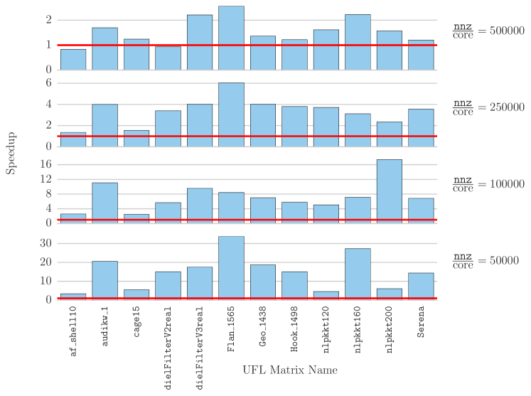
Figure 13: The speedup of NAPSpMVs over reference SpMVs on a subset of the largest real matrices from the SuiteSparse matrix collection at various scales, where $\frac{nnz}{\textnormal{core}}$ is the average number of non-zeros per core, partitioned so that each row $r$ is stored on process $p=r\mod n_{p}$, where $n_{p}$ is the number of processes.

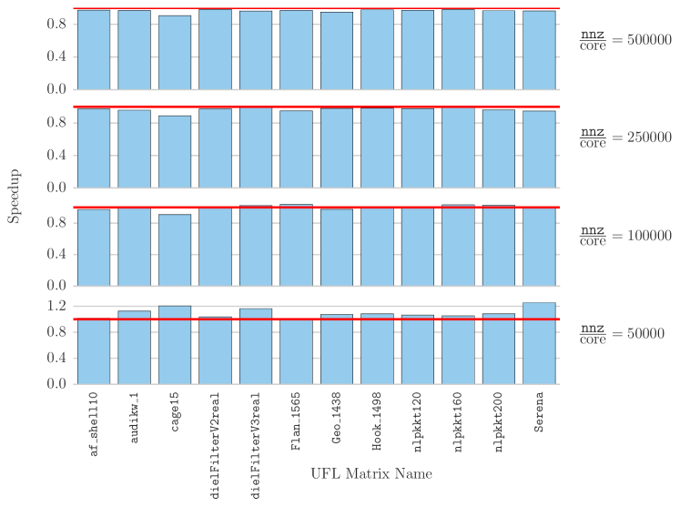
Figure 14: The speedup of NAPSpMVs over reference SpMVs on a subset of the largest real matrices from the SuiteSparse matrix collection at various scales, where $\frac{nnz}{\textnormal{core}}$ is the average number of non-zeros per core, partitioned with PT Scotch.

For the strided partitions with $n_{p}$ processes, each row $r$ is local to process $p=r\mod n_{p}$. As some matrices in this subset have nearly dense blocks of rows, this allows for improved load balancing over each process holding a contiguous block of rows. The balanced partitions were formed with PT Scotch graph partitioning, using the strategy SCOTCH_STRATBALANCE.

The NAPSpMV improves upon many of the matrices with strided partitions, as communication patterns are far from optimal, while only minimally improving upon the graph partitioned matrices. However, the cost of partitioning motivates the use of less optimal partitions when a smaller number of SpMVs are to be performed. Figure 15 shows the time required to perform various numbers of NAPSpMVs on both the strided and balanced partitions at the strongest scale tested, with $50\,000$ non-zeros per core.

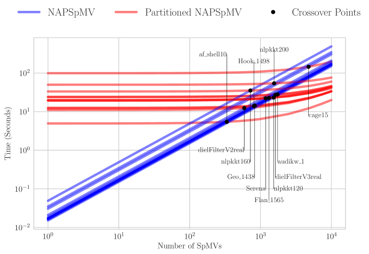
Figure 15: The time required to perform various numbers of NAPSpMVs on strided and balanced partitions of the largest real SuiteSparse matrices with $50\,000$ non-zeros per process. The time to perform a NAPSpMV on a balanced partition includes the setup cost of partitioning and redistributing the matrix. The crossover points represent the number of NAPSpMVs required before graph partitioning becomes less costly than performing NAPSpMVs on the strided partition.

In these tests, the balanced partitioned timings include the time required to graph partition and redistribute the matrix. The crossover point for the various SuiteSparse matrices, at which the graph partitioning becomes less costly than performing NAPSpMVs on strided partitions, occurs only after hundreds, or often thousands, of SpMVs have been performed.

6 Conclusion and Future Work

This paper introduces a method to reduce communication that is injected into the network during a sparse matrix-vector multiply by reorganizing messages on each node. This results in a reduction of the inter-node communication, replaced by less-costly intra-node communication, which reduces both the number and size of messages that are injected into the network. The current implementation could be extended to take various levels of the hierarchy into account, such as splitting intra-node messages into on-socket and off-socket. Figure 16 shows that on-socket messages are significantly cheaper and could be targeted to further reduce communication costs.

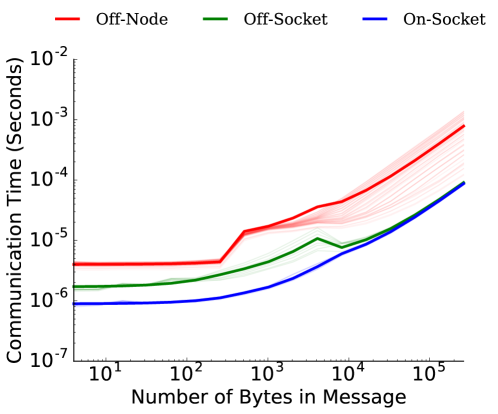
Figure 16: The time required to send a single message of various sizes, with the thin lines representing timings measured by Nodecomm and the thick lines displaying the max-rate and intra-node models in (10) and (12), respectively. The intra-node models are split into two categories, on-socket and off-socket.

References

-
[1]
T. A. Davis, Y. Hu, The
university of florida sparse matrix collection, ACM Transactions on
Mathematical Software 32 (2011) 1:1 – 1:25.
URL http://www.cise.ufl.edu/research/sparse/matrices -
[2]
S. Williams, L. Oliker, R. Vuduc, J. Shalf, K. Yelick, J. Demmel,
Optimization of sparse
matrix-vector multiplication on emerging multicore platforms, in:
Proceedings of the 2007 ACM/IEEE Conference on Supercomputing, SC ’07, ACM,
New York, NY, USA, 2007, pp. 38:1–38:12.
doi:10.1145/1362622.1362674.
URL http://doi.acm.org/10.1145/1362622.1362674 -
[3]
W. Gropp, L. N. Olson, P. Samfass,
Modeling MPI
communication performance on SMP nodes: Is it time to retire the ping pong
test, in: Proceedings of the 23rd European MPI Users’ Group Meeting, EuroMPI
2016, ACM, New York, NY, USA, 2016, pp. 41–50.
doi:10.1145/2966884.2966919.
URL http://doi.acm.org/10.1145/2966884.2966919 -
[4]
A. Pinar, C. Aykanat, Fast
optimal load balancing algorithms for 1d partitioning, J. Parallel Distrib.
Comput. 64 (8) (2004) 974–996.
doi:10.1016/j.jpdc.2004.05.003.
URL http://dx.doi.org/10.1016/j.jpdc.2004.05.003 -
[5]
B. Hendrickson, T. G. Kolda,
Graph partitioning
models for parallel computing, Parallel Comput. 26 (12) (2000) 1519–1534.
doi:10.1016/S0167-8191(00)00048-X.
URL http://dx.doi.org/10.1016/S0167-8191(00)00048-X -
[6]
B. Vastenhouw, R. H. Bisseling,
A two-dimensional data
distribution method for parallel sparse matrix-vector multiplication, SIAM
Review 47 (1) (2005) 67–95.
arXiv:https://doi.org/10.1137/S0036144502409019, doi:10.1137/S0036144502409019.
URL https://doi.org/10.1137/S0036144502409019 -
[7]
Ümi̇t V. Çatalyürek, C. Aykanat, B. Uçar,
On two-dimensional sparse matrix
partitioning: Models, methods, and a recipe, SIAM Journal on Scientific
Computing 32 (2) (2010) 656–683.
arXiv:https://doi.org/10.1137/080737770, doi:10.1137/080737770.
URL https://doi.org/10.1137/080737770 -
[8]
G. Karypis, V. Kumar, A
parallel algorithm for multilevel graph partitioning and sparse matrix
ordering, J. Parallel Distrib. Comput. 48 (1) (1998) 71–95.
doi:10.1006/jpdc.1997.1403.
URL http://dx.doi.org/10.1006/jpdc.1997.1403 -
[9]
C. Chevalier, F. Pellegrini,
PT-Scotch:
A tool for efficient parallel graph ordering, Parallel Computing 34 (6–8)
(2008) 318 – 331, parallel Matrix Algorithms and Applications.
doi:http://dx.doi.org/10.1016/j.parco.2007.12.001.
URL http://www.sciencedirect.com/science/article/pii/S0167819107001342 - [10] U. V. Çatalyürek, C. Aykanat, Hypergraph-partitioning-based decomposition for parallel sparse-matrix vector multiplication, IEEE Transactions on Parallel and Distributed Systems 10 (7) (1999) 673–693. doi:10.1109/71.780863.
- [11] E. Jeannot, E. Meneses, G. Mercier, F. Tessier, G. Zheng, Communication and topology-aware load balancing in charm++ with treematch, in: 2013 IEEE International Conference on Cluster Computing (CLUSTER), 2013, pp. 1–8. doi:10.1109/CLUSTER.2013.6702666.
-
[12]
T. Agarwal, A. Sharma, L. V. Kalé,
Topology-aware task
mapping for reducing communication contention on large parallel machines,
in: Proceedings of the 20th International Conference on Parallel and
Distributed Processing, IPDPS’06, IEEE Computer Society, Washington, DC, USA,
2006, pp. 145–145.
URL http://dl.acm.org/citation.cfm?id=1898953.1899075 -
[13]
S. Sreepathi, E. D’Azevedo, B. Philip, P. Worley,
Communication
characterization and optimization of applications using topology-aware task
mapping on large supercomputers, in: Proceedings of the 7th ACM/SPEC on
International Conference on Performance Engineering, ICPE ’16, ACM, New York,
NY, USA, 2016, pp. 225–236.
doi:10.1145/2851553.2851575.
URL http://doi.acm.org/10.1145/2851553.2851575 -
[14]
T. Malik, V. Rychkov, A. Lastovetsky,
Network-aware optimization of
communications for parallel matrix multiplication on hierarchical hpc
platforms, Concurr. Comput. : Pract. Exper. 28 (3) (2016) 802–821.
doi:10.1002/cpe.3609.
URL http://dx.doi.org/10.1002/cpe.3609 -
[15]
J. L. Träff,
Implementing the mpi
process topology mechanism, in: Proceedings of the 2002 ACM/IEEE Conference
on Supercomputing, SC ’02, IEEE Computer Society Press, Los Alamitos, CA,
USA, 2002, pp. 1–14.
URL http://dl.acm.org/citation.cfm?id=762761.762767 -
[16]
E. Solomonik, A. Bhatele, J. Demmel,
Improving communication
performance in dense linear algebra via topology aware collectives, in:
Proceedings of 2011 International Conference for High Performance Computing,
Networking, Storage and Analysis, SC ’11, ACM, New York, NY, USA, 2011, pp.
77:1–77:11.
doi:10.1145/2063384.2063487.
URL http://doi.acm.org/10.1145/2063384.2063487 -
[17]
T. Kielmann, R. F. H. Hofman, H. E. Bal, A. Plaat, R. A. F. Bhoedjang,
Magpie: Mpi’s collective
communication operations for clustered wide area systems, SIGPLAN Not.
34 (8) (1999) 131–140.
doi:10.1145/329366.301116.
URL http://doi.acm.org/10.1145/329366.301116 - [18] N. T. Karonis, B. R. de Supinski, I. Foster, W. Gropp, E. Lusk, J. Bresnahan, Exploiting hierarchy in parallel computer networks to optimize collective operation performance, in: Proceedings 14th International Parallel and Distributed Processing Symposium. IPDPS 2000, 2000, pp. 377–384. doi:10.1109/IPDPS.2000.846009.
-
[19]
P. Sack, W. Gropp, Faster
topology-aware collective algorithms through non-minimal communication, in:
Proceedings of the 17th ACM SIGPLAN Symposium on Principles and Practice of
Parallel Programming, PPoPP ’12, ACM, New York, NY, USA, 2012, pp. 45–54.
doi:10.1145/2145816.2145823.
URL http://doi.acm.org/10.1145/2145816.2145823 - [20] L. Wesolowski, R. Venkataraman, A. Gupta, J. S. Yeom, K. Bisset, Y. Sun, P. Jetley, T. R. Quinn, L. V. Kale, Tram: Optimizing fine-grained communication with topological routing and aggregation of messages, in: 2014 43rd International Conference on Parallel Processing, 2014, pp. 211–220. doi:10.1109/ICPP.2014.30.
- [21] N. Bell, M. Garland, Efficient sparse matrix-vector multiplication on CUDA, NVIDIA Technical Report NVR-2008-004, NVIDIA Corporation (Dec. 2008).
-
[22]
S. Dalton, L. Olson, N. Bell,
Optimizing sparse
matrix—matrix multiplication for the gpu, ACM Trans. Math. Softw.
41 (4) (2015) 25:1–25:20.
doi:10.1145/2699470.
URL http://doi.acm.org/10.1145/2699470 -
[23]
H. D. Sterck, U. M. Yang, J. J. Heys,
Reducing complexity in parallel
algebraic multigrid preconditioners, SIAM Journal on Matrix Analysis and
Applications 27 (4) (2006) 1019–1039.
arXiv:https://doi.org/10.1137/040615729, doi:10.1137/040615729.
URL https://doi.org/10.1137/040615729 -
[24]
A. Bienz, R. D. Falgout, W. Gropp, L. N. Olson, J. B. Schroder,
Reducing parallel communication in
algebraic multigrid through sparsification, SIAM Journal on Scientific
Computing 38 (5) (2016) S332–S357.
arXiv:https://doi.org/10.1137/15M1026341, doi:10.1137/15M1026341.
URL https://doi.org/10.1137/15M1026341 -
[25]
N. Bell, S. Dalton, L. N. Olson,
Exposing fine-grained parallelism in
algebraic multigrid methods, SIAM Journal on Scientific Computing 34 (4)
(2012) C123–C152.
arXiv:https://doi.org/10.1137/110838844, doi:10.1137/110838844.
URL https://doi.org/10.1137/110838844 -
[26]
R. H. Bisseling, W. Meesen, Communication
balancing in parallel sparse matrix-vector multiplication., ETNA. Electronic
Transactions on Numerical Analysis [electronic only] 21 (2005) 47–65.
URL http://eudml.org/doc/128024 -
[27]
G. Schubert, H. Fehske, G. Hager, G. Wellein,
Hybrid-parallel
sparse matrix-vector multiplication with explicit communication overlap on
current multicore-based systems, Parallel Processing Letters 21 (03) (2011)
339–358.
arXiv:http://www.worldscientific.com/doi/pdf/10.1142/S0129626411000254,
doi:10.1142/S0129626411000254.
URL http://www.worldscientific.com/doi/abs/10.1142/S0129626411000254 -
[28]
R. Geus, S. Röllin,
Towards
a fast parallel sparse symmetric matrix–vector multiplication, Parallel
Computing 27 (7) (2001) 883 – 896, linear systems and associated problems.
doi:http://dx.doi.org/10.1016/S0167-8191(01)00073-4.
URL //www.sciencedirect.com/science/article/pii/S0167819101000734