Fermion confinement via Quantum Walks in 2D+1 and 3D+1 spacetime

Abstract

We analyze the properties of a two and three dimensional quantum walk that are inspired by the idea of a brane-world model put forward by Rubakov and Shaposhnikov Rubakov and Shaposhnikov (1983). In that model, particles are dynamically confined on the brane due to the interaction with a scalar field. We translated this model into an alternate quantum walk with a coin that depends on the external field, with a dependence which mimics a domain wall solution. As in the original model, fermions (in our case, the walker), become localized in one of the dimensions, not from the action of a random noise on the lattice (as in the case of Anderson localization), but from a regular dependence in space. On the other hand, the resulting quantum walk can move freely along the “ordinary” dimensions.

I Introduction

The quantum walk (QW) is the quantum analogue of the classical random walk. As in the case of random walks, QWs can appear either under its discrete-time Y. Aharonov, L. Davidovich (1993) or continuous-time Farhi and Gutmann (1998) form. We will concentrate here on discrete-time QWs, first considered by Grössing and Zeilinger Grossing and Zeilinger (1988) in 1988, as simple one-particle quantum cellular automata, and later popularized in the physics community in 1993, by Y. Aharonov Y. Aharonov, L. Davidovich (1993). The dynamics of such QWs consists on a quantum particle taking steps on a lattice conditioned on its internal state, typically a (pseudo) spin one half system. The particle dynamically explores a large Hilbert space associated with the positions of the lattice and allows thus to simulate a wide range of transport phenomena Kempe (2003). With QWs, the transport is driven by an external discrete unitary operation, which sets it apart from other lattice quantum simulation concepts where transport typically rests on tunneling between adjacent sites Bloch et al. (2012): all dynamic processes are discrete in space and time. It has been shown that any quantum algorithm can be recast under the form of a QW on a certain graph: QWs can be used for universal quantum computation, this being provable for both the continuous Childs (2009) and the discrete version Lovett et al. (2010). As models of coherent quantum transport, they are interesting both for fundamental quantum physics and for applications. An important field of applications is quantum algorithmic Ambainis (2003). QWs were first conceived as a natural tool to explore graphs, for example for efficient data searching (see e.g. Magniez et al. (2011)). They are also useful in condensed matter applications and topological phases Kitagawa et al. (2012). A totally new emergent point of view concerning QWs concerns quantum simulation of gauge fields and high-energy physical laws Arnault et al. (2016); Genske et al. (2013); Molfetta and Pérez (2016). It is important to note that QWs can be realized experimentally with a wide range of physical objects and setups, for example as transport of photons in optical networks or optical fibers Schreiber et al. (2012), or atoms in optical lattices Côté et al. (2006).

Within the context of diffusion processes in lattices, spatial localization appears as a natural phenomenon. It can result from random noise on the lattice sites, giving rise to Anderson localization Anderson (1956), but it can also be driven by the action of an external periodic potential (see e.g. Aubry and André (1980); Grempel et al. (1982); Lahini et al. (2009)). Similarly, one obtains localization for the 1-dimensional QW when spatial disorder is included Joye and Merkli (2010); Schreiber et al. (2011); Crespi et al. (2013), via non-linear effects Navarrete-Benlloch et al. (2007), or using a spatially periodic coin Shikano and Katsura (2010). For higher dimensions, localization may appear, even in the noiseless case, from the choice of the coin operator Inui et al. (2004).

In this paper, we will propose a different variant of the QW that gives rise to localization, by introducing a site-dependent non-periodic coin operator. The model is inspired on a brane-world proposal with extra dimensions Rubakov and Shaposhnikov (1983), where particles are confined to live in the ordinary 3+1 dimensions by the action of a potential well created by some additional scalar field. In its simplest form, one accounts for massless fermions which are confined in the brane. This idea can be translated to describe a QW where the potential well manifests as a position-dependent coin operator. Differently to the situations described above, the confining field is not random nor periodic, being instead a monotonous function of the position. As we show, this kind of QW produces a dynamical localization of the QW as in the original model. In fact, it can be shown that, in the continuous space-time limit, one reproduces the dynamics of a massless Dirac fermion. In this way, we establish an interesting parallelism between a high-energy quantum field theory, and a QW model that results in localization.

The rest of this paper is organized as follows. In Sect. II we briefly introduce the original brane model Rubakov and Shaposhnikov (1983) that motivated our work. In Sect. III we make use of this model to introduce a QW on two dimensions with a position-dependent coin that simulates the domain wall “scalar field” along the second (or “extra dimension”). We show that this QW in fact results in a confinement of the walker, and that the space-time continuous limit indeed reproduces the dynamics of a Dirac particle coupled to the scalar field. These ideas are generalised to 3D in Sect. IV. Finally, Sect. V is devoted to summarizing and discussing our results.

II Domain wall model for particle physics

The possibility of extra dimensions of space was first suggested by Theodor Kaluza and Oscar Klein Kaluza (1921); Klein (1926) seeking for an unified theory of electromagnetic and gravitational fields into a higher dimensional field, with one of the dimensions compactified. However, experimental data from particle colliders restrict the compactification radius to such small scales that they become virtually impossible to access them experimentally. A way to overcome this difficulty Arkani-Hamed et al. (1999) makes use of the ideas put forward by Rubakov and Shaposhnikov Rubakov and Shaposhnikov (1983). In that paper, the authors propose a brane world scenario, in which space-time has (3+$N$)+1 dimensions, with ordinary (low energy) particles confined in a potential well which is narrow along $N$ spatial directions and flat along the remaining three directions. The origin of this potential well is suggested to have a dynamical origin. In the simplest case it can be created by an extra scalar field in $4+1$ dimensions, as described by the Lagrangian

$$\mathcal{L}=\frac{1}{2}\partial_{A}\partial^{A}\varphi-\frac{1}{2}m^{2}\varphi-\frac{1}{4}\lambda\varphi^{4},\,\,\,A=0,1,2,3,4,$$ (1)

with metrics $g_{AB}=(1,-1,-1,-1,-1)$. The classical equations of motion derived from the above Lagrangian admit a domain wall solution $\varphi(x^{4})$ that only depends on the coordinate $x^{4}$ along the extra dimension, and is given by

$$\varphi(x^{4})=\frac{m}{\sqrt{\lambda}}\tanh(\frac{mx^{4}}{\sqrt{2}}).$$ (2)

This model can account for left-handed massless fermions living in $3+1$ dimensions, if they are coupled to the scalar fields, as in the following Lagrangian:

$$\mathcal{L}_{\psi}=i\bar{\Psi}\Gamma^{A}\partial_{A}\Psi+h\varphi\bar{\Psi}\Psi,$$ (3)

where $h$ is the coupling constant, and the $4+1$-dimensional gamma matrices are $\Gamma^{\mu}=\gamma^{\mu}$, $\mu=0,\dots 3$, and $\Gamma^{4}=i\gamma^{5}$, with $\gamma^{\mu},\gamma^{5}$ the standard gamma matrices. From Eq. (3) the corresponding Dirac equation follows, which reads

$$i\Gamma^{A}\partial_{A}\Psi+h\varphi\Psi=0.$$ (4)

As discussed in Rubakov and Shaposhnikov (1983), this equation has a solution that is confined inside the domain wall, while the corresponding particles are left-handed massless fermions in the $3+1$ dimensional world. In the next Section, we make use of these ideas to introduce a QW model in $1+1+1$ dimensions that leads to confined fermions in $1+1$.

III 2D Quantum Walks inside a 1+1 Domain Wall

Consider a QW defined over discrete time and discrete two-dimensional space, with axis $x$, $y$. The discrete space points are labeled by $p$ and $q$, respectively, with $p,q\in\mathbb{Z}$, while time steps are labeled by $j\in\mathbb{N}$. This QW is driven by an in-homogeneous coin acting on the $2$-dimensional Hilbert space $\mathcal{H}_{\text{spin}}$. The evolution equations read

$$\begin{bmatrix}\psi_{j+1,p,q}^{\uparrow}\\ \psi_{j+1,p,q}^{\downarrow}\end{bmatrix}\ =S_{y}Q^{+}(\theta_{q})S_{x}Q^{-}(\theta_{q})\begin{bmatrix}\psi_{j,p,q}^{\uparrow}\\ \psi_{j,p,q}^{\downarrow}\end{bmatrix},$$ (5)

with $Q^{\pm}(\theta_{q})$ defined as

$$Q^{\pm}(\theta_{q})=\begin{pmatrix}\cos\theta_{q}^{\pm}&i\sin\theta_{q}^{\pm}\\ i\sin\theta_{q}^{\pm}&\cos\theta_{q}^{\pm}\end{pmatrix},$$ (6)

where $\theta_{q}^{\pm}$ = $\pm\frac{\pi}{4}-\epsilon\bar{\theta}_{q}$ is the coin angle, which depends only on the coordinate $q$, and $\epsilon$ is a small parameter that allows to reach the appropriate continuous space-time limit (see discussion below). The operators $S^{x}$ and $S^{y}$ are the usual spin-dependent translations along the x-direction and the y-direction, respectively. They are defined as follows:

$$S^{x}\Psi_{j,p,q}=\left(\psi_{j,p+1,q}^{\uparrow},\psi_{j,p-1,q}^{\downarrow}\right)^{\top},$$ (7)

and

$$S^{y}\Psi_{j,p,q}=\left(\psi_{j,p,q+1}^{\uparrow},\psi_{j,p,q-1}^{\downarrow}\right)^{\top}.$$ (8)

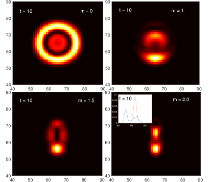
Figure 1: (Color online) Probability distribution $||\Psi(t_{j},x_{p},y_{q})||^{2}$ of the two-dimensional QW for a value $t=10$ of the timestep, and different values of $m$. The rest of parameters are fixed to $\lambda=60$, $h=70$, with the lattice parameter $\epsilon=0.04$. The inset in the last subfigure also shows the projected density profile along each direction of the lattice (red dot-dashed line represents the x-direction and blue dashed line the y-direction). The initial condition is a Gaussian wave packet $\Psi(0,x_{p},y_{q})=\sqrt{n(x_{p},y_{q})}\otimes(\frac{1}{\sqrt{2}},\frac{1}{\sqrt{2}})^{\top}$ centered at the point $(64,64)$, where the gaussian distribution $n(x_{p},y_{q})$ has a width $\delta=0.1$.

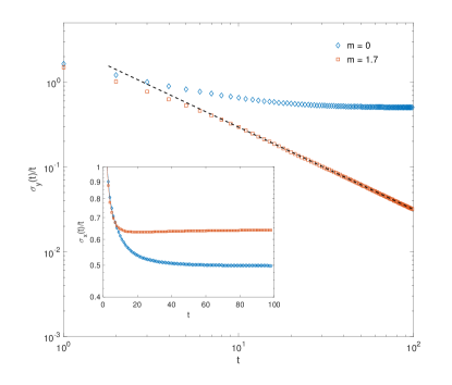
Figure 2: (Color online) Time evolution of the standard deviation divided by the timestep, i.e., $\sigma_{x}(t)/t$ (in the inset) and $\sigma_{y}(t)/t$, calculated independently along the $x$ and $y$ directions, for a localised (red squares) and a free fermion (blue diamonds). The initial condition is a Gaussian wave packet $\Psi(0,x_{p},y_{q})=\sqrt{n(x_{p},y_{q})}\otimes(0,1)^{\top}$ centered around $(128,128)$, and the parameters of the potential are $\lambda=60$ and $h=70$, with the lattice parameter $\epsilon=0.02$.

Equations (5) describe the evolution of a two-level system, e.g., a fermion in two dimensions, and it has been shown that each of them recover, in the continuous limit, the Dirac equation Di Molfetta et al. (2014), where the parameter $\theta_{q}$ corresponds to a position-dependent potential. Let us now consider $\bar{\theta}_{q}$ of the form:

$$\bar{\theta}_{q}=h\frac{m}{\sqrt{\lambda}}\tanh(\frac{mq}{\sqrt{2}}),$$ (9)

and notice that it corresponds to a narrow potential in the $q$-direction when $m$, the "effective mass" is sufficiently large.

Fig. 1 shows the evolved probability distribution of this 2D QW, starting from a symmetric Gaussian profile in both directions. As the mass is increased, the probability becomes strongly localized around the $y-$axis, while it evolves as a usual QW on the non-confining $x-$direction. This features are clearly seen in Fig. 2, where we have represented the standard deviation divided by the timestep, i.e., $\sigma_{x}(t)/t$ and $\sigma_{y}(t)/t$, calculated independently along the $x$ and $y$ directions. For $m=0$ (no confinement), both quotients tend to a constant, which corresponds to the normal spreading of a 2D QW in both directions. As $m$ increases, localization acts on the $y$- direction, and manifests as an exponential decay of $\sigma_{y}(t)/t$. On the other hand, the standard deviation corresponding to the $x$ axis behaves as a free-evolving QW, with a spreading velocity that depends on the parameters of the potential well.

As we show below, in the continuous limit equations (5) are in correspondence with Eq. (4), describing the propagation of a massless fermion in a space-time manifold $M^{(1+N,1)}$, the usual Minkowski space with $1+N$ spatial dimensions. When $m$ is non-vanishing, the fermion is confined inside a potential well, which is sufficiently narrow along $N$ directions and flat along the other one (in our case $N=1$).

Let us introduce new space-time coordinates $t_{j}$, $x_{p}$ and $y_{q}$ such that $t_{j}=j\epsilon$, $x_{p}=p\epsilon$ and $y_{q}=q\epsilon$. In the limit when $\varepsilon\longrightarrow 0$, these coordinates become continuous, labeled by $t$, $x$ and $y$, respectively. If we Taylor expand equations (5) around $\epsilon=0$, we recover the following equation:

$$\partial_{t}\Psi(t,x,y)=\left[\sigma_{z}\partial_{x}-\sigma_{y}\partial_{y}-i\sigma_{x}\bar{\theta}(y)\right]\Psi(t,x,y),$$ (10)

which can be recast in covariant form:

$$i\Gamma^{A}\partial_{A}\Psi+h\frac{m}{\sqrt{\lambda}}\tanh(\frac{my}{\sqrt{2}})\Psi=0,$$ (11)

where $\Gamma^{A}=\{\gamma^{\mu},\gamma^{c}\}$, $\mu=0,1$ and $\gamma^{c}=i\gamma^{5}=i\gamma^{0}\gamma^{1}=-i\sigma_{z}$. In this equation, $\gamma^{0}=-\sigma_{x}$, $\gamma^{1}=-i\sigma_{y}$. As can be easily seen, Eq. (11) takes the same form as (4) if we make the identification $x^{4}\longrightarrow y$ and $\varphi\longrightarrow\frac{m}{\sqrt{\lambda}}\tanh(\frac{my}{\sqrt{2}})$.

IV 3D Quantum Walks inside a 2+1 Domain Wall

The extension of the previous case to the higher dimensional case is straightforward. In this section we adopt the same techniques introduced in the last section but we double the spin Hilbert space, in order to recover the standard Dirac equation in 3+1 spacetime. Let us recall that in 3+1, gamma matrices appearing in equation (4), are four dimensional. In the Weyl representation they read:

$$\gamma^{0}=\begin{pmatrix}0&\mathbb{I}\\ \mathbb{I}&0\end{pmatrix}\ \ \gamma^{i}=\begin{pmatrix}0&\sigma^{i}\\ -\sigma^{i}&0\end{pmatrix}\ \gamma^{5}=\begin{pmatrix}-\mathbb{I}&0\\ 0&\mathbb{I}\end{pmatrix}.$$ (12)

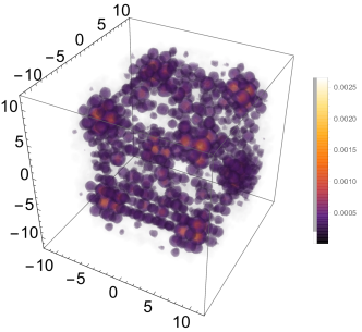
Figure 3: (Color online) Density plot in 3D at time $j=12$ with Gaussian initial wave packet $\Psi(0,x_{p},y_{q},z_{r})=\sqrt{n(x_{p},y_{q},z_{r})}\otimes(1,i,1,i)^{\top}$ centered around $(0,0)$, and for $m$ = $0$.

Now, consider the QW defined over discrete three-dimensional space, with axis $x$, $y$ and $z$. The discrete space points are labeled by $p$, $q$ and $r$, respectively, with $p,q,r\in\mathbb{Z}$. This QW is driven by an in-homogeneous coin acting on the spinor $\left(\psi^{1}_{j,p,q,r},\psi^{2}_{j,p,q,r}\right)^{\top}$, where each $\psi^{i}_{j,p,q,r}$ belongs to $\mathcal{H}_{\text{spin}}$ for $i=1,2$.

The evolution equations read:

$$\begin{bmatrix}\psi^{1}_{j+1,p,q,r}\\ \psi^{2}_{j+1,p,q,r}\end{bmatrix}\ =\Theta_{r}\mathcal{S}^{z}\mathcal{R}_{z}\mathcal{S}^{x}\mathcal{R}_{x}\mathcal{S}^{y}\mathcal{R}_{y}\begin{bmatrix}\psi^{1}_{j+1,p,q,r}\\ \psi^{2}_{j+1,p,q,r}\end{bmatrix},$$ (13)

where

$$\Theta_{r}=\begin{pmatrix}\cos\bar{\theta}_{r}\epsilon&i\sin\bar{\theta}_{r}\epsilon\\ i\sin\bar{\theta}_{r}\epsilon&\cos\bar{\theta}_{r}\epsilon\end{pmatrix}\otimes\mathbb{I}_{2},$$ (14)

and

$$\mathcal{S}^{i}=\begin{pmatrix}S^{i}&0\\ 0&{S^{i}}^{\dagger}\end{pmatrix} \hskip 42.67912pt\mathcal{R}_{i}=\begin{pmatrix}R_{i}&0\\ 0&R_{i}\end{pmatrix},$$ (15)

where the operators $S^{i}$ are the usual spin-dependent translations along each direction of the cubic lattice, and each unitary rotation $R_{i}$, for $i=x,y,z$ is an element of $U(2)$.

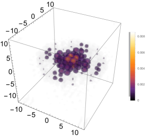
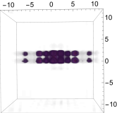
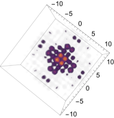
Figure 4: (Color online) Density plots in 3D at time $j=20$ with Gaussian initial wave packet $\Psi(0,x_{p},y_{q},z_{r})=\sqrt{n(x_{p},y_{q},z_{r})}\otimes(0,1,0,1)^{\top}$ centered around $(0,0)$. The parameters of the potential are $\lambda=90$, $h=4$ and $m$=$11$. The two subfigures at the bottom display the $x$-$z$ side view (left) and the $x$-$y$ side view (right) of the 3D density plot.

Notice that $\Theta_{r}$ encodes the coupling between the spinor components, and $\theta_{r}$ is an arbitrary position-dependent function, which can model either the mass term or any other scalar potential. If $\theta_{r}$ identically vanishes, Eq. (13) represents simply a couple of independent split-step QW operators acting on each component of the spinor. In the following, this mass-term is defined by Eq. (9), and will model the narrow potential in the $r$ direction, embedding a 3D QW in a 2D spacetime lattice.

In order to validate the model, we compute the formal continuous limit of Eq. (13) with same technique introduced in the previous section. Thus, let us introduce the new spatial coordinate $z_{r}$, such that $z_{r}=r\epsilon$, and again assume that in the limit when $\varepsilon\longrightarrow 0$, this coordinate, together with $t_{j}$, $x_{p}$, $y_{q}$, become continuous, labeled by $z$ and $t$, $x$, $y$, respectively. If we Taylor expand equations (13) around $\epsilon=0$, the zero order restricts the four-dimensional coins, $\mathcal{R}_{i}=R_{i}\otimes\mathbb{I}_{2}$:

$$\begin{bmatrix}\psi^{1}\\ \psi^{2}\end{bmatrix}\ =\mathcal{R}_{z}\mathcal{R}_{x}\mathcal{R}_{y}\begin{bmatrix}\psi^{1}\\ \psi^{2}\end{bmatrix}+O(\epsilon),$$ (16)

which leads to the condition

$$\mathcal{R}_{z}\mathcal{R}_{x}\mathcal{R}_{y}=\mathbb{I}_{4}.$$ (17)

Then the first order term of the Taylor expansion reads:

$$\partial_{t}\begin{bmatrix}\psi^{1}\\ \psi^{2}\end{bmatrix}\ =(B_{z}\partial_{z}+B_{x}\partial_{x}+B_{y}\partial_{y}+iB_{0}\bar{\theta}(z))\begin{bmatrix}\psi^{1}\\ \psi^{2}\end{bmatrix}+O(\epsilon),$$ (18)

where

$$B_{z}=Z\mathcal{R}_{z}\mathcal{R}_{x}\mathcal{R}_{y}$$

$$B_{x}=\mathcal{R}_{z}Z\mathcal{R}_{x}\mathcal{R}_{y}$$

$$B_{y}=\mathcal{R}_{z}\mathcal{R}_{x}Z\mathcal{R}_{y},$$ (19)

and

$$B_{0}=\sigma_{x}\otimes\mathbb{I}_{2}$$

$$Z=\mathbb{I}_{2}\otimes\sigma_{z}.$$ (20)

Now, comparing Eq. (18) with equation (4) we derive - up to a U(2) rotation - the explicit form of each rotation $\mathcal{R}_{i}$. In particular, we need to satisfy $\gamma^{0}\gamma^{1}=B_{x}$, $\gamma^{0}\gamma^{2}=B_{y}$ and $\gamma^{0}\gamma^{3}=B_{z}$, which leads to:

$$R_{x}=\frac{1}{\sqrt{2}}\begin{pmatrix}1&1\\ 1&-1\end{pmatrix}\hskip 42.67912ptR_{z}=\frac{1}{\sqrt{2}}\begin{pmatrix}1&-i\\ i&-1\end{pmatrix}\hskip 7.11317pt$$

$$R_{y}=R_{x}R_{z}.\hskip 85.35826pt$$ (21)

Thus, numerical simulations of the above QW can model the behavior of a fermion in a 3+1 space time. In particular, in Fig. 3, the quantum walker spreads on the 3D cubic lattice, starting from a symmetric initial condition, recovering in the continuous limit, a massless fermion in vacuum ($\bar{\theta}$ = $0$). In contrast, Fig. 4 shows the evolved probability distribution of this 3D QW when the mass-term is different from zero and position-dependent. As in the lower dimensional case, the probability dynamically localises on the $x$-$y$ plane, and corresponds to a standard 2D QW, while it possesses a finite size on the $z$-direction, which typically decreases with the lattice parameter $\epsilon$.

V Discussion

In this paper we have studied the properties of a two and a three dimensional QW that are inspired by the idea of a brane-world model put forward by Rubakov and Shaposhnikov Rubakov and Shaposhnikov (1983). In that model, particles are dynamically confined in the brane due to the interaction with a scalar field. We translated this model into an alternate QW with a coin that depends on the external field, with a dependence which mimics a domain wall solution. As in the original model, fermions (in our case, the walker), become confined in one of the dimensions, while they can move freely on the “ordinary” dimensions. In this way, we can think of the QW as a possibility to simulate brane models of quantum field theories. In the opposite direction of thought, we obtain a QW that shows localization, not from random noise on the lattice or from a periodic coin, as in previous models, but from a coin which changes in space in a regular, non periodic, manner. In our opinion, this interplay between QWs and high energy theories can be beneficial for both fields.

VI Acknowledgements

This work has been supported by the Spanish Ministerio de Educación e Innovación, MICIN-FEDER project FPA2014-54459-P, SEV-2014-0398 and Generalitat Valenciana grant GVPROMETEOII2014-087.

References

- Rubakov and Shaposhnikov (1983) V. Rubakov and M. Shaposhnikov, Physics Letters B 125, 136 (1983).
- Y. Aharonov, L. Davidovich (1993) N. Z. Y. Aharonov, L. Davidovich, Physical Review A 48, 1687 (1993), arXiv:1207.4535v1 .
- Farhi and Gutmann (1998) E. Farhi and S. Gutmann, Phys. Rev. A 58, 915 (1998).
- Grossing and Zeilinger (1988) G. Grossing and A. Zeilinger, Complex Systems 2, 197 (1988).
- Kempe (2003) J. Kempe, Contemporary Physics 44, 307 (2003), arXiv:0303081v1 [quant-ph] .
- Bloch et al. (2012) I. Bloch, J. Dalibard, and S. Nascimbene, Nature Physics 8, 267 (2012).
- Childs (2009) A. M. Childs, Phys. Rev. Lett. 102, 180501 (2009).
- Lovett et al. (2010) N. B. Lovett, S. Cooper, M. Everitt, M. Trevers, and V. Kendon, Phys. Rev. A 81, 042330 (2010).
- Ambainis (2003) A. Ambainis, International Journal of Quantum Information 1, 507 (2003).
- Magniez et al. (2011) F. Magniez, A. Nayak, J. Roland, and M. Santha, SIAM Journal on Computing 40, 142 (2011).
- Kitagawa et al. (2012) T. Kitagawa, M. A. Broome, A. Fedrizzi, M. S. Rudner, E. Berg, I. Kassal, A. Aspuru-Guzik, E. Demler, and A. G. White, Nature communications 3, 882 (2012).
- Arnault et al. (2016) P. Arnault, G. Di Molfetta, M. Brachet, and F. Debbasch, Phys. Rev. A 94, 012335 (2016).
- Genske et al. (2013) M. Genske, W. Alt, A. Steffen, A. H. Werner, R. F. Werner, D. Meschede, and A. Alberti, Physical review letters 110, 190601 (2013).
- Molfetta and Pérez (2016) G. D. Molfetta and A. Pérez, New Journal of Physics 18, 103038 (2016).
- Schreiber et al. (2012) A. Schreiber, A. Gábris, P. P. Rohde, K. Laiho, M. Štefaňák, V. Potoček, C. Hamilton, I. Jex, and C. Silberhorn, Science 336, 55 (2012).
- Côté et al. (2006) R. Côté, A. Russell, E. E. Eyler, and P. L. Gould, New Journal of Physics 8, 156 (2006).
- Anderson (1956) P. W. Anderson, Phys. Rev. 109 (1956).
- Aubry and André (1980) S. Aubry and G. André, Ann. Israel Phys. Soc 3, 18 (1980).
- Grempel et al. (1982) D. R. Grempel, S. Fishman, and R. E. Prange, Phys. Rev. Lett. 49, 833 (1982).
- Lahini et al. (2009) Y. Lahini, R. Pugatch, F. Pozzi, M. Sorel, R. Morandotti, N. Davidson, and Y. Silberberg, Phys. Rev. Lett. 103, 013901 (2009).
- Joye and Merkli (2010) A. Joye and M. Merkli, Journal of Statistical Physics 140, 1025 (2010).
- Schreiber et al. (2011) A. Schreiber, K. N. Cassemiro, V. Potoček, A. Gábris, I. Jex, and C. Silberhorn, Phys. Rev. Lett. 106, 180403 (2011).
- Crespi et al. (2013) A. Crespi, R. Osellame, R. Ramponi, V. Giovannetti, R. Fazio, L. Sansoni, F. De Nicola, F. Sciarrino, and P. Mataloni, Nature Photonics 7, 322 (2013), arXiv:arXiv:1304.1012v1 .
- Navarrete-Benlloch et al. (2007) C. Navarrete-Benlloch, A. Pérez, and E. Roldán, Physical Review A - Atomic, Molecular, and Optical Physics 75, 1 (2007), arXiv:0604084 [quant-ph] .
- Shikano and Katsura (2010) Y. Shikano and H. Katsura, Phys. Rev. E 82, 031122 (2010).
- Inui et al. (2004) N. Inui, Y. Konishi, and N. Konno, Phys. Rev. A 69, 052323 (2004).
- Kaluza (1921) T. Kaluza, Sitzungsber. Preuss. Akad. Wiss. Berlin (Math. Phys.) K1, 966 (1921).
- Klein (1926) O. Klein, Zeitschrift für Physik 37, 895 (1926).
- Arkani-Hamed et al. (1999) N. Arkani-Hamed, S. Dimopoulos, and G. Dvali, Phys.Rev. D 59, 086004 (1999), hep-ph/9807344 .
- Di Molfetta et al. (2014) G. Di Molfetta, M. Brachet, and F. Debbasch, Physica A: Statistical Mechanics and its Applications 397, 157 (2014).