Spin-orbital order in undoped manganite LaMnO₃ at finite temperature

Abstract

We investigate the evolution of spin and orbital order in undoped LaMnO₃ under increasing temperature with a model including both superexchange and Jahn-Teller interactions. We used several cluster mean field calculation schemes and find coexisting $A$-type antiferromagnetic ($A$-AF) and $C$-type alternating orbital order at low temperature. The value of the Jahn-Teller coupling between strongly correlated $e_{g}$ orbitals is estimated from the orbital transition temperature at $T_{\rm OO}\simeq 780$ K. By a careful analysis of on-site and on-bond correlations we demonstrate that spin-orbital entanglement is rather weak. We have verified that the magnetic transition temperature is influenced by entangled spin-orbital operators as well as by entangled orbital operators on the bonds but the errors introduced by decoupling such operators partly compensate each other. Altogether, these results justify why the commonly used disentangled spin-orbital model is so successful in describing the magnetic properties and the temperature dependence of the optical spectral weights for LaMnO₃.
Published in: Physical Review B 94, 214426 (2016).

I Introduction

Recent extensive work on transition metal oxides has demonstrated a strong interrelationship between spin order and orbital order, resulting in phase diagrams of great complexity for undoped compounds with active orbital degrees of freedom Tok00 . A good example is LaMnO₃, the parent compound of colossal magnetoresistance, where thorough experimental work has produced exceptionally detailed information on the phase diagrams of the $R$MnO₃ manganites (where $R$=Lu, Yb,$\dots$, La), yet the interplay between spin and orbital degrees of freedom is puzzling and could not be resolved by the theory so far Goode . This difficulty follows in general from the coupling to the lattice via the Jahn-Teller (JT) effect and partly from spin-orbital quantum fluctuations Fei97 ; Kha00 ; Kha01 ; Kha04 ; Kha05 which contribute to superexchange Kug82 ; Ole05 ; Hor08 ; Woh11 ; Brz15 and are amplified in the presence of spin-orbital entanglement on superexchange bonds Ole12 ; Rex12 ; You15 . The prominent example are the perovskite vanadium oxides where the temperature dependence of optical spectral weights Miy02 and the phase diagram Fuj10 could be understood in the theory only by an explicit treatment of entanglement Kha04 ; Hor08 . It is therefore of fundamental importance to consider simultaneously quantum spin and orbital degrees of freedom when investigating the possibility of spin-orbital order.

Although ordered spin-orbital states occur in many cases including LaMnO₃ Dag01 ; Tok06 , disordered quantum phases are very challenging, such as spin Bal10 ; Bal16 or orbital Kha00 ; Fei05 liquids when one of the two degrees of freedom is frozen. Another disordered state is a quantum spin-orbital liquid Nor08 ; Karlo ; Nas12 ; Sel14 ; Mil14 , where spin-orbital order is absent and occupied (by electrons or holes) spin-orbital states are randomly chosen by electrons. Previous attempts to find a spin-orbital liquid in the Kugel-Khomskii model Fei97 or in LiNiO₂ Ver04 turned out to be unsuccessful, and it was established that instead: (i) novel types of exotic spin-orbital order emerge from entanglement in the Kugel-Khomskii model Brz12 , and (ii) spin and orbital interactions are of quite different strengths in LiNiO₂ and the reasons behind the absence of magnetic long range order are more subtle Rei05 . Therefore, the right strategy is to investigate whether ordered states may occur and to what extent strong spin-orbital coupling (including possible entanglement) influences the spin and orbital phase transitions.

Here we focus on LaMnO₃, a Mott insulator with Mn³⁺ ions in $t_{2g}^{3}e_{g}^{1}$ configuration with high $S=2$ spin state stabilized by Hund’s exchange. The singly occupied $e_{g}$ orbitals are the orbital degrees of freedom which order below an orbital transition at $T_{\rm OO}\simeq 780$ K, recognized as a strong JT instability when cooperative distortions of oxygen octahedra occur and induce alternating orbital (AO) order Goo55 ; Fei98 ; Nan10 . Antiferromagnetic (AF) order of $A$-type ($A$-AF), i.e., AF phase with ferromagnetic (FM) $(a,b)$ planes staggered along the $c$ cubic axis, occurs below the Néel temperature $T_{N}\simeq 140$ K Kov10 . The purpose of this paper is to provide a comprehensive and unbiased scenario of these two phase transitions starting from the spin-orbital model of Ref. Fei99 using the realistic parameters.

Up to now, to the best of our knowledge, the phase transitions in LaMnO₃ were investigated only using classical on-site mean field (MF) theory which factorizes intersite spin and orbital correlations. Indeed, the $A$-AF phase with FM planes was obtained for LaMnO₃ Fei99 , and the orbital excitations were described within the orbital model and investigated at zero temperature vdB99 . Unfortunately, no thermal analysis of the spin-orbital model for LaMnO₃ was performed so far beyond the early MF study Fei99 , where the importance of orbital interactions induced by JT distortions was pointed out. This result is confirmed by calculations of the transition temperature from the superexchange mechanism by using the local density approximation combined with dynamical mean field method Pav10 . Below we provide evidence that going beyond the on-site MF theory is necessary to get a physically correct insight into the onset of $C$-type AO order below the orbital phase transition and its changes below the magnetic one. We analyze the nature of orbital states occupied by $e_{g}$ electrons in LaMnO₃.

The main purpose of this work is to carry out a systematic and consistent analysis of the effective spin-orbital model for LaMnO₃ within the cluster MF approach. In particular, of primary importance is to establish the orbital order by working out the value of orbital mixing angle (and its temperature dependence). The second objective of this work is to evaluate spin-orbital entanglement — both for (i) on-site and (ii) on-bond correlations. As we show below the obtained results justify a posteriori the commonly used spin-orbital decoupling approximation. The third objective is to establish the range for the JT coupling constant. The complexity of the model gives rise to technical benchmark. The technical objective is to verify to what extent the cluster calculations are reliable.

The paper is organized as follows: In Sec. II we introduce the spin-orbital model for LaMnO₃ and present a detailed discussion of various terms contributing to superexchange in Sec. II.2. The JT terms and parameters are presented in Sec. II.3. Next we introduce the essential features of a MF analysis of spin and orbital order in Sec. III and discuss the main problems related to the analysis of coexisting $A$-AF and $C$-AO order in Sec. III.2. Cluster MF approaches are presented in Sec. IV. In Sec. V we present the numerical results obtained using different clusters with disentangled interactions and also entangled spin-orbital bond for magnetic and orbital transition, see Sec. V.2. Next we give spin and orbital bond correlations and exchange constants, see Secs. V.3-V.4, as well as optical spectral weights, see Sec. V.5. In Sec. VI we investigate on-site (Sec. VI.1) and on-bond (Sec. VI.2) spins-orbital entanglement and finally its impact on the value of Néel transition temperature, see Sec. VI.3. This analysis allows us to formulate general conclusions concerning the role of entanglement in the properties of LaMnO₃. The summary and conclusions are given in Sec. VII.

II Model

The model analyzed in this work consists of two terms: (i) the superexchange interaction $H_{J}$ derived from $d_{i}^{4}d_{j}^{4}\rightleftharpoons d_{i}^{5}d_{j}^{3}$ charge excitations on bonds between nearest neighbor Mn³⁺ ions and (ii) the JT term $H_{\rm JT}$ which follows from local lattice distortions triggered by the JT coupling. The Hamiltonian reads,

$${\cal H}=H_{J}+\mathbf{1}_{\mbox{spin}}\otimes H_{\rm JT}.$$ (1)

The superexchange part $H_{J}$ was derived by considering charge excitations for both $e_{g}$ and $t_{2g}$ electrons Fei99 , where it was shown that it predicts $A$-AF order for the realistic parameters. Although the charge excitations on oxygen orbitals play a role Ole05 , its generic form which includes such excitations only in an effective way was successfully used to interpret the temperature evolution of spectral weights measured in the optical spectroscopy Kov10 . The model Eq. (1) poses a difficult many-body problem. We treat it here in several approximations discussed below and investigate to what extent spins and orbitals may be separated from each other.

II.1 Orbital projections

To establish formulas for $H_{J}$ and $H_{\rm JT}$ one has to introduce first orbital projection operators for $e_{g}$ orbital degree of freedom. They are the same as for the Kugel-Khomskii model for KCuF₃ Ole00 . We start with on-site orbital projection operators at site $i$:

$$P_{i}^{\zeta_{\gamma}}\equiv|i\zeta_{\gamma}\rangle\langle i\zeta_{\gamma}|,\qquad P_{i}^{\xi_{\gamma}}\equiv|i\xi_{\gamma}\rangle\langle i\xi_{\gamma}|.$$ (2)

Here the orbitals $\{|\zeta_{\gamma}\rangle,|\xi_{\gamma}\rangle\}$ form an orthogonal basis at site $i$ consisting of a directional orbital $|\zeta_{\gamma}\rangle$ and a planar orbital $|\xi_{\gamma}\rangle$. They depend on the cubic axis index $\gamma$:

$|\zeta_{a}\rangle=|3x^{2}-r^{2}\rangle$,	$|\xi_{a}\rangle=|y^{2}-z^{2}\rangle$,
$|\zeta_{b}\rangle=|3y^{2}-r^{2}\rangle$,	$|\xi_{b}\rangle=|z^{2}-x^{2}\rangle$,
$|\zeta_{c}\rangle=|3z^{2}-r^{2}\rangle$,	$|\xi_{c}\rangle=|x^{2}-y^{2}\rangle$.

The projection operators exhaust the orbital space, i.e.,

$$P_{i}^{\zeta_{\gamma}}+P_{i}^{\xi_{\gamma}}=1.$$ (3)

Depending on the bond direction on which the superexchange $J_{J}$ or JT interaction $H_{\rm JT}$ acts, one has to choose $\gamma=a,b,c$. Then, it is necessary to introduce projection operators for a bond along the cubic axis $\gamma$:

$$\mathcal{P}^{\zeta\xi}_{\langle ij\rangle\parallel\gamma} \equiv 2P_{(i}^{\zeta_{\gamma}}P_{j)}^{\xi_{\gamma}}\equiv P_{i}^{\zeta_{\gamma}}P_{j}^{\xi_{\gamma}}+P_{i}^{\xi_{\gamma}}P_{j}^{\zeta_{\gamma}},$$ (4)

$$\mathcal{P}^{\zeta\zeta}_{\langle ij\rangle\parallel\gamma} \equiv 2P_{i}^{\zeta_{\gamma}}P_{j}^{\zeta_{\gamma}},$$ (5)

$$\mathcal{P}^{\xi\xi}_{\langle ij\rangle\parallel\gamma} \equiv 2P_{i}^{\xi_{\gamma}}P_{j}^{\xi_{\gamma}}.$$ (6)

Note that the operator $2P_{(i}^{\zeta_{\gamma}}P_{j)}^{\xi_{\gamma}}$ refers to a symmetrized product of two projection operators on sites $i$ and $j$. Such operators characterize the processes which contribute to various interaction terms, see below. The factor of 2 in Eqs. (5) and (6) is introduced for a more compact notation below as the charge excitations used to derive the superexchange involve intersite excitations by hopping which couples two directional $\{|i\zeta_{\gamma}\rangle,|j\zeta_{\gamma}\rangle\}$ orbitals at sites $i$ and $j$ only Ole00 . Actually, the bond operators Eqs. (4)-(6) are not independent and obey the constraint which may serve to determine one of them from the other two,

$$\mathcal{P}^{\zeta\zeta}_{\langle ij\rangle}+2\mathcal{P}^{\zeta\xi}_{\langle ij\rangle}+\mathcal{P}^{\xi\xi}_{\langle ij\rangle}=2.$$ (7)

II.2 Spin-orbital superexchange

The superexchange part $H_{J}$ of the effective Hamiltonian ${\cal H}$ (1) arises from various virtual excitations to Mn²⁺ states with $d^{5}$ electronic configuration Fei99 . The charge excitations $d_{i}^{4}d_{j}^{4}\rightleftharpoons d_{i}^{5}d_{j}^{3}$ obtained from $e_{g}$ electron hopping may generate a high-spin (HS) ${}^{6}A_{1}$ state or low-spin (LS) ${}^{4}A_{1}$, ${}^{4}E$ and ${}^{4}A_{2}$ states. The remaining Mn⁴⁺ ion is always in HS ${}^{4}A_{1}$ state. In addition, there are also charge excitations by a transfer of a $t_{2g}$ electron between sites $i$ and $j$. The $t_{2g}$ levels are half filled in the Mn³⁺ $d^{4}$ ground state, so only LS excited states are generated by the $t_{2g}$ electron hopping as the orbital flavor is again conserved. We list here the excited $d_{i}^{5}d_{j}^{3}$ states pairwise for $d_{i}^{5}d_{j}^{3}$: $(^{4}T_{1},^{4}T_{1})$, $(^{4}T_{1},^{4}T_{2})$, $(^{4}T_{2},^{4}T_{1})$, and $(^{4}T_{2},^{4}T_{2})$.

The leading part of the superexchange Hamiltonian $H_{J}$ describes the interactions obtained from charge excitations by $e_{g}$ electrons and is parameterized by four physical parameters: (i) hopping element for $e_{g}$ electrons $t$ between two $|\zeta\rangle$ orbitals oriented along the considered bond $\langle ij\rangle$, (ii) on-site Coulomb repulsion energy $U$, (iii) Hund’s exchange $J_{H}^{e}$ for $e_{g}$ electrons, and (iv) Hund’s exchange $J_{H}^{t}$ for $t_{2g}$ electrons. In fact, $U$ and $J_{H}^{e}$ may be expressed by three Racah parameters Ole05 : $U=A+4B+3C$, $J_{H}^{e}=4B+C$. For charge excitations generated by $t_{2g}$ electrons Hund’s exchange is somewhat smaller, $J_{H}^{t}=3B+C$, and the hopping for a $\pi$ bond is reduced to $\beta t$, where $\beta=1/9$. All the excitation energies are collected in Table 1.

Table 1: The $d_{i}^{5}$ excited states and their excitation energies $E_{n}$ found from the analysis of $d_{i}^{4}d_{j}^{4}\leftrightarrows d_{i}^{5}d_{j}^{3}$ charge excitations in undoped LaMnO₃. Parameters to calculate $E_{n}$ as in Eqs. (16) and (17). The experimental energies $E_{\textrm{exp}}$ are from Ref. Kov10 .

		excitation energy $E_{n}$
orbital	term	$E_{n}$ (theory)	$E_{n}$ (eV)	$E_{\textrm{exp}}$ (eV)
$e_{g}$	${}^{6}A_{1}$	$U-3J_{H}^{e}$	1.93	$2.0\pm 0.1$
	${}^{4}A_{1}$	$U+3J_{H}^{e}/4$	4.52	$4.3\pm 0.2$
	${}^{4}E$	$U+5J_{H}^{e}/4$	4.86	$4.6\pm 0.2$
	${}^{4}A_{2}$	$U+13J_{H}^{e}/4$	6.24	$6.1\pm 0.2$
$t_{2g}$	$(^{4}T_{1},^{4}T_{2})$	$U+5J_{H}^{t}/4$	4.74	$3.9\pm 0.1$
	$(^{4}T_{2},^{4}T_{2})$	$U+9J_{H}^{t}/4$	5.33	$4.4\pm 0.1$
	$(^{4}T_{1},^{4}T_{1})$	$U+11J_{H}^{t}/4$	5.62	$4.8\pm 0.1$
	$(^{4}T_{2},^{4}T_{1})$	$U+15J_{H}^{t}/4$	6.21	$5.7\pm 0.5$

Whereas there are four physical parameters that control the Hamiltonian $H_{J}$, the model has three independent parameters. The superexchange constant is Fei99 ,

$$J=\frac{4t^{2}}{U},$$ (8)

where $t$ is the hopping element for a bond $\langle ij\langle$ (via oxygen ions) between two directional $e_{g}$ orbitals $\{|\zeta_{i\gamma}\rangle,|\zeta_{j\gamma}\rangle\}$, e.g. $|3z^{2}-r^{2}\rangle$ orbitals along the $c$ axis. To specify various contributions we introduce

$$\eta_{e}=\frac{J_{H}^{e}}{U},\hskip 19.91684pt\eta_{t}=\frac{J_{H}^{t}}{U}.$$ (9)

to distinguish between Hund’s exchange for $e_{g}$ and $t_{2g}$ electrons. This generates small changes of the superexchange Anderson contributions to $H_{J}$ considered before in Refs. Ole05 and Kov10 . The Goodenough contributions which stem from charge excitations on oxygen orbitals along Mn-O-Mn bonds Ole05 are neglected here in the effective model $H_{J}$.

Now, it it straightforward to write the formula for $H_{J}$ which includes the terms due to $e_{g}$ ($H_{e}$) and $t_{2g}$ ($H_{t}$) electron excitations,

$$H_{J}=H_{e}+H_{t},$$ (10)

where

$$\begin{split}H_{e}=J\sum_{\langle ij\rangle\parallel\gamma}&\Bigg{\{}-\frac{1}{40}r_{1}\big{(}\vec{S}_{i}\cdot\vec{S}_{j}+6\big{)}\mathcal{P}^{\zeta\xi}_{\langle ij\rangle}\\ &+\left[\frac{1}{64}r_{3}+\frac{3}{320}r_{2}\right]\big{(}\vec{S}_{i}\cdot\vec{S}_{j}-4\big{)}\mathcal{P}^{\zeta\xi}_{\langle ij\rangle}\\ &+\left[\frac{1}{64}r_{4}+\frac{1}{64}r_{5}\right]\big{(}\vec{S}_{i}\cdot\vec{S}_{j}-4\big{)}\mathcal{P}^{\zeta\zeta}_{\langle ij\rangle}\Bigg{\}},\end{split}$$ (11)

and

$$H_{t}=J\beta\sum_{\langle ij\rangle}\frac{1}{8}r_{t}\big{(}\vec{S}_{i}\cdot\vec{S}_{j}-4\big{)}.$$ (12)

The multiplet structure of $e_{g}$ excited states, see Table 1, is given by

$$r_{1} = \frac{1}{1-3\eta_{e}},\hskip 42.67912ptr_{2}=\frac{1}{1+3\eta_{e}/4},$$

$$r_{3} = r_{4}=\frac{1}{1+5\eta_{e}/4},\qquad r_{5}=\frac{1}{1+13\eta_{e}/4}.$$ (13)

For excitations by a $t_{2g}$ electron we have to collect all the terms by projecting the excited configurations onto the eigenstates listed in Table 1. This results in a single coefficient,

$$r_{t}\!=\!\frac{1}{4}\left[\frac{1}{1+5\eta_{t}/4}\!+\!\frac{1}{1+9\eta_{t}/4}\!+\!\frac{1}{1+11\eta_{t}/4}\!+\!\frac{1}{1+15\eta_{t}/4}\right].$$ (14)

II.3 Jahn-Teller terms and parameters

The JT Hamiltonian $H_{\rm JT}$ describes the coupling between the adjacent sites via the mutual octahedron distortion. We invoke here the simple quantum 120° model to control it. We note that JT effect is connected with the oxygen atoms displacements which result in longer and shorter Mn-O bonds but leave the manganese positions undisturbed.

The correct form of the effective interactions between the occupied $e_{g}$ orbitals depends only on the symmetries of the Mn-O octahedra. A classical derivation of the effective orbital-orbital interactions between the neighboring manganese ions was presented by Halperin and Englman Hal71 . After transforming these interactions to the bond orbital projection operators Eqs. (4)-(6), the formula that describes $H_{\rm JT}$ reads as follows Fei99 :

$$H_{\rm JT}=\kappa\sum_{\langle ij\rangle}\left(\mathcal{P}^{\zeta\zeta}_{\langle ij\rangle}-2\mathcal{P}^{\zeta\xi}_{\langle ij\rangle}+\mathcal{P}^{\xi\xi}_{\langle ij\rangle}\right).$$ (15)

We remark that a full derivation of the orbital-orbital interaction (15) generated by the JT coupling is complicated Geh75 and here we limit ourselves to presenting the consequences of its simplified form (15) that follows from the classical derivation Hal71 . As a result, the JT term is controlled by a single parameter $\kappa$ that describes the rigidity of the oxygen positions (or magnitude of displacement caused by the adjacent Mn orbital state). If the oxygens were rigid and their positions were not influenced by manganese orbital states then $\kappa=0$, but in reality $\kappa>0$.

The choice of parameters which determine the superexchange has been extensively discussed in the past, for instance in Ref. Kov10 . Here we use the following values (all in eV):

$$t=0.37,\quad U=4.0,\quad J_{H}^{e}=0.69,\quad J_{H}^{t}=0.59,$$ (16)

to obtain the excitation energies given in Table 1. These values stay in reasonable agreement with the experimental values that are also listed in Table 1. In addition, we adopt here

$$\kappa=6\ {\rm meV}.$$ (17)

This value was chosen a posteriori to fit the value of the orbital transition temperature $T_{\rm OO}$. It confirms the earlier observation Oka02 that the JT coupling is just a fraction of $J=t^{2}/U\simeq 34$ meV, i.e., it is much smaller than the values suggested for $\kappa$ within the MF approach at the early stage of the theory, such as: $11$ meV Fei99 and $9.1$ meV Sik03 .

III Mean field treatment and beyond

III.1 Orbital state description

The simplest approach to the many-body problem posed by Eq. (1) is the MF approach where only single-site averages are introduced to investigate possible order. In spin space we consider the symmetry breaking along the $z$ axis, with $\langle S_{i}^{z}\rangle$ being the order parameter at site $i$. In a uniform phase the parameter $\langle S^{z}\rangle\equiv\langle S_{i}^{z}\rangle$ is a magnetic (spin) order parameter.

The orbital (pseudospin) state is completely described by density matrix

$$\rho\equiv\operatorname{Tr}^{\prime}\Big{(}|\Psi\rangle\langle\Psi|\Big{)}\in\mathbb{C}^{2\times 2}$$ (18)

where $\Psi$ denotes the complete wave function and $\operatorname{Tr}^{\prime}$ means that all but considered pseudospin degrees of freedom were integrated out. When the orbital basis,

$$|3z^{2}-r^{2}\rangle/\sqrt{6}\, \Rightarrow \begin{pmatrix}1\\ 0\end{pmatrix},$$ (19)

$$|x^{2}-y^{2}\rangle/\sqrt{2}\, \Rightarrow \begin{pmatrix}0\\ 1\end{pmatrix},$$ (20)

is chosen, the density operator $\rho$ is isomorphic to $2\times 2$ not negative-definite hermitian matrix with trace equal to one. For the sake of description of orbital (pseudospin) Bloch vector was invoked, i.e., vector $\vec{r}\in\mathbb{R}^{2}$ contained in closed unit disk for which

$$\rho=\frac{1}{2}\mathbf{1}_{2}+\frac{1}{2}\vec{r}\cdot\vec{\sigma},\qquad\text{where: }\vec{\sigma}=\begin{pmatrix}\sigma_{x}\\ \sigma_{z}\end{pmatrix}.$$ (21)

Then, the radius $r$ and the angle $\theta$ are introduced to replace the polar coordinates,

$$\vec{r}=r\begin{pmatrix}+\sin\theta\\ -\cos\theta\end{pmatrix},\quad\begin{array}[]{c}r\in[0,1],\\ \theta\in(-180\text{\textdegree},180\text{\textdegree}].\end{array}$$ (22)

In terms of $r$ and $\theta$ parameters one finds:

$$\langle\sigma_{x}\rangle =\text{Tr}(\sigma_{x}\rho)=+r\sin\theta,$$ (23)

$$\langle\sigma_{z}\rangle =\text{Tr}(\sigma_{z}\rho)=-r\cos\theta.$$ (24)

Note, that the pure states lie on the unit circle ($r=1$), and the corresponding wave vectors are equal to vdB99 ,

$$|\theta\rangle=\cos(\theta/2)|3z^{2}-r^{2}\rangle/\sqrt{6}+\sin(\theta/2)|x^{2}-y^{2}\rangle/\sqrt{2}.$$ (25)

The amplitude $r$ is considered as orbital order parameter.

III.2 Preliminary analysis of $A$-AF/$C$-AO order

At low temperature $A$-AF and $C$-AO order coexist in LaMnO₃. Let us start the analysis of the symmetry broken state with the FM $(a,b)$ planes (perpendicular to the cubic $c$ axis). In this case $\langle\vec{S}_{i}\cdot\vec{S}_{j}\rangle=+4$ for the classical bonds in the plane, and the only nonvanishing contribution from the superexchange Hamiltonian is the interaction involving the HS states. We observe that this part of Hamiltonian (11) is proportional to $\mathcal{P}^{\zeta\xi}_{\langle ij\rangle}$, and its coefficient is approximately equal to $-70$ meV. The JT effect enhances this interaction further. The interaction parallel to the $a$ axis prefers the pair of orbitals proportional to $|x^{2}\rangle$ and $|z^{2}-y^{2}\rangle$, respectively (with the mixing angle $\theta$ equal to $-120$° and $+60$°). At the same time the interaction parallel to the $b$ axis prefers the pair of orbitals proportional to $|y^{2}\rangle$ and $|z^{2}-x^{2}\rangle$ respectively (with the mixing angle $\theta$ equal to $+120$° and $-60$°). These interactions are frustrated. As a result of them the ground state emerges which involves AO order for the orbitals with mixing angle $\theta$ alternating between 90° and $-90$°.

In the AF direction for the bonds along the $c$ axis the problem is more subtle. In this case $\langle\vec{S}_{i}\cdot\vec{S}_{j}\rangle=-4$ in MF (i.e., neglecting quantum fluctuations) and superexchange terms for both HS and LS excitations are important. They are found in $H_{J}$ both as proportional to $\mathcal{P}^{\zeta\xi}_{\langle ij\rangle}$, and proportional to $\mathcal{P}^{\zeta\zeta}_{\langle ij\rangle}$. The former term proportional to $\mathcal{P}^{\zeta\xi}$ contributes with coefficient $\approx-35$ meV, while the JT effect enhances this interaction. This term favors AO order with $3z^{2}-r^{2}$ ($\theta=0$) and $x^{2}-y^{2}$ ($\theta=180$°) orbital pairs. But it is not strong enough and the pattern with $\theta$ equal to $\pm 90$° sustain. (In fact, this configuration is energetically not very bad for this interaction). In addition the term proportional to $\mathcal{P}^{\zeta\zeta}_{\langle ij\rangle}$ is present with negative coefficient. This interaction enhances the $|3z^{2}-r^{2}\rangle$ ($\theta=0$) contributions to the orbitals in the ground state. Due to these interactions the mixing angle $\theta$ is significantly lower than 90°.

We may check our tentative results against the crystallographic data Huang97 . We invoke here the results for polymorphic structure with symmetry $Pmna$ and lattice parameters: $a=5.7$Å, $b=7.7$Å, and $c=5.5$Å. The AO pattern in the FM planes should result in the alternating pattern of the octahedron distortions. Indeed, in real crystal such a distortion pattern was observed. The in-plane Mn-O bonds length are equal to $s=1.91$Å, $l=2.18$Å. What is more the Mn-O bonds perpendicular to the FM planes are longer than 1.91Å (their length is equal to $m=1.96$Å). It means that the alternating mixing angle $\theta$ is lower than 120°.

One may express the distortion in terms of $Q_{2}$ and $Q_{3}$ modes. The corresponding coefficients are equal to

$$Q_{2}=\frac{l-s}{\sqrt{2}},\qquad Q_{3}=\frac{2m-l-s}{\sqrt{6}}.$$ (26)

From $(Q_{2},Q_{3})$ one may evaluate the orbital mixing angle with the aid of identification

$$\big{(}Q_{2},Q_{3}\big{)}=|Q|\big{(}\sin\theta,\cos\theta\big{)}.$$ (27)

This leads to $\theta=108$°. We see that in real crystal $\theta$ is bigger than 90°; in contrast for our model where $\theta\leq 90$°.

We may guess two possible reasons for this discrepancy.

• We should note that in a crystal of LaMnO₃ not only JT effect is important. The JT effect is responsible for octahedron deformation but leaves the Mn positions undisturbed. When the adjacent Mn-Mn distances are not equal to each other the crystal-field interactions occur. In case of the analyzed crystal the adjacent Mn-Mn distances are equal for the Mn pairs belonging to one FM plane, but this distance is larger than the distance between adjacent Mn from two different FM planes. This means that there is one more interaction that plays a role. In this case this interaction prefers instead $|x^{2}-y^{2}\rangle$ orbitals ($\theta=180$°) and may result in boosting the value of the mixing angle. We do not consider this interaction within the present work.

• Due to anharmonicity of the JT interactions the potential achieves its minimum in $\theta=0$°, $\pm 120$°. This may result in boosting the mixing angle value (up to $120$°).

IV Cluster mean field approaches

IV.1 Beyond single-site mean field theory

In this work the model described by Eq. (1) is analyzed to figure out the orbital and spin temperature dependence, as well as the phase transition temperatures, $T_{\rm N}$ and $T_{\rm OO}$. We employ the cluster MF approach to investigate the interplay between these phase transitions in a more realistic way than in a single-site MF theory. As in previous modern applications of the cluster MF method Brz12 ; Alb11 ; Got16 , the considered cluster is embedded by the MF terms of its surrounding, and self-consistent conditions are imposed (to ensure that all the on-site mean values of surrounding vertices take their proper values). In presented calculations $A$-AF and $C$-AO order is assumed. It may be taken for granted as indeed this type of order gives the lowest energy in the ground state at $T=0$.

The smallest cluster that captures the point symmetry of considered Hamiltonian Eq. (1) (a chiral octahedral symmetry $\text{O}_{\text{h}}$) consists of 7 sites. Due to the big number of spin-orbital degrees of freedom per site ($5\times 2=10$) the corresponding space of states of the cluster is enormous ($10^{7}$). This makes it impossible to carry out exact (cluster) calculations. Thus, further approximations cannot be avoided. In this work two alternative further approximation (or calculation) schemes are invoked: (i) multi-single-bond scheme and (ii) spin-orbital decoupling scheme.

IV.2 Multi-single-bond calculation scheme

First calculation scheme, called here multi-single-bond scheme, is rooted in a single-bond calculation. As a first step a single calculation for one bond is performed to find the state of this bond immersed in its fixed environment. As the cubic directions are nonequivalent in symmetry-broken states, in elementary iteration of multi-single-bond scheme 6 single-bond calculations are carried out as there are 6 inequivalent (but symmetry related) bond types in the considered system. At the end of each elementary iteration all important single-site operator mean values are established as averages of mean values achieved from corresponding single-bond calculations (involving considered site). Iterations are repeated until convergence.

The main advantage of the multi-single-bond scheme is that it treats all the degrees of freedom on equal footing, including the spin-spin, orbital-orbital and spin-orbital interactions. The main disadvantage stems from the small cluster size — all the phase transition temperatures predicted by it are considerably overestimated.

Although multi-single-bond calculation scheme suffers from many problems it can provide some useful information. Firstly, with the aid of it we can evaluate mean values: $\langle S_{i}^{z}\sigma_{i}^{z}\rangle$, $\langle S_{i}^{z}S_{j}^{z}\sigma_{i}^{z}\sigma_{j}^{z}\rangle$, etcetera. Second, what is even more important, it can provide heuristic value of the error that occurs in calculations in which the spin and the orbital degrees of freedom are treated separately. To get appropriate error values one should compare result from this model with the result of the factorized model, i.e., modified in such away that all spin-orbital interactions are artificially broken into sums of two product operators and are disentangled.

IV.3 Decoupling calculation scheme

Second calculation scheme, called here decoupling scheme is rooted in a decoupling of the spin and the orbital degree of freedom. In this approach spin and orbital degrees of freedom are disentangled. In the elementary iteration step of the decoupling scheme one pure spin calculation and one pure orbital calculation are carried out. The pure orbital calculations Hamiltonian arises from Hamiltonian Eq. (1) after replacement of all the products of spin operators by the averages $\langle\vec{S}_{i}\cdot\vec{S}_{j}\rangle$ being scalar parameters (one parameter for one bond direction). Similarly, the pure spin calculations Hamiltonian arises from Hamiltonian Eq. (1) after replacement of all orbital projection operators $\mathcal{P}^{\zeta\xi}_{\langle ij\rangle\parallel\gamma}$ and $\mathcal{P}^{\zeta\zeta}_{\langle ij\rangle\parallel\gamma}$ by the scalar parameters. After such a replacement one ends up with the anisotropic spin model with exchange parameters $J_{ab}$ and $J_{c}$ for $S=2$ spins,

$$H_{S}=J_{ab}\sum_{\langle ij\rangle\parallel ab}\vec{S}_{j}\cdot\vec{S}_{j}+J_{c}\sum_{\langle ij\rangle\parallel c}\vec{S}_{j}\cdot\vec{S}_{j}.$$ (28)

Here we use a short-hand notation and label by $J_{ab}$ exchange interactions in $(a,b)$ planes, $J_{a}=J_{b}$, as the bonds along the $a$ and $b$ cubic axes are equivalent. In this case the $J_{\gamma}$’s constants are given by

$$J_{\gamma}=J\Bigg{\{}\left[-\frac{1}{40}r_{1}+\frac{1}{64}r_{3}+\frac{3}{320}r_{2}\right]\left\langle\mathcal{P}^{\zeta\xi}_{\langle ij\rangle}\right\rangle\\ +\left[\frac{1}{64}r_{4}+\frac{1}{64}r_{5}\right]\left\langle\mathcal{P}^{\zeta\zeta}_{\langle ij\rangle}\right\rangle+\beta\frac{1}{8}r_{t}\Bigg{\}},$$ (29)

for $i$ and $j$ forming a bond $\langle ij\rangle\parallel\gamma$.

The pure spin Hamiltonian has some parameters which are connected with the orbital state, and the pure orbital Hamiltonian has some parameters which are connected with the spin state. At the end of each elementary iteration of the present decoupling scheme, the collection of new parameters is established. The procedure is carried out until its full convergence.

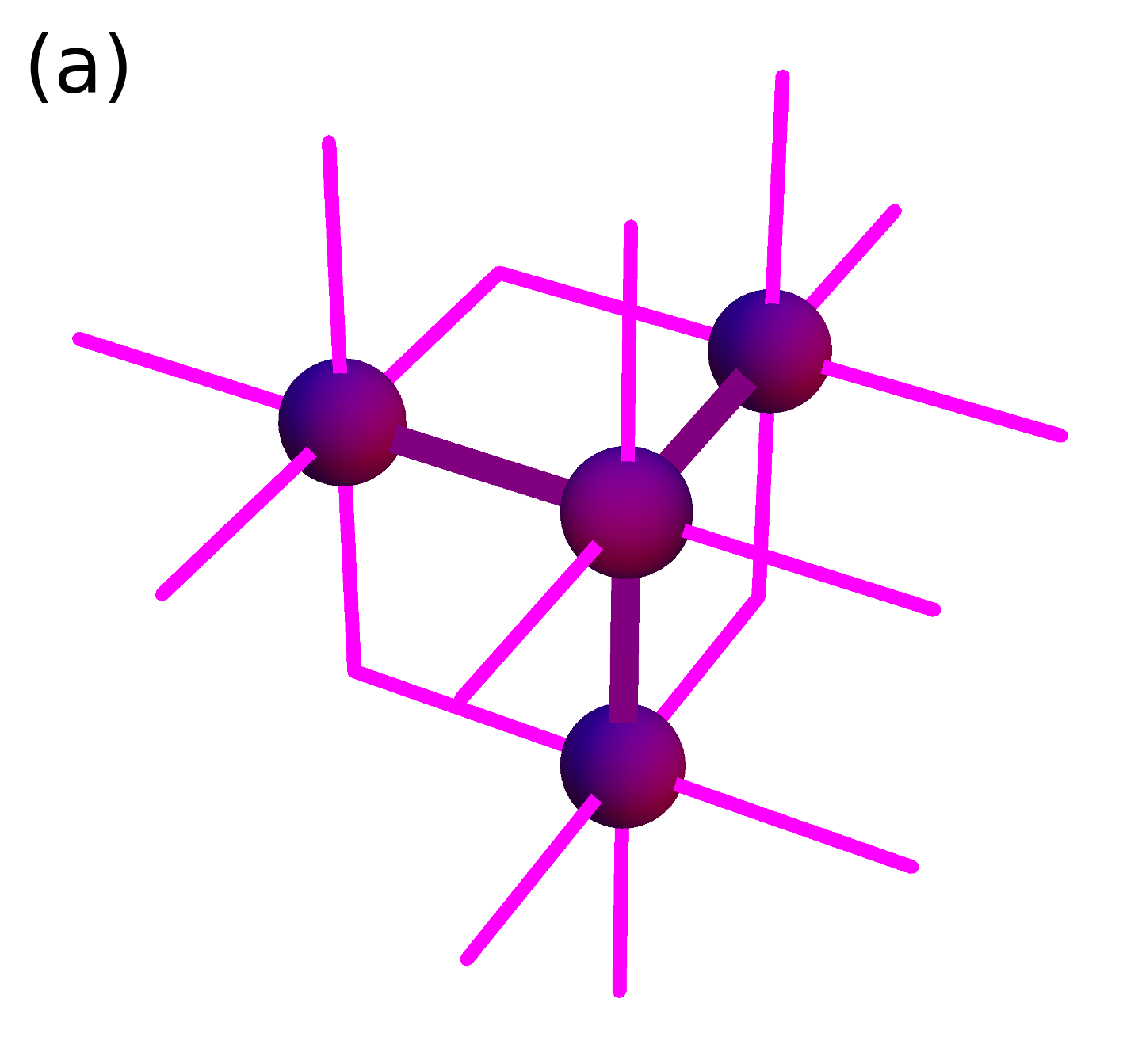
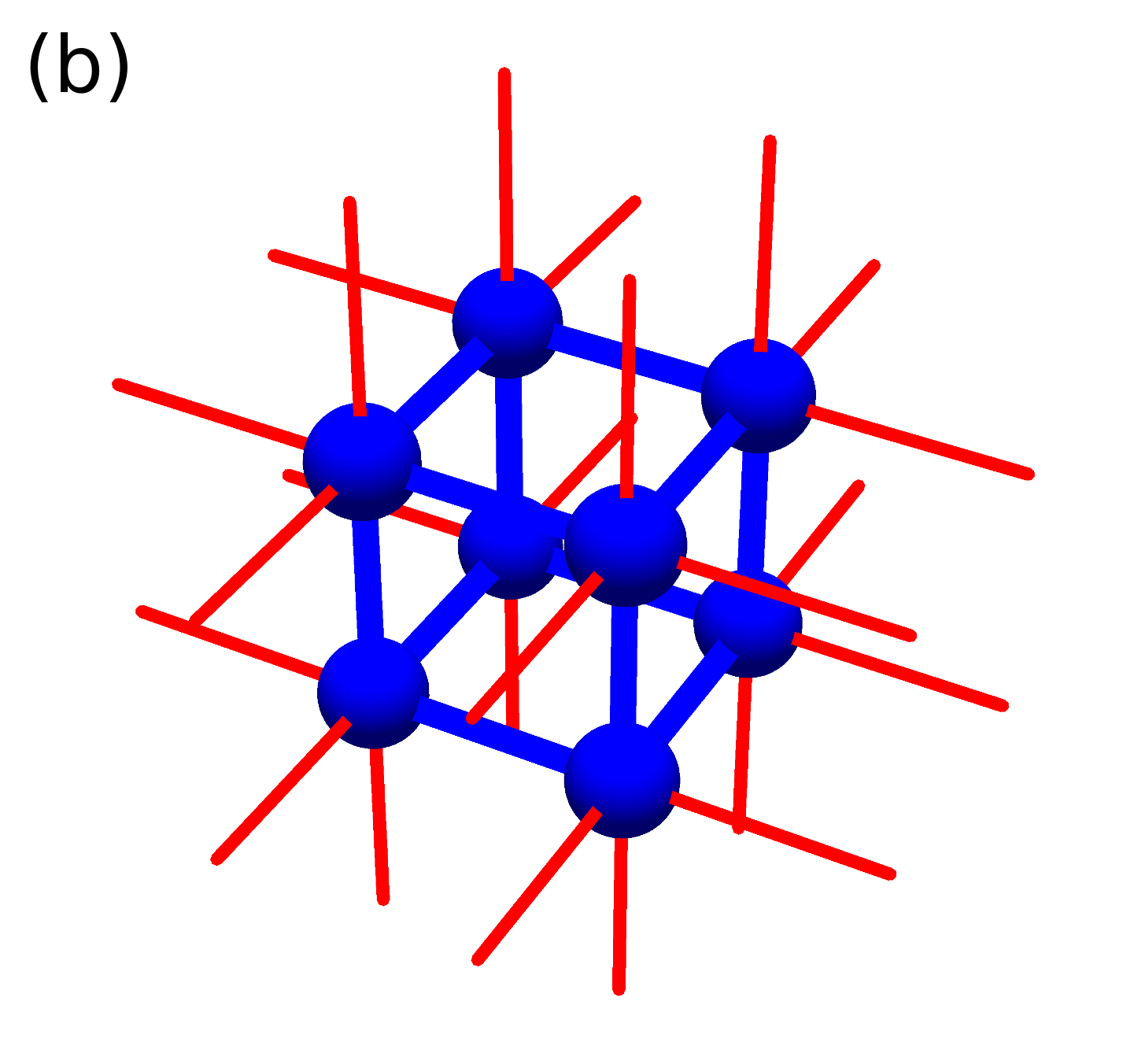
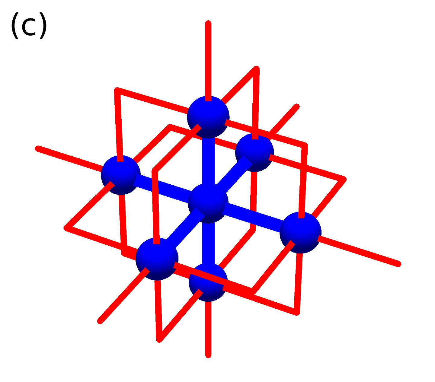
Figure 1: The clusters used in the calculations: (a) sputnik cluster for pure spin calculation, and clusters for pure orbital calculations, (b) cubic and (c) hedgehog. The vertices belonging to the cluster are depicted as spheres. The thick segments that link the spheres represent the two-sites interactions; the remaining lines represent interactions that are considered in MF approximation.

At the first glance is seems that method rooted in solely pure orbital calculation would be valid for temperatures well above $T_{\rm N}$. In fact, well above the onset of spin order at $T_{\rm N}$ the average spin order parameter $\langle S^{z}\rangle$ is equal to zero and the spin fluctuations on bonds seem to have marginal impact. Namely, there is a temptation to build orbital model by changing the spin operators into some given values and leave the orbital operators unchanged. This simple concept is however misleading due to quite a complicated reason. If one replaces both $\langle\vec{S}_{i}\cdot\vec{S}_{j}\rangle_{ab}$ and $\langle\vec{S}_{i}\cdot\vec{S}_{j}\rangle_{c}$ by the same value (e.g. zero) one creates the Hamiltonian that possesses additional symmetry. The states derived from $C$-AO states by rotating by angle $+\phi$ all the pseudospins in odd distinguished planes and by angle $-\phi$ in even distinguished planes are degenerate. The system may gain energy by lowering its symmetry by turning into a four-sublattice pattern.

Indeed, the calculations with $\langle\vec{S}_{i}\cdot\vec{S}_{j}\rangle_{ab}=\langle\vec{S}_{i}\cdot\vec{S}_{j}\rangle_{c}$ predict that below a certain critical temperature the system develops four-sublattice order. On the other hand, if one replaces $\langle\vec{S}_{i}\cdot\vec{S}_{j}\rangle_{ab}$ by the some value and $\langle\vec{S}_{i}\cdot\vec{S}_{j}\rangle_{c}$ by a different value, the calculations predict that above $T_{\rm OO}$ the order parameter $r$ is still greater than zero. In reality $\langle\vec{S}_{i}\cdot\vec{S}_{j}\rangle_{ab}\neq\langle\vec{S}_{i}\cdot\vec{S}_{j}\rangle_{c}$ below $T_{\rm OO}$ but $\langle\vec{S}_{i}\cdot\vec{S}_{j}\rangle_{ab}-\langle\vec{S}_{i}\cdot\vec{S}_{j}\rangle_{c}\rightarrow 0$ as $T\rightarrow T_{OO}$ and $\langle\vec{S}_{i}\cdot\vec{S}_{j}\rangle_{ab}=\langle\vec{S}_{i}\cdot\vec{S}_{j}\rangle_{c}\simeq 0$ for temperatures $T\geq T_{OO}$. By comparing these temperature regimes we have established that there is no way to introduce one universal set of $\langle\vec{S}_{i}\cdot\vec{S}_{j}\rangle_{ab}$ and $\langle\vec{S}_{i}\cdot\vec{S}_{j}\rangle_{c}$ parameter values. So even in high temperature calculations one has to bother about dynamical generation of $\langle\vec{S}_{i}\cdot\vec{S}_{j}\rangle_{ab}$ and $\langle\vec{S}_{i}\cdot\vec{S}_{j}\rangle_{c}$ values, i.e., one has to carry out explicit calculations within the present decoupling scheme.

The spin calculations was carried out on a cluster shown in Fig. 1(a) (called here sputnik) and the orbital calculations were carried out on clusters shown in Figs. 1(b) (called here cubic) and 1(c) (called here hedgehog). Note that in the cubic cluster all sites are treated on equal footing — all its sites have 3 bonds treated exactly (for orbitals only) and 3 other MF bonds. In contrast, in the hegdehog cluster one site is distinguished — it has all 6 bonds treated exactly. In the latter case all but distinguished site create the first coordination sphere, which makes MF approximation less obscure (in point of view of the distinguished site). In this sense we claim that the results concerning this central site are more reliable than others.

The calculation scheme that was used to figure out the hedgehog cluster state was quite different from the scheme used to figure out the cubic cluster state. The difference originates from the fact that in the cubic cluster all contained sites are treated on equal footing, whereas in the hedgehog cluster one site is distinguished. The difference is in implementing the MF of the cluster surroundings in each case. In the cubic cluster case the environment is simply created as if it was the collection of displaced cluster cubes. In the hedgehog cluster case we take advantage of the existence of one distinguished site (which has no MF interaction). Following this reasoning the surroundings site states are assumed to be equal to the state of this distinguished site, or this state with reversed sign of $\theta$ angle — depending on sublattice affiliation. The sputnik cluster has one distinguished site and the calculations being carried out are similar in the operation to the calculations concerning the hedgehog cluster.

V Numerical results and discussion

V.1 Order parameters and cluster dependence

The obtained temperature dependence of the spin order parameters is shown in Fig. 2(a), while the orbital order is studied in Fig. 2(b). In both cases one finds a phase transition to the ordered state at temperatures somewhat higher than the experimental values. Nevertheless, the results are very encouraging as the MF values are significantly reduced, both for spin and for orbital transition.

Based on the results displayed in Fig. 2(b) we may put forward some important statements connected with orbital-only clusters comparison. First, we notice that there is no quantum fluctuation within on-site calculations and that the quantum fluctuation magnitude (at $T=0$) within the hedgehog cluster is equal to doubled the quantum fluctuation magnitude (at $T=0$) in the cubic cluster. We suggest that it is due to the fact that the distinguished site in the hedgehog cluster has 6 quantum interactions, whereas in the cubic cluster all the sites have only 3 quantum interactions. From this point of view the hedgehog cluster is more realistic than the cubic one. Second, we may clearly see that phase transition temperatures fulfill the relation: $T_{\rm OO}(\text{hedgehog})<T_{\rm OO}(\text{cubic})\ll T_{\rm OO}^{\text{MF}}$. (The second inequality follows from including quantum fluctuations beyond MF.) The first one provides a second argument which favors the hedgehog cluster as treating the orbital quantum fluctuations in a more realistic way.

At $T=0$ the orbital angle $\theta$ (25) is close to $84$° and increases towards $T_{\rm N}$. Above the magnetic transition for $T>T_{\rm N}$ it is almost constant and close to $90$°  except for the hedgehog cluster where it increases further and tends to $180$° when $T\to T_{\rm OO}$ (not shown). We remark that this remarkable temperature dependence results however in better predictions of the orbital bond correlations characterized by $\langle\mathcal{P}^{\zeta\zeta}_{\langle ij\rangle}\rangle$ (see below). The higher order JT terms would increase this angle further as reported before Oka02 , similar to the Goodenough terms in the superexchange Ole05 . Both interactions are neglected here as we are interested in the impact of spin-orbital entanglement on the magnetic phase transition rather than in quantitative analysis of the experimental data.

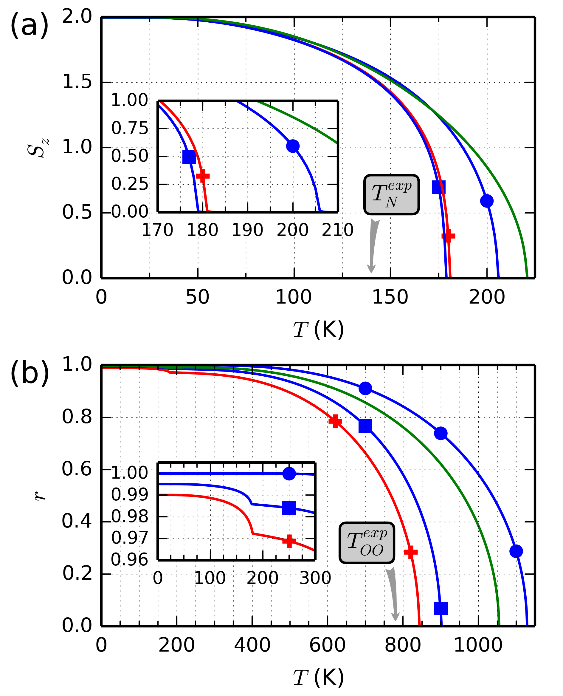
Figure 2: Temperature dependence of the on-site parameters obtained in the diverse calculation schemes: (a) spin order parameter $S^{z}$ and (b) orbital order parameter $r$. The blue and red lines with markers correspond to decoupled schemes. The temperature dependence as obtained in implementation with on-site orbital calculations (blue, bullet makers $\bullet$), the cubic cluster orbital calculations (blue, square makers $\blacksquare$), and the hedgehog cluster orbital calculations (red, $+$ makers). The green line without markers corresponds to multi-single-bond scheme. As a reference, the experimental values of phase transition temperatures are indicated in (a) and (b). Parameters as in Eqs. (16) and (17).

V.2 Spin and orbital phase transitions

For assumed physical parameters values we obtain $T^{\text{CMF}}_{\rm N}\approx 180$ K (181 K for the decoupled scheme with the hedgehog cluster). As expected, this value is higher than the experimental one ($T_{\rm N}^{\text{exp}}=140K$). The origin of the difference is in cluster MF calculation scheme. To evaluate how much the transition temperature is overestimated in MF calculation (using our sputnik cluster), we performed model cluster calculations for isotropic three-dimensional (3D) Heisenberg antiferromagnet for $S=2$ with unit magnetic exchange. One obtains the transition temperatures equal to 11.3, whereas the true value is equal to 8.5. One may deduce the latter value using the semiempirical formula Fle04 with pretty good accuracy. This means that the true transition temperature value is equal to approximately 75% of the calculated transition temperature value. In our case, we may correct the above $T^{\text{MF}}_{\rm N}\approx 180$ K using the same factor $0.75$ to obtain the corrected empirical value $T^{\text{\rm emp}}_{\rm N}\approx 135$ K. This is indeed a very good agreement with experiment.

Table 2: Orbital transition temperatures $T_{\rm OO}$ obtained in various calculation schemes. Parameters as in Eqs. (16) and (17).

calculation scheme	cluster	$T_{\rm OO}$ (K)
mean field	single site	1128
spin-orbital disentangled	hedgehog	$\,\,843$
spin-orbital disentangled	cubic	$\,\,901$
spin-orbital entangled	single bond	1055

The case of $T_{\rm OO}$ is more subtle. First we notice considerable discrepancy between the predicted values of $T_{\rm OO}$ within the various calculation schemes used, see Table 2. We adopt here the lowest value $T^{\rm CMF}_{\rm OO}=843$ K as obtained with hedgehog cluster. Note that this value is radically reduced by 25% from $T^{\rm MF}_{\rm OO}=1128$ K. As in spin case, one expects that the experimental value would be still lower but we do not have a simple method to reduce the above value to simulate the effect of quantum fluctuations in the orbital model. De facto, quantum fluctuations are much reduced in a 3D orbital system compared with the Heisenberg spin model vdB99 , so we suggest that the correction of the estimated $T^{\rm MF}_{\rm OO}$ would be less than 10% which brings it very close to experiment. This also agrees qualitatively with the expected reduction of the MF result that would be for the 3D orbital model significantly lower than 37% found for $S=1/2$ spin Heisenberg model Fle04 (which gives the corrected empirical value $T_{\rm OO}^{\rm emp}=711$ K).

Secondly we investigate the $\kappa$ dependence of $T_{\rm OO}$ (for disentangled scheme with a hedgehog cluster). We have found that $T_{\rm OO}\simeq 843$ K for $\kappa=6$ meV and $T_{\rm OO}\simeq 943$ K for $\kappa=8$ meV. This implies that in the physically interesting regime,

$$\frac{\partial T_{\rm OO}}{\partial\kappa}\simeq 50\,\frac{\rm K}{\rm meV}\,.$$ (30)

V.3 Spin exchange constants and $\big{\langle}\vec{S}_{i}\cdot\vec{S}_{j}\big{\rangle}$ correlations

In the decoupling scheme the values of $J_{\gamma}$’s constants are computed in a self-consistent way. The temperature dependence of the outcome exchange constants $J_{ab}$ and $J_{c}$ is shown in Fig. 3(a). As expected for the $A$-AF order, one finds $J_{ab}<0$ and $J_{c}>0$. The agreement with the experimental values is fair and we conclude that the overall description of the magnetic interactions in LaMnO₃ is consistent with experiment. We would like to emphasize that unlike in pure spin systems, here the exchange constants and tuned by orbital correlations and thus depend on temperature, both below and above $T_{\rm N}$. When $C$-AO exists, they are anisotropic but only below $T_{\rm N}$ the positive value of $J_{c}$ is boosted when the orbitals change below the magnetic transition. Above $T_{\rm OO}$ the spin exchange interactions are isotropic and weakly negative.

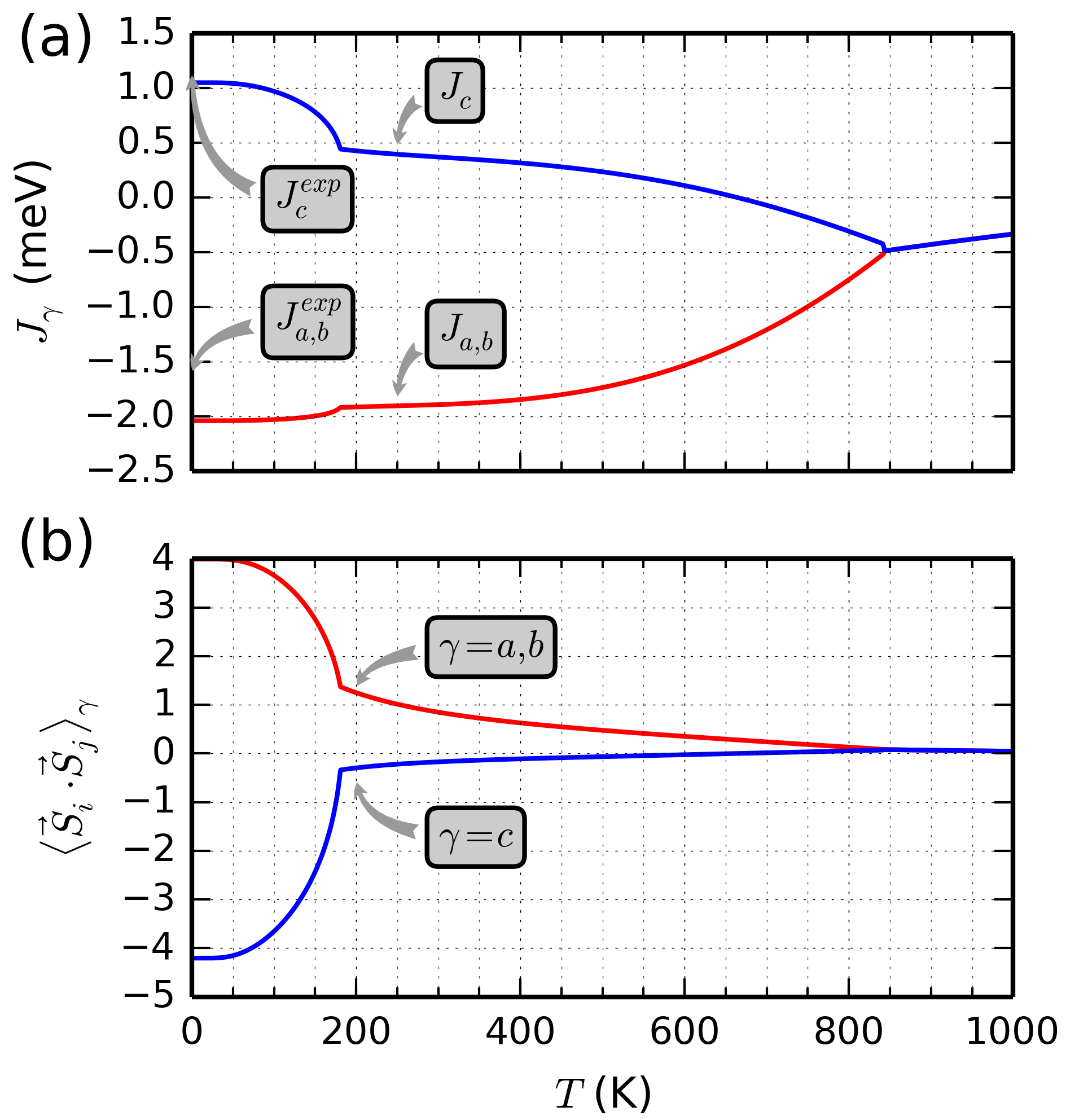
Figure 3: Temperature dependence of the effective spin model obtained from the decoupled (spin-orbital disentangled) model (in the hedgehog orbital cluster implementation): (a) spin exchange constants $J_{ab}$ and $J_{c}$ and (b) spin-spin correlations $\langle\vec{S}_{i}\cdot\vec{S}_{j}\rangle$ on nearest neighbor bonds $\langle ij\rangle$ within the $(a,b)$ planes and along the $c$ axis. Parameters as in Eqs. (16) and (17).

In a similar way the self-consistent values of spin-spin correlations for nearest neighbors, $\langle\vec{S}_{i}\cdot\vec{S}_{j}\rangle$, are obtained for $\langle ij\rangle\parallel\gamma$, for $\gamma=a,b$ and $\gamma=c$. Figure 3(b) shows the corresponding temperature dependence. Note that for $T=0$ for the bonds along the $c$ axis (the one with AF coupling $J_{c}>0$) $\langle\vec{S}_{i}\cdot\vec{S}_{j}\rangle\simeq-4.21$ which indicates some but not large quantum fluctuations. The above value belongs to the range between classical Néel value $-4.0$ and quantum singlet value for $S=2$ spins, $-6.0$. It is not surprising that due to imposed symmetry breaking the obtained value of $-4.21$ is much closer to the classical Néel state, although the quantum fluctuations are still considerable.

V.4 On-bond orbital correlations

Above $T_{rmN}$ we find $C$-AO order up to $T^{\rm CMF}_{\rm OO}$. The orbital model for $e_{g}$ orbitals is more classical than the $S=1/2$ Heisenberg model vdB99 but quantum effects are also important Ryn10 . Similar to the two-dimensional compass model where the pseudospins are entangled Cza16 , one expects that the quantum effects for $e_{g}$ orbital model contribute both to the intersite orbital correlations and to the phase transition temperature $T_{\rm OO}$. This motivates investigation of $\mathcal{P}_{\langle ij\rangle}$’s operators (4)-(6) and comparing their actual mean values with the corresponding values given by the product of MF values of $P$’s operators at sites $i$ and $j$. This study provides information about the on-bonds orbital entanglement. Here, we alias the former as true mean value and the latter as slave MF. For example, for $\mathcal{P}^{\zeta\xi}_{\langle ij\rangle}$ operator Eq. (4) one has to compare:

$$\begin{array}[]{cl}\text{mean value}&\langle\mathcal{P}^{\zeta\xi}_{\langle ij\rangle}\rangle,\\ \text{MF {Ansatz}}&2\langle P^{\zeta}_{(i}\rangle\langle P^{\xi}_{j)}\rangle.\end{array}$$

We use decoupled calculation scheme with the hedgehog orbital cluster implementation to obtain these mean values.

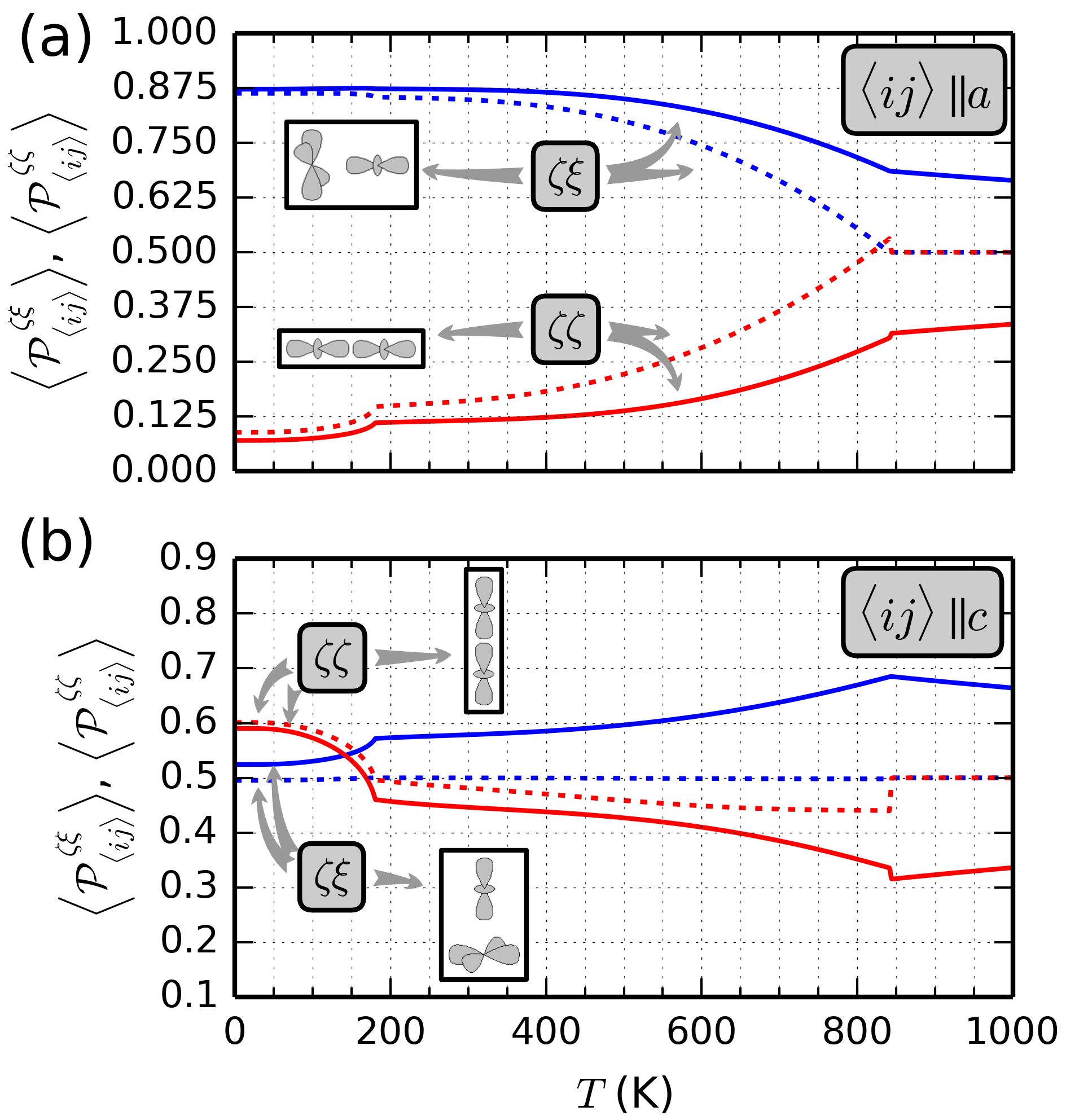
Figure 4: The true mean values: $\big{\langle}\mathcal{P}^{\zeta\xi}_{\langle ij\rangle}\big{\rangle}$ and $\big{\langle}\mathcal{P}^{\zeta\zeta}_{\langle ij\rangle}\big{\rangle}$ (solid lines) and slaves MF values: $2\big{\langle}P^{\zeta}_{(i}\big{\rangle}\langle P^{\xi}_{j)}\big{\rangle}$ and $2\big{\langle}P^{\zeta}_{i}\big{\rangle}\langle P^{\zeta}_{j}\big{\rangle}$ (dashed lines). All results are from decoupled (disentangled) calculation scheme with the hedgehog orbital cluster implementation. Parameters as in Eqs. (16) and (17).

The thermal dependence for both, the true and the factorized slave MF values of on-bound orbital projection operators, $\langle\mathcal{P}^{\zeta\zeta}_{\langle ij\rangle}\rangle$ and $\langle\mathcal{P}^{\zeta\xi}_{\langle ij\rangle}\rangle$, are shown in Fig. 4. Note, that the third on-bond orbital projection operator, $\langle\mathcal{P}^{\xi\xi}_{\langle ij\rangle}\rangle$, does not contribute to $H_{J}$ (10) and is therefore not shown.

In case of bonds parallel to the $a$ axis the most important factor that governs the $\mathcal{P}$’s operators mean values is classical correlation that follows directly from the on-site orbital pattern (with $\theta\approx 90$°). One finds that below $T_{\rm N}$ the $\mathcal{P}$’s values are close to their classical MF values ($r=1$) with $\theta=90$°. (The corresponding classical values are equal to $0.875$ and $0.125$.) In range from $T_{\rm N}$ to $T_{\rm OO}$ the parameter $r$ decreases monotonically down to $0$. The slave $\mathcal{P}$’s MF values behavior mimics this temperature dependence of the $r$ parameter. Hence slave $\mathcal{P}$’s MF values approach the high temperature limit $\frac{1}{2}$ while temperature increases $T\to T_{\rm OO}$ and take this limiting value when the orbitals are completely disordered for $T\to T_{\rm OO}$. In contrast, short-range correlations which may be seen as on-bond entanglement are enhanced near the orbital phase transition and the values of both bond projection operators, $\mathcal{P}^{\zeta\zeta}_{\langle ij\rangle\parallel ab}$ and $\mathcal{P}^{\zeta\xi}_{\langle ij\rangle\parallel ab}$ are significantly smaller/larger than $\frac{1}{2}$ for $T\approx T_{\rm OO}$. At $T_{\rm OO}$ the difference between true mean value and $\frac{1}{2}$ found in MF is approximately equal to $0.15$.

In case of bonds parallel to the $c$ axis the situation is different. Within assumed orbital pattern with $\theta\approx\pm 90$° the directional $|3z^{2}-r^{2}\rangle/\sqrt{6}$ state is just as likely as the planar $|x^{2}-y^{2}\rangle/\sqrt{2}$ state. This is the reason why the MF slave mean values of $\mathcal{P}$’s operators are here quite close to high temperature limit value $\frac{1}{2}$ (even at $T=0$). Once more, the on-bond entanglement makes the true mean value more distant from $1/2$ in comparison to slave ones. Despite that, the true mean values are quite close but deviate from $1/2$. At $T_{\rm OO}$ the difference between true mean value and $1/2$ is as big as approximately $0.20$. On-bond entanglement boosts the contribution of the configuration $|z^{2}\rangle|z^{2}\rangle$ for sites on-bond. This is reasonable, as there is an interaction $\propto\mathcal{P}^{\zeta\zeta}_{\langle ij\rangle\parallel c}$ which stabilizes this orbital configuration.

V.5 Spectral weights

A detailed experimental study of the optical spectral weights for HS and LS states was presented in Ref. Kov10 . The experimental data were obtained up to room temperature and show gradual reduction of the weight in the HS channel and an accompanying increase of the LS part for the $b$ axis polarization. For a Mott insulator the optical spectral weights can be determined from the superexchange terms $H_{J,n}^{(\gamma)}$ which stem from charge excitation $n$ to either HS or LS states along a bond in the direction $\gamma$ Kha04 . Such terms are related to the optical spectral weights via the kinetic energy,

$$K_{n}^{(\gamma)}=-2\left\langle H_{J,n}^{(\gamma)}\right\rangle.$$ (31)

These contributions depend both on the cubic direction $\gamma$ and on the type of charge transfer excitation $n$. The dimensionless optical spectral weights for HS and LS part are proportional to $K_{n}^{(\gamma)}$,

$$N_{eff}(\rm HS) = \frac{ma_{0}^{2}}{\hbar^{2}}\,K_{1}^{(\gamma)},$$ (32)

$$N_{eff}(\rm LS) = \frac{ma_{0}^{2}}{\hbar^{2}}\,\sum_{n>1}K_{n}^{(\gamma)}.$$ (33)

We used the inverse volume $a_{0}^{-3}=1.7\cdot 10^{22}$ cm^-3 Kov10 .

We present below the numerical results obtained in the entire temperature range up to the orbital transition at $T_{\rm OO}$, see Fig. 5. It is not surprising that the HS spectral weight dominates for the polarization along the $a$ axis at low temperature when $A$-AF order persists. Its decrease from $T=0$ to $T=T_{\rm N}$ is only by about 25%, and next the weight decreases steadily towards the orbital transition at $T_{\rm OO}$, see Fig. 5(a). This variation of the HS part is accompanied by gradual increase of the LS part in the entire temperature range.

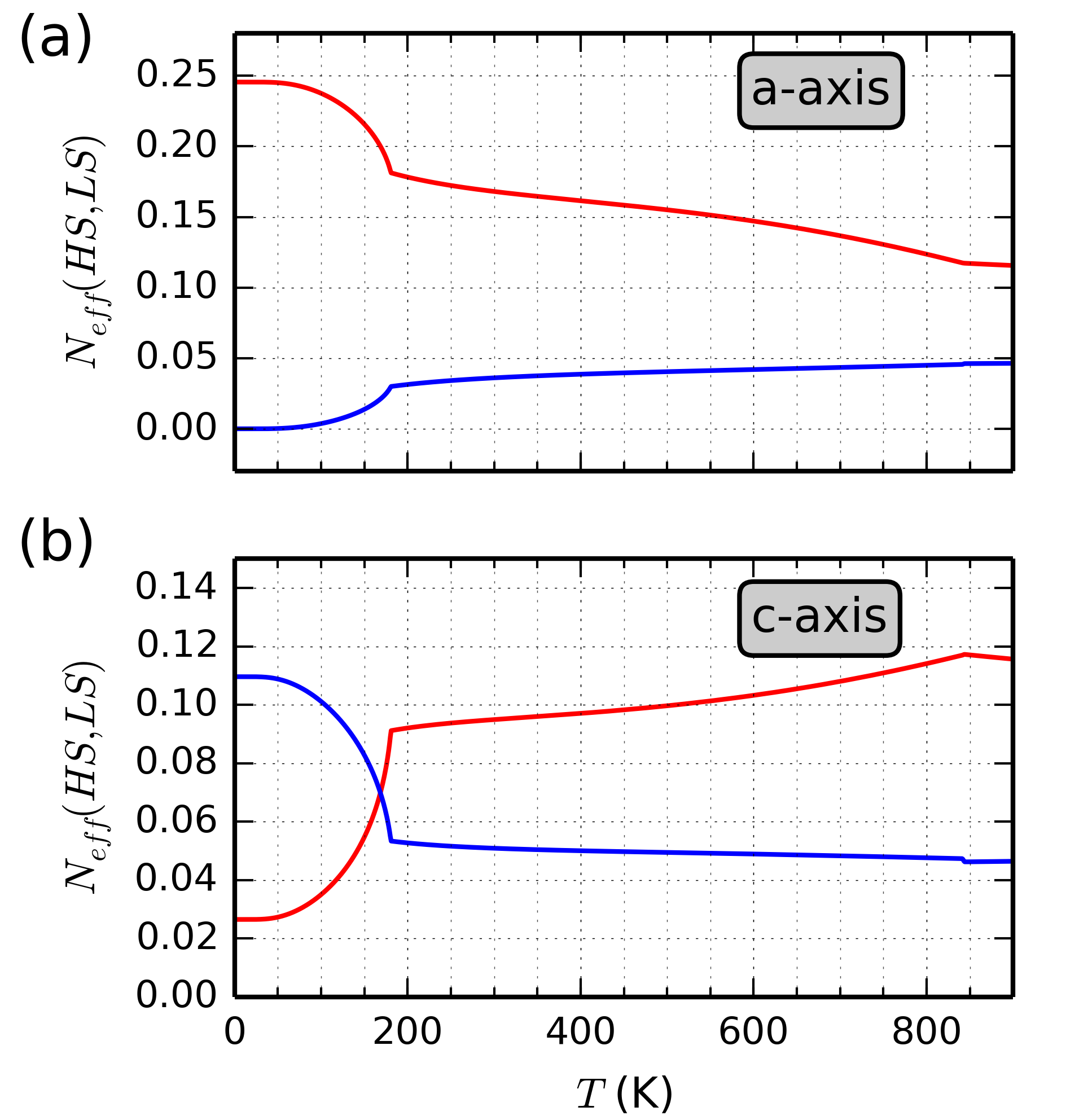
Figure 5: Optical spectral weights $N_{eff}(\rm HS)$ (red lines) and $N_{eff}(\rm LS)$ (blue lines) obtained for the polarization along the: (a) $a$ axis and (b) $c$ axis. All results are from decoupled (disentangled) calculation scheme with the hedgehog orbital cluster implementation. Parameters as in Eqs. (16) and (17).

At low temperature the role of HS and LS spectral weights is reversed for the AF bonds along the $c$ axis, see Fig. 5(b). But in contrast to the FM bonds shown in Fig. 5(a), the changes when $T_{\rm N}$ is approached from $T=0$ are here more pronounced and the LS spectral weight drops from $\sim 0.11$ at $T=0$ to $\sim 0.05$ at $T_{\rm N}$, while simultaneously the HS spectral weight increases from $\sim 0.03$ to $\sim 0.09$, i.e., by a factor close to 3. It is quite remarkable that the spectral weight for the HS part is here much higher than the that of the LS part in spite of the onset of the AF order at low temperature. We also note that the LS spectral weight practically does not change when temperature increases within the interval $T\in[T_{\rm N},T_{\rm OO}]$, and the LS weight is almost isotropic above $T_{\rm OO}$. Most importantly, we observe that: (i) the HS part dominates and is close to 0.11, while (ii) the LS part is much lower and close to 0.05 for both $a$ and $c$ bond polarization above $T_{\rm OO}$ [note different vertical scales in Figs. 5(a) and 5(b)]. Thus, the distribution of optical spectral weights becomes isotropic above $T_{\rm OO}$ and the spectral weight of the HS part is more than twice larger than that of the LS part.

VI SPIN-ORBITAL ENTANGLEMENT

VI.1 On-site spin-orbital entanglement

A fundamental problem for spin-orbital systems is weather spin and orbital operators can be disentangled, as we have implemented for all the calculations presented so far but the calculations of a single bond. Below we analyze the on-site spin-orbital entanglement in a way similar to that used for the orbital entanglement in the previous Section. We compare the calculated spin-orbital correlation, $\langle S^{z}_{i}\sigma^{z}_{i}\rangle$ with its factorized MF value, $\langle S^{z}_{i}\rangle\langle\sigma^{z}_{i}\rangle$. The results are shown in Fig. 6. Both on-site quantities are finite only below the magnetic transition at $T_{\rm N}$ and they also agree for the ground state at $T=0$.

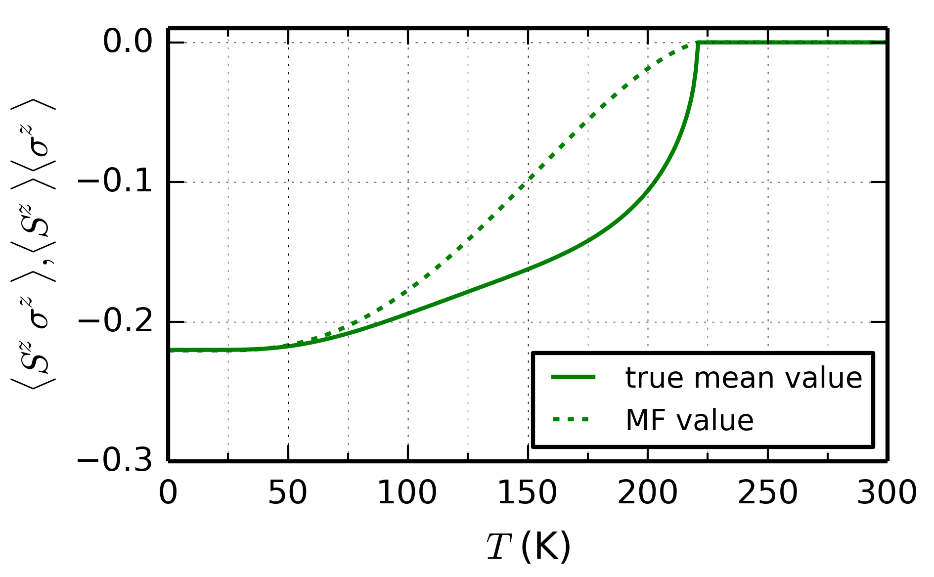
Figure 6: The calculated on-site mean value $\langle S^{z}_{i}\sigma^{z}_{i}\rangle$ (solid lines) and its MF estimated value $\langle S^{z}_{i}\rangle\langle\sigma^{z}_{i}\rangle$ (dashed lines). All results are from multi-single-bond calculation scheme, see Sec. VI.2. Parameters as in Eqs. (16) and (17).

However, one finds that some discrepancy between the actual value of $\langle S^{z}_{i}\sigma^{z}_{i}\rangle$ and its MF estimate develops in the temperature interval from approximately half of $T_{\rm N}$ to $T_{\rm N}$. This may result in some amplification of the value of $T_{\rm N}$ itself over the MF value although we should point out that the considered on-site $\langle S^{z}_{i}\sigma^{z}_{i}\rangle$ mean value may take any value from the interval $[-2.0,2.0]$ whereas it is here close to $-0.22$ at $T=0$, so we may consider it as being rather small. Furthermore, one finds that the factorized average drops faster towards zero and is already rather close to it for $T>150$ K whereas the direct calculation gives a rather different behavior, with a rapid drop of $\langle S^{z}_{i}\sigma^{z}_{i}\rangle$ close to $T_{\rm N}\simeq 220$ K.

We have also performed similar calculations for the average $|\langle S^{z}_{i}\sigma^{x}_{i}\rangle|$. Its value is much larger and close to $\sim 2.0$ at $T=0$ but one finds no discrepancy between the direct calculation and the approximate result obtained by the MF factorization here and also close to $T_{\rm N}$. Altogether we conclude that on-site spin-orbital entanglement is of little importance.

VI.2 On-bond spin-orbital entanglement

The occupied $e_{g}$ orbitals are characterized by the angle $\theta\approx 45$°, i.e., the occupied states are rather close to the eigenstates of $\sigma^{x}$ operator. Therefore, assuming that the symmetry broken states have $\langle S_{i}^{z}\rangle\neq 0$, the relevant spin-orbital correlation function, $\langle S^{z}_{i}S^{z}_{j}\sigma^{x}_{i}\sigma^{x}_{j}\rangle$, is expected to be large and negative for all the bonds. The negative value is obtained when either spins are AF and orbitals are the same for the bonds $\langle ij\rangle\parallel c$, or spins are FM but orbitals alternate in the $(a,b)$ planes for $\langle ij\rangle\parallel a$. Indeed, one finds that these mixed on-bond correlations are close to $-4.0$ independently of the bond direction, see Fig. 7. These correlation functions are almost equal to the products of spin and orbital correlations, i.e.,

$$\langle S^{z}_{i}S^{z}_{j}\sigma^{x}_{i}\sigma^{x}_{j}\rangle\simeq\langle S^{z}_{i}S^{z}_{j}\rangle\langle\sigma^{x}_{i}\sigma^{x}_{j}\rangle.$$ (34)

Therefore, spin and orbital correlations are almost disentangled.

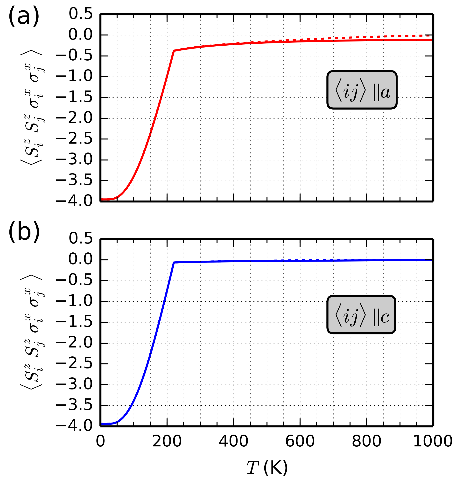
Figure 7: The calculated spin-orbital averages $\langle S^{z}_{i}S^{z}_{j}\sigma^{x}_{i}\sigma^{x}_{j}\rangle$ (solid lines) and the corresponding disentangled MF values, $\langle S^{z}_{i}S^{z}_{j}\rangle\langle\sigma^{x}_{i}\sigma^{x}_{j}\rangle$ (dashed lines) as obtained from multi-single-bond calculation scheme for a bond: (a) within the $(a,b)$ plane and (b) along the $c$ axis. Parameters as in Eqs. (16) and (17).

The on-bond spin-orbital correlations which involve $\sigma_{i}^{z}$ operators, $|\langle S^{z}_{i}S^{z}_{j}\sigma^{z}_{i}\sigma^{z}_{j}\rangle|$, are much smaller in the entire temperature range, see Fig. 8, than those involving $\sigma_{i}^{x}$, shown in Fig. 7. At $T=0$ these averages are equal to the products of spin and orbital terms, i.e., they are also disentangled. In contrast, the result obtained for $T>T_{\rm N}$ is qualitatively new. In this regime the orbital correlations $\langle\sigma^{z}_{i}\sigma^{z}_{j}\rangle$ are close to zero which explains why the MF values are almost zero for both directions, $\langle ij\rangle\parallel a$ and $\langle ij\rangle\parallel c$, see Figs. 8(a) and 8(b). This is contrast to large entanglement for $S=1/2$ spins which may trigger new phases either in the limit vanishing Hund’s exchange You15 or when spin interactions change the sign in the Kugel-Khomskii model Brz12 .

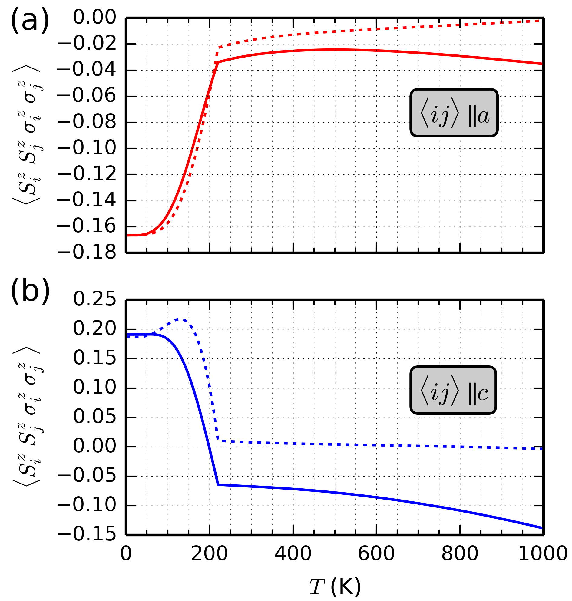
Figure 8: The calculated spin-orbital averages $\langle S^{z}_{i}S^{z}_{j}\sigma^{z}_{i}\sigma^{z}_{j}\rangle$ (solid lines) and the corresponding disentangled MF values, $\langle S^{z}_{i}S^{z}_{j}\rangle\langle\sigma^{z}_{i}\sigma^{z}_{j}\rangle$ (dashed lines) as obtained from multi-single-bond calculation scheme for a bond: (a) within the $(a,b)$ plane and (b) along the $c$ axis. Parameters as in Eqs. (16) and (17).

However, we observe that some weak spin-orbital fluctuations occur. The spin-spin correlation functions $\langle S^{z}_{i}S^{z}_{j}\rangle$, see Fig. 3(b), are much smaller than within the $A$-AF phase but are finite and follow the sign of the respective exchange constant $J_{ab}$ and $J_{c}$ above $T_{\rm N}$ — they reflect short-range spin order. Orbital order is robust and persists above $T_{\rm N}$, with $\langle\sigma^{x}_{i}\sigma^{x}_{j}\rangle\simeq\pm 1.0$ and $\langle\sigma^{z}_{i}\sigma^{z}_{j}\rangle\simeq\pm 0$, but weak spin-orbital fluctuations occur there and thus one finds for both bond directions shown in Fig. 8 that $\langle S^{z}_{i}S^{z}_{j}\sigma^{z}_{i}\sigma^{z}_{j}\rangle<0$. These finite values result from the superposition of spin short-range order with orbital thermal fluctuations. As a result the difference between the spin-orbital on-bond correlation functions and the respective products of spin and orbital MF values steadily increase above $T_{\rm N}$. Altogether we conclude that spin-orbital correlations are almost completely disentangled in the ground state but joint spin-orbital fluctuations are activated by temperature.

VI.3 The impact of entanglement on Néel temperature

The results above vividly show that, in case of finite temperature, there are some nontrivial correlations between: (i) a spin state and an orbital state at each site, and similarly (ii) orbital states of adjacent sites. Although we quantitatively describe the difference between the values of pertinent expressions of $\langle AB\rangle$ type and the corresponding expressions of $\langle A\rangle\langle B\rangle$ type, the results give us little information about the influence of corresponding correlations on the predicted magnetic transition temperature $T_{\rm N}$. As the result it is difficult to rate their physical importance.

To examine the influence of the correlations we have carried out the following numerical experiment. We involved the model in which the correlations are taken into account and calculated the value of $T_{\rm N}$ at this level of the theory. Then we modified the model in such a way that all pertinent expressions of $\langle AB\rangle$ type were changed into decoupled expressions, $\langle A\rangle\langle B\rangle$. Finally, we calculated the Néel temperature $T_{\rm N}$ in the latter model. As the only difference between the two results steams from the deliberately neglected correlation, we perceive the outgoing temperature difference as heuristic correction of $T_{\rm N}$ associated with the correlation. The relative value of the correction gives rise to a quantitative rate of the physical importance of the correlation.

For case (i) we have involved simple on-site model in which both spin and orbital degrees of freedom were introduced collectively (thus dimension of the Hilbert space is equal to 10 as it is a product of a spin quintet and an orbital doublet). Note that the model is different from the on-site model described earlier in the text (that works in decoupled calculations scheme. The site was immersed in the mean field of its surroundings (constructed in line with the $A$-AF and $C$-AO pattern). In the model values $\langle S_{z}\sigma_{z}\rangle$ occur as a part of description of the site’s surroundings. One can replace $\langle S_{z}\sigma_{z}\rangle$ by $\langle S_{z}\rangle\langle\sigma_{z}\rangle$ with ease.

For case (ii) we have involved the ”decoupled calculations” with the hedgehog orbital cluster. In this calculation values $\langle P^{\zeta_{\gamma}}_{i}P^{\zeta_{\gamma}}_{j}\rangle$ (and analogous) occur as a part of the formula for magnetic exchange constants $J_{\gamma}$, see Eq. (29). Once more, one can easily replace $\langle P^{\zeta_{\gamma}}_{i}P^{\zeta_{\gamma}}_{j}\rangle$ by the factorized product, $\langle P^{\zeta_{\gamma}}_{i}\rangle\langle P^{\zeta_{\gamma}}_{j}\rangle$.

First, for case (i) we obtained the following $T_{\rm N}$ values: 238 K for the full model and 218K for the model with the artificially broken on-site spin-orbital correlations. Of course both results are overestimated as the model consists of only one site. Nevertheless, the difference should not suffer from this problem to large extent due to the errors’ cancelation. Quite unexpectedly, the latter model has lower transition temperatures. We can elucidate this on the basis of the result presented in Fig. 6. The absolute value of $\langle S_{z}\rangle\langle\sigma_{z}\rangle$ is lower than the absolute value of $\langle S_{z}\sigma_{z}\rangle$ and hence the interaction between the site and its surroundings is weaker. It turns out, that the corresponding difference in $T_{N}$ is as big as 20K, about 10% of the total value. Second, for case (ii) we obtained the following $T_{\rm N}$ values: 181K for the full model and 201K for model with the artificially broken on-bound orbital correlations. The difference is equal to 20K.

We may conclude, that the both described correlations have significant impact on Néel temperature (close to 10% of the actual $T_{\rm N}$ value). However, corresponding corrections have opposite sign. On the grounds of this result we may draw the conclusion that the simplistic disentangled (decoupled) on-site model discussed in earlier chapters works surprisingly well as the two corrections approximately cancel out.

VII Summary and conclusions

We have investigated spin-orbital order in stoichiometric LaMnO₃ using the model reported earlier Fei99 which consists of superexchange and Jahn-Teller induced orbital terms. As a preliminary, the simple argumentation was presented that leads to quite detailed (low temperature) electronic state description. It was elucidated that the model used accounts for observed experimentally coexisting $A$-AF and $C$-AO order below the Néel temperature, and reproduces phases observed experimentally to some extent. A certain discrepancy between the predicted orbital state and the order deduced from the experimental data was detected in the value of orbital mixing angle $\theta$. Some key suggestions were given how to enrich the model — these suggestions include crystal-field effect and anharmonicity of crystal vibrations. We suggest that these extensions of the present model should be taken into account in future studies. Despite the elucidated discrepancy, for the time being, we suggest the presented analysis of electronic states within this model as insightful and instructive.

To achieve a more realistic description of the LaMnO₃ electronic state, we introduced some clusters (entities taken out of the crystal) and performed unbiased cluster mean field calculations at finite temperature. This makes, to the best of our knowledge, the first attempt to treat the spin and orbital phase transitions simultaneously in such a complex perovskite system. Cluster approach allows to evaluate the magnetic and the orbital transition temperatures in a more realistic way than within the simple on-site mean field approach. The obtained Néel temperature $T_{\rm N}\simeq 181$ K is in good agreement with experiment, taking into account the mean field nature of the cluster method.

Based on the cluster calculations the value of the effective Jahn-Teller orbital coupling constant was deduced as reproducing correctly the orbital transition temperature. Taking realistic values for all the other parameters, we find $\kappa\simeq 6$ meV in Eq. (15). Although such orbital interactions contribute on equal footing as those which result from superexchange processes for the $e_{g}$ orbital order, they are reduced from those estimated before due to the present cluster mean field approach.

By a careful analysis of entanglement, we have shown that both entangled on-site spin-orbital correlations and intersite orbital-orbital correlations influence the value of the Néel temperature $T_{\rm N}$. However, when on-site spin-orbital entanglement is included, $T_{\rm N}$ increases, while it decreases by a similar amount when intersite orbital-orbital correlations are not factorized. Therefore, the errors generated by decoupling such operators partly compensate each other which explains the apparent success of the simplified effective mean field model for LaMnO₃ where on-site spin-orbital and intersite orbital-orbital correlations are neglected.

It would be interesting to perform similar analysis of entanglement for other spin-orbital models. It is known that entanglement is large for small $S=1/2$ spins as shown for SU(2)$\otimes$SU(2) models Ole06 and for more general interactions in one dimension You15 . Here a study of spin-orbital interactions in iron pnictides Kru09 would be of interest as for $S=1$ spins one expects larger entanglement than in LaMnO₃. Experimental consequences could be quite challenging.

Finally, we emphasize that the present realistic spin-orbital superexchange model has to be treated beyond the on-site mean field to extract from it realistic values of magnetic exchange constants. The obtained values of $J_{ab}$ and $J_{c}$ explain the spin excitations in the observed $A$-type antiferromagnetic phase. We have presented also the optical spectral weights deduced from the presented model in a broad range of temperature.

Summarizing, we have shown evidence that spin-orbital entanglement is rather weak in LaMnO₃. The performed cluster mean field analysis allows us to establish that the spin-orbital entanglement is small for both on-site and on-bond quantities. This follows from large $S=2$ spins and explains why calculations based on the separation of spin and orbital degrees of freedom are so successful in providing valuable insights into the experimentally observable quantities for LaMnO₃. The most important prediction of the present theory is that the spectral weights become isotropic above the orbital transition temperature $T_{\rm OO}$ and the high-spin processes dominate over low-spin ones and give much higher spectral weight at low energy. This prediction could be of importance not only for LaMnO₃ but also for (LaNiO${}_{3})_{n}$/(LaMnO${}_{3})_{2}$ superlattices investigated recently DiP15 .

- (1) Y. Tokura and N. Nagaosa, Orbital physics in transition metal oxides, Science 288, 462 (2000).
- (2) J.-S. Zhou and J. B. Goodenough, Unusual Evolution of the Magnetic Interactions versus Structural Distortions in RMnO3 Perovskites, Phys. Rev. Lett. 96, 247202 (2006).
- (3) L. F. Feiner, A. M. Oleś, and J. Zaanen, Quantum melting of magnetic order due to orbital fluctuations, Phys. Rev. Lett. 78, 2799 (1997); Quantum disorder versus order-out-of-disorder in the Kugel-Khomskii model, J. Phys.: Condens. Matter 10, L555 (1998).
- (4) G. Khaliullin and S. Maekawa, Orbital liquid in three-dimensional Mott insulator: LaTiO3, Phys. Rev. Lett. 85, 3950 (2000).
- (5) G. Khaliullin, P. Horsch, and A. M. Oleś, Spin order due to orbital fluctuations: Cubic vanadates, Phys. Rev. Lett. 86, 3879 (2001).
- (6) G. Khaliullin, P. Horsch, and A. M. Oleś, Theory of optical spectral weights in Mott insulators with orbital degrees of freedom, Phys. Rev. B 70, 195103 (2004).
- (7) G. Khaliullin, Orbital order and fluctuations in Mott insulators, Prog. Theor. Phys. Suppl. 160, 155 (2005).
- (8) K. I. Kugel and D. I. Khomskii, The Jahn-Teller effect and magnetism: Transition metal compounds, Usp. Fiz. Nauk 136, 621 (1982) [Sov. Phys. Usp. 25, 231 (1982)].
- (9) A. M. Oleś, G. Khaliullin, P. Horsch, and L. F. Feiner, Fingerprints of spin-orbital physics in Cubic Mott insulators: Magnetic exchange interactions and optical spectral weights, Phys. Rev. B 72, 214431 (2005).
- (10) P. Horsch, A. M. Oleś, L. F. Feiner, and G. Khaliullin, Evolution of spin-orbital-lattice coupling in the VO3 perovskites, Phys. Rev. Lett. 100, 167205 (2008).
- (11) K. Wohlfeld, M. Daghofer, S. Nishimoto, G. Khaliullin, and J. van den Brink, Intrinsic Coupling of Orbital Excitations to Spin Fluctuations in Mott Insulators, Phys. Rev. Lett. 107, 147201 (2011); P. Marra, K. Wohlfeld, and J. van den Brink, Unraveling Orbital Correlations with Magnetic Resonant Inelastic X-Ray Scattering, ibid. 109, 117401 (2012); V. Bisogni, K. Wohlfeld, S. Nishimoto, C. Monney, J. Trinckauf, K. Zhou, R. Kraus, K. Koepernik, C. Sekar, V. Strocov, B. Büchner, T. Schmitt, J. van den Brink, and J. Geck, Orbital Control of Effective Dimensionality: From Spin-Orbital Fractionalization to Confinement in the Anisotropic Ladder System CaCu2O3, ibid. 114, 096402 (2015); E. M. Plotnikova, M. Daghofer, J. van den Brink, and K. Wohlfeld, Jahn-Teller Effect in Systems with Strong On-Site Spin-Orbit Coupling, ibid. 115, 106401 (2016); K. Wohlfeld, S. Nishimoto, M. W. Haverkort, and J. van den Brink, Microscopic origin of spin-orbital separation in Sr2CuO3, Phys. Rev. B 88, 195138 (2013); C.-C. Chen, M. van Veenendaal, T. P. Devereaux, and K. Wohlfeld, Fractionalization, entanglement, and separation: Understanding the collective excitations in a spin-orbital chain, ibid. 91, 165102 (2015).
- (12) W. Brzezicki, A. M. Oleś, and M. Cuoco, Spin-Orbital Order Modified by Orbital Dilution in Transition-Metal Oxides: From Spin Defects to Frustrated Spins Polarizing Host Orbitals, Phys. Rev. X 5, 011037 (2015); W. Brzezicki, M. Cuoco, and A. M. Oleś, Novel spin-orbital phases induced by orbital dilution, J. Supercond. Nov. Magn. 29, 563 (2016).
- (13) A. M. Oleś, Fingerprints of spin-orbital entanglement in transition metal oxides, J. Phys.: Condens. Matter 24, 313201 (2012); Frustration and entanglement in compass and spin-orbital models, Acta Phys. Polon. A 127, 163 (2015).
- (14) Rex Lundgren, V. Chua, and G. A. Fiete, Entanglement entropy and spectra of the one-dimensional Kugel-Khomskii model, Phys. Rev. B 86, 224422 (2012).
- (15) W.-L. You, A. M. Oleś, and P. Horsch, Entanglement driven phase transitions in spin-orbital models, New J. Phys. 17, 083009 (2015); W.-L. You, P. Horsch, and A. M. Oleś, Quantum entanglement in the one-dimensional spin-orbital SU(2)XXZ model, Phys. Rev. B 92, 054423 (2015).
- (16) S. Miyasaka, Y. Okimoto, and Y. Tokura, Anisotropy of Mott-Hubbard gap transitions due to spin and orbital ordering in LaVO3 and YVO3, J. Phys. Soc. Jpn. 71, 2086 (2002).
- (17) J. Fujioka, T. Yasue, S. Miyasaka, Y. Yamasaki, T. Arima, H. Sagayama, T. Inami, K. Ishii, and Y. Tokura, Critical competition between two distinct orbital-spin ordered states in perovskite vanadates, Phys. Rev. B 82, 144425 (2010).
- (18) E. Dagotto, T. Hotta, and A. Moreo, Colossal magnetoresistant materials: The key role of phase separation, Phys. Rep. 344, 1 (2001); E. Dagotto, Open questions in CMR manganites, relevance of clustered states and analogies with other compounds including the cuprates, New J. Phys. 7, 67 (2005).
- (19) Y. Tokura, Critical features of colossal magnetoresistive manganites, Rep. Prog. Phys. 69, 797 (2006).
- (20) Leon Balents, Spin liquids in frustrated magnets, Nature (London) 464, 199 (2010).
- (21) Lucile Savary and Leon Balents, Quantum spin liquids, arXiv:1601.03742 (2016).
- (22) L. F. Feiner and A. M. Oleś, Orbital liquid in ferromagnetic manganites: The orbital Hubbard model for eg electrons, Phys. Rev. B 71, 144422 (2005); A. M. Oleś and L. F. Feiner, Why spin excitations in ferromagnetic manganites are isotropic, ibid. 65, 052414 (2002).
- (23) B. Normand and A. M. Oleś, Frustration and entanglement in the spin-orbital model on a triangular lattice: Valence-bond and generalized liquid states, Phys. Rev. B 78, 094427 (2008); B. Normand, Multicolored quantum dimer models, resonating valence-bond states, color visons, and the triangular-lattice spin-orbital system, ibid. 83, 064413 (2011); J. Chaloupka and A. M. Oleś, Spin-orbital resonating valence bond liquid on a triangular lattice: Evidence from finite-cluster diagonalization, ibid. 83, 094406 (2011).
- (24) P. Corboz, M. Lajkó, A. M. Laüchli, K. Penc, and F. Mila, Spin-Orbital Quantum Liquid on the Honeycomb Lattice, Phys. Rev. X 2, 041013 (2012).
- (25) J. Nasu and S. Ishihara, Dynamical Jahn-Teller effect in a spin-orbital coupled system, Phys. Rev. B 88, 094408 (2013).
- (26) E. Sela, H.-C. Jiang, M. H. Gerlach, and S. Trebst, Order-by-disorder and spin-orbital liquids in a distorted Heisenberg-Kitaev model, Phys. Rev. B 90, 035113 (2014).
- (27) A. Smerald and F. Mila, Exploring the spin-orbital ground state of Ba3CuSb2O9, Phys. Rev. B 90, 094422 (2014); Disorder-Driven Spin-Orbital Liquid Behavior in the Ba3XSb2O9 Materials, Phys. Rev. Lett. 115, 147202 (2015).
- (28) F. Vernay, K. Penc, P. Fazekas, and F. Mila, Orbital degeneracy as a source of frustration in LiNiO2, Phys. Rev. B 70, 014428 (2004).
- (29) W. Brzezicki, J. Dziarmaga, and A. M. Oleś, Noncollinear magnetic order stabilized by entangled spin-orbital fluctuations, Phys. Rev. Lett. 109, 237201 (2012); Exotic Spin Orders driven by orbital fluctuations in the Kugel-Khomskii Model, Phys. Rev. B 87, 064407 (2013); Exotic spin order due to orbital fluctuations, Acta Phys. Polon. A 126, A-40 (2014).
- (30) A. Reitsma, L. F. Feiner, and A. M. Oleś, Orbital and spin physics in LiNiO2 and NaNiO2, New J. Phys. 7, 121 (2005).
- (31) J. B. Goodenough, Theory of the Role of Covalence in the Perovskite-Type Manganites [La,M(II)]MnO3, Phys. Rev. 100, 564 (1955).
- (32) D. Feinberg, P. Germain, M. Grilli, and G. Seibold, Joint superexchange-Jahn-Teller mechanism for layered antiferromagnetism in LaMnO3, Phys. Rev. B 57, R5583 (1998).
- (33) B. R. K. Nanda and S. Satpathy, Magnetic and orbital order in LaMnO3 under uniaxial strain: A model study, Phys. Rev. B 81, 174423 (2010).
- (34) N. N. Kovaleva, A. M. Oleś, A. M. Balbashov, A. Maljuk, D. N. Argyriou, G. Khaliullin, and B. Keimer, Low-energy Mott-Hubbard excitations in LaMnO3 probed by optical ellipsometry, Phys. Rev. B 81, 235130 (2010).
- (35) L. F. Feiner and A. M. Oleś, Electronic origin of magnetic and orbital ordering in insulating LaMnO3, Phys. Rev. B 59, 3295 (1999).
- (36) J. van den Brink, P. Horsch, F. Mack, and A. M. Oleś, Orbital dynamics in ferromagnetic transition metal oxides, Phys. Rev. B 59, 6795 (1999).
- (37) Eva Pavarini and Erik Koch, Origin of Jahn-Teller distortion and orbital order in LaMnO3, Phys. Rev. Lett. 104, 086402 (2010).
- (38) A. M. Oleś, L. F. Feiner, and J. Zaanen, Quantum Melting of Magnetic Long-Range Order near Orbital Degeneracy: I. Classical Phases and Gaussian Fluctuations, Phys. Rev. B 61, 6257 (2000).
- (39) B. Halperin and R. Englman, Cooperative dynamic Jahn-Teller effect. II. Crystal distortions in perovskites, Phys. Rev. B 3, 1698 (1971).
- (40) G. A. Gehring and K. A. Gehring, Co-operative Jahn-Teller effects, Rep. Prog. Phys. 38, 1 (1975).
- (41) S. Okamoto, S. Ishihara, and S. Maekawa, Orbital ordering in LaMnO3: Electron-electron and electron-lattice interactions, Phys. Rev. B 65, 144403 (2002).
- (42) O. Sikora and A. M. Oleś, Origin of the Orbital Ordering in LaMnO3, Acta Phys. Polon. B 34, 861 (2003).
- (43) Q. Huang, A. Santoro, J. W. Lynn, R. W. Erwin, J. A. Borchers, J. L. Peng, and R. L. Greene, Structure and magnetic order in undoped lanthanum manganite, Phys. Rev. B 55, 14987 (1997).
- (44) A. F. Albuquerque, D. Schwandt, B. Hetényi, S. Capponi, M. Mambrini, and A. M. Läuchli, Phase diagram of a frustrated quantum antiferromagnet on the honeycomb lattice: Magnetic order versus valence-bond crystal formation, Phys. Rev. B 84, 024406 (2011).
- (45) D. Gotfryd, J. Rusnačko, K. Wohlfeld, G. Jackeli, J. Chaloupka, and A. M. Oleś, Phase diagram and spin correlations of the Kitaev-Heisenberg model: Importance of quantum effects, arXiv:1608.05333 (2016).
- (46) This formula is based on experimental data and was introduced by G. S. Rushbrooke and P. J. Wood, Mol. Phys. 1, 257 (1958); see also: M. Fleck, A. I. Lichtenstein, M. G. Zacher, W. Hanke, and A. M. Oleś, On the nature of the magnetic transition in a Mott insulator, Eur. Phys. J. B 37, 439 (2004).
- (47) A. van Rynbach, S. Todo, and S. Trebst, Orbital Ordering in Orbital Systems: Ground States and Thermodynamics of the 120° Model, Phys. Rev. Lett. 105, 146402 (2010).
- (48) P. Czarnik, J. Dziarmaga, and A. M. Oleś, Variational tensor network renormalization in imaginary time: Two-dimensional quantum compass model at finite temperature, Phys. Rev. B 93, 184410 (2016).
- (49) A. M. Oleś, P. Horsch, L. F. Feiner, and G. Khaliullin, Spin-Orbital Entanglement and Violation of the Goodenough-Kanamori Rules, Phys. Rev. Lett. 96, 147205 (2006).
- (50) F. Krüger, S. Kumar, J. Zaanen, and J. van den Brink, Spin-orbital frustrations and anomalous metallic state in iron-pnictide superconductors, Phys. Rev. B 79, 054504 (2009).
- (51) P. Di Pietro, J. Hoffman, A. Bhattacharya, S. Lupi, and A. Perucchi, Spectral Weight Redistribution in (LaNiO/(LaMnO Superlattices from Optical Spectroscopy, Phys. Rev. Lett. 114, 156801 (2015).