Green’s function variational approach to orbital polarons in KCuF₃

Abstract

We develop an $e_{g}$ orbital, $t$-$J$-like model of a single charge doped into a two-dimensional plane with ferromagnetic spin order and alternating orbital order, and present its solution by Green’s functions in the variational approximation framework. The model is designed to represent the orbital physics within ferromagnetic $(a,b)$ planes of KCuF₃ and K₂CuF₄. The variational approximation (VA) relies on the systematic generation of equations of motion for the Green’s function, taking into account the real-space constraints coming from the exclusion of doubly occupied sites. This method is compared to the firmly established self-consistent Born approximation, and to the variational cluster approximation (VCA) which relies on the itinerant regime of the model. We find that the present variational approximation captures the essential aspects of the spectral weight distribution of the coherent quasiparticle state and gives a result similar to the VCA, while also reproducing well the momentum dependence of the spectral moments. In contrast, the spectral function obtained within the self-consistent Born approximation is more incoherent and its quasiparticle is heavier, at strong effective couplings, than observed with VCA and VA.

I Introduction

Strongly correlated electron systems with active orbital degrees of freedom pose a variety of challenging problems. One of them is charge propagation in systems with orbital order which has a whole plethora of possible processes involving the ordered background Zaanen and Oleś (1993). Some of them could support coherent hole propagation, but in general the charge is expected to be confined when the spin-orbital order is robust Wohlfeld et al. (2009). This problem simplifies tremendously when the orbital degrees of freedom are quenched, as in high $T_{c}$ superconducting cuprates, and hole propagation in the antiferromagnetic (AF) background may be studied for a two-dimensional (2D) square lattice Lee et al. (2006) within the effective $t$-$J$ model or its extensions Tohyama and Maekawa (1994); *Bal95. In these systems individual CuO₂ planes are separated from one another and it is sufficient to investigate charge propagation within a single plane. A hole added to a quantum antiferromagnet propagates then by processes which involve quantum fluctuations in the spin background and this propagation is controlled by a new energy scale set by the superexchange $J$ Martínez and Horsch (1991). In contrast, a hole is almost blocked in the absence of quantum fluctuations for Ising exchange interactions — then the hopping in a square lattice is possible only by self-repairing processes on plaquettes, as recognized by Trugman Trugman (1988).

In this context the orbital models are of particular interest as they offer several different scenarios as the exchange interactions are always of lower symmetry than SU(2) and also the orbital flavor is not conserved in some cases. They originate from the spin-orbital physics Kugel and Khomskii (1982); Feiner et al. (1997); *Fei98; Feiner and Oleś (1999); Khaliullin and Maekawa (2000); Khaliullin et al. (2001); *Kha04; Oleś et al. (2005); Khaliullin (2005); Reitsma et al. (2005); Cuoco et al. (2006); Chaloupka and Khaliullin (2008); Krüger et al. (2009); Corboz et al. (2012); Brzezicki et al. (2012); *Brz13; *Brz11; *Cza15; Wohlfeld et al. (2011); *Mar12; *Bis15; *Plo16; *Woh13; *Che15; Brzezicki et al. (2014a); Smerald and Mila (2014); Avella et al. (2015); *Hor11; *Ave13; Kat15; Brzezicki et al. (2015a); *Brzjs, and arise when spin order is ferromagnetic (FM) — then the superexchange reduces to orbital interactions only and spin-orbital entanglement Oleś (2012); *Ole15 is absent in the ground state Oleś et al. (2006); You et al. (2015a); *You12; *Hor15. Realistic 2D or three-dimensional (3D) $e_{g}$ orbital models are also strongly frustrated, but nevertheless alternating orbital (AO) order arises at finite temperature and is induced by the strongest interaction van Rynbach et al. (2010), while quantum effects are small van den Brink et al. (1999). Doping of the $e_{g}$ orbital system suppresses gradually orbital order Tanaka et al. (2005); *Tan09 and gives a disordered orbital liquid which plays a role in doped FM manganites Feiner and Oleś (2005). It was argued that orbital non-conserving processes (see below) are responsible for the onset of the disordered orbital liquid for larger doping. Indeed, such a disordered orbital state supports the FM metallic phase in doped manganites and was invoked to explain the observed cubic symmetry in the 3D magnon dispersion for La_1-xPb_xMnO₃ Khaliullin and Kilian (2000); *Ole02.

Concerning the hole propagation, it is important to realize that the orbital models are more classical than spin ones, for instance the orbital model for $t_{2g}$ orbitals has Ising superexchange and thus realizes the paradigm introduced by Trugman Trugman (1988). One expects that in absence of orbital fluctuations holes should be immobile. Yet, weak hole propagation becomes possible due to three-site processes for $t_{2g}$ orbitals, which appear in doped systems in the same order of the perturbation theory as the superexchange itself Daghofer et al. (2008); *Woh08; Wróbel and Oleś (2010). The three-site terms dominate also hole propagation in the 2D compass model Brzezicki et al. (2014b); *Dag15 which is related to the $e_{g}$ orbital model Cincio et al. (2010). Finally, recently it was argued that the concept of hole-localization in the absence of quantum fluctuations does not to apply to three-band models Ebrahimnejad et al. (2014, ).

Perhaps the most complex situation arises in the $e_{g}$ orbital model where both the orbital superexchange interactions van den Brink et al. (1999) and the kinetic energy Feiner and Oleś (2005) are radically different from their counterparts in the spin $t$-$J$ model. The interactions are Ising-like in a one-dimensional (1D) model Daghofer et al. (2004) and involve one directional ($3z^{2}-r^{2}$)-like orbital and one perpendicular to it ($x^{2}-y^{2}$)-like orbital, both selected by the bond direction. Therefore, the 1D orbital model is classical but quantum fluctuations increase with increasing dimension: the 2D model and even more so the 3D model become quantum, but still both have much weaker quantum fluctuations van den Brink et al. (1999) than the SU(2) symmetric Heisenberg spin model.

In addition, the hopping in dimension higher than one does not conserve the orbital flavor and includes both the intraorbital processes with and interorbital ones without orbital conservation Feiner and Oleś (2005). The orbital-flip processes allow an alternative mode of hole propagation, where the orbital order of the ground state is not disturbed at all. As the hole thus needs neither spin-flip nor three-site terms to move, one would expect to observe a quasiparticle (QP) dispersion on a scale of the (interorbital) hopping $t$ rather than on the scale of $J$. The additional presence of orbital-flipping hoppings mediates interactions with the background that can further renormalize the bandwidth, however the extremely small dispersion found with the self-consistent Born approximation (SCBA) Martínez and Horsch (1991) comes as a surprise and seems to contradict this picture van den Brink et al. (2000).

The purpose of this paper is to present a systematic study of hole propagation in the 2D $e_{g}$ orbital model. A full understanding of this orbital-polaron is a necessary ingredient – together with the full understanding of the spin-polaron – before one can hope to understand the complex behavior of spin-orbital polarons, i.e., of the QPs that form in systems with strong coupling to both orbital and spin excitations Wohlfeld et al. (2009).

To study the polaron of the 2D $e_{g}$ orbital model, we go beyond the simplest SCBA approach and also investigate the consequences of the local real space constraints on the hole propagation. By comparing with the variational approach, we establish that the SCBA, which includes only rainbow diagrams, gives a surprisingly good qualitative picture. However, we also find that its one weakness is that it gives predominantly incoherent spectra with too small QP bandwidth. Indeed, we find that the other approaches yield a fairly robust dispersion, which is more easily reconciled with the underlying propagation mechanism. We also develop and validate a variational approach to the problem that can more easily be generalized to the full 3D model.

The paper is organized as follows: In Sec. II we introduce the $e_{g}$ orbital Hamiltonian for a 2D $(a,b)$ plane and identify the processes responsible for free hole propagation as well as interactions which will have to be treated by some approximate method. In this paper we employ several methods introduced in Sec. III: (i) variational approach in Sec. III.1, (ii) self-consistent Born approximation (SCBA) in Sec. III.2, (iii) variational cluster approximation (VCA) in Sec. III.3, and (iv) spectral moment approach in Sec. III.4. We then discuss the convergence of the variational approach upon increasing the variational space, and present and compare with one another the numerical results obtained using these various methods in Sec. IV. The summary and conclusions are given in Sec. V. The paper is completed by Appendix A which elaborates on the details of the variational solution.

II The 2D orbital model

KCuF₃ is a 3D perovskite material, with staggered FM $(a,b)$ planes along the $c$ cubic axis Lake et al. (2005). Each $(a,b)$ plane has AO order following the Goodenough-Kanamori rules Goode; Kan59. A carrier doped into this material will couple to both spin and orbital excitations to realize its motion Wohlfeld et al. (2009). As already mentioned, our current goal is to understand the orbital-polaron that forms when the carrier is restricted to move within a single $(a,b)$ plane. The spin degree of freedom is then quenched and only orbital interactions survive.

To address this situation we start with the on-site Coulomb interactions for two degenerate $e_{g}$ orbitals $\{z,\bar{z}\}$ at Cu sites; they read Ole83,

$$H_{\mathrm{int}} =U_{0}\sum_{i,\mu=z,\bar{z}}n_{i\mu,\uparrow}n_{i\mu,\downarrow}$$

$$+\sum_{i}\left(U_{0}-\frac{5}{2}J_{\mathrm{H}}\right)n_{iz}n_{i\bar{z}}-2J_{\mathrm{H}}\sum_{i}\mathbf{S}_{iz}\cdot\mathbf{S}_{i\bar{z}}$$ (1)

$$+J_{\mathrm{H}}\sum_{i}\left(d^{\dagger}_{iz,\uparrow}d^{\dagger}_{iz,\downarrow}d_{i\bar{z},\downarrow}d_{i\bar{z},\uparrow}+d^{\dagger}_{i\bar{z},\uparrow}d^{\dagger}_{i\bar{z},\downarrow}d_{iz,\downarrow}d_{iz,\uparrow}\right).$$

The basis $\{z,\bar{z}\}$ was chosen as consisting of one directional $z$ orbital along the cubic $c$ axis, and orthogonal to it $\bar{z}$ orbital within the $(a,b)$ plane as follows:

$$\begin{split}\lvert z\rangle&\equiv\lvert 3z^{2}-r^{2}\rangle/\sqrt{6},\\ \lvert\bar{z}\rangle&\equiv\lvert x^{2}-y^{2}\rangle/\sqrt{2}.\end{split}$$ (2)

The interactions in Eq. (II) are parametrized by two parameters: intraorbital Coulomb element $U_{0}$ and Hund’s exchange $J_{\mathrm{H}}$. These parameters decide about the energies of the ground and excited states. In the present case of Cu²⁺ ions with $d^{9}$ configuration, $H_{\mathrm{int}}$ does not contribute to the ground states of a single hole at each site.

Among the excited states at Cu³⁺ ions with $d^{8}$ ($t_{2g}^{6}e_{g}^{2}$) configurations, the high-spin $S=1$ states, as for instance $|z\!\uparrow\bar{z}\!\uparrow\rangle$, have the lowest energy of $(U_{0}-3J_{H})$ Oleś et al. (2005). These states with two holes occupying two orthogonal orbitals of $d^{8}$ ions arise by charge excitations on the bonds within the $(a,b)$ planes of KCuF₃ and decide about the FM order. Thus, as long as we limit ourselves to a single FM plane, we can consider spinless $d^{\dagger}_{i\mu,\uparrow}\equiv d^{\dagger}_{i\mu}$ fermions and replace Eq. (II) with

$$\mathcal{H}_{U}=U\sum_{i}n_{iz}n_{i\bar{z}},$$ (3)

where the effective interaction between two holes with different orbital flavors at the same site $i$ is,

$$U\equiv U_{0}-3J_{H}.$$ (4)

Thus, from now on the effective parameter $U$ stands for the interaction $(U_{0}-3J_{H})$ which is the only interaction left in the subspace of high-spin (triplet) excited states van den Brink et al. (1999).

We supplement the above interaction term with the kinetic energy for $e_{g}$ spinless holes on the full 3D lattice assuming FM order Feiner and Oleś (2005):

$$\mathcal{H}_{t}=-t\sum_{\alpha}\sum_{\langle ij\rangle\|\alpha}\left(d_{iz_{\alpha}}^{{\dagger}}d_{jz_{\alpha}}+\mathrm{H.c.}\right),$$ (5)

which describes the hopping between nearest neighbor (NN) sites along each bond $\langle ij\rangle$ that involves two $\sigma$-bonding $\lvert 3z_{\alpha}^{2}-r^{2}\rangle$-type orbitals oriented along the bond direction $\alpha=\{a,b,c\}$, with $z_{c}\equiv z$, etc. As the hopping $t$ follows from a two-step process via ligand F($2p$) orbitals, the $\delta$-hopping between two $\lvert x_{\alpha}^{2}-y_{\alpha}^{2}\rangle$-type orbitals, which are perpendicular to the direction $\alpha$, vanishes by symmetry. We use again the same short-hand notation with $x_{c}\equiv x$, $y_{c}\equiv y$, etc. The above formulation, while concise, is not very practical due to the orbital basis changing depending on the $\alpha$ direction. By transforming the Hamiltonian (5) to the standard orthogonal orbital basis (2) one obtains:

$$\mathcal{H}_{t}=-t\sum_{\langle ij\rangle\|c}d_{iz}^{{\dagger}}d_{jz}\\ -\frac{t}{4}\sum_{\langle ij\rangle\|a}\left[(d_{iz}^{{\dagger}}-\sqrt{3}d_{i\bar{z}}^{{\dagger}})(d_{jz}-\sqrt{3}d_{j\bar{z}})+\mathrm{H.c.}\right]\\ -\frac{t}{4}\sum_{\langle ij\rangle\|b}\left[(d_{iz}^{{\dagger}}+\sqrt{3}d_{i\bar{z}}^{{\dagger}})(d_{jz}+\sqrt{3}d_{j\bar{z}})+\mathrm{H.c.}\right].$$ (6)

The results presented below are in units of $t=1$.

Here we are interested both in the orbital Hubbard model for $e_{g}$ electrons/holes Feiner and Oleś (2005) given by Eqs. (3) and (6), and in effective large-$U$ models, i.e., superexchange models derived by second-order perturbation expansion of the Hamiltonian. Following a procedure analogous to the $t$-$J$ model derivation Cha77, one can find the exchange interaction, which in this case consists of four terms expressed using singlet/triplet projection operators in spin and orbital Hilbert spaces.

Although in KCuF₃ the spin interactions in $(a,b)$ planes are rather weak, the ground state has $A$-type AF spin and $C$-type AO order Paolasini et al. (2002); *Bella, i.e., we can view the system as consisting of strongly coupled $(a,b)$ planes with AO order that are stacked with ferro-orbital (FO) order along the $c$ axis. AF correlations between the layers strongly suppress hole motion in $c$ direction, making it feasible to focus on the in-plane orbital physics separately from the system’s behavior along the $c$-direction, at least as long as we are considering a system near its ground state.

To find the exchange Hamiltonian for a single 2D plane we need to project out the spin-singlet states from the full Hamiltonian. After averaging over the in-plane spin-triplet states one arrives at van den Brink et al. (1999):

$$\mathcal{H}_{J}=\frac{J}{2}\sum_{\langle ij\rangle}[T_{i}^{z}T_{j}^{z}+3T_{i}^{x}T_{j}^{x}\mp\sqrt{3}(T_{i}^{x}T_{j}^{z}+T_{i}^{z}T_{j}^{x})],$$ (7)

where $J=t^{2}/U$, the upper/lower sign is for the $\langle ij\rangle$ bond oriented along $a/b$ axis respectively, and $\{T_{i}^{\alpha}\}$ operators are the same as spin operators (1/2 times the respective Pauli matrix), only acting in the orbital space in which $z/\bar{z}$ states correspond to spin up/down states. Alternatively, one may derive Eq. (7) from the Kugel-Khomskii model Kugel and Khomskii (1982); Feiner et al. (1997) by considering a FM system with superexchange given by triplet charge excitations $d_{i}^{9}d_{j}^{9}\leftrightarrow d_{i}^{8}d_{j}^{10}$.

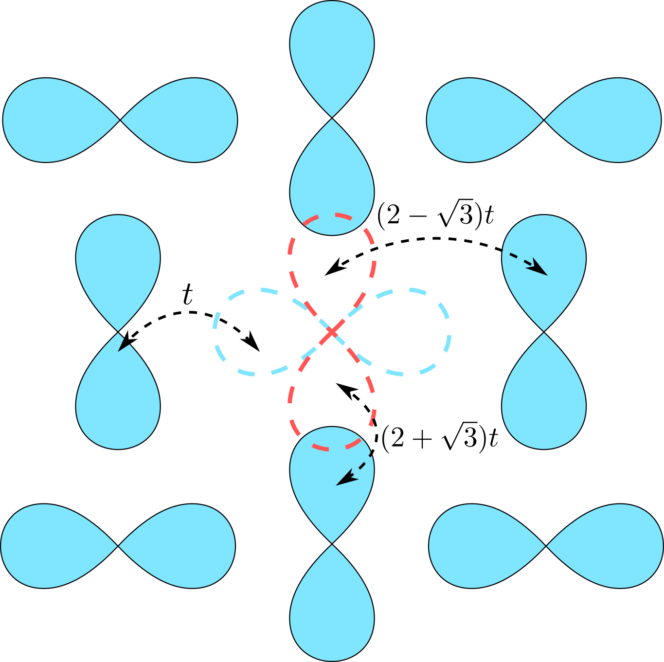
Figure 1: (Color online) Schematic representation of the kinetic Hamiltonian $\mathcal{H}_{t}$ (6) and the ground state with AO order of the 2D orbital model $\mathcal{H}_{J}$ (7). The bow-shapes represent the $\lvert\pm\rangle$ states which are highly directional in the $(a,b)$ plane. Full orbitals represent a singly occupied state (corresponding to the overall $d^{9}$ state) and the blue color represents the orbitals occupied in the ground state. The dashed orbital contours represent a doubly occupied central site (i.e., electron doping). Blue contour refers to the orbital normally half-filled in the ground state and the red one indicates the orbital that would have been wrongly occupied if an electron were to be removed from it. The kinetic elements of Hamiltonian (11) are a consequence of orbital symmetry and overlap.

For an FM plane in KCuF₃, or for the 2D compound K₂CuF₄, it has been well established through a variety of analytical and numerical treatments van den Brink et al. (1999); Cincio et al. (2010); vdB04; Daghofer et al. (2006) that the leading superexchange term $3T^{x}_{i}T^{x}_{j}$ dominates Eq. (7) and stabilizes the AO order shown schematically in Fig. 1. Indeed, the orbital ground state has been found to be composed of alternating eigenstates of $T^{x}$ operators, i.e.,

$$\lvert\pm\rangle=\frac{1}{\sqrt{2}}(\lvert z\rangle\pm\lvert\bar{z}\rangle).$$ (8)

Orbital excitations from such an ordered ground state have been studied by several authors in the past van den Brink et al. (1999); Wohlfeld et al. (2011); *Mar12; *Bis15; *Plo16; *Woh13; *Che15; Oka02; Ish05; For08; Nas13. Below we use them to investigate orbital polarons when a hole is added.

Quantum fluctuations around perfect Néel order involve one- and two-orbiton (orbital excitation) processes and have consistently been found to be small. As a further check, we carried out the SCBA with and without these quantum fluctuations and have found the results to be almost identical. Thus, while the other two terms can be included in the treatment (they are automatically included in the VCA) in the following we restrict the variational approach to only the Ising-exchange term $\mathcal{H}_{J}\approx\frac{3}{2}J\sum_{\langle ij\rangle}T^{x}_{i}T^{x}_{j}$, for the sake of simplicity.

The kinetic Hamiltonian (6), after being restricted to the $(a,b)$ plane, is transformed to the basis (8). Next, the orbital degree of freedom is decoupled from the fermionic operators by means of the slave boson formalism Martínez and Horsch (1991):

$$d_{i0}^{{\dagger}}=f_{i}^{{\dagger}},\quad d_{i1}^{{\dagger}}=f_{i}^{{\dagger}}a_{i},$$ (9)

where the $\{0,1\}$ indices on the left hand side indicate fermion creation in the ground or excited state, respectively, i.e., $\lvert+\rangle$ or $\lvert-\rangle$ (8), depending on the sublattice since the orbital state is alternating. This transformation works under the assumption that $f_{i}^{{\dagger}}:d^{9}\to d^{10}$ and $f_{i}:d^{10}\to d^{9}$, which is the consequence of disallowing doubly occupied states in the Hilbert space.

After performing all the above transformations, we arrive at the final form of the strong coupling Hamiltonian,

$$\mathcal{H}=\mathcal{H}_{J}+\mathcal{T}+\mathcal{V},$$ (10)

where:

$$\mathcal{H}_{J} =\frac{3}{8}J\sum_{\langle ij\rangle}(1-\sigma_{i}^{z}\sigma_{j}^{z}),$$ (11a)

$$\mathcal{T} =-\frac{t}{4}\sum_{\langle ij\rangle}(f_{i}^{{\dagger}}f_{j}+\mathrm{H.c.})=\sum_{\mathbf{k}}\epsilon_{\mathbf{k}}f_{\mathbf{k}}^{{\dagger}}f_{\mathbf{k}},$$ (11b)

$$\mathcal{V} =-\frac{t}{4}\sum_{i,\delta}\left[(2+\sqrt{3}e^{i\pi_{y}\cdot\delta}e^{i\mathbf{Q}\cdot\mathbf{R}_{i}})a_{i}^{{\dagger}}+\right.$$

$$\left.+(2-\sqrt{3}e^{i\pi_{y}\cdot\delta}e^{i\mathbf{Q}\cdot\mathbf{R}_{i}})a_{i+\delta}+a_{i}^{{\dagger}}a_{i+\delta}\right]f_{i+\delta}^{{\dagger}}f_{i}.$$ (11c)

Here, $\epsilon_{\mathbf{k}}=-t\gamma_{\mathbf{k}}$ is the free particle dispersion, with $\gamma_{\mathbf{k}}=(1/z)\sum_{\delta}e^{i\mathbf{k}\cdot\delta}$. Also, for simplicity $\mathcal{H}_{J}$ and the corresponding ground state have been transformed from AO order into the FO one, and the leading Ising term has the exchange constant $J$ with an explicit factor of $-3/8$. Note that we also subtracted the background energy out of $\mathcal{H}_{J}$. The free propagation $\mathcal{T}$ (11b) is the consequence of the kinetic energy terms conserving the orbital flavor, while the interaction $\mathcal{V}$ (11) arises by the same mechanism as the hole-magnon coupling in the spin model Martínez and Horsch (1991). The phase factors serve to accommodate the model’s dependence on direction: $\pi_{y}=(0,\pi)$, $\mathbf{Q}=(\pi,\pi)$, and $\delta$ is a vector variable pointing to the nearest neighbors of site $i$.

III Methods

III.1 Variational approximation (VA)

Starting from the Bloch state of a free electron,

$$\lvert\mathbf{k}\rangle=f_{\mathbf{k}}^{{\dagger}}\lvert 0\rangle=\frac{1}{\sqrt{N}}\sum_{i}e^{i\mathbf{k}\cdot\mathbf{R}_{i}}f_{i}^{{\dagger}}\lvert 0\rangle,$$ (12)

we define the Green’s function as

$$G(\mathbf{k},\omega)\equiv\langle\mathbf{k}\rvert\mathcal{G}(\omega)\lvert\mathbf{k}\rangle,$$ (13)

where $\mathcal{G}(\omega)=(\omega+i\eta-\mathcal{H})^{-1}$ is the resolvent. Here, $|0\rangle$ is the Néel AO ground-state of the undoped 2D plane, described above.

The variational approximation is based on a simplification of the equations of motion which are obtained through repeated Dyson expansions of the resolvent:

$$\mathcal{G}(\omega)=\mathcal{G}_{0}(\omega)+\mathcal{G}(\omega)\mathcal{V}\mathcal{G}_{0}(\omega).$$ (14)

Here, $\mathcal{H}_{0}=\mathcal{T}+\mathcal{H}_{J}$ corresponds to $\mathcal{G}_{0}(\omega)$ and $\mathcal{V}$ is given by Eq. (11).

The rationale underlying the variational approach is that the creation of every orbiton costs an energy proportional to $J$, so the bigger the value of $J$ the less orbitons are likely to appear in the QP cloud in the ground state. Therefore, one can restrict the Dyson expansion in terms of the number of orbitons generated in the system, and one can further decrease the Hilbert space by constraining the orbitons to be located close to each other. This approach can of course be tested by verifying the convergence of the result as a function of the number of orbitons allowed in the system, i.e., by increasing the variational space. In this Section we show how this approach works in the framework of a one orbiton approximation, when only up to one orbiton is allowed to appear in the QP cloud. Then we briefly discuss the generalization for the two-orbiton case, which is further detailed in the Appendix. Note that we have implemented this variational approach, and show results, for up to six orbitons in the QP cloud. However, those equations of motion become too cumbersome to write explicitly. We also note that similar variational schemes have proved to be very accurate for the study of various models of lattice polarons Berciu (2006); Goodvin et al. (2006); Berciu (2007); Marchand et al. (2010) as well as spin polarons Berciu and Fehske (2011); Trousselet et al. (2013); Ebrahimnejad et al. (2014, ).

Using the Dyson expansion and evaluating $\mathcal{V}\lvert\mathbf{k}\rangle$ explicitly in real space, we arrive at the following expression:

$$\begin{split}&G(\mathbf{k},\omega)=\left[1-\frac{t}{2}\sum_{\delta}F_{1}(\mathbf{k},\omega,\delta)+\right.\\ &\left.-\frac{\sqrt{3}t}{4}\sum_{\delta}\bar{F}_{1}(\mathbf{k},\omega,\delta)e^{i\mathbf{\pi}_{y}\cdot\mathbf{\delta}}\right]G_{0}(\mathbf{k},\omega-4J^{\prime}),\end{split}$$ (15)

where $G_{0}((\mathbf{k},\omega)=(\omega-\epsilon_{\mathbf{k}}+i\eta)^{-1}$ is the free-electron Green’s function, the shorthand notation $J^{\prime}=3J/8$ has been introduced for convenience, and we define:

$$F_{1}(\mathbf{k},\omega,\delta) =\langle\mathbf{k}\rvert\mathcal{G}(\omega)\frac{1}{\sqrt{N}}\sum_{i}e^{i\mathbf{k}\cdot\mathbf{R}_{i}}f_{i+\delta}^{{\dagger}}a_{i}^{{\dagger}}\lvert 0\rangle,$$ (16)

$$\bar{F}_{1}(\mathbf{k},\omega,\delta) =\langle\mathbf{k}\rvert\mathcal{G}(\omega)\frac{1}{\sqrt{N}}\sum_{i}e^{i(\mathbf{k+Q})\cdot\mathbf{R}_{i}}f_{i+\delta}^{{\dagger}}a_{i}^{{\dagger}}\lvert 0\rangle,$$ (17)

as the generalized Green’s functions for the state with a single orbital excitation above the ground state.

In order to find these new propagators, we use the Dyson expansion again to generate their equations of motion. In the one-orbiton variational scheme we include only the part of $\mathcal{V}$ which does not create new orbitons. However, at this point one has to impose additional constraints on the movement of the electron, namely: ($i$) the electron and the orbiton cannot both occupy the same site, and ($ii$) when the electron and orbiton are far apart the energy increase is by $12J^{\prime}$ (4 broken bonds accompanied by 4 excited bonds), however if they are on adjacent sites the energy increase is only by $10J^{\prime}$ (one excited bond less). The above constraints can be taken into account by adding the following terms to the $\mathcal{H}_{0}$ Hamiltonian, in order to cancel the corresponding processes:

$$\mathcal{V}_{1}=\frac{t}{4}\sum_{\epsilon}(f_{i}^{{\dagger}}f_{i+\epsilon}+\mathrm{H.c.})-2J^{\prime}\sum_{\epsilon}n_{i+\epsilon},$$ (18)

where $i$ is the location of the orbiton and $n_{i+\epsilon}$ is the electron number operator for the sites NN to site $i$. The above expression modifies the free part of the Hamiltonian, which means now instead of $\mathcal{G}_{0}(\omega)$ one has to use $\mathcal{G}_{1}(\omega)$ (corresponding to $\mathcal{H}_{0}+\mathcal{V}_{1}$) in the Dyson expansion of the generalized Green’s function:

$$\mathcal{G}(\omega)=[1+\mathcal{G}(\omega)\mathcal{V}]\mathcal{G}_{1}(\omega).$$ (19)

However, $\mathcal{G}_{1}(\omega)$ is no longer diagonal in Fourier space, and so its propagator needs to be solved first. This can again be done using the Dyson equation,

$$\mathcal{G}_{1}(\omega)=[1+\mathcal{G}_{1}(\omega)\mathcal{V}_{1}]\mathcal{G}_{0}(\omega),$$ (20)

which leads to the following set of equations of motion:

$$\begin{split}&G_{1}(n,i\!+\!\delta,\omega)=G_{0}(n,i\!+\!\delta,\omega-12J^{\prime})+\!\sum_{\epsilon}G_{1}(n,i\!+\!\epsilon,\omega)\\ &\times\left[\frac{t}{4}G_{0}(i,i\!+\!\delta,\omega-12J^{\prime})-2J^{\prime}G_{0}(i\!+\!\epsilon,i\!+\!\delta,\omega-12J^{\prime})\right],\end{split}$$ (21)

where $G_{1}(n,i\!+\!\delta,\omega)=\langle 0|f_{n}\mathcal{G}_{1}(\omega)f^{\dagger}_{i+\delta}|0\rangle$ describes the propagation of an electron in real space, in the presence of the forbidden site $i$ (due to the orbiton located there) from site $\lvert i+\delta\rangle$ to any site $n\neq i$. However, as we show below, the only propagators needed are for NN sites $n=i+\gamma$. This leads to a reduction of Eq. (21) to a $4\times 4$ matrix equation for the set of functions $G_{1}(i\!+\!\gamma,i\!+\!\delta,\omega)$, describing propagators exclusively around the orbiton excitation:

$$\mathbb{G}_{1}^{\gamma\delta}=\mathbb{G}_{0}^{\gamma\epsilon}\left[\mathbb{I}^{\delta\epsilon}-\tfrac{t}{4}\mathbb{G}_{0}^{\delta 0}+2J^{\prime}\mathbb{G}_{0}^{\delta\epsilon}\right]^{-1}.$$ (22)

What makes this method of including the site occupation constraints particularly appealing, in spite of its complicated nature, is the fact that the real space Green’s function depends only on the distance between sites:

$$G_{0}(m,n,\omega)=\frac{1}{\pi^{2}}\int_{0}^{\pi}d^{2}\mathbf{k}\,G_{0}(\mathbf{k},\omega)\,e^{i\mathbf{k}\cdot(\mathbf{R}_{m}-\mathbf{R}_{n})},$$ (23)

and not the specific location of the $\{\lvert m\rangle,\lvert n\rangle\}$ states. Moreover, it can be shown (e.g. see the approach introduced by Morita Morita and Horiguchi (1971); *Mor71) that for 2D lattice Green’s functions, the contributions $G_{0}(m,n,\omega)$ can be expressed exactly in terms of the complete elliptic integrals $K(\kappa),E(\kappa)$, where $\kappa=t/\omega$. Therefore, this method in principle allows for exact analytical calculation of both the free as well as the constrained non-interacting real space Green’s functions.

Going back to the calculation of the $F_{1}$ functions, one has to use the Dyson equation as explained above, which leads to:

$$F_{1}(\mathbf{k},\omega,\delta) =-\frac{t}{4}\sum_{\gamma}\left[2G(\mathbf{k},\omega)+\sqrt{3}\bar{G}(\mathbf{k},\omega)e^{i\pi_{y}\cdot\gamma}+F_{1}(\mathbf{k},\omega,-\gamma)e^{-i\mathbf{k}\cdot\mathbf{\gamma}}\right]G_{1}(i+\gamma,i+\delta,\omega),$$ (24)

$$\bar{F}_{1}(\mathbf{k},\omega,\delta) =-\frac{t}{4}\sum_{\gamma}\left[2\bar{G}(\mathbf{k},\omega)+\sqrt{3}G(\mathbf{k},\omega)e^{i\mathbf{\pi}_{y}\cdot\mathbf{\gamma}}-\bar{F}_{1}(\mathbf{k},\omega,-\gamma)e^{-i\mathbf{k}\cdot\mathbf{\gamma}}\right]G_{1}(i+\gamma,i+\delta,\omega),$$ (25)

where

$$\bar{G}(\mathbf{k},\omega)=\langle\mathbf{k}\rvert\mathcal{G}(\omega)\lvert\mathbf{k}+\mathbf{Q}\rangle=-\frac{t}{4}\sum_{\delta}\left[2\bar{F}_{1}(\mathbf{k},\omega,\delta)+\sqrt{3}F_{1}(\mathbf{k},\omega,\delta)e^{i\mathbf{\pi}_{y}\cdot\mathbf{\delta}}\right]G_{0}(\mathbf{k}+\mathbf{Q},\omega-4J^{\prime}).$$ (26)

Altogether, Eqs. (15), (22), and Eqs. (24) to (26) form a set of 14 coupled equations. Solving this system numerically yields the desired Green’s function $G(\mathbf{k},\omega)$ for an electron moving in an AO system with at most a single orbiton.

Following a procedure similar to the one outlined above, one can perform a multi-orbiton approximation. For example, for a two-orbiton variational space, one needs to perform Dyson expansion three times, disallowing the three-orbiton states in the last expansion. This leads to the creation of a series of $F_{2}(\mathbf{k},\omega,\epsilon,\gamma)$ generalized Green’s functions. Here $\{\epsilon,\gamma\}$ are unit vectors setting the path of the moving charge, leaving behind a trail of two orbitons, described by $\sum_{i}e^{i\mathbf{k}\cdot\mathbf{R}_{i}}f_{i+\epsilon+\gamma}^{{\dagger}}a_{i+\epsilon}^{{\dagger}}a_{i}^{{\dagger}}\lvert 0\rangle$. The set of equations is now closed by tying $F_{2}$ only to other $F_{2}$ functions and $F_{1}$ functions defined before. This system of equations can be easily solved numerically, similarly to the previous case.

For two-orbiton states there are, of course, two no-double-occupancy constraints, and therefore now one has to calculate new constrained “free” Green’s functions, denoted $G_{2}(m,n,\omega)$. Their matrix equation turns out to be very similar to the one-orbiton case (22), where all the summations over nearest neighbor vectors have to be replaced by summation over all the sites adjacent to the string of orbitons present in the system.

A more detailed discussion of this two-orbiton solution is found in the Appendix. The generalization to more orbitons follows along similar lines. While in principle the relative distance between the orbitons can be arbitrarily large, we expect that the configurations with the highest weight in the QP cloud are those with orbitons located in close vicinity to each other. We therefore impose the relatively liberal restriction that any two orbitons have to be within a distance not greater than the total number of orbitons in the current state. This allows for boson clouds that are spatially constrained, yet are not limited to unbroken strings.

III.2 Self-consistent Born approximation (SCBA)

Alternatively, the model can be solved by means of the SCBA, a method well established in polaron research Martínez and Horsch (1991); Ramšak and Horsch (1998); van den Brink et al. (2000), which has been proven to be highly accurate for spin-polarons in the $t$-$J$ model DMC; Konrad but very poor for lattice polarons at strong couplings, e.g. in the Holstein model Berciu (2006); Goodvin et al. (2006). It is therefore not a priori clear how accurate it is for orbiton polarons. SCBA has been discussed extensively in the literature so here we will limit ourselves to stating its form for the specifics of our model.

SCBA is a self-consistent method based on the calculation of the self-energy $\Sigma(\mathbf{k},\omega)$, assuming that all crossing diagrams are negligibly small. In order to use it, we first need to transform the Hamiltonian into its momentum representation using a discrete Fourier transform. Furthermore, $\mathcal{H}_{J}$ has to be simplified to linear orbital wave (LOW) order by representing it with a quadratic form in bosonic orbiton operators $\{a^{{\dagger}},a\}$. Orbital fluctuations can be included at little extra cost only requiring an additional step of the Bogoliubov transformation.

Our Hamiltonian transformed to Fourier space takes the form:

$$\mathcal{V} =\frac{-t}{\sqrt{N}}\sum_{\mathbf{k}\mathbf{q}}\left[f_{\mathbf{k}}^{{\dagger}}f_{\mathbf{k}-\mathbf{q}}\left(M_{\mathbf{k}\mathbf{q}}\alpha_{\mathbf{q}}+N_{\mathbf{k}\mathbf{q}}\alpha_{\mathbf{q}+\mathbf{Q}}\right)+\mathrm{H.c.}\right],$$ (27)

$$\mathcal{H}_{J} =\sum_{\mathbf{q}}\omega_{\mathbf{q}}\alpha_{\mathbf{q}}^{{\dagger}}\alpha_{\mathbf{q}},$$ (28)

where $\alpha_{\mathbf{q}}^{({\dagger})}$ is the Bogoliubov-transformed orbiton operator, $\{u_{\mathbf{q}},v_{\mathbf{q}}\}$ are the Bogoliubov coefficients, $\eta_{\mathbf{q}}=\gamma_{\mathbf{q}+\mathbf{\pi}_{y}}$, and

$$\omega_{\mathbf{q}}=3J\sqrt{1+\gamma_{\mathbf{q}}/3}\approx 3J$$ (29)

is the orbiton energy (with and without fluctuations, respectively). The carrier-orbiton interaction gives two vertex functions,

$$M_{\mathbf{k}\mathbf{q}} =2\,\left(u_{\mathbf{q}}\gamma_{\mathbf{k}-\mathbf{q}}+v_{\mathbf{q}}\gamma_{\mathbf{k}}\right),$$ (30)

$$N_{\mathbf{k}\mathbf{q}} =\sqrt{3}\,\left(u_{\mathbf{q}+\mathbf{Q}}\eta_{\mathbf{k}-\mathbf{q}}+v_{\mathbf{q}+\mathbf{Q}}\eta_{\mathbf{k}}\right).$$ (31)

Having written the Hamiltonian in this form, we can calculate the self-energy from:

$$\Sigma(\mathbf{k},\omega)=\frac{t^{2}}{N}\sum_{\mathbf{q}}\left[M_{\mathbf{k}\mathbf{q}}G(\mathbf{k}-\mathbf{q},\omega-\omega_{\mathbf{q}})M_{\mathbf{k}\mathbf{q}}\right.\\ \left.+N_{\mathbf{k}\mathbf{q}}G(\mathbf{k}-\mathbf{q},\omega-\omega_{\mathbf{q}+\mathbf{Q}})N_{\mathbf{k}\mathbf{q}}\right],$$ (32)

where $G$ is the SCBA Green’s function, which is a priori unknown. Therefore, in the self-consistent calculation we start with the free Green’s function $G_{0}(\mathbf{k},\omega)=1/\omega$. Having calculated the first order approximation of the self-energy, we can find the next order approximation of the Green’s function with

$$G(\mathbf{k},\omega)=\left[G_{0}^{-1}(\mathbf{k},\omega)-\Sigma(\mathbf{k},\omega)\right]^{-1}.$$ (33)

This solution can then be plugged back into Eq. (32) to obtain a better approximation of the self-energy, and so on, until one reaches a stable result. This procedure usually converges very fast, often finding a stable solution after as few as one or two steps.

As already stated, the SCBA only sums non-crossing (rainbow) diagrams. It therefore ignores contributions from processes where the electron absorbs the orbitons in a different order than their reversed creation order. It also fails to impose the constraints of at most one orbiton at one site, and of not allowing the electron and an orbiton on the same site. As such, SCBA is expected to be less accurate than the variational method which implements these local constraints exactly and also includes the crossed diagrams (in its multi-orbiton flavors).

III.3 Variational cluster approximation (VCA)

We complement the approaches discussed above with a numerical treatment based on the self-energy functional approach, the VCA. In this scheme, the one-particle spectral density of a large system (e.g. in the thermodynamic limit) is obtained by approximating its self-energy by the self-energy of a small cluster Potthoff et al. (2003). We do this here numerically using the Lanczos algorithm to solve the Hamiltonian on eight-, ten- and twelve-site clusters. Electronic correlations and quantum fluctuations on short length scales within the cluster are thus taken into account.

Long-range order is also included on a mean-field level via an optimization of the grand potential with respect to the order parameter for orbital order Dahnken et al. (2004). The grand potential is in turn again obtained from: (i) the grand potential of the small cluster, and (ii) the Green’s function of the large system. The wave function of the ordered orbital can likewise be optimized; this procedure reproduces the expected result that the $\lvert\pm\rangle$ orbital combinations (8) alternate in a checkerboard pattern, as depicted in Fig. 1. The “optimal” state corresponding to a stationary point of the grand potential can then be used to evaluate the one-particle spectral density for comparison with the other approaches.

Unfortunately, the self-energy approach is only valid for interactions that are contained purely within the directly solved cluster. In our case, this implies that we cannot address the $t$-$J$ Hamiltonian comprised of Eqs. (5) and (7), but instead have to work on the itinerant Hubbard variant given by Eqs. (5) and (3). In order to meaningfully compare the orbital Hubbard model to the $t$-$J$-model results, we then have to restrict ourselves to the regime of large $U/t$, i.e., small $J/t$. The physics of this regime, however, can be expected to be well described if the impact of quantum fluctuations can be considered short-range enough to be captured by the directly solved cluster. As we find that results of clusters with eight, ten, and twelve sites agree, we assume that finite-size effects are not too severe.

III.4 Spectral moments

In order to gauge the accuracy of SCBA and the variational approach, it is useful to calculate their numerical spectral moments and compare them against an analytical calculation. The spectral moments are defined as

$$M_{n}(\mathbf{k})=\int\limits_{-\infty}^{\infty}A(\mathbf{k},\omega)\,\omega^{n}\,d\omega,$$ (34)

where

$$A(\mathbf{k},\omega)=-\frac{1}{\pi}\,\Im[G(\mathbf{k},\omega)],$$ (35)

is the normalized spectral function. Eq. (34) is useful for numerical integration of a calculated spectral function $A(\mathbf{k},\omega)$. On the other hand, the analytical expression for a spectral moment can be calculated directly from the model Hamiltonian, using the algebraic formula Nolting (1972):

$$M_{n}(\mathbf{k})=\langle 0\rvert\big{\{}\underbrace{[[[f_{\mathbf{k}},H],H],\ldots]}_{n-p},\underbrace{[\ldots,[H,[H,f_{\mathbf{k}}^{{\dagger}}]]]}_{p}\big{\}}\lvert 0\rangle,$$ (36)

where the value of $0\leq p\leq n$ is arbitrary, i.e., it can be chosen in the most convenient way for the problem at hand. Obviously, $M_{0}(\mathbf{k})=1$ is just the spectral function normalization, which is consistent with the integral of (35). Several higher order moments were calculated explicitly:

$$M_{1}(\mathbf{k}) =\epsilon_{\mathbf{k}}+4J^{\prime},$$ (37)

$$M_{2}(\mathbf{k}) =(\epsilon_{\mathbf{k}}+4J^{\prime})^{2}+\tfrac{7}{4}t^{2},$$ (38)

$$M_{3}(\mathbf{k}) =(\epsilon_{\mathbf{k}}+4J^{\prime})^{3}+\tfrac{57}{16}t^{2}\epsilon_{\mathbf{k}}+\tfrac{63}{2}t^{2}J^{\prime}.$$ (39)

$M_{4}(\mathbf{k})$ was also calculated and is shown below, however its expression is too long to be written here explicitly.

IV Results and discussion

IV.1 Convergence of the variational approach

We start by analyzing the convergence of the spectral weight predicted by the variational approach, with the increase of the variational space (maximum number $n$ of orbitons allowed). Note that we always plot $\tanh[A(\mathbf{k},\omega)]$ to highlight the low amplitude part of the spectra. This transformation has the advantage that the relative amplitudes of values smaller than 1 are nearly unaffected (since $\tanh(x)\approx x-x^{3}/3+\ldots$ is nearly linear), while the big values are all treated uniformly, because of the upper limit of 1. Therefore, density maps presented herein indicate actual maxima in black, while the incoherent parts of the spectral function are shown in shades of gray. The dashed red lines serve as reference, and mark the location of the free electron band at $\omega=\epsilon_{\mathbf{k}}+4J^{\prime}$.

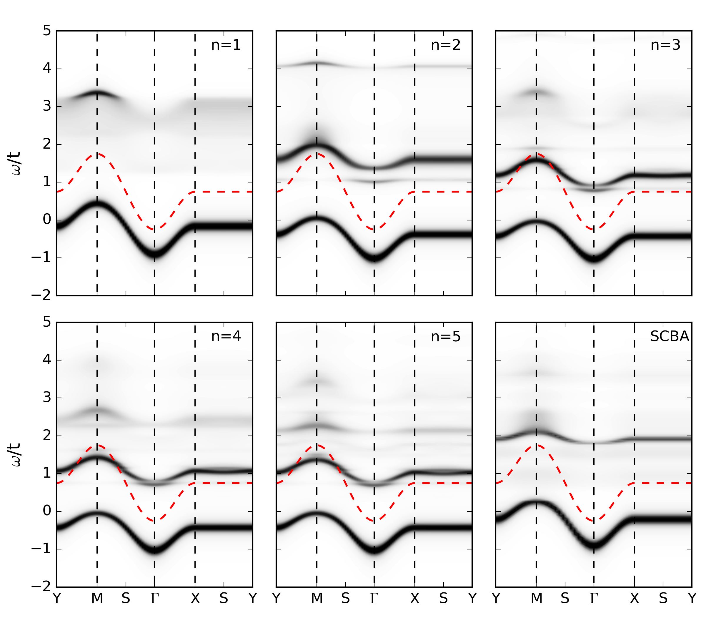
Figure 2: (Color online) Momentum dependence of the spectral function for the variational calculation with a maximum of $n=1$ to $n=5$ orbitons. The 6^th panel shows the corresponding SCBA results. Parameters: $t=1$, $J=0.5$. The dashed red line indicates the free electron dispersion. The spectral function is plotted on a nonlinear $\tanh$-scale to emphasize the low-amplitude incoherent part of the spectrum. The high-symmetry points are: $\Gamma=(0,0)$, $X=(\pi,0)$, $Y=(0,\pi)$, $S=(\pi/2,\pi/2)$, and $M=(\pi,\pi)$.

Fig. 2 shows $A(\mathbf{k},\omega)$ along high symmetry cuts in the Brillouin zone for $n=1$ to $n=5$; the SCBA results are shown in the sixth panel. Note that we cannot show meaningful VCA results for this large $J/t$ value, for reasons explained above. The spectrum consists of a low-energy QP band which has most of the weight, and a broad but low-weight continuum at higher energies. Focusing first on the QP band, we see that with increasing $n$ it moves to lower energies and its bandwidth decreases. This is standard polaronic behavior: a bigger cloud results in a more stable but also heavier polaron. However, we also see that the QP band is already converged for $n\approx 2$, in other words the QP binds very few orbitons in its cloud.

This is expected because for this relatively large $J$, orbiton excitations are expensive. Moreover, the variational approach properly implements the constraint of allowing only up to one orbiton per site. Thus, a cloud with many orbitons would be spread out over many sites. However, the electron can only interact with orbitons on its NN sites, so orbitons that are far from it cost (orbital) exchange energy but do not contribute to a lowering of total energy through carrier-orbiton interactions. As such, their presence is energetically unfavorable.

Another way to think about it is in terms of an “effective coupling”. For lattice polarons, this is defined as $\lambda\sim g^{2}/(\Omega D)$, where $g$ is the (suitably averaged) electron-phonon coupling strength, $\Omega$ is the optical phonon energy and $D$ is the free-electron bandwidth. For small $\lambda$ the polaron cloud has very few phonons and the QP properties are hardly changed compared to those of the free carrier. For large $\lambda$, on the other hand, a so-called “small polaron” forms. It has a large boson cloud, with many phonons, and consequently is a heavy QP.

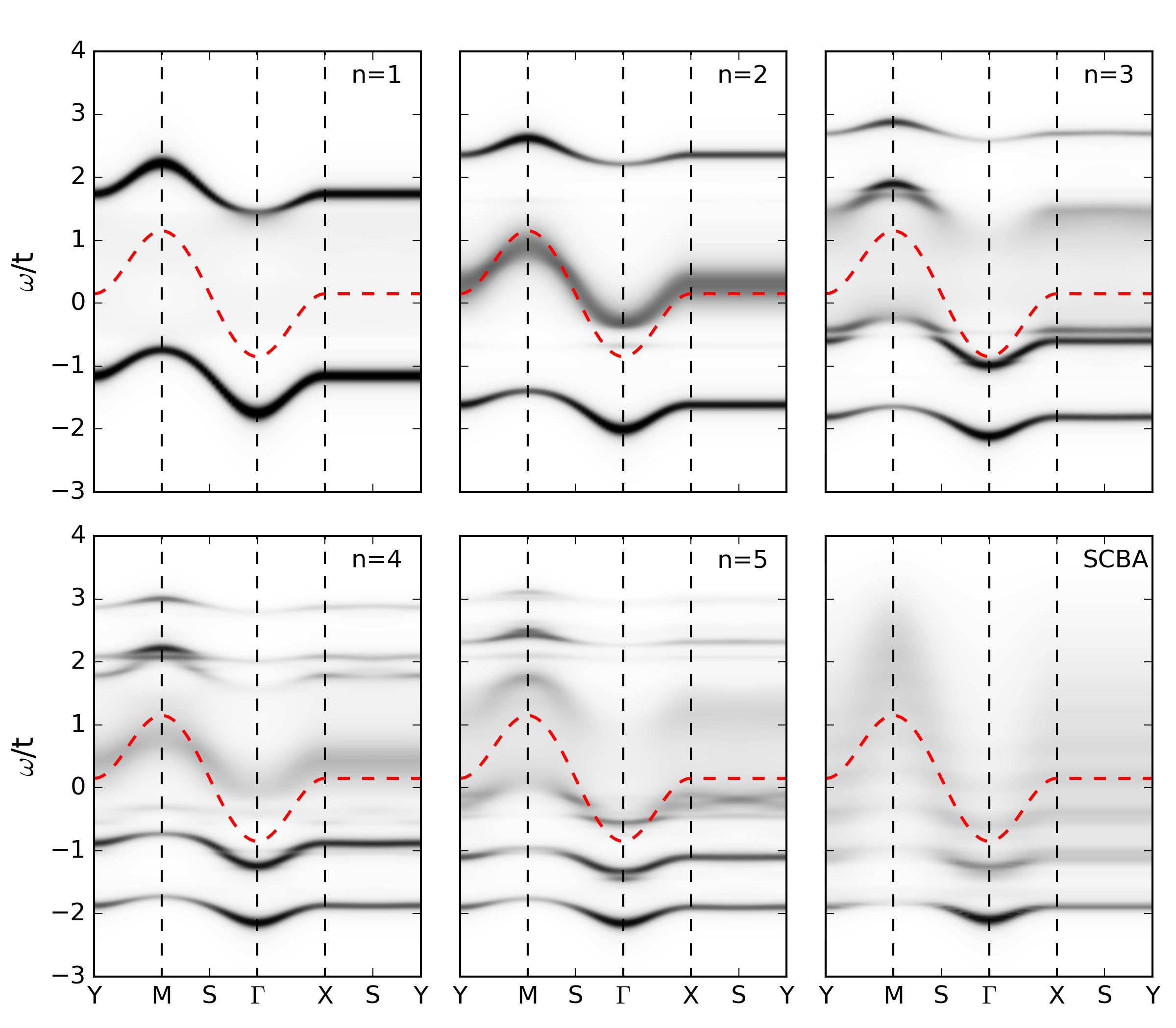
Figure 3: (Color online) Same as in Fig. 2 for $J/t=0.1$. The variational result for $n=6$ is shown in Fig. 6. The high-symmetry points are as in Fig. 2.

For our problem, $g\sim t,D\sim t,\Omega\sim J$; as a result a large $J/t$ implies a small $\lambda$ and vice versa. The results of Fig. 2 are, therefore, consistent with this polaron paradigm of having a small cloud and weakly renormalized QP at small $\lambda$. Moreover, we also see fairly good agreement with SCBA, which is also known to be true for small $\lambda$ Holstein lattice polarons Berciu (2006); Goodvin et al. (2006). This is easy to understand: for a cloud consisting of very few bosons, the probability that the carrier absorbs the last emitted boson (which is the only process allowed in SCBA) as opposed to any other boson, is of order 1. It is only for clouds with many bosons that this probability becomes very small. In this latter case, SCBA is expected to become very inaccurate (as, indeed, is the case for large $\lambda$ Holstein polarons Berciu (2006); Goodvin et al. (2006)) unless there is some other physical reason to strongly favor the absorption of the last emitted boson.

Regarding the higher energy continuum, we see that it keeps on changing up to higher $n$ values, although it converges for $n\approx 5$ (this is why we do not show here the $n=6$ result). This is also expected, because configurations with many orbitons are energetically expensive and contribute primarily to the higher-energy excited states. To properly describe these high-energy states, therefore, one needs to consider bigger variational spaces. The agreement between the variational approach and SCBA is much poorer for this higher energy continuum; we expect the latter to be less accurate here for reasons discussed in the previous paragraph.

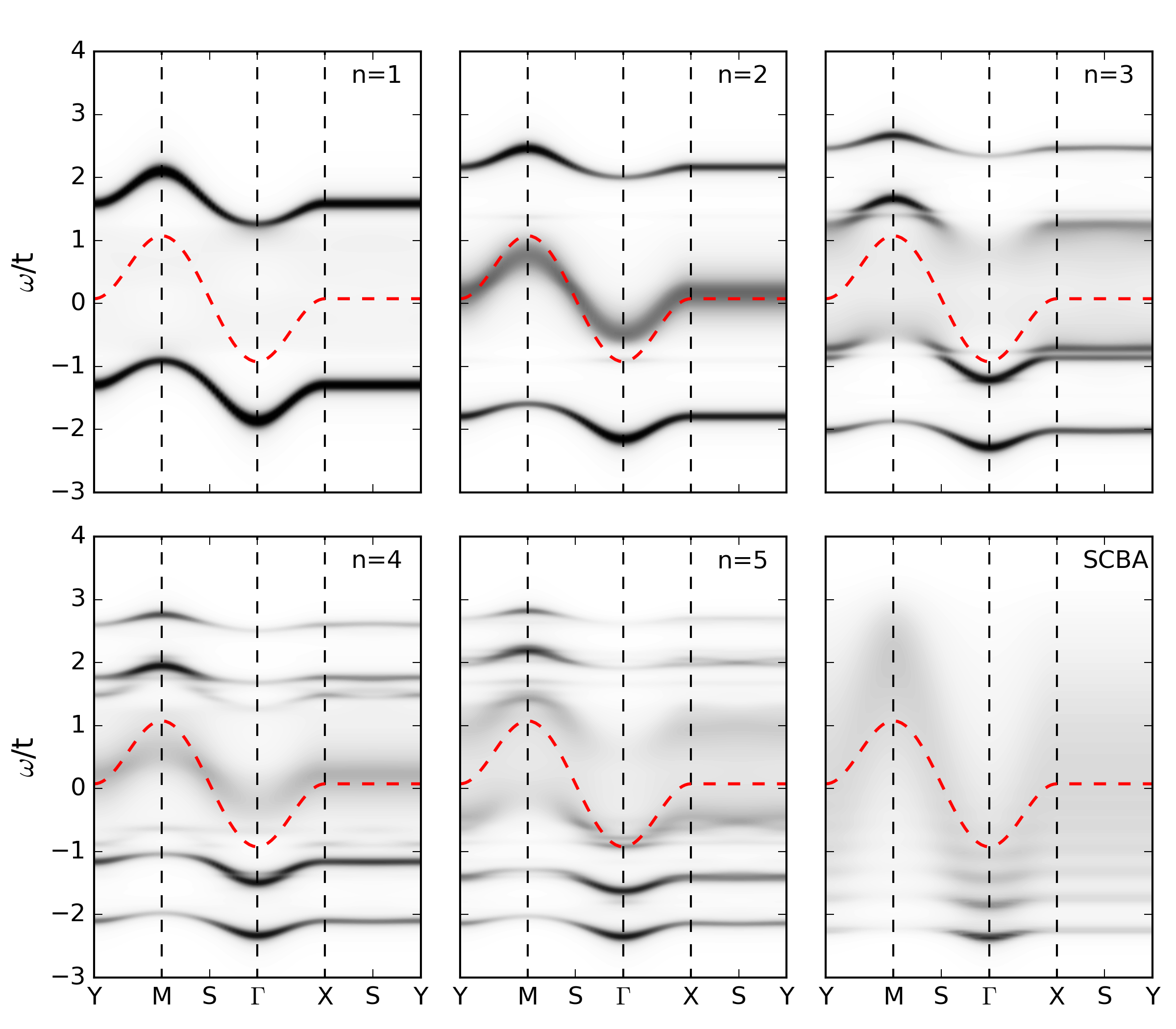
Figure 4: (Color online) Same as in Fig. 2 for $J/t=0.05$. The variational result for $n=6$ is shown in Fig. 6. The high-symmetry points are as in Fig. 2.

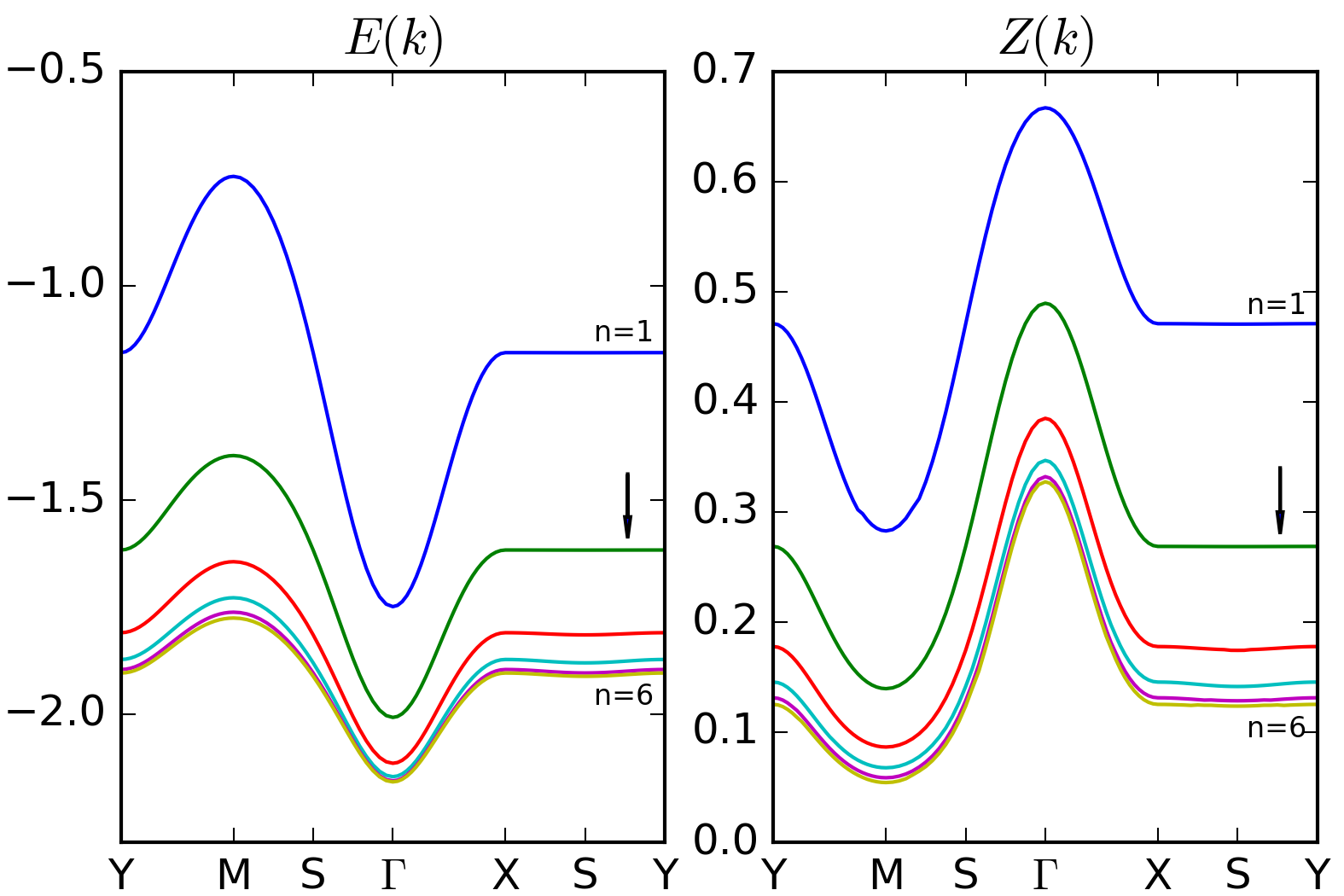
Figure 5: (Color online) Ground state energy $E(\mathbf{k})$ and spectral weight $Z(\mathbf{k})$ calculated numerically for $J=0.1$ (see Fig. 3) and a maximum of $n=1$ to $n=6$ orbitons from top to bottom as indicated by arrows. The high-symmetry points are as in Fig. 2.

We have verified that increasing $J/t$ more, i.e., moving toward even smaller effective couplings, further confirms all the inferences we have made so far. Clearly, the more interesting question is what happens in the opposite limit, when the effective coupling increases. This is shown in Figs. 3 and 4 for $J/t=0.1$ and 0.05, respectively. As expected, as we move towards stronger effective coupling, the QP band reaches convergence more slowly (at $n\approx 5$ in these cases), moves to even lower energies and becomes narrower. For a more direct verification of this see Fig. 5 showing the evolution of QP energy $E(\mathbf{k})$ and spectral weight $Z(\mathbf{k})$ for increasing number of orbitons at $J=0.1$. One can clearly see the monotonic convergence of the ground state results, as should indeed be the case for the variational method. Both of the curves are practically indistinguishable from one another for the cases $n=5$ and $n=6$, indicating that the result is practically converged for $n\approx 5$.

The higher energy continuum is also more structured, but it is probably not yet fully converged. On the low-energy side, it exhibits “copies” of the QP band. The agreement with SCBA for the QP band is quite good for $J/t=0.1$, but for $J/t=0.05$ SCBA predicts a much heavier polaron than the variational approximation (see also Sec. IV.2 below). This is likely due to the fact that SCBA does not enforce the constraint of allowing only up to one orbiton per site. As a result, at strong couplings it is likely to overestimate the number of orbitons in the QP cloud, and therefore predict a heavier QP.

IV.2 Comparison with VCA

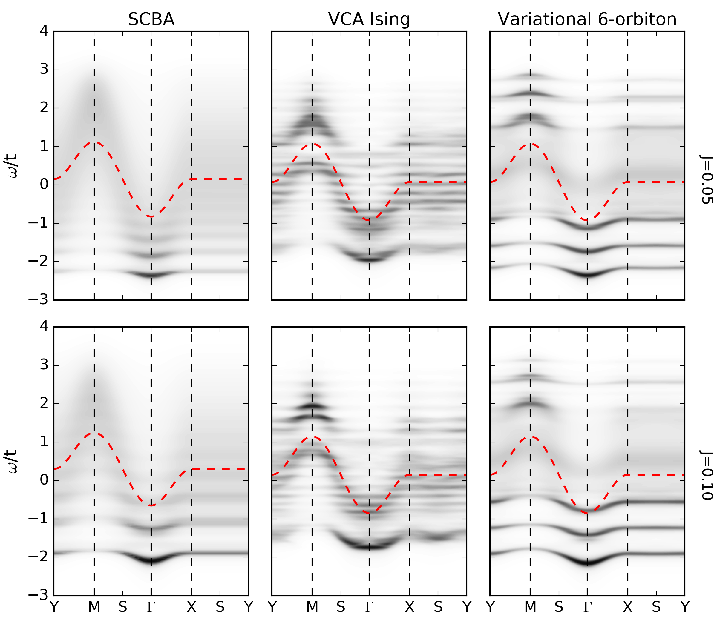
Figure 6: (Color online) Comparison of the spectral weights predicted by SCBA (left), VCA (center) and the variational approach with $n=6$, for $J/t=0.05$ (top panels) and 0.1 (bottom panels). The high-symmetry points are as in Fig. 2.

Figure 6 presents the comparison of the spectral function for $J/t=0.05$ and 0.1, for SCBA, VCA and the variational approach with $n=6$ orbitons. On the first glance, the QP band in the VCA solution looks more similar to the variational result, but as shown below the SCBA gives also quite satisfactory results for the QPs. Although all the solutions exhibit a similar shape, with a lot of spectral weight around the minimum at the $\Gamma=(0,0)$ point and a substantial drop in weight with additional flattening of the spectrum around the $M=(\pi,\pi)$ point, those features are much more pronounced in the SCBA than in the other two methods.

Above the QP band, both SCBA and the variational approach show the emergence of a ladder structure of excited states dissolving quickly into a broad continuum. Such a “shake-off” band also emerges below the continuum for VCA for $J/t=0.05$, although its weight is rather small. Thus, it seems reasonable to expect that such a feature does emerge in the strong coupling limit, although the variational method and SCBA may overestimate it.

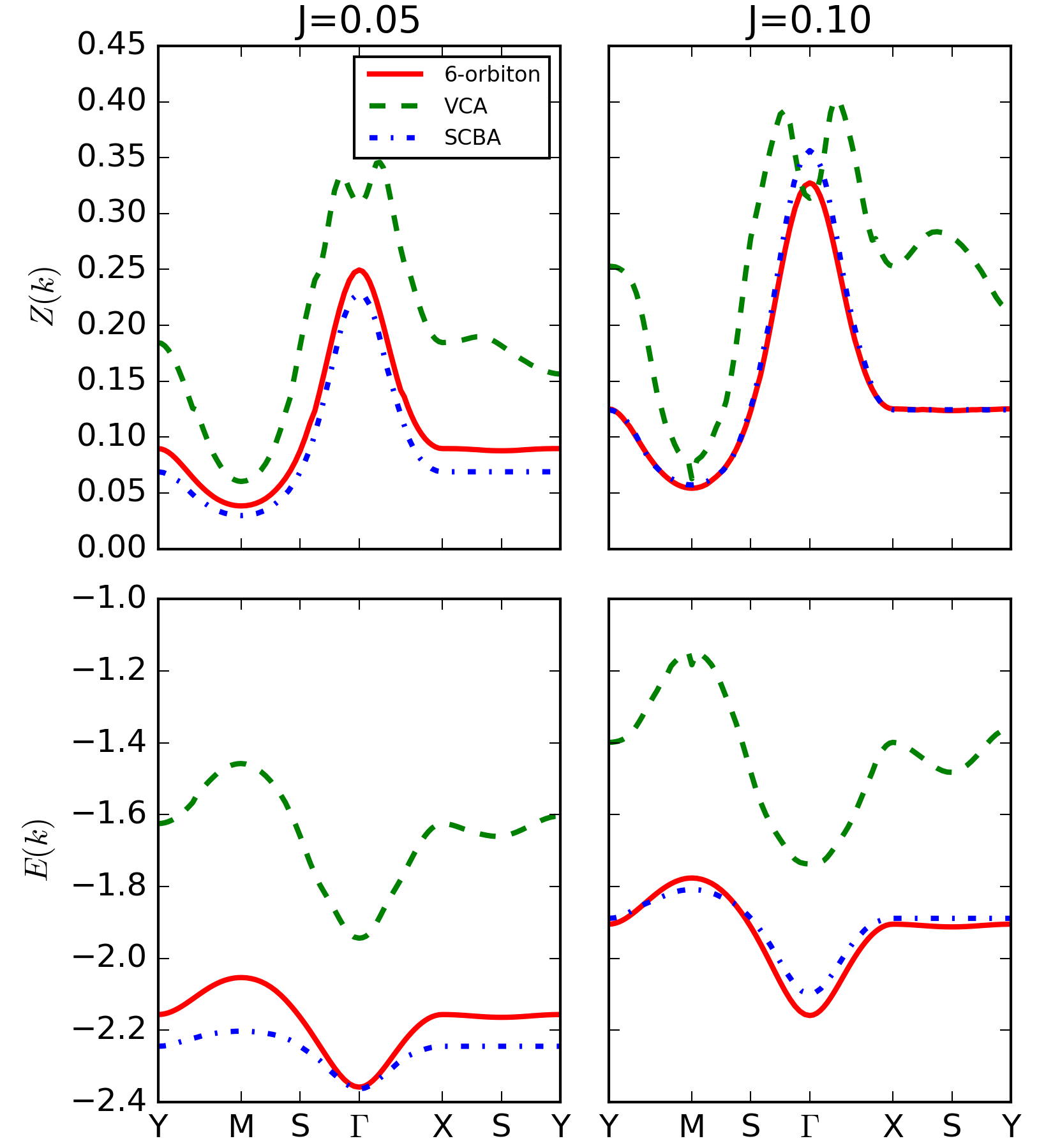
Figure 7: (Color online) Spectral weight $Z(\mathbf{k})$ (top) and ground-state energy $E(\mathbf{k})$ (bottom) for $J=0.05$ (left) and 0.10 (right) as obtained in the $n=6$ orbiton variational approach (6-orbiton), in VCA and in SCBA. The high-symmetry points are as in Fig. 2.

At even higher energies, SCBA predicts a very featureless continuum, unlike VCA and the present variational method, which show a more structured one. However, since neither SCBA nor the variational method aim to be highly accurate at such high energies, such comparisons are of limited use. It should also be noted that the apparent dense peak structure obfuscating the VCA results is not physical but just a finite-size effect which is the usual byproduct of this method.

Returning to the low-energy polaron, we show its QP spectral weights $Z(\mathbf{k})$ and ground state energies $E(\mathbf{k})$ in Fig. 7, obtained by least squares fitting of a Lorentzian curve to the first peak of the spectrum. As can be seen, while SCBA and the variational result are in good agreement as to the spectral weight in both of the presented cases, SCBA always predicts a heavier QP, especially for the smaller value of $J$, where it clearly overestimates the binding energy due to not including the particle constraints, as already discussed. On the other hand, one can see that the VCA results are in disagreement with both other results. This can be attributed partly to those calculations being based on a different model, and so can be affected by a ground state energy shift, and partly due to the systematic error of the method as demonstrated by the dense peak structure, which affects the quality of the peak fit. In any case, the VCA results are in agreement with other results only qualitatively, although they are usually more similar to the variational results.

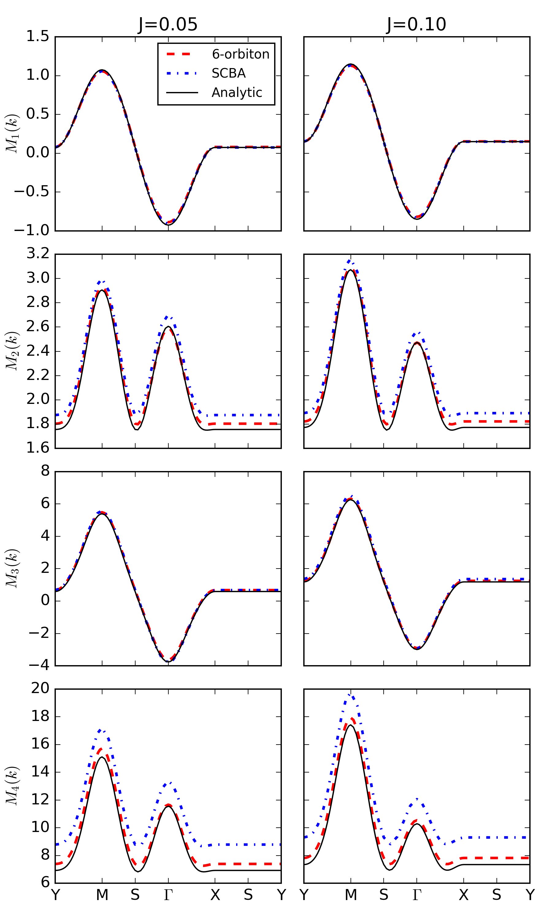
Figure 8: (Color online) First four spectral moments for the calculations performed in the one-orbiton and two-orbiton variational approximation, and SCBA as compared to the analytical solution. The high-symmetry points as in Fig. 2.

As a final way to compare SCBA and the variational approach in the strong coupling limit, Fig. 8 shows the predicted first four spectral moments compared to their analytical expressions. While the agreement is reasonable for both methods up to $M_{3}(\mathbf{k})$, the variational approach is clearly more accurate. Note however, that while agreement with sum rules is obviously desirable, nevertheless one has to be careful when assessing how meaningful such an agreement really is Goodvin et al. (2006).

IV.3 Significance of inter-orbital hopping

After discussing the similarities and differences between the SCBA and the variational approach, let us briefly focus on the relative importance of the $t$ and $J$ energy scales for the QP propagation. In the strong coupling limit, Fig. 7 shows that the QP bandwidth changes with $r=J/t$, but this dependence is rather weak for VCA and the variational approach. The bandwidth is reduced from the free value expected for unhindered inter-orbital hopping, but it is clearly not proportional to $J$.

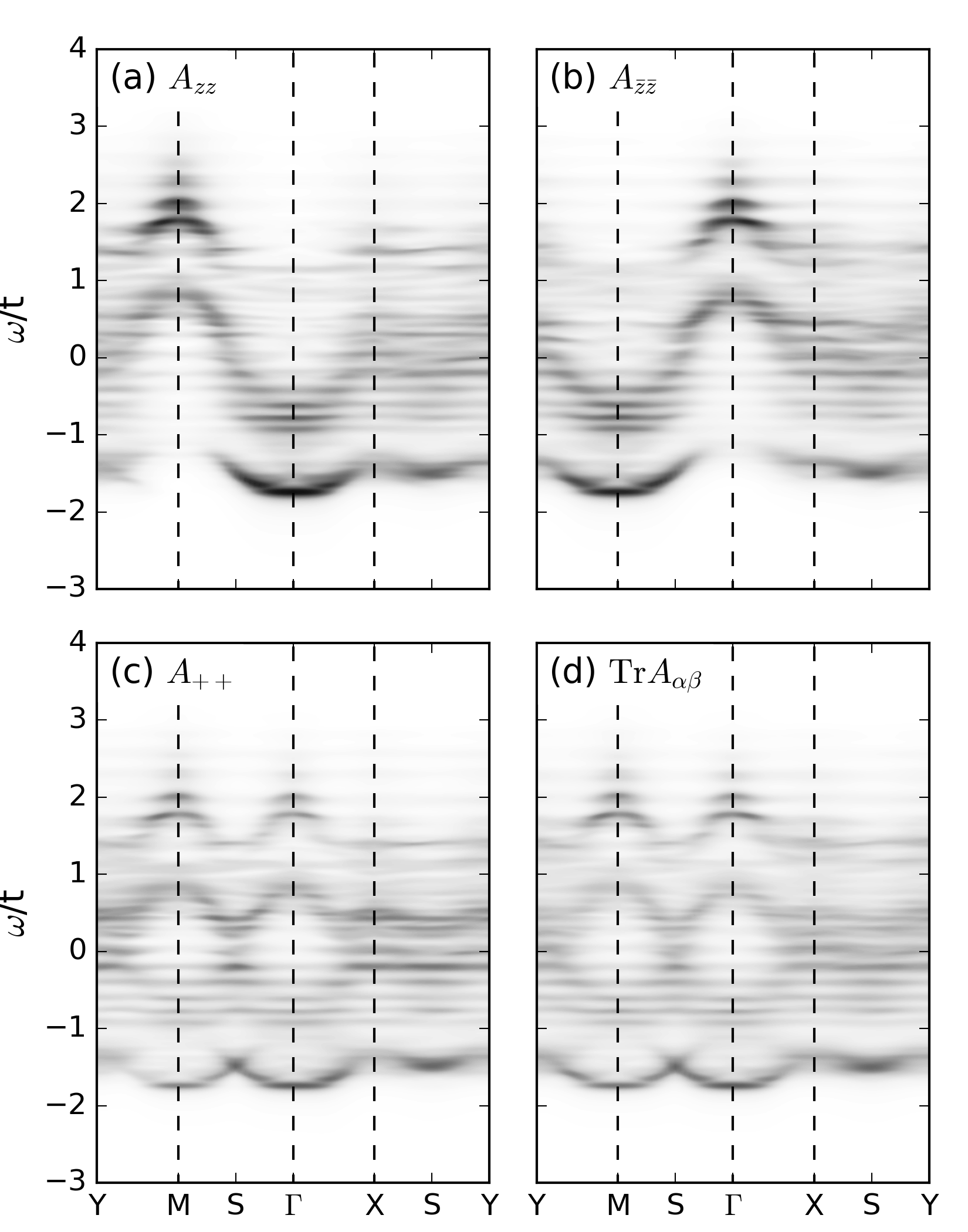
Figure 9: VCA-spectra for AO state at $U=10t$ (corresponding to $J=0.10$) and: (a) the $\lvert z\rangle$ orbital, (b) the $\lvert\bar{z}\rangle$ orbital, (c) the orbital $\lvert+\rangle$, as well as (d) the trace over the orbital basis (basis invariant), i.e., the normalized sum of (a) and (b). The high-symmetry points as in Fig. 2.

We can further substantiate the importance of inter-orbital hopping by looking at orbitally resolved spectra. To do so, here we show the hole spectra projected onto the original $\lvert z\rangle$ and $\lvert\bar{z}\rangle$ orbitals. These are given by

$$A_{\alpha\alpha}(\vec{k},\omega)=$$ (40)

$$-\frac{1}{\pi}\lim_{\delta\to 0}\Im\left[\langle 0|c^{\dagger}_{\vec{k}\alpha}\frac{1}{\omega-(\mathcal{H}_{t}+\mathcal{H}_{U}-E_{0})+i\delta}c_{\vec{k}\alpha}|0\rangle\right],$$

for $\alpha=z,\bar{z}$ referring to the $3z^{2}-r^{2}$ and $x^{2}-y^{2}$ orbitals (2). $\mathcal{H}_{t}+\mathcal{H}_{U}$ is the ‘Hubbard-like’ Hamiltonian comprised of Eqs. (6) and (3), whose half-filled ground state is denoted by $|0\rangle$ and has energy $E_{0}$. Spectra for $z$ and $\bar{z}$ are shown in Figs. 9(a) and 9(b), respectively.

The first notable feature is that the dispersion does not reflect the doubled unit cell of the AO ground state, as might a priori be expected. This doubling of the unit cell does manifest itself in the spectrum calculated for the orbital $\lvert\alpha\rangle=\lvert+\rangle$, see Fig. 9(c), and in the trace shown in Fig. 9(d). The second relevant aspect is that the dispersion is “opposite” for the $\lvert z\rangle$ and $\lvert\bar{z}\rangle$ orbitals, i.e., the minimum is either at the $\Gamma$ point (for $\lvert z\rangle$) or at the $M$ point (for $\lvert\bar{z}\rangle$).

Such an orbital-specific lack of any signature of the unit-cell size is not expected in a propagation mechanism driven by three-site terms or orbital flips, and doubling of the unit cell is in fact observed in the $t_{2g}$ or SU(2) symmetric $t$-$J$ models. However, this feature arises naturally for a dispersion supported mainly by inter-orbital NN hopping. The AO ordered ground state consist of alternating $\lvert+\rangle$ and $\lvert-\rangle$ orbitals occupying sublattices $a$ and $b$ respectively. The interorbital hopping $t_{+-}=t/4$ allows a $\lvert+\rangle$ electron on sublattice $a$ to move to the $\lvert-\rangle$ orbital of a previously empty NN site on sublattice $b$ – the hole has thus moved between NN sites without disturbing the AO background. The $\lvert z\rangle$ orbital has positive overlap $+\tfrac{1}{\sqrt{2}}$ with both $\lvert\pm\rangle$ orbitals and consequently a minimum develops at $\Gamma$ like for a free particle, see Fig. 9(a). The $\lvert\bar{z}\rangle$ orbital, on the other hand, has an overlap $\pm\tfrac{1}{\sqrt{2}}$ alternating from site to site. It translates into the momentum shift moving the minimum to $M$, as observed in Fig. 9(b).

We have thus identified interorbital hopping as the main driving force of hole propagation in the $e_{g}$ model. While the bandwidth is reduced from its free value through interaction with the AO background, the SCBA overestimates this effect. This may in turn assign too strong a role to orbital fluctuations and consequently obscure the origin of the QP propagation. Finally, we note that an orbital-selective ARPES study might fail to see the doubling of the unit cell of an orbitally ordered state, depending on the wave function of the ordered orbital.

V Conclusions

By analogy with work done for other polaron models, here we constructed a method to calculate the Green’s function for an orbiton-polaron in a variational space including configurations with up to six orbitons. We then compared these results with two different and well established methods, SCBA and VCA. We found that our variational Green’s function converges fast, especially for the low-energy QP, and that this important feature agrees well with the corresponding feature obtained in VCA in the strong effective coupling limit. In contrast, the quasiparticle predicted by SCBA has a noticeably smaller bandwidth, although general quantitative trends of the spectra are similar for all three methods.

The higher accuracy of the variational approach can be understood by noting that its equations of motions allow orbitons to be absorbed in any order and it consequently includes crossed diagrams, which are neglected by the SCBA. Moreover, it also implements the local constraints ignored by SCBA. In fact, at first sight it is perhaps surprising that the agreement with SCBA remains as good as it is in the strong effective coupling limit. This is in contrast to what happens for lattice polarons but in agreement with what is observed for spin polarons. The common link with the latter is that like magnons, orbitons are also restricted to at most one per site. As a result, the cloud is spread over a larger area and the carrier is more likely to absorb one of the last emitted orbitons, since they are close to its location (note that at energies characteristic for the polaron band, which lie well below the free-particle band, the free carrier cannot propagate). Thus, even though there is no analogue of the total spin conservation, which leads to the vanishing of many crossed diagrams and thus improves the validity of SCBA for spin models, uncrossed diagrams still have higher probabilities than crossed ones in the present problem. By contrast, in the small polaron limit of a lattice polaron, the number $n$ of phonons on the same site can be quite large. Because they are indistinguishable, the carrier is equally likely to absorb them in any of $n!$ possible orders, and SCBA, which only allows them to be absorbed in the order inverse to that of their creation, underestimates the contribution of such processes by $1/n!$.

An interesting follow-up question is whether SCBA is still expected to be qualitatively accurate (even though quantitatively less accurate than the variational method) for the combined spin-orbiton polarons Wohlfeld et al. (2009), given that it performs reasonably well for either species of bosons. We expect this to not be the case, because there is no reason why diagrams with crossed magnon and orbiton lines should be small compared to the non-crossed ones included in SCBA: magnons and orbitons can be located on the same site and there is no conservation law restricting the order in which they can be absorbed.

Moreover, SCBA does not lend itself easily to schemes with multiple bosonic flavors, which would be the case for the spin-orbital problem, while the variational method proposed here has already proved highly accurate for spin-polaron problems (as well as lattice polaron problems), and can be easily extended to such multi-boson models. It is thus a promising candidate for investigating carrier propagation in the full 3D $A$-AF/$C$-AO order in KCuF₃ which needs to include both orbiton and spin degrees of freedom, similar to LaMnO₃ Bała et al. (2001). Such studies are under way at present.

Appendix A Details of the two-orbiton solution

The two-orbiton solution is derived similarly to the one-orbiton case, but with the orbiton number cutoff set at two. This has no effect on Eqs. (15) to (23), which therefore remain unchanged. The difference appears first in the equations of motion for the $F_{1}$ propagators, which now also acquire two orbitons propagators on their right hand side in addition to the terms already listed in Eqs. (24) and (25) indicated here by “$\ldots$”, respectively:

$$F_{1}^{(2)}(\mathbf{k},\omega,\delta) =\ldots-\frac{t}{4}\sum_{\gamma\epsilon}\left[2F_{2}(\mathbf{k},\omega,\epsilon,\gamma)-\sqrt{3}\bar{F}_{2}(\mathbf{k},\omega,\epsilon,\gamma)e^{i\pi_{y}\cdot\gamma}\right]G_{1}(i+\epsilon,i+\delta,\omega),$$ (41)

$$\bar{F}_{1}^{(2)}(\mathbf{k},\omega,\delta) =\ldots-\frac{t}{4}\sum_{\gamma\epsilon}\left[2\bar{F}_{2}(\mathbf{k},\omega,\epsilon,\gamma)-\sqrt{3}F_{2}(\mathbf{k},\omega,\epsilon,\gamma)e^{i\pi_{y}\cdot\gamma}\right]G_{1}(i+\epsilon,i+\delta,\omega).$$ (42)

The generalized Green’s functions for states with two orbitons are defined as:

$$F_{2}(\mathbf{k},\omega,\epsilon,\gamma) =\langle\mathbf{k}\rvert\mathcal{G}(\omega)\frac{1}{\sqrt{N}}\sum_{i}e^{i\mathbf{k}\cdot\mathbf{R}_{i}}f_{i+\epsilon+\gamma}^{{\dagger}}a_{i+\epsilon}^{{\dagger}}a_{i}^{{\dagger}}\lvert 0\rangle,$$ (43)

$$\bar{F}_{2}(\mathbf{k},\omega,\epsilon,\gamma) =\langle\mathbf{k}\rvert\mathcal{G}(\omega)\frac{1}{\sqrt{N}}\sum_{i}e^{i(\mathbf{k+Q})\cdot\mathbf{R}_{i}}f_{i+\epsilon+\gamma}^{{\dagger}}a_{i+\epsilon}^{{\dagger}}a_{i}^{{\dagger}}\lvert 0\rangle.$$ (44)

The equations of motion for these propagators are calculated using again Dyson’s equation. To simplify the analytical solution, we impose the additional constraint that only configurations with the two orbitons located on adjacent sites are kept in the variational space. As shown in Sec. IV.1, the numerical solution shows that this is a good approximation for the low-energy quasiparticle. Because of this and because the orbiton number cutoff is set at two, the equations of motion for $F_{2}$ and $\bar{F}_{2}$ are linked only to one-orbiton Green’s functions:

$$F_{2}(\mathbf{k},\omega,\epsilon,\gamma)=-\frac{t}{4}\sum_{\beta} \left[(2F_{1}(\mathbf{k},\omega,\epsilon)-\sqrt{3}\bar{F}_{1}(\mathbf{k},\omega,\epsilon)e^{i\pi_{y}\cdot\beta})G_{2}(i+\epsilon+\beta,i+\epsilon+\gamma)\right.$$

$$\left.+(2F_{1}(\mathbf{k},\omega,-\epsilon)-\sqrt{3}\bar{F}_{1}(\mathbf{k},\omega,-\epsilon)e^{i\pi_{y}\cdot\beta})e^{-i\mathbf{k}\cdot\epsilon}G_{2}(i+\beta,i+\epsilon+\gamma)\right],$$ (45)

$$\bar{F}_{2}(\mathbf{k},\omega,\epsilon,\gamma)=-\frac{t}{4}\sum_{\beta} \left[(2\bar{F}_{1}(\mathbf{k},\omega,\epsilon)-\sqrt{3}F_{1}(\mathbf{k},\omega,\epsilon)e^{i\pi_{y}\cdot\beta})G_{2}(i+\epsilon+\beta,i+\epsilon+\gamma)\right.$$

$$\left.-(2\bar{F}_{1}(\mathbf{k},\omega,-\epsilon)-\sqrt{3}F_{1}(\mathbf{k},\omega,-\epsilon)e^{i\pi_{y}\cdot\beta})e^{-i\mathbf{k}\cdot\epsilon}G_{2}(i+\beta,i+\epsilon+\gamma)\right],$$ (46)

where $G_{2}$ functions are real space, non-interacting Green’s functions with spatial constraints imposed by the presence of two orbitons in the system. They are analogous to the $G_{1}$ functions defined in equations (18) to (21), only this time we need to subtract from the Hamiltonian the terms corresponding to both sites occupied by the orbitons, namely $\{i,i+\epsilon\}$. The equation defining these Green’s functions is virtually identical to Eq. (21), only the range of summation changes. In fact, the general expression for a constrained Green’s function describing a real-space propagation from site $m$ to site $n$ in a 2D system with a string of orbitons of length $l$ can be written as:

$$G_{l}(n,m,\omega)=G_{0}(n,m,\omega-rJ^{\prime})+\sum_{\langle p,\tilde{p}\rangle}G_{l}(n,p,\omega)\\ \times\left[\frac{t}{4}G_{0}(\tilde{p},m,\omega-rJ^{\prime})-2J^{\prime}G_{0}(p,m,\omega-rJ^{\prime})\right],$$ (47)

where the index $\tilde{p}$ goes over all the sites occupied by an orbiton and $p$ goes over all the unoccupied sites adjacent to a given $\tilde{p}$, with the summation going over all such pairs of sites; $r=4(l+2)$, so in our case $r=16$.

Taken together, these equations define a (bigger) linear system of inhomogeneous equations, which are then solved to find the solution in this larger variational space. A generalization to more orbitons follows along similar lines. In the case of $n=6$ orbitons, the equations of motions for propagators $F_{n}$ with $n\leq 6$ are generated and solved numerically.

References

- Zaanen and Oleś (1993) J. Zaanen and A. M. Oleś, Phys. Rev. B 48, 7197 (1993).
- Wohlfeld et al. (2009) K. Wohlfeld, A. M. Oleś, and P. Horsch, Phys. Rev. B 79, 224433 (2009).
- Lee et al. (2006) P. A. Lee, N. Nagaosa, and X.-G. Wen, Rev. Mod. Phys. 78, 17 (2006).
- Tohyama and Maekawa (1994) T. Tohyama and S. Maekawa, Phys. Rev. B 49, 3596 (1994).
- Bała et al. (1995) J. Bała, A. M. Oleś, and J. Zaanen, Phys. Rev. B 52, 4597 (1995).
- Martínez and Horsch (1991) G. Martínez and P. Horsch, Phys. Rev. B 44, 317 (1991).
- Trugman (1988) S. A. Trugman, Phys. Rev. B 37, 1597 (1988).
- Kugel and Khomskii (1982) K. I. Kugel and D. I. Khomskii, Sov. Phys. Usp. 25, 231 (1982).
- Feiner et al. (1997) L. F. Feiner, A. M. Oleś, and J. Zaanen, Phys. Rev. Lett. 78, 2799 (1997).
- Feiner et al. (1998) L. F. Feiner, A. M. Oleś, and J. Zaanen, J. Phys.: Condens. Matter 10, L555 (1998).
- Feiner and Oleś (1999) L. F. Feiner and A. M. Oleś, Phys. Rev. B 59, 3295 (1999).
- Khaliullin and Maekawa (2000) G. Khaliullin and S. Maekawa, Phys. Rev. Lett. 85, 3950 (2000).
- Khaliullin et al. (2001) G. Khaliullin, P. Horsch, and A. M. Oleś, Phys. Rev. Lett. 86, 3879 (2001).
- Khaliullin et al. (2004) G. Khaliullin, P. Horsch, and A. M. Oleś, Phys. Rev. B 70, 195103 (2004).
- Oleś et al. (2005) A. M. Oleś, G. Khaliullin, P. Horsch, and L. F. Feiner, Phys. Rev. B 72, 214431 (2005).
- Khaliullin (2005) G. Khaliullin, Prog. Theor. Phys. Suppl. 160, 155 (2005).
- Reitsma et al. (2005) A. J. W. Reitsma, L. F. Feiner, and A. M. Oleś, New J. Phys. 5, 121 (2005).
- Cuoco et al. (2006) M. Cuoco, F. Forte, and C. Noce, Phys. Rev. B 74, 195124 (2006).
- Chaloupka and Khaliullin (2008) J. Chaloupka and G. Khaliullin, Phys. Rev. Lett. 100, 016404 (2008).
- Krüger et al. (2009) F. Krüger, S. Kumar, J. Zaanen, and J. van den Brink, Phys. Rev. B 79, 054504 (2009).
- Corboz et al. (2012) P. Corboz, M. Lajkó, A. M. Läuchli, K. Penc, and F. Mila, Phys. Rev. X 2, 041013 (2012).
- Brzezicki et al. (2012) W. Brzezicki, J. Dziarmaga, and A. M. Oleś, Phys. Rev. Lett. 109, 237201 (2012).
- Brzezicki et al. (2013) W. Brzezicki, J. Dziarmaga, and A. M. Oleś, Phys. Rev. B 87, 064407 (2013).
- Brzezicki and Oleś (2011) W. Brzezicki and A. M. Oleś, Phys. Rev. B 83, 214408 (2011).
- Czarnik and Dziarmaga (2015) P. Czarnik and J. Dziarmaga, Phys. Rev. B 91, 045101 (2015).
- Wohlfeld et al. (2011) K. Wohlfeld, M. Daghofer, S. Nishimoto, G. Khaliullin, and J. van den Brink, Phys. Rev. Lett. 107, 147201 (2011).
- Marra et al. (2012) P. Marra, K. Wohlfeld, and J. van den Brink, Phys. Rev. Lett. 109, 117401 (2012).
- Bisogni et al. (2015) V. Bisogni, K. Wohlfeld, S. Nishimoto, C. Monney, J. Trinckauf, K. Zhou, R. Kraus, K. Koepernik, C. Sekar, V. Strocov, B. Büchner, T. Schmitt, J. van den Brink, and J. Geck, Phys. Rev. Lett. 114, 096402 (2015).
- Wohlfeld et al. (2013) K. Wohlfeld, S. Nishimoto, M. W. Haverkort, and J. van den Brink, Phys. Rev. B 88, 195138 (2013).
- Chen et al. (2015) C.-C. Chen, M. van Veenendaal, T. P. Devereaux, and K. Wohlfeld, Phys. Rev. B 91, 165102 (2015).
- Brzezicki et al. (2014a) W. Brzezicki, J. Dziarmaga, and A. M. Oleś, Phys. Rev. Lett. 112, 117204 (2014a).
- Smerald and Mila (2014) A. Smerald and F. Mila, Phys. Rev. B 90, 094422 (2014).
- Avella et al. (2015) A. Avella, A. M. Oleś, and P. Horsch, Phys. Rev. Lett. 115, 206403 (2015).
- Avella et al. (2013) A. Avella, P. Horsch, and A. M. Oleś, Phys. Rev. B 87, 045132 (2013).
- Horsch and Oleś (2011) P. Horsch and A. M. Oleś, Phys. Rev. B 84, 064429 (2011).
- Brzezicki et al. (2015a) W. Brzezicki, A. M. Oleś, and M. Cuoco, Phys. Rev. X 5, 011037 (2015a).
- Brzezicki et al. (2016) W. Brzezicki, M. Cuoco, and A. M. Oleś, J. Sup. Novel Magn. 29, in press (2016).
- Oleś (2012) A. M. Oleś, J. Phys.: Condens. Matter 24, 313201 (2012).
- Oleś (2015) A. M. Oleś, Acta Phys. Polon. A 127, 163 (2015).
- Oleś et al. (2006) A. M. Oleś, P. Horsch, L. F. Feiner, and G. Khaliullin, Phys. Rev. Lett. 96, 147205 (2006).
- You et al. (2015a) W.-L. You, A. M. Oleś, and P. Horsch, New J. Phys. 17, 083009 (2015a).
- You et al. (2012) W.-L. You, A. M. Oleś, and P. Horsch, Phys. Rev. B 86, 094412 (2012).
- You et al. (2015b) W.-L. You, P. Horsch, and A. M. Oleś, Phys. Rev. B 92, 054423 (2015b).
- van Rynbach et al. (2010) A. van Rynbach, S. Todo, and S. Trebst, Phys. Rev. Lett. 105, 146402 (2010).
- van den Brink et al. (1999) J. van den Brink, P. Horsch, F. Mack, and A. M. Oleś, Phys. Rev. B 59, 6795 (1999).
- Tanaka et al. (2005) T. Tanaka, M. Matsumoto, and S. Ishihara, Phys. Rev. Lett. 95, 267204 (2005).
- Tanaka and Ishihara (2009) T. Tanaka and S. Ishihara, Phys. Rev. B 79, 035109 (2009).
- Feiner and Oleś (2005) L. F. Feiner and A. M. Oleś, Phys. Rev. B 71, 144422 (2005).
- Khaliullin and Kilian (2000) G. Khaliullin and R. Kilian, Phys. Rev. B 61, 3494 (2000).
- Oleś and Feiner (2002) A. M. Oleś and L. F. Feiner, Phys. Rev. B 65, 052414 (2002).
- Daghofer et al. (2008) M. Daghofer, K. Wohlfeld, A. M. Oleś, E. Arrigoni, and P. Horsch, Phys. Rev. Lett. 100, 066403 (2008).
- Wohlfeld et al. (2008) K. Wohlfeld, M. Daghofer, A. M. Oleś, and P. Horsch, Phys. Rev. B 78, 214423 (2008).
- Wróbel and Oleś (2010) P. Wróbel and A. M. Oleś, Phys. Rev. Lett. 104, 206401 (2010).
- Brzezicki et al. (2014b) W. Brzezicki, M. Daghofer, and A. M. Oleś, Phys. Rev. B 89, 024417 (2014b).
- Brzezicki et al. (2015b) W. Brzezicki, M. Daghofer, and A. M. Oleś, Acta Phys. Polon. A 127, 263 (2015b).
- Daghofer et al. (2004) M. Daghofer, A. M. Oleś, and W. von der Linden, Phys. Rev. B 70, 184430 (2004).
- van den Brink et al. (2000) J. van den Brink, P. Horsch, and A. M. Oleś, Phys. Rev. Lett. 85, 5174 (2000).
- Paolasini et al. (2002) L. Paolasini, R. Caciuffo, A. Sollier, P. Ghigna, and M. Altarelli, Phys. Rev. Lett. 88, 106403 (2002).
- Lake et al. (2005) B. Lake, D. A. Tennant, C. D. Frost, and S. E. Nagler, Nature Mat. 4, 329 (2005).
- Cincio et al. (2010) L. Cincio, J. Dziarmaga, and A. M. Oleś, Phys. Rev. B 82, 104416 (2010).
- Daghofer et al. (2006) M. Daghofer, A. M. Oleś, D. R. Neuber, and W. von der Linden, Phys. Rev. B 73, 104451 (2006).
- Berciu (2006) M. Berciu, Phys. Rev. Lett. 97, 036402 (2006).
- Berciu (2007) M. Berciu, Phys. Rev. Lett. 98, 209702 (2007).
- Marchand et al. (2010) D. J. J. Marchand, G. De Filippis, V. Cataudella, M. Berciu, N. Nagaosa, N. V. Prokof’ev, A. S. Mishchenko, and P. C. E. Stamp, Phys. Rev. Lett. 105, 266605 (2010).
- Berciu and Fehske (2011) M. Berciu and H. Fehske, Phys. Rev. B 84, 165104 (2011).
- Trousselet et al. (2013) F. Trousselet, M. Berciu, A. M. Oleś, and P. Horsch, Phys. Rev. Lett. 111, 037205 (2013).
- Ebrahimnejad et al. (2014) H. Ebrahimnejad, G. A. Sawatzky, and M. Berciu, Nature Physics 10, 951 (2014).
- (68) H. Ebrahimnejad, G. A. Sawatzky, and M. Berciu, arXiv:1505.04405 (unpublished) .
- Morita and Horiguchi (1971) T. Morita and T. Horiguchi, J. Phys. Soc. Jpn. 30, 957 (1971).
- Morita (1971) T. Morita, J. Math. Phys. 12, 1744 (1971).
- Ramšak and Horsch (1998) A. Ramšak and P. Horsch, Phys. Rev. B 57, 4308 (1998).
- Potthoff et al. (2003) M. Potthoff, M. Aichhorn, and C. Dahnken, Phys. Rev. Lett. 91, 206402 (2003).
- Dahnken et al. (2004) C. Dahnken, M. Aichhorn, W. Hanke, E. Arrigoni, and M. Potthoff, Phys. Rev. B 70, 245110 (2004).
- Nolting (1972) W. Nolting, Z. Phys. B 255, 25 (1972).
- Goodvin et al. (2006) G. L. Goodvin, M. Berciu, and G. A. Sawatzky, Phys. Rev. B 74, 245104 (2006).
- Bała et al. (2001) J. Bała, G. A. Sawatzky, A. M. Oleś, and A. Macridin, Phys. Rev. Lett. 87, 067204 (2001).