Strange resonance poles from $K\pi$ scattering below 1.8 GeV

Abstract

In this work we present a determination of the mass, width, and coupling of the resonances that appear in kaon-pion scattering below 1.8 GeV. These are: the much debated scalar $\kappa$-meson, nowadays known as $K_{0}^{*}(800)$, the scalar $K_{0}^{*}(1430)$, the $K^{*}(892)$ and $K_{1}^{*}(1410)$ vectors, the spin-two $K_{2}^{*}(1430)$ as well as the spin-three $K^{*}_{3}(1780)$. The parameters will be determined from the pole associated to each resonance by means of an analytic continuation of the $K\pi$ scattering amplitudes obtained in a recent and precise data analysis constrained with dispersion relations, which were not well satisfied in previous analyses. This analytic continuation will be performed by means of Padé approximants, thus avoiding a particular model for the pole parameterization. We also pay particular attention to the evaluation of uncertainties.

1 Introduction

A reliable determination of strange resonances is by itself relevant for hadron spectroscopy and their own classification in multiplets, as well as for our understanding of intermediate energy QCD and the low-energy regime through Chiral Perturbation Theory. In addition kaon-pion scattering and the resonances that appear in it are also of interest because most hadronic processes with net strangeness end up with at least a $K\pi$ pair that contributes decisively to shape the whole amplitude through final state interactions. This is, for instance, the case of heavy B or D meson decays into kaons and pions. Actually, the parameterization of these amplitudes and their final states interaction is very frequently done in terms of simple resonance exchange models. Conversely, although many of the strange resonances were observed in $K\pi$ scattering long ago Aston:1986rm , most of them were later confirmed in studies of heavier meson decays, which were also used to determine their parameters.

However, very often the analyses of these resonances have been made in terms of crude models, which make use of specific parameterizations like isobars, Breit–Wigner forms or modifications, which very often assume the existence of some simple background. As a result, resonance parameters suffer a large model dependence or may even be process dependent. Thus, the statistical uncertainties in the resonance parameters should be accompanied by systematic errors that are usually ignored. This can easily be checked by looking at the Review of Particle Physics (RPP) compilation PDG , where very frequently for these resonances it is only possible to provide an “estimate” of their mass or width, together with some educated guess for the uncertainty, since the central values reported by different experiments on the same resonance are inconsistent among themselves. Part of these discrepancies may definitely be due to systematic effects on data, but to a large extent they are due to the use of models in their analysis to extract resonance parameters. In some cases, as for the $K_{0}^{*}(800)$, even the very existence of the resonance is called for confirmation.

The most rigorous way of identifying the parameters of a resonance is from the position $s_{R}$ of its associated pole in the complex energy-squared plane, which is related to the resonance mass $M_{R}$ and width $\Gamma_{R}$ by $\sqrt{s_{R}}\equiv M-i\Gamma/2$. The reason is that poles are process independent, whereas determining resonance parameters from peaks or bumps on the data depends on backgrounds as well as on the presence of thresholds or other resonance contributions specific to each process.

But even when using the pole definition there is an additional problem; the data can be equally well described in a given region by different functional forms whose analytic continuation is different. For instance, in a given energy interval, data could be fitted with a polynomial of sufficiently high degree, and such a parameterization never has a pole nor cuts. If the resonance is narrow and isolated one can use physically motivated functions like a Breit-Wigner formula or variations. However, as soon as resonances are wide and their associated poles require an analytic continuation deep in the complex plane or if there are coupled channels with thresholds nearby or overlapping resonances, it is better to avoid models for the analytic continuation to the pole.

The most rigorous way to determine poles in the complex plane is to perform an analytic continuation of the amplitude by means of partial-wave dispersion relations Ananthanarayan:2000ht ; Buettiker:2003pp ; GarciaMartin:2011cn ; Hoferichter:2015hva . A paradigmatic example has been the recent determination of the long debated $\sigma/f_{0}(500)$ pole by means of Roy Roy:1971tc and GKPY equations GarciaMartin:2011jx , which triggered a radical revision of its parameters in the RPP (see for a detailed account of this progress Pelaez:2015qba ). However, although a similar dispersive analysis for the $K_{0}^{*}(800)$ in terms of Roy-Steiner equations has been performed DescotesGenon:2006uk , the $K_{0}^{*}(800)$ status in the RPP is that it still “Needs confirmation”. These partial wave dispersion relations are very rigorous and take into account the contributions from all the singularities in the complex plane and particularly those of the left-hand cut due to thresholds in crossed channels. The price to pay is that they are complicated sets of coupled integral equations whose convergence region in the complex plane only covers the lowest resonances. Moreover, they use as input waves beyond $J=1$ as well as in the intermediate energy region, which typically includes the inelastic region. Therefore, in practice, the amplitudes obtained in these studies only satisfy precisely these partial-wave dispersive constraints up to energies slightly beyond the elastic regime, at best. In our case this makes them valid to study the $K_{0}^{*}(800)$ and $K_{0}^{*}(892)$, but unsuitable to determine the parameters of all the other resonances appearing in $K\pi$ scattering below 1.8 GeV. Hence, the use of dispersion relations to make rigorous analytic continuations of partial waves to the complex plane is therefore rather limited for resonances well above 1 GeV.

For the above reasons there is a growing interest in other methods based on analyticity properties to extract resonance pole parameters from data in a given energy domain. They are based on several approaches: conformal expansions to exploit the maximum analyticity domain of the amplitude Cherry:2000ut ; Yndurain:2007qm ; Caprini:2008fc , Laurent Guo:2015daa or Laurent-Pietarinen Svarc:2013laa expansions, or Padé approximants Masjuan:2013jha ; Masjuan:2014psa ; Caprini:2016uxy . They all determine the pole position without assuming a particular model for the relation between the mass, width and residue. In this sense they are model independent analytic continuations to the complex plane.

Of course, these analytic methods require as input some data description. But it is not enough that it may be a precise description: it should also be consistent with some basic principles, which usually is not the case. Actually, it has been recently shown Pelaez:2016tgi that $K\pi$ scattering data Estabrooks:1977xe ; Aston:1987ir , which are the source for several determinations of strange resonances, do not satisfy well Forward Dispersion Relations up to 1.8 GeV. This means that in the process of extracting data by using models, they have become in conflict with causality. Nevertheless, in Pelaez:2016tgi the data were refitted constrained to satisfy those Forward Dispersion Relations and a careful systematic and statistical error analysis was provided. The constrained fits suffer some visible changes compared to unconstrained fits and is therefore of interest to check the resonance parameters resulting from this constrained analysis. In this work we will make use of the Padé approximants method in order to extract the parameters of all resonances appearing in those waves.

The plan of this article is as follows. In the next section we will briefly review the status of data for $K\pi$ scattering and their phenomenological description. Then, in Sec. 3 the Padé approximant method will be introduced. In Sec.4 we present our numerical results in separated subsections dedicated to scalar, vector and tensor resonances. Finally, in Sec. 5 we provide our conclusions.

2 $K\pi$ scattering

Data on $K\pi$ scattering were measured indirectly from $KN\rightarrow K\pi N$ reactions during the 70s and the 80s. The most widely used are those of Estabrooks et al. Estabrooks:1977xe and Aston et al. Aston:1987ir , which provide amplitude phases and modulus up to roughly 1.8 GeV. Note they are all extracted within an isospin limit formalism, so that charged and neutral mesons are assumed to have the same mass. Here we will use $m_{\pi}=139.57\,$MeV and $m_{K}=496\,$MeV.

Apart from the simple phenomenological parameterizations of the original experimental articles Estabrooks:1977xe ; Aston:1986rm ; Aston:1987ir , the data set, or parts of it, has been described with a wide variety of approaches, also used to identify strange resonances below 1.8 GeV. For instance, already in the 80s the $S$-wave was described up to almost 1.3 GeV with a unitarized model of mesons coupled to quark-antiquark confined channels vanBeveren:1986ea . In the 90s, the $S$ and $P$ waves were described with unitarized Chiral Perturbation Theory, using the Inverse Amplitude Method first in the elastic regime Dobado:1992ha and then with coupled channels up to 1.2 GeV GomezNicola:2001as . An alternative unitarization method for ChPT amplitudes described $S$-wave data up to 1.43 GeV Zheng:2003rw . In addition, data has also been described with: i) the chiral unitary approach to next to leading order Oller:1997ng for the $S$ and $P$-waves, ii) the N/D unitarization approach with coupled channels for the $S$-wave up to 1.4 GeV, iii) unitarized chiral Lagrangians that include some resonances explicitly while others are generated dynamically for the $S$ wave Black:1998zc ; Jamin:2000wn ; Wolkanowski:2015jtc ; Ledwig:2014cla , iv) conformal parameterizations Cherry:2000ut for the $S$-wave, v) the explicit consideration of resonances with ad-hoc pole parameterizations and very simple chiral symmetry requirements for the $S$-wave Ishida:1997wn ; Bugg:2003kj , or vi) unitarized models with resonances Magalhaes:2014ova for the $P$-wave. Note that these models do not deal with $D$ or $F$ waves.

Not all those models are equally rigorous, but in all them partial-wave unitarity plays a central role. The most constrained by fundamental principles are those including chiral symmetry constraints and based on dispersion relations, although usually they have some approximation for the so-called left-hand and circular cuts, which are branch cuts due to thresholds in crossed channels or to the angular integration of Legendre polynomials. The most rigorous treatment is the Roy-Steiner equation analysis of Buettiker:2003pp ; DescotesGenon:2006uk for the $S$ and $P$-waves, where left and circular cuts are treated systematically, although it only extends to energies below $\sqrt{s}\simeq 0.97$ GeV and the amplitudes above that energy or higher angular momentum are considered input.

It is very important to remark that all the approaches above make use of the existing scattering data from Estabrooks:1977xe and Aston:1987ir . However, for the extraction of those $K\pi$ scattering data from $KN\rightarrow K\pi N$, several approximations and assumptions were needed. For instance, it was assumed that the full process is dominated by one pion exchange (OPE-model), frequently neglecting final rescattering with the nucleon or the exchange of other resonances. In addition the OPE was approximated by an on-shell extrapolation. These are sources of systematic uncertainty, not directly provided in the experimental papers, which explain in part why different experiments do not always agree within their quoted uncertainties, which are of statistical nature. As a matter of fact, it has been recently shown Pelaez:2016tgi that simple fits to those data do not satisfy well Forward Dispersion Relations (FDR) up to 1.8 GeV, even when including estimates of the systematic uncertainty (typically estimated as the difference between conflicting data points). Note that, since the Roy-Steiner formalism is in practice limited to energies below $\sqrt{s}\simeq$ 1 GeV, above that energy it is only possible to test two independent FDRs.

Nevertheless, the existing data was also refitted in Pelaez:2016tgi , but constrained to satisfy FDRs. The resulting Constrained Fit to Data (CFD) provides a precise description of data, which is consistent within uncertainties with two FDRs, although only up to 1.6 GeV. The CFD is a rather simple set of parameterizations of the $S$, $P$, $D$ and $F$ partial-wave phase shifts and inelasticities in the isospin limit, for both possible isospins $I=1/2$ and $3/2$, as well as a Regge description above 1.7 GeV. These parameterizations are given as piecewise functions. Each piece is valid in a given energy interval of real energies and is matched continuously to the next piece, typically at different energy thresholds. No model dependent assumptions are thus made.

However, these parameterizations should not be used directly to extract resonance parameters. The functional form of each piece of those parameterizations has been chosen to be simple and flexible enough to describe the amplitude in a certain interval of real energies. Of course, each piece of function by itself may be continued to the complex plane in a certain domain that depends on the analytic structure of that piece. However, that analytic extension is not necessarily a good approximation to the continuation of the whole amplitude to the complex plane, which has a definite analytic structure in terms of cuts associated to physical thresholds.

This is rather general, not just an issue with the CFD, since one could always fit peaks and dips in a finite energy interval with a polynomial, whose analytic continuation would never provide a pole in the complex plane. The same happens with a Breit-Wigner formula, which can always be fitted to a peak in an interval, with some choice of smooth background if needed. This always produces a pole, but it only has some physical meaning if the pole is close to the real axis and well isolated from other singularities. Note that this parameterization or any of its modifications (with kinetic factors or Blatt-Weiskopf barrier factors) also imposes a particular relation between the pole position and residue.

Thus, in order to extract pole parameters from the Constrained Fit to Data in Pelaez:2016tgi we will make use of the Padé method, which extracts the pole in a given interval once the analytic structure in a domain that contains the pole of the resonance is fixed, without imposing a particular relation between the position and residue of that resonance.

3 Pole determination using Padé approximants

The $P^{N}_{M}(s,s_{0})=Q_{N}(s,s_{0})/R_{M}(s,s_{0})$ Padé approximant of a function $F(s)$ is a rational function that satisfies

$$P^{N}_{M}(s,s_{0})=F(s)+O((s-s_{0})^{M+N+1}),$$ (1)

with $Q_{N}(s,s_{0})$ and $R_{M}(s,s_{0})$ polynomials in $s$ of order $N$ and $M$, respectively. These approximants can be calculated easily from the derivatives of the data fit with respect to the energy squared $s$.

Thanks to the de Montessus de Ballore theorem these Padé approximants can be used to unfold the next continuous Riemann sheet of a scattering amplitude in order to search for resonance poles Masjuan:2013jha ; Masjuan:2014psa ; Caprini:2016uxy . The relevant observation is that when they yield a pole they do not assume a model for the relation between its position and residue. Hence, in this sense the pole is model independent, although there is some residual dependence on the choice of parameterization for the data, from which the derivatives are obtained Caprini:2016uxy . This will be taken into account into our systematic error estimation.

The choice of Padé series to be used, with more or less poles, is based on the expected analytic structure of the partial wave in a domain that includes a segment in the real axis and the pole of the resonance we study. Therefore, the series should have at least a pole to describe the resonance, but if in order to contain that pole the domain also contains another singularity, like a branch point, we will need a series with an additional pole.

For example, when the resonance is narrow and well isolated from other singularities, the amplitude $F(s)$ must be analytic inside a domain around a real $s_{0}$, except for a single pole at $s=s_{p}$. Note that the upper half of this domain lies on the first, or “physical”, Riemann sheet and has no poles. In contrast, the lower half lies on the unphysical Riemann sheet that is connected continuously with the first when crossing the real axis and thus it can contain poles. In such case we can use the sequence

$$P^{N}_{1}(s,s_{0})=\sum^{N-1}_{k=0}{a_{k}(s-s_{0})^{k}+\frac{a_{N}(s-s_{0})^{N}}{1-\frac{a_{N+1}}{a_{N}}(s-s_{0})}},$$ (2)

which converges to $F(s)$ within the domain of analyticity excluding $s_{p}$. The constants $a_{n}=\frac{1}{n!}F^{(n)}(s_{0})$ are given by the $n^{th}$ derivative of the function. This is how an analytic continuation to the complex plane can be obtained just from the fit of a function $F(s)$ to the data in the physical region of the real $s$ axis. Likewise, the pole and residue are

$$s_{p}^{N}=s_{0}+\frac{a_{N}}{a_{N+1}},~{}Z^{N}=-\frac{(a_{N})^{N+2}}{(a_{N+1})^{N+1}}.$$ (3)

Note that the coupling of a given resonance to $K\pi$ can be obtained from the residue as follows:

$$|g_{K\pi}|^{2}=\frac{16\pi(2l+1)|Z|}{(2q_{K\pi}(s_{p}))^{2l}},$$ (4)

where

$$q_{K\pi}(s)=\frac{1}{2}\sqrt{\frac{(s-(m_{K}+m_{\pi})^{2})(s-(m_{K}-m_{\pi})^{2})}{s}}$$

is the center-of-mass momentum of the $K\pi$ system and $l$ the angular momentum of the partial wave.

However, when the pole associated to a resonance lies near a branch cut produced by unitarity, we may need one additional pole to mimic the branch points inside the domain. In such cases we will use the following sequence with $M=2$:

which has similar converge properties. The explicit expression for the poles may be found in Caprini:2016uxy . In the case of the $\kappa$, when using this $M=2$ sequence of Padé series, we will see that one of the poles will converge to the pole associated to the resonance $s_{p}$, whereas the other will simulate a branch cut.

Let us now comment on the uncertainty estimates. From the above definitions it is clear that the calculation of pole parameters relies on the data fitting function and its derivatives at a given energy point $s_{0}$. Thus, a first source of uncertainty is inherent to the data uncertainties and we will refer to it as “statistical” error. We will estimate this uncertainty by a Monte Carlo Gaussian sampling of the fit parameters within their error bars. Note that following the $\pi\pi$-scattering analysis in Perez:2015pea , the gaussianity of the uncertainties in the CFD was also checked in Pelaez:2016tgi , hence ensuring that the standard approach for error propagation can be used.

As a second source of uncertainty, we will have a “theoretical” uncertainty due to the numerical procedure and the fact that the sequence of Padé approximants with fixed order $M$, will be truncated at a given value $N$. de Montessus de Ballore theorem tells us that, if the amplitude in that domain and the Padé series used for the approximation have the same number of poles, the differences between the $\sqrt{s^{N}_{p}}$ should become smaller and the pole position should converge to

$$\sqrt{s_{p}}=M-i\Gamma/2.$$ (6)

We thus estimate the uncertainty in this truncation by

$$\Delta\sqrt{s_{p}^{N}}=\left|\sqrt{s_{p}^{N}}-\sqrt{s_{p}^{N-1}}\right|.$$ (7)

We will truncate the sequence at a value of $N$ such that this error is negligible or smaller than the “statistical” error. This last $\Delta\sqrt{s_{p}^{N}}$ will then be called $\Delta_{th}$. The center of the domain, $s_{0}$, is chosen as the point where this theoretical uncertainty is smaller.

Finally, we will also consider different parameterizations fitted to the very same CFD amplitudes described in the previous paragraph. Note that each parameterization is allowed to have its own $s_{0}$. Although all these parameterizations will lie within the uncertainties of the CFD in the real axis, they yield slightly different derivatives that result in different central values for the pole. Our final result will then be the average of the different values obtained with different parameterizations and we will consider an additional systematic uncertainty, defined as the variance of these results, due to the model dependence when calculating the derivatives at a given point. For example, if we obtain values $M_{i}$ for the pole mass from $n$ different models, our final value will be the averaged mass $\bar{M}$ and the systematic uncertainty will be $\Delta_{sys}M=\sqrt{\sum_{i}^{n}(M_{i}-\bar{M})^{2}/(n-1)}$. Typically we will study other conformal parameterizations with different conformal variables, or popular parameterizations like Breit-Wigners, or when these are not the most suitable choice, other parameterizations already used in the literature.

Our final uncertainty will be the quadratic combination of the theoretical, statistical and systematic errors. Similar definitions hold for the central values and systematic uncertainties for the width and coupling of the pole.

Thus, in the next sections we will show that we can use the sequence $P^{N}_{1}(s,s_{0})$ to determine the poles of all strange resonances below 1.8 GeV except for the $K_{0}^{*}(800)$. In these cases we truncate at $N=4$. For the $K_{0}^{*}(800)$ the sequence with $M=1$ does not converge properly to the pole position since there is a nearby threshold which is as closer to the center of the domain than the $\kappa$ pole itself. In contrast, the sequence with $M=2$ does converge rapidly to a resonance pole, while the other pole mimics the $K\eta$ threshold and cut. In this case the systematic error is small enough for $N=3$. As a side remark, let us note that the above Padé sequence that we will use in this work should not be confused with the use of a Padé approximant to restore unitarity on the Chiral Perturbation Theory (ChPT) expansion UChPT ; Dobado:1996ps . These uses of Padé series are completely unrelated. We have nevertheless found such a confusion often and we will try to clarify this issue here.

In the approach of this work there will be no dynamical input, only a parameterization of the data by means of different functions and the assumption that there is at least a pole in the vicinity of a certain point $s_{0}$. Using only the data description as input, in particular the derivatives of the amplitude at that point, there is a series of Padé approximants that reproduce that pole. The only analytic structure of relevance is the pole and possibly some cut nearby, but the latter would be mimicked by further poles in the Padé sequence. Note that these Padé approximants are built from a series in powers of $(s-s_{0})$, that could be applied for any function describing data. The inputs are only the derivatives of the amplitude at that point. There are no requirements from any kind of dynamics, particularly chiral dynamics: it is just data. Our results in this paper will be consistent with QCD dynamics, and chiral dynamics in particular, as long as the data are consistent with it.

In contrast, in the case of Padé series for ChPT, besides the fit to data, there is an attempt to describe the dynamics from the ChPT Lagrangian, which is a low energy expansion with the QCD symmetry constraints in terms of pions, kaons and etas. ChPT produces a series in powers of $(k/f_{\pi})^{2}$, where $f_{\pi}$ is the pion decay constant and $k$ is either the meson momenta or any of their masses. Being organized basically as a polynomial in momentum/mass variables the ChPT series cannot satisfy unitarity, which is a condition on the right-hand or physical cut. However, it can be shown that unitarity fixes the imaginary part of the inverse amplitude on the physical or right-hand cut. Next, by using the ChPT expansion to calculate the real part of the inverse amplitude, one ends up formally with a Padé approximant in the $1/f$ expansion. But rigorously it is not a Padé approximant in the energy or mass expansion. Therefore the series upon which the Padé seires are built is completely different from the one used in this work, and the center of the expansion is also completely different. When used up to a given order in ChPT, the Padé approximant ensures unitarity and, if re-expanded, it reproduces the chiral logarithms associated to unitary of the next order in the ChPT expansion (nor the polynomial terms or the crossing logarithms of the next order Gasser:1990bv ; Dobado:1996ps ). These Padé series built as resummations of the $1/f^{2}$ ChPT expansion are completely different from those used here. For further details we refer the reader to Dobado:1996ps . Nevertheless, the parameterizations we use for our central values also have a factor to account for the Adler zero (at leading order within ChPT) that appears below threshold in the scalar wave. This makes the parameterization consistent with Chiral Symmetry, but we could have also used here a functional form without it, as long as it describes the data, since for our method we only require input around one energy point in the data region.

In summary, the approach of this work has absolutely nothing to do with unitarized Chiral Perturbation Theory and the Padé approximants used in that case. Quite the contrary, here we do not have any dynamical input at the Lagrangian level, and this is done on purpose, to avoid as much as possible any model dependence. We only use data as input. Of course, we use a dispersive description (again, not dynamical) of data, which has been constrained to satisfy forward dispersion relations, although respecting unitarity (by being parameterized only in terms of the phase-shift and inelasticity) and respecting within uncertainties analyticity and crossing constraints. Our Padé series here is just a consequence of the analyticity of the amplitude, which allows for a Padé expansion around a point $s_{0}$ that also encloses the possible resonance pole.

4 Results

Let us then discuss our results for each channel.

4.1 Scalar resonances

In the scalar channel there are two resonances with isospin zero: the $K_{0}^{*}(800)$, which according to the RPP still “Needs confirmation”, and the $K_{0}^{*}(1430)$. We start discussing the former

4.1.1 The $K_{0}^{*}(800)$ or $\kappa$ resonance

This resonance appears in the low-energy region, where the scattering is still elastic. Note that the CFD parameterization describes the elastic region by means of a relatively simple conformal expansion whose explicit expression can be found in Pelaez:2016tgi . The advantage of such a conformal parameterization is that once the elastic cut is separated exactly by unitarity, it provides a rapidly convergent expansion analytic in the whole complex plane. Of course, it only represents well the physical amplitude at low energies, but these good analytic properties already made it possible in Pelaez:2016tgi to provide the parameters of the pole that appears in this parameterization: $M=680\pm 15\,$MeV, $\Gamma=668\pm 15\,$MeV and $g_{K_{0}^{*}(800)K\pi}=4.99\pm 0.08\,$GeV. If we only use input from the elastic region, the Padé approach should in principle reproduce this pole at that position and therefore the present analysis for this resonance would be of limited value. However, the fact that we already have a precise determination of the pole will be useful to calibrate and understand the uncertainties of the Padé approach due to the truncation of the series and the use of different data parameterizations to calculate the derivatives, or to illustrate how to choose the center of the expansion and the most convenient Padé series. In particular, since this resonance has such a large width, one would need to reach deep in the complex plane and it is likely that the Padé sequence will be sensitive to other singularities, particularly to thresholds nearby. Actually we will see that in this case the $M=1$ Padé series, which only has one pole, will not converge and we will need the $M=2$ series.

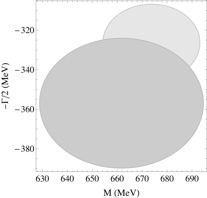
Figure 1: Upper panel, uncertainty $\Delta\sqrt{s_{p}^{N}}$ for different values of $\sqrt{s_{0}}$ in the $\kappa$ pole determination for M=1. We show dotted and dashed lines for N=2 and N=3 respectively. It is clear that the M=1 case does not converge as N increases. We have checked higher $N$ and there is no improvement. Lower panel, theoretical uncertainty regions $\Delta\sqrt{s_{p}^{N}}$ for the best center $\sqrt{s_{0}}$ for M=1, where N=2 is plotted as the light gray region and N=3 as the gray region.

The results for $M=1$ can be found in Fig. 1. In the upper panel we show $\Delta\sqrt{s_{p}^{N}}$ for different values of $s_{0}$. Note that the $N=3$ curve (dashed) is nowhere smaller then that of $N=2$ (dotted). The smallest uncertainty for each $N$ is attained at $\sqrt{s_{0}}\sim 830\,$MeV, and we show in the lower panel how it translates into a truncation uncertainty for the pole position, which grows from $N=2$ (light gray circle) to $N=3$ (darker gray circle). Note also that the central value of the darker circle lies well outside the lighter circle. We have also calculated the $N=4,5$ cases and there is no evidence of convergence for $M=1$. We thus conclude that considering the Padé series with just one pole is not enough to reproduce the analytic structure in the region relevant for such a deep pole.

We then show in Fig. 2 the results for the $M=2$ Padé series, which has two poles. Once again, in the upper panel we show $\Delta\sqrt{s_{p}^{N}}$, for different values of $s_{0}$, as dotted and dashed curves for $N=2$ and $N=3$, respectively. Now we see that this truncation difference decreases drastically in several $s_{0}$ regions as $N$ increases. Actually, already at $N=3$ it becomes smaller than the statistical uncertainties, with a minimum at $\sqrt{s_{0}}=950\,$MeV. Thus the $P^{3}_{2}$ pole will define our resonance values and $\Delta\sqrt{s_{p}^{3}}$ the theoretical uncertainty $\Delta_{th}$ listed in Table 1. In the lower panel we show the pole position and its minimum truncation uncertainty for $N=2,3$ as the light and dark gray areas, respectively. The other pole obtained for this sequence corresponds to the $\eta K$ threshold, which is the nearest singularity to $s_{0}$.

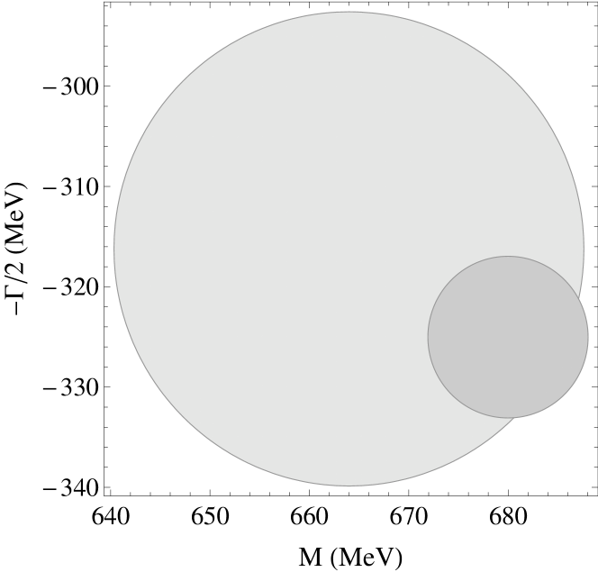
Figure 2: Upper panel, uncertainty $\Delta\sqrt{s_{p}^{N}}$ for different values of $\sqrt{s_{0}}$ in the $\kappa$ pole determination for M=2. We show dotted and dashed lines for N=2 and N=3 respectively. Lower panel, theoretical uncertainty regions $\Delta\sqrt{s_{p}^{N}}$ for the best center $\sqrt{s_{0}}$ for M=2, where N=2 is plotted as the light gray region and N=3 as the gray region.

Once a central value and a theoretical error for the pole position has been obtained, we add the statistical uncertainty in quadrature:

$$\Delta_{s_{p}}=\sqrt{\Delta_{th}^{2}+\Delta_{stat}^{2}}.$$ (8)

Recall that the statistical errors are obtained from a Monte Carlo Gaussian sampling of the parameters of the CFD parameterization within their uncertainties. Statistical uncertainties dominate the quadrature, since the theoretical error is the $\Delta\sqrt{s_{p}^{N}}$ for the $N$ when it becomes smaller than the experimental one. In the case of the $K^{*}(800)$ this procedure leads to the results for the pole position and the coupling that are listed in the second column of Table 1. The central value $(680\pm 13)-i(325\pm 7)\,$MeV obtained with the Padé approximant can now be compared with the pole position extracted analytically from the CFD parameterization in $(680\pm 15)-i(334\pm 7.5)\,$MeV. This illustrates the remarkable accuracy of the Padé sequence to extract resonance parameters and the soundness of our method to estimate uncertainties.

Table 1: $K_{0}^{*}(800)$ pole results for the CFD and different parameterizations fitted to the CFD. The uncertainty for $\sqrt{s_{p}}$ and $g$ include statistical and theoretical errors only.

	CFD Padé	Schenk Padé	C-M Padé
$\sqrt{s_{p}}$(MeV)	(680$\pm$13)-$i$(325$\pm$7)	(656)-$i$(283)	(673)-$i$(276)
$\Delta_{th}$(MeV)	6	13	10
$g$(GeV)	4.88$\pm$0.16	4.30	4.22
$\Delta_{th}$(GeV)	0.15	0.32	0.20
$\sqrt{s_{0}}$(GeV)	0.96	0.81	0.87

In the third and fourth columns of Table 1 we also show the results obtained by following the same procedure with the Schenk Schenk:1991xe and Chew-Mandelstam (C-M) Chew:1960iv parameterizations already used in Caprini:2016uxy fitted to the CFD curve. For each parameterization we choose its best $s_{0}$ value. As explained above, although these parameterizations fall within the uncertainties of the CFD in the real axis, they yield slightly different derivatives, which result in somewhat different values for the pole. Thus, we take as our final central result for the $K_{0}^{*}(800)$ resonance the average of these different parameterizations and consider the systematic uncertainty as explained in the introduction, combining it quadratically with the theoretical and statistical uncertainties. We thus arrive to the final result for the $K_{0}^{*}(800)$ pole and coupling:

$$\sqrt{s_{K_{0}^{*}(800)}} = (670\pm 18)-i(295\pm 28)\;{\rm MeV},$$ (9)

$$g_{K_{0}^{*}(800)} = 4.47\pm 0.40\;{\rm GeV}.$$

This result is shown in Fig.3 together with the other references listed in the RPP for this resonance. Note that we have highlighted with solid symbols those poles coming from analytic or dispersive approaches, whereas mass and width values obtained from models using Breit-Wigner approximations are shown with empty squares.

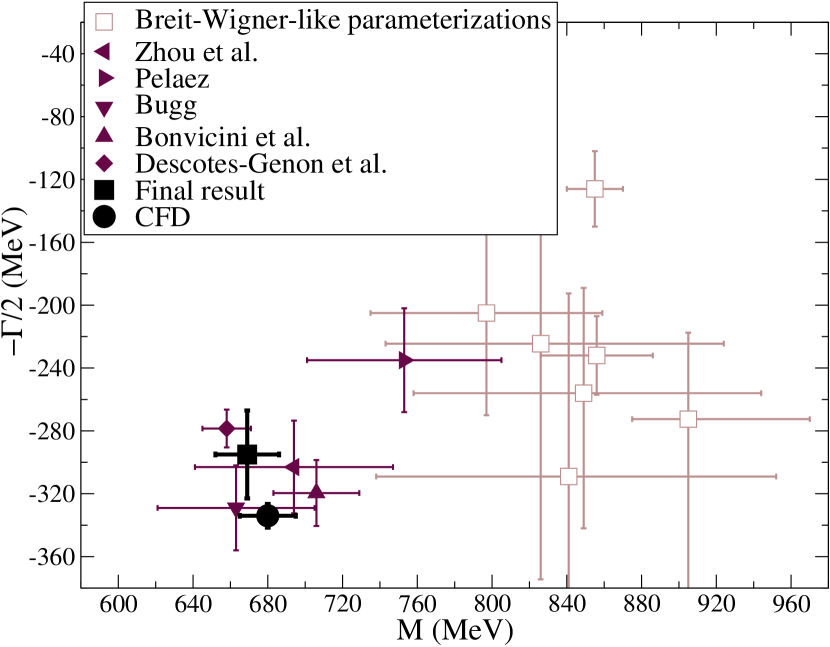
Figure 3: Final result for the $\kappa$ pole. Other references are taken from the RPP compilation PDG , Descotes-Genon et al. DescotesGenon:2006uk , Bonvicini et al. Bonvicini:2008jw , D.Bugg Bugg:2003kj , J.R.Peláez GomezNicola:2001as , Zhou et al. Zhou:2006wm , and the Breit-Wigner parameterizations Ablikim:2010ab listed in the RPP.

4.1.2 The $K_{0}^{*}(1430)$

For the heavier $K_{0}^{*}(1430)$ resonance, the elastic formalism cannot be used, although the resonance is almost elastic, since its branching ratio to $\pi K$ is larger than $90\%$. In this case the CFD Pelaez:2016tgi makes use of and inelastic formalism parameterized through simple rational functions that fit the total phase and the modulus of the partial wave. Let us remark that, even for $\pi\pi$ scattering, no partial-wave dispersion relations have been implemented up to more than 1.1 GeV, since Roy and GKPY equations reach 1.1 GeV at most in their usual formulation. Forward dispersion relations have been extended for $\pi\pi$ scattering up to 1420 MeV GarciaMartin:2011cn and for $K\pi$ up to 1600 MeV Pelaez:2016tgi , but they are not suitable for resonance pole extractions. Therefore, lacking these rigorous dispersive methods to extract poles, it is here where the Padé technique yields more relevant results, providing a sound analytic continuation to the next Riemann sheet.

The convergence of the $P^{N}_{1}$ sequence, with just one pole, is fairly good this time because the resonance is not as deep in the complex plane as the $K_{0}^{*}(800)$. In particular, the truncation errors, shown in the upper panel of Fig. 4 decrease from $N=2$ to $4$ rather fast for $s_{0}$ within the $1350-1420$ MeV range. We obtain a minimum for the combined $\Delta_{s_{p}}$ error at $\sqrt{s_{0}}=1380$ MeV. Once more, the Padé series has been truncated at $N=4$, where the theoretical error becomes smaller than the statistical one calculated from a Monte Carlo Gaussian sampling of the CFD parameters. This truncation uncertainty translates into the light gray, gray and dark gray areas in the lower panel of Fig. 4. The darker one gives our final central value and theoretical uncertainty, whose numerical values can be read in the second column of Table 2. In addition, we have added in quadrature the statistical uncertainty in the first line.

In that Table we also show the result of using a typical Breit-Wigner model, as done in most of the works listed in the RPP, to fit the CFD parameterization. As it can be seen in the third column of Table 2, this leads to a sizable change in the width, but to almost an imperceptible variation of the mass. This is a source of systematic uncertainty due to model dependence. Our final result is obtained by combining the three sources of uncertainty: theoretical, statistical, and systematic. We find

$$\sqrt{s_{K_{0}^{*}(1430)}} = (1431\pm 6)-i(110\pm 19)\;{\rm MeV},$$ (10)

$$g_{K_{0}^{*}(1430)} = 3.82\pm 0.74\;{\rm GeV}.$$

In Fig. 5 we have plotted this final result value as a black circle, which compares rather well with the references listed in the RPP.

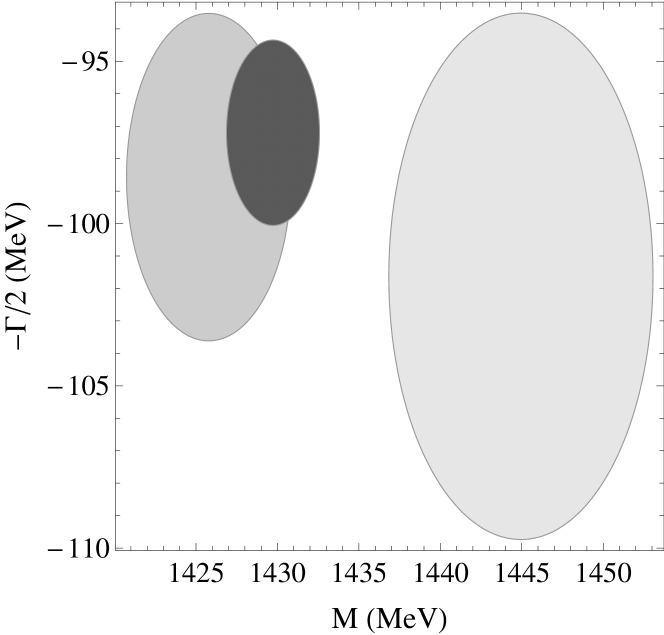
Figure 4: Upper panel, uncertainty $\Delta\sqrt{s_{p}^{N}}$ for different values of $\sqrt{s_{0}}$ in the $K_{0}^{*}(1430)$ pole determination. The dotted, dashed and continuous lines correspond to the $N=2,3$ and 4 cases, respectively. Lower panel, theoretical uncertainty regions $\Delta\sqrt{s_{p}^{N}}$ for the $K_{0}^{*}(1430)$ pole. The light gray, gray and dark grey areas correspond to $N=2,3$ and 4.

Table 2: $K_{0}^{*}(1430)$ pole results for the CFD and different parameterizations fitted to the CFD. The uncertainty for $\sqrt{s_{p}}$ and $g$ include statistical and theoretical errors only.

	CFD Padé	BW Padé
$\sqrt{s_{p}}$(MeV)	(1430$\pm$5)-$i$(97$\pm$6)	(1431)-$i$(122)
$\Delta_{th}$(MeV)	3	7
$g$(GeV)	3.31$\pm$0.21	4.32
$\Delta_{th}$(GeV)	0.06	0.07
$\sqrt{s_{0}}$(GeV)	1.38	1.44

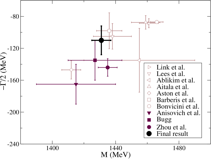
Figure 5: Final result for the $K_{0}^{*}(1430)$ pole. Other results correspond to those listed in the RPP compilation PDG , Zhou et al. Zhou:2006wm , D.Bugg Bugg:2003kj , Anisovich et al. Anisovich:1997qp , Bonvicini et al. Bonvicini:2008jw , Barberis et al. Barberis:1998tv , Aston et al. Aston:1987ir , Aitala et al. Ablikim:2010ab , Ablikim et al. Ablikim:2005kp , Lees et al. Lees:2014iua , Link et al. Pennington:2007se .

4.2 Vector resonances

Let us now discuss the vector resonances that appear in $K\pi$ scattering below 1.8 GeV. These are the $K^{*}(892)$ and the $K_{1}^{*}(1410)$, both of them with isospin $1/2$.

4.2.1 The $K^{*}(892)$

The lightest one is the $K^{*}(892)$, which is elastic for all means and purposes. It is also very narrow compared to the $K_{0}^{*}(800)$ and therefore much closer to the real axis and well isolated from other analytic structures. Hence, as can be seen in the upper panel of Fig. 6, the $P^{N}_{1}$ sequence, with just one pole, converges very rapidly. Actually, we estimate our theoretical error from $N=4$ since it is when the truncation error becomes negligible compared to the statistical one (four orders of magnitude smaller), obtained as usual from a Monte Carlo Gaussian sampling of the CFD parameters. The $\Delta_{s_{p}}$ error is minimized for $\sqrt{s_{0}}=890$ MeV, but the outcome is remarkably similar within the $870-910$ MeV range. In the lower panel of Fig. 6 we see that the theoretical uncertainty on the pole becomes extremely small and that he convergence is remarkable, with the central value being almost the same from $N=2$ to $N=4$.

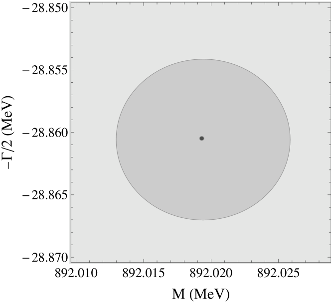
Figure 6: Upper panel: $\Delta\sqrt{s_{p}^{N}}$ in the $K^{*}(892)$ pole determination for different values of $\sqrt{s_{0}}$ using the $P_{1}^{N}$ sequence. The dotted, dashed and continuous lines correspond to $N=2,3$ and 4, respectively. Lower panel: theoretical uncertainty regions $\Delta\sqrt{s_{p}^{N}}$ for the $K^{*}(892)$ pole. The light gray and gray areas correspond to $N=2,3$, whereas the $N=4$ case corresponds to the tiny dark gray spot in the center, since the theoretical uncertainty becomes negligible.

Concerning the systematic uncertainty due to the use of other models to fit the same data, we have found that the result, if we consider a Breit-Wigner model fitted to the CFD values, differs by less than $1$ MeV. However, it is worth noting that when fitting a Breit-Wigner to the CFD result, the sequence of Padé approximants with just one pole converges rather poorly. We have also tried other conformal parameterizations with different centers. In any case, by changing the model, the systematic uncertainty is smaller than the statistical error, which dominates the uncertainty in our final result.

The final result for the $K^{*}(892)$ parameters is shown in Table 3. This result may appear incompatible with the determinations in the RPP. There are several reasons for this: first, because in the RPP only Breit-Wigner (BW) parameters are given and then $s_{p}=M_{BW}^{2}-iM_{BW}\Gamma_{BW}$, so that $\mathrm{Re}\,\sqrt{s_{p}}$ is not exactly $M_{BW}$ and $\mathrm{Im}\,\sqrt{s_{p}}$ is not exactly $\Gamma_{BW}/2$. Taking these different definitions into account improves slightly the agreement. Second, there is the issue of using an isospin conserving formalism when extracting the CFD parameterization and when measuring the data, so that our resonances do not correspond to the charged nor the neutral cases. Therefore, when comparing to the resonances observed in a charged or neutral channels, which are the ones listed in the PDG, a difference of about $\pm 2\,$MeV is expected to arise. However, our pole is to be understood as the pole in the isospin conserving limit. Note that this distinction between charges and neutral resonances is not done in the RPP for other resonances. Moreover, there is a third reason, which is that the BW extractions of resonance parameters are usually obtained from a fit to the amplitude in a limited region or assuming the existence of a certain background from other regions or resonances. In contrast, here the whole elastic region is described with the CFD amplitude, thus, we are giving the pole of the whole amplitude. In general we do not think that obtaining this particular resonance from scattering data is competitive with the determinations from other reactions, which much better data and statistics.

Table 3: $K^{*}(892)$ pole results. The uncertainty for $\sqrt{s_{p}}$ and $g$ include statistical and theoretical errors only.

	CFD Padé
$\sqrt{s_{p}}$(MeV)	(892$\pm$1)-$i$(29$\pm$1)
$\Delta_{th}$(MeV)	1$\cdot{10^{-4}}$
$g$	6.1$\pm$0.1
$\Delta_{th}$	$\simeq$0
$\sqrt{s_{0}}$(GeV)	0.89

4.2.2 The $K_{1}^{*}(1410)$

Let us now turn to the $K_{1}^{*}(1410)$, which cannot be considered elastic and has a rather small $7\%$ branching fraction to $K\pi$. Still, we will be able to obtain its pole, as we did for the $K_{0}^{*}(1430)$, since Padé approximants also provide the analytic continuation to the continuous Riemann sheet of the partial waves in the inelastic region. Once more it is enough to compute derivatives from the vector partial-wave CFD parameterization in Pelaez:2016tgi .

The theoretical convergence is really fast as can be observed in Fig. 7. The theoretical error is small in the range $1280-1450\,$MeV, with a minimum for the total error located at $\sqrt{s_{0}}=1304$ MeV. In this case the theoretical uncertainty becomes much smaller than the statistical one at $N=4$. Partly, this is due to the fact that in this energy region there are two conflicting experiments and this leads to large uncertainties in the CFD parameterization. As a consequence, what we call “statistical” uncertainties dominate the final result for this resonance.

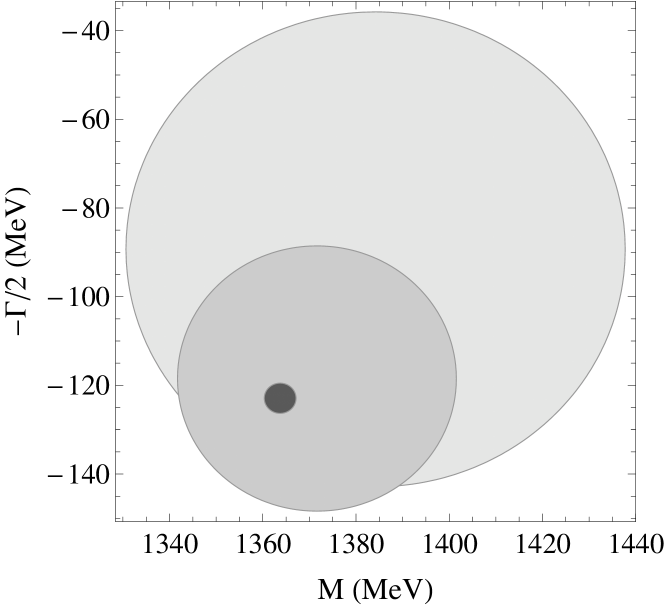
Figure 7: Upper panel: $\Delta\sqrt{s_{p}^{N}}$ in the $K_{1}^{*}(1410)$ pole determination for different values of $\sqrt{s_{0}}$ using the $P_{1}^{N}$ sequence. The dotted, dashed and continuous lines correspond to $N=2,3$ and 4, respectively. Lower panel: theoretical uncertainty regions $\Delta\sqrt{s_{p}^{N}}$ for the $K_{1}^{*}(1410)$ pole. The light gray, gray and dark gray areas correspond to $N=2,3$ and 4.

As with other resonances, we have also fitted other parameterizations to the CFD data to estimate the systematic uncertainty when calculating the derivatives at one given energy. In Table 4 we show the results when calculating the derivatives with a BW formalism, which is the one used by all the determinations quoted in the RPP PDG . For the final central value we thus take the average over these two determinations and we evaluate our final error as the quadrature between statistical, theoretical, and systematic uncertainties as:

$$\sqrt{s_{K_{1}^{*}(1410)}} = (1368^{+38}_{-38})-i(106^{+48}_{-59})\;{\rm MeV},$$ (11)

$$g_{K_{1}^{*}(1410)} = 1.89^{+1.77}_{-1.34}.$$

This might look less precise than the averaged result of $M=1414\pm 15\,$MeV and $\Gamma/2=116\pm 10.5$ given in the RPP PDG , but this is because this average is dominated by a measurement of the LASS experiment on $K^{-}p\rightarrow\bar{K}^{0}\pi^{+}\pi^{-}n$ Aston:1986rm using a BW parameterization with simple backgrounds. It is not evident the systematic effect due to these simple backgrounds. When using the $K\pi$ scattering data obtained later by the same experiment Aston:1987ir one obtains $M=1380\pm 21\pm 19$ and $\Gamma/2=88\pm 26\pm 11$, very similar to our extraction, but based only on a BW formalism and without taking into account the conflicting data of Estabrooks et al. Estabrooks:1977xe in this region. In this sense we think our result is more robust and confirms the parameters of this resonance without using a specific BW functional form, nor assuming any particular background. In Fig. 8 we show how our final result compares to all other results listed in the RPP. It can be seen that the results are rather consistent with the exception of that of Etkin et al. Etkin:1980me .

Table 4: $K_{1}^{*}(1410)$ pole results for the CFD and different parameterizations fitted to the CFD. The uncertainty for $\sqrt{s_{p}}$ and $g$ include statistical and theoretical errors only.

	CFD Padé	BW Padé
$\sqrt{s_{p}}$(MeV)	$(1362^{+37}_{-37})-$i$(123^{+41}_{-54})$	$(1374)-$i$(88)$
$\Delta_{th}$(MeV)	3	0.7
$g$	$2.41^{+1.60}_{-1.11}$	1.36
$\Delta_{th}$	0.04	0.007
$\sqrt{s_{0}}$(GeV)	1.30	1.38

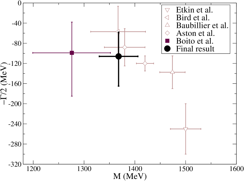
Figure 8: Final result for the $K_{1}^{*}(1410)$ pole. Other references are taken from the RPP compilation PDG , Boito et al. Boito:2008fq , Aston et al. Aston:1987ir , Baubillier et al. Baubillier:1982eb , Bird et al. Bird:1988qp , Etkin et al. Etkin:1980me .

4.3 Tensor resonances

In practice, once we reach 1.3 GeV all available channels have some measured inelasticity. Since all resonances with $J=2$ or higher angular momentum waves are above this energy, we use the inelastic CFD parameterization of Pelaez:2016tgi and the fact that the Padé approximants perform the analytical continuation directly to the continuous Riemann sheet. We describe next how we extract the parameters of the $K_{2}^{*}(1430)$ and $K_{3}^{*}(1780)$ resonances, which have $J=2$ and 3 respectively.

4.3.1 The $K_{2}^{*}(1430)$

This resonance appears in $K\pi$ scattering with angular momentum $2$ and isospin $1/2$ and shows a nice Breit-Wigner-like shape. Its branching ratio to $K\pi$ is $50\%$, the other relevant channels being $K^{*}(892)\pi$, $K^{*}(892)\pi\pi$ and $K\rho$.

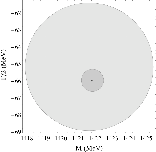
Figure 9: Upper panel: $\Delta\sqrt{s_{p}^{N}}$ in the $K_{2}^{*}(1430)$ pole determination for different values of $\sqrt{s_{0}}$ using the $P_{1}^{N}$ sequence. The dotted, dashed and continuous lines correspond to $N=2,3$ and 4, respectively. Lower panel: theoretical uncertainty regions $\Delta\sqrt{s_{p}^{N}}$ for the $K_{2}^{*}(1430)$ pole. The light gray, gray and dark gray areas correspond to $N=2,3$ and 4.

Since there is a well isolated pole, we can use the $M=1$ Padé sequence with one pole. The upper panel of Fig. 9 shows how the sequence converges rapidly and for $N=4$ the truncation uncertainty is completely negligible, having a minimum at $\sqrt{s_{0}}=1410$ MeV. In the lower panel we see that the area covered by the $N=4$ Padé, almost becomes a point and that the central value of the pole position is very stable. The parameters of the resonance thus obtained are listed in Table 5.

Table 5: $K_{2}^{*}(1430)$ pole results for the CFD and different parameterizations fitted to the CFD. The uncertainty for $\sqrt{s_{p}}$ and $g$ include statistical and theoretical errors only.

	CFD Padé	BW Padé
$\sqrt{s_{p}}$(MeV)	(1422$\pm$3)-$i$(66$\pm$2)	(1427)-$i$(66)
$\Delta_{th}$(MeV)	0.04	0.01
$g$(GeV)-1	3.37$\pm$0.07	3.08
$\Delta_{th}$(GeV)-1	0.001	$3\times 10^{-5}$
$\sqrt{s_{0}}$(GeV)	1.41	1.51

As done with other resonances, we have tried calculating the derivatives needed for the Padé approximants by means of other parameterizations fitted to the CFD results. In particular we show in Table 5 the result when using a Breit-Wigner formula fitted to the CFD and then the Padé approximants to extract the pole. The difference is rather small, but we have taken the average with the CFD result obtained with Padés and added the systematic uncertainty as explained in the introduction, yielding our final result:

$$\sqrt{s_{K_{2}^{*}(1430)}} = (1424\pm 4)-i(66\pm 2)\;{\rm MeV},$$ (12)

$$g_{K_{2}^{*}(1430)} = 3.23\pm 0.22\;{\rm GeV}^{-1},$$

which, as can be seen in Fig. 10 is in good agreement with other determinations quoted in the RPP PDG . The RPP average is dominated by the work of LASS Aston:1986rm ; Aston:1987ir , which use BW formalisms and simple backgrounds. Our result has a relatively small uncertainty despite including estimates of systematic error, both in the pole extraction and the data, and avoiding the use of backgrounds or other assumptions in the pole extraction.

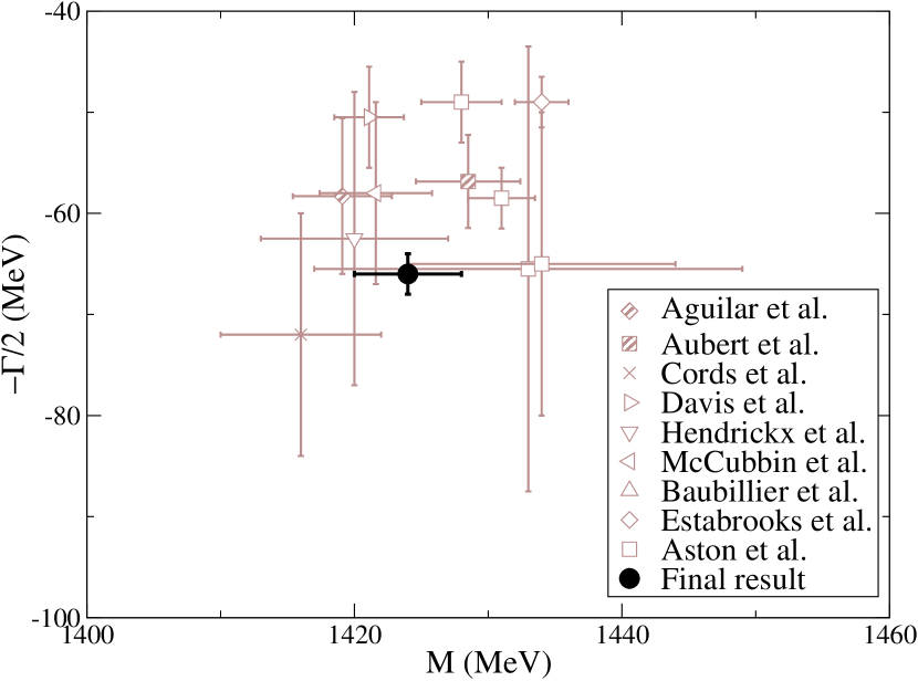
Figure 10: Final result for the $K_{2}^{*}(1430)$ pole. The following references are taken from the RPP compilation PDG , Aston et al. Aston:1987ir , Estabrooks et al. Estabrooks:1977xe , Baubillier et al. Baubillier:1982eb , Mccubbin et al. McCubbin:1974yy , Hendrickx et al. Hendrickx:1976ha , Davis et al. Davis:1969sf , Cords et al. Cords:1972hh , Aubert et al. Aubert:2007ur , Aguilar et al. AguilarBenitez:1972bw .

4.3.2 The $K_{3}^{*}(1780)$

The heaviest strange resonance that can be studied using the CFD parameterizations is the $K_{3}^{*}(1780)$, which appears in the $F$-wave with isospin 1/2. Let us note that the $K_{3}^{*}(1780)$ has a branching ratio to $\pi K$ of $20\%$, with the other 3 relevant channels being $K\rho$, $K^{*}(892)$ and $K\eta$. First of all, let us remark that its mass lies beyond 1600 MeV, the energy up to which the CFD parameterization satisfies well the Forward Dispersion Relations. Nevertheless, as explained in Pelaez:2016tgi , this is most likely due to the data in other waves, since imposing FDRs up to higher energies demands deviations from the $D$-wave data, for instance, but the $F$-wave barely changes from an unconstrained fit up to larger energies. Thus we feel confident our method can be applied to this resonance.

The $K_{3}^{*}(1780)$ is well isolated from contributions from other singularities and we can use the Padé sequence with just one pole. As usual, we show in Fig. 11 the convergence of the sequence which has a very small truncation error for $N=4$. Actually, it is about two orders of magnitude smaller than the statistical one, as seen in Table 11. As seen in the lower panel of that figure, the central value barely changes with $N$ (Note the small scale of the axis).

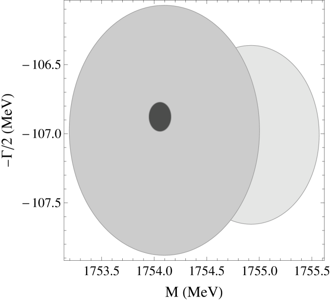
Figure 11: Upper panel: $\Delta\sqrt{s_{p}^{N}}$ in the $K_{3}^{*}(1780)$ pole determination for different values of $\sqrt{s_{0}}$ using the $P_{1}^{N}$ sequence. The dotted, dashed and continuous lines correspond to $N=2,3$ and 4, respectively. Lower panel: theoretical uncertainty regions $\Delta\sqrt{s_{p}^{N}}$ for the $K_{3}^{*}(1780)$ pole. The light gray, gray and dark gray areas correspond to $N=2,3$ and 4.

Once again we have tried to estimate the uncertainty due to calculating the derivatives of the amplitude with different parameterizations, but the differences are rather small. In Table 11 we show the pole extracted with the Padé method if, instead of using the CFD parameterizations, we use a BW fit to the CFD. The mass and width barely change but the coupling is slightly different, changing by less than the statistical uncertainty. We thus take the average and enlarge the uncertainty with a systematic error combined as explained in the introduction to this section. Our result is:

$$\sqrt{s_{K_{3}^{*}(1780)}} = (1754\pm 13)-i(119\pm 14)\;{\rm MeV},$$ (13)

$$g_{K_{3}^{*}(1780)} = 1.28\pm 0.14\;{\rm GeV}^{-2},$$

which, as seen in Fig. 12 is compatible with the results quoted in the RPP PDG . It should be noted that our uncertainties are only slightly larger than the RPP average, which is dominated by the result of Aston et al. Aston:1987ir , but here we do not make a particular assumption for the functional form or a background in the amplitude.

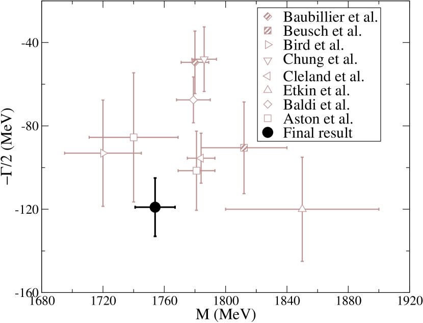
Figure 12: Final result for the $K_{3}^{*}(1780)$ pole determination. We also show a are taken from the PDG PDG , Aston et al. Aston:1987ir , Baldi et al. Baldi:1976ua , Etkin et al. Etkin:1980me , Cleland et al. Cleland:1982td , Chung et al. Chung:1977ji , Bird et al. Bird:1988qp , Beusch et al. Konigs:1978at , Baubillier et al. Baubillier:1982eb .

Table 6: $K_{3}^{*}(1780)$ pole results for the CFD and different parameterizations fitted to the CFD. The uncertainty for $\sqrt{s_{p}}$ and $g$ include statistical and theoretical errors only.

	CFD Padé	BW Padé
$\sqrt{s_{p}}$(MeV)	(1753$\pm$13)-$i$(119$\pm$14)	(1755)-$i$(118)
$\Delta_{th}$(MeV)	0.3	4.3
$g$(GeV)-2	1.32$\pm$0.13	1.23
$\Delta_{th}$(GeV)-2	0.003	0.03
$\sqrt{s_{0}}$(GeV)	1.73	1.76

5 Summary

In this work we have presented a determination of the parameters of resonances that appear in $K\pi$ scattering below 1.8 GeV. This has been achieved by means of series of Padé approximants, which should converge to the appropriate analytic structure of the amplitude in a given domain. This constitutes another instance of the applicability and usefulness of this method, which avoids specific model assumptions in the determinations of the mass, width, and coupling of a resonance. As a matter of fact, these parameters are usually obtained from Breit-Wigner-like parameterizations (or slight modifications) which make a specific relation between the width and residue, and usually assume that the data contain simple backgrounds superimposed to the resonance signal. With this method we determine the pole without such assumptions. Moreover, it should be remarked that this method can be applied in the inelastic region, where the powerful partial-wave dispersion relations cannot be used in practice to obtained poles.

In addition, these determinations have been obtained using as input a recent dispersive description of all the $K\pi$ data, which is constrained to satisfy two Forward Dispersion Relations (and several crossing sum rules) up to 1600 MeV. It should also be noted that simple fits to the data, as those used in previous determinations of resonance parameters, do not fulfill these fundamental constraints. These constrained fits have also taken into account systematic uncertainties due to incompatibilities between different experiments.

Thus, we have provided determinations of the mass, width and coupling to $K\pi$ for the conflictive $K_{0}^{*}(800)$ or $\kappa$ resonance, the $K_{0}^{*}(1430)$ scalar, the $K^{*}(892)$ and $K_{1}^{*}(1410)$ vectors, the spin-two $K_{2}^{*}(1430)$ as well as the spin-three $K^{*}_{3}(1780)$. The results are fairly competitive with the results on the Review of Particle Properties, although it should be noted that these results contain some estimation of systematic and theoretical uncertainties usually lacking in the literature.

References

- (1) D. Aston et al., Phys. Lett. B 180, 308 (1986) Erratum: [Phys. Lett. B 183, 434 (1987)].
- (2) C. Patrignani et al. (Particle Data Group), Chin. Phys. C, 40, 100001 (2016).
- (3) B. Ananthanarayan, G. Colangelo, J. Gasser and H. Leutwyler, Phys. Rept. 353, 207 (2001).
- (4) P. Buettiker, S. Descotes-Genon and B. Moussallam, Eur. Phys. J. C 33, 409 (2004).
- (5) R. Garcia-Martin, R. Kaminski, J. R. Pelaez, J. Ruiz de Elvira and F. J. Yndurain, Phys. Rev. D 83, 074004 (2011).
- (6) M. Hoferichter, J. Ruiz de Elvira, B. Kubis and U. G. Meißner, Phys. Rept. 625, 1 (2016).
- (7) S. M. Roy, Phys. Lett. 36B, 353 (1971). I. Caprini, G. Colangelo and H. Leutwyler, Phys. Rev. Lett. 96 (2006) 132001 B. Moussallam, Eur. Phys. J. C 71, 1814 (2011)
- (8) R. Garcia-Martin, R. Kaminski, J. R. Pelaez and J. Ruiz de Elvira, Phys. Rev. Lett. 107 (2011) 072001
- (9) J. R. Pelaez, Phys. Rept. 658, 1 (2016)
- (10) S. Descotes-Genon and B. Moussallam, Eur. Phys. J. C 48 (2006) 553
- (11) S. N. Cherry and M. R. Pennington, Nucl. Phys. A 688, 823 (2001)
- (12) F. J. Yndurain, R. Garcia-Martin and J. R. Pelaez, Phys. Rev. D 76 (2007) 074034
- (13) I. Caprini, Phys. Rev. D 77 (2008) 114019
- (14) Z. H. Guo and J. A. Oller, Phys. Rev. D 93 (2016) no.9, 096001 J. A. Oller, Phys. Rev. D 71 (2005) 054030
- (15) A. varc, et. al Phys. Rev. C 88, no. 3, 035206 (2013) Phys. Rev. C 89 (2014) no.4, 045205 Phys. Rev. C 89, no. 6, 065208 (2014) Phys. Rev. C 89, no. 6, 065208 (2014)
- (16) P. Masjuan and J. J. Sanz-Cillero, Eur. Phys. J. C 73, 2594 (2013)
- (17) P. Masjuan, J. Ruiz de Elvira and J. J. Sanz-Cillero, Phys. Rev. D 90, no. 9, 097901 (2014)
- (18) I. Caprini, P. Masjuan, J. Ruiz de Elvira and J. J. Sanz-Cillero, Phys. Rev. D 93, no. 7, 076004 (2016)
- (19) J. R. Pelaez and A. Rodas, Phys. Rev. D 93, no. 7, 074025 (2016)
- (20) P. Estabrooks et al., Nucl. Phys. B 133, 490 (1978).
- (21) D. Aston et al., Nucl. Phys. B 296, 493 (1988).
- (22) E. van Beveren, T. A. Rijken, K. Metzger, C. Dullemond, G. Rupp and J. E. Ribeiro, Z. Phys. C 30 (1986) 615
- (23) A. Dobado and J. R. Pelaez, Phys. Rev. D 47, 4883 (1993) Phys. Rev. D 56, 3057 (1997)
- (24) A. Gomez Nicola and J. R. Pelaez, Phys. Rev. D 65, 054009 (2002). J. R. Pelaez, Mod. Phys. Lett. A 19, 2879 (2004)
- (25) H. Q. Zheng, Z. Y. Zhou, G. Y. Qin, Z. Xiao, J. J. Wang and N. Wu, Nucl. Phys. A 733, 235 (2004)
- (26) J. A. Oller, E. Oset and J. R. Pelaez, Phys. Rev. Lett. 80, 3452 (1998) Phys. Rev. D 59 (1999) 074001 Erratum: [Phys. Rev. D 60 (1999) 099906] Erratum: [Phys. Rev. D 75 (2007) 099903] J. A. Oller and E. Oset, Phys. Rev. D 60, 074023 (1999)
- (27) D. Black, A. H. Fariborz, F. Sannino and J. Schechter, Phys. Rev. D 58, 054012 (1998) Phys. Rev. D 59, 074026 (1999)
- (28) M. Jamin, J. A. Oller and A. Pich, Nucl. Phys. B 587, 331 (2000)
- (29) T. Wolkanowski, M. So tysiak and F. Giacosa, Nucl. Phys. B 909, 418 (2016)
- (30) T. Ledwig, J. Nieves, A. Pich, E. Ruiz Arriola and J. Ruiz de Elvira, Phys. Rev. D 90, no. 11, 114020 (2014).
- (31) S. Ishida, M. Ishida, T. Ishida, K. Takamatsu and T. Tsuru, Prog. Theor. Phys. 98, 621 (1997)
- (32) D. V. Bugg, Phys. Lett. B 572, 1 (2003) Erratum: [Phys. Lett. B 595, 556 (2004)]. Phys. Rev. D 81, 014002 (2010)
- (33) P. C. Magalhaes and M. R. Robilotta, Phys. Rev. D 90 (2014) no.1, 014043
- (34) R. Navarro Pérez, E. Ruiz Arriola and J. Ruiz de Elvira, Phys. Rev. D 91, 074014 (2015)
- (35) T. N. Truong, Phys. Rev. Lett. 61, 2526 (1988). A. Dobado, M. J. Herrero and T. N. Truong, Phys. Lett. B 235, 134 (1990).
- (36) A. Dobado and J. R. Pelaez, Phys. Rev. D 56, 3057 (1997) A. Dobado and J. R. Pelaez, Phys. Rev. D 47, 4883 (1993)
- (37) J. Gasser and U. G. Meissner, Nucl. Phys. B 357, 90 (1991).
- (38) G. Bonvicini et al. [CLEO Collaboration], Phys. Rev. D 78, 052001 (2008)
- (39) Z. Y. Zhou and H. Q. Zheng, Nucl. Phys. A 775, 212 (2006)
- (40) M. Ablikim et al. [BES Collaboration], Phys. Lett. B 698, 183 (2011) M. Ablikim et al., Phys. Lett. B 693, 88 (2010) M. Ablikim et al. [BES Collaboration], Phys. Lett. B 633, 681 (2006) E. M. Aitala et al. [E791 Collaboration], Phys. Rev. Lett. 89, 121801 (2002) C. Cawlfield et al. [CLEO Collaboration], Phys. Rev. D 74, 031108 (2006) S. Ishida, M. Ishida, T. Ishida, K. Takamatsu and T. Tsuru, Prog. Theor. Phys. 98, 621 (1997) J. M. Link et al. [FOCUS Collaboration], Phys. Lett. B 535, 43 (2002)
- (41) A. Schenk, Nucl. Phys. B 363, 97 (1991).
- (42) G. F. Chew and S. Mandelstam, Phys. Rev. 119 (1960) 467.
- (43) A. V. Anisovich and A. V. Sarantsev, Phys. Lett. B 413, 137 (1997)
- (44) D. Barberis et al. [WA102 Collaboration], Phys. Lett. B 436, 204 (1998)
- (45) M. Ablikim et al. [BES Collaboration], Phys. Rev. D 72, 092002 (2005)
- (46) J. P. Lees et al. [BaBar Collaboration], Phys. Rev. D 89, no. 11, 112004 (2014)
- (47) J. M. Link et al. [FOCUS Collaboration], Phys. Lett. B 653, 1 (2007)
- (48) D. R. Boito, R. Escribano and M. Jamin, Eur. Phys. J. C 59, 821 (2009)
- (49) M. Baubillier et al. [BIRMINGHAM-CERN-GLASGOW-MICHIGAN STATE-PARIS Collaboration], Nucl. Phys. B 202, 21 (1982). M. Baubillier et al. [Birmingham-CERN-Glasgow-Michigan State-Paris Collaboration], Z. Phys. C 26, 37 (1984).
- (50) F. P. Bird, SLAC-0332, SLAC-332, UMI-89-12872, SLAC-R-0332, SLAC-R-332.
- (51) A. Etkin et al., Phys. Rev. D 22, 42 (1980).
- (52) N. A. McCubbin and L. Lyons, Nucl. Phys. B 86, 13 (1975).
- (53) K. Hendrickx, P. Cornet, F. Grard, V. P. Henri, R. Windmolders, D. Vignaud, D. Burlaud and S. Tavernier, Nucl. Phys. B 112, 189 (1976).
- (54) P. J. Davis, S. E. Derenzo, S. M. Flatte, M. Alston-Garnjost, G. R. Lynch and F. T. Solmitz, Phys. Rev. Lett. 23, 1071 (1969).
- (55) D. Cords et al., Phys. Rev. D 4, 1974 (1971).
- (56) B. Aubert et al. [BaBar Collaboration], Phys. Rev. D 76, 012008 (2007)
- (57) M. Aguilar-Benitez, R. L. Eisner and J. B. Kinson, Phys. Rev. D 4, 2583 (1971).
- (58) R. Baldi et al., Phys. Lett. 63B, 344 (1976).
- (59) W. e. Cleland et al., Nucl. Phys. B 208, 189 (1982).
- (60) S. U. Chung et al., Phys. Rev. Lett. 40, 355 (1978).
- (61) E. Konigs et al., Phys. Lett. 74B, 282 (1978).