High-resolution absorption measurements of NH₃ at high temperatures: 2100 - 5500 cm^-1

Abstract

High-resolution absorption spectra of NH₃ in the region 2100 - 5500 cm^-1 at 1027 ^∘C and atmospheric pressure (1045 $\pm$ 3 mbar) are measured. An NH₃ concentration of 10% in volume fraction is used in the measurements. Spectra are recorded in a high-temperature gas-flow cell using a Fourier Transform Infrared (FTIR) spectrometer at a nominal resolution of 0.09 cm^-1. The spectra are analysed by comparison to a variational line list, BYTe, and experimental energy levels determined using the MARVEL procedure. 2308 lines have been assigned to 45 different bands, of which 1755 and 15 have been assigned or observed for the first time in this work.

1 Introduction

NH₃ spectra can be used to extract physical information from spectroscopic observations of a range of hot and cold environments. On Earth NH₃ is an important component in several industrial process as for example gasification and NOx reduction in combustion [1]. Such processes can be monitored and optimised with the help of in situ measurement of gas temperature and composition [2]. In space NH₃ is ubiquitous and used to probe, for example, circumstellar envelopes [3], star-forming regions [4], dense molecular clouds [5], the atmospheres of cool stars [6], brown dwarfs [7] and giant solar system planets [8]. Recent work includes the first detection of gas-phase ammonia in a planet-forming disk [9].

Many experimental studies have focused on the NH₃ molecule providing, for example, high temperature experimental line lists [10, 11], ro-vibrational assignments [12, 13, 14, 15] and experimentally derived energies [10, 11, 12, 13, 14, 16]. A comprehensive compilation of measured NH₃ rotational and ro-vibrational spectra can be found in a recent MARVEL study [17]. The MARVEL (measured active rotation-vibration energy levels) algorithm [18, 19] simultaneously analyses all available assigned and labelled experimental lines, thus yielding the associated energy levels. Al-Derzi analysed 29 450 measured NH₃ transitions and yielded 4961 accurately-determined energy levels which mostly lie below 7000 cm^-1 [17]. Very recently Sung et al [20] have significantly improved the spectral coverage for ammonia in the far infrared (50 – 660 cm^-1).

The broad temperature and spectral range of applications can be difficult to cover exhaustively in the lab because of NH₃ thermal decomposition either in the gas phase or on the walls of a gas cell (heterophase). To help fill in the gaps a number of theoretical line lists have been computed for NH₃ [21, 22, 23]. In the present work a variationally computed line list for hot NH₃, BYTe [22], is employed. This line list covers the spectral range 0 - 12,000 cm^-1 and is expected to be fairly accurate for all temperatures up to 1500 K (1226 ^∘C). In particular, BYTe shows errors in band origins which can be up to a 3 or 4 cm^-1 for bands involving high-lying vibrational states [14, 24] but can be expected to be lower for the region studied here and to extrapolate smoothly with $J$ for a given band. BYTe comprises of 1 138 323 251 transitions constructed from 1 373 897 energy levels lying below 18 000 cm^-1. It was computed using the NH3-2010 potential energy surface [25], the TROVE ro-vibrational computer program [26] and an ab initio dipole moment surface [21]. However a new line list currently being constructed as part of the ExoMol project [27, 28] as BYTe is known to have some problems reproducing experimental intensities [13, 14] and is less accurate for higher wavenumber transitions [14, 29, 30, 31]. Assigned high resolution laboratory spectra are needed to refine and validate theoretical line positions and intensities.

In our previous study [13] we extended work by Zobov et al. [12] by analysing new hot absorption spectra in the region 500 - 2100 cm^-1. In the current work we present and analyse new hot absorption spectra in the region 2100 - 5500 cm^-1. It should be noted that high temperature (up to 1400 ^∘C) experimental line lists for the region 2100 - 4000 cm^-1 are available due to Hargreaves et al. [11] based on their observed emission spectra.

This article has the following structure. The experimental set-up used for the measurements is described in Section 2. Section 3 gives an overview the assignment procedure and the method used to calculate experimental and theoretical absorbance spectra. The accuracy of BYTe is assessed by a direct comparison with the experimental spectra in Section 4.1 and summary of all assignments is given in Section 4.2. Finally our conclusions are presented in Section 5.

2 Experimental Details

The experimental setup is described in our previous work [13], the main points are summarised below.

An Agilent 660 FTIR spectrometer, linearised Mercury-Cadmium Telluride (MCT) detector, ceramic high-temperature gas-flow cell (c-HGC) (see Figure 1) and an external IR light source, which is Blackbody-like (BB) at 1800 K were used in the measurements. The optical setup is illustrated in Figure 2.

The c-HGC operates at temperatures up to 1873 K (1600 ^∘C) [32] and has also been used by the Technical University of Denmark (DTU) group [33, 34, 35] to study for example hot CO, CO₂, CH₄ and H₂O. This cell has a fully-heated, temperature-uniform central part and two partially-heated buffer parts with interchangeable optical (KBr) windows at the ends. The buffer parts are purged with N₂ or dry air taken from a purge generator while the sample gas (e.g. N₂ + NH₃) is preheated and fed into the central part of the cell. Laminar flow sheets (flow windows) are established between the central and buffer parts where the purge and sample gases meet, meaning the sample gas can not reach, or react with or form deposits on, the optical windows [36]. To minimise reactions with the internal surface of the gas cell the inner part of the c-HGC is made from high quality pure ceramic (Al₂O₃(99.5$\%$)). The absorption path length, defined by the flow windows, has a value of 53.3 cm at room temperature. At higher temperatures the length changes a little due to thermal expansion. Thus at 1027 ^∘C the length is 53.8 cm that is an increase of about 0.9% of its value at room temperature, see Ref. [34].

An NH₃ (9.94%) concentration in N₂ (99.998%) was obtained by mixing N₂ (99.998%) and NH₃ (99.98%) flows controlled using a high-end (BRONKHORST) mass-flow controllers (MFC). The N₂ (99.998%) bottle was obtained from Air Liquide and the NH₃ (99.98%) bottle was obtained from Linde Gas. The remaining gas in the NH₃ (99.98%) bottle was considered to be air. The accuracy of the MFC was taken to be $\pm 0.9$% of the reading plus $\pm 0.2$% of the full scale. Therefore for the N₂ the MFC accuracy under measurement conditions was $\pm 2.4$%. If other than calibration gas is used, one needs to add the uncertainty in the conversion factor from calibration gas to actual gas which is in our case is 3.6% (for NH₃ instead of Ar). Therefore the Ar MFC (used with NH₃) has an accuracy of 6.2

Further details on the c-HGC, its performance and a comparison with the other HGCs in the laboratory will be presented elsewhere [32]. For now the reader is referred to Ref. [35].

Single beam (SB) spectra from measured interferograms at a nominal spectral resolution 0.09 cm^-1 are calculated using Agilent Resolution Pro software (supplied with the FTIR spectrometer) using inverse fast Fourier transform (FFT) and boxcar and triangular apodization functions. Mertz phase correction is applied, see Griffiths and de Haseth’s book [37]. Triangular apodization results in less noise in the final spectra while boxcar apodization gives narrower peaks. The boxcar apodization allows one to maximize the possible FTIR spectrometer performance in the sense of spectral resolution. If the true line widths are at least 5 times greater than the spectral resolution of the FTIR, then the measured line profiles can be considered as true ones and therefore more fundamental studies about line shape can be carried out. This is the case, for example, for high-pressure measurements with a FTIR of similar class to ours. This is also the case when spectra are broad (i.e. with a continuum-like structure). For our spectra (and for PNNL in general) there is no big difference between the boxcar and triangular apodizations, except for very closely-spaced lines, because one needs to model spectrum at the FTIR resolution in any case, even for 0.112 cm^-1 resolution. To ensure consistent results both sets of calculated SB spectra were used in the final analysis.

Measured wavenumbers were multiplied by a factor of 1.000059 to account for the linear wavenumber shift caused by beam divergence, in accordance with the discussion in Ref. [35]. The experimental uncertainties on absorbance measurements were determined by comparison of two high-resolution NH₃ spectra measured on two separate days and estimated to be 2.9 % for 3050 – 3650 cm^-1, 5.1 % for 4200 – 4600 cm^-1 and 7.7 % for 4860-4900 cm^-1. An effective value for the experimental uncertainty in the absorbance measurements for the whole spectrum of 5.2 % was adopted.

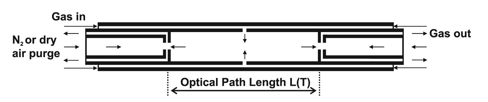
Figure 1: Schematic of the gas flow patterns in the high temperature ceramic gas cell (c-HGC) used in the measurements. The optical path length is defined by flow windows formed by counterwise gas flows (N₂ and gas of interest). See [34] for more details. Black arrows indicate flow direction. Reproduced from Ref. [35].

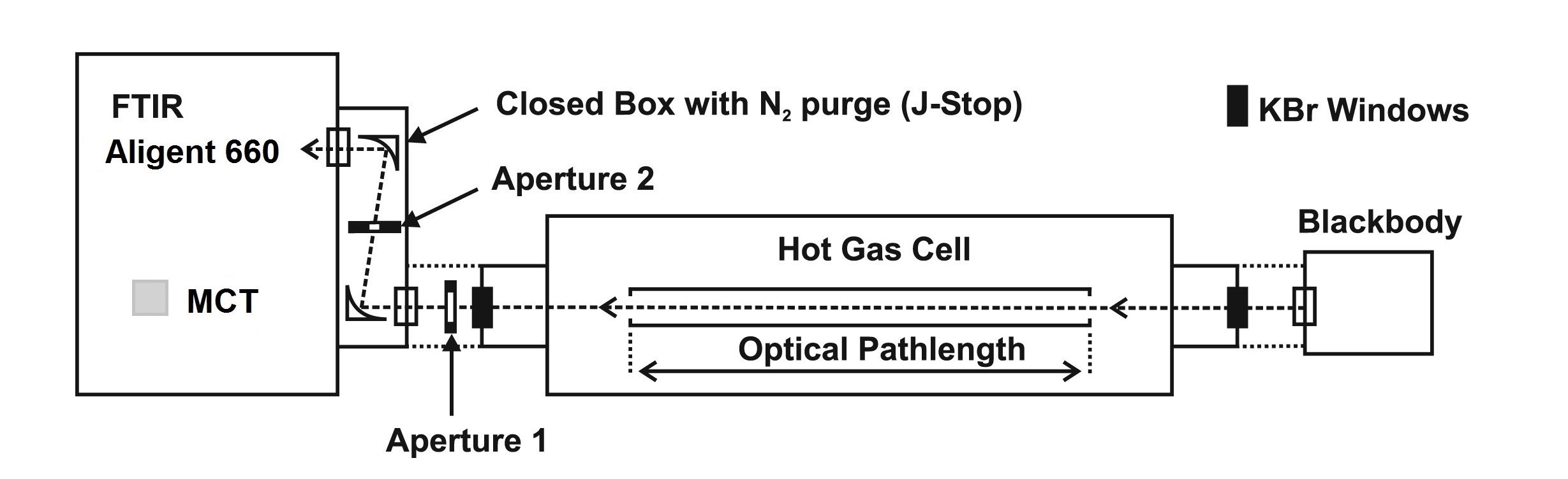
Figure 2: Experimental optical set up for NH₃ high-resolution measurements in the c-HGC. . Adapted from Ref. [35].

3 Data Analysis

This study used the BYTe [22] variational line list and experimental energies determined using the MARVEL procedure [17].

3.1 Calculating Experimental Absorption Spectra

Experimental transmission spectra $\tau_{\rm exp}(\nu,T)$ at a temperature $T$ [K] and a line position $\nu$ [cm^-1] are calculated from four SB spectra. This four measurements scheme is needed because the IR light source used is not modulated but modulation of the IR light appears in the FTIR spectrometer. Therefore, the MCT detector in the FTIR spectrometer will ”see” both modulated emissions from the light source and the cell. Moreover at 1027 ^∘C many of NH₃ bands appear in emission as well and the additional measurements with the cold beam stopper allow one to separate emission from absorption. The four measurements are two reference (N₂ in the central part of the cell) measurements $\mathbf{I}_{\rm ref+BB}$ and $\mathbf{I}_{\rm ref}$ and two sample (N₂ + NH₃ mixture) measurements $\mathbf{I}_{\rm gas+BB}$ and $\mathbf{I}_{\rm gas}$, one with and one without signal from the BB (at 1800 K) [13, 33]:

$$\tau_{\rm exp}(\nu,T)=\frac{\mathbf{I}_{\rm gas+BB}-\mathbf{I}_{\rm gas}}{\mathbf{I}_{\rm ref+BB}-\mathbf{I}_{\rm ref}}$$ (1)

Spectra without signal from the BB are measured from a cold (room temperature) beam stopper placed at 90 degrees from the optical axis of the setup using a movable mirror in the BB adapter. The absorption spectra are then calculated from the reference, $a_{0}$ ($=\mathbf{I}_{\rm ref+BB}-\mathbf{I}_{\rm ref}$), and sample, $a_{1}$ ($=\mathbf{I}_{\rm gas+BB}-\mathbf{I}_{\rm gas}$), measurements:

$$A_{\rm exp}(\nu,T)=\log_{10}\left[\frac{a_{0}}{a_{1}}\right]$$ (2)

3.2 Calculating Theoretical Absorption Spectra

The method for calculating theoretical absorption spectra follows Ref. [13]. First the ’true’ transmission spectrum was computed as:

$$\tau^{\rm true}_{\rm calc}(\nu,T)=\exp\left(-\sigma(\nu,T)lc\right)$$ (3)

where $l$ is the absorption path length in cm, $c$ is the NH₃ concentration in cm^-3 and $\sigma(\nu,T)$ is the pressure-broadened NH₃ absorption cross-section calculated using BYTe and the procedure laid out in [38], but replacing the Gaussian line shape with a Voigt line shape. Lorentz half-widths were estimated from the experimental spectra and with reference to measured widths compiled in the HITRAN database. The measured (effective) transmittance spectrum is derived by convolving $\tau^{\rm true}_{\rm calc}(\nu,T)$ with the instrument line shape (ILS) function $\Gamma(\nu-\nu_{0})$:

$$\tau^{\rm eff}_{\rm calc}(\nu,T)=\int_{0}^{\infty}\tau^{\rm true}_{\rm calc}(\nu_{0},T)\Gamma(\nu-\nu_{0})d\nu_{0}$$ (4)

For boxcar apodization, the ILS is a sinc function:

$$\Gamma(\nu)=\Lambda~{}{\rm sinc}(\Lambda\pi\nu)=\Lambda\frac{\sin(\Lambda\pi\nu)}{(\Lambda\pi\nu)}$$ (5)

For triangular apodization, the ILS is a $\textrm{sinc}^{2}$ function:

$$\Gamma(\nu)=\Lambda~{}{\rm sinc}^{2}(\Lambda\pi\nu)=2\Lambda\frac{\sin^{2}(\Lambda\pi\nu)}{(\Lambda\pi\nu)^{2}}$$ (6)

where $\Lambda$ is commonly termed the FTIR retardation and is generally defined as the inverse of the nominal resolution of the spectrometer [37].

The theoretical absorption spectrum is then computed as:

$$A_{\rm calc}(\nu,T)=\log_{10}\left[\frac{1}{\mathbf{\tau}^{\rm eff}_{\rm calc}(\nu,T)}\right]$$ (7)

3.3 The Assignment Procedure

First a list of observable BYTe lines for the experimental conditions was compiled. For this purpose the absorbance of each line, $j$, was approximated as:

$$A^{\rm approx}_{\rm calc}=\frac{S_{j}^{a}lc}{\Delta L\ln(10)}$$ (8)

where $\Delta L$ is an effective line width which is assumed to be a constant for all lines in the spectrum and the quantity $\frac{S_{j}^{a}}{\Delta L}$ represents an effective cross section assuming rectangular line shapes with $\Delta L$ widths.

If both the upper and lower energies involved in a observable transition were known experimentally, the BYTe line position was replaced by the MARVEL line position generated by subtracting upper and lower state energies. This hybrid line list, which retains all the BYTe transitions, will be presented elsewhere [39]; it shall henceforth be referred to as BARVEL.

Taking the resolution of the measurements and the accuracy of BYTe intensities into account (see Section 4.1), experimental peaks and BARVEL line positions were coupled using python scripts to produce a ’trivial’ assignment list. In cases where multiple BARVEL lines corresponded to a single peak, the peak was assigned to the strongest line.

Trivial assignments for the same vibrational band provide an expected observed minus calculated (obs. - calc.) difference for all lines in that band. Lines present in the list of observable BYTe lines, but not in BARVEL, were shifted by this residual to make future assignments by the method of branches [40].

A list of all trivial and branch assignments, the final assignment list, was then compared to previous studies, namely those catalogued in the HITRAN database [41].

4 Results and Discussion

The absorption measurements were performed at a temperature of 1027 ^∘C for the NH₃ volume concentration of 10$\%$.

The measurements were used to test the accuracy of BYTe then analysed using BYTe to generate an assignment list for the data. Central wavenumbers for assigned peaks are compared to line positions measured by Hargreaves et al. [11] where possible.

The absorption spectra, a peak list (partially assigned) including line positions from Hargreaves et al. [11] for assigned lines where available, and new energy level information derived from the assignments are presented in the supplementary data.

4.1 Direct Comparison with BYTe

A comparison between the experimental and theoretical absorption spectra at 1027 ^∘C for the whole region (2100 - 5500 cm^-1) is shown in Figure 3. Overall, taking into account the experimental noise, there is good agreement. However there are shifts in line position of the order $\pm$ 0.2 cm^-1 across the entire spectral range and shifts up to $\pm$ 1 - 2 cm^-1 in a few regions, particularly at higher wavenumbers. Hence it was decided that assignments should only be made using MARVEL line positions or BYTe line positions corrected for the expected obs. - calc. difference derived from trivial assignments, and not by simple line list comparison. BARVEL line positions should have an obs. - calc. difference smaller than the nominal resolution of the measurements, 0.09 cm^-1, whilst the wavenumber threshold for the BYTe line positions was taken to within 0.1 cm^-1 of the expected obs. - calc. difference. On the whole experimental line intensities are reproduced within 30 %. This is illustrated in Figure 4 for the region 4860 - 4900 cm^-1. As such experimental lines were coupled to BARVEL or BYTe lines using an intensity threshold of 30 %.

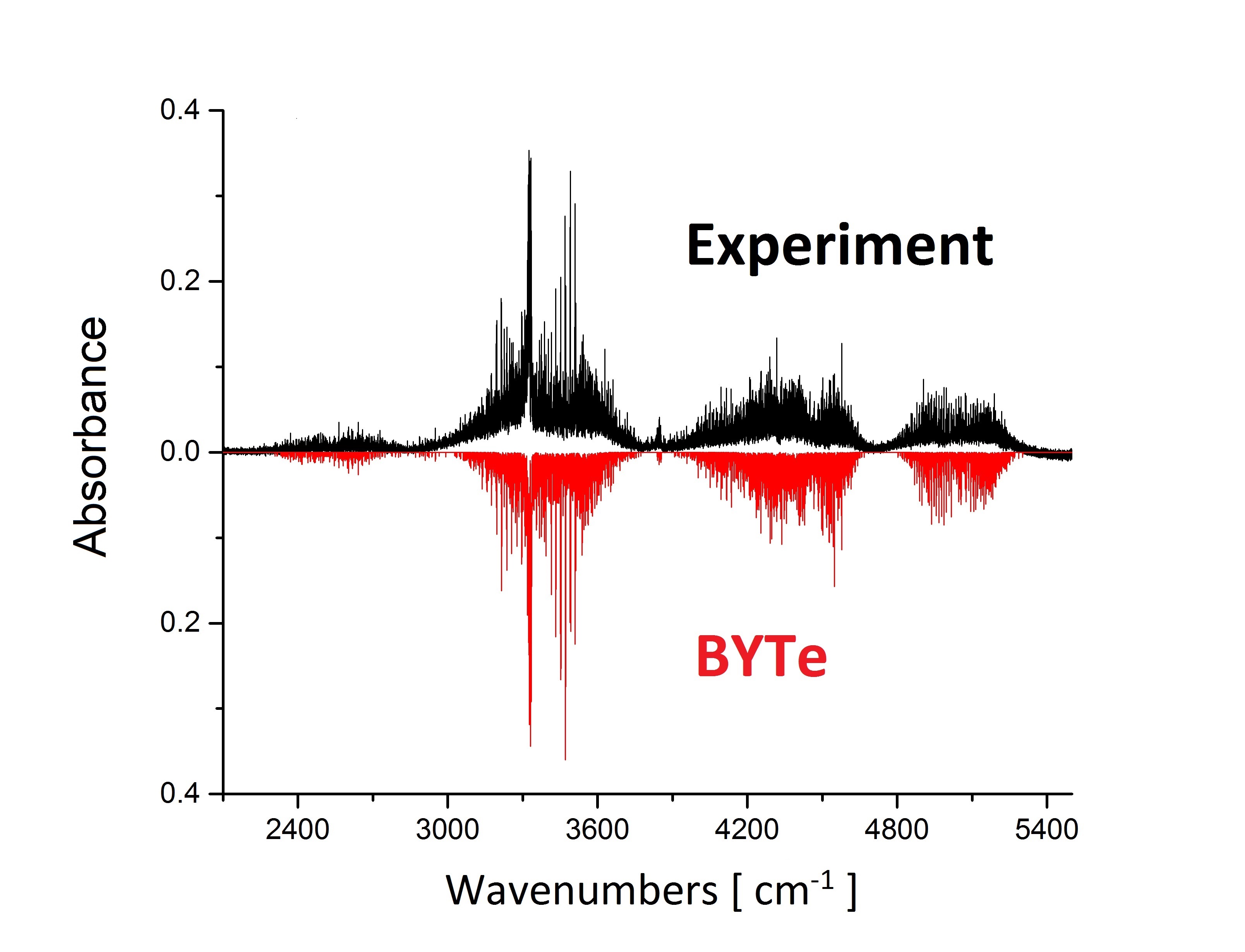
Figure 3: Comparison between experimental (upper) and calculated (BYTe, lower) absorption spectra at 1027 ^∘C for the range 2100 - 5500 cm^-1.

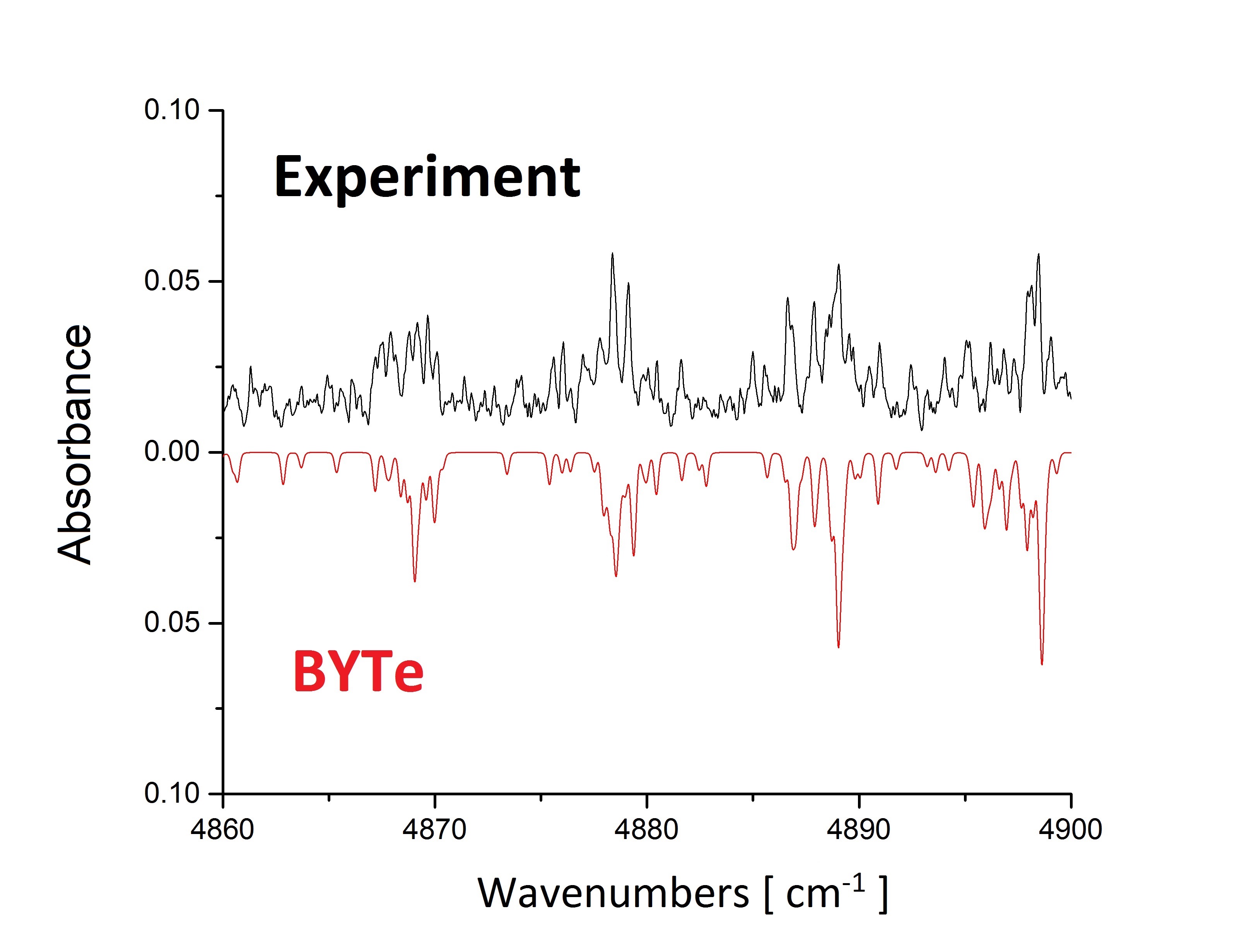
Figure 4: Comparison between experimental (upper) and calculated (BYTe, lower) absorption spectra at 1027 ^∘C for the range 4860 - 4900 cm^-1.

4.2 Assignments

Out of 3701 measured experimental peaks 2308 lines have been assigned. The remaining peaks either did not correspond to a BARVEL or BYTe line within the set wavenumber and intensity thresholds or corresponded to multiple lines with roughly equal contribution to the total intensity such that it could not be confidently assigned. 553 lines were previously assigned by studies included in the HITRAN database (see Table 1). The full 1027 ^∘C peak list with assignments is available as supplementary material to this article.

Hargreaves et al. [11] presented high temperature line lists for the region 2100 - 4000 cm^-1 constructed from emission spectra recorded at a resolution of 0.01 cm^-1. These line lists are currently being updated and extended (private communication) and hence were not the focus of the current work. Of the 1755 newly assigned lines in this work, 990 are also present in the line lists of Ref. [11]. In these cases line positions from Ref. [11] are included with the current central peak wavenumbers in the supplementary data and employed in the computation of upper state energies described below, as these were measured at a higher resolution.

For branch assignments with an experimentally known lower energy state, energies for the upper state were computed using MARVEL energies and the line position of the strongest assigned transition to that state. The calculated energies are available as supplementary material to this article.

Table 1: Summary of NH₃ lines assigned in the region 2100 - 5500 cm^-1.

	Lines
Experimental	3701
HITRAN	553
New trivial	272
New branch	1483
Total Assigned	2308

As in our previous study [13], lines were assigned to a large number of different bands. Table LABEL:t:bands gives a summary of the observed bands including the number of lines assigned to each and whether the band was observed for the first time in this work. Bands are listed in order of theoretical vibrational band centre (VBC). VBC = VBO^′- VBO^′′ where VBO is the vibrational band origin from BYTe, in wavenumbers. For simplicity abbreviated vibrational labels ($v_{1}v_{2}v_{3}^{L_{3}}v_{4}^{L_{4}}i$) [42] are used to identify bands in this table and only the highest value of the rotational quantum number $J$, assigned in this work for each band, is indicated. If the observed $J_{\mathrm{max}}$ in this work is bigger that quoted in the literature, the previous $J_{\mathrm{max}}$ is also given. The full 26 quantum labels for each transition, 13 per vibration-rotation state as recommended by Down et al. [42], will be given in the partially assigned peak list and energies files.

Table 2: Summary of observed bands in the region 2100 - 5500 cm^-1 in order of theoretical (BYTe) vibrational band centre (VBC = VBO^′ - VBO^′′ where VBO = vibrational band origin, in cm^-1) with maximum upper and lower $J$ rotational quantum number ($J^{\prime}_{\mathrm{max}}$ and $J^{\prime\prime}_{\mathrm{max}}$ respectively). $N$ is the number of lines assigned to the band. If $J_{\mathrm{max}}$ in this work is higher than given in the literature, the previously known $J_{\mathrm{max}}$ is given in parentheses. o$-$c gives the band shift used, in cm^-1, in making branch assignments. VBO of $0^{+}$ is set to 0.0 cm^-1 in line with the MARVEL study [17].

Band	VBC	$N$	$J^{\prime}_{\mathrm{max}}$	$J^{\prime\prime}_{\mathrm{max}}$	o$-$c	Note
$\nu_{3}^{1,-}-\nu_{2}^{-}$	2475.50	59	17 (12)	16	$-$0.1
$\nu_{3}^{1,+}-\nu_{2}^{+}$	2511.55	52	19 (12)	18	0.1
$(\nu_{2}+\nu_{3}^{1})^{-}-2\nu_{2}^{-}$	2553.27	14	16 (11)	15	0.1	New
$(\nu_{2}+\nu_{3}^{1})^{+}-2\nu_{2}^{+}$	2553.27	6	9	9	0.1	New
$3\nu_{2}^{-}-0^{+}$	2895.53	6	9	9	0.1
$(\nu_{1}+2\nu_{2})^{+}-2\nu_{2}^{-}$	3120.69	8	16 (11)	16	$-$2.0
$(\nu_{2}+2\nu_{4}^{0})^{+}-\nu_{2}^{+}$	3147.49	1	8	8	$-$0.6	New
$(\nu_{2}+2\nu_{4}^{2})^{+}-\nu_{2}^{+}$	3167.81	19	18 (7)	19	0.0	New
$(2\nu_{2}+\nu_{4}^{1})^{+}-0^{+}$	3189.04	17	15 (11)	14	1.0
$2\nu_{4}^{0,+}-0^{-}$	3215.21	95	21 (12)	20	0.3
$2\nu_{4}^{0,+}-0^{+}$	3216.00	2	6	7	0.3
$2\nu_{4}^{0,-}-0^{-}$	3216.75	13	17 (12)	18	$-$0.2
$2\nu_{4}^{0,-}-0^{+}$	3217.55	72	18 (12)	17	0.4
$2\nu_{4}^{2,+}-0^{-}$	3239.39	5	9	8	$-$0.1
$2\nu_{4}^{2,+}-0^{+}$	3240.18	82	24 (13)	25	$-$0.2
$2\nu_{4}^{2,-}-0^{-}$	3240.78	53	21 (13)	22	$-$0.2
$(\nu_{2}+2\nu_{4}^{0})^{-}-\nu_{2}^{-}$	3240.81	1	7	8	0.0	New
$2\nu_{4}^{2,-}-0^{+}$	3241.58	23	17 (13)	18	0.1
$(\nu_{2}+2\nu_{4}^{2})^{-}-\nu_{2}^{-}$	3260.70	8	16 (8)	17	0.0	New
$2\nu_{1}^{+}-2\nu_{4}^{0,-}$	3296.58	1	4	4	1.0	New
$(\nu_{1}+\nu_{2})^{+}-\nu_{2}^{-}$	3326.39	62	22 (11)	22	0.05
$(\nu_{1}+\nu_{4}^{1})^{+}-\nu_{4}^{1,-}$	3328.35	19	14 (13)	15	0.0	New
$(\nu_{1}+\nu_{4}^{1})^{-}-\nu_{4}^{1,-}$	3329.51	11	15 (12)	16	0.0	New
$(\nu_{1}+\nu_{4}^{1})^{-}-\nu_{4}^{1,+}$	3330.61	10	13 (12)	14	0.0	New
$\nu_{1}^{+}-0^{-}$	3335.28	158	21 (12)	21	$-$0.4
$\nu_{1}^{-}-0^{+}$	3337.07	155	21 (12)	21	$-$0.4
$(\nu_{1}+\nu_{2})^{-}-\nu_{2}^{+}$	3387.59	85	19 (12)	19	$-$0.05
$\nu_{3}^{1,-}-0^{-}$	3443.20	142	22 (12)	22	0.1
$(\nu_{3}^{1}+\nu_{4}^{1})^{+}-\nu_{4}^{1,+}$	3443.60	2	6	7	0.1	New
$\nu_{3}^{1,+}-0^{+}$	3443.62	160	23 (12)	24	0.1
$(\nu_{2}+\nu_{3}^{1})^{+}-\nu_{2}^{+}$	3448.80	110	19 (12)	20	0.2
$(\nu_{2}+\nu_{3}^{1})^{-}-\nu_{2}^{+}$	3467.32	1	7	7	0.2
$(\nu_{2}+\nu_{3}^{1})^{-}-\nu_{2}^{-}$	3503.01	73	19 (11)	20	0.2
$(2\nu_{2}+\nu_{3}^{1})^{-}-2\nu_{2}^{-}$	3470.63	18	14 (7)	15	0.3	New
$(2\nu_{2}+\nu_{3}^{1})^{+}-2\nu_{2}^{+}$	3548.80	74	21 (11)	22	0.0	New
$(2\nu_{2}+\nu_{3}^{1})^{+}-\nu_{2}^{+}$	4178.16	89	18 (11)	17	$-$0.6	New
$(\nu_{1}+\nu_{2})^{+}-0^{-}$	4293.73	11	12 (11)	12	0.05
$(\nu_{1}+\nu_{2})^{-}-0^{+}$	4320.03	12	13 (12)	12	0.0
$(\nu_{2}+\nu_{3}^{1})^{+}-0^{+}$	4416.93	123	19 (12)	18	0.2
$(2\nu_{2}+\nu_{3}^{1})^{-}-\nu_{2}^{-}$	4420.38	93	16 (7)	17	0.4	New
$(\nu_{2}+\nu_{3}^{1})^{+}-0^{-}$	4434.66	129	19 (11)	18	0.2
$(\nu_{1}+\nu_{4}^{1})^{+}-0^{+}$	4955.73	100	18 (13)	18	0.0
$(\nu_{1}+\nu_{4}^{1})^{-}-0^{-}$	4956.10	130	19 (12)	20	$-$0.1
$(\nu_{3}^{1}+\nu_{4}^{1})^{-}-0^{-}$	5069.59	3	9 (8)	9	$-$1.0
$(\nu_{3}^{1}+\nu_{4}^{1})^{+}-0^{+}$	5069.88	1	8	9	0.4

15 bands have been assigned for the first time in this work, although some of the energy levels involved are known from observations of other bands.

All trivial assignments are secure, as the MARVEL energies (and hence BARVEL line positions) are known to very high accuracy (of the order 10^-4 cm^-1 for the energies). The accuracy of branch assignments depends on the determination of the obs. - calc. difference for a given vibrational band.

For bands with many ($>$ 10) assignments the obs. - calc. difference can be tracked through the band. As this remains relatively stable we have confidence in our assignments.

Bands for which only a few lines could be assigned are more tentative, although every observed band in this work has at least one associated trivial assignment.

It is worth noting that the single lines assigned to $(\nu_{2}+2\nu_{4}^{0})^{+}-\nu_{2}^{+}$, $(\nu_{2}+2\nu_{4}^{0})^{-}-\nu_{2}^{-}$, $2\nu_{1}^{+}-2\nu_{4}^{0,-}$, $(\nu_{2}+\nu_{3}^{1})^{-}-\nu_{2}^{+}$ and $(\nu_{3}^{1}+\nu_{4}^{1})^{+}-0^{+}$ are all trivial.

5 Summary

High-resolution absorption measurements of NH₃ in the region 2100 - 5500 cm^-1 at atmospheric pressure and a temperature of 1027 ^∘C have been reported and analysed.

A comparison between the measurements and BYTe shows in general good agreement through there are some shifts in line position (up to 2 cm^-1) and overall BYTe reproduces experimental intensities only within 30 %. Work towards a new NH₃ line list is currently being carried out as part of the ExoMol project [27].

The use of BYTe and MARVEL has allowed the assignment of 2308 lines. 553 lines were previously assigned by studies included in the HITRAN database. 1755 lines have been assigned for the first time in this work. The 272 lines assigned using MARVEL line positions, also known as trivial assignments, are secure as the accuracy of MARVEL energies is of the order 10^-4 cm^-1. Of the 1483 branch assignments, those associated with bands which have numerous assignments in this work should be reliable because the observed-calculated differences remain relatively stable within a given band. The remaining assignments should also be valid, as all observed bands have at least one verified assignment in this work which provides an expected observed-calculated difference for the band, however these are more tentative.

References

- [1] D. C. Trimble, AIR QUALITY: Information on Tall Smokestacks and Their Contribution to Interstate Transport of Air Pollution, Tech. rep., GAO U.S. Government Accountability Office, published: May 11. Publicly Released: Jun 10 (2011).
- [2] A. Fateev, S. Clausen, High-resolution spectroscopy of gases at elevated temperatures for industrial applications, in: 22nd UCL Astrophysics Colloquium: Opacities in Cool Stars and Exoplanets, 2012.
- [3] M. R. Schmidt, J. H. He, R. Szczerba, V. Bujarrabal, J. Alcolea, J. Cernicharo, L. Decin, K. Justtanont, D. Teyssier, K. M. Menten, D. A. Neufeld, H. Olofsson, P. Planesas, A. P. Marston, A. M. Sobolev, A. de Koter, F. M. Schöier, Herschel/HIFI observations of the circumstellar ammonia lines in IRC+10216, Astron. Astrophys.Accepted.
- [4] D. A. Ladeyschikov, M. S. Kirsanova, A. P. Tsivilev, A. M. Sobolev, Molecular emission in dense massive clumps from the star-forming regions S231–S235, Astrophysical Bulletin 71 (2016) 208–224.
- [5] J. Harju, F. Daniel, O. Sipila, P. Caselli, J. E. Pineda, R. K. Friesen, A. P. R. Güsten, L. Wiesenfeld, P. C. Myers, A. Faure, P. Hily-Blant, C. Rist, E. Rosolowsky, S. Schlemmer, Y. L. Shirley, Deuteration of ammonia in the starless core Ophiuchus/H-MM1, Astron. Astrophys.Submitted.
- [6] J. I. Canty, P. W. Lucas, J. Tennyson, S. N. Yurchenko, S. K. Leggett, C. G. Tinney, H. R. A. Jones, B. Burningham, D. J. Pinfield, R. L. Smart, Methane and Ammonia in the near-infrared spectra of late T dwarfs, Mon. Not. R. Astron. Soc. 450 (2015) 454–480. doi:10.1093/mnras/stv586.
- [7] S. K. Leggett, C. V. Morley, M. S. Marley, D. Saumon, NEAR-INFRARED PHOTOMETRY OF Y DWARFS: LOW AMMONIA ABUNDANCE AND THE ONSET OF WATER CLOUDS, Astrophys. J. 799 (2015) 37. doi:{10.1088/0004-637X/799/1/37}.
- [8] J. H. Woodman, L. Trafton, T. Owen, The abundances of ammonia in the atmospheres of Jupiter, Saturn, AND Titan, Icarus 32 (1977) 314–320.
- [9] V. N. Salinas, M. R. Hogerheijde, E. A. Bergin, L. Ilsedore Cleeves, C. Brinch, G. A. Blake, D. C. Lis, G. J. Melnick, O. Panic, J. C. Pearson, L. Kristensen, U. A. Yildiz, E. F. van Dishoeck, First detection of gas-phase ammonia in a planet-forming disk, Astron. Astrophys. 591 (2016) A122.
- [10] R. J. Hargreaves, G. Li, P. F. Bernath, Ammonia line lists from 1650 to 4000 cm-1, J. Quant. Spectrosc. Radiat. Transf. 113 (2012) 670–679.
- [11] R. J. Hargreaves, G. Li, P. F. Bernath, Hot NH3 spectra for astrophysical applications, Astrophys. J. 735 (2012) 111.
- [12] N. F. Zobov, S. V. Shirin, R. I. Ovsyannikov, O. L. Polyansky, S. N. Yurchenko, R. J. Barber, J. Tennyson, R. Hargreaves, P. Bernath, Analysis of high temperature Ammonia spectra from 780 to 2100 cm-1, J. Mol. Spectrosc. 269 (2011) 104–108.
- [13] E. J. Barton, S. N. Yurchenko, J. Tennyson, S. Clausen, A. Fateev, High-resolution absorption measurements of NH3 at high temperatures: 500 - 2100 cm-1, J. Quant. Spectrosc. Radiat. Transf. 167 (2015) 126–134. doi:10.1016/j.jqsrt.2015.07.020.
- [14] E. J. Barton, S. N. Yurchenko, J. Tennyson, S. Béguier, A. Campargue, A near infrared line list for NH3: Analysis of a Kitt Peak spectrum after 35 years, J. Mol. Spectrosc. 325 (2016) 7–12. doi:10.1016/j.jms.2016.05.001.
- [15] P. Cermák, J. Hovorka, P. Veis, P. Cacciani, J. Cosléou, J. E. Romh, M. Khelkhal, Spectroscopy of 14nh3 and 15nh3 in the 2.3 m spectral range with a new vecsel laser source, J. Quant. Spectrosc. Radiat. Transfer 137 (2014) 13–22.
- [16] P. Cacciani, P. Cermák, J. Cosléou, J. El Rohm, J. Hovorka, M. Khelkhal, Spectroscopy of ammonia in the range 6626–6805 cm-1: using temperature dependence towards a complete list of lower state energy transitions, Mol. Phys. 112 (2014) 2476–2485.
- [17] A. R. Al Derzi, T. Furtenbacher, S. N. Yurchenko, J. Tennyson, A. G. Császár, MARVEL analysis of the measured high-resolution spectra of 14NH3, J. Quant. Spectrosc. Radiat. Transf. 161 (2015) 117–130. doi:10.1016/j.jqsrt.2015.03.034.
- [18] T. Furtenbacher, A. G. Császár, J. Tennyson, MARVEL: measured active rotational-vibrational energy levels, J. Mol. Spectrosc. 245 (2007) 115–125.
- [19] T. Furtenbacher, A. G. Császár, MARVEL: measured active rotational-vibrational energy levels. II. Algorithmic improvements, J. Quant. Spectrosc. Radiat. Transf. 113 (2012) 929–935.
- [20] K. Sung, S. Yu, J. Pearson, O. Pirali, F. K. Tchana, L. Manceron, Far-infrared 14nh3 line positions and intensities measured with a ft-ir and {AILES} beamline, synchrotron {SOLEIL}, J. Mol. Spectrosc. 327 (2016) 1–20. doi:http://dx.doi.org/10.1016/j.jms.2016.06.011.
- [21] S. N. Yurchenko, R. J. Barber, A. Yachmenev, W. Thiel, P. Jensen, J. Tennyson, A variationally computed =300 K line list for NH3, J. Phys. Chem. A 113 (2009) 11845–11855.
- [22] S. N. Yurchenko, R. J. Barber, J. Tennyson, A variationally computed hot line list for NH3, Mon. Not. R. Astron. Soc. 413 (2011) 1828–1834.
- [23] X. Huang, D. W. Schwenke, T. J. Lee, Rovibrational spectra of ammonia. II. Detailed analysis, comparison, and prediction of spectroscopic assignments for 14NH3, 15NH3, and 14ND3, J. Chem. Phys. 134 (2011) 044321. doi:10.1063/1.3541352.
- [24] E. J. Barton, O. L. Polyansky, S. N. Yurchenko, J. Tennyson, S. Civis, M. Ferus, R. H. a. O. . F. Bernath, A. Kyuberis, N. F. Zobov, S. Béguier, A. Campargue, Absorption spectra of ammonia near 1 m, J. Mol. Spectrosc.
- [25] S. N. Yurchenko, R. J. Barber, J. Tennyson, W. Thiel, P. Jensen, Towards efficient refinement of molecular potential energy surfaces: Ammonia as a case study, J. Mol. Spectrosc. 268 (2011) 123–129.
- [26] S. N. Yurchenko, W. Thiel, P. Jensen, Theoretical ROVibrational Energies (TROVE): A robust numerical approach to the calculation of rovibrational energies for polyatomic molecules, J. Mol. Spectrosc. 245 (2007) 126–140. doi:10.1016/j.jms.2007.07.009.
- [27] J. Tennyson, S. N. Yurchenko, ExoMol: molecular line lists for exoplanet and other atmospheres, Mon. Not. R. Astron. Soc. 425 (2012) 21–33.
- [28] J. Tennyson, S. N. Yurchenko, A. F. Al-Refaie, E. J. Barton, K. L. Chubb, P. A. Coles, S. Diamantopoulou, M. N. Gorman, C. Hill, A. Z. Lam, L. Lodi, L. K. McKemmish, Y. Na, A. Owens, O. L. Polyansky, T. Rivlin, C. Sousa-Silva, D. S. Underwood, A. Yachmenev, E. Zak, The ExoMol database: molecular line lists for exoplanet and other hot atmospheres, J. Mol. Spectrosc. 327 (2016) 73–94. doi:10.1016/j.jms.2016.05.002.
- [29] X. Huang, D. W. Schwenke, T. J. Lee, Rovibrational spectra of ammonia. i. unprecedented accuracy of a potential energy surface used with nonadiabatic corrections, J. Chem. Phys. 134 (2011) 044320.
- [30] X. Huang, D. W. Schwenke, T. J. Lee, Rovibrational spectra of ammonia. II. Detailed analysis, comparison, and prediction of spectroscopic assignments for 14NH3, 15NH3, and 14ND3, J. Chem. Phys. 134 (2011) 044321.
- [31] K. Sung, L. R. Brown, X. Huang, D. W. Schwenke, T. J. Lee, S. L. Coy, K. K. Lehmann, Extended line positions, intensities, empirical lower state energies and quantum assignments of nh3 from 6300 to 7000 cm-−1, J. Quant. Spectrosc. Radiat. Transfer 113 (2012) 1066–1083. doi:10.1016/j.jqsrt.2012.02.037.
- [32] S. Clausen, K. A. Nielsen, A. Fateev, Ceramic gas cell operating up to 1873 K, Measurement Science and TechnologyIn preparation.
- [33] V. Evseev, A. Fateev, S. Clausen, High-resolution transmission measurements of CO2 at high temperatures for industrial applications, J. Quant. Spectrosc. Radiat. Transf. 113 (2012) 2222–2233.
- [34] V. Bercher, S. Clausen, A. Fateev, H. Spliethoff, Oxyfuel combustion, International Greenhouse Gas control 5 (2011) S76–99.
- [35] M. Alberti, R. Weber, M. Mancini, A. Fateev, S. Clausen, Validation of HITEMP-2010 for carbon dioxide and water vapour at high temperatures and atmospheric pressure in 450-7600 spectral range, J. Quant. Spectrosc. Radiat. Transf. 157 (2015) 14–33.
- [36] A. Fateev, S. Clausen, Online non-contact gas analysis, Tech. rep., Technical University of Denmark, contract no.: Energinet.dk no. 2006 1 6382. (2008).
- [37] P. R. Griffiths, J. A. de Haseth, Fourier transform infrared spectroscopy, 2nd Edition, Wiley, Chichester, UK, 2007.
- [38] C. Hill, S. N. Yurchenko, J. Tennyson, Temperature-dependent molecular absorption cross sections for exoplanets and other atmospheres, Icarus 226 (2013) 1673–1677.
- [39] C. A. Beale, R. J. Hargreaves, P. A. Coles, J. Tennyson, P. F. Bernath, Infrared absorption spectra of hot ammonia, J. Quant. Spectrosc. Radiat. Transf.
- [40] O. L. Polyansky, N. F. Zobov, S. Viti, J. Tennyson, P. F. Bernath, L. Wallace, K band spectrum of water in sunspots, Astrophys. J. 489 (1997) L205–L208.
- [41] L. S. Rothman, I. E. Gordon, Y. Babikov, A. Barbe, D. C. Benner, P. F. Bernath, M. Birk, L. Bizzocchi, V. Boudon, L. R. Brown, A. Campargue, K. Chance, E. A. Cohen, L. H. Coudert, V. M. Devi, B. J. Drouin, A. Fayt, J.-M. Flaud, R. R. Gamache, J. J. Harrison, J.-M. Hartmann, C. Hill, J. T. Hodges, D. Jacquemart, A. Jolly, J. Lamouroux, R. J. Le Roy, G. Li, D. A. Long, O. M. Lyulin, C. J. Mackie, S. T. Massie, S. Mikhailenko, H. S. P. Müller, O. V. Naumenko, A. V. Nikitin, J. Orphal, V. Perevalov, A. Perrin, E. R. Polovtseva, C. Richard, M. A. H. Smith, E. Starikova, K. Sung, S. Tashkun, J. Tennyson, G. C. Toon, V. G. Tyuterev, G. Wagner, The HITRAN 2012 molecular spectroscopic database, J. Quant. Spectrosc. Radiat. Transf. 130 (2013) 4 – 50. doi:10.1016/jqsrt.2013.07.002.
- [42] M. J. Down, C. Hill, S. N. Yurchenko, J. Tennyson, L. R. Brown, I. Kleiner, Re-analysis of ammonia spectra: Updating the HITRAN 14NH3 database, J. Quant. Spectrosc. Radiat. Transf. 130 (2013) 260–272.