The Minimal Geometric Deformation Approach:
a brief introduction

Abstract

We review the basic elements of the Minimal Geometric Deformation approach in details. This method has been successfully used to generate brane-world configurations from general relativistic perfect fluid solutions.

1 Introduction

General Relativity (GR) represents one of the pillars of modern Physics. The predictions made by this theory range from the perihelion shift of Mercury, the deflexion of light and gravitational lensing, the gravitational redshift and time delay, and the existence of black holes. The observation of these effects, as well as the recent detection of the gravitational waves GW150914 [1] and GW151226 [2], have given GR the status of the benchmark theory of the gravitational interaction (for an excellent review, see Ref. [3] and references therein). Why do we want to find new gravitational theories beyond GR then? The reason has to do with some fundamental questions associated with the gravitational interaction which GR does not seem to be able to answer satisfactorily. One is the problem of dark matter and dark energy, which require introducing some unknown matter-energy to reconcile GR predictions with the observations of galactic rotation curves and accelerated expansion of the universe, respectively. Then, there is the difficulty of reconciling GR with the Standard Model of particle physics, or equivalently, the failure to quantise GR by the same successful scheme used with the other fundamental interactions. Such issues have motivated the search of a new gravitational theory beyond GR that could help to explain part of the problems mentioned above. Indeed, there is already a long list of alternative theories, like $f(R)$ and higher curvature theories, Galileon theories, scalar-tensor theories, (new and topological) massive gravity, Chern-Simons theories, higher spin gravity theories, Horava-Lifshitz gravity, extra-dimensional theories, torsion theories, Horndeski’s theory, etc (See for instance Refs. [4]–[17]). Nonetheless, quantum gravity is still an open problem, and dark matter and dark energy remain a mystery so far.

The MGD was originally proposed [18] in the context of the the Randall-Sundrum brane-world [19, 20] and extended to investigate new black hole solutions [21, 22]. While the brane-world is still an attractive scenario, since it explains the hierarchy of fundamental interactions in a simple way, to find interior solutions for self-gravitating systems is a difficult task, mainly due to the existence of non-linear terms in the matter fields. In addition, the effective four-dimensional Einstein equations are not a closed system, due to the extra-dimensional effects resulting in terms undetermined by the four-dimensional equations. Despite these complications, the MGD has proven to be useful, among other things, to derive exact and physically acceptable solutions for spherically symmetric and non-uniform stellar distributions [23, 26] as well; to express the tidal charge in the metric found in Ref. [27] in terms of the usual Arnowitt-Deser-Misner (ADM) mass [28]; to study microscopic black holes [29]; to clarify the role of exterior Weyl stresses acting on compact stellar distributions [30, 31]; to extend the concept of variable tension introduced in Refs. [32] by analysing the shape of the black string in the extra dimension [33]; to prove, contrary to previous claims, the consistency of a Schwarzschild exterior [34] for a spherically symmetric self-gravitating system made of regular matter in the brane-world; to derive bounds on extra-dimensional parameters [35] from the observational results of the classical tests of GR in the Solar system; to investigate the gravitational lensing phenomena beyond GR [36]; to determine the critical stability region for Bose-Einstein condensates in gravitational systems [37]; to study Dark $SU(N)$ glueball stars on fluid branes [38] as well as the correspondence between sound waves in a de Laval propelling nozzle and quasinormal modes emitted by brane-world black holes [39].

This brief review is organised as follows: the simplest ways to modified gravity are presented in Section 2, emphasising some problems that arise when the GR limit is considered; in Section 3, we recall the Einstein field equations on the brane for a spherically symmetric and static distribution of density $\rho$ and pressure $p$; in Section 4, the GR limit is discussed and the basic elements of the MGD are presented in section 5; in Section 6, we review the matching conditions between the interior and exterior space-time of self-gravitating systems within the MGD, and a recipe with the basic steps to implement the MGD is described in Section 7; finally, some conclusions are presented in the last section.

2 GR simplest extensions and their GR limit

This Section is devoted to describe in a qualitative way the so-called GR-limit problem, which arises when an extension to GR is considered. An explicit and quantitative description of this problem, as well as an explicit solution, is developed throughout the rest of the review.

One cannot try and change GR without considering the well-established and very useful Lovelock’s theorem [40], which severely restricts any possible ways of modifying GR in four dimensions. We will now show the simplest generic way.

Any extension to GR will eventually produce new terms in the effective four-dimensional Einstein equations. These “corrections” are usually handled as part of an effective energy-momentum tensor and appear in such a way that they should vanish or be negligible in an appropriate limit. For instance, they must vanish (or be negligible) at solar system scales, where GR has been successfully tested so far. This limit represents not only a critical point for a consistent extension of GR, but also a non-trivial problem that must be treated carefully.

The simplest way to extend GR is by considering a modified Einstein-Hilbert action,

$$S=\int\left[\frac{R}{2\,k^{2}}+{\cal L}\right]\sqrt{-g}\,d^{4}x+\alpha\,({\rm correction})\ ,$$ (2.1)

where $\alpha$ is a free parameter associated with the new gravitational sector not described by GR, as is schematically shown in Fig 1. The explicit form corresponding to the generic correction shown in Eq. (2.1) should be, of course, a well justified and physically motivated expression. At this stage the GR limit, obtained by setting $\alpha=0$, is just a trivial issue, so everything looks consistent. Indeed, we may go further and calculate the equations of motion from setting the variation $\delta S=0$ corresponding to this new theory,

$$R_{\mu\nu}-\frac{1}{2}\,R\,g_{\mu\nu}=k^{2}\,T_{\mu\nu}+\alpha\,({\rm new\ terms})_{\mu\nu}\ .$$ (2.2)

The new terms in Eq. (2.2) may be viewed as part of an effective energy-momentum tensor, whose explicit form may contain new fields, like scalar, vector and tensor fields, all of them coming from the new gravitational sector not described by Einstein’s theory. At this stage the GR limit, again, is a trivial issue, since $\alpha=0$ leads to the standard Einstein’s equations $G_{\mu\nu}=k^{2}\,T_{\mu\nu}$.

All the above seems to tell us that the consistency problem, namely the GR limit, is trivial. However, when the system of equations given by the expression (2.2) is solved, the result may show a complete different story. In general, and this is very common, the solution eventually found cannot reproduce the GR limit by simply setting $\alpha=0$. The cause of this problem is the non-linearity of Eq. (2.2), and should not be a surprise. To clarify this point, let us consider a spherically symmetric perfect fluid, for which GR uniquely determines the metric component

$$g^{-1}_{rr}=1-\frac{2\,m(r)}{r}\ ,$$ (2.3)

where $m$ is the mass function of the self-gravitating system. Now, let us consider the same perfect fluid in the “new” gravitational theory (2.1). When Eq. (2.2) is solved, we obtain an expression which generically may be written as

$$g^{-1}_{rr}=1-\frac{2\,m(r)}{r}+({\rm geometric\ deformation})\ ,$$ (2.4)

where by geometric deformation one should understand the deformation of the metric component (2.3) due to the generic extension (2.1) of GR. (“deformation” hence means a deviation from the GR solution). It is now very important to note that the deformation (2.4) always produces anysotropic consequences on the perfect fluid, namely, the radial and tangential pressures are no longer the same and in consequence the self-gravitating system will not be described as a perfect fluid anymore. Indeed, and this is a critical point in our analysis, the anisotropy produced by the geometric deformation always takes the form (See further Eqs. (5.7)-(5.11) to see an explicit calculation)

$${\cal P}=A+\alpha\,B\ .$$ (2.5)

This expression is very significant, since it shows that the GR limit cannot be a posteriori recovered by setting $\alpha=0$, since the “sector” denoted by $A$ in the anisotropy (2.5) does not depend on $\alpha$. Consequently, the perfect fluid GR solution ($A=0$) is not trivially contained in this extension, and one might say that we have an extension to GR which does not contain GR. This is of course a contradiction, or more properly a consistency problem, whose source can be precisely traced back to the geometric deformation shown in Eq. (2.4). The latter always takes the form (See Eq. (5.5) for an explicit expression)

$$({\rm geometric\ deformation})=X+\alpha\,Y\ ,$$ (2.6)

which contains a “sector” $X$ that does not depend on $\alpha$. This is again obviously inconsistent, since the deformation undergone by GR must depend smoothly on $\alpha$ and vanish with it. At the level of solutions, the source of this problem is the high non-linearity of the effective Einstein equations (2.2), which we want to emphasise has nothing to do with any specific extension of GR. Indeed, it is a characteristic of any high non-linear systems.

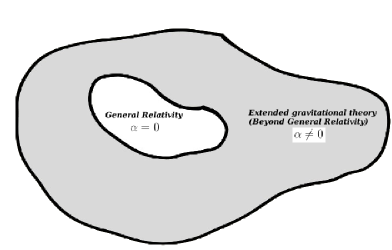
Figure 1: The new gravitational sector outside GR is parametrised by $\alpha$, so that GR represents a “sub-space” in the extended theory of gravity. When the free parameter $\alpha$ is turned off, we should automatically recover the domain of GR.

A method that solves the non-trivial issue of consistency with GR described above is the so-called Minimal Geometric Deformation MGD approach [18]. The idea is to keep under control the anisotropic consequences on GR appearing in the extended theory, in such a way that the $\alpha$-independent sector in the geometric deformation shown as $X$ in Eq. (2.6) always vanishes. Correspondingly, the $\alpha$-independent sector of the anisotropy $A$ in Eq. (2.5) will also vanish. This will ensure a consistent extension that recovers GR in the limit $\alpha\to 0$. In this approach, the generic expression $Y$ in Eq. (2.6) represents the minimal geometric deformation undergone by the radial metric component, the generic expression $B$ in Eq. (2.5) being the minimal anysotropic consequence undergone by GR due to correction terms in the modified Einstein-Hilbert action (2.1). The next key point is how we can make sure $X=0$ in Eq. (2.6) in order to obtain a consistent extension to GR. This is accomplished when a GR solution is forced to remian a solution in the extended theory. Roughly speaking, we need to introduce the GR solution into the new theory, as far as possible, as suggested in Fig 2. This provides the foundation for the MGD approach. We want to emphasise that the GR solution used to set $X=0$ in Eq. (2.6) will eventually be modified by using, for instance, the matching conditions at the surface of a self-gravitating system. One will therefore obtain physical variables that depend on the free parameter of the theory, here generically named $\alpha$. This free parameter could be, for instance, the one that measures deviation from GR in $f(R)$ theories, the brane tension in the brane-world, and so.

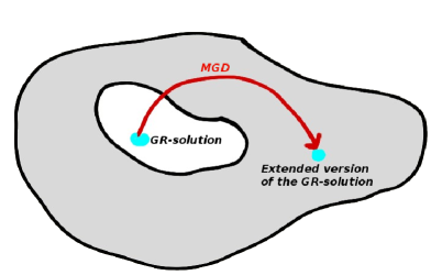
Figure 2: When a GR solution is forced to be a solution in the new gravitational sector by the MGD, the $\alpha$-independent terms in the extended solution are eliminated, and the GR limit is recovered.

3 Extra-dimensional gravity: the brane-world

In the generalised RS brane-world scenario, gravity lives in five dimensions and affects the gravitational dynamics in the (3+1)-dimensional universe accessible to all other physical fields, the so-called brane. The 5-dimensional Einstein equations projected on the brane give rise to the modified 4-dimensional Einstein equations [41, 42, 43] 

$$G_{\mu\nu}=-k^{2}\,T_{\mu\nu}^{\mathrm{eff}}-\Lambda\,g_{\mu\nu}\ ,$$ (3.1)

where $G_{\mu\nu}$ is the 4-dimensional Einstein tensor. The effective energy-momentum tensor is given by

$$T_{\mu\nu}^{\mathrm{eff}}=T_{\mu\nu}+\frac{6}{\sigma}\,S_{\mu\nu}+\frac{1}{8\,\pi}\,\mathcal{E}_{\mu\nu}+\frac{4}{\sigma}\,\mathcal{F}_{\mu\nu}\ ,$$ (3.2)

where $\sigma$ is the brane tension (which plays the role of the parameter $\alpha$ of the previous Section) and

$$T_{\mu\nu}=(\rho+p)\,u_{\mu}\,u_{\nu}-p\,g_{\mu\nu}$$ (3.3)

is the 4-dimensional energy-momentum tensor of brane matter described by a perfect fluid with 4-velocity field $u^{\mu}$, density $\rho$ and isotropic pressure $p$. The extra term

$$S_{\mu\nu}=\frac{T}{12}\,T_{\mu\nu}-\frac{1}{4}\,T_{\mu\alpha}\,T_{\ \nu}^{\alpha}+\frac{g_{\mu\nu}}{24}\left(3\,T_{\alpha\beta}\,T^{\alpha\beta}-T^{2}\right)$$ (3.4)

represents a local high-energy correction quadratic in $T_{\mu\nu}$ (with $T=T_{\alpha}^{\ \alpha}$), whereas

$$k^{2}\,\mathcal{E}_{\mu\nu}=\frac{6}{\sigma}\left[\mathcal{U}\left(u_{\mu}\,u_{\nu}+\frac{1}{3}\,h_{\mu\nu}\right)+\mathcal{P}_{\mu\nu}+\mathcal{Q}_{(\mu}\,u_{\nu)}\right]$$ (3.5)

contains the Kaluza-Klein corrections and acts as a non-local source arising from the 5-dimensional Weyl curvature. Here $\mathcal{U}$ is the bulk Weyl scalar, $\mathcal{P}_{\mu\nu}$ the Weyl stress tensor and $\mathcal{Q}_{\mu}$ the Weyl energy flux, and $h_{\mu\nu}=g_{\mu\nu}-u_{\mu}u_{\nu}$ denotes the projection tensor orthogonal to the fluid lines. Finally, the extra term $\mathcal{F}_{\mu\nu}$ contains contributions from all non-standard model fields possibly living in the bulk, but it does not include the 5-dimensional cosmological constant $\Lambda_{5}$, which is fine-tuned to $\sigma$ in order to generate a small 4-dimensional cosmological constant

$$\Lambda=\frac{\kappa_{5}^{2}}{2}\left(\Lambda_{5}+\frac{1}{6}\,\kappa_{5}^{2}\,\sigma^{2}\right)\simeq 0\ ,$$ (3.6)

where the 5-dimensional gravitational coupling

$$\kappa^{4}_{5}=6\,\frac{k^{2}}{\sigma}\ .$$ (3.7)

In particular, we shall only allow for a cosmological constant in the bulk, hence

$${\cal F}_{\mu\nu}=0\ ,$$ (3.8)

which implies the conservation equation

$$\nabla_{\nu}\,T^{\mu\nu}=0\ ,$$ (3.9)

and there will be no exchange of energy between the bulk and the brane.

In this review, we are mostly interested in spherically symmetric and static configurations, for which the Weyl energy flux

$$Q_{\mu}=0$$ (3.10)

and the Weyl stress can be written as

$${\cal P}_{\mu\nu}={\cal P}\left(r_{\mu}\,r_{\nu}+\frac{1}{3}\,h_{\mu\nu}\right)\ ,$$ (3.11)

where $r_{\mu}$ is a unit radial vector. In Schwarzschild-like coordinates, the spherically symmetric metric reads

$$ds^{2}=e^{\nu(r)}\,dt^{2}-e^{\lambda(r)}\,dr^{2}-r^{2}\left(d\theta^{2}+\sin^{2}\theta\,d\phi^{2}\right)\ ,$$ (3.12)

where $\nu=\nu(r)$ and $\lambda=\lambda(r)$ are functions of the areal radius $r$ only, ranging from $r=0$ (the star’s centre) to some $r=R$ (the star’s surface), and the fluid 4-velocity field is given by $u^{\mu}=e^{-\nu/2}\,\delta_{0}^{\mu}$ for $0\leq r\leq R$.

The metric (3.12) must satisfy the effective Einstein equations (3.1), which, for $\Lambda=0$, explicitly read [44, 45, 46]

$$k^{2}\left[\rho+\displaystyle\frac{1}{\sigma}\left(\frac{\rho^{2}}{2}+\frac{6}{k^{4}}\,\cal{U}\right)\right]=\displaystyle\frac{1}{r^{2}}-e^{-\lambda}\left(\frac{1}{r^{2}}-\frac{\lambda^{\prime}}{r}\right)$$ (3.13)

$$k^{2}\displaystyle\left[p+\frac{1}{\sigma}\left(\frac{\rho^{2}}{2}+\rho\,p+\frac{2}{k^{4}}\,\cal{U}\right)+\frac{4}{k^{4}}\frac{\cal{P}}{\sigma}\right]=-\frac{1}{r^{2}}+e^{-\lambda}\left(\frac{1}{r^{2}}+\frac{\nu^{\prime}}{r}\right)$$ (3.14)

$$k^{2}\displaystyle\left[p+\frac{1}{\sigma}\left(\frac{\rho^{2}}{2}+\rho\,p+\frac{2}{k^{4}}\cal{U}\right)-\frac{2}{k^{4}}\frac{\cal{P}}{\sigma}\right]=\frac{1}{4}e^{-\lambda}\left[2\,\nu^{\prime\prime}+\nu^{\prime 2}-\lambda^{\prime}\,\nu^{\prime}+2\,\frac{\nu^{\prime}-\lambda^{\prime}}{r}\right]\ .$$ (3.15)

Moreover, the conservation Eq. (3.9) yields

$$p^{\prime}=-\displaystyle\frac{\nu^{\prime}}{2}(\rho+p)\ ,$$ (3.16)

where $f^{\prime}\equiv\partial_{r}f$. We then note the 4-dimensional GR equations are formally recovered for $\sigma^{-1}\to 0$, and the conservation equation (3.16) then becomes a linear combination of Eqs. (3.13)-(3.15).

By simple inspection of the field equations (3.13)-(3.15), we can identify an effective density

$$\tilde{\rho}=\rho+\frac{1}{\sigma}\left(\frac{\rho^{2}}{2}+\frac{6}{k^{4}}\,\mathcal{U}\right)\ ,$$ (3.17)

an effective radial pressure

$$\tilde{p}_{r}=p+\frac{1}{\sigma}\left(\frac{\rho^{2}}{2}+\rho\,p+\frac{2}{k^{4}}\,\mathcal{U}\right)+\frac{4}{k^{4}\,\sigma}\,\mathcal{P}\ ,$$ (3.18)

and an effective tangential pressure

$$\tilde{p}_{t}=p+\frac{1}{\sigma}\left(\frac{\rho^{2}}{2}+\rho\,p+\frac{2}{k^{4}}\,\mathcal{U}\right)-\frac{2}{k^{4}\,\sigma}\,\mathcal{P}\ .$$ (3.19)

This clearly illustrates that extra-dimensional effects generate an anisotropy

$$\Pi\equiv\tilde{p}_{r}-\tilde{p}_{t}=\frac{6}{k^{4}\,\sigma}\,\mathcal{P}\ ,$$ (3.20)

inside the stellar distribution. A GR isotropic stellar distribution (perfect fluid) therefore becomes an anysotropic stellar system on the brane.

Eqs. (3.13)-(3.16) contain six unknown functions, namely: two physical variables, the density $\rho(r)$ and pressure $p(r)$; two geometric functions, the temporal metric function $\nu(r)$ and the radial function $\lambda(r)$; and two extra-dimensional fields, the Weyl scalar function ${\cal U}$ and the anisotropy ${\cal P}$. These equations therefore form an indefinite system on the brane, an open problem to solve which one needs more information about the bulk geometry and a better understanding of how our 4-dimensional spacetime is embedded in the bulk [47, 48]. Since the source of this problem is directly related to the projection ${\cal E}_{\mu\nu}$ of the bulk Weyl tensor on the brane, the first logical step to overcome this issue would be to impose the constraint ${\cal E}_{\mu\nu}=0$ on the brane. However, it was shown in Ref. [49] that this condition is incompatible with the Bianchi identity on the brane, and a different and less radical restriction must thus be implemented. Another option that has led to some success consists in discarding only the anisotropic stress associated to ${\cal E}_{\mu\nu}$, that is, setting ${\cal P}_{\mu\nu}=0$. This constraint, which is useful to overcome the non-closure problem [50], is nonetheless still too strong, since some anisotropic effects on the brane are generically expected as a consequence of the “deformation” induced on the 4-dimensional geometry by 5-dimensional gravity [18].

4 The GR limit in the brane-world

Despite the non-closure problem that plagues the effective 4-dimensional Einstein equations, we shall see that it is possible to determine a brane-world version of every known GR perfect fluid solution. In order to do so, the first step is to rewrite the equations (3.13)-(3.15) in a suitable way. First of all, by combining Eqs. (3.14) and (3.15), we obtain the Weyl anysotropy

$$\frac{6\,{\cal P}}{k^{2}\,\sigma}=G_{\ 1}^{1}-G_{\ 2}^{2}$$ (4.1)

and Weyl scalar

$$\frac{6\,{\cal U}}{k^{4}\,\sigma}=-\frac{3}{\sigma}\left(\frac{\rho^{2}}{2}+\rho\,p\right)+\frac{1}{k^{2}}\left(2\,G_{\ 2}^{2}+G_{\ 1}^{1}\right)-3\,p\ ,$$ (4.2)

where

$$G_{\ 1}^{1}=-\frac{1}{r^{2}}+e^{-\lambda}\left(\frac{1}{r^{2}}+\frac{\nu^{\prime}}{r}\right)\ ,$$ (4.3)

and

$$G_{\ 2}^{2}=\frac{1}{4}\,e^{-\lambda}\left(2\,\nu^{\prime\prime}+\nu^{\prime 2}-\lambda^{\prime}\,\nu^{\prime}+2\,\frac{\nu^{\prime}-\lambda^{\prime}}{r}\right)\ .$$ (4.4)

Eqs. (4.1)-(4.4) are equivalent to Eqs. (3.13)-(3.16) and we still have an open system of equations for the three unknown functions $\{p,\rho,\nu\}$ satisfying the conservation equation (3.16). Next, we can proceed by plugging Eq. (4.2) into Eq. (3.13), which leads to a first order linear differential equation for the metric function $\lambda$,

$$e^{-\lambda}\left(r\,\lambda^{\prime}-1\right)+1-r^{2}\,k^{2}\,\rho \!\!=\!\! e^{-\lambda}\left[\left(r^{2}\,\nu^{\prime\prime}+r^{2}\,\frac{\nu^{\prime 2}}{2}+2\,r\,\nu^{\prime}+1\right)-r\,\lambda^{\prime}\left(r\,\frac{\nu^{\prime}}{2}+1\right)\right]-1$$ (4.5)

$$-r^{2}\,k^{2}\left[3\,p-\frac{\rho}{\sigma}\left(\rho+3\,p\right)\right]\ ,$$

where the l.h.s. would be the standard GR equation if the extra-dimensional terms in the r.h.s. vanished. It is clear that not all of the latter terms are manifestly bulk contributions, since only the high-energy terms are explicitly proportional to $\sigma^{-1}$. The general solution is given by

$$e^{I(r)}\,e^{-\lambda(r)}=\int_{r_{0}}^{r}\frac{2\,x\,e^{I(x)}}{x\,\nu^{\prime}+4}\left\{\frac{2}{x^{2}}-k^{2}\left[\rho-3\,p-\frac{1}{\sigma}\left(\rho^{2}+3\,\rho\,p\right)\right]\right\}dx+\beta\ ,$$ (4.6)

with

$$I(r)\equiv\int_{r_{0}}^{r}\frac{2\,x^{2}\,\nu^{\prime\prime}+x^{2}\,{\nu^{\prime}}^{2}+4\,x\,\nu^{\prime}+4}{x\,(x\,\nu^{\prime}+4)}\,dx\ ,$$ (4.7)

where $r_{0}$ and the integration constant $\beta$ will have to be determined according to the specific system at hand. For example, for a star centred around $r=0$, we will have $r_{0}=0$.

Given a solution $\{p,\rho,\nu\}$ of the conservation equation (3.16), we could determine the corresponding $\lambda$, ${\cal P}$ and ${\cal U}$ by means of Eqs. (4.6), (4.1) and (4.2) respectively. However, it was shown in Ref. [18] that this way does not lead in general to a metric function having the expected form (2.4), which now reads

$$e^{-\lambda(r)}=1-\frac{k^{2}}{r}\int_{0}^{r}x^{2}\,\rho\,dx+\frac{1}{\sigma}({\rm bulk\ effects})\ .$$ (4.8)

In turn, if Eq. (4.8) does not hold, the GR limit cannot be recovered by simply taking $\alpha\equiv\sigma^{-1}\to 0$. The problem originates from the solution (4.6), which contains a mix of GR terms and non-local bulk terms that makes it impossible to regain GR from an arbitrary brane-world solution.

5 The Minimal Geometric Deformation

As we argued in Section 2, GR must be recovered in the limit $\alpha\equiv\sigma^{-1}\to 0$. Since a brane-world observer should also see a geometric deformation due to the existence of the fifth dimension, we restrict our search to $\{p,\rho,\nu\}$ that, beside being conserved according to Eq. (3.16), are such that the corresponding metric function $\lambda$ takes the form (4.8), which we rewrite as

$$e^{-\lambda(r)}=\mu(r)+f(r)\ ,$$ (5.1)

where

$$\mu(r)\equiv 1-\frac{k^{2}}{r}\int_{0}^{r}x^{2}\,\rho\,dx=1-\frac{2\,m(r)}{r}$$ (5.2)

is the standard GR solution containing the mass function $m$, and the unknown geometric deformation, described by the function $f$, stems from two sources: the extrinsic curvature and the 5-dimensional Weyl curvature.

Upon substituting (5.1) into Eq. (4.5), we obtain the first order differential equation

$$f^{\prime}+\frac{2\,r^{2}\,\nu^{\prime\prime}+r^{2}\,{\nu^{\prime}}^{2}+4\,r\,\nu^{\prime}+4}{r\,(r\,\nu^{\prime}+4)}\,f=\frac{2\,r}{r\,\nu^{\prime}+4}\left[\frac{k^{2}}{\sigma}\,\rho\,(\rho+3\,p)-H(p,\rho,\nu)\right]\ ,$$ (5.3)

where

$$H(p,\rho,\nu)\equiv 3\,k^{2}\,p-\left[\mu^{\prime}\left(\frac{\nu^{\prime}}{2}+\frac{1}{r}\right)+\mu\left(\nu^{\prime\prime}+\frac{\nu^{\prime 2}}{2}+\frac{2\,\nu^{\prime}}{r}+\frac{1}{r^{2}}\right)-\frac{1}{r^{2}}\right]\ .$$ (5.4)

Solving Eq. (5.3) yields

$$f(r)=e^{-I(r)}\int_{0}^{r}\frac{2\,x\,e^{I(x)}}{x\,\nu^{\prime}+4}\left[H(p,\rho,\nu)+\frac{k^{2}}{\sigma}\left(\rho^{2}+3\,\rho\,p\right)\right]dx+\beta(\sigma)\,e^{-I(r)}\ ,$$ (5.5)

where the function $I=I(r)$ is again given in Eq. (4.7) with $r_{0}=0$ and the integration constant $\beta$ is taken to depend on the brane tension in such a way that it vanishes in the GR limit $\sigma^{-1}\to 0$.

Upon comparing with Eqs. (4.3) and (4.4) with $\mu$ given in Eq. (5.2), one can see that the non-local function

$$H(p,\rho,\nu)=3\,k^{2}p-\left.\left(2\,G_{2}^{2}+G_{1}^{1}\right)\right|_{\sigma^{-1}\to 0}\ ,$$ (5.6)

which clearly corresponds to an anisotropic term, since it vanishes in the GR case with a perfect fluid. This feature can also be seen explicitly from computing Eq. (4.1), which now reads

$$\frac{6\,{\cal P}}{k^{2}}=-\frac{1}{r^{2}}+\left(\frac{1}{r^{2}}+\frac{\nu^{\prime}}{2\,r}-\frac{\nu^{\prime\prime}}{2}-\frac{{\nu^{\prime}}^{2}}{4}\right)(\mu+f)-\left(\nu^{\prime}+\frac{2}{r}\right)\frac{\mu^{\prime}+f^{\prime}}{4}\ .$$ (5.7)

In order to recover GR, the geometric deformation (5.5) must vanish for $\sigma^{-1}\to 0$. This is achieved provided $\beta(\sigma)\to 0$ and

$$\lim_{{\sigma}^{-1}\to 0}\int_{0}^{r}\frac{2\,x\,e^{I(x)}}{x\,\nu^{\prime}+4)}\,H(p,\rho,\nu)\,dx=0\ ,$$ (5.8)

which can be interpreted as a constraint for physically acceptable solution. A crucial observation is now that, for any given (spherically symmetric) perfect fluid solution of GR, one obtains

$$H(p,\rho,\nu)=0\ ,$$ (5.9)

which means that every (spherically symmetric) perfect fluid solution of GR will produce a minimal deformation in the radial metric component (5.1) given by

$$f^{*}(r)=\frac{2\,k^{2}}{\sigma}\,e^{-I(r)}\int_{0}^{r}\frac{x\,e^{I(x)}}{x\,\nu^{\prime}+4}\left(\rho^{2}+3\,\rho\,p\right)dx\ .$$ (5.10)

We would like to stress that this deformation is minimal in the sense that all sources of the deformation in Eq. (5.5) have been removed, except for those produced by the density and pressure, which will always be present in a realistic stellar distribution . The function $f^{*}(r)$ will therefore produce, from the GR point of view, a “minimal distortion” of the GR solution one wishes to consider. The corresponding anisotropy induced on the brane is also minimal, as can be seen from comparing its explicit form obtained from Eq. (4.1),

$$\frac{6\,{\cal P}}{k^{2}\,\sigma}=\left(\frac{1}{r^{2}}+\frac{\nu^{\prime}}{2\,r}-\frac{\nu^{\prime\prime}}{2}-\frac{{\nu^{\prime}}^{2}}{4}\right)f^{*}-\left(\nu^{\prime}+\frac{2}{r}\right)\frac{(f^{*})^{\prime}}{4}\ ,$$ (5.11)

with the general expression (5.7). In particular, the constraint (5.9) represents a condition of isotropy in GR, and it therefore becomes a natural way to generalise perfect fluid solutions (GR) in the context of the brane-world in such a way that the inevitable anisotropy induced by the extra dimension vanishes for $\sigma^{-1}\to 0$ (see Fig. 3).

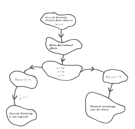
Figure 3: For $H(p,\rho,\nu)=0$, the extra-dimensional effects on the variables $(p,\rho,\nu)$, namely $(\delta\,p,\delta\rho,\delta\nu)$, do not produce any further anisotropy. Hence the anisotropy remains minimal onto the brane, and this is what ensures the low-energy limit is given by GR.

6 Matching condition for stellar distributions

An important aspect regarding the study of stellar distributions is the matching conditions at the star surface ($r=R$) between the interior ($r<R$) and the exterior ($r>R$) geometry.

In our case, the interior stellar geometry is given by the MGD metric

$$ds^{2}=e^{\nu^{-}(r)}\,dt^{2}-\left(1-\frac{2\,\tilde{m}(r)}{r}\right)^{-1}dr^{2}-r^{2}\left(d\theta^{2}+\sin{}^{2}\theta d\phi^{2}\right)\ ,$$ (6.1)

where the interior mass function is given by

$$\tilde{m}(r)=m(r)-\frac{r}{2}\,f^{*}(r)\ ,$$ (6.2)

with $m$ given by the standard GR expression (5.2) and $f^{*}$ the minimal geometric deformation in Eq. (5.10). Moreover, Eq. (5.10) implies that

$$f^{\ast}(r)\geq 0\ ,$$ (6.3)

so that the effective interior mass (6.2) is always reduced by the extra-dimensional effects.

The inner metric (6.1) should now be matched with an outer vacuum geometry, with $p^{+}=\rho^{+}=0$, but where we can in general have a Weyl fluid described by the scalars $\mathcal{U}^{+}$ and $\mathcal{P}^{+}$ [44]. The outer metric can be written as

$$ds^{2}=e^{\nu^{+}(r)}\,dt^{2}-e^{\lambda^{+}(r)}\,dr^{2}-r^{2}\left(d\theta^{2}+\sin{}^{2}\theta d\phi^{2}\right)\ ,$$ (6.4)

where the explicit form of the functions $\nu^{+}$ and $\lambda^{+}$ are obtained by solving the effective 4-dimensional vacuum Einstein equations

$$R_{\mu\nu}-\frac{1}{2}\,R^{\alpha}_{\ \alpha}\,g_{\mu\nu}=\mathcal{E}_{\mu\nu}\qquad\Rightarrow\qquad R^{\alpha}_{\ \alpha}=0\ ,$$ (6.5)

where we recall that extra-dimensional effects are contained in the projected Weyl tensor $\mathcal{E}_{\mu\nu}$. Only a few such analytical solutions are known to date [21, 22, 27, 44, 51]. Continuity of the first fundamental form at the star surface $\Sigma$ defined by $r=R$ reads

$$\left[ds^{2}\right]_{\Sigma}=0\ ,$$ (6.6)

where $[F]_{\Sigma}\equiv F(r\rightarrow R^{+})-F(r\rightarrow R^{-})\equiv F_{R}^{+}-F_{R}^{-}$, for any function $F=F(r)$, which yields

$${\nu^{-}(R)}={\nu^{+}(R)}\ ,$$ (6.7)

and

$$1-\frac{2\,M}{R}+f_{R}^{*}=e^{-\lambda^{+}(R)}\ ,$$ (6.8)

where $M=m(R)$. Likewise, continuity of the second fundamental form at the star surface reads

$$\left[G_{\mu\nu}\,r^{\nu}\right]_{\Sigma}=0\ ,$$ (6.9)

where $r_{\mu}$ is a unit radial vector. Using Eq. (6.9) and the general Einstein equations (3.1), we then find

$$\left[T_{\mu\nu}^{\rm eff}\,r^{\nu}\right]_{\Sigma}=0\ ,$$ (6.10)

which leads to

$$\left[p+\frac{1}{\sigma}\left(\frac{\rho^{2}}{2}+\rho\,p+\frac{2}{k^{4}}\,\mathcal{U}\right)+\frac{4\,\mathcal{P}}{k^{4}\,\sigma}\right]_{\Sigma}=0\ .$$ (6.11)

Since we assumed the star is only surrounded by a Weyl fluid characterised by $\mathcal{U}^{+}$, $\mathcal{P}^{+}$, this matching condition takes the final form

$$p_{R}+\frac{1}{\sigma}\left(\frac{\rho_{R}^{2}}{2}+\rho_{R}\,p_{R}+\frac{2}{k^{4}}\,\mathcal{U}_{R}^{-}\right)+\frac{4\,\mathcal{P}_{R}^{-}}{k^{4}\,\sigma}=\frac{2\,\mathcal{U}_{R}^{+}}{k^{4}\,\sigma}+\frac{4\,\mathcal{P}_{R}^{+}}{k^{4}\,\sigma}\ ,$$ (6.12)

where $p_{R}\equiv p^{-}(R)$ and $\rho_{R}\equiv\rho^{-}(R)$. Finally, by using Eqs. (4.2) and (5.11) in the condition (6.12), the second fundamental form can be written in terms of the MGD at the star surface, denoted by $f_{R}^{\ast}$, as

$$p_{R}+\frac{f_{R}^{*}}{k^{2}}\left(\frac{\nu_{R}^{\prime}}{R}+\frac{1}{R^{2}}\right)=\frac{2\,\mathcal{U}_{R}^{+}}{k^{4}\,\sigma}+\frac{4\,\mathcal{P}_{R}^{+}}{k^{4}\,\sigma}\ ,$$ (6.13)

where $\nu_{R}^{\prime}\equiv\partial_{r}\nu^{-}|_{r=R}$. Eqs. (6.7), (6.8) and (6.13) are the necessary and sufficient conditions for the matching of the interior MGD metric (6.1) to a spherically symmetric “vacuum” filled by a brane-world Weyl fluid.

The matching condition (6.13) yields an important result: if the outer geometry is given by the Schwarzschild metric, one must have $\mathcal{U}^{+}=\mathcal{P}^{+}=0$, which then leads to

$$p_{R}=-\frac{f_{R}^{\ast}}{k^{2}}\left(\frac{\nu_{R}^{\prime}}{R}+\frac{1}{R^{2}}\right)\ .$$ (6.14)

Given the positivity of $f^{*}$, Eq. (6.3), an outer Schwarzschild vacuum can only be supported in the brane-world by exotic stellar matter, with $p_{R}<0$ at the star surface.

7 The recipe

Let us conclude this brief introduction of the MGD approach by listing the basic steps to implement it:

Step 1:

pick a known perfect fluid solution $\{p,\rho,\nu\}$ of the conservation equation (3.16). This solution will ensure that $H(p,\rho,\nu)=0$ and the radial metric component $\lambda$ will be given by Eq. (5.1) with $f=f^{*}$ in Eq. (5.10). The GR solution will be recovered in the limit $\sigma^{-1}\to 0$ by construction.

Step 2:

determine the Weyl functions ${\cal P}$ and ${\cal U}$ from Eqs. (4.1) and (4.2).

Step 3:

use the second fundamental form given in Eq. (6.13) to express any GR constant $C$ as a function of the brane tension $\sigma$, that is, $C(\sigma)$. Then we are able to find the bulk effect on pressure $p$ and density $\rho$, that is, $p(\sigma)$ and $\rho(\sigma)$.

8 Conclusions

In the context of the Randall-Sundrum brane-world, a brief and detailed description of the basic elements of the MGD was presented. The explicit form of the anisotropic stress ${\cal P}$ was obtained in terms of the geometric deformation $f$ undergone by the radial metric component, thus showing the role played by this deformation as a source of anisotropy inside stellar distributions. It was shown that this geometric deformation is minimal when a GR solution is considered, therefore any perfect fluid solution in GR belongs to a subset of brane-world solutions producing a minimal anisotropy onto the brane. It was shown that with this approach it is possible to generate the brane-world version of any known GR solution, thus overcoming the non-closure problem of the effective 4-dimensional Einstein equations. A simple recipe showing the basic steps to implement the MGD approach was finally presented. A final natural question arises: is the MGD an useful approach to deal only with the effective 4-dimensional Einstein equations in the brane-world context? The answer is no. Indeed, we have found [52] that any modification of general relativity can be studied by the MGD provided that such modification can be represented by a traceless energy-momentum tensor. This mean that the MGD is particularly useful as long as the new gravitational sector is associated with a conformal gravitational sector.

Competing Interests

The authors declares that there is no conflict of interest regarding the publication of this paper.

9 Acknowledgements

A.S. is partially supported by Project Fondecyt 1161192, Chile.

References

- [1] B. P. Abbott et al. [LIGO Scientific and Virgo Collaborations], Phys. Rev. Lett. 116 (2016)no.6, 061102 [arXiv:1602.03837 [gr-qc]].
- [2] B. P. Abbott et al. [LIGO Scientific and Virgo Collaborations], Phys. Rev. Lett. 116 (2016)no.24, 241103 [arXiv:1606.04855 [gr-qc]].
- [3] Clifford M Will, Living Rev. Rel, 9 (2006).
- [4] Bergshoeff, Eric A; Hohm, Olaf; Townsend, Paul K, Massive Gravity in Three Dimensions Phys.Rev.Lett. 102: 201301 (2009); arXiv:0901.1766.
- [5] Claudia de Rham, Massive gravity Living Rev. Relativity 17,7 (2014); arXiv:1401.4173v2 [hep-th].
- [6] Eugeny Babichev, Kazuya Koyama, David Langlois, Ryo Saito, Jeremy Sakstein, Relativistic Stars in Beyond Horndeski Theories, Class. Quantum Grav. 33 235014 (2016); arXiv:1606.06627v3 [gr-qc].
- [7] Martin Krššák, Emmanuel N. Saridakis, The covariant formulation of f(T) gravity, Class. Quantum Grav. 33,115009 (2016); arXiv:1510.08432v2 [gr-qc].
- [8] Manuel Hohmann, Parameterized post-Newtonian limit of Horndeski’s gravity theory, Phys. Rev. D 92, 064019 (2015); arXiv:1506.04253v2 [gr-qc].
- [9] Nathan Chow, Justin Khoury, Galileon Cosmology, Phys.Rev.D 80, 024037 (2009); arXiv:0905.1325v4 [hep-th].
- [10] Antonio De Felice, Shinji Tsujikawa, f(R) theories, Living Rev. Rel. 13, 3 (2010); arXiv:1002.4928 [gr-qc].
- [11] Thomas P. Sotiriou and Valerio Faraoni, f(R) Theories of Gravity, Rev. Mod. Phys. 82, 451 (2010); arXiv:0805.1726 [gr-qc].
- [12] Sumanta Chakraborty and Soumitra SenGupta, Solving higher curvature gravity theories, Eur. Phys. J. C 76, 552 (2016); arXiv:1604.05301v2 [gr-qc].
- [13] Salvatore Capozziello, Mariafelicia De Laurentis, Extended Theories of Gravity, Phys.Rept. 509 (2011), 167 (2011); arXiv:1108.6266v2 [gr-qc].
- [14] S. Capozziello, Vincenzo F. Cardone, A. Troisi Reconciling dark energy models with f(R) theories, Phys.Rev. D 71, 043503 (2005); arXiv:astro-ph/0501426v1.
- [15] Timothy Clifton, Pedro G. Ferreira, Antonio Padilla, Constantinos Skordis, Modified Gravity and Cosmology,Phys.Rept. 513, 1 (2012); arXiv:1106.2476v3 [astro-ph.CO].
- [16] Petr Horava, Quantum Gravity at a Lifshitz Point, Phys.Rev.D 79, 084008 (2009); arXiv:0901.3775v2 [hep-th].
- [17] Jorge Bellorin, Alvaro Restuccia, On the consistency of the Horava Theory, Int.J.Mod.Phys. D21 1250029 (2012); arXiv:1004.0055 [hep-th].
- [18] J. Ovalle, Braneworld stars: anisotropy minimally projected onto the brane, in Gravitation and Astrophysics (ICGA9), Ed. J. Luo, World Scientific, Singapore, 173- 182 (2010); arXiv:0909.0531v2 [gr-qc].
- [19] L. Randall and R. Sundrum, A Large mass hierarchy from a small extra dimension, Phys. Rev. Lett. 83, 3370 (1999); arXiv:hep-ph/9905221v1.
- [20] L. Randall and R. Sundrum, An Alternative to compactification, Phys. Rev. Lett 83, 4690 (1999); arXiv:hep-th/9906064v1.
- [21] Roberto Casadio, Jorge Ovalle, Roldao da Rocha, The Minimal Geometric Deformation Approach Extended, Class. Quantum Grav. 32, 215020 (2015); arXiv:1503.02873v2 [gr-qc].
- [22] J Ovalle, Extending the geometric deformation: New black hole solutions, Int. J. Mod. Phys. Conf. Ser. 41 1660132 (2016); arXiv:1510.00855v2 [gr-qc].
- [23] J. Ovalle, Searching Exact Solutions for Compact Stars in Braneworld: a conjecture, Mod. Phys. Lett. A, 23, 3247 (2008); arXiv:gr-qc/0703095v3.
- [24] J. Ovalle, Non-uniform Braneworld Stars: an Exact Solution, Int. J. Mod. Phys. D, 18, 837 (2009); arXiv:0809.3547 [gr-qc].
- [25] J. Ovalle, The Schwarzschild’s Braneworld Solution, Mod. Phys. Lett. A, 25, 3323 (2010); arXiv:1009.3674 [gr-qc].
- [26] J. Ovalle, Effects of density gradients on brane-world stars, in Proceedings of the Twelfth Marcel Grossmann Meeting on General Relativity, eds. Thibault Damour, Robert T. Jantzen and Remo Ruffini. ISBN 978-981-4374-51-4. (World Scientific, Singapore, 2012), p.2243-2245
- [27] N. Dadhich, R. Maartens, P. Papadopoulos, V. Rezania, Black holes on the brane, Phys.Lett.B487,1-6(2000); arXiv:hep-th/0003061v3.
- [28] R. Casadio, J. Ovalle, Brane-world stars and (microscopic) black holes, Phys. Lett. B, 715, 251 (2012); arXiv:1201.6145 [gr-qc].
- [29] R. Casadio, J. Ovalle, Brane-world stars from minimal geometric deformation, and black holes, Gen. Relat. Grav., 46, 1669 (2014); arXiv:1212.0409v2 [gr-qc].
- [30] J. Ovalle, F. Linares, Tolman IV solution in the Randall-Sundrum Braneworld, Phys. Rev. D, 88, 104026 (2013); arXiv:1311.1844v1 [gr-qc].
- [31] J Ovalle, F Linares, A Pasqua, A Sotomayor, The role of exterior Weyl fluids on compact stellar structures in Randall-Sundrum gravity, Class. Quantum Grav., 30, 175019 (2013); arXiv:1304.5995v2 [gr-qc].
- [32] László Á. Gergely, Friedmann branes with variable tension, Phys.Rev.D78:084006 (2008); arXiv:0806.3857v3 [gr-qc].
- [33] R. Casadio, J. Ovalle, R. da Rocha, Black Strings from Minimal Geometric Deformation in a Variable Tension Brane-World, Class. Quantum Grav., 30, 175019 (2014); arXiv:1310.5853 [gr-qc].
- [34] J. Ovalle, L.A. Gergely, R. Casadio, Brane-world stars with solid crust and vacuum exterior, Class. Quantum Grav., 32, 045015 (2015); arXiv:1405.0252v2 [gr-qc].
- [35] R. Casadio, J. Ovalle, R. da Rocha, Classical Tests of General Relativity: Brane-World Sun from Minimal Geometric Deformation, Europhys. Lett., 110, 40003 (2015); arXiv:1503.02316 [gr-qc].
- [36] R. T. Cavalcanti, A. Goncalves da Silva, Roldao da Rocha, Strong deflection limit lensing effects in the minimal geometric deformation and Casadio–Fabbri–Mazzacurati solutions, Class. Quantum Grav. 33, 215007 (2016); arXiv:1605.01271v2 [gr-qc].
- [37] Roberto Casadio, Roldao da Rocha, Stability of the graviton Bose-Einstein condensate in the brane-world, Phys. Lett. B 763, 434 (2016); arXiv:1610.01572 [hep-th].
- [38] Roldao da Rocha, Dark SU(N) glueball stars on fluid branes, arXiv:1701.00761 [hep-ph].
- [39] Roldao da Rocha, Black hole acoustics in the minimal geometric deformation of a de Laval nozzle, arXiv:1703.01528 [hep-th].
- [40] D. Lovelock, J. Math. Phys. 12, 498 (1971).
- [41] R. Maartens, Brane-world gravity, Living Rev.Rel. 7 (2004).
- [42] R. Maartens, K. Koyama, Brane-world gravity, arXiv:1004.3962v1 [hep-th].
- [43] T. Shiromizu, K. Maeda and M. Sasaki, The Einstein Equations on the 3-Brane World, Phys.Rev. D 62 (2000) 024012; arXiv:gr-qc/9910076v3.
- [44] C. Germani, R. Maartens, Stars in the brane-world, Phys.Rev. D64, 124010(2001); arXiv:hep-th/0107011v3.
- [45] Tiberiu Harko, Matthew J. Lake, Null fluid collapse in brane world models, Phys. Rev. D 89, 064038 (2014); arXiv:1312.1420v3 [gr-qc].
- [46] Francisco X. Linares, Miguel A. Garcia-Aspeitia, L. Arturo Ureña-Lopez, Stellar models in Brane Worlds, Phys. Rev. D 92, 024037 (2015); arXiv:1501.04869v1 [gr-qc].
- [47] R. Casadio, L. Mazzacurati, Bulk shape of brane world black holes, Mod. Phys. Lett. A 18 (2003) 651-660 [arXiv:gr-qc/0205129v2].
- [48] R. da Rocha and J. M. Hoff da Silva, Black string corrections in variable tension brane-world scenarios, Phys. Rev. D 85, 046009 (2012) [arXiv:1202.1256v1 [gr-qc]].
- [49] K. Koyama and R. Maartens, Structure formation in the DGP cosmological model, JCAP 0601, 016 (2006); arXiv:astro-ph/0511634v1.
- [50] A. Viznyuk and Y. Shtanov, Spherically symmetric problem on the brane and galactic rotation curves, Phys.Rev.D,76 064009 (2007).
- [51] R. Casadio, A. Fabbri and L. Mazzacurati, New black holes in the brane world?, Phys. Rev. D 65, 084040 (2002), New black holes in the brane world?, gr-qc/0111072.
- [52] J. Ovalle, R. Casadio and A. Sotomayor, Searching for modified gravity: a conformal sector? ; arXiv:1702.05580 [gr-qc].