Direct Relation between the Excess Current Noise Spectral Density and the Complex Conductivity of Disordered Conductor
Abstract
We put forward a fundamental relationship between the normalized spectral density of excess current noise and the imaginary part of complex conductivity. In the case of metal our expression enables us to describe reliable experimental data on the excess noise giving nearly spectrum and correct temperature dependence of the Hooge factor. In the case of non-Debye conductors such as semiconductors and ionic glasses it leads to () for the excess noise spectrum. It is demonstrated that reactive ”capacitance” effects in electron conductivity are responsible for the excess current noise. The general relation that we introduce turns out to be a direct consequence of the continuous time random walk model.
pacs:
72.70.+m; 73.50.Td; 77.22.GmMany attempts have been made to explain the origin of excess current noise with the low-frequency spectrum on the background of direct current in various conducting materials 1 ; 2 ; 3 . It is believed to have been established that noise is determined by some relaxation processes accompanying the movement of carriers in disordered conductor. For example, in metals electrons are scattered by relaxing defect structures 4 ; 5 while in amorphous semiconductors and ionic glasses relaxation can be connected with trapping and hopping mechanisms of conductivity 6 ; 7 .
A broad distribution of relaxation times which usually have an activation form of dependence upon local energy barrier heights is very important for obtaining spectrum 1 ; 2 ; 3 . On the other hand, such a distribution inevitably leads to the low-frequency dependence (where and ) of ac conductivity 7 which is well-known for amorphous semiconductors and solid electrolytes 8 ; 9 ; 10 . Therefore, bearing in mind the common origin for both phenomena, one should expect the existence of some relation that links together the spectral density of the excess current noise and the frequency dependent complex conductivity in disordered conductors.
As it was stressed 10a for flicker noise there must exist ”… intimate connection with conductivity … a close relationship between the forms of the flicker noise and unsimulated noise…”. Previous attempts to establish it were called ”untenable” 2 .
In the present paper we find this relation with the help of the well-known continuous time random walk (CTRW) model 11 ; 12 ; 13 . Considering direct consequences of the revealed relation we demonstrate its applicability for the description of reliable experimental data. This allows one to make a conclusion that in spite of the model way of its derivation this relation is of fundamental nature.
Indeed, the CTRW model gives for the normalized excess current noise spectral density the expression
| (1) |
where is the noise spectral density, is the average current, is the number of carriers, is the Fourier transform 6 of the waiting-time distribution function and . The complex conductivity obtained in the CTRW model has the form 6
| (2) |
where is the conductivity at zero frequency (the so-called dc conductivity). From Eqs.(1) and (2) it immediately follows that
| (3) |
One may argue that the CTRW model we have used is oversimplified. However, those consequences from Eq.(3) that we obtain in the present work enables us to conclude that it is not restricted by the limitations of the CTRW model which Eq.(3) has been derived from.
To show this let us apply Eq.(3) to the case of metal with small concentration of randomly distributed point defects, where is the number density of the defects and is the number density of atoms. Let each single defect have states (for example, orientational ones 4 ; 5 ) which are characterized by different transport cross-sections () of electron scattering on a defect and let the number density of defects in th state be , so that
| (4) |
Following 5 we assume that transitions between the states of a defect occur through an energy barrier which contains the random component caused by non-uniform strain fields quenched in the polycrystal. We take for the Gaussian distribution function
| (5) |
where is some characteristic temperature for the quenched disorder 5 . Together with the activation form of relaxation times Eq.(5) leads to the log-normal distribution of these times.
Let us write down the real part of the complex conductivity for a high frequency (greater than inverse relaxation times but less than phonon frequencies). For this case all defect states can be considered randomly ”quenched” as far as electrons do not ”see” the changes in defect states. Then following 14
| (6) |
where beside the temperature-dependent contribution to resistivity from phonon- and electron-electron scattering there appear terms of residual resistivity 14 and we introduced ; is the Fermi momentum, is the electron charge, is the number density of electrons, . For metals 15 is a small expansion parameter so that having expanded Eq.(6) up to quadratic terms with respect to residual resistivity fluctuations we find
| (7) |
where we denoted - the total resistivity at , and
and we used the result of averaging over the random spatial distribution of defects 5 : .
Let us make it clear the origin of the difference between high and low frequency dependence of conductivity due to defects. For example, if one has a resistor network then at zero frequency the conductivity is determined by the average resistivity proportional to the successive sum of local resistivity in each part of the network. Just the quantity which is reciprocal to the average specific resistivity can be identified with the experimentally observable conductivity of such a system that is and brackets denote the abovesaid averaging. Meanwhile, the high frequency conductivity is a ”parallel channel” one in nature so that like in Eq.(6). These two quantities coincide only in the absence of spatial fluctuations of resistivity in the resistor network. These fluctuations are analogous of a defect distribution in the case of disordered metal.
Thus for our case at high frequency the increase in average conductivity is due to regions with low defect concentration (voids of low resistivity) unlike the dc case when the high and low resistivity regions sum up successively. It implies that reactive ”capacitance” effects in electron conductivity are the origin of the dispersion of the conductivity leading to the excess noise according to Eq.(3).
In the case of a distribution of relaxation times the defects with can be considered completely ”quenched” and the defects with - completely relaxed. Let us introduce the fraction of defects which can be ”seen” by conduction electrons as ”quenched” in their random states:
For high frequency and for low frequency it turns to zero.
Then we can generalize Eq.(7) for an arbitrary frequency
| (8) |
so that for Eq.(8) coincides with Eq.(7) and for it gives as it should be.
For the log-normal distribution function one can obtain
| (9) |
where erf is the error function, , and is the fluctuation exponent introduced in 7 . It is important for what follows that for K 5 and K 1 .
Let us introduce a function
| (10) |
investigated in 7 and for which in the limit there holds the formula
| (11) |
Taking into account Eqs.(9) and (11) one can rewrite Eq.(8) as
| (12) |
and after using the Kramers-Kronig relation 16 we have
| (13) |
It is worth noting that although the frequency dependent term in Eq.(12) is negligibly small comparatively to it is this term that gives all the effect in Eq.(13). Substituting Eq.(13) in Eq.(3) we finally have
| (14) |
This equation exactly coincides with the corresponding Eq.(27) from 5 (where Eq.(27) was derived by direct calculation of the temporal correlation function of resistivity) if one calculates taking into account the orientation modes of defects assumed in 5 . The important difference between Eq.(14) and Eq.(27) from 5 is that Eq.(14) is more general as to the assumptions made about the specific structure of defects. Namely, the Eq.(27) from 5 , in fact, describes the spectral density of anisotropic current fluctuations only. As far as Eq.(14) was studied in detail in 5 and was shown to give noise spectrum and a very accurate temperature dependence of the Hooge factor for metal we do not repeat these results here.
The other interesting and non-trivial case where Eq.(3) can be used is the case of strongly disordered conductors with a strong frequency dependence of , namely, amorphous semiconductors and ionic glasses. Here one should not expect a superposition form of Eq.(14) but has to use a general approach (e.g. the one developed in 7 for conductivity of ionic glasses) to calculate in matters with hopping conductivity.
The conductivity standing in Eq.(3) can be determined through the complex specific impedance calculated in 7 by the relation
| (15) |
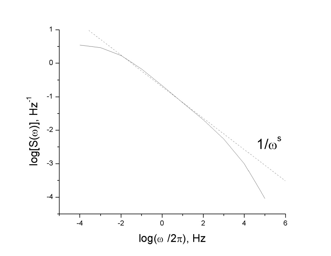
where is the high-frequency dielectric constant of the conductor and the complex conjugation was used to alter the sign before so that the definitions of Fourier transforms in Eq.(3) and in 7 are put in accordance. In Figure 1 we give for illustration the result of computation of obtained according to Eqs.(3) and (15) with taken from Eq.(37) in 7 . The parameters (so that corresponding according to Eq.(75) of 7 ), , and cm-1 chosen for the calculation are close to ordinarily used for ionic glasses. One can see from log-log scale Fig.1 that there exists the excess noise spectrum: (certainly, at very high frequencies it gives , not shown). For the parameters chosen here only the branch of type can be observable in experiment. It is interesting to notice that spectrum with was predicted in 17 ; 18 where it was discussed in relation with the non-Debye relaxation phenomena (see also 19 ; 20 where was found to be ). For semiconductors the value of for ac conductivity may be very close to unity.
It is useful to note that the tendency of the spectral density towards ”saturation” in the low-frequency limit (see Fig. 1) produces convergence of the noise integrated intensity, so the ”paradox” of the divergence of the mean square of the fluctuations of a quantity responsible for the noise frequently discussed in the literature (see, for example, the review 3 ) does not arise at all.
In conclusion, we have shown that there exists a relation given by Eq.(3) between the excess noise spectrum and the complex conductivity. This relation links together two phenomena previously considered separately, namely, the excess current noise and the frequency response in disordered conductors. In spite of the fact that this relation has been established with the help of the CTRW model we claim that it is fundamental and there are some weighty reasons to find its proof on the basis of general physical principles. We believe that our relation breaks ”… a long tradition of models being proposed that are forgotten after a short time.” (see 17 where these words of F.N. Hooge were cited) .
Acknowledgements.
I would like to thank Prof. M.B. Weissman for helpful discussions.References
- (1) E-mail: peter@snu.ac.kr
- (2) P. Dutta and P.M. Horn, Rev. Mod. Phys. 53, 497 (1981).
- (3) M.B. Weissman, Rev. Mod. Phys., 60, 537 (1988).
- (4) Sh.M. Kogan, Usp. Fiz. Nauk, 145, 285 (1985) [ Sov. Phys. - Usp., 28, 170 (1985)].
- (5) Sh.M. Kogan and K.E. Nagaev, Fiz. Tverd. Tela, 24, 3381 (1982) [Sov. Phys. - Solid State, 24, 1921 (1982)].
- (6) V.N. Bondarev and P.V. Pikhitsa, J. Phys.: Cond. Matter, 10, 6735 (1998).
- (7) H. Sher and M. Lax, Phys. Rev. B, 7, 4491 (1973).
- (8) V.N. Bondarev and P.V. Pikhitsa, Phys. Rev. B, 54, 3932 (1996).
- (9) K. Pollak and T.H. Geballe, Phys. Rev., 122, 1742 (1961).
- (10) S. Summerfield, Phil. Mag. B, 52, 9 (1985).
- (11) A.K. Jonscher, Phys. Status Solidi A, 32, 665 (1975).
- (12) A.G. Hunt, J. Phys.:Cond. Matter, 10, L303 (1998).
- (13) J.K.E. Tunaley, J. Stat. Phys., 15, 149 (1976).
- (14) M. Nelkin and A.K. Harrison, Phys. Rev. B, 26, 6696 (1982).
- (15) C.J.Staton and M. Nelkin, J. Stat. Phys., 37, 1 (1984).
- (16) E.M. Lifshitz and L.P. Pitaevskii, Physical Kinetics (Nauka: Moscow, 1979) [in Russian].
- (17) A.C. Damask and G.J. Dienes, Point Defects in Metals (NY: Gordon and Breach, 1963).
- (18) L.D. Landau, E.M. Lifshitz, Statistical Physics, part 1 (Nauka, Moscow, 1976) [in Russian].
- (19) K.L. Ngai, Phys. Rev. B, 22, 2066 (1980).
- (20) M.B. Weissman, Phys. Rev. Lett., 59, 1772 (1987).
- (21) Sh. M. Kogan and B.I. Shklovskii, Fiz. Tekh. Poluprov., 15, 1049 (1981) [in Russian].
- (22) W. Lehr, J. Machta and M. Nelkin, J. Stat. Phys., 36, 15 (1984).