The dark side of solar photospheric G-band bright points

Bright small-scale magnetic elements found mainly in intergranular lanes at the solar surface are named bright points (BPs). They show high contrasts in Fraunhofer G-band observations and are described by nearly vertical slender flux tubes or sheets. A recent comparison between BP observations in the ultraviolet (UV) and visible spectral range recorded with the balloon-borne observatory Sunrise and state-of-the-art magnetohydrodynamical (MHD) simulations revealed a kiloGauss magnetic field for 98% of the synthetic BPs. Here we address the opposite question, namely which fraction of pixels hosting kiloGauss fields coincides with an enhanced G-band brightness. We carried out 3D radiation MHD simulations for three magnetic activity levels (corresponding to the quiet Sun, weak and strong plage) and performed a full spectral line synthesis in the G-band. Only 7% of the kiloGauss pixels in our quiet-Sun simulation coincide with a brightness lower than the mean quiet-Sun intensity, while 23% of the pixels in the weak-plage simulation and even 49% in the strong-plage simulation are associated with a local darkening. Dark strong-field regions are preferentially found in the cores of larger flux patches that are rare in the quiet Sun, but more common in plage regions, often in the vertices of granulation cells. The significant brightness shortfall in the core of larger flux patches coincide with a slight magnetic field weakening. KiloGauss elements in the quiet Sun are on average brighter than similar features in plage regions. Almost all strong-field pixels display a more or less vertical magnetic field orientation. Hence in the quiet Sun, G-band BPs correspond almost one-to-one with kiloGauss elements. In weak plage the correspondence is still very good, but not perfect.

1 Introduction

Photospheric bright points (BPs) are small-scale brightness enhancements usually formed in intergranular lanes on the Sun’s surface. They were first observed by Dunn & Zirker (1973) in H$\alpha$ line wing images and later by Mehltretter (1974) who, from a comparison between Ca ii K images with a Kitt Peak magnetogram, concluded that BPs are magnetic structures. With sizes between 70 km and 600 km (Berger et al., 1995; Sánchez Almeida et al., 2004; Beck et al., 2007; Utz et al., 2009; Keys et al., 2013; Riethmüller et al., 2014) they belong to the smallest known magnetic features and often they are right at or even below the resolution limit of modern solar telescopes. They typically live for a few 100 s (Muller, 1983; Sánchez Almeida et al., 2004; Keys et al., 2011; Jafarzadeh et al., 2013; Keys et al., 2014). The physical structure underlying BPs are magnetic elements, which in general have kiloGauss field strengths (e.g., Stenflo, 1973; Rabin, 1992; Rüedi et al., 1992; Riethmüller et al., 2014).

Over a solar activity cycle the contribution of the brightness excess of magnetic elements to solar irradiance is believed to overcompensate the darkening produced by sunspots (Krivova et al., 2003; Domingo et al., 2009; Fröhlich, 2013; Solanki et al., 2013). Hence the magnetic elements are thought to be responsible for an increased total solar irradiance (TSI) during magnetic activity maxima of the Sun (Willson & Hudson, 1988). The influence of TSI variations (on time scales of decades or more) on the terrestrial climate is under debate (London, 1994; Larkin et al., 2000; Gray et al., 2010; Haigh et al., 2010; Ermolli et al., 2013). In particular the variations in the ultraviolet (UV) are much larger than for longer wavelengths (Krivova et al., 2006; Harder et al., 2009) and hence the UV properties of BPs are of great potential importance (Riethmüller et al., 2010). However, many of their properties are not known with sufficient accuracy.

Criscuoli & Uitenbroek (2014) studied G-band BPs in MHD simulations of the Stagger code (Galsgaard & Nordlund, 1996) and determined a bimodal distribution of their magnetic field strength. The first peak below 100 G corresponds to bright granules misidentified as BPs and the second at about 1500 G to magnetic features. Utz et al. (2013) detected BPs in G-band observations recorded with the Solar Optical Telescope aboard the Hinode satellite (Tsuneta et al., 2008) and retrieved their field strength distribution from Milne-Eddington inversions of simultaneously acquired spectropolarimetric data. They also found bimodal distributions of the field strength for the BPs, both in the quiet Sun and in an active region.

Similarly Riethmüller et al. (2014) reported that in an MHD simulation with an averaged field strength of 30 G at the solar surface, representative of the quiet Sun, 98% of the synthetic BPs harbor kiloGauss field strengths. They also carefully compared a number of spectropolarimetric parameters in the MHD simulation with those in high-resolution observations obtained by the IMaX instrument (Martínez Pillet et al., 2011) on the Sunrise balloon-borne observatory (Solanki et al., 2010; Barthol et al., 2011; Berkefeld et al., 2011; Gandorfer et al., 2011). This comparison showed that both can be reconciled if spatial and spectral degradation due to the instrument is meticulously taken into account.

Here we follow up on this work by considering the opposite question: Do all quiet-Sun kiloGauss elements lead to bright features or are there small dark, strong-field features as well? We note that Riethmüller et al. (2014) concentrated on degraded MHD data (in order to allow direct comparisons with the observations), while we now focus on undegraded MHD data that are noise-free and have high spatial resolution. We are able to do that since the validity of the simulations was already tested versus seeing-free observations by Riethmüller et al. (2014).

2 Simulation and spectral synthesis

We used the MURaM code for realistic simulations of the radiative and magneto-hydrodynamical processes in the solar photosphere and the uppermost layers of the convection zone. MURaM is a three-dimensional, non-ideal, compressible MHD code, which includes non-gray calculations of the radiative transfer of energy under the assumption of local thermal equilibrium (Vögler et al., 2005). At the bottom boundary of the simulation box a free in- and outflow of matter was allowed under the constraint of total mass conservation, while at the upper boundary the vertical convective fluxes of mass, energy and horizontal momentum vanish, and the magnetic field lines are assumed to be vertical. In the horizontal directions we used periodic boundary conditions. Our simulation box covers 6 Mm $\times$ 6 Mm in the horizontal directions, with a cell size of 10.4 km, while it covers 1.4 Mm in the vertical direction, with a 14 km cell size. On average, optical depth unity for the continuum at 500 nm is reached 500 km below the upper boundary of the box.

Our initial condition was a statistically relaxed purely hydrodynamical simulation in which we introduced a unipolar homogeneous vertical magnetic field, $\langle B_{\rm{z}}\rangle$. To reach a statistically stationary state again, we ran the simulation for a further 3 hours of solar time. Ten snapshots were then analyzed for each simulation run, one every 5 minutes of solar time, so that the snapshots can be considered to be nearly statistically independent. For this study we calculated ten snapshots taken from a simulation run with an initial $\langle B_{\rm{z}}\rangle=30$ G (simulating a quiet-Sun region), another ten snapshots with $\langle B_{\rm{z}}\rangle=200$ G (simulating a weak plage region), and finally ten snapshots with $\langle B_{\rm{z}}\rangle=400$ G (strong plage). More details about the MHD simulation runs analyzed here can be found in Riethmüller et al. (2014).

The SPINOR inversion code was used in its forward computation mode (Solanki, 1987; Frutiger, 2000; Frutiger et al., 2000) to compute synthetic Stokes spectra of the G-band, a spectral range around 430.5 nm dominated by lines of the CH molecule. This spectral range was selected since G-band brightenings have been used as proxies of small-scale magnetic features for a long time and a wealth of observations are available (e.g., Muller & Roudier, 1984; Berger et al., 1995; Title & Berger, 1996; Wiehr et al., 2004; Zakharov et al., 2005; Beck et al., 2007; Berger et al., 2007; Bonet et al., 2012; Keys et al., 2014). We used a Lorentz profile having a full width at half maximum (FWHM) of 1 nm as a typical filter transmission profile, multiplied it point by point with the synthetic intensity profiles, and summed up the products. These scaler products gave the G-band intensity at a spatial pixel of a synthetic image. Additional information about the spectral synthesis of the G-band can be found in Shelyag et al. (2004), cf. Schüssler et al. (2003). All computations refer to the center of the solar disk.

3 Results

3.1 Relationship between intensity and magnetic field strength

3.1.1 Full spatial resolution

Scatter plots of the G-band intensity versus the magnetic field strength are displayed in Fig. 1 (black dots). All pixels of all snapshots contributed to this figure (576 pixels $\times$ 576 pixels $\times$ 10 snapshots). A binning of the scatter plots was applied by averaging groups of 5000 data points with similar $B$ (cyan lines in Fig. 1). The binned brightness drops below the mean quiet-Sun value, $I_{\rm{QS}}$ (taken to be the average intensity of the 30 G simulation), for intermediate field strengths, before it rises to well above this value for kiloGauss fields. The scatter in intensity for the kiloGauss fields increases considerably with $\langle B_{\rm{z}}\rangle$. The magnetic field strength, used to produce the scatter plots, was taken at an optical depth of $\log(\tau)=-1$ because field strengths retrieved by Milne Eddington inversions of, e.g., the Fe i 525.02 nm line correspond to roughly this optical depth (Orozco Suárez et al., 2010).

This choice also allows a direct comparison of our 200 G simulation (middle panel of Fig. 1) with the one carried out by Shelyag et al. (2004) (see the left panel of their Fig. 4). These authors calculated MURaM snapshots for an initial $\langle B_{\rm{z}}\rangle$ of 200 G, but used a coarser computational grid with a cell size of 20.8 km in both horizontal directions. The qualitative behavior of their scatter plot is very similar to ours. They found a maximum field strength of 2700 G, which is also quite close to the value of 2600 G that we retrieved from our 200 G simulation. In contrast to these agreements, Shelyag et al. (2004) found a maximum G-band intensity value of 2.2 times the mean quiet-Sun value, while we obtain a considerably higher value of $3.8\,I_{\rm{QS}}$. Shelyag et al. (2004) also considered a 10 G simulation as quiet-Sun reference and found a maximum field strength of 1900 G and a maximum G-band intensity of 1.6 $I_{\rm{QS}}$, while we used an averaged field strength of 30 G to simulate the quiet Sun and found 2300 G and 3.4 $I_{\rm{QS}}$ as the maximum values, but this time a direct comparison is difficult because both, the mean vertical field strength and the cell size are different between the simulations.

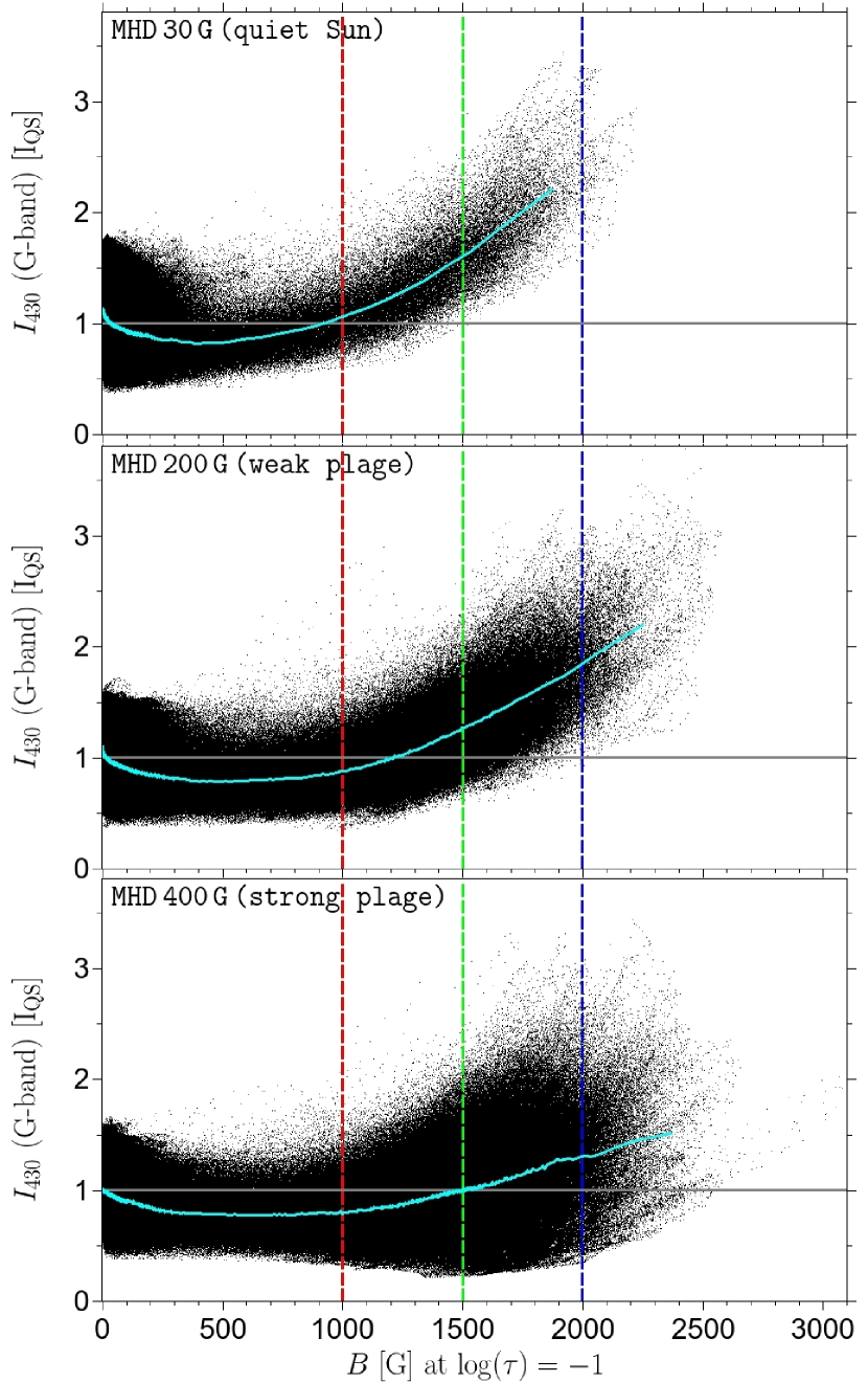
Figure 1: Scatter plots of the G-band intensity versus the magnetic field strength at $\log(\tau)=-1$ (black dots). The cyan lines connect binned values. The top, middle, and bottom panel corresponds to MHD simulations with an initial mean vertical flux density of 30 G, 200 G, and 400 G, respectively. The horizontal line in each frame marks the mean quiet-Sun intensity and the vertical lines indicate field strengths of 1000 G, 1500 G, and 2000 G.

A comparison between our quiet-Sun simulation (top panel of Fig. 1) and our plage simulations (middle and bottom panels of Fig. 1) reveals not just that there are many more pixels with kiloGauss fields in the latter, but that these pixels are on average also somewhat less bright. Thus, the fraction of pixels possessing an intensity lower than $I_{\rm{QS}}$ (below the gray horizontal line) and a kiloGauss magnetic field (right of the red vertical line) increases from 0.13% for the quiet-Sun simulation to 4.2% for the weak-plage simulation and to 15.8% for the strong-plage simulation. For a magnetic field threshold of 1500 G (green vertical line) we find no dark pixels anymore in the quiet-Sun snapshots but still 0.24% (4.6%) of all pixels of the weak- (strong-) plage simulation.

To get a better insight into this effect we calculated G-band intensity histograms of only those pixels whose magnetic field strength exceeds a certain threshold, $B_{T}$. These histograms, $H_{B_{T}}(I_{430})$, are then integrated over the intensity

$$F_{B_{T}}(I_{430})=\frac{1}{N_{B_{T}}}\int\limits_{I_{430}}^{\infty}H_{B_{T}}(I_{430}^{\prime})\,dI_{430}^{\prime},$$ (1)

where $1/N_{B_{T}}$ implies normalization to the total number of pixels that harbor a field strength of at least $B_{T}$,

$$N_{B_{T}}=\int\limits_{0}^{\infty}H_{B_{T}}(I_{430}^{\prime})\,dI_{430}^{\prime},$$ (2)

so that $F_{B_{T}}(I_{430})$ gives the fraction of strong-field pixels having a G-band intensity of at least $I_{430}$.

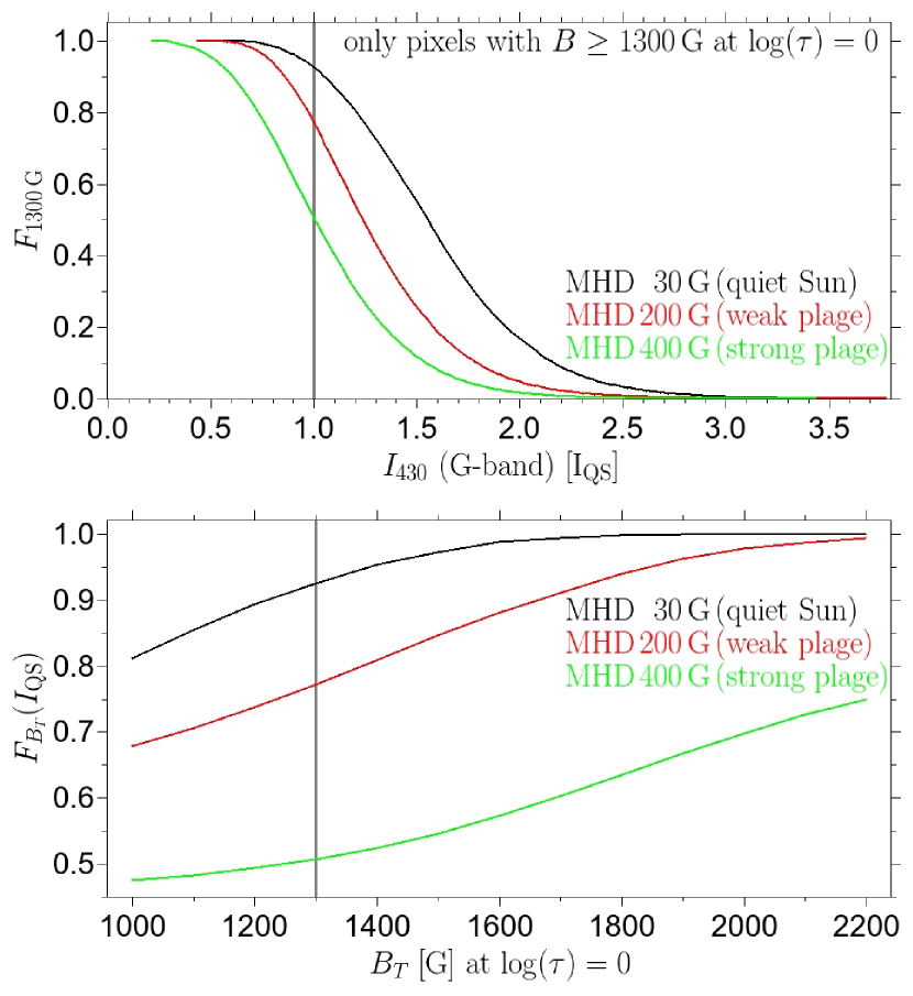
Figure 2: Top panel: Integrated G-band intensity histograms, $F_{B_{T}}$, of strong-field pixels with $B\geq 1300$ G (see main text for definition). The mean quiet-Sun intensity is indicated by the vertical line. Bottom panel: Variation of $F_{B_{T}}(I_{\rm{QS}})$ with $B_{T}$, where $I_{\rm{QS}}$ is the mean quiet-Sun intensity and $B_{T}$ is the magnetic field threshold. $F_{B_{T}}(I_{\rm{QS}})$ gives the fraction of all pixels having a field strength greater than $B_{T}$, which also have an intensity greater than $I_{\rm{QS}}$. The vertical line indicates the lowest $B_{T}$ value at optical depth unity that corresponds to a kiloGauss field at the height of average line formation of Fe i 525.02 nm. The black, red, and green lines refer to the snapshots taken from the 30 G, 200 G, and 400 G simulation.

Since the gas pressure decreases with height in the solar photosphere, flux tubes expand with height and form a canopy. This is a region where a vertical ray coming from the top passes through the magnetized atmosphere of the expanding flux tube in the upper photosphere, then hits the nearly field-free atmosphere below the canopy before penetrating the $\tau=1$ surface and entering the solar interior (e.g., Solanki, 1989). Such rays often show a kiloGauss field combined with a low brightness due to the location of magnetic elements in intergranular lanes. By limiting our analysis to pixels harboring kiloGauss field strengths at the $\tau=1$ surface we excluded pixels in the canopy. A scatter plot of the magnetic field strength at $\log(\tau)=0$ versus the field strength at $\log(\tau)=-1$ taken from our quiet-Sun simulation (not shown) revealed that on average a field strength at optical depth unity of at least 1300 G is needed to reach kiloGauss field strengths at $\log(\tau)=-1$, i.e. at the optical depth to which the field strengths retrieved by Milne Eddington inversions of the Fe i 525.02 nm line refer to.

The top panel of Fig. 2 displays $F_{B_{T}}(I_{430})$ for a magnetic field threshold at optical depth unity of $B_{T}=1300$ G. These strong-field pixels of the 30 G, 200 G, and 400 G simulation cover an intensity range of $0.54\,I_{\rm{QS}}-3.44\,I_{\rm{QS}}$, $0.43\,I_{\rm{QS}}-3.78\,I_{\rm{QS}}$, and $0.22\,I_{\rm{QS}}-3.45\,I_{\rm{QS}}$, respectively. 93% of the kiloGauss pixels of the 30 G snapshots reach an intensity higher than the mean quiet Sun, but only 77% of the kiloGauss pixels of the 200 G snapshots and just 51% of the 400 G simulation. We note that a fraction of 93% in the quiet-Sun simulation means that 7% of the kiloGauss pixels are darker than the mean quiet Sun. This fraction is equivalent to 0.06% of all pixels (including pixels of any field strength) and hence lower than the 0.13% mentioned above because we here exclude the dark canopy pixels. We also plotted $F_{1000\,\mathrm{G}}(I_{430})$, $F_{1500\,\mathrm{G}}(I_{430})$, and $F_{2000\,\mathrm{G}}(I_{430})$ (not shown) and found that the upper limit of the intensity ranges is not influenced by $B_{T}$ because the brightest pixels always possess very strong fields. The lower limit of the intensity ranges as well as the difference between the curves for the three simulations increases with $B_{T}$.

In the bottom panel of Fig. 2 we show the variation of the $F_{B_{T}}$ value with $B_{T}$ at the constant mean quiet-Sun intensity, $I_{430}=I_{\rm{QS}}$, i.e. it shows the fraction of pixels with $B>B_{T}$ that have $I>I_{\rm{QS}}$. Generally, the fraction of strong-field pixels reaching intensities higher than $I_{\rm{QS}}$ is larger in our quiet-Sun simulation than in our plage simulations. For the lower part of the displayed $B_{T}$ range the $F_{B_{T}}$ curves increase roughly linearly, while in the kiloGauss range the curves approach asymptotically the value 1. The smoothness of the three curves shows that the fraction of strong-field pixels having over-average brightnesses that we retrieved from our analysis depends smoothly on the chosen $B_{T}$ threshold.

3.1.2 Reduced spatial resolution

To demonstrate the influence of the spatial resolution on the fraction of strong-field pixels in the form of G-band BPs, we convolved the G-band images with an Airy function that corresponds to the G-band wavelength, 430.5 nm, and to a circular telescope aperture of diameter $D=0.5$ m (e.g. Hinode/SOT), $D=1$ m (Sunrise, SST), $D=1.5$ m (Gregor, NST), and $D=4$ m (DKIST), respectively. As an example, we plot the integrated histograms of the $D=0.5$ m case in Fig. 3. Qualitatively, the curves for the three magnetic types of simulation show a behavior similiar to the undegraded case displayed in the top panel of Fig. 2. The degradation squeezes the curves towards lower intensities, so that the fractions of strong-field pixels having $I>I_{\rm{QS}}$ become smaller (intersections with the vertical line).

The dependence of the fractions on the level of degradation is given in Table 1 and shows that the diffraction limit of a 4 m telescope hardly affects the fraction of kiloGauss pixels, while the reduction for a 1 m or an even smaller telescope is significant. We note that the cell size of our simulations corresponds roughly to half the diffraction limit of a 4 m telescope in the G-band spectral range, so that a significant influence of a 4 m telescope diffraction on the fraction of kiloGauss pixels in a simulation with a cell size smaller than 10 km cannot be ruled out.

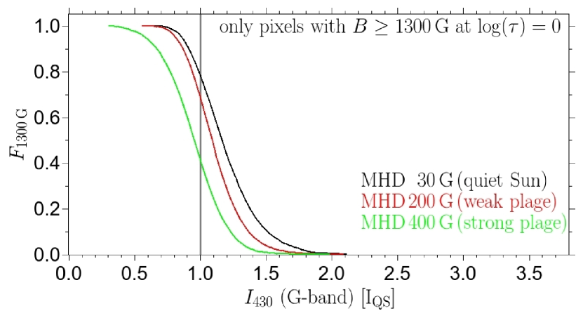
Figure 3: Same as the top panel of Fig. 2 but for G-band data degraded to the diffraction limit of a 0.5 m telescope.

Table 1: Fraction of kiloGauss field in the form of G-band bright points for various telescope sizes.

Degradation	30 G	200 G	400 G
	(quiet Sun)	(weak plage)	(strong plage)
undegraded	0.93	0.77	0.51
4.0 m telescope	0.92	0.77	0.50
1.5 m telescope	0.91	0.76	0.48
1.0 m telescope	0.88	0.74	0.47
0.5 m telescope	0.78	0.68	0.41

Fig. 4 displays the influence of the diffration at the aperture of a 0.5 m telescope on a G-band intensity image of a kiloGauss element extended from 0.6 to 1.5 Mm in x direction and from 1.1 to 1.4 Mm in y direction (see the left panel of Fig. 4). The undegraded G-band intensity is mainly below the quiet-Sun average in the central part of the magnetic feature, while being mostly above the quiet-Sun average in the periphery of the feature, in particular at its left as well as its bottom-right edge. Nonetheless, at full spatial resolution the magnetic feature can be recognized as a single entity (see the middle panel of Fig. 4). This changes when the feature is observed with a 0.5 m telescope (see the right panel of Fig. 4). At the reduced spatial resolution the feature appears as three isolated small BPs around the positions (0.7 Mm,1.3 Mm), (1.1 Mm,1.2 Mm), and (1.4 Mm,1.2 Mm), while the dark central part of the feature can no longer be recognized as belonging to the entity.

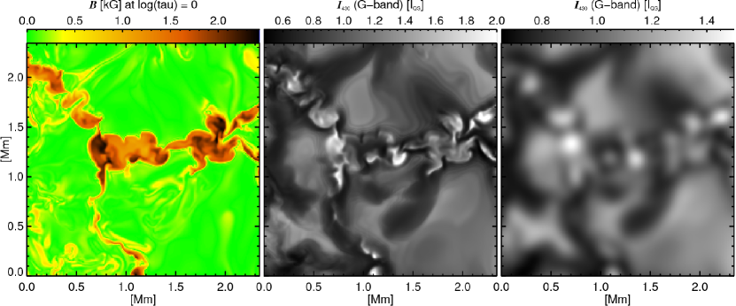
Figure 4: Magnetic field strength at optical depth unity (left panel), G-band intensity at full spatial resolution (middle panel) and as seen by an ideal 0.5 m telescope (right panel) of a magnetic element of the 200 G simulation harboring bright and dark strong-field pixels.

3.2 Dark strong-field regions

3.2.1 Locations within the convection pattern

Figures 1 and  2 reveal that even if the majority of kiloGauss pixels are brighter than the mean quiet Sun, a non-negligible fraction of them is dark. Here we analyze where those dark pixels are located within the solar granulation pattern. In Fig. 5 we show a G-band intensity map (top panel) and a map of the magnetic field strength at optical depth unity (bottom panel) of one of the weak-plage, 200 G, snapshots. In agreement with earlier studies, these images show that strong-field regions are predominantly located in intergranular lanes, in particular the largest ones are often found at the vertices of three or more granulation cells. We over-plotted contour lines that indicate regions darker than the mean quiet Sun where the field strength is at least 1 kG. These regions are mainly located in the cores of larger flux patches with horizontal sizes of $200-500$ km (at their narrowest points), see, e.g., the patches at $(x,y)=(3.0\,\rm{Mm},\,5.1\,\rm{Mm})$ and $(3.2\,\rm{Mm},\,2.3\,\rm{Mm})$. In addition to these larger dark patches there are also smaller dark strong-field regions. These are preferentially found at the edges of flux patches, most probably because the G-band intensity is mainly formed somewhat higher than optical depth unity so that an inclination of the magnetic field can lead to a slight mismatch between the magnetic and the brightness structure.

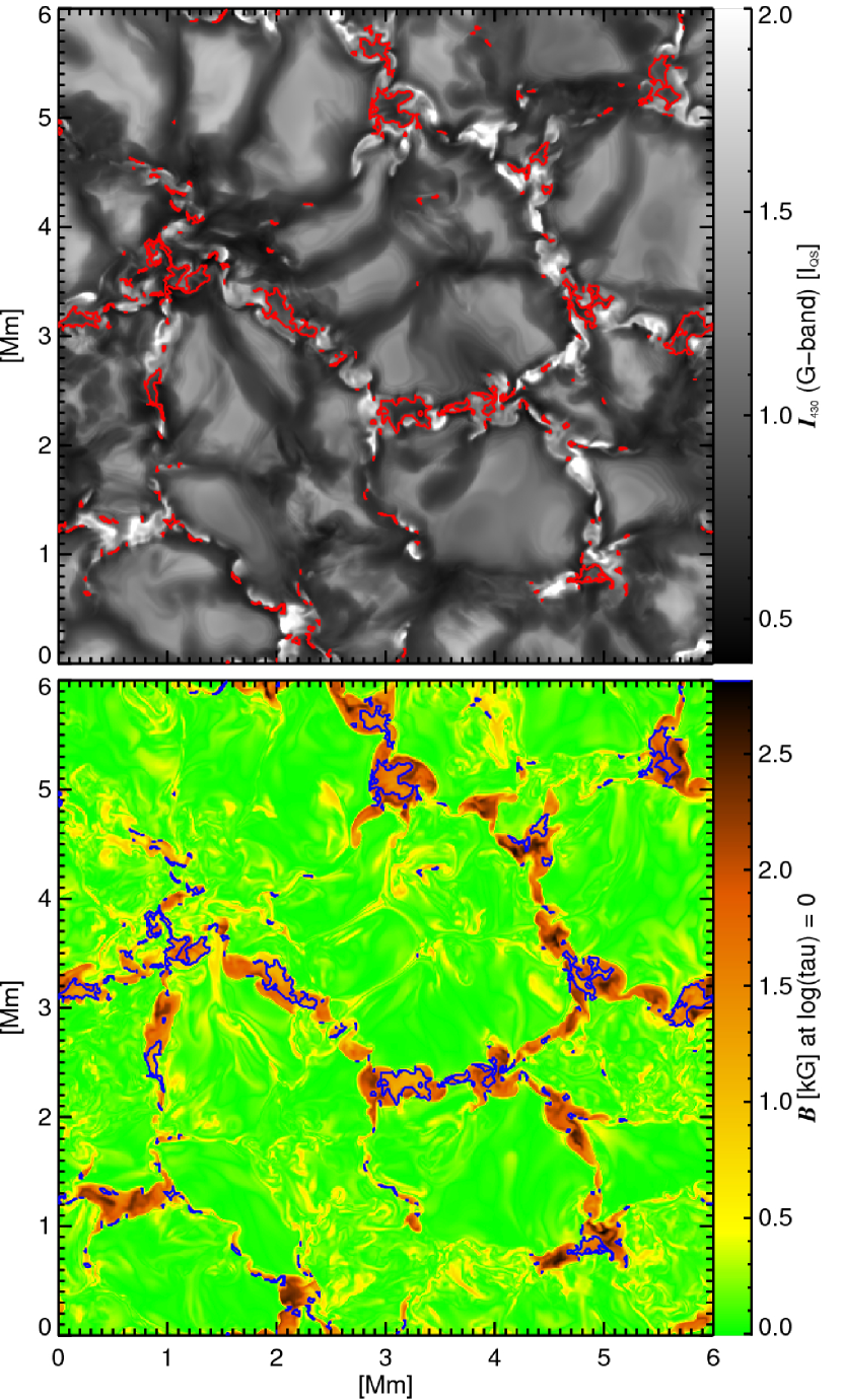
Figure 5: G-band intensity (top panel) and magnetic field strength at optical depth unity (bottom panel) of a 200 G MHD simulation. The contour lines (red in the top panel and blue in the bottom panel) indicate dark, strong-field regions, i.e. $I_{\rm{430}}<I_{\rm{QS}}$ and $B_{\rm{\tau=1}}>1000$ G. The intensities of the G-band image are saturated at $2\,I_{\rm{QS}}$ for a better visibility of the granulation pattern.

3.2.2 Magnetic field weakening

Often not only the intensity in the interior of large flux patches drops, but surprisingly also a slight magnetic field weakening can be found at these places (see the bottom panel of Fig. 5). More insight into such magnetic field weakening in the interiors of large flux patches can be gained from Fig. 6, which shows, among other things, vertical cuts through the flux patch at $(x,y)=(3.0\,\rm{Mm},\,5.1\,\rm{Mm})$ in Fig. 5 along the horizontal line shown in panels a-h of Fig. 6. Both the G-band (panel a) and bolometric intensity (panel e) exhibit a clearly reduced brightness in the interior of the flux patch. The two intensity profiles (panel i) display a similar behavior, but the intensity contrast is considerably higher in the G-band, the main reason why G-band observations are frequently used. The temperature profile at optical depth unity (blue line in panel j) more or less follows the intensity profiles, while the temperature profile at zero geometrical height (green line in panel j) displays a significant depression that coincides with an enhanced magnetic field strength (panel k). The optical depth unity surface (e.g., white line in panel m) exhibits a clear Wilson depression, as expected for strong-field regions. The magnetic field weakening in the magnetic feature’s interior is not only visible in the map at constant optical depth (panel c) but also in the map at constant geometrical height (panel g).

The vertical cut in panel n conspicuously shows the flux-tube expansion above the $\tau=1$ line. The vertical cut also reveals that the magnetic field strength is rather inhomogeneously distributed across the flux tube. Compared with the strongest magnetic fields of around 2300 G at $x=475$ to $575\,\rm{km}$ the field strength at $x=300$ to $400\,\rm{km}$ is only around 1400 G. The weaker field is associated with a lower magnetic pressure which is approximately balanced by a higher gas pressure. This in turn is accompanied by a higher density and hence a raised $\tau=1$ level. Accordingly, the $\tau=1$ line is located at lower temperatures compared with the adjacent region and hence the region is darker. The same mechanism appears to be acting also in the other bigger dark patches.

Horizontal maps of the line-of-sight (LOS) velocity (panels d and h of Fig. 6) display downflow lanes surrounding the dark strong-field regions. These downflow lanes are narrower in the map at constant geometrical height. They are narrow but somewhat inclined with height, so that they appear broader at constant optical depth because of the sampling of a range of heights. While the majority of pixels in the dark strong-field region shown in the centers of the panels of Fig. 6 displays upflows, this in not always the case. Other dark strong-field regions usually harbour downflows or both, up- and downflows. The vertical cut in panel o exhibits a quite inhomogeneous velocity distribution with both upflows and downflows inside the flux patch. The strongest downflows are located at the edges of the strong-field magnetic feature and are the downflow lanes in which the feature is embedded. The strongest upflows coincide with the strongest magnetic field, although the weaker, darker field is also associated with an upflow. The transition between strong upflow and downflow regions does not lead to any distinctive feature in intensity.

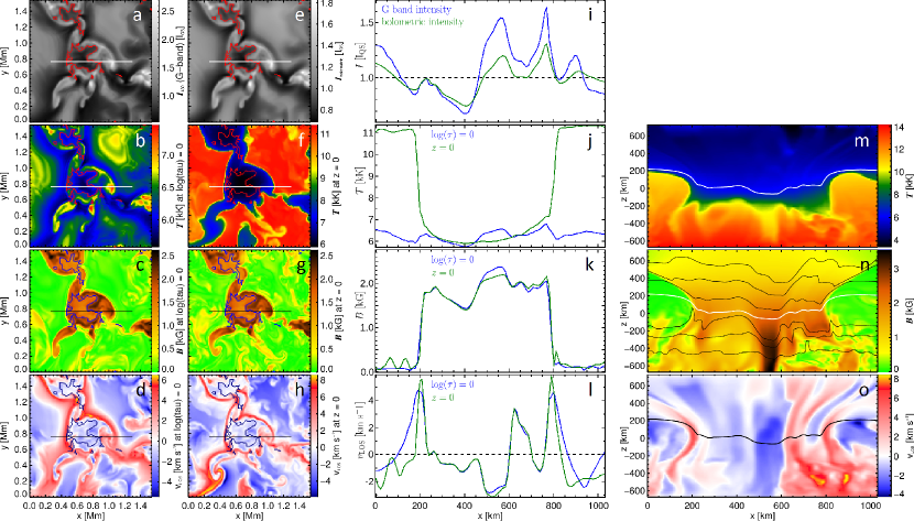
Figure 6: Maps of the G-band intensity (panel a), bolomeric intensity (panel e), temperature, magnetic field strength, and line-of-sight velocity at optical depth unity (panels b-d) and at constant geometrical height zero (panels f-h) of the flux patch at $(x,y)=(3.0\,\rm{Mm},\,5.1\,\rm{Mm})$ in Fig. 5. Contour lines are the same as in Fig. 5. The horizontal lines mark the position of the profiles plotted in panels i-l (blue lines for the first column of panels a-d and green lines for the second column of panels e-h) and the vertical cuts displayed in panels m-o. The optical depth unity level is marked by a white line in panels m and n and as a black line in panel o. The black lines in panel n are iso-density lines. Negative velocities correspond to upflows.

3.3 Relation between magnetic field strength and inclination

Finally, we calculated a two-dimensional histogram of the magnetic field strength and field inclination of all pixels of the weak-plage simulation at optical depth unity (Fig. 7). We found a bimodal distribution whose first population peaks at (30 G, $86^{\circ}$), i.e. for almost horizontally oriented, very weak fields, while the second populaton has its peak at (1700 G, $5^{\circ}$), i.e. for almost vertical strong fields. While the strong-field population displays a relatively narrow range of field inclinations (roughly between $0^{\circ}$-$20^{\circ}$), the angular distribution becomes asymptotically isotropic towards zero field strength. We also calculated such two-dimensional histograms for the optical depths $\log(\tau)=-1$ and $-2$ (not shown). While the position of the weak-field peak does not change much with optical depth, the position of the strong-field peak depends considerably on the optical depth, being at (1400 G, $7^{\circ}$) and (880 G, $13^{\circ}$) for $\log(\tau)=-1$ and $-2$, respectively. We note that the magnetic field distributions of our quiet-Sun simulation (not shown) also have a bimodal character, but because of the fewer strong-field pixels the strong-field population is much less pronounced.

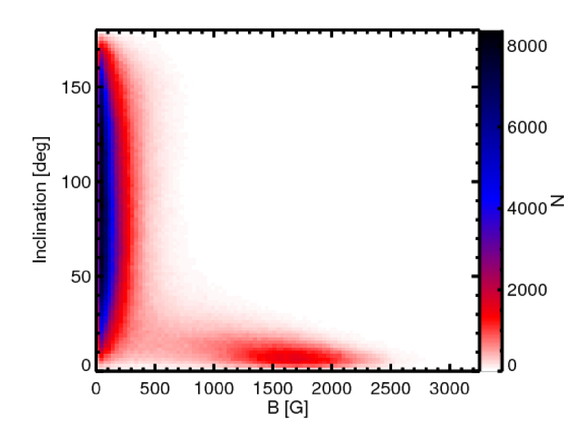
Figure 7: Two-dimensional histogram of the magnetic field strength and inclination of the weak-plage simulation at optical depth unity.

4 Summary and discussion

It has recently been shown that basically all BPs are associated with kilogass fields (Riethmüller et al., 2014). However, it was up to now not so clear which fraction of kiloGauss fields manifests itself in the form of BPs. With the aim of addressing this open question we simulated the upper convection zone and photosphere of the Sun by using the non-gray version of the MURaM code. We calculated ten snapshots each for a mean vertical flux density of 30 G (simulating the quiet Sun), 200 G (weak plage), and 400 G (strong plage), respectively. A full spectral line synthesis in the G-band was then carried out since this spectral range has been frequently used for observations. A typical filter profile was applied to the Stokes $I$ profiles and G-band intensity images were retrieved.

Binned scatter plots of the G-band intensity versus the magnetic field strength (see Fig. 1) displayed a monotonic relation for field strengths higher than about 500 G. The analyses of Röhrbein et al. (2011) and Kahil et al. (2017) showed that the non-monotonic relation with a maximum at intermediate field strength found in scatter plots of observations at continuum wavelengths (e.g., Lawrence et al., 1993; Topka et al., 1997; Kobel et al., 2011; Schnerr & Spruit, 2011) is caused by image smearing due to the limited spatial resolution of observations. Our scatter plot from the weak-plage simulation revealed a similar range in field strength and a considerably larger range in intensity than the simulation carried out by Shelyag et al. (2004), who used an almost identical setup, but with only half of the spatial resolution in the horizontal directions. Horizontal pressure balance leads to an evacuation of strong-field magnetic features and hence to a depression of the optical depth surface. In the theoretical picture of flux tubes used to describe such magnetic features the lateral inflow of radiation through the walls of this depression makes the flux tube hot and bright (Spruit, 1976; Deinzer et al., 1984) with the G-band being particularly sensitive to such brightenings due to the preponderance of CH lines (Sánchez Almeida et al., 2001; Steiner et al., 2001). A doubling in spatial resolution increases in particular the upper limit of the intensity range significantly, which we believe is due to the thinner tube walls produced by the higher resolution which in turn leads to a more effective heating mechanism.

Histograms of the G-band intensity were calculated for pixels exceeding a certain threshold in magnetic field strength. By taking the field strength at the $\tau=1$ surface we excluded pixels in the canopy of magnetic elements. We chose a field strength threshold of 1300 G at $\tau=1$, which corresponds to mainly kiloGauss pixels at $\tau=0.1$, the optical depth to which field strengths retrieved by Milne Eddington inversions roughly refer to. These histograms were then integrated over the intensity starting from a given intensity threshold. This gave us the fraction of strong-field pixels that reached a certain minimum brightness (see Fig. 2). A comparison between such integrated histograms from our simulations of different mean flux densities revealed that kiloGauss magnetic features are on average less bright in plage regions than in the quiet Sun. This is consistent with observations (Solanki & Stenflo, 1984; Solanki, 1986; Lawrence et al., 1993; Ishikawa et al., 2007; Kobel et al., 2011; Romano et al., 2012; Ji et al., 2016) and suggests that at least part of the lower brightness of simulation snapshots having larger magnetic flux (Vögler, 2005) is due to the less bright magnetic features, although a part may be due to the suppression of convection by the magnetic field (e.g., Ishikawa et al., 2007; Kobel et al., 2012; Criscuoli, 2013).

We find that in the quiet Sun the G-band BPs are a very good guide to kiloGauss magnetic fields in that roughly 93% of the area covered by kiloGauss magnetic fields is brighter than average in the G-band (in the absence of spatial smearing and scattered light). This also means that 93% of the kiloGauss flux is captured by G-band BPs. This fraction decreases with increasing magnetic flux, being about 77% for the 200 G weak-plage simulation and just 51% for the 400 G strong-plage simulation. Spatial smearing also decreases the fraction, e.g., for an ideal 0.5 m telescope it goes down to only 78%, 68%, and 41% for the 30 G, 200 G, and 400 G simulation, hence the conclusion of Berger et al. (1995) from their active region observation with a 0.5 m telescope that less than 50% of the small-scale magnetic flux can be identified by visible proxies such as BPs or pores is not in contradiction to the resuls of this study, but can be well explained by the increased mean magnetic flux in the active region and by the limited spatial resolution.

The smaller fraction of bright kiloGauss features in simulations with highest $\langle B_{\rm{z}}\rangle$ has to do with the on average larger magnetic features in such areas. These features are often found to have a slightly dark core in our simulations. The lateral inflow of heat through the walls of a flux tube is balanced by the tube’s radiative losses at the solar surface. With increasing diameter of a flux patch, $d$, the wall area grows with $d$ while the area of radiative losses grows with $d^{2}$. Thus the heating due to the lateral inflow of radiation becomes ineffective for larger flux tubes so that their core becomes dark, while their peripheral regions remain bright (see top panel of Fig. 5). The features we have found to have slightly dark cores are smaller and less dark than pores. They correspond more closely to ’knots’ and ’points’ features found in the older literature (Beckers & Schröter, 1968; Knölker & Schüssler, 1988), or to ’flowers’ and ’micropores’ in more recent publications (Rouppe van der Voort et al., 2005; Narayan & Scharmer, 2010).

During the last few years there has been a debate about the balance between the horizontal and the vertical magnetic flux in the quiet Sun. While some authors find a clear preference for horizontal magnetic fluxes in their observations (e.g., Orozco Suárez et al., 2007; Lites et al., 2008), others claim an isotropic angular distribution of the magnetic field (e.g., Martínez González et al., 2008; Asensio Ramos, 2009), still others find a broad range of field inclinations with a preference of vertical orientations (e.g., Khomenko et al., 2003; Beck & Rezaei, 2009; Borrero et al., 2015, for a review). The fact that the magnetic structuring continues on scales well below the spatial resolution of modern solar telescopes is seen by Stenflo (2010) as the reason for these contradictory results. Stenflo (2010) used quiet-Sun data obtained from Hinode/SP to calculate a scatter plot of the blue lobe Stokes $V$ amplitude derived from the Fe i 630.15 nm line versus the corresponding Stokes $V$ amplitude for the Fe i 630.25 nm line and finds two different magnetic populations.

While the interpretation of the two populations identified by Stenflo (2010) is difficult (in terms of deriving the two relevant physical quantities, magnetic field strength and inclination, from Stokes signals) and still under debate (see Steiner & Rezaei, 2012), we also obtained two different magnetic populations from our analysis, but with a much more straight-forward interpretation, because our MHD data set gives direct access to the relevant physical quantities, is free of noise, and has a much higher spatial resolution. The two-dimensional histograms that we calculated from the magnetic field strength and inclination of our weak-plage simulation shows one population formed exclusively of weak-field pixels displaying a broad range of inclinations. It also shows another population of pixels with mainly strong and more or less vertical fields. A look at the bottom panel of Fig. 5 reveals that all the strong-field pixels lie in the intergranular lanes. The distribution of the inclinations of the weak-field population converges to an isotropic angular distribution at very small flux densities, which was also obtained by Lagg et al. (2016) from their MHD simulations and by Stenflo (2010) from the linear-to-circular polarization ratio of the Hinode/SP data he employed.

The peak field strength of the strong-field population of our weak-plage simulation decreases and the peak inclination weakly increases with atmospheric height, which supports the picture of a thin flux tube expanding with height. From spatially coupled Stokes inversions of Hinode/SP data recorded in a plage region, Buehler et al. (2015) obtained at $\log(\tau)=-0.9$ a typical field strength of 1520 G at inclination angles of $10^{\circ}$-$15^{\circ}$. This agrees well with our results retrieved from the weak-plage simulation at $\log(\tau)=-1$, where we determined the peak of the kiloGauss population to be located at 1400 G and $7^{\circ}$.

Criscuoli & Uitenbroek (2014) used 3D MHD snapshots (calculated with the Stagger code) having a mean magnetic flux density of 200 G and a 22 km cell size in the horizontal direction. They found a bimodal magnetic field distribution for small-scale bright features at an optical depth of $\log(\tau)=-1$. The first peak lay at a field strength close to zero and was caused by bright granules misidentified as BPs and the second peak lay at around 1500 G, which is close to our strong-field peak at that depth, located at 1400 G. Since we used a different MHD code and a spatial resolution twice as high we conclude that this result seems to be relatively insensitive to the details of the simulation.

We mainly considered the question which fraction of the kiloGauss-field regions can be captured by BPs, depending on the spatial resolution and magnetic activity of the observed scene. While in this study we answered this question purely by analyzing MHD simulations, a future study should compare the properties of BPs between simulations and high-resolution active-Sun observations, similar to the study of Riethmüller et al. (2014) for the quiet Sun. A good opportunity might be a combination of active-region observations recorded during the second Sunrise flight (Solanki et al., 2017) and MHD simulations retrieved from these observations via the newly developed MHD-Assisted Stokes Inversion (MASI) technique (Riethmüller et al., 2017) because the new technique provides simulations with a magnetic activity level similar to the observations it matches.