Accelerating Lattice QCD Multigrid on GPUs Using Fine-Grained Parallelization

Abstract

The past decade has witnessed a dramatic acceleration of lattice quantum chromodynamics calculations in nuclear and particle physics. This has been due to both significant progress in accelerating the iterative linear solvers using multi-grid algorithms, and due to the throughput improvements brought by GPUs. Deploying hierarchical algorithms optimally on GPUs is non-trivial owing to the lack of parallelism on the coarse grids, and as such, these advances have not proved multiplicative. Using the QUDA library, we demonstrate that by exposing all sources of parallelism that the underlying stencil problem possesses, and through appropriate mapping of this parallelism to the GPU architecture, we can achieve high efficiency even for the coarsest of grids. Results are presented for the Wilson-Clover discretization, where we demonstrate up to 10x speedup over present state-of-the-art GPU-accelerated methods on Titan. Finally, we look to the future, and consider the software implications of our findings.

1 Introduction

It is well known that continued advances in high performance computing (HPC) have been powered by ever increasing transistor density with each generation, i.e., Moore’s Law. While these advances have continued unabated over the course of 40 years, over the past decade, due to the loss of Dennard scaling, their manifestation has evolved from faster into more parallel. This evolution has had a significant impact on software, since software has had to evolve to enable more parallel processors to be utilized.

Simultaneously, a less-well quantified advance has occurred, that being the one of algorithmic advances: super-linear acceleration of fundamental algorithmic building blocks that underpin computational science. Examples abound from the various disciplines of computational science, e.g., multigrid (MG) [1], Fast Multipole Method [2], Strassen’s matrix multiplication [3], etc. Taken together, the combination of algorithmic and machine advances have revolutionized computational science. Calculations, thought impossible 30 years ago, are now routine. However, this meteoric gain in science throughput is only possible if this combination is multiplicative. Sadly, the recent trends in microprocessor evolution have been divergent with respect to algorithmic advances: the former is becoming ever more parallel, and requires ever more locality (minimization of data movement); in the case of the latter, the critical component of exponential algorithm acceleration is often a serial component, and/or requires non-local communication.

In the present work, we consider the case of lattice quantum chromodynamics (LQCD), a numerically feasible formulation of the theory of the strong force that underpins nuclear and particle physics. This grand challenge application is extremely computationally demanding, often consuming 10%-20% of public supercomputing cycles around the world. While the field has existed for around forty years, it is only recently that both machines and algorithms have advanced enough to bring LQCD predictions to the sub-1% error level, e.g., LQCD calculations are now finally capable of making high-precision predictions for comparison against large-scale accelerator facilities, such as the Large Hadron Collider at CERN.

Graphics processing units (GPUs) have proved to be both a popular and efficient platform on which to build and deploy HPC applications. Present GPUs typically feature thousands of floating point units coupled to a very wide and fast memory bus. GPUs are programmed using a threaded model, utilizing thread oversubscription to hide latency, and require upwards of ten thousand active threads in order to saturate their performance. GPUs are very well suited to LQCD, since these computations feature a lot of trivial data parallelism, as well as having highly-regular memory accesses, which lead to high bandwidth utilization.

One of the largest algorithmic advances in recent years has been the removal of the critical slowing down in the iterative linear solvers that has plagued LQCD computations: as the quark mass parameter is reduced, the condition number of the quark-gluon interaction matrix (known as the Dirac matrix), which must be solved in most LQCD calculations, diverges. This difficulty can be almost completely removed through the use of hierarchical preconditioners such as adaptive MG [4]. The end result is an algorithmic acceleration of the linear solver by potentially upwards of $10\times$. This improved algorithmic scaling will enable larger and more precise computations in the future.

Thus it is obvious to seek the full multiplicative improvement from algorithm and machine. However, GPUs represent an extremely challenging architecture on which to deploy an efficient MG algorithm: the coarse-grid computations that underpin an efficient algorithm are by definition increasingly serial workloads. In this work, using the QUDA library, we demonstrate that through identifying and exposing all of the underlying latent parallelism in the coarse-grid computations we can create a highly efficient MG algorithm implementation. From an LQCD-workload perspective, we focus on the throughput-based workloads of LQCD, that exhibit a lot of task parallelism, and seek to optimize total job throughput. The end result is that we are able to accelerate the analysis workloads by up to $10\times$ over present state-of-the-art LQCD computations on GPUs. In the future, we shall refocus on the other critical workflow in LQCD, gauge generation, which typically uses a Markov-chain Monte Carlo algorithm. In this stage of computation there exists only data parallelism with limited task parallelism, so strong scaling a given problem set is critical for increasing science throughput.

This work is cross cutting since hierarchical algorithms are important for many computational-science disciplines. Moreover, while a given discipline may not be parallelism challenged on current-generation many-core processors, as we trend towards the exascale and beyond, this will be increasingly the case for many fields. Furthermore, we cannot rely on increasing problem set sizes to meet parallelism requirements since in many cases the computational cost grows super-linearly with problem size, so parallelism must be sought elsewhere.

This paper is organized as follows: in $\S$2 we highlight previous work in this area, we give an overview of the LQCD computations we seek to accelerate in $\S$3, and in $\S$4 introduce the QUDA library that underpins this work. We give an overview of our hierarchical framework in $\S$5 and discuss fine-grained parallelization in $\S$6. We show strong-scaling performance curves from the Titan supercomputer in $\S$7; we discuss the software implications in $\S$8 and future research topics in §9 before finally concluding with $\S$10.

2 Previous Work

Lattice QCD calculations on GPUs were originally reported in [5] where the immaturity of using GPUs for general purpose computation necessitated the use of graphics APIs. Since the advent of CUDA in 2007, there has been rapid uptake by the LQCD community. Notable publications include multi-GPU parallelization [6, 7, 8], use of additive Schwarz preconditioning to improve strong scaling [9], software-managed cache-blocking strategies [10], and JIT-compilation to enable the offload of the entire underlying data-parallel framework of the Chroma [11] code without any top-level changes [12]. This work concerns the QUDA library [13], of which we give an overview in §4.

The basic principle of gauge-invariant MG for LQCD was begun with Projective MG in the early 1990s [14]. However only with the advent of an adaptive MG algorithm introduced recently into LQCD [15, 4] was critical slowing down removed completely in the limit of zero quark mass. In parallel, the related approach of Inexact Deflation was introduced [16]; the essential difference between these approaches being that the former utilizes a multiplicative coarse-grid correction, while the latter uses an additive correction. Evolutions of the algorithm introduced include combining it with red-black (or even-odd in LQCD parlance) preconditioning [17] and improving the strong scaling through utilizing a Schwarz-preconditioned domain-decomposition smoother to reduce inter-node communication [18, 19]. These publications have all utilized more traditional CPU-based clusters. Implementations for Intel Xeon Phi Knights Corner have been reported in [20, 21]. To the best of our knowledge there have been no publications concerning the efficient deployment of these MG algorithms for LQCD on GPUs.

The successful deployment of geometric MG on GPUs has been shown in porting the HPGMG benchmark to GPUs [22].

3 Lattice Quantum Chromodynamics

Weakly coupled field theories such as quantum electrodynamics can by handled with perturbation theory. In QCD, however, at low energies perturbative expansions fail and a non-perturbative method is required. LQCD is the only known, model independent, non-perturbative tool currently available to perform QCD calculations.

LQCD calculations are typically Monte-Carlo evaluations of Euclidean-time path integrals. A sequence of configurations of the gauge fields is generated in a process known as configuration generation. The gauge configurations are importance-sampled with respect to the lattice action and represent a snapshot of the QCD vacuum. Configuration generation is inherently sequential as one configuration is generated from the previous one using a stochastic evolution process. As the lattice structure admits data parallelism, many variables can be updated simultaneously, and the focused power of capability computing systems is essential to carry out this phase of the calculations. Once the field configurations have been generated, one moves on to the second stage of the calculation, known as analysis. In this phase, observables of interest are evaluated on the gauge configurations in the ensemble, and the results are then averaged appropriately, to form ensemble averaged quantities. It is from the latter that physical results such as particle energy spectra can be extracted. The analysis phase can be task parallelized over the available configurations in an ensemble and is thus extremely suitable for capacity-level work on clusters, and large ensemble calculations can also make highly effective use of capability-sized partitions of leadership supercomputers. It is the analysis phase that we focus upon in this work.

3.1 Dirac PDE discretization

The fundamental interactions of QCD, those taking place between quarks and gluons, are encoded in the quark-gluon interaction differential operator known as the Dirac operator. As is common in PDE solvers, the derivatives are replaced by finite differences. Thus on the lattice, the Dirac operator becomes a large sparse matrix, $M$, and the calculation of quark physics is essentially reduced to many solutions of systems of linear equations given by

$$Mx=b.$$ (1)

Computationally, the brunt of the numerical work in LQCD for both the gauge generation and analysis phases involves solving such linear systems.

A small handful of discretizations of the continuum operator are in common use, differing in their theoretical properties. Here we focus on the widely-used Sheikholeslami-Wohlert [23] form for $M$, colloquially known as the Wilson-Clover, or simply just Clover discretization.

3.2 Wilson-Clover matrix

The Wilson-Clover matrix is a central-difference discretization of the Dirac operator, with the addition of a diagonally-scaled Laplacian to remove the infamous fermion doublers (which arise due to the red-black instability of the central-difference approximation). When acting in a vector space that is the tensor product of a four-dimensional discretized Euclidean spacetime, spin space, and color space it is given by

$$M_{x,x^{\prime}} =-\frac{1}{2}\displaystyle\sum_{\mu=1}^{4}\bigl{(}P^{-\mu}\otimes U_{x}^{\mu}\,\delta_{x+\hat{\mu},x^{\prime}}\,+P^{+\mu}\otimes U_{x-\hat{\mu}}^{\mu\dagger}\,\delta_{x-\hat{\mu},x^{\prime}}\bigr{)}$$

$$\quad\,+(4+m+A_{x})\delta_{x,x^{\prime}}$$ (2)

Here $\delta_{x,y}$ is the Kronecker delta; $P^{\pm\mu}$ are $4\times 4$ matrix projectors in spin space; $U$ is the QCD gauge field which is a field of special unitary $3\times 3$ (i.e., SU(3)) matrices acting in color space that are ascribed to the links between the spacetime sites (and hence are referred to as link matrices); $A_{x}$ is the $12\times 12$ Clover matrix field acting in both spin and color space,

corresponding to a first-order discretization correction; and $m$ is the quark-mass parameter. The indices $x$ and $x^{\prime}$ are spacetime indices (the spin and color indices have been suppressed for brevity). This matrix acts on a vector consisting of a complex-valued 12-component color-spinor (or just spinor) for each point in spacetime. We refer to the complete lattice vector as a spinor field.

Figure 1: The nearest-neighbor stencil part of the lattice Dirac operator, as defined in (2), in the $\mu-\nu$ plane. The color-spinor fields are located on the sites. The SU(3) color matrices $U^{\mu}_{x}$ are associated with the links.

3.3 Krylov solvers

Iterative Krylov solvers are typically used to obtain solutions to Equation (1), requiring many repeated evaluations of the sparse matrix-vector product. The Wilson-Clover matrix is non-Hermitian, so either Conjugate Gradients [24] on the normal equations (CGNE or CGNR) is used, or more commonly, the system is solved directly using a non-symmetric method, e.g., BiCGStab [25]. Red-black preconditioning is almost always used to accelerate the solution finding process for this system, where the nearest-neighbor property of the $M$ matrix is exploited to solve the Schur complement system [26].

The quark mass controls the condition number of the matrix, and hence the convergence of such iterative solvers. Unfortunately, physical quark masses correspond to highly singular matrices. Given that current lattice volumes are up to $10^{10}$ degrees of freedom, this represents an extremely computationally demanding task. For virtually all LQCD computations, the linear solver accounts for 80–99% of the execution time. Without resorting to eigenvalue deflation or hierarchical approaches, the use of mixed-precision BiCGStab combined with red-black preconditioning represents the state of the art.

3.4 Adaptive Geometric Multigrid

The problem of critical slowing down with the quark mass was long a source of consternation with LQCD computations. While the problem can be alleviated with eigenvector-deflation algorithms, these algorithms scale quadratically with the volume owing to the spectral density scaling approximately linearly with volume, as well as the number of operations scaling linearly with volume. The scalable solution (with respect to problem size) to critical slowing down is the use of adaptive MG.

The scope of this paper is too narrow to permit a careful treatment of the adaptive geometric algorithm deployed for LQCD, so we focus on describing the key parts of the algorithm. As with standard MG, the two critical ingredients to a convergent algorithm are:

• A smoother that effectively reduces high-frequency error components.

• Prolongation and restriction operators that define a coarse grid that captures the near null-space components of the fine-grid linear operator.

What complicates the LQCD case is that the near-null space modes of the Dirac operator (equation 2) are highly oscillatory due to the underlying dependence on the stochastic gauge field, and are not captured by a conventional geometric MG method. The coefficients of the prolongator must therefore be set adaptively to capture this null space by using vectors that are rich in the low-frequency error components of the Dirac operator. Critical to the success of this method is the weak-approximation property of the null space: while eigenvectors are globally (bi-)orthogonal, locally they are co-linear; meaning that a small collection of near-null-space vectors, when partitioned into disjoint local subsets (or aggregates), form a basis that spans the majority of the near-kernel subspace of the operator [27]. Given that the problem is discretized on a homogeneous hypercube, there is no need to use algebraic aggregation, and thus the shape of the aggregates are regular non-overlapping hypercubes. Hence the algorithm is both adaptive and geometric.

The adaptive geometric MG setup is as follows

1. Iterate the homogenous system $Mx=0$ with a random initial guess $x_{0}$. After $k$ iterations the resulting error vector $e_{k}=-x_{k}$ will be rich in slow-to-converge eigenmodes of the operator $M$.

2. Repeat 1) until we obtain enough candidate vectors to capture the near-null space of the operator $M$.

3. Partition the set of null-space vectors $v$ into disjoint aggregates, and perform a QR decomposition on these blocks to form a local orthonormal basis. This forms the columns of the prolongation operator $P$.

4. Compute the resulting coarse-grid operator from the Galerkin product $\hat{M}=P^{\dagger}MP$.

By virtue of the fact that the original fine-grid operator is nearest neighbor only, the coarse-grid operator retains this property. However, due to the aggregation summing over spin and color components of the null-space vectors, the simple tensor-product structure between spin and color spaces on the fine grid is lost on the coarse grid. This manifests itself as a loss in sparsity: the link matrices that exist between lattice sites are of size $\hat{N}_{s}\hat{N}_{c}\times\hat{N}_{s}\hat{N}_{c}$, where $\hat{N}_{c}$ is the number of null-space vectors used to represent the fine-grid null space; this corresponds to the effective number of colors on the coarse grid; $\hat{N}_{s}=2$ is the number of spin degrees of freedom on the coarse grid. The resulting coarse-grid operator takes the form,

$$\hat{M}_{x,x^{\prime}}=-\sum_{\mu}^{4}\left[Y^{-\mu}_{x}\delta_{x+\hat{\mu},x^{\prime}}+Y^{+\mu\dagger}_{x-\hat{\mu}}\delta_{x-\hat{\mu},x^{\prime}}\right]-\delta_{x,x^{\prime}},$$ (3)

where the matrix field $Y$ is the coarse link field.

Aggregates of size $2^{4}-8^{4}$ are usually chosen, with 20-30 vectors required to capture enough of the null-space. The algorithm is recursive, and the setup process can be repeated for an arbitrary number of levels; the coarse-grid operator retains the form in Equation 3 upon subsequent coarsening.

4 The QUDA Library

QUDA (QCD on CUDA) is a library that aims to accelerate LQCD computations through offload of the most time-consuming components of an LQCD application to NVIDIA GPUs. It is a package of optimized CUDA C++ kernels and wrapper code, providing a variety of optimized linear solvers, as well as other performance critical routines required for LQCD calculations. All algorithms can be run distributed on a cluster of GPUs, using MPI to facilitate inter-GPU communication. It has been designed to be easy to interface to existing code bases, and in this work we exploit this interface to use the popular LQCD application Chroma [11]. The QUDA library has attracted a diverse developer community and is being used in production at U.S. national laboratories, as well as in locations in Europe and India. The latest development version is always available in a publically-accessible source code repository [28].

The general strategy is to assign a single GPU thread to each lattice site. Each thread is then responsible for all memory traffic and operations required to update that site on the lattice given the stencil operator. Since the computation always takes place on a regular grid, a matrix-free approach is always used, with the thread coordinate index computed dynamically (see for example Listing 2). Maximum memory bandwidth is obtained by reordering the spinor and gauge fields to achieve memory coalescing, e.g., using structures of float2 or float4 arrays, and using the texture cache where appropriate. Memory-traffic reduction is employed where possible to overcome the relatively low arithmetic intensity of the Dirac matrix-vector operations, which would otherwise limit performance. Strategies include: (a) using compression for the $SU(3)$ gauge matrices to reduce the 18 real numbers to 12 (or 8) real numbers at the expense of extra computation; (b) using similarity transforms to increase the sparsity of the Dirac matrices; (c) utilizing a custom 16-bit fixed-point storage format (hereon referred to as half precision) together with mixed-precision linear solvers to achieve high speed with no loss in accuracy [13].

The library has been designed to allow for maximum flexibility with respect to algorithm parameter space and maximum performance. For example, all lattice objects (fields) maintain their own precision and data ordering as a dynamic variable. This allows for run-time policy tuning of algorithms; these parameters are then bound at kernel launch time when the appropriate C++ template is instantiated corresponding to these parameters. While this flexibility does provide maximum performance it does come at the expense of library binary size.

Key to achieving high performance is the use of auto-tuning: all kernel launch parameters (block size, grid size, shared memory size) are auto-tuned upon first call and cached for subsequent reuse. The autotuner can also tune for arbitrary algorithm policy choices outside of kernel launch parameters (see §6.5).

5 Heterogeneous Software Architecture

MG has both highly parallel throughput-limited parts (fine grids) and more serial, latency-limited parts (coarse grids). Simultaneously, we have an architecture that is composed of throughput (GPUs) and latency optimized (CPUs) processors, so it is natural to consider whether mapping the coarse grids onto the CPU is more efficient. Thus, from the outset, the software-design goal was to enable QUDA to run on the complete heterogeneous architecture in the most efficient manner. To this end, much of QUDA was redesigned to abstract the algorithm from the underlying architecture-specific implementation. Algorithms are expressed in terms of generic fields, with no indication at the algorithmic level as to where the computation is to be executed. Similar to the data order or precision, the location of the data is elevated to a run-time object member, and when executing an algorithm on an object, the object’s location is queried, and the architecture-specific code is executed.

While abstracting the execution location from the algorithm makes it simple to write architecture agnostic high-level algorithms, this still leaves the problem of having to maintain two copies of each computational routine. To remove this burden, we utilize the fact that CUDA and CPU kernels can call common functions if those functions have the __device__ __host__ decorators applied to their declaration. In this way we can use a common codepath for the bulk of the computational routines: the GPU kernel declarations being nothing more than stubs that set indices based on the thread id and call the common function with this index parameter; the CPU functions similarly are stubs that contains for loops over the index range (with optional OpenMP parallelization) that call the common function. The data order is abstracted into generic accessor functors, this allows for different data ordering for the CPU and GPU variants, allowing for optimal deployment on both platforms.

Listing 1: Example of how an axpy computation is deployed using a single code path for GPU and CPU.

⬇

template <typename Arg>

__device__ __host__ void axpy(Arg &arg, int i)

{ arg.y(i) += arg.a * arg.x(i); }

template<typename Arg> // GPU code path

__global__ void axpyGPU(Arg arg) {

int i = blockDim.x*blockIdx.x + threadIdx.x;

if (i >= arg.length) return;

axpy(arg,i);

}

template<typename Arg> // CPU code path

void axpyCPU(Arg &arg) {

#pragma omp for

for (int i=0; i<arg.length; i++) axpy(arg,i);

}

Within the context of MG, it is only at the inter-grid interface, i.e., prolongation and restriction, where it makes sense to switch from one architecture to the other since within a grid we have a roughly constant degree of parallelism and workload. Take for example the restrictor, where we have as input a fine-grid field on the GPU, and output a coarse-grid field on the CPU. Given that the data input is far greater than the output, and the relative narrow PCIe connection between GPU and CPU, we compute the restriction on the GPU and copy the result to the CPU. The converse is true for prolongation.

The consideration of when to offload work to the CPU versus doing it on the GPU is one that has no simple answer, since it depends on many factors, including

• Algorithmic parameters: precision, problem size, etc.

• Relative performance of GPUs and CPUs and the ratio of their numbers per node.

• The CPU-GPU connection bandwidth

• Whether parallel work can be overlapped during the execution of this phase

• Network latency differences between the two memory spaces

The optimal strategy on one machine will thus be different from another. These topics are left unexplored in this work, since as shall be shown below we achieve excellent performance maintaining the entire calculation on the GPU. Given that the QUDA hierarchical framework has been designed to facilitate the offload of arbitrary computation to the CPU as a run-time policy decision, in the future we envisage extending the QUDA autotuning framework to tune for computation location as a policy decision.

6 Fine-grained Parallelization

Prior to this work, all algorithms in QUDA have utilized only the trivial data parallelism over grid points: each thread corresponds to an output grid point, which applies the stencil as a gather operation. This mapping works well for large grids, where large means we have enough grid points, and thus threads, to hide the GPU instruction and memory latencies. Typically this means O(10,000) grid points or greater. In other application domains, coarser-grained parallelizations are possible and may prove optimal if there is sufficient instruction-level parallelism (ILP) to hide latency [29, 30].

For our hierarchical problem, where the coarsest grid size will have as few as $2^{4}$ grid points, or 16-way grid parallelism, such an approach will not be suitable for a GPU. Thus it is critical that we expose all sources of parallelism available to us, and ascertain how to optimally map these to the architecture.

Increasing the degree of parallelization is also important for load balancing. We seek an algorithm that is scalable to an arbitrary number of processing cores, and do not want to rely on a specific core count or vector width. Thus, it is critical that we have a sea of lightweight threads that scale without load balancing or edge effects being apparent.

In the analysis that follows we focus on the coarse-grid operator. Similar analysis applies to the prolongator and restrictor, the specifics of these are covered in §6.6.

6.1 Grid Parallelization

As noted previously, grid parallelism is the trivial data parallelism that arises from assigning one thread per lattice site. There are no inter-thread dependencies, and so the parallelization is trivial. The one dimensional global thread index is trivially mapped to the lattice-site index as shown below. This necessarily involves integer division which adds a non-trivial overhead, however, this is amortized in general when using a coarse-grained decomposition.

Listing 2: Example of how the thread index maps to the lattice coordinates

⬇

// X[] holds the local lattice dimension

int idx = blockIdx.x*blockDim.x + threadIdx.x;

int tmp1 = idx / X[0];

int tmp2 = tmp1 / X[1];

x[0] = idx - tmp1 * X[0];

x[1] = tmp1 - tmp2 * X[1];

x[3] = tmp2 / X[2];

x[2] = tmp2 - x[3] * X[2];

// x[] now holds the thread coordinates

6.2 Color and Spin Parallelization

If we consider Equation 3, the output per site is a color-spinor vector. Each element of this vector is independent, and so like the grid points we can trivially split the computation between threads. Thus we potentially have up to $\hat{N}_{s}\times\hat{N}_{c}$-way additional parallelism that can be exploited. In general we have found using the maximal fine-grained decomposition to be optimal, with each thread computing a single dot product of the matrix-vector multiplication (i.e., one color and spin per thread). We utilize the y-dimension of the CUDA thread index to map to which output element we are computing. In order to optimize between the temporal locality over the y-thread dimension (the input vector is common between threads) versus the need to spread the computation in order to improve load balancing across the GPU the block size in the y dimension is autotuned.

Listing 3: Example of how the y-thread index maps to resulting color-spin indices

⬇

// Nc is the total number of colors

// Mc is the number of colors per thread

int yIdx = blockDim.y*blockIdx.y + threadIdx.y;

int s = yIdx / (Nc/Mc);

int color_subset = (yIdx % (Nc/Mc)) * Mc;

6.3 Stencil Direction Parallelization

The next level of parallelism we can exploit is that provided by the stencil direction: the $\mu$ index from Equation 3 as well as the forwards and backwards directions. This provides up to an additional eight-way parallelism, however, we must sum the partial results before writing to main memory. In CUDA this is easily done by ensuring that all threads responsible for a given output element are assigned with the same thread block:

1. Each thread computes its contribution to the sum.

2. Each thread writes its result to shared memory.

3. Synchronize the thread block.

4. Threads responsible for, say, $\mu=0$ and forwards direction, sum all results from shared memory and writes to global memory.

Parallelization over the stencil direction is mapped to the z-thread dimension, with the mapping $\mu*2+dir$ being a trivial variation of Listing 3. On larger grids it was found to be detrimental to parallelize the stencil direction, and the optimal degree of splitting varies across GPU architecture. Thus, the degree to which the stencil is parallelized is a templated parameter, and the autotuner ascertains the optimal splitting for a given problem size and architecture.

6.4 Dot Product Parallelization

Since the grid sites are assigned the fastest varying thread index (x dimension), on the smallest grids, e.g., $V=2^{4}$, we will not have enough grid sites to fill a warp and guarantee full SIMD efficiency, since warp threads could diverge. To remedy this, we can partition the dot-product computation that corresponds to multiplying a row of the link-matrix by a site vector. In general, such dot products are unsuitable for parallelizing since they are tightly coupled and combining the results from individual dot products would require costly synchronization. However, here we only seek to expose enough parallelism to enable us to fill the warp, e.g., 2-way splitting of the dot product for 16 grid points. To do so, we utilize the warp-shuffle instruction that allows for low-latency communication between threads in the same warp without the need to synchronize.

Listing 4: Example $N$-way dot product partitioning using the warp shuffle instruction to maximize thread efficiency

⬇

const int warp_size = 32; // warp size

const int n_split = 4; // four-way warp split

const int grid_pts = warp_size / n_split;

complex<real> sum = 0.0;

for (int i=0; i<N; i+=n_split)

sum += a[i] * b[i];

// cascading reduction

for (int offset = warp_size/2; offset >= grid_pts; offset /= 2)

sum += __shfl_down(sum, offset);

// first grid_pts threads now hold result

Finally, we expose ILP, allowing for intra-thread latency hiding. This optimization is more important for the Kepler architecture that Titan features, since it has higher dependent instruction latency (nine clock cycles) than the more recent Maxwell and Pascal (six clock cycles).

Listing 5: Example of how ILP is exploited to increase throughput for an $N$-way complex dot-product type computation

⬇

const int n_ilp = 2; // two-way ILP

complex<real> sum[n_ilp] = { };

for (int i=0; i<N; i+=n_ilp)

for (int j=0; j<n_ilp; j++)

sum[j] += a[i+j] * b[i+j];

complex<real> total = static_cast<real>(0.0);

for (int j=0; j<n_ilp; j++) total += sum[j];

6.5 Performance

Figure 2: Single-precision performance of the coarse-grid operator as a function of decreasing lattice size for 24 and 32 colors (Tesla K20X, CUDA 7.5, GCC 4.9).

In Figure 2 we show the performance of the coarse operator as a function of decreasing lattice size, with each strategy being cumulative with previous ones. The Tesla K20X used here matches that of the Titan used in our final result in §7. Given that the arithmetic intensity (in FP32) of the coarse operator is close to unity, 140 GFLOPS represents around 80% of achievable STREAM bandwidth, and so represents a reasonable performance upper bound. In comparison, the Wilson-Clover operator sustains $\sim 400$ GFLOPS on equivalent fine-grid size. The former is much smaller than the latter due to the decreased temporal locality arising from the loss in tensor structure. For all but the smallest lattice size, the addition of color-spin parallelization is enough to saturate performance. On the $2^{4}$ lattice, all sources of parallelism are necessary, and even then performance is not saturated. Profiling revealed this to be due to the fixed indexing cost that represents the Amdahl’s law limiter, e.g., Listing 2. We note that on the $2^{4}$ lattice with 32 colors, the fine-grained parallelization results in 32768-way parallelism, instead of the naïve 16-way parallelism, and resulted in a 100x speedup. Future optimization in this area could focus on optimization of the indexing overhead, e.g., through computing the integer division magic numbers on the host prior to launching the coarse-grid kernel [32].

In deploying the coarse-grid operator on multiple nodes, halo packing and exchange routines are needed as well. To achieve good bandwidth saturation on the packing kernel, a fine-grained parallelization strategy over site, color and spin was deployed. Given that halo exchange is $O(\hat{N}_{s}\hat{N}_{c})$ but stencil application is $O(\hat{N}_{s}^{2}\hat{N}_{c}^{2})$ the halo-exchange cost is relatively negligible. Thus we focussed on minimizing latency of the communication: a single packing kernel is used for all exchange dimensions followed by a single copy to the CPU of the resulting buffer. MPI is used to exchange the halos and a subsequent single copy to the GPU is utilized. In this initial implementation overlapping of computation and communication is not performed (unlike on the fine grid which is optimized for throughput).

6.6 Inter-grid Transfer Operators

The transfer operators (prolongator and restrictor) are special since they involve both fine and coarse grids. To maximize parallelism we always parallelize with respect to the fine-grid geometry. For the prolongator this is trivial, since the output is on the fine grid, so it can be implemented as a gather operation, and we can easily assign independent threads to each fine-grid degree of freedom (grid, color, spin). The restrictor is not so simple, since here the input is a fine-grid field, and trivial parallelism over the fine-grid degrees of freedom would imply a scatter operation (onto the coarse grid), requiring atomics to avoid a race between threads. The solution is twofold: we parallelize over the output (coarse) color and spin, and parallelize over the input grid geometry. To avoid a race condition on the latter we ensure that a single aggregate (for a given coarse color and spin) is always mapped exactly to a thread block: each thread then performs the necessary rotation from fine degrees of freedom (color and spin) to coarse degrees of freedom, and then a shared-memory reduction obtains the final coarse-grid result, with the first thread in the thread block writing out the final coarse-grid result. For rapid development, as well as high performance, we utilized the cub C++ header library for this [33].

6.7 Summary

In this section we have described how the many sources of parallelism in a stencil problem can be exposed and mapped to the GPU architecture. Critical in achieving this mapping in a flexible fashion is the scalar SIMT programming model that GPUs feature, utilizing a hierarchical Cartesian grid for expressing locality, as well as the low-latency shared-memory that clusters of threads can utilize as a common scratchpad to share data. These features enable us to extract enough parallelism to saturate the GPU on all but the smallest problem sizes.

Due to the achieved high saturation of GPU performance, we have not pursued an optimized CPU coarse-grid implementation beyond rudimentary OpenMP parallelization. We discuss our long-term expectations with respect to CPU versus GPU for the coarse-grid computation in §9.

7 Results

7.1 Methodology

All the results for this section were carried out on the Titan System, hosted at Oak Ridge Leadership Computing Facility (OLCF). We used a development version of QUDA and Chroma. The codes were compiled using the GNU C/C++ compiler (gcc) v4.9.0, and CUDA-toolkit version 7.0 as installed on Titan. We carried out solves with the MG solver in QUDA, and compared performance with QUDA’s mixed-precision BiCGStab algorithm.

We selected three exemplar gauge configurations for this study that are representative of present LQCD computations on Leadership facilities, the parameters of which we list in Table 1: $L_{s}$ and $L_{t}$ refer to the number of lattice sites in the 3 spatial and the temporal direction respectively; the lattice spacings $a_{s}$ and $a_{t}$ refer to the lattice spacings in femtometers, $m_{q}$ is the bare sea quark mass parameter used for the light quarks in the configuration generation, and $m_{\pi}$ gives the mass of the $\pi$-meson measured on the lattices to indicate the lightness of the sea quarks.

In our studies the solves were carried out with the quark mass parameter equal to the sea quark masses on these configurations.

Table 1: Lattice configurations and their physical parameters

Label	$L_{s}$	$L_{t}$	$a_{s}$(fm)	$a_{t}$ (fm)	$m_{q}$	$m_{\pi}$ (MeV)
Aniso40	$40$	$256$	$0.125$	$0.035$	$-0.0860$	$\approx 230$
Iso48	$48$	$96$	$0.075$	$0.075$	$-0.2416$	$\approx 192$
Iso64	$64$	$128$	$0.075$	$0.075$	$-0.2416$	$\approx 192$

On each configuration we computed a “propagator”, which consists of 12 independent linear solves, and compared the time to solution between MG and BiCGStab. Since in the first solve QUDA performs performance autotuning, the wallclock time for these was artificially long, and so in our results we have averaged the wallclock times on the last 11 solves following this. For computing the lattice-averaged quantities (e.g., residual) we use the $L_{2}$ norm, and estimate the solver error using the double-solve strategy advocated in [17]. For speedups we take the ratio of wallclock times and averaging the ratios: in other words, the solves are treated as though they are correlated. We do not include the MG set-up time because in a throughput calculation this time is completely amortized by a very large number of solves. For example in hadron spectroscopy calculations $O(10^{5})-O(10^{6})$ solves may be carried out per gauge configuration. Optimizing the setup both algorithmically and in terms of implementation is beyond the scope of our discussion here but will be covered in future work.

For MG, we used a three-level K-cycle: on the fine and intermediate levels we used a recursively preconditioned general conjugate residual (GCR) algorithm with a Krylov subspace size of 10 vectors. For smoothing on these levels four pre and post applications of minimal residual (MR) was used and the coarse-grid solver was GCR. GCR was chosen as the outer solver since it is a flexible solver, thus is tolerant of the variable precondioner that arises from using an MR smoother in a K-cycle. On all levels we utilized red-black preconditioning. On the finest level, in the MR smoother we used half precision, and we compressed the gauge field to eight real numbers. With the exception of using double precision on the outer most GCR solver, all other computation was in single precision. The BiCGStab algorithm employed half precision with double-precision reliable updates and similarly utilized gauge compression.

In our tests, we investigated three MG sub-space size combinations: a) 24 null vectors on both level 1 and level 2, b) 24 null vectors on level 1, 32 null vectors on level 2 and c) 32 null vectors on both level 1 and level 2. These representing typical choices in a CPU MG method. We refer to these strategies as $24/24$, $24/32$ and $32/32$ respectively.

Given our interest in the analysis phase of LQCD for the Aniso40 and Iso48 data we have only investigated small partiton sizes of 20 and 32 nodes for Aniso40 and 24 and 48 nodes for Iso48 respectively (note for Aniso40, the $32/32$ case did not fit on 20 nodes). For the Iso64 dataset we found the minimum partition size to be 64 nodes, and since the lattices are relatively large, we scaled this out to 512 nodes. Our current implementation cannot scale beyond this node count, since in this case the size of the coarsest lattice is $2^{4}$ sites per node, which is the minimum our implementation can handle.

Table 2: Chief parameters for the MG tests.

Label	Nodes	Level 1	Level 2	target
		blocking	blocking	residuum
Aniso40	$20$	$5^{2}\times 2\times 8$	$2^{3}\times 4$	$5\times 10^{-6}$
Aniso40	$32$	$5^{3}\times 8$	$2^{3}\times 4$	$5\times 10^{-6}$
Iso 48	$24,48$	$4^{4}$	$3^{3}\times 2$	$10^{-7}$
Iso 64	$64,128,256,512$	$4^{4}$	$2^{4}$	$10^{-7}$

7.2 Scaling Results

Table 3: Results Table. Mean values are shown with standard deviation in brackets.

		BiCGStab				Multigrid
Label	Nodes	Iter.	Time(s)	Error/	Nodes	Strategy	Iter.	Time(s)	Error/	Nodes	Speedup
				Residual	$\times$ Time				Residual	$\times$ Time
Aniso40	20	1771 (86)	22.6 (1.9)	137 (38)	452	24/24	15.3 (0.5)	2.9 (0.1)	42.9 (2.2)	58.0	7.7 (0.6)
						24/32	14.2 (0.4)	2.9 (0.1)	30.2 (1.2)	58.0	7.9 (0.7)
	32	1817 (139)	11.8 (0.9)	134 (42)	338	24/24	17.6 (0.5)	2.01 (0.04)	36.6 (7.2)	64.3	5.5 (1.2)
						24/32	17.9 (0.3)	1.95 (0.07)	43.8 (2.2)	62.4	6.0 (0.5)
						32/32	14.0 (0.0)	2.09 (0.03)	26.1 (1.2)	66.9	5.6 (0.5)
Iso48	24	3402 (132)	20.4 (1.3)	110 (33)	490	24/24	17.4 (0.5)	3.84 (0.13)	24.9 (1.8)	92.2	5.3 (0.2)
						24/32	17.3 (0.5)	3.12 (0.10)	26.8 (4.5)	74.9	6.6 (0.5)
						32/32	14.0 (0.0)	4.16 (0.13)	25.1 (4.5)	99.8	5.1 (0.4)
	48	3522 (245)	14.4 (1.0)	99.8 (29.2)	691	24/24	17.2 (0.4)	2.23 (0.05)	25.6 (2.1)	107	6.3 (0.4)
						24/32	17.0 (0.0)	2.36 (0.07)	25.1 (2.0)	113	6.1 (0.4)
						32/32	14.0 (0.0)	2.84 (0.07)	25.9 (2.0)	136	5.1 (0.4)
Iso64	64	2805 (159)	22.2 (1.7)	210 (84)	1421	24/24	17.4 (0.5)	4.11 (0.15)	29.9 (2.3)	263	5.4 (0.4)
						24/32	17.0 (0.0)	4.48 (0.96)	25.7 (1.7)	287	5.1 (0.8)
						32/32	14.0 (0.0)	4.63 (0.15)	31.4 (7.4)	296	4.8 (0.3)
	128	2807 (171)	30.7 (2.4)	199 (90)	3930	24/24	18.0 (0.0)	3.01 (0.06)	33.6 (1.5)	385	10.2 (0.7)
						24/32	16.7 (0.5)	3.05 (0.07)	24.7 (1.8)	390	10.1 (0.6)
						32/32	14.0 (0.0)	3.46 (0.05)	31.8 (9.3)	443	8.9 (0.6)
	256	2885 (171)	22.5 (1.8)	191 (76)	5760	24/24	18.0 (0.0)	2.36 (0.07)	32.0 (4.1)	604	9.5 (0.8)
						24/32	16.4 (0.5)	2.12 (0.08)	24.5 (2.0)	543	10.6 (0.8)
						32/32	14.0 (0.0)	2.37 (0.06)	32.1 (5.3)	607	9.5 (0.7)
	512	2940 (269)	12.3 (0.7)	198 (80)	6298	24/24	17.9 (0.3)	1.73 (0.08)	33.2 (2.0)	886	7.1 (0.4)
						24/32	17.0 (0.0)	1.97 (0.10)	25.8 (2.0)	1009	6.3 (0.3)
						32/32	13.7 (0.5)	1.93 (0.13)	33.4 (5.8)	988	6.4 (0.2)

Our results are given in Table 3, where we compare the iteration count, average wallclock time, error/residual ratio and cost (defined as number of nodes $\times$ time) for the solvers, as well as the MG wallclock speedup versus BiCGStab at constant node count. Figure 3 is a visual repsentation of these wallclock times. One of the propagator solves on the $24/24$ case took anomalously long: we have excluded this, together with the corresponding solves from the $24/32$, $32/32$ and BiCGStab results. Likewise, we found an anomalously large value for MG with $24/32$ for the Iso64 workload; we again treated it as an anomaly and excluded that component from the analysis for all the solver setups. These exclusions did not change the average values significantly, but rather changed the error bars which were otherwise excessively large. Our experience has been that such fluctations are commonplace when running on Titan and we hypothesis are due to cross-job network polution.

In going from 64 nodes to 128 nodes the BiCGStab runtime increases, rather than decreases, though for partitions larger than 128 nodes BiCGStab runtime scales reasonably. This observation was repeatable and does not occur with MG. We attribute this to node placement for the job, possibly due to having the job fit into one cabinet on 64 nodes, to no longer fitting into one cabinet for 128 nodes. Moreover, BiCGStab is more strictly communications limited compared to MG’s more latency-limited profile.

The speedup of MG over BiCGStab is typically between 5–8$\times$, although it exceeds $10\times$ in the case of the Iso64 dataset on 128 and 256 nodes. In all cases the minimum cost occurs on the least numbers of nodes, demontrating the difficulty in strong scaling sparse iterative solvers. In most cases the 24/24 and 24/32 strategies proved to be superior; while 32/32 gives a better preconditioner since it captures more of the null space, the increased cost of the intermediate grid results in a net computational loss.

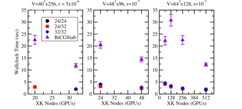
Figure 3: MG scaling vs BiCGStab for the datasets given in Table 1, algorithm parameters given in 2 and §7.1.

The drastically reduced and stable iteration count of MG demonstrates its numerical robustness compared to the more chaotic convergence of BiCGStab. The reduced error / residual ratio is indicative of MG’s ability to damp both the high and low error modes uniformly: thus the cost reduction at constant error will be even greater than the naïve speedups shown in Table 3.

We do not focus on raw GFLOPS rates here, but we note that MG typically sustains around 3–5$\times$ less GFLOPS than BiCGStab when running on the same number of GPUs. Using the nvidia-smi utility we compared the power efficiency of the two algorithms: typically MG consumes $\sim 15\%$ less power than BiCGStab, e.g., for Iso48 on 48 nodes, node 0 used 72W for MG versus 83W for BiCGStab. This is not surprising given the reduced GFLOPS performance of MG versus BiCGStab; hence MG is also more power efficient as well as more time efficient.

To better understand the rate-limiting step of the MG solver, in Figure 4 we show the breakdown of time spent in three different levels of the solver for the large Iso64 problem as a function of the number of nodes. It can be seen that the coarsest grid constitutes an ever increasing fraction of the time spent. Closer profiling revealed this to be due to the global synchronizations present in the coarse-grid GCR solver: the $\log N$ scaling of the cost of synchronization dominates that of the stencil application at large node count.

Figure 4: Breakdown of time spent in the different MG levels for the Iso64 dataset with the 24/32 strategy.

8 Software Implications of Fine-grained Parallelization

As noted in §6, the most commonly deployed approach to parallelizing grid-based stencil computation is to employ the data parallelism of the underlying grid. In LQCD this approach is particularly attractive, since it means that the underlying physics can be expressed in terms of the natural matrices, vectors, etc. that underpin these theories. It is exactly this strategy that domain-specific languages (DSLs) have employed in LQCD: large code bases have been built on this principle, e.g., Chroma, the newly introduced Grid framework [34], etc. With this data-parallel abstraction, it is then possible to deploy these applications on a variety of architectures in a portable fashion. However, by expressing computation at the grid level, this excludes the kind of fine-grained parallelization strategies employed in this work. With a hierarchy of scales, MG certainly exaggerates the need for this in today’s architecture, however, as we move to ever more parallel systems, the need for fine-grained parallelism will eventually extend in a more intrusive manner into software, e.g., not just in the coarse-grid of a MG solve. Given potential super-linear scaling of algorithmic cost with respect to problem size, we cannot rely upon weak scaling in order to saturate future machines and meet the expected science fidelity goals. In planning for the scalable software models for the Exascale and beyond, we advocate a multi-resolution approach for future frameworks, by which we mean interfaces to work both at the level of grid parallelism or at levels where the extra degrees of parallelism are fully exposed. The majority of the code can then be written in the simpler style as before, but frameworks would be able to also accommodate the parallelism needed for performance critical sections. This statement is not specific to GPUs, e.g., the recent Intel Knights Landing architecture with up to 72 cores, each with wide vectors units and multiple SIMT threads, may well require similar optimization strategies.

9 Future Work

This work focussed on accelerating throughput workloads, but not on the strong scaling workloads. Future work will focus on this area, in particular through the use of Schwarz-style communication-reducing preconditioners to improve strong scaling of the MG smoothers [19, 18], and through replacement of the coarse-grid solver with a latency tolerant solver, such as CA-GMRES [35, 36].

Another avenue to increase parallelism is to reformulate MG as a multiple-right-hand-side solver, where we solve multiple linear systems simultaneously. For $N$ right hand sides, we thus expose $N-$way additional parallelism, as well as increasing the temporal locality of the problem, e.g., the same stencil operator is used for all systems. We see this as another critical reformulation to maintain scalability on future architectures (c.f. [21]).

While at present, GPUs are efficient for the entire MG computation, we expect in the future coarse grids will favor latency-optimized CPUs since throughput-optimized processors (e.g., GPUs) will continue to get wider and at some point exhaust all available parallelism. When this point is reached, as it has been in other MG formulations, e.g., [22], the algorithm will then be optimally deployed on the heterogeneous architecture. It is then tempting to wonder whether we can utilize the CPU and GPU simultaneously using an additive correction at the boundary between architectures. While additive multigrid is known not to extend to multiple levels, in this case we only seek an additive correction at the interface, and maintain a multiplicative correction elsewhere.

10 Conclusions

This report is a step in a critical transition for LQCD, as it explores finer resolution with multiple physical scales and adapts to increasingly parallel architectures on the path to the Exascale. MG is a dramatic example of the huge algorithmic potential of incorporating multiple scales in software infrastructure. Algorithmic gains of one to two orders of magnitude are too compelling and must be accommodated. However, the hyper parallelism of many-core architectures often conflicts with the multi-scale algorithmic needs that require fine-grain parallelism and non-local memory references. We believe this article is a prototypical example of the substantial software restructuring needed to combine multi-scale algorithms with future architectures across many disciplines of computational science.

Already precision results in lattice LQCD are competing in accuracy with the best experimental results. This in turn has established LQCD as a necessary partner with experiment in the fundamental search for new physics beyond the Standard Model at the Large Hardon Collider and at nuclear and particle physics laboratories around the world. For LQCD to continue to advance in this enterprise, further research along the lines in this limited study must proceed in the next decade to maintain the momentum in the exploration of particle and nuclear physics.

Appendix: Reproducibility

The source code of the programs used, the input and output data, run-scripts and post processing scripts used to generate the data in this paper can be made available on request, along with assistance in code-building, installation and running. Please contact B. Joó for details.

References

- [1] A. Brandt, “Multi-level adaptive solutions to boundary-value problems,” Mathematics of Computation, vol. 31, no. 138, pp. 333–390, 1977. [Online]. Available: http://www.jstor.org/stable/2006422
- [2] V. Rokhlin, “Rapid solution of integral equations of classical potential theory,” Journal of Computational Physics, vol. 60, no. 2, pp. 187 – 207, 1985. [Online]. Available: http://www.sciencedirect.com/science/article/pii/0021999185900026
- [3] V. Strassen, “Gaussian elimination is not optimal,” Numerische Mathematik, vol. 13, no. 4, pp. 354–356, 1969. [Online]. Available: http://dx.doi.org/10.1007/BF02165411
- [4] R. Babich et al., “Adaptive multigrid algorithm for the lattice Wilson-Dirac operator,” Phys. Rev. Lett., vol. 105, p. 201602, 2010.
- [5] G. I. Egri, Z. Fodor, C. Hoelbling, S. D. Katz, D. Nógrádi, and K. K. Szabó, “Lattice QCD as a video game,” Computer Physics Communications, vol. 177, no. 8, pp. 631 – 639, 2007.
- [6] R. Babich, M. A. Clark, and B. Joó, “Parallelizing the QUDA Library for Multi-GPU Calculations in Lattice Quantum Chromodynamics,” in Proceedings of the 2010 ACM/IEEE International Conference for High Performance Computing, Networking, Storage and Analysis, ser. SC ’10. Washington, DC, USA: IEEE Computer Society, 2010, pp. 1–11.
- [7] G. Shi, S. Gottlieb, A. Torok, and V. V. Kindratenko, “Design of MILC lattice QCD application for GPU clusters,” in IPDPS. IEEE, 2011.
- [8] A. Alexandru, M. Lujan, C. Pelissier, B. Gamari, and F. X. Lee, “Efficient implementation of the overlap operator on multi- GPUs,” 2011.
- [9] R. Babich, M. A. Clark, B. Joo, G. Shi, R. C. Brower, and S. Gottlieb, “Scaling Lattice QCD beyond 100 GPUs,” in SC11 International Conference for High Performance Computing, Networking, Storage and Analysis Seattle, Washington, November 12-18, 2011, 2011. [Online]. Available: http://inspirehep.net/record/927455/files/arXiv:1109.2935.pdf
- [10] R. Babich and M. A. Clark, “High-efficiency Lattice QCD computations on the Fermi architecture,” ser. Innovative Parallel Computing (InPar), 2012.
- [11] R. G. Edwards and B. Joó, “The Chroma software system for lattice QCD,” Nucl. Phys. Proc. Suppl., vol. 140, p. 832, 2005.
- [12] F. T. Winter, M. A. Clark, R. G. Edwards, and B. Joó, “A Framework for Lattice QCD Calculations on GPUs,” 2014. [Online]. Available: http://inspirehep.net/record/1312379/files/arXiv:1408.5925.pdf
- [13] M. A. Clark, R. Babich, K. Barros, R. C. Brower, and C. Rebbi, “Solving Lattice QCD systems of equations using mixed precision solvers on GPUs,” Comput. Phys. Commun., vol. 181, pp. 1517–1528, 2010.
- [14] R. C. Brower, R. G. Edwards, C. Rebbi, and E. Vicari, “Projective multigrid for Wilson fermions,” Nucl. Phys., vol. B366, pp. 689–705, 1991.
- [15] J. Brannick, R. C. Brower, M. A. Clark, J. C. Osborn, and C. Rebbi, “Adaptive Multigrid Algorithm for Lattice QCD,” Phys. Rev. Lett., vol. 100, p. 041601, 2008.
- [16] M. Lüscher, “Local coherence and deflation of the low quark modes in lattice QCD,” JHEP, vol. 07, p. 081, 2007.
- [17] J. C. Osborn, R. Babich, J. Brannick, R. C. Brower, M. A. Clark, S. D. Cohen, and C. Rebbi, “Multigrid solver for clover fermions,” PoS, vol. LATTICE2010, p. 037, 2010.
- [18] A. Frommer, K. Kahl, S. Krieg, B. Leder, and M. Rottmann, “Adaptive Aggregation Based Domain Decomposition Multigrid for the Lattice Wilson Dirac Operator,” SIAM J. Sci. Comput., vol. 36, pp. A1581–A1608, 2014.
- [19] ——, “An adaptive aggregation based domain decomposition multilevel method for the lattice wilson dirac operator: multilevel results,” 2013.
- [20] S. Heybrock, M. Rottmann, P. Georg, and T. Wettig, “Adaptive algebraic multigrid on SIMD architectures,” in Proceedings, 33rd International Symposium on Lattice Field Theory (Lattice 2015), 2015. [Online]. Available: https://inspirehep.net/record/1409505/files/arXiv:1512.04506.pdf
- [21] D. Richtmann, S. Heybrock, and T. Wettig, “Multiple right-hand-side setup for the DD- AMG,” in Proceedings, 33rd International Symposium on Lattice Field Theory (Lattice 2015), 2016. [Online]. Available: https://inspirehep.net/record/1415122/files/arXiv:1601.03184.pdf
- [22] N. Sakharnykh, “High-Performance Geometric Multi-Grid with GPU Acceleration,” 2016.
- [23] B. Sheikholeslami and R. Wohlert, “Improved Continuum Limit Lattice Action for QCD with Wilson Fermions,” Nucl. Phys., vol. B259, p. 572, 1985.
- [24] M. R. Hestenes and E. Stiefel, “Methods of Conjugate Gradients for Solving Linear Systems,” Journal of Research of the National Bureau of Standards, vol. 49, no. 6, pp. 409–436, Dec. 1952.
- [25] H. A. van der Vorst, “Bi-CGSTAB: A Fast and Smoothly Converging Variant of Bi-CG for the Solution of Nonsymmetric Linear Systems,” SIAM Journal on Scientific and Statistical Computing, vol. 13, no. 2, pp. 631–644, 1992.
- [26] T. A. Degrand and P. Rossi, “Conditioning techniques for dynamical fermions,” Computer Physics Communications, vol. 60, no. 2, pp. 211 – 214, 1990.
- [27] M. Brezina, R. Falgout, S. Maclachlan, T. Manteuffel, S. Mccormick, and J. Ruge, “Adaptive Smoothed Aggregation SA Multigrid,” SIAM Review, vol. 47, no. 2, pp. 317–346, 2005.
- [28] http://lattice.github.com/quda, 2011.
- [29] P. Micikevicius, “3D Finite Difference Computation on GPUs Using CUDA,” in Proceedings of 2Nd Workshop on General Purpose Processing on Graphics Processing Units, ser. GPGPU-2. New York, NY, USA: ACM, 2009, pp. 79–84. [Online]. Available: http://doi.acm.org/10.1145/1513895.1513905
- [30] V. Volkov, “Programming inverse memory hierarchy: case of stencils on GPUs,” 2010.
- [31] B. Catanzaro, “Generics,” https://github.com/bryancatanzaro/generics, 2014.
- [32] M. Milakov, “Fast integer division,” https://github.com/milakov/int_fastdiv, 2015.
- [33] D. Merrill, “CUB,” https://nvlabs.github.io/cub, 2016.
- [34] P. Boyle, A. Yamaguchi, G. Cossu, and A. Portelli, “Grid: A next generation data parallel C++ QCD library,” 2015.
- [35] M. Hoemmen, “Communication-avoiding Krylov Subspace Methods,” Ph.D. dissertation, Berkeley, CA, USA, 2010, aAI3413388.
- [36] S. Williams, M. Lijewski, A. Almgren, B. V. Straalen, E. Carson, N. Knight, and J. Demmel, “s-Step Krylov Subspace Methods as Bottom Solvers for Geometric Multigrid,” in Parallel and Distributed Processing Symposium, 2014 IEEE 28th International, May 2014, pp. 1149–1158.