Spectral algorithms for tensor completion

Abstract.

In the tensor completion problem, one seeks to estimate a low-rank tensor based on a random sample of revealed entries. In terms of the required sample size, earlier work revealed a large gap between estimation with unbounded computational resources (using, for instance, tensor nuclear norm minimization) and polynomial-time algorithms. Among the latter, the best statistical guarantees have been proved, for third-order tensors, using the sixth level of the sum-of-squares (sos) semidefinite programming hierarchy (Barak and Moitra, 2014). However, the sos approach does not scale well to large problem instances. By contrast, spectral methods — based on unfolding or matricizing the tensor — are attractive for their low complexity, but have been believed to require a much larger sample size.

This paper presents two main contributions. First, we propose a new unfolding-based method, which outperforms naive ones for symmetric $k$-th order tensors of rank $r$. For this result we make a study of singular space estimation for partially revealed matrices of large aspect ratio, which may be of independent interest. For third-order tensors, our algorithm matches the sos method in terms of sample size (requiring about $rd^{3/2}$ revealed entries), subject to a worse rank condition ($r\ll d^{3/4}$ rather than $r\ll d^{3/2}$). We complement this result with a different spectral algorithm for third-order tensors in the overcomplete ($r\geq d$) regime. Under a random model, this second approach succeeds in estimating tensors of rank $d\leq r\ll d^{3/2}$ from about $rd^{3/2}$ revealed entries.

1. Introduction

Tensors are increasingly ubiquitous in a variety of statistics and machine learning contexts. Many datasets are arranged according to the values of three or more attributes, giving rise to multi-way tables which can be interpreted as tensors [Mør11]. For instance, consider the collaborative filtering problem in which a group of users provide feedback on the episodes of a certain number of television shows, over an extended time interval. The data is indexed by three attributes — user id, show id, and episode broadcast time — so it is presented as a three-way table (which is a tensor). A second example comes from high-dimensional applications of the moment method [HKZ12]: the $k$-th moments of a multivariate distribution are naturally encoded by a $k$-fold tensor. Some other applications include image inpainting [LMWY13], hyperspectral imaging [LL10, SVdPDMS11], and geophysical imaging [KSS13].

In many applications, the underlying tensor $\bm{T}$ is only partially observed, and it is of interest to use the observed entries to impute the missing ones. This is the tensor completion problem. Clearly, completion is plausible only if the underlying tensor $\bm{T}$ is sufficiently structured: it is standard to posit that it has low rank, and is incoherent with respect to standard basis vectors. These assumptions are formalized in a few non-equivalent ways in the existing literature; we review some of these below. We assume an underlying order-$k$ tensor, $\bm{T}\in(\mathbb{R}^{d})^{\otimes k}$ — it is a $k$-way array, with entries $\bm{T}_{\underline{\smash{u}}}$ indexed by ${\underline{\smash{u}}}\in[d]^{k}$ where $[d]\equiv\{1,\ldots,d\}$. Our basic structural assumption is that $\bm{T}$ has low rank in the sense that it is expressible as a sum of $r$ pure tensors:

$$\bm{T}=\sum_{s\leq r}a^{(1)}_{s}\otimes\cdots\otimes a^{(k)}_{s}\,.$$ (1)

This paper proposes methods for completing $\bm{T}$ from n observed entries, and investigates the minimum number n (as a function of $k,d,r$) required for a non-trivial estimator.

1.1. Related work

There is already a substantial literature on tensor completion, and we survey here some of the main ideas that have emerged.

Non-polynomial estimators

Motivated by the success of methods for matrix completion based on nuclear norm relaxations [CR09, Gro11], several papers have studied estimators based on a suitable definition of tensor nuclear norm [YZ15, YZ16]. This tensor norm is np-hard to evaluate [FL16] and therefore this approach does not lead to practical algorithms. Nevertheless these studies provide useful information on the minimum number n of entries required to reconstruct $\bm{T}$ with unbounded computational resources. In particular, it was proved [YZ16] that it suffices to have

$$\textsf{n}\geq\textsf{C}d(\log d)^{2}\max\bigg{\{}(r_{\textup{\tiny$\boxplus$},\mbox{\tiny\rm max}})^{k-1},(r_{\textup{\tiny$\boxplus$},\mbox{\tiny\rm max}})^{(k-1)/2}d^{1/2}\bigg{\}}\,,$$

with $r_{\textup{\tiny$\boxplus$},\mbox{\tiny\rm max}}$ the multilinear (or Tucker) rank of $\bm{T}$. Here we use C to denote a constant that can depend on various incoherence parameters; in later sections we will make such factors explicit. The definition of $r_{\textup{\tiny$\boxplus$},\mbox{\tiny\rm max}}$ is reviewed below; we comment also that $r^{1/(k-1)}\leq r_{\textup{\tiny$\boxplus$},\mbox{\tiny\rm max}}\leq\min\{d,r\}$ (see (8)). Information-theoretic considerations also indicate that

$$\textsf{n}\geq\textsf{C}rd$$ (2)

entries are necessary — indeed, the number of parameters required to specify a tensor $\bm{T}\in(\mathbb{R}^{d})^{\otimes k}$ of rank $r$ is of order $rd$ (we treat $k$ as a constant throughout).

Tensor unfolding

At the opposite extreme, tensor unfolding gives access to very efficient matrix completion algorithms. For integers $a,b\geq 1$ with $a+b=k$, a tensor $\bm{T}\in(\mathbb{R}^{d})^{\otimes k}$ can be unfolded into a $d^{a}\times d^{b}$ matrix. Formally, the unfolding operation is a linear map

$$\textup{{unfold}}^{a\times b}:(\mathbb{R}^{d})^{\otimes k}\to\mathbb{R}^{d^{a}\times d^{b}},\quad\bm{T}\mapsto X$$

where $X_{\underline{\smash{i}},\underline{\smash{\ell}}}=\bm{T}_{\underline{\smash{u}}}$ for $\underline{\smash{i}}\in[d]^{a}$, $\underline{\smash{\ell}}\in[d]^{b}$, and ${\underline{\smash{u}}}=(\underline{\smash{i}},\underline{\smash{\ell}})\in[d]^{k}$. One can then apply matrix completion algorithms — e.g. spectral methods, or convex relaxations — to $X$, which is sometimes called the $d^{a}\times d^{b}$ matricization of $\bm{T}$. Supposing without loss that $a\leq b$, results in the matrix completion literature [Gro11, Rec11] imply exact reconstruction with

$$\textsf{n}\geq\textsf{C}rd^{b}(\log d)^{2}\,.$$ (3)

This remark has been applied several times (e.g. [THK10, TSHK11, LMWY13, GRY11]). It seems to suggest two practically important consequences: (i) the unfolding should be made “as square as possible” by taking $a=\lfloor k/2\rfloor$ and $b=\lceil k/2\rceil$ [MHWG14]; and (ii) unfolding-based algorithms are fundamentally limited to a sample size $\textsf{n}\geq\textsf{C}rd^{\lceil k/2\rceil}$, due to the limitations of matrix completion — this has been suggested by several authors [YZ15, YZ16, BM15], and is further discussed below. One of the main purposes of this paper is to revisit this last insight.

Semidefinite programming hierarchies.

In terms of the number n of observed entries required, the above results indicate a large gap between information-theoretic limits (2) on the one hand, and the requirements of spectral algorithms (3) on the other. Motivated by this gap, Barak and Moitra [BM15] considered the sum-of-squares (sos) hierarchy to design a more powerful polynomial-time algorithm for this problem.

Without entering into the details, the tensor completion problem can be naturally phrased as a polynomial optimization problem, to which the sos framework is particularly suited. It defines a hierarchy of semidefinite programming (sdp) relaxations, indexed by a degree $\ell$ which is a positive even integer. The degree-$\ell$ relaxation requires solving a sdp where the decision variable is a $d^{\ell/2}\times d^{\ell/2}$ matrix; this can be done in time $O(d^{5\ell/2})$ by interior-point methods [Ali95]. The sos hierarchy is the most powerful sdp hierarchy. It has attracted considerable interest because it matches complexity-theoretic lower bounds in many problems [BS14].

Barak and Moitra consider the completion problem for a tensor $\bm{T}$ of order $k=3$, along with a slightly different notion of rank $r_{\star}(\bm{T})$. (It is a relaxation of the tensor nuclear norm of $\bm{T}$, which in turn can be viewed as a relaxation of the rank $r(\bm{T})$ [FL16].) The main result of [BM15] is that the degree-$6$ level of the sos hierarchy succeeds in completing a tensor of order $k=3$ from

$$\textsf{n}\geq\textsf{C}(r_{\star})^{2}d^{3/2}(\log d)^{4}$$ (4)

entries. Under additional randomness assumptions, it is proved that

$$\textsf{n}\geq\textsf{C}rd^{3/2}\operatorname{polylog}(d)$$ (5)

entries suffice. Considering the case of bounded rank, the [BM15] result improves (for $k=3$) over earlier results (3) obtained by unfolding, which required $\textsf{n}\geq\textsf{C}rd^{2}(\log d)^{2}$. At the same time it is far from the information-theoretic bound (2), and this remaining gap may be of a fundamental nature: the authors present evidence to suggest that condition (4) is nearly-optimal among polynomial-time algorithms.

1.2. Main contributions

Let us emphasize that the degree-$6$ sos relaxation requires solving an sdp for a matrix of dimensions $d^{3}\times d^{3}$. This can be done in polynomial time, but practical implementations would hardly scale beyond $d=20$. For this reason we interpret the results of [BM15] as opening (rather than closing) a search for fast tensor completion algorithms. With this motivation, we present the following results in this paper:

Improved unfolding-based estimator

We consider the completion problem for symmetric tensors of general order $k\geq 3$, and propose a new estimator which is based on spectral analysis of the unfolded tensor. We show that our estimator succeeds in completing the tensor given

$$\textsf{n}\geq\textsf{C}rd^{k/2}\operatorname{polylog}(d)$$ (6)

revealed entries, subject to $r\leq r_{\max}(d;k)$ (see (11)). The main input to this result is the following observation. For $d_{1}\times d_{2}$ matrices with $d_{1}\leq d_{2}$, it is well known that completion is impossible, by any means, unless $\textsf{n}\gg rd_{2}$. (This was noted for example by [CT10] — consider the $d_{1}\times d_{2}$ matrix $X$ whose $i$-th row is given by $v_{\lceil ir/d_{1}\rceil}$, for random vectors $v_{1},\ldots,v_{r}\in\mathbb{R}^{d_{2}}$.) However, we show that the column space can be estimated with fewer entries, namely $\smash{\textsf{n}\geq r(d_{1}d_{2})^{1/2}\operatorname{polylog}(d_{2})}$.

Previous unfolding-based methods have essentially performed matrix completion on the unfolded tensor, a $d^{a}\times d^{b}$ matrix. As we noted above, if $a\leq b$ this necessitates $\textsf{n}\gg rd^{b}$, which is essentially matched by (3). By contrast, our algorithm only seeks to estimate the column space of the unfolding, which requires fewer revealed entries, $\textsf{n}\gg rd^{(a+b)/2}=rd^{k/2}$. Given our estimate of the singular space, we then take advantage of the original tensor structure to estimate the missing entries.

Overcomplete three-tensors

For symmetric tensors of order $k=3$ we can compare our unfolding algorithm with the sos algorithm of [BM15]. Even with crude methods for matrix operations, the unfolding algorithm takes at most $O(d^{5})$ time, as opposed to $O(d^{15})$ for degree-$6$ sos (using generic sdp solvers). Neglecting logarithmic factors, our result matches theirs in the required sample size ((5) versus (6)), but with a significantly worse rank condition: we require $r\ll d^{3/4}$ whereas sos succeeds up to $r\ll d^{3/2}$. Indeed, for third-order tensors which are overcomplete (rank $r\geq d$), we do not expect that any unfolding-based method can succeed — the $d\times d^{2}$ unfolding can have rank at most $d$, and will fail to capture the rank-$r$ tensor structure. Instead, we complement our unfolding algorithm with a more specialized spectral algorithm, which is specifically intended for overcomplete three-tensors; the runtime is $O(d^{6})$. In a certain random tensor model, we show that this second method can succesfully estimate three-tensors from $\textsf{n}\gg rd^{3/2}$ revealed entries, for $d\leq r\ll d^{3/2}$. In the design and analysis of this method we were inspired by some recent work [HSSS15] on the tensor decomposition problem.

1.3. Organization of the paper

In Section 2 we review some definitions and notations. We then state our main results on tensor completion: Section 3 presents the unfolding-based algorithm, and Section 4 presents the more specialized algorithm for overcomplete three-tensors. In Section 5 we illustrate our results with some numerical simulations. As noted above, for our unfolding algorithm we study the column spaces of partially revealed matrices with large aspect ratio; our results on this are presented in Section 6.

2. Preliminaries

2.1. Notation and terminology

Given two vector spaces $\mathcal{U}$ and $\mathcal{V}$, we let $\mathcal{U}\otimes\mathcal{V}$ denote their tensor product. Following standard practice, we frequently identify $\mathbb{R}^{d_{1}}\otimes\mathbb{R}^{d_{2}}$ with $\mathbb{R}^{d_{1}d_{2}}$ or with $\mathbb{R}^{d_{1}\times d_{2}}$ (the vector space of $d_{1}\times d_{2}$ real matrices). We use lower-case letters for scalars ($a,b,c,\ldots$ and Greek letters) and vectors ($u,v,w,\ldots$). We use upper-case letters ($A,B,C,\ldots$) for matrices, and upper-case boldface letters ($\bm{A},\bm{B},\bm{C},\ldots$) for tensors of order $k\geq 3$. The $d\times d$ identity matrix is denoted by $I_{d}$.

Between two tensors (of any order $k\geq 1$) we use $\otimes$ to denote the tensor product. Between two tensors in the same space we use $\odot$ to denote the Hadamard (entrywise) product. For instance,

$$(A\odot B)\otimes(C\odot D)=(A\otimes C)\odot(B\otimes D)\,.$$

We use angle brackets $\langle\cdot,\cdot\rangle$ to denote the standard euclidean scalar product — regardless of whether the objects involved are vectors, matrices, or tensors. For example, if $X,Y$ are two $d_{1}\times d_{2}$ matrices, then we use $\langle X,Y\rangle$ to denote the scalar product between $X$ and $Y$ as $(d_{1}d_{2})$-dimensional vectors. The euclidean norm of a vector $v$ will be denoted $\|v\|=\langle v,v\rangle^{1/2}$. The Frobenius norm of a $d_{1}\times d_{2}$ matrix $X$ is $\|X\|_{\textup{F}}=\langle X,X\rangle^{1/2}$; it is the euclidean norm of $X$ regarded as an $(d_{1}d_{2})$-dimensional vector. Likewise the Frobenius norm of a tensor $\bm{T}$ is $\|\bm{T}\|_{\textup{F}}=\langle\bm{T},\bm{T}\rangle^{1/2}$. For a $d_{1}\times d_{2}$ matrix $X$ we write $\|X\|_{\textup{op}}$ for its spectral norm (operator norm). Finally, we let $\|X\|_{\infty}$ denote the maximum entry size of $X$.

For any subset $\textup{{E}}\subseteq[d_{1}]\times\cdots\times[d_{k}]$ we let $\Pi_{\textup{{E}}}$ denote the projection on $\mathbb{R}^{d_{1}}\otimes\cdots\otimes\mathbb{R}^{d_{k}}$ which maps $\bm{T}$ to the tensor $\Pi_{\textup{{E}}}\bm{T}$ with entries

$$(\Pi_{\textup{{E}}}\bm{T})_{\underline{\smash{u}}}=\bm{T}_{\underline{\smash{u}}}\mathbf{1}\{{\underline{\smash{u}}}\in\textup{{E}}\}\,.$$

In the special case $k=2$ and $d_{1}=d_{2}=d$, we let

$$\Pi\equiv\Pi_{\textup{{D}}},\quad\Pi_{\perp}\equiv I_{d}-\Pi$$

where $\textup{{D}}=\{(i,i):1\leq i\leq d\}$ is the set of diagonal entries.

We say that an event $A$ occurs “with high probability” if $\mathbb{P}(A^{c})$ tends to zero as the dimension parameter $d=\min\{d_{1},\dots,d_{k}\}$ tends to infinity. We say that $A$ occurs “with very high probability” if $\mathbb{P}(A^{c})$ tends to zero faster than any polynomial of $d$. We will frequently take union bounds over $m$ such events where $m$ is bounded by some polynomial of $d$. For any two functions $f,g$ depending on $(d_{1},\ldots,d_{k})$, we write $f\lesssim g$ to indicate that $f\leq\textsf{C}(\log d)^{\beta}g$ whenever $d=\min\{d_{1},\ldots,d_{k}\}\geq\beta$, where (as before) C is a constant which can depend on incoherence parameters, and $\beta$ is a constant which can depend on $k$.

Our main results for tensor completion assume a symmetric underlying tensor $\bm{T}\in(\mathbb{R}^{d})^{\otimes k}$. It has entries $\bm{T}_{\underline{\smash{u}}}$ indexed by ${\underline{\smash{u}}}\in[d]^{k}$, and satisfies $\bm{T}_{\underline{\smash{u}}}=\bm{T}_{{\underline{\smash{u}}}^{\prime}}$ whenever ${\underline{\smash{u}}}^{\prime}$ is a permutation of ${\underline{\smash{u}}}$. Section 3 treats general $k\geq 3$ under rank and incoherence assumptions. Section 4 treats a model of random tensors for $k=3$.

2.2. Notions of tensor rank

As mentioned in the introduction, there are a few common non-equivalent ways to formalize the notion of rank for a (non-zero) tensor $\bm{T}\in\mathbb{R}^{d_{1}}\otimes\cdots\otimes\mathbb{R}^{d_{k}}$. In this paper, we define the rank of $\bm{T}$ as the minimum integer $r$ such that $\bm{T}$ can be expressed as a sum of $r$ pure tensors:

$$r(\bm{T})\equiv\min\Big{\{}m\geq 1:\bm{T}=\sum_{s=1}^{m}v_{s}^{(1)}\otimes\dots\otimes v_{s}^{(k)}\textup{ for }v^{(\ell)}_{i}\in\mathbb{R}^{d_{i}}\Big{\}}\,.$$

We omit the argument $\bm{T}$ whenever it is clear from the context.

A different notion of rank, which is also common in the literature, is given by considering — for each $1\leq i\leq k$ — the matrix $X^{(i)}\equiv\textup{{unfold}}^{(i)}(\bm{T})$ of dimensions $d_{i}\times((d_{1}\cdots d_{k})/d_{i})$, with entries

$$(X^{(i)})_{u_{i},{\underline{\smash{u}}}_{-i}}=\bm{T}_{{\underline{\smash{u}}}}$$

where ${\underline{\smash{u}}}_{-i}$ is ${\underline{\smash{u}}}$ without its $i$-th index. Write $\operatorname{\textsf{span}}^{(i)}(\bm{T})$ for the column space of $X^{(i)}$, and define

$$r_{\textup{\tiny$\boxplus$},i}(\bm{T})\equiv\dim\operatorname{\textsf{span}}^{(i)}(\bm{T})=\operatorname{\textup{{rank}}}X^{(i)}\,.$$ (7)

The multilinear rank or Tucker rank of $\bm{T}$ is defined as $r_{\textup{\tiny$\boxplus$},\mbox{\tiny\rm max}}(\bm{T})=\max\{r_{\textup{\tiny$\boxplus$},i}(\bm{T}):1\leq i\leq k\}$. Again, we omit the argument $\bm{T}$ whenever it is clear from the context. It is clear from the definition that $r_{\textup{\tiny$\boxplus$},i}\leq\max\{r,d_{i}\}$. On the other hand we have

$$r\leq(r_{\textup{\tiny$\boxplus$},1}\cdots r_{\textup{\tiny$\boxplus$},k})/(r_{\textup{\tiny$\boxplus$},\mbox{\tiny\rm max}})\leq(r_{\textup{\tiny$\boxplus$},\mbox{\tiny\rm max}})^{k-1}\,;$$ (8)

we prove this fact in the appendix (Lemma 13).

3. Tensor completion via unfolding

In this section we assume a symmetric underlying tensor $\bm{T}\in(\mathbb{R}^{d})^{\otimes k}$, with $k\geq 3$. We observe a subset of entries $\textup{{E}}\subseteq[d]^{k}$ of size $\textsf{n}=|\textup{{E}}|$, and denote the partially observed tensor $\bm{Y}=\Pi_{\textup{{E}}}(\bm{T})$. We now describe our algorithm, discuss our assumptions, and state our performance guarantees. Proofs are in Appendix C.

3.1. Completion algorithm

Our algorithm takes as input the set of indices E and the partially observed tensor $\bm{Y}=\Pi_{\textup{{E}}}(\bm{T})$. It also takes a threshold value $\lambda_{\star}$, which can be interpreted as a regularization parameter. In Theorem 1 we provide an explicit prescription for $\lambda_{\star}$ (see (12)).

Algorithm 1.

Tensor completion via unfolding. Input: E, $\bm{Y}$, $\lambda_{\star}$.

1. Sample splitting. Partition the observed entries E in two disjoint subsets $\textup{{E}}_{1},\textup{{E}}_{2}$ uniformly at random, subject to $|\textup{{E}}_{1}|=|\textup{{E}}_{2}|=\textsf{n}/2$. Let $\delta_{1}\equiv\textsf{n}/(2d^{k})$. Denote by $\bm{Y}_{1}=\Pi_{\textup{{E}}_{1}}(\bm{Y})$, $\bm{Y}_{2}=\Pi_{\textup{{E}}_{2}}(\bm{Y})$ the corresponding partially observed tensors.

2. Tensor unfolding. Set $a=\lfloor k/2\rfloor$, $b=\lceil k/2\rceil$, and let $Z=\textup{{unfold}}^{a\times b}(\bm{Y}_{1})$. Use $Z$ to define

   $$B=\frac{1}{\delta_{1}}\Pi(ZZ^{\sf t})+\frac{1}{(\delta_{1})^{2}}\Pi_{\perp}(ZZ^{\sf t})\,.$$ (9)

3. Spectral analysis. Compute the eigenvectors of $B$ with eigenvalues $\geq\lambda_{\star}$, and let $Q:\mathbb{R}^{d^{a}}\to\mathbb{R}^{d^{a}}$ be the orthogonal projection onto their span.

4. Denoising. Let ${\mathcal{Q}}:(\mathbb{R}^{d})^{\otimes k}\to(\mathbb{R}^{d})^{\otimes k}$ be the orthogonal projection defined by

   $${\mathcal{Q}}=\left\{\begin{array}[]{ll}Q\otimes Q\otimes Q&\text{if }k=3,\\ Q\otimes Q&\text{if $k\geq 4$ even,}\\ Q\otimes Q\otimes I_{d}&\text{if $k\geq 5$ odd.}\end{array}\right.$$ (10)

   Let $\delta_{2}=\delta_{1}/(1-\delta_{1})$, and let ${\widehat{\bm{T}}}\equiv\bm{Y}_{1}+(\delta_{2})^{-1}\bm{Y}_{2}$. Return the tensor $\widehat{\bm{T}}^{\star}={\mathcal{Q}}({\widehat{\bm{T}}})$.

As we already commented, our algorithm differs from standard unfolding-based methods in that it does not seek to directly complete the tensor matricization, but only to estimate its left singular space. Completion is done by a “denoising” procedure which uses this singular space estimate, but also takes advantage of the original tensor structure.

3.2. Rank and incoherence assumptions

We will analyze the performance of Algorithm 1 subject to rank and incoherence conditions which we now describe. In particular, we allow for a slightly less restrictive notion of rank.

Assumption 1.

We say that a tensor $\bm{T}\in(\mathbb{R}^{d})^{\otimes k}$ has unfolding parameters $(\textup{{r}},\alpha,\mu)$ if, for $a=\lfloor k/2\rfloor$ and $b=\lceil k/2\rceil$, the matrix $X=\textup{{unfold}}^{a\times b}(\bm{T})$ satisfies

1. $\operatorname{\textup{{rank}}}X\leq\textup{{r}}$;

2. $d^{k}\|X\|_{\infty}^{2}\leq\alpha\|X\|_{\textup{F}}^{2}$;

3. $\mu\|X\|_{\textup{F}}^{2}=\textup{{r}}\|X\|_{\textup{op}}^{2}$.

Note that T1 and T2 are inequalities but T3 is an equality.

Remark 1.

A few comments are in order. First of all, note that $r_{\textup{\tiny$\boxplus$},\mbox{\tiny\rm max}}(\bm{T})\leq\textup{{r}}(\bm{T})\leq r(\bm{T})$, which means that T1 is less restrictive than the assumption $r(\bm{T})\leq\textup{{r}}$. Next, since $\|X\|_{\infty}^{2}\leq\|X\|_{\textup{F}}^{2}\leq d^{k}\|X\|_{\infty}^{2}$, we can assume $1\leq\alpha\leq d^{k}$; it is standard in the literature to assume that $\alpha$ is not too large. Lastly, since $\|X\|_{\textup{op}}^{2}\leq\|X\|_{\textup{F}}^{2}\leq\textup{{r}}\|X\|_{\textup{op}}^{2}$, we can assume $1\leq\mu\leq\textup{{r}}$.

With these definitions, we can now state our result on the guarantees of Algorithm 1. Define

$$r_{\max}(d;k)=\left\{\begin{array}[]{ll}d^{3/4}&k=3,\\ d^{k/2}&k\geq 4\textup{ even},\\ d^{k/2-1}&k\geq 5\textup{ odd},\\ \end{array}\right.$$ (11)

Theorem 1.

Let $\bm{T}\in(\mathbb{R}^{d})^{\otimes k}$ be a deterministic symmetric tensor satisfying Assumption 1 with unfolding parameters $(\textup{{r}},\alpha,\mu)$, such that $\textup{{r}}\leq r_{\max}$. Suppose that we observe n entries of $\bm{T}$ uniformly at random. Let $\widehat{\bm{T}}^{\star}$ be the spectral estimator of Algorithm 1 with

$$\lambda_{\star}=4(k\log d)^{8}\bigg{(}\frac{\alpha\textup{{r}}\mu^{1/2}}{\textsf{n}/d^{k/2}}\bigg{)}^{2/3}\|B\|_{\textup{op}}\,.$$ (12)

Then, in the regime $32(k\log d)^{12}\alpha\textup{{r}}\mu^{1/2}d^{k/2}\leq\textsf{n}\leq(k\log d)^{16}\alpha\textup{{r}}\mu^{2}d^{b}$, we have

$$\|\widehat{\bm{T}}^{\star}-\bm{T}\|_{\textup{F}}\leq 20(k\log d)^{3}\bigg{(}\frac{\alpha\textup{{r}}\mu^{2}}{\textsf{n}/d^{k/2}}\bigg{)}^{1/3}\|\bm{T}\|_{\textup{F}}\,.$$ (13)

with very high probability.

Theorem 1 shows that a symmetric rank-$r$ tensor $\bm{T}\in(\mathbb{R}^{d})^{\otimes k}$ can be reconstructed by spectral methods, based on $\textsf{n}\gtrsim rd^{k/2}$ revealed entries. Apart from logarithmic factors, we suspect that this condition on n may be optimal among polynomial-time methods. One supporting evidence is that, for $k=3$, this matches the bounds (4) and (5) of the degree-$6$ sos algorithm [BM15]. The authors further prove ([BM15, Theorem 3]) that their condition (4) under Feige’s hypothesis [Fei02] on the refutation of random satisfiability formulas. On the other hand, the error bound (13) is quite possibly suboptimal, arising as an artifact of the algorithm or of the analysis. We believe that our rank condition $\textup{{r}}\leq r_{\max}$ is also suboptimal; for algorithms of this type the tight condition seems likely to be of the form $\textup{{r}}\leq d^{\lfloor k/2\rfloor}$ (maximum rank of the unfolding).

4. Overcomplete random three-tensors

In this section we describe our algorithm for overcomplete three-tensors, and state its guarantees for a certain random tensor model. Proofs are in Appendix D.

4.1. Completion algorithm

Algorithm 1 of Section 3 is limited to tensors $\bm{T}$ with rank $r\ll r_{\max}$, as defined in (11). As we already noted above, this particular condition is most likely suboptimal. However, among all algorithms of this type (i.e., based on spectral analysis of the unfolded tensor), we expect that a fundamental barrier is $r\ll d^{\lfloor k/2\rfloor}$. Beyond this point, the unfolded tensor has nearly full rank, and we do not expect the projector $Q$ to have helpful denoising properties.

On the other hand, the number of parameters required to specify a rank-$r$ tensor in $(\mathbb{R}^{d})^{\otimes k}$ is of order $rd$, so we might plausibly hope to complete it given $\textsf{n}\gg rd$ entries. This only imposes the rank bound $r\ll d^{k-1}$. In this section we consider the case $k=3$: from the above argument the information-theoretic bound is $r\ll d^{2}$. Our unfolding method (Algorithm 1) can complete the tensor up to rank $r\ll d^{3/4}$, by Theorem 1. From the preceding discussion, this bound is likely to be suboptimal, but the best we expect from such an algorithm is $r\ll d^{\lfloor 3/2\rfloor}=d$.

Motivated by these gaps, in this section we develop a different completion algorithm for the case $k=3$, which avoids unfolding and relies instead on a certain “contraction” of the tensor with itself. This was motivated by ideas developed in [HSSS15] for the tensor decomposition problem. Under a natural model of random symmetric low-rank tensors, we prove that in the regime $d\leq r\ll d^{3/2}$, our algorithm succeeds in completing the tensor based on $\textsf{n}\gg rd^{3/2}$ observed entries.

The algorithm takes as input the set of observed indices E, the partially observed tensor $\bm{Y}=\Pi_{\textup{{E}}}\bm{T}$, and a threshold value $\lambda_{\star}$. In Theorem 2 we provide an explicit prescription for $\lambda_{\star}$.

Algorithm 2.

Completion for three-tensors via contraction. Input: $\textup{{E}},\bm{Y},\lambda_{\star}$.

1. Sample splitting. Let $\delta$ be defined by the relation $1-(1-\delta)^{3}=|\textup{{E}}|/d^{3}$. Take subsets $\textup{{I}},\textup{{J}},\textup{{K}}\subset\textup{{E}}$ which are uniformly random subject to the following conditions: each I, J, K has size $d^{3}\delta$; each pairwise intersection $\textup{{I}}\cap\textup{{J}}$, $\textup{{I}}\cap\textup{{K}}$, $\textup{{J}}\cap\textup{{K}}$ has size $d^{3}\delta^{2}$; the triple intersection $\textup{{I}}\cap\textup{{J}}\cap\textup{{K}}$ has size $d^{3}\delta^{3}$. (This implies, in particular, that $\textup{{I}}\cup\textup{{J}}\cup\textup{{K}}=\textup{{E}}$.) Denote the corresponding partially observed tensors $\dot{\bm{Y}}=\Pi_{\textup{{I}}}\bm{T}$, $\ddot{\bm{Y}}=\Pi_{\textup{{J}}}\bm{T}$, and $\dddot{\bm{Y}}=\Pi_{\textup{{K}}}\bm{T}$.

2. Tensor contraction. Let $W$ be the $d^{2}\times d^{2}$ matrix with entries

   $$W_{\underline{\smash{i}},\underline{\smash{j}}}=\frac{1}{\delta^{2}}\sum_{\ell\leq d}\dot{\bm{Y}}_{\ell i_{1}j_{1}}\ddot{\bm{Y}}_{\ell i_{2}j_{2}}\,.$$ (14)

3. Spectral analysis. Compute the singular value decomposition of $W$. Take the singular vectors of $W$ with singular values $\geq\lambda_{\star}$, and let $Q:\mathbb{R}^{d^{2}}\to\mathbb{R}^{d^{2}}$ be the orthogonal projection onto their span.

4. Denoising. Let ${\mathcal{Q}}:(\mathbb{R}^{d})^{\otimes 3}\to(\mathbb{R}^{d})^{\otimes 3}$ be defined by ${\mathcal{Q}}=Q\otimes I_{d}$. Let ${\widehat{\bm{T}}}=\delta^{-1}\dddot{\bm{Y}}$, and return the tensor $\widehat{\bm{T}}^{\star}={\mathcal{Q}}({\widehat{\bm{T}}})$.

4.2. Random tensor model

We analyze Algorithm 2 in a random model:

Assumption 2.

We say that $\bm{T}\in(\mathbb{R}^{d})^{\otimes 3}$ is a standard random tensor with $r$ components if

$$\bm{T}=\sum_{s\leq r}a_{s}\otimes a_{s}\otimes a_{s}$$ (15)

where $a_{1},\ldots,a_{r}$ are i.i.d.  random vectors in $\mathbb{R}^{d}$ such that $x=a_{i}$ satisfies the following:

1. (symmetric) $x$ is equidistributed as $-x$;

2. (isometric) $\mathbb{E}[xx^{\sf t}]=I_{d}/d$;

3. (subgaussian) $\mathbb{E}[\exp(\langle x,v\rangle)]\leq\exp\{\tau^{2}\|v\|^{2}/(2d)\}$ for all $v\in\mathbb{R}^{d}$.

Note Assumption 2 has a slight abuse of notation, since the tensor (15) can have, in general, rank smaller than $r$. However, in the regime of interest, we expect the rank of $\bm{T}$ to be close to $r$ with high probability.

Theorem 2.

Let $\bm{T}\in(\mathbb{R}^{d})^{\otimes 3}$ be a standard random tensor (15) satisfying Assumption 2. Suppose that we observe n entries of $\bm{T}$ uniformly at random, where $\textsf{n}\geq\max\{r,d\}d^{3/2}$ and $r\leq d^{2}$. Let $\widehat{\bm{T}}^{\star}$ be the spectral estimator of Algorithm 2 with

$$\lambda_{\star}=\bigg{(}\frac{d^{3/2}\max\{d,r\}}{\textsf{n}}\bigg{)}^{4/5}\,.$$ (16)

Then, with very high probability,

$$\|\widehat{\bm{T}}^{\star}-\bm{T}\|_{\textup{F}}\lesssim\bigg{(}\frac{d^{3/2}\max\{d,r\}}{\textsf{n}}\bigg{)}^{1/5}\|\bm{T}\|_{\textup{F}}\,.$$ (17)

If one uses crude matrix calculations (not taking advantage of the sparsity or low rank of the matrices involved), we estimate the runtimes of our methods as follows. In Algorithm 1, computing the matrix $B$ of (9) takes time $O(d^{k+b})$; finding its eigendecomposition takes time $O(d^{3a})$; and the denoising step can be done in time $O(d^{k+a})$. Thus the overall runtime is $O(d^{k+b})$, which for $k=3$ becomes $O(d^{5})$. In Algorithm 2, computing the matrix $W$ of (14) takes time $O(d^{5})$; finding its singular value decomposition takes time $O(d^{6})$; and the denoising step can be done in time $O(d^{4})$. Thus the overall runtime is $O(d^{6})$; so Algorithm 1 is preferable when the rank is low.

5. Numerical illustration

We illustrate our results with numerical simulations of random tensors

$$\bm{T}=\sum_{s\leq r}a_{s}\otimes a_{s}\otimes a_{s}\,.$$ (18)

We assume (cf. Assumption 2) that $a_{1},\ldots,a_{r}$ are independent gaussian random vectors in $\mathbb{R}^{d}$, with $\mathbb{E}a_{s}=0$ and $\mathbb{E}(a_{s}(a_{s})^{\sf t})=I_{d}/d$. Our simulations estimate the normalized mean squared error

$$\textup{{\footnotesize MSE}}\equiv\frac{\mathbb{E}(\|\widehat{\bm{T}}^{\star}-\bm{T}\|_{\textup{F}}^{2})}{\mathbb{E}(\|\bm{T}\|_{\textup{F}}^{2})}\,,$$ (19)

where $\widehat{\bm{T}}^{\star}$ is the output of the completion algorithm.

5.1. Performance of unfolding algorithm

Figure 1 reports the performance of our unfolding method (Algorithm 1) in the undercomplete regime, taking $r=4$. We plot the normalized mean square error (19) estimated by averaging over $100$ independent random realizations of $\bm{T}$ and of the set E of revealed entries. We set the threshold parameter

$$\lambda_{\star}=3(d^{3/2}/\textsf{n})^{2/3}\|B\|_{\textup{op}}$$ (20)

— this choice was guided by the prescription (12) of Theorem 1, as follows: in the present setting, we have $X=\textup{{unfold}}^{1\times 2}(\bm{T})$. If we write $f\sim g$ to indicate $\lim_{d\to\infty}f(d)/g(d)=1$, then

$$\|X\|_{\textup{op}} =\max_{i\leq r}\|a_{i}(a_{i}\otimes a_{i})^{{\sf t}}\|_{\textup{op}}\sim 1\,,$$

$$\|X\|_{\textup{F}} =\sum_{s\leq r}\sum_{t\leq r}\langle a_{s},a_{t}\rangle^{3}=\sum_{s\leq r}\|a_{s}\|_{2}^{6}+O(r^{2}/d^{3/2})\sim r\,,$$

$$\|X\|_{\infty} =\max_{i,j,l\leq d}\bigg{|}\sum_{s=1}^{r}a_{s,i}a_{s,j}a_{s,l}\bigg{|}\sim\max_{s\leq r,i\leq d}|a_{s,i}|^{3}\sim(2\log d)^{3/2}\,.$$

Therefore $X$ satisfies Assumption 1 with $\textup{{r}}=r$, $\mu\sim 1$, and $\alpha\sim(2\log d)^{3}/r$. Our choice of the parameter $\lambda_{\star}$ is obtained by substituting these into (12). After some trial and error, we chose the factor $3$ in (20) instead of logarithmic factors, which appeared to be overly pessimistic for moderate values of $d$.

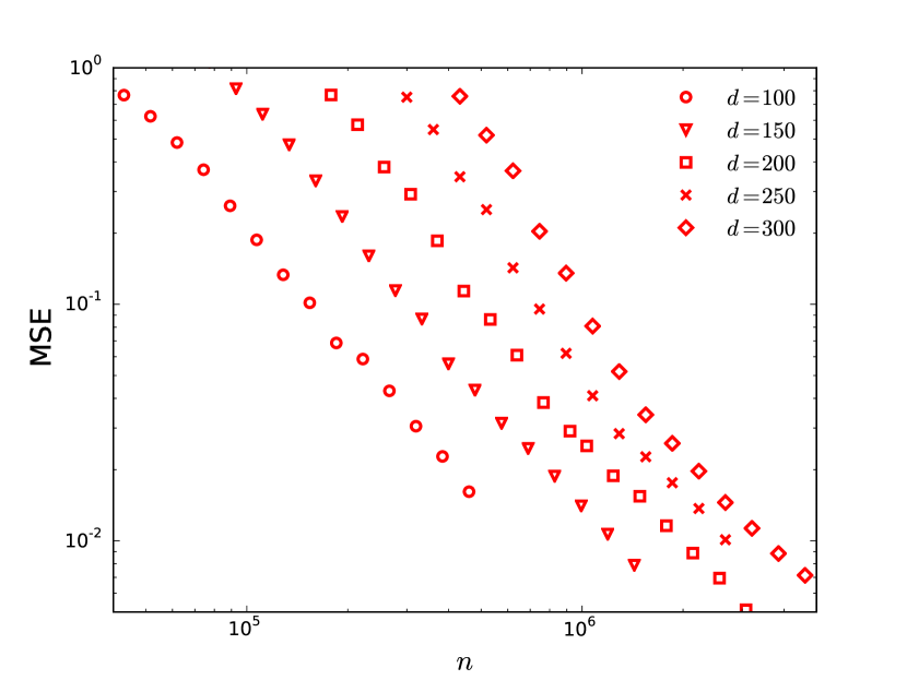
(a) Estimated MSE vs. sample size n.

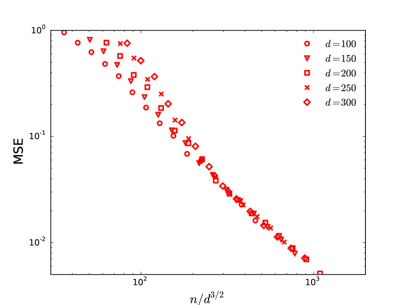
(b) Estimated MSE vs. rescaled sample size $\textsf{n}/d^{3/2}$.

Figure 1. Numerical illustration of Algorithm 1 for completing random tensors (18) of order $k=3$ and rank $r=4$. Performance is measured in terms of normalized mean squared error MSE (see (19)), estimated by averaging over $100$ realizations.

5.2. Performance of spectral algorithm for overcomplete tensors

Figure 2 reports the performance of our spectral method for the overcomplete regime (Algorithm 2), taking $r/d=1.2$. We set $\lambda_{\star}$ according to the prescription (16) of Theorem 2. For each value of $d$, the MSE appears to decrease rapidly with n. The plots (for various values of $d$) of the MSE versus the rescaled sample size $\textsf{n}/(rd^{3/2})$ appears to approach a limiting curve. This suggests that the threshold for our method to succeed in reconstruction occurs around $\textsf{n}=rd^{3/2}$, which is consistent with the bound of our Theorem 2.

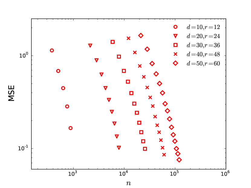
(a) Estimated MSE vs. sample size n.

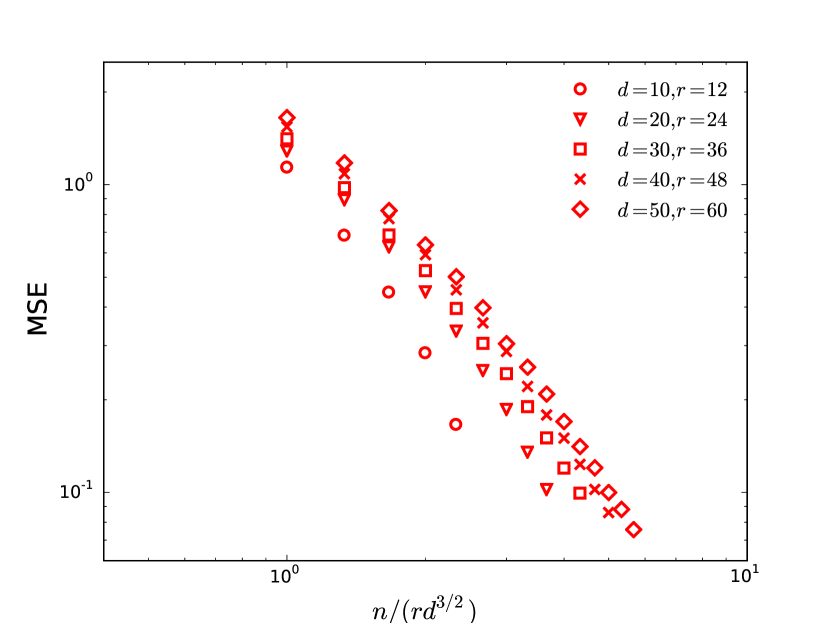
(b) Estimated MSE vs. rescaled sample size $\textsf{n}/d^{3/2}$.

Figure 2. Performance of Algorithm 2 in completing overcomplete random tensors of rank $4$, and order $k=3$. Left frame: mean square error of reconstruction, estimated by averaging over $100$ realizations, plotted against the number of revealed entries. Right frame: same data plotted against the rescaled number of revealed entries $\textsf{n}/(rd^{3/2})$.

6. Column spaces of partially revealed wide matrices

In this section we present our results on the column spaces of partially revealed $d_{1}\times d_{2}$ matrices. As mentioned above, these results are the main input to the proof of Theorem 1. The conclusions obtained in this section are most interesting for the regime $d_{1}\ll d_{2}$.

6.1. Incoherence condition

Assumption 3.

We say that a matrix $X\in\mathbb{R}^{d_{1}\times d_{2}}$ is $(\lambda,\gamma,\rho)$-incoherent if

1. $d_{1}\cdot\max_{i}\|X^{\sf t}e_{i}\|^{2}\leq\lambda\|X\|_{\textup{op}}^{2}$;

2. $d_{2}\cdot\max_{j}\|Xe_{j}\|^{2}\leq\rho\|X\|_{\textup{op}}^{2}$; and

3. $d_{1}d_{2}\cdot\max_{i,j}|X_{i,j}|^{2}\leq\lambda\gamma\rho\|X\|_{\textup{op}}^{2}$,

where $1\leq i\leq d_{1}$ and $1\leq j\leq d_{2}$.

It is easily seen (cf. Lemma 10) that one can assume without loss of generality $1/d_{1}\leq\lambda\leq d_{1}$, $1/d_{2}\leq\rho\leq d_{2}$, $1\leq\lambda\gamma\rho\leq d_{1}d_{2}$. To motivate the above condition, we observe that it can be deduced as a consequence of a standard incoherence assumption, that we recall below.

Definition 2 ([CR09]).

Let $W$ be an $r$-dimensional subspace of $\mathbb{R}^{d}$, and let $P_{W}$ be the orthogonal projection onto $W$. The coherence of $W$ (with respect to the standard basis $(e_{i})_{i\leq d}$ of $\mathbb{R}^{d}$) is

$$\textup{{coher}}_{W}=\frac{d}{r}\max_{1\leq i\leq d}\|P_{W}e_{i}\|^{2}\,.$$

Note the trivial bounds

$$\frac{d}{r}\geq\textup{{coher}}_{W}\geq\frac{1}{r}\sum_{i=1}^{d}\|P_{W}e_{i}\|^{2}=1\,.$$

If $M$ is a $d\times r$ matrix whose columns form an orthonormal basis of $W$, then we can express $P_{W}=MM^{\sf t}$, so that

$$\textup{{coher}}_{W}=\frac{d}{r}\max_{1\leq i\leq d}\|MM^{\sf t}e_{i}\|^{2}=\frac{d}{r}\max_{1\leq i\leq d}\sum_{s=1}^{r}(M_{is})^{2}\,.$$

We denote $\textup{{coher}}_{M}\equiv\textup{{coher}}_{W}$.

We refer to [CR09] for further discussion of this coherence condition, which has become fairly standard in the literature. We now give two illustrations for Assumption 3:

1. Derivation of Assumption 3 from Definition 2.
   Suppose $X$ is $d_{2}\times d_{2}$ with singular value decomposition $UDV^{\sf t}$, where $U^{\sf t}U=I_{\textup{{r}}}=V^{\sf t}V$ and $D$ is diagonal. One can then easily verify that $X$ is $(\lambda,\gamma,\rho)$-incoherent with

   $$\lambda=(\textup{{coher}}_{U})\textup{{r}},\quad\rho=(\textup{{coher}}_{V})\textup{{r}},\quad\gamma=1\,.$$ (21)

   (see Lemma 9 for the proof). That is to say, imposing Assumption 3 with $\lambda=\rho=c\textup{{r}}$ and $\gamma=1$ is less restrictive than imposing that $X$ is of rank r with $c$-incoherent singular vectors.

2. Derivation of Assumption 3 from Assumption 1.
   Alternatively, suppose $X$ satisfies an entrywise bound $d_{1}d_{2}\|X\|_{\infty}^{2}\leq\bar{\varpi}\|X\|_{\textup{op}}^{2}$. It is then trivial to verify that $X$ is $(\lambda,\gamma,\rho)$-incoherent with

   $$\lambda=\rho=1/\gamma=\bar{\varpi}.$$ (22)

   In Assumption 1, conditions T2 and T3 together imply (with $d_{1}=d^{a}$ and $d_{2}=d^{b}$)

   $$d_{1}d_{2}\|X\|_{\infty}^{2}\leq\alpha\|X\|_{\textup{F}}^{2}\leq(\alpha\textup{{r}}/\mu)\|X\|_{\textup{op}}^{2}\,,$$

   so we have (22) with $\bar{\varpi}=\alpha\textup{{r}}/\mu$. That is to say, imposing Assumption 3 with $\lambda=\rho=1/\gamma=\alpha\textup{{r}}/\mu$ is less restrictive than imposing Assumption 1 with parameters $(\textup{{r}},\alpha,\mu)$.

In the tensor completion problem we work with the second scenario (22).

6.2. Estimation error

We now state our main result on column space estimation for partially revealed matrices.

Theorem 3.

Suppose that $X\in\mathbb{R}^{d_{1}\times d_{2}}$ is $(\lambda,\gamma,\rho)$-incoherent. Let $\textup{{E}}\subseteq[d_{1}]\times[d_{2}]$ be the random set of observed entries, where each $(i,j)\in[d_{1}]\times[d_{2}]$ is included in E independently with probability $\delta=\textsf{n}/(d_{1}d_{2})$. Given the observed matrix $Y\equiv\Pi_{\textup{{E}}}X$, let

$$\widehat{B}\equiv\frac{1}{\delta}\Pi(YY^{\sf t})+\frac{1}{\delta^{2}}\Pi_{\perp}(YY^{\sf t})\,.$$ (23)

Then, for $d_{1}d_{2}\geq 3000$, we have

$$\frac{\|\widehat{B}-XX^{\sf t}\|_{\textup{op}}}{2(\log(d_{1}d_{2}))^{4}}\leq\frac{(\lambda\rho d_{1}d_{2})^{1/2}\|X\|_{\textup{op}}^{2}}{\textsf{n}}\max\bigg{\{}1\,,\bigg{(}\frac{\textsf{n}}{d_{2}\lambda}\bigg{)}^{1/2}\,,\frac{(\lambda\gamma^{2}\rho d_{1}d_{2})^{1/2}}{\textsf{n}}\,,\bigg{(}\frac{\lambda\rho}{d_{2}}\bigg{)}^{1/2}\bigg{\}}$$ (24)

with probability at least $1-4d_{1}\exp\{-\tfrac{1}{8}\log(d_{1}d_{2})^{2}\}$.

Corollary 3.

In the setting of Theorem 3, assume additionally that $(\lambda\gamma^{2}\rho d_{1}d_{2}/t)^{1/2}\leq\textsf{n}\leq t\lambda d_{2}$ and $\gamma\rho\leq td_{2}$. Then the error bound (24) simplifies to

$$\frac{\|\widehat{B}-XX^{\sf t}\|_{\textup{op}}}{2(\log(d_{1}d_{2}))^{4}}\leq\frac{(t\lambda\rho d_{1}d_{2})^{1/2}}{\textsf{n}}\|X\|_{\textup{op}}^{2}\,.$$

Proof.

Immediate consequence of Theorem 3. ∎

From our perspective, the most interesting application of the above is as follows. Recalling (21), suppose the $d_{1}\times d_{2}$ matrix $X$ is $(\lambda,\gamma,\rho)$-incoherent with $\lambda=\rho=cr$ and $\gamma=1$. Consider Corollary 3 with $t=1$: then the conditions reduce to $cr\leq(d_{2})^{1/2}$ and $cr(d_{1}d_{2})^{1/2}\leq\textsf{n}\leq crd_{2}$, where the latter can only be satisfied if $d_{1}\leq d_{2}$. With these conditions, Corollary 3 says that the column space of $X$ can be well approximated by the top eigenvectors of the matrix $\widehat{B}$, provided we saw (roughly) $\textsf{n}\gg r(d_{1}d_{2})^{1/2}$ entries. We emphasize that this result implies, for $d_{1}\ll d_{2}$, a wide regime of sample sizes

$$r(d_{1}d_{2})^{1/2}\ll\textsf{n}\ll rd_{2}$$

from which we can obtain a good estimate of the sample space, even though it is impossible to complete the matrix (in the sense of Frobenius norm approximation). In this regime, the column space estimate can be useful for (partial) matrix completion: if $Q$ approximates projection onto the left column space of $X$, and $y$ is a column of $\Pi_{\textup{{E}}}X$ containing $d\delta^{\prime}\gg r$ observed entries, then $Qy/\delta^{\prime}$ is a good estimate of the corresponding column of $X$.

Acknowledgements

This research was partially supported by NSF grant CCF-1319979 (A.M.) and NSF MSPRF grant DMS-1401123 (N.S.).

Appendix A Standard matrix inequalities

In this appendix we collect a few standard tools that will be used several times in our proofs. For any real-valued random variable $X$, the essential supremum $\operatorname{ess\,sup}X$ is the minimal value $R$ such that $\mathbb{P}(X\leq R)=1$. Recall the following form of the Chernoff bound: if $X$ is a binomial random variable with mean $\bar{\mu}$, then for all $t\geq 1$ we have

$$\mathbb{P}(X\geq t\bar{\mu})\leq\exp\{-t\bar{\mu}\log(t/e)\}\,.$$ (25)

Proposition 4 (matrix Bernstein, rectangular [Tro12, Theorem 1.6]).

Let $(Z_{\ell})$ be a finite sequence of independent random $d_{1}\times d_{2}$ matrices. Assume $\mathbb{E}Z_{\ell}=0$ for all $\ell$, and let

$$R=\max_{\ell}\bigg{\{}\operatorname{ess\,sup}\|Z_{\ell}\|_{\textup{op}}\bigg{\}}\,,\quad\sigma^{2}=\max\bigg{\{}\bigg{\|}\sum_{\ell}\mathbb{E}[Z_{\ell}(Z_{\ell})^{{\sf t}}]\bigg{\|}_{\textup{op}},\bigg{\|}\sum_{\ell}\mathbb{E}[(Z_{\ell})^{{\sf t}}Z_{\ell}]\bigg{\|}_{\textup{op}}\bigg{\}}\,.$$ (26)

Then, for all $t\geq 0$,

$$\mathbb{P}\bigg{(}\bigg{\|}\sum_{\ell}Z_{\ell}\bigg{\|}_{\textup{op}}\geq t\bigg{)}\leq(d_{1}+d_{2})\exp\bigg{\{}-\frac{3}{8}\min\bigg{\{}\frac{t^{2}}{\sigma^{2}},\frac{t}{R}\bigg{\}}\bigg{\}}\,.$$

Proposition 5 ([Wed72]).

Suppose that $\mathcal{A}$ and $\mathcal{B}$ are positive semidefinite matrices, with singular value decompositions

$$\begin{array}[]{rll}\mathcal{A}=A+A_{\circ}&=U\Sigma U^{\sf t}+U_{\circ}\Sigma_{\circ}(U_{\circ})^{\sf t},&\begin{pmatrix}U&U_{\circ}\end{pmatrix}^{\sf t}\begin{pmatrix}U&U_{\circ}\end{pmatrix}=I_{r},\\ \mathcal{B}=B+B_{\circ}&=O\Lambda O^{\sf t}+O_{\circ}\Lambda_{\circ}(O_{\circ})^{\sf t},&\begin{pmatrix}O&O_{\circ}\end{pmatrix}^{\sf t}\begin{pmatrix}O&O_{\circ}\end{pmatrix}=I_{s}.\end{array}$$

Suppose $\|\mathcal{A}-\mathcal{B}\|_{\textup{op}}\leq\epsilon$, and that the maximum diagonal entry of $\Sigma_{\circ}$ is at most $\sigma$ while the minimum diagonal entry of $\Lambda$ is at least $\sigma+\delta>0$. Then

$$|\sin\theta(O,U)|\equiv\|(I-UU^{\sf t})OO^{\sf t}\|_{\textup{op}}\leq\epsilon/\delta\,.$$

Proposition 6 ([HSSS15, Propn. A.7]).

Let $(Z_{\ell})_{\ell\leq L}$ be a sequence of independent random $d_{1}\times d_{2}$ matrices. Assume $\mathbb{E}Z_{\ell}=0$ for all $\ell$, and furthermore that

$$\mathbb{P}(\|Z_{\ell}\|_{\textup{op}}\geq\beta)\leq p\quad\text{and}\quad\|\mathbb{E}[Z_{\ell}\mathbf{1}\{\|Z_{\ell}\|_{\textup{op}}\geq\beta\}]\|_{\textup{op}}\leq q\,.$$ (27)

Denote $\sigma^{2}$ as in (26). Then, for all $t\geq 0$,

$$\mathbb{P}\bigg{(}\bigg{\|}\sum_{\ell\leq L}Z_{\ell}\bigg{\|}_{\textup{op}}\geq t+Lq\bigg{)}\leq Lp+(d_{1}+d_{2})\exp\bigg{\{}-\frac{3}{8}\min\bigg{\{}\frac{t^{2}}{\sigma^{2}},\frac{t}{\beta}\bigg{\}}\bigg{\}}\,.$$

Proposition 7 (matrix Rademacher, symmetric [Tro12, Thm. 1.2]).

Let $(Z_{\ell})$ be a finite sequence of $d\times d$ symmetric matrices. Let $(\mathfrak{s}_{\ell})$ be a sequence of independent symmetric random signs. Then

$$\mathbb{P}\bigg{(}\bigg{\|}\sum_{\ell}\mathfrak{s}_{\ell}Z_{\ell}\bigg{\|}_{\textup{op}}\geq t\bigg{)}\leq 2d\exp\{-t^{2}/(2\sigma^{2})\},\quad\sigma^{2}=\bigg{\|}\sum_{\ell}(Z_{\ell})^{2}\bigg{\|}_{\textup{op}}\,.$$

Proposition 8 (matrix decoupling [dlPMS95, Thm. 1] (see also [HSSS15, Thm. 5.13])).

Let $(Z_{ij})$ be a family of matrices, and let $(\mathfrak{s}_{i})$ and $(\mathfrak{t}_{i})$ be sequences of independent symmetric random signs. There is an absolute constant $C$ such that for all $t\geq 0$,

$$\mathbb{P}\bigg{(}\bigg{\|}\sum_{i\neq j}\mathfrak{s}_{i}\mathfrak{s}_{j}Z_{ij}\bigg{\|}_{\textup{op}}\geq t\bigg{)}\leq C\mathbb{P}\bigg{(}\bigg{\|}\sum_{i\neq j}\mathfrak{s}_{i}\mathfrak{t}_{j}Z_{ij}\bigg{\|}_{\textup{op}}\geq t\bigg{)}\,.$$

Appendix B Column space estimation with large aspect ratios

In this appendix, we prove our matrix completion result, Theorem 3. Before passing to the actual proof, we will establish some properties of the incoherence condition, Assumption 3.

B.1. Matrix incoherence conditions

We begin by proving some easy observations regarding our matrix incoherence conditions (Assumption 3).

Lemma 9.

Suppose $X\in\mathbb{R}^{d_{1}\times d_{2}}$ has singular value decomposition $UDV^{\sf t}$, with $U^{\sf t}U=I_{r}=V^{\sf t}V$. Then $X$ is $(\lambda,\gamma,\rho)$-incoherent with parameters $\lambda=r\cdot\textup{{coher}}_{U}$, $\rho=r\cdot\textup{{coher}}_{V}$, and $\gamma=1$.

Proof.

For indices $1\leq i\leq d_{1}$ and $1\leq\ell\leq d_{2}$ we have

$$|X_{i\ell}| =|\langle UU^{\sf t}e_{i},XVV^{\sf t}e_{\ell}\rangle|\leq\|X\|_{\textup{op}}\Big{(}\frac{r^{2}\cdot\textup{{coher}}_{U}\cdot\textup{{coher}}_{V}}{d_{1}d_{2}}\Big{)}^{1/2}\,,$$

$$\|X^{\sf t}e_{i}\|_{2} =\|X^{\sf t}UU^{\sf t}e_{i}\|_{2}\leq\|X\|_{\textup{op}}\|UU^{\sf t}e_{i}\|_{2}\leq\|X\|_{\textup{op}}\Big{(}\frac{r\cdot\textup{{coher}}_{U}}{d_{1}}\Big{)}^{1/2}\,,$$

$$\|Xe_{\ell}\|_{2} =\|XVV^{\sf t}e_{\ell}\|_{2}\leq\|X\|_{\textup{op}}\|VV^{\sf t}e_{\ell}\|_{2}\leq\|X\|_{\textup{op}}\Big{(}\frac{r\cdot\textup{{coher}}_{V}}{d_{2}}\Big{)}^{1/2}\,,$$

which proves the claim. ∎

Lemma 10.

For any $X\in\mathbb{R}^{d_{1}\times d_{2}}$, the parameters $\lambda,\gamma,\rho$ of Assumption 3 can be chosen so that

$$1/d_{1}\leq\lambda\leq d_{1},\ 1/d_{2}\leq\rho\leq d_{2},\ 1\leq\lambda\gamma\rho\leq d_{1}d_{2}\,.$$ (28)

Proof.

The quantities $\|X^{\sf t}e_{i}\|$, $\|Xe_{\ell}\|$, $|X_{i\ell}|$ are all trivially upper bounded by $\|X\|_{\textup{op}}$, so we can always satisfy M1, M2, M3 with $\lambda\leq d_{1}$, $\rho\leq d_{2}$, and $\lambda\gamma\rho\leq d_{1}d_{2}$. On the other hand

$$\|X\|_{\textup{op}}=\bigg{\|}\sum_{\ell\leq d_{2}}Xe_{\ell}(e_{\ell})^{\sf t}\bigg{\|}_{\textup{op}}\leq\sum_{\ell\leq d_{2}}\|Xe_{\ell}\|_{2}\leq\|X\|_{\textup{op}}(d_{2}\rho)^{1/2}\,,$$

which implies that M2 can only be satisfied with $d_{2}\rho\geq 1$, and likewise M1 can only be satisfied with $d_{1}\lambda\geq 1$. Lastly, we have

$$\|X\|_{\textup{op}}\leq\|X\|_{\textup{F}}\leq(d_{1}d_{2})^{1/2}\max_{i,\ell}|X_{i,\ell}|\leq\|X\|_{\textup{op}}(\lambda\gamma\rho)^{1/2}\,,$$

so M3 can only be satisfied with $\lambda\gamma\rho\geq 1$. This concludes the justification of (28). ∎

B.2. Proof of matrix estimation results

We now prove Theorem 3. Recall that we assume a (deterministic) matrix $X\in\mathbb{R}^{d_{1}\times d_{2}}$, each entry of which is observed independently with chance $\delta\equiv\textsf{n}/(d_{1}d_{2})$. Let $\textup{{E}}\subseteq[d_{1}]\times[d_{2}]$ denote the subset of observed entries, and $Y=\Pi_{\textup{{E}}}X$ the partially observed matrix. Let $I_{i\ell}$ be the indicator that $(i,\ell)$ belongs to the (random) set E; thus the $I_{i\ell}$ are i.i.d. $\mathrm{Ber}(\delta)$ random variables and $Y_{i\ell}=X_{i\ell}I_{i\ell}$. As in (23), let

$$\widehat{B}=\frac{1}{\delta}\Pi(YY^{\sf t})+\frac{1}{\delta^{2}}\Pi_{\perp}(YY^{\sf t})\,.$$

Proof of Theorem 3.

We first make a preliminary remark that

$$1\leq\frac{1}{\delta^{2}}\leq\frac{(d_{1}\lambda)(d_{2}\rho)}{(\lambda\gamma\rho)^{2}}\leq(d_{1}d_{2})^{2}\,.$$ (29)

(The second inequality follows from the assumptions, while the third follows from Lemma 10.) We shall apply Proposition 6 to bound the spectral norm of

$$\widehat{B}-XX^{\sf t}=\widehat{B}-\mathbb{E}\widehat{B}=\sum_{\ell\leq d_{2}}(B_{\ell}-\mathbb{E}B_{\ell})=\sum_{\ell\leq d_{2}}Z_{\ell}\,,$$ (30)

where $B_{\ell}$ is $d_{1}\times d_{1}$ with entries

$$(B_{\ell})_{ij}=\left\{\begin{array}[]{ll}\delta^{-1}(X_{i\ell})^{2}I_{i\ell}&\textup{for }i=j\,,\\ \delta^{-2}X_{i\ell}X_{j\ell}I_{i\ell}I_{j\ell},&\textup{for }i\neq j\,.\\ \end{array}\right.$$

Lemmas 11 and 12 (below) show that the matrices $Z_{\ell}$ satisfy the hypotheses of Proposition 6 with $\sigma^{2}$ as in (31) and $\beta,p,q$ as in (32), for $d_{1}d_{2}$ sufficiently large. We then have

$$3\min\bigg{\{}\frac{t^{2}}{\sigma^{2}},\frac{t}{\beta}\bigg{\}}\geq\log(d_{1}d_{2})^{2}$$

provided $t\geq t_{\max}\equiv(\log(d_{1}d_{2}))^{4}\max\{t_{1},t_{2},t_{3},t_{4}\}\|X\|_{\textup{op}}^{2}$ for

$$t_{1} =\bigg{(}\frac{\lambda\rho}{d_{1}d_{2}\delta^{2}}\bigg{)}^{1/2}=\bigg{(}\frac{\lambda}{d_{1}\delta}\bigg{)}^{1/2}\bigg{(}\frac{\rho}{d_{2}\delta}\bigg{)}^{1/2}\,,$$

$$t_{2} =\bigg{(}\frac{\rho}{d_{2}\delta}\bigg{)}^{1/2}=t_{1}\bigg{(}\frac{d_{1}\delta}{\lambda}\bigg{)}^{1/2}\,,$$

$$t_{3} =\frac{\lambda\gamma\rho}{d_{1}d_{2}\delta^{2}}=\bigg{(}\frac{\lambda\rho}{d_{1}d_{2}\delta^{2}}\bigg{)}^{1/2}\bigg{(}\frac{\lambda\gamma^{2}\rho}{d_{1}d_{2}\delta^{2}}\bigg{)}^{1/2}=t_{1}\bigg{(}\frac{\lambda\gamma^{2}\rho}{d_{1}d_{2}\delta^{2}}\bigg{)}^{1/2}\,,$$

$$t_{4} =\frac{(\lambda\gamma)^{1/2}\rho}{(d_{1})^{1/2}d_{2}\delta}=\bigg{(}\frac{\lambda\rho}{d_{1}d_{2}\delta^{2}}\bigg{)}^{1/2}\bigg{(}\frac{\gamma\rho}{d_{2}}\bigg{)}^{1/2}=t_{1}\bigg{(}\frac{\gamma\rho}{d_{2}}\bigg{)}^{1/2}\,.$$

From (32) we have $t_{\max}\geq\beta_{\star}\geq d_{2}q$. It follows from Proposition 6 that

$$\mathbb{P}(\|\widehat{B}-\mathbb{E}\widehat{B}\|_{\textup{op}}\geq 2t_{\max})\leq\frac{2d_{1}d_{2}}{\exp\{\tfrac{3}{8}\log(d_{1}d_{2})^{2}\}}+\frac{2d_{1}}{\exp\{\tfrac{1}{8}\log(d_{1}d_{2})^{2}\}}\leq\frac{4d_{1}}{\exp\{\tfrac{1}{8}\log(d_{1}d_{2})^{2}\}}\,,$$

which concludes the proof. ∎

Lemma 11.

Assume the setting and notation of Theorem 3, and let $Z_{\ell}$ be as defined by (30). For $\sigma^{2}$ as defined by (26), we have

$$\sigma^{2}\leq 2\max\bigg{\{}\frac{\lambda\rho}{d_{1}d_{2}\delta^{2}},\frac{\rho}{d_{2}\delta}\bigg{\}}\|X\|_{\textup{op}}^{4}\,.$$ (31)

Proof.

From the definitions, we have

$$(Z_{\ell})_{ij}=\left\{\begin{array}[]{ll}\delta^{-1}(X_{i\ell})^{2}(I_{i\ell}-\delta)&\textup{for }i=j\\ \delta^{-2}X_{i\ell}X_{j\ell}(I_{i\ell}I_{j\ell}-\delta^{2})&\textup{for }i\neq j\,.\end{array}\right.$$

Recalling (26), let $\Sigma$ denote the sum of the matrices $\mathbb{E}[(Z_{\ell})^{2}]$ over $\ell\leq d_{2}$. Let $W$ denote the $d_{2}\times d_{2}$ diagonal matrix with entries $W_{\ell\ell}=\|Xe_{\ell}\|^{2}$. It is straightforward to compute that

$$\Sigma=\frac{1-\delta}{\delta^{2}}D+\frac{1-\delta}{\delta}XWX^{\sf t}$$

where $D$ is the $d_{1}\times d_{1}$ diagonal matrix with entries

$$D_{ii}=\sum_{\ell\leq d_{2}}(X_{i\ell})^{2}\Big{(}\|Xe_{\ell}\|^{2}-(X_{i\ell})^{2}\Big{)}\,.$$

We then note $\|XWX^{\sf t}\|_{\textup{op}}\leq\|X\|_{\textup{op}}^{2}\|W\|_{\textup{op}}\leq\rho\|X\|_{\textup{op}}^{4}/d_{2}$, while

$$0\leq D_{ii}\leq\frac{\rho\|X\|_{\textup{op}}^{2}\|X^{\sf t}e_{i}\|^{2}}{d_{2}}\leq\frac{\lambda\rho\|X\|_{\textup{op}}^{4}}{d_{1}d_{2}}\,.$$

Combining the above estimates, we find

$$\|\Sigma\|_{\textup{op}}\leq\frac{\|D\|_{\textup{op}}}{\delta^{2}}+\frac{\|XWX^{\sf t}\|_{\textup{op}}}{\delta}\leq\frac{\lambda\rho\|X\|_{\textup{op}}^{4}}{d_{1}d_{2}\delta^{2}}+\frac{\rho\|X\|_{\textup{op}}^{4}}{d_{2}\delta}\,,$$

yielding the claimed bound. ∎

Lemma 12.

Assume the setting and notation of Theorem 3, and let $Z_{\ell}$ be as defined by (30). Let

$$\beta_{\star}\equiv\max\bigg{\{}\frac{\lambda\gamma\rho}{d_{1}d_{2}\delta^{2}}\,,\frac{(\lambda\gamma)^{1/2}\rho}{(d_{1})^{1/2}d_{2}\delta}\bigg{\}}\|X\|_{\textup{op}}^{2}\,.$$

For $d_{1}d_{2}\geq 3000$, the matrices $Z_{\ell}$ satisfy (27) with

$$\begin{array}[]{rl}\beta&=(\log(d_{1}d_{2}))^{2}\beta_{\star}\,,\\ p&=\exp\{-(3/8)(\log(d_{1}d_{2}))^{2}\}\cdot 2d_{1}\,,\\ q&=\exp\{-(1/8)(\log(d_{1}d_{2}))^{2}\}\cdot\beta_{\star}\,.\end{array}$$ (32)

Proof.

Write $e_{i}$ for the $i$-th standard basis vector in $\mathbb{R}^{d_{1}}$, and let $E_{ij}\equiv e_{i}(e_{j})^{\sf t}$. Then $Z_{\ell}$ is the sum of independent zero-mean matrices $M_{ij}=E_{ii}(Z_{\ell})_{ii}$. It is straightforward to calculate that It follows from the matrix Bernstein inequality (Proposition 4) that

$$\mathbb{P}(\|Z_{\ell}\|_{\textup{op}}\geq t)\leq 2d_{1}\exp\bigg{\{}-\frac{3}{8}\min\bigg{\{}\frac{t^{2}}{\sigma^{2}},\frac{t}{R}\bigg{\}}\bigg{\}}$$

where (cf. (26)) $R,\sigma$ are given by

$$\sigma =\frac{\|X\|_{\infty}\|Xe_{\ell}\|}{\delta}\leq\frac{(\lambda\gamma)^{1/2}\rho}{(d_{1})^{1/2}d_{2}}\frac{\|X\|_{\textup{op}}^{2}}{\delta}\leq d_{1}d_{2}\|X\|_{\textup{op}}^{2}\,,$$

$$R =\frac{\|X\|_{\infty}^{2}}{\delta^{2}}\leq\frac{\lambda\gamma\rho}{d_{1}d_{2}}\frac{\|X\|_{\textup{op}}^{2}}{\delta^{2}}\leq(d_{1}d_{2})^{2}\|X\|_{\textup{op}}^{2}\,,$$

having made use of Lemma 10 and (29). If we set $\beta_{\star}=\max\{\sigma,R\}$ and $\beta=(\log(d_{1}d_{1}))^{2}\beta_{\star}$, then

$$\mathbb{P}(\|Z_{\ell}\|_{\textup{op}}\geq\beta)\leq 2d_{1}\exp\{-\tfrac{3}{8}(\log(d_{1}d_{1}))^{2}\}=p\,.$$

Next note that for $t\geq\max\{\sigma,R\}$ we have $\min\{t^{2}/\sigma^{2},t/R\}\geq t/\max\{\sigma,R\}$, so

$$\mathbb{E}[\|Z_{\ell}\|_{\textup{op}};\|Z_{\ell}\|_{\textup{op}}\geq\beta]\leq\beta p+\int_{\beta}^{\infty}\mathbb{P}(\|Z_{\ell}\|_{\textup{op}}\geq t)\,dt\leq\beta p+2d_{1}\int_{\beta}^{\infty}\exp\bigg{\{}-\frac{(3/8)t}{\max\{\sigma,R\}}\bigg{\}}\,dt$$

$$\qquad=\frac{[(\log(d_{1}d_{2}))^{2}+\tfrac{8}{3}]2d_{1}\max\{R,\sigma\}}{\exp\{\tfrac{3}{8}(\log(d_{1}d_{2}))^{2}\}}\leq\frac{(d_{1}d_{2})^{2}\max\{R,\sigma\}}{\exp\{\tfrac{3}{8}(\log(d_{1}d_{2}))^{2}\}}\leq\frac{\max\{R,\sigma\}}{\exp\{\tfrac{1}{8}(\log(d_{1}d_{2}))^{2}\}}=q\,.$$

This concludes the proof. ∎

Appendix C Tensor completion via unfolding

In this section we prove Theorem 1. In the original model, we observe exactly $\delta=|\textup{{E}}|/d^{k}$ fraction of the entries, uniformly at random. For convenience we now introduce the Bernoulli model where each entry is observed independently with chance $\delta$. Our results for the Bernoulli model transfer to the original model by a standard argument, which we provide below.

As in Theorem 1, suppose $\bm{T}\in(\mathbb{R}^{d})^{\otimes k}$ is a deterministic symmetric tensor satisfying Assumption 1 with unfolding parameters $(\textup{{r}},\alpha,\mu)$. Fixing $\delta\in(0,1)$, let $\delta_{1}\equiv\delta/2$ and $\delta_{2}\equiv\delta_{1}/(1-\delta_{1})$. Let $\{I_{\underline{\smash{u}}},J_{\underline{\smash{u}}}\}$ be a collection of independent random variables (indexed by ${\underline{\smash{u}}}\in[d]^{k}$) with $I_{\underline{\smash{u}}}\sim{\rm Ber}(\delta_{1})$ and $J_{\underline{\smash{u}}}\sim{\rm Ber}(\delta_{2})$. Let $\textup{{E}}_{1}$ be the set of ${\underline{\smash{u}}}\in[d]^{k}$ with $I_{\underline{\smash{u}}}=1$; and let $\textup{{E}}_{2}$ be the set of ${\underline{\smash{u}}}\in[d]^{k}$ with $(1-I_{\underline{\smash{u}}})J_{\underline{\smash{u}}}=1$. Define the corresponding partially observed tensors $\bm{Y}_{i}=\Pi_{\textup{{E}}_{i}}(\bm{T})$. Fixing integers $1\leq a\leq b=k-a$, let $X=\textup{{unfold}}^{a\times b}(\bm{T})$, $Z=\textup{{unfold}}^{a\times b}(\bm{Y}_{1})$, and (cf. (9))

$$B=\frac{1}{\delta_{1}}\Pi(ZZ^{\sf t})+\frac{1}{(\delta_{1})^{2}}\Pi_{\perp}(ZZ^{\sf t}).$$ (33)

Let $Q$ be the orthogonal projection onto the span of onto the eigenspace of $B$ for eigenvalues $\geq\lambda_{\star}$. If $a=\lfloor k/2\rfloor$, then we can use $Q$ to define ${\mathcal{Q}}$ as in (10). Then let

$${\widehat{\bm{T}}}\equiv\bm{Y}_{1}+\frac{1}{\delta_{2}}\bm{Y}_{2},\quad\bm{T}^{\star}={\mathcal{Q}}(\widehat{T}),\quad\widehat{\bm{T}}^{\star}={\mathcal{Q}}({\widehat{\bm{T}}})\,;$$ (34)

and note that $\mathbb{E}[{\widehat{\bm{T}}}\,|\,\textup{{E}}_{1}]=\bm{T}$. Define

$$\varpi\equiv\frac{\alpha\textup{{r}}}{\mu}\,,\quad\vartheta\equiv\frac{\alpha\textup{{r}}}{\delta d^{k/2}}\,,\quad\eta(t)\equiv\frac{8(k\log d)^{4}t^{1/2}\varpi}{d^{k/2}\delta}\,,\quad\lambda_{\star}(t)\equiv\eta^{2/3}\|B\|_{\textup{op}}\,.$$ (35)

We will consider $\widehat{\bm{T}}^{\star}$ with threshold $\lambda_{\star}=\lambda_{\star}(t)$ as given by (35).

Theorem 4.

Suppose $\bm{T}\in(\mathbb{R}^{d})^{\otimes k}$ is a deterministic symmetric tensor satisfying Assumption 1 with unfolding parameters $(\textup{{r}},\alpha,\mu)$, such that $\textup{{r}}\leq r_{\max}$ as defined by (11). Fix $t\geq 1$ and suppose

$$\frac{32(k\log d)^{4}t^{1/2}\varpi}{d^{k/2}}\leq\delta\leq\frac{t\varpi}{d^{a}}$$ (36)

Then, with $\smash{\widehat{\bm{T}}^{\star}}$ as above, we have

$$\|\bm{T}-\widehat{\bm{T}}^{\star}\|_{\textup{F}}\leq 20(k\log d)^{4/3}(t\mu)^{1/6}\vartheta^{1/3}\|\bm{T}\|_{\textup{F}}$$

with probability at least $1-3d^{k}\exp\{-\tfrac{1}{8}(k\log d)^{2}\}$.

Let us discuss the choice of $t$ in Theorem 4. We wish to have a small error $\|\bm{T}-\widehat{\bm{T}}^{\star}\|_{\textup{F}}$, while ensuring that condition (36) is satisfied. First note that (36) cannot be satisifed at all unless we have $t^{1/2}\geq 32(k\log d)^{4}/d^{k/2-a}$. If we take $\epsilon\leq 1$ and set

$$\delta=\frac{20^{3}(k\log d)^{4}t^{1/2}\mu^{3/2}\varpi}{\epsilon^{3}d^{k/2}}\,,$$

then Theorem 4 gives $\|\bm{T}-\widehat{\bm{T}}^{\star}\|_{\textup{F}}\leq\epsilon\|\bm{T}\|_{\textup{F}}$. This choice of $\delta$ automatically satisfies the lower bound of (36). To satisfy the upper bound we require

$$t^{1/2}\geq\frac{20^{3}(k\log d)^{4}\mu^{3/2}}{\epsilon^{3}d^{k/2-a}}\,.$$

Since $a\leq k/2$ and we aim for $\epsilon\leq 1/(k\log d)$ in the worse case, we shall set $t^{1/2}=(k\log d)^{8}\mu^{3/2}$. With this choice, (36) simplifies to

$$\frac{32(k\log d)^{12}\alpha\textup{{r}}\mu^{1/2}}{d^{k/2}}\leq\delta\leq\frac{(k\log d)^{16}\alpha\textup{{r}}\mu^{2}}{d^{a}}\,,$$

and we obtain $\|\bm{T}-\widehat{\bm{T}}^{\star}\|_{\textup{F}}\leq\epsilon\|\bm{T}\|_{\textup{F}}$ with

$$\lambda_{\star}=4(k\log d)^{8}\bigg{(}\frac{\alpha\textup{{r}}\mu^{1/2}}{d^{k/2}\delta}\bigg{)}^{2/3}\|B\|_{\textup{op}}\,,\quad\epsilon=20(k\log d)^{3}\bigg{(}\frac{\alpha\textup{{r}}\mu^{2}}{d^{k/2}\delta}\bigg{)}^{1/3}\,.$$

Then, as noted previously, the result of Theorem 4 (for the Bernoulli model) implies the result of Theorem 1 (for the original model) by a well-known argument:

Proof of Theorem 1.

The bound of Theorem 4 fails with probability tending to zero more rapidly than any polynomial of $d$. On the other hand, by construction, the probability of the event $|\textup{{E}}_{1}|=|\textup{{E}}_{2}|=\textsf{n}/2$ is lower bounded by a polynomial in n, so the result follows. ∎

C.1. Preliminary lemmas

We begin with a proof of our earlier remark (8); note however that this bound is not used in the proof of Theorems 1 or 4.

Lemma 13.

Suppose that the tensor $\bm{T}\in\mathbb{R}^{d_{1}}\otimes\cdots\otimes\mathbb{R}^{d_{k}}$ has rank $r=r(\bm{T})$, and multilinear rank $r_{\textup{\tiny$\boxplus$},\mbox{\tiny\rm max}}=r_{\textup{\tiny$\boxplus$},\mbox{\tiny\rm max}}(\bm{T})$ — recalling (7), $r_{\textup{\tiny$\boxplus$},\mbox{\tiny\rm max}}$ is the maximum of the values $r_{\textup{\tiny$\boxplus$},i}=r_{\textup{\tiny$\boxplus$},i}(\bm{T})$ over $i\leq k$. Then (cf. (8))

$$r\leq(r_{\textup{\tiny$\boxplus$},1}\cdots r_{\textup{\tiny$\boxplus$},k})/(r_{\textup{\tiny$\boxplus$},\mbox{\tiny\rm max}})\leq(r_{\textup{\tiny$\boxplus$},\mbox{\tiny\rm max}})^{k-1}\,.$$

Proof.

If $k=2$ this is clear from the singular value decomposition of the $d_{1}\times d_{2}$ matrix $\bm{T}$. For $k\geq 3$ we argue by induction on $k$. By relabelling, we can suppose without loss of generality that $r_{\textup{\tiny$\boxplus$},\mbox{\tiny\rm max}}\in\{r_{\textup{\tiny$\boxplus$},2},\ldots,r_{\textup{\tiny$\boxplus$},k}\}$. Take a singular value decomposition $X^{(1)}=UV^{\sf t}$, where $U$ is a $d_{1}\times r_{\textup{\tiny$\boxplus$},1}$ matrix whose columns form an orthonormal basis of the space $\operatorname{\textsf{span}}^{(1)}(\bm{T})$. Column $s$ of $V$ defines a tensor $\bm{V}_{s}$, and likewise row $j$ of $X^{(1)}$ defines a tensor $\bm{T}_{j}$ — both $\bm{V}_{s},\bm{T}_{j}$ lie in $\mathbb{R}^{d_{2}}\otimes\cdots\otimes\mathbb{R}^{d_{k}}$. Since $V^{\sf t}=U^{\sf t}X^{(1)}$, each $\bm{V}_{s}$ is a linear combination of the tensors $\bm{T}_{j}$. It is clear that $\operatorname{\textsf{span}}^{(i-1)}(\bm{T}_{j})\subseteq\operatorname{\textsf{span}}^{(i)}(\bm{T})$ for every $j$, so $\operatorname{\textsf{span}}^{(i-1)}(\bm{V}_{s})\subseteq\operatorname{\textsf{span}}^{(i)}(\bm{T})$ for every $s$. This proves $r_{\textup{\tiny$\boxplus$},i-1}(\bm{V}_{s})\leq r_{\textup{\tiny$\boxplus$},i}$. By the inductive hypothesis, together with the assumption $r_{\textup{\tiny$\boxplus$},\mbox{\tiny\rm max}}\in\{r_{\textup{\tiny$\boxplus$},2},\ldots,r_{\textup{\tiny$\boxplus$},k}\}$, we have

$$r(\bm{V}_{s})\leq(r_{\textup{\tiny$\boxplus$},2}\cdots r_{\textup{\tiny$\boxplus$},k})/(r_{\textup{\tiny$\boxplus$},\mbox{\tiny\rm max}})\,.$$

It follows from the decomposition $X^{(1)}=UV^{\sf t}$ that

$$r(\bm{T})\leq r_{\textup{\tiny$\boxplus$},1}\max_{s}r(\bm{V}_{s})\leq(r_{\textup{\tiny$\boxplus$},1}\cdots r_{\textup{\tiny$\boxplus$},k})/(r_{\textup{\tiny$\boxplus$},\mbox{\tiny\rm max}})\,,$$

which verifies the inductive hypothesis and proves the claim. ∎

The remainder of this section is devoted to the proof of Theorem 4.

Lemma 14.

If $A_{1},A_{2}\in\mathbb{R}^{d\times d}$ with $\|A_{1}-A_{2}\|_{\textup{op}}<1$, and $A_{2}$ is an orthogonal projection matrix, then $\operatorname{\textup{{rank}}}A_{2}\leq\operatorname{\textup{{rank}}}A_{1}$.

Proof.

Suppose $\operatorname{\textup{{rank}}}A_{2}=r$, and take an orthogonal set of vectors $x_{1},\ldots,x_{r}\in\mathbb{R}^{d}$ with $A_{2}x_{j}=x_{j}$ for all $j\leq r$. We claim that the vectors $A_{1}x_{j}$ are linearly independent — to see this, suppose for contradiction that there exist constants $c_{j}$, not all zero, such that the vector

$$v=\sum_{j\leq r}c_{j}x_{j}$$

lies in the kernel of $A_{1}$. Then $v=(A_{2}-A_{1})v$, so $\|v\|\leq\|A_{1}-A_{2}\|_{\textup{op}}\|v\|$. Since $\|A_{1}-A_{2}\|_{\textup{op}}<1$, it follows that $v=0$, a contradiction. It follows that the vectors $A_{1}x_{j}$ are linearly independent, which proves $\operatorname{\textup{{rank}}}A_{2}=r\leq\operatorname{\textup{{rank}}}A_{1}$ as claimed. ∎

Lemma 15.

Let $\bm{T}\in(\mathbb{R}^{d})^{\otimes k}$ be a deterministic tensor, not necessarily symmetric. Fixing integers $1\leq a\leq b=k-a$, let $X=\textup{{unfold}}^{a\times b}(\bm{T})$, and take $B$ as in (33). Suppose $d^{k}\|X\|_{\infty}^{2}\leq\bar{\varpi}\|X\|_{\textup{op}}^{2}$ for some $\bar{\varpi}\geq 1$. For $t\geq 1$, in the regime $1/(td^{k})^{1/2}\leq\delta\leq t\bar{\varpi}/d^{a}$ we have

$$\frac{\|B-XX^{\sf t}\|_{\textup{op}}}{8(k\log d)^{4}}\leq\frac{t^{1/2}\bar{\varpi}\|X\|_{\textup{op}}^{2}}{d^{k/2}\delta}$$

with probability at least $1-d^{k}\exp\{-\tfrac{1}{8}(k\log d)^{2}\}$.

Proof.

Recalling (22), the matrix $X$ is $(\lambda,\gamma,\rho)$-incoherent with $\lambda=\rho=1/\gamma=\bar{\varpi}$. The claim then follows by applying Corollary 3 (an additional factor $4$ in the bound arises since $\delta=2\delta_{1}$). ∎

Lemma 16.

Suppose $F$ is a $d_{1}\times d_{2}$ matrix whose entries $F_{i,\ell}$ are independent random variables which have mean zero, variance at most $\nu^{2}$, and magnitude at most $R$ almost surely. Suppose we also have deterministic square matrices $A_{1}$ and $A_{2}$, of dimensions $d_{1}$ and $d_{2}$ respectively, with $\|A_{i}\|_{\textup{op}}\leq 1$. Then, for $t\geq 0$, we have

$$\|A_{1}F(A_{2})^{\sf t}\|_{\textup{op}}\leq\max\Big{\{}\Big{(}t\nu^{2}\max\{\operatorname{\textup{{rank}}}A_{1},\operatorname{\textup{{rank}}}A_{2}\}\Big{)}^{1/2}\,,tR\Big{\}}$$

with probability at least $1-(d_{1}+d_{2})\exp\{-\tfrac{3}{8}t\}$.

Proof.

We can decompose

$$A_{1}F(A_{2})^{\sf t}=A_{1}\bigg{(}\sum_{i,\ell}F_{i,\ell}e_{i}(e_{\ell})^{t}\bigg{)}(A_{2})^{\sf t}=\sum_{i,\ell}Z_{i,\ell}$$

where $Z_{i,\ell}=F_{i,\ell}(A_{1}e_{i})(A_{2}e_{\ell})^{\sf t}$ is a $d_{1}\times d_{2}$ matrix. It holds almost surely that $\|Z_{i,\ell}\|_{\textup{op}}\leq|F_{i,\ell}|\leq R$. We also have the variance bounds

$$\bigg{\|}\sum_{i,\ell}\mathbb{E}[Z_{i,\ell}(Z_{i,\ell})^{\sf t}]\bigg{\|}_{\textup{op}} \leq\bigg{\|}\sum_{i}A_{1}e_{i}(A_{1}e_{i})^{\sf t}\sum_{\ell}\mathbb{E}[(F_{i,\ell})^{2}]((A_{2})^{\sf t}A_{2})_{\ell,\ell}\bigg{\|}_{\textup{op}}$$

$$\leq\nu^{2}\operatorname{\textup{{tr}}}((A_{2})^{\sf t}A_{2})\|A_{1}(A_{1})^{\sf t}\|_{\textup{op}}=\nu^{2}\|A_{2}\|_{\textup{F}}^{2}\|A_{1}\|_{\textup{op}}^{2}\leq\nu^{2}(\operatorname{\textup{{rank}}}A_{2})\,,$$

and in a symmetric manner

$$\bigg{\|}\sum_{i,\ell}\mathbb{E}[(Z_{i,\ell})^{\sf t}Z_{i,\ell}]\bigg{\|}_{\textup{op}}\leq\nu^{2}(\operatorname{\textup{{rank}}}A_{1})\,.$$

The claimed bound follows by the matrix Bernstein inequality (Proposition 4). ∎

C.2. Projection of original tensor

Recalling (10) and (34), we now compare the original tensor $\bm{T}$ and its projection $\bm{T}^{\star}={\mathcal{Q}}(\bm{T})$.

Lemma 17.

Let $\bm{T}\in(\mathbb{R}^{d})^{\otimes k}$ be a tensor (not necessarily symmetric). Fix integers $a,b\geq 1$ with $a+b=k$, and let $X=\textup{{unfold}}^{a\times b}(\bm{T})$. For any positive semidefinite matrix $B$ of dimension $d^{a}$, let $Q$ be the orthogonal projection onto the eigenspace of $B$ corresponding to eigenvalues $\geq\lambda_{\star}$. Then, for any $\lambda_{\star}>\|B-XX^{\sf t}\|_{\textup{op}}$,

$$\operatorname{\textup{{rank}}}Q\leq\operatorname{\textup{{rank}}}X\,.$$

In particular, if $a=\lfloor k/2\rfloor$ then $\operatorname{\textup{{rank}}}{\mathcal{Q}}\leq r_{\circ}(k,\operatorname{\textup{{rank}}}X,d)$ where (cf. (10))

$${\mathcal{Q}}=\left\{\begin{array}[]{ll}Q\otimes Q\otimes Q,&k=3,\\ Q\otimes Q,&k\geq 4\textup{ even},\\ Q\otimes Q\otimes I_{d},&k\geq 5\textup{ odd},\end{array}\right.\qquad r_{\circ}(k,r,d)\equiv\left\{\begin{array}[]{ll}r^{3},&k=3,\\ r^{2},&k\geq 4\textup{ even},\\ r^{2}d,&k\geq 5\textup{ odd}.\end{array}\right.$$ (37)

Proof.

Let $P$ be the orthogonal projection onto the eigenspace of $XX^{\sf t}$ corresponding to eigenvalues $\geq 2\lambda_{\star}$; and note $\operatorname{\textup{{rank}}}(PQ)\leq\operatorname{\textup{{rank}}}P\leq\operatorname{\textup{{rank}}}X$. From Wedin’s theorem (Proposition 5),

$$\|P(I-Q)\|_{\textup{op}}=\|(I-Q)P\|_{\textup{op}}\leq\frac{\|B-XX^{\sf t}\|_{\textup{op}}}{\lambda_{\star}}\,,$$ (38)

which is less than one by assumption. Applying Lemma 14 then gives

$$\operatorname{\textup{{rank}}}Q\leq\operatorname{\textup{{rank}}}(PQ)\leq\operatorname{\textup{{rank}}}X\,,$$

proving the first assertion. The claimed bound on $\operatorname{\textup{{rank}}}{\mathcal{Q}}$ follows immediately from the fact that $\operatorname{\textup{{rank}}}(M_{1}\otimes M_{2})=\operatorname{\textup{{rank}}}(M_{1})\operatorname{\textup{{rank}}}(M_{2})$. ∎

Lemma 18.

Let $\bm{T}\in(\mathbb{R}^{d})^{\otimes k}$ be a symmetric tensor. Take $a=\lfloor k/2\rfloor$ and let $X,B,Q,{\mathcal{Q}}$ be as in the statement of Lemma 17. Then $\bm{T}^{\star}={\mathcal{Q}}(\bm{T})$ satisfies

$$\|\bm{T}-\bm{T}^{\star}\|_{\textup{F}}\leq 3(\operatorname{\textup{{rank}}}X)^{1/2}\bigg{(}(2\lambda_{\star})^{1/2}+\frac{\|B-XX^{\sf t}\|_{\textup{op}}\|X\|_{\textup{op}}}{\lambda_{\star}}\bigg{)}\,.$$

Proof.

In what follows we write $I$ for the $d\times d$ identity matrix. We denote its $\ell$-fold tensor product by $I^{(\ell)}\equiv I^{\otimes\ell}$; this is equivalent to the $d^{\ell}\times d^{\ell}$ identity matrix. With this notation we expand

$$\bm{T}-\bm{T}^{\star}=\bigg{(}(I^{(a)}-Q)\otimes I^{(b)}+Q\otimes(I^{(a)}-Q)\otimes I^{(b-a)}+\mathbf{1}\{k=3\}Q\otimes Q\otimes(I^{(a)}-Q)\bigg{)}\bm{T}\,.$$

Recall $X=\textup{{unfold}}^{a\times b}(\bm{T})$. By the triangle inequality and the assumed symmetry of $\bm{T}$, we have

$$\|\bm{T}-\bm{T}^{\star}\|_{\textup{F}}\leq 3\max_{M}\Big{\{}\|(I^{(a)}-Q)XM\|_{\textup{F}}\Big{\}}$$

where the maximum is taken over all $d^{b}\times d^{b}$ matrices $M$ with $\|M\|_{\textup{op}}\leq 1$. Then, with $P$ as in the proof of Lemma 17, we can expand,

$$(I^{(a)}-Q)XM=(I^{(a)}-Q)(I^{(a)}-P)XM+(I^{(a)}-Q)PXM\,,$$

and bound separately the two terms on the right-hand side. For the first term we have

$$\|(I^{(a)}-Q)(I^{(a)}-P)XM\|_{\textup{op}}\leq\|(I^{(a)}-P)X\|_{\textup{op}}\leq(2\lambda_{\star})^{1/2}\,,$$

from the definition of $P$. For the second term we have (cf. (59))

$$\|(I^{(a)}-Q)PXM\|_{\textup{op}}\leq\|(I^{(a)}-Q)P\|_{\textup{op}}\|X\|_{\textup{op}}\leq\frac{\|B-XX^{\sf t}\|_{\textup{op}}\|X\|_{\textup{op}}}{\lambda_{\star}}\,.$$

Combining the above inequalities gives

$$\|(I^{(a)}-Q)XM\|_{\textup{op}}\leq(2\lambda_{\star})^{1/2}+\frac{\|B-XX^{\sf t}\|_{\textup{op}}\|X\|_{\textup{op}}}{\lambda_{\star}}\,.$$

The claimed bound follows by noting that the matrix $(I^{(a)}-Q)XM$ has rank upper bounded by $\operatorname{\textup{{rank}}}X$, so its Frobenius norm is at most $(\operatorname{\textup{{rank}}}X)^{1/2}$ times its spectral norm. ∎

In view of Lemma 18, it is natural to optimize over the parameter $\lambda_{\star}$ by setting

$$\lambda_{\star}=\bigg{(}\frac{\|B-XX^{\sf t}\|_{\textup{op}}^{2}\|X\|_{\textup{op}}^{2}}{2}\bigg{)}^{1/3}\,.$$

Of course, in the application we have in mind, we cannot do this because $X$ is unknown. However, if the (known) matrix $B$ is sufficiently close to $XX^{\sf t}$, we can achieve a near-optimal bound by defining $\lambda_{\star}$ in terms of $B$ alone, without reference to $X$. In summary, we have:

Corollary 19.

Suppose $\bm{T}\in(\mathbb{R}^{d})^{\otimes k}$ is a deterministic symmetric tensor satisfying Assumption 1. Take $a=\lfloor k/2\rfloor$ and define $B$ as in (33). Recalling (35), let $Q$ be the orthogonal projection onto the eigenspace of $B$ corresponding to eigenvalues $\geq\lambda_{\star}(t)$, and use this to define $\bm{T}^{\star}={\mathcal{Q}}(\bm{T})$ as in (34). For $t\geq 1$ and $\delta$ satisfying (36), we have

$$\|\bm{T}-\bm{T}^{\star}\|_{\textup{F}}\leq 18(k\log d)^{4/3}(t\mu)^{1/6}\vartheta^{1/3}\|\bm{T}\|_{\textup{F}}$$

with probability at least $1-d^{k}\exp\{-\tfrac{1}{8}(k\log d)^{2}\}$.

Proof.

Since $t\geq 1$ and $\varpi=\alpha\textup{{r}}/\mu\geq 1$ (Remark 1), it follows from (36) that

$$\frac{1}{(td^{k})^{1/2}}\leq\frac{32(k\log d)^{4}t^{1/2}\varpi}{d^{k/2}}\leq\delta\leq\frac{t\varpi}{d^{a}}\,.$$

Together with T2 and T3, we see that the conditions of Lemma 15 are satisfied with $\bar{\varpi}=\varpi$. It follows that, with probability at least $1-d^{k}\exp\{-\tfrac{1}{8}(k\log d)^{2}\}$,

$$\|B-XX^{\sf t}\|_{\textup{op}}\leq\eta\|X\|_{\textup{op}}^{2}\leq\tfrac{1}{4}\|X\|_{\textup{op}}^{2}\,,$$

where the last inequality is from (36). Therefore $\tfrac{3}{4}\|X\|_{\textup{op}}^{2}\leq\|B\|_{\textup{op}}\leq\tfrac{5}{4}\|X\|_{\textup{op}}^{2}$, so

$$\tfrac{3}{4}\eta^{2/3}\|X\|_{\textup{op}}^{2}\leq\lambda_{\star}(t)\leq\tfrac{5}{4}\eta^{2/3}\|X\|_{\textup{op}}^{2}\,.$$ (39)

(So far, it was not necessary for $\bm{T}$ to be symmetric.) Next, substituting (39) into the bound of Lemma 18 (and making use of the symmetry of $\bm{T}$) we find

$$\|\bm{T}-\bm{T}^{\star}\|_{\textup{F}}\leq 9\eta(t)^{1/3}(\operatorname{\textup{{rank}}}X)^{1/2}\|X\|_{\textup{op}}\leq 9\eta(t)^{1/3}\textup{{r}}^{1/2}\|X\|_{\textup{op}}\,,$$

where the last inequality is from T1. Finally, applying T3 and recalling $\|X\|_{\textup{F}}=\|\bm{T}\|_{\textup{F}}$, we conclude $\|\bm{T}-\bm{T}^{\star}\|_{\textup{F}}\leq 9\mu^{1/2}\eta(t)^{1/3}\|\bm{T}\|_{\textup{F}}$. The claim follows by recalling the definition of $\eta(t)$ from (35). ∎

C.3. Projection of observed tensor

Again recalling (10) and (34), we next compare $\bm{T}^{\star}={\mathcal{Q}}(\bm{T})$, (the projection of the original tensor) with $\widehat{\bm{T}}^{\star}={\mathcal{Q}}({\widehat{\bm{T}}})$ (the projection of the observed tensor).

Lemma 20.

Let $\bm{T}\in(\mathbb{R}^{d})^{\otimes k}$ be a deterministic tensor (not necessarily symmetric). Fix integers $a,b\geq 1$ with $a+b=k$. Suppose we have two $\textup{{E}}_{1}$-measurable square matrices $A_{1}$ and $A_{2}$, of dimensions $d^{a}$ and $d^{b}$ respectively, with $\|A_{i}\|_{\textup{op}}\leq 1$. Let ${\mathcal{Q}}\equiv A_{1}\otimes A_{2}$, and abbreviate $\mathcal{R}=\max\{\operatorname{\textup{{rank}}}A_{1},\operatorname{\textup{{rank}}}A_{2}\}$. For this choice of ${\mathcal{Q}}$, define $\smash{\bm{T}^{\star}}$ and $\smash{\widehat{\bm{T}}^{\star}}$ as in (34). Then

$$\Big{\|}\textup{{unfold}}^{a\times b}(\bm{T}^{\star}-\widehat{\bm{T}}^{\star})\Big{\|}_{\textup{op}}\leq 2(k\log d)^{2}\bigg{(}\frac{\max\{\delta^{-1},\mathcal{R}\}}{\delta}\bigg{)}^{1/2}\|\bm{T}\|_{\infty}$$

with probability at least $1-d^{k}\exp\{-\tfrac{3}{8}(k\log d)^{2}\}$ conditional on $\textup{{E}}_{1}$.

Proof.

Let $\bm{F}=\bm{T}-{\widehat{\bm{T}}}$; it follows from the definitions that $\bm{F}$ has entries

$$F_{\underline{\smash{u}}}=(1-I_{\underline{\smash{u}}})\Big{(}1-\frac{J_{\underline{\smash{u}}}}{\delta_{2}}\Big{)}T_{\underline{\smash{u}}}\,.$$

Note that $\mathbb{E}[F_{\underline{\smash{u}}}\,|\,\textup{{E}}_{1}]=0$, or equivalently $\mathbb{E}[{\widehat{\bm{T}}}\,|\,\textup{{E}}_{1}]=\bm{T}$. Moreover we have

$$\operatorname{ess\,sup}|F_{\underline{\smash{u}}}|\leq\frac{\|\bm{T}\|_{\infty}}{\delta_{2}},\quad\mathbb{E}[(F_{\underline{\smash{u}}})^{2}|\textup{{E}}_{1}]\leq\frac{\|\bm{T}\|_{\infty}^{2}}{\delta_{2}}.$$

If $F=\textup{{unfold}}^{a\times b}(\bm{F})$ then we have

$$\textup{{unfold}}^{a\times b}(\bm{T}^{\star}-\widehat{\bm{T}}^{\star})=\textup{{unfold}}^{a\times b}({\mathcal{Q}}(\bm{T}-{\widehat{\bm{T}}}))=A_{1}F(A_{2})^{t}\,.$$

The claimed bound then follows from Lemma 16 (and using $2\delta_{2}\geq\delta$). ∎

Corollary 21.

In the setting of Lemma 20, suppose $\bm{T}$ satisfies T2 and T3, as well as

$$\max\{\delta^{-1},\mathcal{R}\}\leq d^{k/2}\,.$$ (40)

Then, conditional on $\textup{{E}}_{1}$, and with $\vartheta\equiv\alpha\textup{{r}}/(d^{k/2}\delta)$, we have

$$\Big{\|}\textup{{unfold}}^{a\times b}(\bm{T}^{\star}-\widehat{\bm{T}}^{\star})\Big{\|}_{\textup{op}}\leq 2(k\log d)^{2}(\vartheta/\mu)^{1/2}\|X\|_{\textup{op}}$$

with probability at least $1-d^{k}\exp\{-\tfrac{1}{8}(k\log d)^{2}\}$.

Proof.

From T2 and T3 we have

$$\frac{d^{k/2}}{\delta}\|\bm{T}\|_{\infty}^{2}\leq\frac{\alpha\textup{{r}}}{\mu d^{k/2}\delta}\|\bm{T}\|_{\textup{op}}^{2}=\frac{\vartheta}{\mu}\|\bm{T}\|_{\textup{op}}^{2}\,.$$

Combining with (40) and substituting into Lemma 20 gives the claim. ∎

Corollary 22.

Let $\bm{T}\in(\mathbb{R}^{d})^{\otimes k}$ be a deterministic tensor (not necessary symmetric) satisfying Assumption 1 with unfolding parameters $(\textup{{r}},\alpha,\mu)$ with $\textup{{r}}\leq r_{\max}$ (as defined by (11)). Fixing $t\geq 1$, suppose $\delta$ satisfies (36), and set $\lambda_{\star}$ as in (35). With $\bm{T}^{\star}$ and $\smash{\widehat{\bm{T}}^{\star}}$ as in (34), we have

$$\|\bm{T}^{\star}-\widehat{\bm{T}}^{\star}\|_{\textup{F}}\leq 2(k\log d)^{2}\vartheta^{1/2}\|\bm{T}\|_{\textup{F}}$$

with probability at least $1-2d^{k}\exp\{-\tfrac{1}{8}(k\log d)^{2}\}$.

Proof.

Fix $a=\lfloor k/2\rfloor$ and $b=\lceil k/2\rceil$. Recalling the proof of Corollary 19, with probability at least $1-d^{k}\exp\{-\tfrac{1}{8}(k\log d)^{2}\}$ the bounds (39) hold, in which case Lemma 17 gives $\operatorname{\textup{{rank}}}Q\leq\operatorname{\textup{{rank}}}X$. We also have $\operatorname{\textup{{rank}}}X\leq\textup{{r}}$ by T1. From (10), ${\mathcal{Q}}=A_{1}\otimes A_{2}$ where $A_{1}=Q$ and

$$A_{2}=\left\{\begin{array}[]{ll}Q\otimes Q,&k=3,\\ Q\otimes I^{(b-a)},&k\geq 4.\end{array}\right.$$

As in the proof of Lemma 20 denote $\bm{F}=\bm{T}-{\widehat{\bm{T}}}$, and $F=\textup{{unfold}}^{a\times b}(\bm{F})$. Then $\bm{T}^{\star}-\widehat{\bm{T}}^{\star}={\mathcal{Q}}(\bm{F})$, and the matrix $\textup{{unfold}}^{a\times b}(\bm{T}^{\star}-\widehat{\bm{T}}^{\star})=A_{1}F(A_{2})^{\sf t}$ has rank upper bounded by the rank of $A_{1}=Q$. We have seen that with high probability $\operatorname{\textup{{rank}}}Q\leq\textup{{r}}$ — on this event,

$$\|\bm{T}^{\star}-\widehat{\bm{T}}^{\star}\|_{\textup{F}}\leq\textup{{r}}^{1/2}\|\textup{{unfold}}^{a\times b}(\bm{T}^{\star}-\widehat{\bm{T}}^{\star})\|_{\textup{op}}\,.$$

Condition (40) is satisfied by our assumptions, so we can apply Corollary 21: conditional on $\textup{{E}}_{1}$ it holds with probability $\geq 1-d^{k}\exp\{-\tfrac{1}{8}(k\log d)^{2}\}$ that the right-hand side above is

$$\leq 2(k\log d)^{2}\vartheta^{1/2}\bigg{(}\frac{\textup{{r}}^{1/2}\|X\|_{\textup{op}}}{\mu^{1/2}}\bigg{)}=2(k\log d)^{2}\vartheta^{1/2}\|X\|_{\textup{F}},\,.$$

where the last step uses T3. The claim follows since $\|X\|_{\textup{F}}=\|\bm{T}\|_{\textup{F}}$. ∎

Proof of Theorem 4.

The result now follows straightforwardly by collecting the estimates obtained above. By our assumptions on $\delta$ and r, the conditions of Corollaries 19 and 22 are satisfied. By Corollary 19, it holds with probability at least $1-d^{k}\exp\{-\tfrac{1}{8}(k\log d)^{2}\}$ that

$$\|\bm{T}^{\star}-\widehat{\bm{T}}^{\star}\|_{\textup{F}}\leq 18(k\log d)^{4/3}(t\mu)^{1/6}\vartheta^{1/3}\|\bm{T}\|_{\textup{F}}\,.$$

By Corollary 22, it holds with probability at least $1-2d^{k}\exp\{-\tfrac{1}{8}(k\log d)^{2}\}$ that

$$\|\bm{T}^{\star}-\widehat{\bm{T}}^{\star}\|_{\textup{F}}\leq 2(k\log d)^{2}\vartheta^{1/2}\|\bm{T}\|_{\textup{F}}\,.$$

Combining (35) with (36) gives

$$\frac{\vartheta}{t\mu}=\frac{\alpha\textup{{r}}}{d^{k/2}\delta t\mu}=\frac{\varpi}{d^{k/2}\delta t}\leq\frac{1}{32(k\log d)^{4}t^{3/2}}\,.$$

Combining the above bounds gives

$$\|\bm{T}-\widehat{\bm{T}}^{\star}\|_{\textup{F}}\leq\|\bm{T}-\bm{T}^{\star}\|_{\textup{F}}+\|\bm{T}^{\star}-\widehat{\bm{T}}^{\star}\|_{\textup{F}}\leq 20(k\log d)^{4/3}(t\mu)^{1/6}\vartheta^{1/3}\|\bm{T}\|_{\textup{F}}$$

which concludes the proof. ∎

Appendix D Overcomplete random three-tensors

In this section we prove Theorem 2. We have an underlying tensor

$$\bm{T}=\sum_{s\leq r}a_{s}\otimes a_{s}\otimes a_{s}$$ (41)

where $a_{1},\ldots,a_{r}$ are i.i.d. random vectors in $\mathbb{R}^{d}$ satisfying A1, A2 and  A3. We contract two copies of the tensor $\bm{T}$ together to form the $d^{2}\times d^{2}$ matrix $G$, with entries

$$G_{\underline{\smash{i}},\underline{\smash{j}}}=\sum_{\ell\leq d}\bm{T}_{\ell i_{1}j_{1}}\bm{T}_{\ell i_{2}j_{2}}.$$

Equivalently, writing $A_{s}\equiv a_{s}(a_{s})^{\sf t}$, we have

$$G=\sum_{s,t\leq r}\langle a_{s},a_{t}\rangle(a_{s}\otimes a_{t})(a_{s}\otimes a_{t})^{\sf t}=\sum_{s,t\leq r}\langle a_{s},a_{t}\rangle A_{s}\otimes A_{t}=G^{\textup{diag}}+G^{\textup{cross}},$$ (42)

where $G^{\textup{diag}}$ denotes the contribution from the diagonal terms $s=t$, while $G^{\textup{cross}}$ denotes the remaining contribution from pairs $s\neq t$.

As in the proof of Theorem 1, we work under a Bernoulli model for the partially observed tensor: define three $d\times d\times d$ arrays of i.i.d. ${\rm Ber}(\delta)$ random variables, denoted $I,J,K$. Define $\dot{\bm{Y}}=\bm{T}\odot I$, $\ddot{\bm{Y}}=\bm{T}\odot J$, $\dddot{\bm{Y}}=\bm{T}\odot K$. The observed version of $G$ is (cf. (14))

$$W_{\underline{\smash{i}},\underline{\smash{j}}}=\frac{1}{\delta^{2}}\sum_{\ell\leq d}\dot{\bm{Y}}_{\ell i_{1}j_{1}}\ddot{\bm{Y}}_{\ell i_{2}j_{2}}\,.$$ (43)

Take the singular vectors of $W$ with singular values at least $\lambda_{\star}$, let $Q:\mathbb{R}^{d^{2}}\to\mathbb{R}^{d^{2}}$ be the orthogonal projection onto their span, and let ${\mathcal{Q}}=Q\otimes I_{d}$. Let ${\widehat{\bm{T}}}=\delta^{-1}\dddot{\bm{Y}}$, and $\widehat{\bm{T}}^{\star}={\mathcal{Q}}({\widehat{\bm{T}}})$.

Throughout this Appendix, we use $f(d,r)\lesssim g(d,r)$ if $f(d,r)\leq(\log d)^{C}g(d,r)$ for some constant $C$, and $f(d,r)\asymp g(d,r)$ if $f(d,r)\lesssim g(d,r)$ and $g(d,r)\lesssim f(d,r)$.

Theorem 5.

Let $\bm{T}\in(\mathbb{R}^{d})^{\otimes 3}$ be a standard random tensor (15) satisfying Assumption 2. Suppose $\delta^{2}\max\{r,d\}\geq 1$, and take $\widehat{\bm{T}}^{\star}$ as above with threshold parameter (cf. (16))

$$\lambda_{\star}=\bigg{(}\frac{\max\{1,r/d\}}{d^{1/2}\delta}\bigg{)}^{4/5}\,.$$

Then it holds with very high probability that (cf. (17))

$$\|\bm{T}-\widehat{\bm{T}}^{\star}\|_{\textup{F}}\lesssim\bigg{(}\frac{\max\{1,r/d\}}{d^{1/2}\delta}\bigg{)}^{1/5}\|\bm{T}\|_{\textup{F}}\,.$$

Proof of Theorem 2.

Theorem 2 is deduced from Theorem 5 in the same way that Theorem 1 is deduced from Theorem 4. ∎

D.1. Preliminaries on random vectors

We now collect some basic estimates on random vectors satisfying condition A3, which we repeat here for convenience:

$$\mathbb{E}\exp(\langle x,v\rangle)\leq\exp\bigg{\{}\frac{\tau^{2}\|v\|^{2}}{2d}\bigg{\}}\quad\text{for all }v\in\mathbb{R}^{d}\,.$$

Such vectors will be termed “$(\tau^{2}/d)$-subgaussian.”

Lemma 23.

Suppose $x$ is a random vector in $\mathbb{R}^{d}$ satisfying A3. Then

$$\mathbb{E}\exp\bigg{\{}\frac{\psi\|x\|^{2}}{2\tau^{2}}\bigg{\}}\leq\frac{1}{(1-\psi/d)^{d/2}}\leq\exp\bigg{\{}\frac{\psi(1+\psi/d)}{2}\bigg{\}}\,,$$

where the first inequality holds for all $0\leq\psi<d$, and the second holds for all $0\leq\psi\leq d/2$.

Proof.

Let $\xi$ be a standard gaussian random vector in $\mathbb{R}^{d}$ (with covariance $\mathbb{E}[\xi\xi^{\sf t}]$ given by the $d\times d$ identity matrix $I_{d}$). Applying A3 then gives, for $0\leq\lambda<d/(2\tau^{2})$,

$$\mathbb{E}\exp\{\lambda\|x\|^{2}\}=\mathbb{E}\exp\{(2\lambda)^{1/2}\langle\xi,x\rangle\}\leq\mathbb{E}\exp\Big{\{}\frac{\lambda\tau^{2}\|\xi\|^{2}}{d}\Big{\}}=\bigg{(}1-\frac{2\lambda\tau^{2}}{d}\bigg{)}^{-d/2}\,,$$

which proves the first inequality by setting $\psi=2\lambda\tau^{2}$. Next note that for $0\leq t\leq 1/2$ we have $-\log(1-t)\leq t(1+t)$. The second inequality then follows, with $t=\psi/d$. ∎

Lemma 24.

Suppose $x$ is a random vector in $\mathbb{R}^{d}$ satisfying A2 and A3. Then

$$\mathbb{P}(\|x\|^{2}\geq\theta)\geq\frac{1-\theta}{\tau^{2}}-\frac{O(\log d)}{d^{1/2}}\,.$$

for any $0\leq\theta\leq 1-1/(\log d)$, and it holds for any fixed $v\in\mathbb{R}^{d}$ that

$$\mathbb{P}(d\langle x,v\rangle^{2}\geq\|v\|^{2}/100)\geq\frac{1}{2\tau^{2}(8+3\log(\tau^{2}))}\,.$$

Proof.

Recall that if $Z$ is a non-negative random variable with finite mean, then

$$\mathbb{E}[Z;Z\geq L]=L\mathbb{P}(Z\geq L)+\int_{L}^{\infty}\mathbb{P}(Z\geq z)\,{\rm d}z\,.$$

Therefore, for any $0\leq\theta\leq L$ we can bound

$$\mathbb{E}Z \leq\theta\mathbb{P}(Z\leq\theta)+L\mathbb{P}(\theta<Z<L)+\mathbb{E}[Z;Z\geq L]$$

$$=L-(L-\theta)\mathbb{P}(Z\leq\theta)+\int_{L}^{\infty}\mathbb{P}(Z\geq z)\,{\rm d}z$$

$$\leq L-(L-\theta)\mathbb{P}(Z\leq\theta)+\frac{\mathbb{E}\exp(\lambda Z)}{\lambda\exp(\lambda L)}\,.$$ (44)

Taking $\theta<\min\{\mathbb{E}Z,L\}$ and rearranging gives

$$\mathbb{P}(Z\leq\theta)\leq\frac{L-\mathbb{E}Z}{L-\theta}+\frac{\mathbb{E}\exp(\lambda Z)}{(L-\theta)\lambda\exp(\lambda L)}\leq 1-\frac{\mathbb{E}Z-\theta}{L}+\frac{\mathbb{E}\exp(\lambda Z)}{(L-\theta)\lambda\exp(\lambda L)}\,.$$ (45)

Turning to the proof of the claim, we now take $Z=\|x\|^{2}$, so $\mathbb{E}Z=1$ by A2. First, taking $\theta=L$ in (44) and applying Lemma 23 gives (for any $0\leq\psi\leq d/2$)

$$1\leq L+\frac{2\tau^{2}}{\psi}\mathbb{E}\exp\bigg{\{}\frac{\psi(\|x\|^{2}-L)}{2\tau^{2}}\bigg{\}}\leq L+\frac{2\tau^{2}}{\psi}\exp\bigg{\{}\frac{\psi(\tau^{2}(1+\psi/d)-L)}{2\tau^{2}}\bigg{\}}\,.$$

Setting $L=\tau^{2}(1+\psi/d)$ and rearranging gives

$$\tau^{2}\geq\frac{1}{1+\psi/d+2/\psi}\geq 1-O(d^{-1/2})\,,$$ (46)

where the last inequality is by optimizing over $0\leq\psi\leq d/2$. Next consider (45), where we again set $L=\tau^{2}(1+\psi/d)$ with $0\leq\psi\leq d/2$, but now take $\theta\leq 1-1/(\log d)$. It follows from (46) that $(L-\theta)^{-1}\leq O((\log d)/L)\leq O((\log d)/\tau^{2})$. Substituting into (45) gives

$$\mathbb{P}(\|x\|^{2}\leq\theta)\leq 1-\frac{1-\theta}{L}+\frac{2\tau^{2}/\psi}{L-\theta}\leq 1-\frac{1-\theta}{\tau^{2}(1+\psi/d)}+\frac{O(\log d)}{\psi}\leq 1-\frac{1-\theta}{\tau^{2}}+\frac{O(\log d)}{d^{1/2}}\,,$$

where the last step is by optimizing over $0\leq\psi\leq d/2$ as before. This proves the first claim.

For the second claim, note that A3 implies that $\langle x,v\rangle\in\mathbb{R}^{1}$ is $\bar{\tau}^{2}$-subgaussian with $\bar{\tau}^{2}=\tau^{2}\|v\|^{2}/d$. We assume without loss of generality that $\|v\|^{2}=d$, so that $\langle x,v\rangle$ is $(\tau^{2}/d)$-subgaussian. We also have $\mathbb{E}[\langle x,v\rangle^{2}]=1$ by A2. Applying (45) then gives

$$\mathbb{P}(\langle x,v\rangle^{2}\leq\theta)\leq 1-\frac{1-\theta}{L}+\frac{2\tau^{2}/\psi}{L-\theta}\mathbb{E}\exp\bigg{\{}\frac{\psi(\langle x,v\rangle^{2}-L)}{2\tau^{2}}\bigg{\}}\,.$$

Applying Lemma 23 with $d=1$ gives (assuming $\theta<\min\{1,L\}$ and $0\leq\psi<1$)

$$\mathbb{P}(\langle x,v\rangle^{2}\leq\theta)\leq 1-\frac{1-\theta}{L}+\frac{2\tau^{2}\exp\{-\psi L/(2\tau^{2})\}}{(L-\theta)\psi(1-\psi)^{1/2}}\,.$$

If we take $\psi=2/3$, $L=\beta\tau^{2}\geq 1$, and $\theta\leq\min\{L,1\}/100$, then

$$\mathbb{P}(\langle x,v\rangle^{2}\leq\theta)\leq 1-\frac{1}{\beta\tau^{2}}\bigg{(}1-\theta-\frac{(100/99)3^{3/2}\tau^{2}}{\exp\{\beta/3\}}\bigg{)}\leq 1-\frac{1}{2\tau^{2}(8+3\log(\tau^{2}))}\,,$$

where the last inequality is by taking $\beta=8+3\log(\tau^{2})$, and recalling $\theta\leq 1/100$. This proves the second claim. ∎

The following bound is very well known (see for instance [Ver12, Theorem 5.39]); we include the short proof here in order to have an explicit dependence on $\tau$.

Lemma 25.

Suppose $a_{1},\ldots,a_{r}$ are i.i.d. random vectors in $\mathbb{R}^{d}$ satisfying A2 and A3; and denote $A_{s}\equiv a_{s}(a_{s})^{\sf t}$. Suppose $r$ grows polynomially in $d$. Then, with very high probability,

$$\bigg{\|}\sum_{s\leq r}A_{s}\bigg{\|}_{\textup{op}}\leq r/d+(\log d)^{6/5}\max\{\tau(r/d)^{1/2},\tau^{2}\}\leq(\log d)^{5/4}\max\{r/d,\tau^{2}\}\,.$$

Proof.

Denote $x=a_{s}$ and consider $Z=xx^{t}-I/d$. Recalling (63), we have $\|Z\|_{\textup{op}}\leq 2\tau^{2}$ with very high probability. Write $A\preccurlyeq B$ to denote that $B-A$ is positive semidefinite. It holds for any constant $M\geq 0$ that

$$0\preccurlyeq\mathbb{E}[Z^{2}]=\mathbb{E}[\|x\|^{2}xx^{t}-I/d^{2}]\preccurlyeq\mathbb{E}[\|x\|^{2}xx^{t}]\preccurlyeq M\mathbb{E}[xx^{t}]+\mathbb{E}[\mathbf{1}\{\|x\|^{2}\geq M\}(\|x\|^{2}-M)xx^{t}]\,.$$

Taking norms (and applying the triangle inequality and Jensen’s inequality) gives

$$\|\mathbb{E}[Z^{2}]\|_{\textup{op}}\leq M/d+\mathbb{E}[(\|x\|^{2}-M)\|x\|^{2};\|x\|^{2}\geq M]\leq 2\tau^{2}/d\,,$$

where the last inequality holds for sufficiently large $d$ by another application of (63). Combining with the truncated Bernstein bound (Proposition 6) gives, with very high probability,

$$\bigg{\|}\sum_{s\leq r}(A_{s}-I/d)\bigg{\|}_{\textup{op}}\leq(\log d)^{6/5}\max\{\tau(r/d)^{1/2},\tau^{2}\}$$

The claimed bound follows by using the triangle inequality. ∎

D.2. Observation of contracted tensor, diagonal component

The key technical step in our result is the following estimate on $W$.

Proposition 26.

Suppose $a_{1},\ldots,a_{r}$ are i.i.d. random vectors in $\mathbb{R}^{d}$ satisfying A1, A2 and A3; and suppose $r\leq d^{2}$. Let $G$ and $W$ be as in (42) and (43). If $\delta^{2}\max\{r,d\}\geq 1$, then

$$\|W-G^{\textup{diag}}\|_{\textup{op}}\lesssim\frac{\max\{1,r/d\}}{d^{1/2}\delta},$$

with high probability.

Proof.

Recall the notation $A_{s}\equiv a_{s}(a_{s})^{\sf t}$. Write $a_{st}\equiv a_{s}\otimes a_{t}$, and denote $A_{st}\equiv a_{st}(a_{st})^{\sf t}=A_{s}\otimes A_{t}$. We also abbreviate $E_{ij}\equiv e_{i}(e_{j})^{\sf t}$ where $e_{i}$ denotes the $i$-th standard basis vector in $\mathbb{R}^{d}$. For $\ell\leq d$ let $I^{\ell},J^{\ell}$ denote the $d\times d$ matrices with entries

$$(I^{\ell})_{ij}=I_{\ell ij},\quad(J^{\ell})_{fg}=J_{\ell fg}\,.$$

Recall from (42) that

$$G=\sum_{s,t}\langle a_{s},a_{t}\rangle A_{st}=G^{\textup{diag}}+G^{\textup{cross}}\,.$$

The observed version $W$ of $G$ can be decomposed analogously:

$$W=\sum_{s,t}C_{st}\odot A_{st}=W^{\textup{diag}}+W^{\textup{cross}}$$

where, for each $s,t\leq r$, we define the $d^{2}\times d^{2}$ matrix

$$C_{st}=\frac{1}{\delta^{2}}\sum_{\ell\leq d}a_{s\ell}a_{t\ell}(I^{\ell}\otimes J^{\ell})\,.$$ (47)

Let $\mathbb{E}^{\prime\prime}$ denote expectation over the indicators $I$ and $J$; and note that $\mathbb{E}^{\prime\prime}W^{\textup{diag}}=G^{\textup{diag}}$. We show below (Propositions 27 and 28) that

$$\|W^{\textup{diag}}-G^{\textup{diag}}\|_{\textup{op}} \lesssim\max\bigg{\{}\frac{1}{d\delta^{1/2}},\frac{r}{d^{3/2}\delta}\bigg{\}},$$ (48)

$$\|W^{\textup{cross}}\|_{\textup{op}} \lesssim\frac{\max\{1,r/d\}}{d^{1/2}\delta}\,.$$ (49)

Since $W-G^{\textup{diag}}=(W^{\textup{diag}}-G^{\textup{diag}})+W^{\textup{cross}}$, the triangle inequality gives the claimed bound. ∎

We now prove (48) and (49). These proofs are slightly involved, and may not offer much insight on a casual reading. We supplement these proofs with an analysis of $G^{\textup{diag}}$ and $G^{\textup{cross}}$, given in Appendix E. In particular, our analysis of $W^{\textup{cross}}$ is modelled after the analysis of $G^{\textup{cross}}$ (which is easier, and corresponds to the special case $\delta=1$). Appendix E is not needed for the proof of Theorem 2 but may supply some intuition. We now turn to the analysis of

$$W^{\textup{diag}}=\sum_{s\leq r}C_{ss}\odot A_{ss}\,.$$ (50)

Proposition 27.

Suppose $a_{1},\ldots,a_{r}$ are i.i.d. random vectors in $\mathbb{R}^{d}$ satisfying A1, A2 and A3. Let $G^{\textup{diag}}$ and $W^{\textup{diag}}$ be as in (62) and (50). If $\delta^{2}\max\{r,d\}\geq 1$, then

$$\|W^{\textup{diag}}-G^{\textup{diag}}\|_{\textup{op}}\lesssim\max\bigg{\{}\frac{1}{d\delta^{1/2}},\frac{r}{d^{3/2}\delta}\bigg{\}}\,,$$

with very high probability.

Proof.

Let $a_{\max}$ denote the maximum of all the values $|a_{s,i}|$ ($s\leq r$, $i\leq d$) and $|\langle a_{s},a_{t}\rangle|$ ($s\neq t$); we have $a_{\max}\lesssim d^{-1/2}$ with very high probability. Let $S^{\ell}\equiv I^{\ell}\otimes J^{\ell}-\mathbb{E}^{\prime\prime}(I^{\ell}\otimes J^{\ell})$ and

$$Z^{\ell}\equiv\frac{1}{\delta^{2}}\sum_{s\leq r}(a_{s\ell})^{2}S^{\ell}\odot A_{ss}=\frac{1}{\delta^{2}}\sum_{s\leq r}(a_{s\ell})^{2}(\operatorname{\textup{{diag}}}a_{ss})S^{\ell}(\operatorname{\textup{{diag}}}a_{ss})\,.$$ (51)

Under the randomness of $I$ and $J$, the matrices $Z^{\ell}$ are independent with zero mean, and

$$W^{\textup{diag}}-G^{\textup{diag}}=W^{\textup{diag}}-\mathbb{E}^{\prime\prime}W^{\textup{diag}}=\sum_{\ell\leq d}Z^{\ell}\,.$$

Note that $\|\mathbb{E}^{\prime\prime}I^{\ell}\|_{\textup{op}}=\|\delta\mathbf{1}\mathbf{1}^{\sf t}\|_{\textup{op}}=d\delta$, while the Bernstein matrix inequality (Proposition 4) gives, with very high probability, $\|I^{\ell}-\mathbb{E}^{\prime\prime}I^{\ell}\|_{\textup{op}}\lesssim\max\{(d\delta)^{1/2},1\}$. It follows from the triangle inequality that $\|I^{\ell}\|_{\textup{op}}\lesssim\max\{d\delta,1\}$, and so

$$\|S^{\ell}\|_{\textup{op}}\leq\|(I^{\ell}-\mathbb{E}^{\prime\prime}I^{\ell})\otimes J^{\ell}\|_{\textup{op}}+\|(\mathbb{E}^{\prime\prime}I^{\ell})\otimes(J^{\ell}-\mathbb{E}^{\prime\prime}J^{\ell})\|_{\textup{op}}\lesssim\max\{(d\delta)^{3/2},1\}\,.$$

Recalling the definition (51), we conclude that with very high probability

$$\|Z^{\ell}\|_{\textup{op}}\lesssim\frac{r(a_{\max})^{6}}{\delta^{2}}\|S^{\ell}\|_{\textup{op}}\lesssim\max\bigg{\{}\frac{r}{d^{3/2}\delta^{1/2}},\frac{r}{d^{3}\delta^{2}}\bigg{\}}$$ (52)

Next note that we can express $Z^{\ell}$ as $\delta^{-2}S^{\ell}\odot T^{\ell}$ where

$$T^{\ell}\equiv\sum_{s\leq r}(a_{s,\ell})^{2}A_{ss}\,.$$

The $d^{2}\times d^{2}$ matrix $T^{\ell}$ is symmetric, and satisfies the entrywise bound $\|T^{\ell}\|_{\infty}\leq r(a_{\max})^{6}\lesssim r/d^{3}$. Writing $M^{\ell}\equiv(T^{\ell})^{2}$, we compute

$$\Sigma^{\ell}=\mathbb{E}^{\prime\prime}[Z^{\ell}(Z^{\ell})^{\sf t}]=\underbrace{\frac{(1-\delta)^{2}}{\delta^{2}}\Pi(M^{\ell})}_{\Sigma^{\ell,0}}+\underbrace{\frac{1-\delta}{\delta}M^{\ell}\odot(I_{d}\otimes\mathbf{1}\mathbf{1}^{\sf t})}_{\Sigma^{\ell,1}}+\underbrace{\frac{1-\delta}{\delta}M^{\ell}\odot(\mathbf{1}\mathbf{1}^{\sf t}\otimes I_{d})}_{\Sigma^{\ell,2}}\,.$$

Each $\Sigma^{\ell,0}$ is simply a diagonal matrix, so

$$\|\Sigma^{\ell,0}\|_{\textup{op}}\leq\frac{\|M^{\ell}\|_{\infty}}{\delta^{2}}\leq\frac{d^{2}(\|T^{\ell}\|_{\infty})^{2}}{\delta^{2}}\lesssim\frac{r^{2}}{d^{4}\delta^{2}}\,.$$

Let $M^{(i)\ell}$ denote the $d\times d$ matrix with entries $(M^{(i)\ell})_{fg}=(M^{\ell})_{if,ig}$. We can decompose $M^{(i)\ell}$ as the sum of two components,

$$M^{(i)\ell,\textup{diag}} =\sum_{s\leq r}(a_{s\ell})^{4}\|a_{s}\|^{4}(a_{s,i})^{2}A_{s}\,,$$

$$M^{(i)\ell,\textup{cross}} =\sum_{s\neq t}(a_{s\ell}a_{t\ell})^{2}\langle a_{s},a_{t}\rangle^{2}a_{s,i}a_{t,i}a_{s}(a_{t})^{\sf t}\,.$$

We have $\|M^{(i)\ell,\textup{cross}}\|_{\textup{op}}\leq r^{2}d(a_{\max})^{10}\lesssim r^{2}/d^{4}$, while

$$|M^{(i)\ell,\textup{diag}}\|_{\textup{op}}\lesssim d^{-3}\|\sum_{s\leq r}A_{s}\|_{\textup{op}}\lesssim\max\{1,r/d\}/d^{3}$$

using Lemma 25. Combining gives $\|M^{(i)\ell}\|_{\textup{op}}\lesssim\max\{1,r^{2}/d\}/d^{3}$, and so

$$\|\Sigma^{\ell,1}\|_{\textup{op}}\leq\frac{1}{\delta}\bigg{\|}\sum_{i\leq d}E_{ii}\otimes M^{(i)\ell}\bigg{\|}_{\textup{op}}\lesssim\frac{\max\{1,r^{2}/d\}}{d^{3}\delta}\,.$$

It follows from the above estimates that

$$\bigg{\|}\sum_{\ell\leq d}\Sigma^{\ell}\bigg{\|}_{\textup{op}}^{1/2}\lesssim\max\bigg{\{}\frac{r}{d^{3/2}\delta},\frac{1}{d\delta^{1/2}},\frac{r}{d^{3/2}\delta^{1/2}}\bigg{\}}=\max\bigg{\{}\frac{r}{d^{3/2}\delta},\frac{1}{d\delta^{1/2}}\bigg{\}}\,.$$

Combining with (52) and the truncated Bernstein bound (Proposition 6) gives

$$\|W^{\textup{diag}}-G^{\textup{diag}}\|_{\textup{op}}\lesssim\max\bigg{\{}\frac{1}{d\delta^{1/2}},\frac{r}{d^{3/2}\delta},\frac{r}{d^{3}\delta^{2}}\bigg{\}}\,.$$

It follows from our assumptions that

$$d^{3}\delta^{2}\geq\delta^{2}\max\{r,d\}\geq 1\,,$$ (53)

and the claim follows. ∎

D.3. Observation of contracted tensor, cross component

We now turn to analyzing

$$W^{\textup{cross}}=\sum_{s\neq t}C_{st}\odot A_{st}\,,$$ (54)

where $C_{st}$ is as in (47) and $A_{st}\equiv A_{s}\otimes A_{t}$.

Proposition 28.

Suppose $a_{1},\ldots,a_{r}$ are i.i.d. random vectors in $\mathbb{R}^{d}$ satisfying A1, A2 and A3; and suppose $r\leq d^{2}$ and $\delta^{2}\max\{r,d\}\geq 1$. Then the matrix $W^{\textup{cross}}$ of (54) satisfies

$$\|W^{\textup{cross}}\|_{\textup{op}}\lesssim\frac{\max\{1,r/d\}}{d^{1/2}\delta}$$

with very high probability.

Proof.

By the symmetry assumption A1 and the matrix decoupling inequality (Proposition 8), it suffices to prove the bound of Proposition 28 for

$$W^{\textup{sign}}=\sum_{s\neq t}\mathfrak{s}_{s}\mathfrak{t}_{t}C_{st}\odot A_{st}$$

in place of $W^{\textup{cross}}$. Recalling the notation $E_{ij}\equiv e_{i}(e_{j})^{\sf t}$, we have

$$C_{st}=\sum_{i,j\leq d}E_{ij}\otimes C_{(ij)st}=\sum_{f,g\leq d}C_{st(fg)}\otimes E_{fg}$$

where $C_{(ij)st}$ and $C_{st(fg)}$ are $d\times d$ matrices with entries

$$(C_{(ij)st})_{fg}=(C_{st(fg)})_{ij}=(C_{st})_{if,jg}\,.$$

After some straightforward manipulations we find

$$W^{\textup{sign}} =\sum_{i,j\leq d}(E_{ij}\otimes\mathbf{1}\mathbf{1}^{\sf t})\odot\overbrace{\bigg{\{}\sum_{s\neq t}\mathfrak{s}_{s}\mathfrak{t}_{t}A_{s}\otimes(C_{(ij)st}\odot A_{t})\bigg{\}}}^{W^{(ij)}}$$ (55)

$$=\sum_{f,g\leq d}(\mathbf{1}\mathbf{1}^{\sf t}\otimes E_{fg})\odot\underbrace{\bigg{\{}\sum_{s\neq t}\mathfrak{s}_{s}\mathfrak{t}_{t}(C_{st(fg)}\odot A_{s})\otimes A_{t}\bigg{\}}}_{W^{fg}}.$$ (56)

We will show below (Lemma 29) that

$$\|W^{(ij)}\|_{\textup{op}}\lesssim\frac{\max\{1,r/d\}}{d^{1/2}\delta}$$

with very high probability. Let $\mathbb{E}^{\prime}$ denote expectation over $I$ only; we then have $\mathbb{E}^{\prime}W^{(ij)}=\mathbb{E}^{\prime}W^{\textup{sign}}$. Under the assumptions $r\leq d^{2}$ and $\delta^{2}\max\{r,d\}\geq 1$, we show below (Lemmas 29 and 30) that

$$\max\bigg{\{}\|\mathbb{E}^{\prime}W^{\textup{sign}}\|_{\textup{op}},\|W^{\textup{sign}}-\mathbb{E}^{\prime}W^{\textup{sign}}\|_{\textup{op}}\bigg{\}}\lesssim\frac{\max\{1,r/d\}}{d^{1/2}\delta}$$

with very high probability. The claimed bound follows from the triangle inequality. ∎

Lemma 29.

In the setting of Proposition 28, the matrix $W^{(ij)}$ of (55) satisfies

$$\|W^{(ij)}\|_{\textup{op}}\lesssim\frac{\max\{1,r/d\}}{d^{1/2}\delta}$$

with very high probability.

Proof.

Fix $i,j$ and abbreviate $\Gamma_{st}\equiv C_{(ij)st}$, so $\Gamma_{st}$ is a $d\times d$ matrix with entries

$$(\Gamma_{st})_{fg}=\frac{1}{\delta^{2}}\sum_{\ell\leq d}I_{\ell ij}J_{\ell fg}a_{s\ell}a_{t\ell}\,.$$

It follows from the standard Bernstein inequality that, with very high probability,

$$\|\Gamma_{st}\|_{\infty}\lesssim\max\bigg{\{}\frac{1}{d^{1/2}\delta},\frac{1}{d\delta^{2}}\bigg{\}}\,.$$

Now denote $W_{st}\equiv\Gamma_{st}\odot A_{t}$, and note that

$$W^{(ij)}=\sum_{s\leq r}\mathfrak{s}_{s}A_{s}\otimes\bigg{(}\sum_{t\in[r]\setminus s}\mathfrak{t}_{t}W_{st}\bigg{)}\,.$$

We can express $W_{st}=(\operatorname{\textup{{diag}}}a_{t})\Gamma_{st}(\operatorname{\textup{{diag}}}a_{t})$, so, with very high probability,

$$\|W_{st}\|_{\textup{op}}\leq(\|a_{t}\|_{\infty})^{2}\|\Gamma_{st}\|_{\textup{op}}\lesssim d^{-1}\|\Gamma_{st}\|_{\textup{op}}\leq\|\Gamma_{st}\|_{\infty}\lesssim\max\bigg{\{}\frac{1}{d^{1/2}\delta},\frac{1}{d\delta^{2}}\bigg{\}}\,.$$ (57)

Conditional on $a_{s},I,J$, then the $W_{st}$ (indexed by $t\in[r]\setminus s$) are independent. For $f,g\leq d$ we have

$$(W_{st}(W_{st})^{\sf t})_{fg}=\frac{1}{\delta^{4}}a_{tf}a_{tg}\sum_{k\leq d}(a_{tk})^{2}\bigg{(}\sum_{u\leq d}I_{uij}J_{ufk}a_{su}a_{tu}\bigg{)}\bigg{(}\sum_{v\leq d}I_{vij}J_{vgk}a_{sv}a_{tv}\bigg{)}\,.$$

Let $\mathbb{E}_{s}$ denote expectation conditional on $a_{s},I,J$; we now estimate $\Sigma_{st}\equiv\mathbb{E}_{s}[W_{st}(W_{st})^{\sf t}]$, making use of the symmetry assumption A1. On the diagonal ($f=g$), only the $u=v$ terms survive, so

$$(\Sigma_{st})_{ff}=\frac{1}{\delta^{4}}\sum_{k,u\leq d}(a_{su})^{2}I_{uij}J_{ufk}\mathbb{E}[(a_{tf}a_{tk}a_{tu})^{2}]\lesssim\max\bigg{\{}\frac{1}{(d\delta)^{2}},\frac{1}{(d\delta)^{4}}\bigg{\}}\,,$$

where the last bound holds with very high probability over $a_{s},I,J$. Off the diagonal ($f\neq g$) we must have $\{u,v\}=\{f,g\}$, so

$$|(\Sigma_{st})_{fg}|=\bigg{|}\frac{1}{\delta^{4}}a_{sf}a_{sg}I_{fij}I_{gij}\sum_{k\leq d}(J_{ffk}J_{ggk}+J_{gfk}J_{fgk})\mathbb{E}[(a_{tf}a_{tg}a_{tk})^{2}]\bigg{|}\lesssim I_{fij}I_{gij}\max\bigg{\{}\frac{1}{d^{3}\delta^{2}},\frac{1}{(d\delta)^{4}}\bigg{\}}$$

where the last bound holds with very high probability over $a_{s},J$. Then, with very high probability over $I$, the number of non-zero entries in $\Sigma_{st}$ is $\lesssim\max\{1,(d\delta)^{2}\}$, so

$$\|\Pi_{\perp}(\Sigma_{st})\|_{\textup{F}}\lesssim\max\bigg{\{}\frac{1}{d^{2}\delta},\frac{1}{(d\delta)^{4}},\frac{1}{(d\delta)^{3}},\bigg{\}}\,.$$

Combining the diagonal and off-diagonal estimates gives altogether

$$\bigg{\|}\sum_{t\in[r]\setminus s}\Sigma_{st}\bigg{\|}_{\textup{op}}\lesssim\max\bigg{\{}\frac{r}{(d\delta)^{2}},\frac{r}{(d\delta)^{4}}\bigg{\}}\,.$$

Combining with (57) and the truncated Bernstein bound (Proposition 6) gives

$$\bigg{\|}\sum_{t\in[r]\setminus s}\mathfrak{t}_{t}\Gamma_{st}\odot A_{t}\bigg{\|}_{\textup{op}}^{2}\lesssim\max\bigg{\{}\frac{1}{d\delta^{2}},\frac{r}{(d\delta)^{2}},\frac{1}{d^{2}\delta^{4}},\frac{r}{(d\delta)^{4}}\bigg{\}}\,.$$

It then follows from the matrix Rademacher bound (Proposition 7) that

$$\|W^{(ij)}\|_{\textup{op}}^{2}\lesssim\bigg{(}\max_{s\leq r}\bigg{\|}\sum_{t\in[r]\setminus s}\mathfrak{t}_{t}\Gamma_{st}\odot A_{t}\bigg{\|}_{\textup{op}}^{2}\bigg{)}\bigg{\|}\sum_{s\leq r}A_{s}\bigg{\|}_{\textup{op}}\,.$$

with very high probability. Combining with Lemma 25 gives

$$\|W^{(ij)}\|_{\textup{op}}^{2}\lesssim\frac{1}{d\delta^{2}}\max\bigg{\{}\bigg{(}\max\bigg{\{}1,\frac{r}{d}\bigg{\}}\cdot\max\bigg{\{}1,\frac{r}{d},\frac{1}{d\delta^{2}}\bigg{\}}\bigg{)},\frac{r^{2}}{d^{4}\delta^{2}}\bigg{\}}\,.$$

The claimed bound then follows using the assumptions $r\leq d^{2}$ and $\delta^{2}\max\{r,d\}\geq 1$. ∎

Lemma 30.

In the setting of Proposition 28, with $W^{\textup{sign}}$ as in (55) and $\mathbb{E}^{\prime}$ denoting expectation over $I$ only, the matrix $Z=W^{\textup{sign}}-\mathbb{E}^{\prime}W^{\textup{sign}}$ satisfies

$$\|Z\|_{\textup{op}}\lesssim\frac{\max\{1,r/d\}}{d^{1/2}\delta}$$

with very high probability.

Proof.

Recalling (56), we can further decompose

$$Z^{fg}=W^{fg}-\mathbb{E}^{\prime}W^{fg}=\sum_{\ell\leq d}Z^{\ell fg}$$

where $Z^{\ell fg}$ is defined as

$$Z^{\ell fg}\equiv\left.\underbrace{\bigg{\{}\frac{1}{\delta^{2}}J_{\ell fg}(I^{\ell}-\delta\mathbf{1}\mathbf{1}^{\sf t})\odot\overbrace{\bigg{(}\sum_{s\neq t}\mathfrak{s}_{s}\mathfrak{t}_{t}a_{s\ell}a_{t\ell}a_{tf}a_{tg}A_{s}\bigg{)}\bigg{\}}}^{T^{\ell fg}}}_{M^{\ell fg}}\right.\otimes E_{fg}$$

Recalling that $\mathbb{E}^{\prime}$ denotes expectation over $I$ only, we have

$$\mathbb{E}^{\prime}[M^{\ell fg}(M^{\ell fg})^{\sf t}]=\frac{J_{\ell fg}(1-\delta)}{\delta^{3}}\Pi\Big{(}T^{\ell fg}(T^{\ell fg})^{\sf t}\Big{)}\,.$$

By a Chernoff bound, we have $\|T^{\ell fg}\|_{\infty}\lesssim r/d^{3}$ with very high probability, so

$$\|\mathbb{E}^{\prime}[M^{\ell fg}(M^{\ell fg})^{\sf t}]\|_{\textup{op}}\leq J_{\ell fg}\frac{d\|T^{\ell fg}\|_{\infty}^{2}}{\delta^{3}}\lesssim J_{\ell fg}\frac{r^{2}}{d^{5}\delta^{3}}\,.$$

Next note that $Z^{\ell fg}(Z^{\ell fg})^{\sf t}=(M^{\ell fg}(M^{\ell fg})^{\sf t})\otimes E_{ff}$, so altogether

$$\bigg{\|}\sum_{f,g\leq d}\mathbb{E}^{\prime}[Z^{fg}(Z^{fg})^{\sf t}]\bigg{\|}_{\textup{op}}\leq\max_{f\leq d}\bigg{\{}\sum_{\ell,g\leq d}\|\mathbb{E}^{\prime}[M^{\ell fg}(M^{\ell fg})^{\sf t}]\|_{\textup{op}}\bigg{\}}\lesssim\frac{r^{2}\max\{d^{2}\delta,1\}}{d^{5}\delta^{3}}=\frac{r^{2}}{d^{3}\delta^{2}}$$

where the bound holds with very high probability over $J$, and the last step uses (53). The same argument as in Lemma 29 gives (using $r\leq d^{2}$ and $\max\{r,d\}\delta^{2}\geq 1$)

$$\|Z^{fg}\|_{\textup{op}}\lesssim\frac{\max\{1,r/d\}}{d^{1/2}\delta}$$

with very high probability. Combining the above estimates with the truncated matrix Bernstein inequality (Proposition 6) gives the claimed bound. ∎

D.4. Tensor completion algorithm

Recall $G=G^{\textup{diag}}+G^{\textup{cross}}$ from (42), and $W=W^{\textup{diag}}+W^{\textup{cross}}$ from (43). We have from Proposition 26 that, with very high probability,

$$\epsilon=\|G^{\textup{diag}}-W\|_{\textup{op}}\lesssim\frac{\max\{1,r/d\}}{d^{1/2}\delta}\,.$$ (58)

Choose $\delta$ large enough such that $\epsilon\ll\eta\ll 1$, where $\eta$ is a parameter to be determined. Let $P$ be the orthogonal projection onto the subspace of $(\mathbb{R}^{d})^{\otimes 2}$ spanned by singular vectors of $G^{\textup{diag}}$ with singular values $\geq 2\eta$. Let $Q$ be the orthogonal projection onto the subspace of $(\mathbb{R}^{d})^{\otimes 2}$ spanned by singular vectors of $W$ with singular values $\geq\eta$. Denote the complementary projections as $\bar{P}\equiv I_{d^{2}}-P$ and $\bar{Q}\equiv I_{d^{2}}-Q$. It follows by Wedin’s theorem (Proposition 5) that

$$\|P\bar{Q}\|_{\textup{op}}\leq\epsilon/\eta\ll 1.$$ (59)

Recall from (43) the formation of $W$ using indicators $I,J$. Let $K$ be an independent copy of $I$, and let ${\widehat{\bm{T}}}$ denote the tensor with entries $({\widehat{\bm{T}}})_{ijk}=\delta^{-1}K_{ijk}\bm{T}_{ijk}$. Define the estimator

$$\widehat{\bm{T}}^{\star}={\widehat{\bm{T}}}(I_{d}\otimes Q)\,.$$ (60)

In what follows we will show that $\widehat{\bm{T}}^{\star}$ is close to $\bm{T}$ in Frobenius norm, where

$$\|\bm{T}\|_{\textup{F}}^{2}=\sum_{s\leq r}\|a_{s}\|^{6}+\sum_{s\neq t}\langle a_{s},a_{t}\rangle^{3}\,.$$

Recalling the proof of Proposition 33, we have

$$\sum_{s\leq r}\|a_{s}\|^{6}\asymp r,\quad\bigg{|}\sum_{s\neq t}\langle a_{s},a_{t}\rangle^{3}\bigg{|}\lesssim\frac{r}{d^{3/2}}\,,$$

so altogether $\|\bm{T}\|_{\textup{F}}\asymp r^{1/2}$.

Lemma 31.

Suppose $a_{1},\ldots,a_{r}$ are i.i.d. random vectors in $\mathbb{R}^{d}$ satisfying A1, A2 and A3; and suppose $r$ grows polynomially in $d$. Let $\bm{T}$ be as in (41), and let $\bar{P}=I-P$ as above. Then it holds with very high probability that $\|\bm{T}(I_{d}\otimes\bar{P})\|_{\textup{F}}\lesssim\eta^{1/4}r^{1/2}$.

Proof.

Denote $\theta_{st}\equiv\langle\bar{P}(a_{s}\otimes a_{s}),\bar{P}(a_{t}\otimes a_{t})\rangle$. By definition, $\|\bar{P}G^{\textup{diag}}\bar{P}\|_{\textup{op}}\leq 2\eta$, so

$$\eta\|a_{s}\otimes a_{s}\|^{2}\geq(a_{s}\otimes a_{s})^{\sf t}\bar{P}G^{\textup{diag}}\bar{P}(a_{s}\otimes a_{s})=\sum_{t\leq r}\|a_{t}\|^{2}(\theta_{st})^{2}\geq\|a_{s}\|^{2}(\theta_{ss})^{2}\,.$$ (61)

Let $(\mathfrak{s}_{s})_{s\leq r}$ be a collection of symmetric random signs: by assumption A1, the original tensor $\bm{T}$ is equidistributed as

$$\bm{T}^{\textup{sgn}}=\sum_{s}\mathfrak{s}_{s}a_{s}\otimes a_{s}\otimes a_{s}\,.$$

Note that $\bm{T}$ and $\bm{T}^{\textup{sgn}}$ map to the same $G^{\textup{diag}}$, so the projection matrix $P$ is independent of the signs $\mathfrak{s}_{s}$. Therefore $\|\bm{T}(I_{d}\otimes\bar{P})\|_{\textup{F}}^{2}$ is equidistributed as

$$\|\bm{T}^{\textup{sgn}}(I\otimes\bar{P})\|_{\textup{F}}^{2}=\sum_{s\leq r}\|a_{s}\|^{2}\theta_{ss}+\sum_{s}\mathfrak{s}_{s}\bigg{(}\sum_{t\in[r]\setminus s}\mathfrak{s}_{t}\langle a_{s},a_{t}\rangle\theta_{st}\bigg{)}\,.$$

Recall from (61) that $|\theta_{ss}|\leq\eta^{1/2}\|a_{s}\|$, so the first term is $\lesssim\eta^{1/2}r$. Meanwhile, by combining (61) with the decoupling inequality and the Rademacher bound, the second term is $\lesssim\eta^{1/2}(r/d)^{1/2}$. The claimed bound follows. ∎

Proof of Theorem 5.

We decompose

$$\bm{T}-\widehat{\bm{T}}^{\star}=\bm{T}(I\otimes\bar{P}\bar{Q})+\bm{T}(I\otimes P\bar{Q})+(\bm{T}-{\widehat{\bm{T}}})(I\otimes Q)\,.$$

Since $\bar{Q}$ is a projection matrix we have $\|\bar{Q}\|_{\textup{op}}\leq 1$, so

$$\|\bm{T}(I\otimes\bar{P}\bar{Q})\|_{\textup{F}}\leq\|\bm{T}(I\otimes\bar{P})\|_{\textup{F}}\lesssim\eta^{1/4}r^{1/2}\asymp\eta^{1/4}\|\bm{T}\|_{\textup{F}}$$

by Lemma 31. Recall from (59) that $\|P\bar{Q}\|_{\textup{op}}\leq\epsilon/\eta\ll 1$; we then have

$$\|\bm{T}(I\otimes P\bar{Q})\|_{\textup{F}}\leq\|\bm{T}\|_{\textup{F}}\|P\bar{Q}\|_{\textup{op}}\leq(\epsilon/\eta)\|\bm{T}\|_{\textup{F}}\,.$$

Lemma 14 gives $\operatorname{\textup{{rank}}}Q\leq r$, and combining with Lemma 16 gives

$$\|(\bm{T}-{\widehat{\bm{T}}})(I\otimes Q)\|_{\textup{F}}\leq r^{1/2}\|\textup{{unfold}}^{1\times 2}\big{(}(\bm{T}-{\widehat{\bm{T}}})(I\otimes Q)\big{)}\|_{\textup{op}}\lesssim\bigg{(}\frac{r}{d^{3/2}}\frac{\max\{1,r/d\}}{d^{1/2}\delta}\bigg{)}^{1/2}\|\bm{T}\|_{\textup{F}}\,.$$

The result follows by setting $\eta$ equal to the parameter $\lambda_{\star}$ of the theorem statement, and then recalling the bound on $\epsilon$ from (58). ∎

Appendix E Remarks on contracted tensor

This section supplements Appendix D by analyzing $G$ (of (42)). As noted above, the estimates below are not required for the proof of Theorem 2. We include them because they may supply some intuition, and may be useful for related problems such as tensor decomposition.

E.1. Contracted tensor, diagonal component

We begin with the diagonal component

$$G^{\textup{diag}}=\sum_{s\leq r}\|a_{s}\|^{2}(a_{s}\otimes a_{s})(a_{s}\otimes a_{s})^{\sf t}\,.$$ (62)

For this component, we have a slightly better estimate if we make the additional assumption that $\tau^{2}\leq 21/20$. This is due to the following

Corollary 32.

Suppose $x$ is a random vector in $\mathbb{R}^{d}$ satisfying A2 and A3 with $\tau^{2}\leq 21/20$. Then it holds for any deterministic $v\in\mathbb{R}^{d}$ that

$$\mathbb{P}(\|x\|^{2}\geq 1/100\textup{ and }d\langle x,v\rangle^{2}\geq\|v\|^{2}/100)\geq 1/1000$$

for sufficiently large $d$.

Proof.

Follows by Lemma 24 and a union bound. ∎

Applying this corollary, we obtain the following estimates for the spectral norm of $G^{\textup{diag}}$:

Proposition 33.

Suppose $a_{1},\ldots,a_{r}$ are i.i.d. random vectors in $\mathbb{R}^{d}$ satisfying A2 and A3; and define $G^{\textup{diag}}$ as in (62). Suppose that $r$ grows at least polynomially in $d$, i.e., that $(\log r)/(\log d)$ stays bounded away from zero.

1. There exists an absolute constant $c$ such that, with very high probability,

   $$\|G^{\textup{diag}}\|_{\textup{op}}\geq 1-\frac{c}{\log d}\,.$$

2. Suppose additionally that A3 is satisfied with $\tau^{2}\leq 21/20$; and that $(\log r)/(\log d)$ stays bounded away from infinity as well as from zero. Then there exists an absolute constant $c$ such that, with very high probability,

   $$\|G^{\textup{diag}}\|_{\textup{op}}\geq c\bigg{(}1+\frac{r/d}{(\log d)^{3/5}}\bigg{)}\,.$$

Proof.

For any $s$ such that $a_{s}\neq 0$ we have

$$\|G^{\textup{diag}}\|_{\textup{op}}\geq\frac{\langle a_{s}\otimes a_{s},G^{\textup{diag}}(a_{s}\otimes a_{s})\rangle}{\|a_{s}\otimes a_{s}\|^{2}}=\|a_{s}\|^{6}+\sum_{t\in[r]\setminus s}\frac{\langle a_{s},a_{t}\rangle^{4}}{\|a_{s}\|^{4}}\geq\|a_{s}\|^{6}\,.$$

Since $r$ grows at least polynomially in $d$, Lemma 24 gives $\max_{s}\|a_{s}\|\geq 1-O(1)/\log d$. This implies the result of (a). Turning to the proof of (b), we will lower bound

$$\|G^{\textup{diag}}\|_{\textup{op}}\geq\frac{\|G^{\textup{diag}}u\|}{\|u\|},\quad u=\sum_{s\leq r}a_{s}\otimes a_{s}\,.$$

From Lemma 23, if $x$ is $(\tau^{2}/d)$-subgaussian, then

$$\mathbb{P}(\|x\|^{2}\geq t)\leq\mathbb{E}\exp\bigg{\{}\frac{d(\|x\|^{2}-t)}{4\tau^{2}}\bigg{\}}\leq\exp\bigg{\{}\frac{3d}{8}-\frac{dt}{4\tau^{2}}\bigg{\}}\,,$$ (63)

so $\mathbb{P}(\|x\|^{2}\geq 2\tau^{2})\leq\exp\{-d/8\}$. For any deterministic $v\in\mathbb{R}^{d}$ with $\|v\|^{2}=d$, we have (by the same calculation as above, for the case $d=1$)

$$\mathbb{P}(\langle x,v\rangle^{2}\geq t)\leq\mathbb{E}\exp\bigg{\{}\frac{\langle x,v\rangle^{2}-t}{4\tau^{2}}\bigg{\}}\leq\exp\bigg{\{}\frac{3}{8}-\frac{t}{4\tau^{2}}\bigg{\}}\,,$$ (64)

so that $\langle x,v\rangle^{2}\leq(\log d)^{6/5}$ with very high probability. Taking a union bound over $r$ (and using that $r$ is at most polynomial in $d$), we conclude that the event

$$\bigcap_{s\leq r}\bigg{\{}\|a_{s}\|^{2}\leq 2\tau^{2}\textup{ and }\max_{t\in[r]\setminus s}|\langle a_{s},a_{t}\rangle|^{2}\leq\frac{\|a_{s}\|^{2}(\log d)^{6/5}}{d}\bigg{\}}$$

occurs with very high probability. Combining these gives for all $s\leq r$ that

$$\kappa_{s}\equiv\sum_{t\leq r}\langle a_{s},a_{t}\rangle^{2}\leq\|a_{s}\|^{2}\bigg{(}\|a_{s}\|^{2}+\frac{r(\log d)^{6/5}}{d}\bigg{)}\leq 2\tau^{2}\bigg{(}2\tau^{2}+\frac{r(\log d)^{6/5}}{d}\bigg{)}\,,$$

and so we conclude

$$\|u\|^{2}=\sum_{s\leq r}\kappa_{s}\leq r\cdot 2\tau^{2}\bigg{(}2\tau^{2}+\frac{r(\log d)^{6/5}}{d}\bigg{)}\,.$$ (65)

We next turn to lower bounding

$$\|G^{\textup{diag}}u\|^{2}=\bigg{\|}\sum_{s\leq r}\kappa_{s}\|a_{s}\|^{2}(a_{s}\otimes a_{s})\bigg{\|}^{2}=\sum_{s,t}\kappa_{s}\kappa_{t}\|a_{s}\|^{2}\|a_{t}\|^{2}\langle a_{s},a_{t}\rangle^{2}\,.$$ (66)

In what follows, we use $c_{i}$ to denote positive absolute constants. By Lemma 24, since $r$ grows polynomially in $d$, the event

$$\bigcap_{s\leq r}\bigg{\{}|\{s:\|a_{s}\|^{2}\geq 1/2\}|\geq\frac{r}{3\tau^{2}}\textup{ and }\bigg{|}\bigg{\{}t\in[r]\setminus s:\langle a_{s},a_{t}\rangle^{2}\geq\frac{\|a_{s}\|^{2}}{100d}\bigg{\}}\bigg{|}\geq\frac{r}{5\tau^{2}(8+3\log(\tau^{2}))}\bigg{\}}$$

occurs with very high probability. Combining these gives for all $s\leq r$ that

$$\kappa_{s}\geq\|a_{s}\|^{2}\bigg{(}\|a_{s}\|^{2}+\frac{r/d}{100c(\tau^{2})}\bigg{)}\geq\|a_{s}\|^{2}\bigg{(}\|a_{s}\|^{2}+\frac{c_{1}r}{d}\bigg{)}\,.$$

By Corollary 32, using the additional assumption $\tau^{2}\leq 21/20$, the event

$$\bigcap_{s\leq r}\bigg{\{}\bigg{|}\bigg{\{}t\in[r]\setminus s:\|a_{t}\|^{2}\geq\frac{1}{100}\textup{ and }\langle a_{t},a_{s}\rangle^{2}\geq\frac{\|a_{s}\|^{2}}{100d}\bigg{\}}\bigg{|}\geq\frac{r}{2000}\bigg{\}}$$

also occurs with very high probability. It follows that for all $s\leq r$,

$$\sum_{t\in[r]\setminus s}\kappa_{t}\|a_{t}\|^{2}\langle a_{s},a_{t}\rangle^{2}\geq\frac{c_{2}r\|a_{s}\|^{2}(1+r/d)}{d}\,,$$

and consequently

$$\|G^{\textup{diag}}u\|^{2}\geq\sum_{s}\kappa_{s}\|a_{s}\|^{2}\bigg{(}\kappa_{s}\|a_{s}\|^{6}+\frac{c_{2}r\|a_{s}\|^{2}(1+r/d)}{d}\bigg{)}\geq c_{3}r(1+r/d)^{3}\,.$$ (67)

Combining (65) and (67) proves

$$\|G^{\textup{diag}}\|_{\textup{op}}\geq\frac{c_{4}(1+r/d)}{(\log d)^{3/5}}\,.$$

Combining with the lower bound from (a) gives the result of (b). ∎

E.2. Contracted tensor, cross component

Recalling (42), we now turn to showing that

$$G^{\textup{cross}}=\sum_{s\neq t}\langle a_{s},a_{t}\rangle(a_{s}\otimes a_{t})(a_{s}\otimes a_{t})^{\sf t}$$ (68)

has smaller spectral norm than $G^{\textup{diag}}$. We follow a similar argument from [HSSS15, Propn. 5.5].

Proposition 34.

Suppose $a_{1},\ldots,a_{r}$ are i.i.d. random vectors in $\mathbb{R}^{d}$ satisfying A1, A2 and A3; and suppose $r$ grows polynomially in $d$. Then, with very high probability,

$$\|G^{\textup{cross}}\|\leq\frac{(\log d)^{4}\tau^{3}}{d^{1/2}}\max\{r/d,\tau^{2}\}\,.$$

Proof.

Recall the notation $A_{s}\equiv a_{s}(a_{s})^{\sf t}$. Let $(\mathfrak{s}_{s},\mathfrak{t}_{s})_{s\leq r}$ be a collection of i.i.d. symmetric random signs. By the symmetry assumption A1, $a_{s}$ is equidistributed as $\mathfrak{s}_{s}a_{s}$ where the $\mathfrak{s}_{s}$ are independent symmetric random signs, so $G^{\textup{cross}}$ is equidistributed as

$$\sum_{s\leq r}\mathfrak{s}_{s}A_{s}\otimes\bigg{(}\sum_{t\in[r]\setminus s}\mathfrak{s}_{t}\langle a_{s},a_{t}\rangle A_{t}\bigg{)}\,.$$

In view of the decoupling inequality (Proposition 8), it is enough to prove the claimed bound for the matrix $G^{\textup{sgn}}$, which is defined as above but with $\mathfrak{t}_{t}$ in place of $\mathfrak{s}_{t}$. To this end, let us first bound the spectral norm of

$$G_{s}\equiv\sum_{t\in[r]\setminus s}\mathfrak{t}_{t}\langle a_{s},a_{t}\rangle A_{t}\,.$$

Conditional on $a_{s}$, the summands $G_{st}\equiv\mathfrak{t}_{t}\langle a_{s},a_{t}\rangle A_{t}$ are independent with zero mean. Recalling (63) and (64), conditional on $a_{s}$ it holds with very high probability that

$$\|G_{st}\|_{\textup{op}}=|\langle a_{s},a_{t}\rangle|\|a_{t}\|^{2}\leq\frac{(\log d)^{3/5}\tau^{2}\|a_{s}\|}{d^{1/2}}\,.$$

Next, arguing similarly as in the proof of Lemma 25, we have

$$\|\mathbb{E}[(G_{st})^{2}|a_{s}]\|_{\textup{op}}\leq\frac{(\log d)^{6/5}\tau^{2}\|a_{s}\|^{2}}{d^{2}}\,.$$

It follows using the truncated Bernstein bound (Proposition 6) that, with very high probability,

$$\|G_{s}\|_{\textup{op}}\leq\frac{(\log d)^{2}\tau\|a_{s}\|}{d^{1/2}}\max\{(r/d)^{1/2},\tau\}$$

for all $s\leq r$. It also holds with very high probability that $\max_{s}\|a_{s}\|^{2}\leq 2\tau^{2}$. Now consider

$$G^{\textup{sgn}}=\sum_{s\leq r}\mathfrak{s}_{s}A_{s}\otimes G_{s}$$

— recalling the matrix Rademacher bound (Proposition 7), we shall bound

$$\sigma(G^{\textup{sgn}})=\bigg{\|}\sum_{s\leq r}(A_{s}\otimes G_{s})(A_{s}\otimes G_{s})^{\sf t}\bigg{\|}_{\textup{op}}^{1/2}\,.$$

Each $(A_{s}\otimes G_{s})(A_{s}\otimes G_{s})^{\sf t}$ is positive semidefinite, so

$$\sigma(G^{\textup{sgn}})\leq(\max_{s}\|G_{s}\|)\bigg{\|}\sum_{s\leq r}A_{s}(A_{s})^{\sf t}\bigg{\|}_{\textup{op}}^{1/2}\leq\Big{(}\max_{s\leq r}\|G_{s}\|\Big{)}\Big{(}\max_{s\leq r}\|a_{s}\|\Big{)}\bigg{\|}\sum_{s\leq r}A_{s}\bigg{\|}_{\textup{op}}^{1/2}\,.$$

By the preceding estimates together with Lemma 25,

$$\sigma(G^{\textup{sgn}})\leq\frac{(\log d)^{3-1/4}\tau^{3}}{d^{1/2}}\max\{r/d,\tau^{2}\}$$

with very high probability. The claimed result follows by conditioning on the event that the above bound holds, and then applying Proposition 7. ∎

References

- [Ali95] F. Alizadeh. Interior point methods in semidefinite programming with applications to combinatorial optimization. SIAM Journal on Optimization, 5(1):13–51, 1995.
- [BM15] B. Barak and A. Moitra. Tensor prediction, Rademacher complexity and random 3-XOR, 2015.
- [BS14] B. Barak and D. Steurer. Sum-of-squares proofs and the quest toward optimal algorithms. arXiv:1404.5236, 2014.
- [CR09] E. J. Candès and B. Recht. Exact matrix completion via convex optimization. Found. Comput. Math., 9(6):717–772, 2009.
- [CT10] E. J. Candès and T. Tao. The power of convex relaxation: near-optimal matrix completion. IEEE Trans. Inform. Theory, 56(5):2053–2080, 2010.
- [dlPMS95] V. H. de la Peña and S. J. Montgomery-Smith. Decoupling inequalities for the tail probabilities of multivariate -statistics. Ann. Probab., 23(2):806–816, 1995.
- [Fei02] U. Feige. Relations between average case complexity and approximation complexity. In Proceedings of the Thirty-Fourth Annual ACM Symposium on Theory of Computing, pages 534–543 (electronic). ACM, New York, 2002.
- [FL16] S. Friedland and L.-H. Lim. Nuclear norm of higher-order tensors. arXiv:1410.6072, 2016.
- [Gro11] D. Gross. Recovering low-rank matrices from few coefficients in any basis. IEEE Transactions on Information Theory, 57(3):1548–1566, 2011.
- [GRY11] S. Gandy, B. Recht, and I. Yamada. Tensor completion and low-n-rank tensor recovery via convex optimization. Inverse Problems, 27(2):025010, 2011.
- [HKZ12] D. Hsu, S. M. Kakade, and T. Zhang. A spectral algorithm for learning hidden markov models. Journal of Computer and System Sciences, 78(5):1460–1480, 2012.
- [HSSS15] S. B. Hopkins, T. Schramm, J. Shi, and D. Steurer. Fast spectral algorithms from sum-of-squares proofs: tensor decomposition and planted sparse vectors. Preprint, arXiv:1512.02337v2, 2015.
- [KSS13] N. Kreimer, A. Stanton, and M. D. Sacchi. Tensor completion based on nuclear norm minimization for 5d seismic data reconstruction. Geophysics, 78(6):V273–V284, 2013.
- [LL10] N. Li and B. Li. Tensor completion for on-board compression of hyperspectral images. In 2010 IEEE International Conference on Image Processing, pages 517–520. IEEE, 2010.
- [LMWY13] J. Liu, P. Musialski, P. Wonka, and J. Ye. Tensor completion for estimating missing values in visual data. IEEE Transactions on Pattern Analysis and Machine Intelligence, 35(1):208–220, 2013.
- [MHWG14] C. Mu, B. Huang, J. Wright, and D. Goldfarb. Square deal: Lower bounds and improved convex relaxations for tensor recovery. Journal of Machine Learning Research, 1:1–48, 2014.
- [Mør11] M. Mørup. Applications of tensor (multiway array) factorizations and decompositions in data mining. Wiley Interdisciplinary Reviews: Data Mining and Knowledge Discovery, 1(1):24–40, 2011.
- [Rec11] B. Recht. A simpler approach to matrix completion. J. Mach. Learn. Res., 12:3413–3430, 2011.
- [SVdPDMS11] M. Signoretto, R. Van de Plas, B. De Moor, and J. A. Suykens. Tensor versus matrix completion: a comparison with application to spectral data. IEEE Signal Processing Letters, 18(7):403–406, 2011.
- [THK10] R. Tomioka, K. Hayashi, and H. Kashima. Estimation of low-rank tensors via convex optimization. arXiv:1010.0789, 2010.
- [Tro12] J. A. Tropp. User-friendly tail bounds for sums of random matrices. Found. Comput. Math., 12(4):389–434, 2012.
- [TSHK11] R. Tomioka, T. Suzuki, K. Hayashi, and H. Kashima. Statistical performance of convex tensor decomposition. In Advances in Neural Information Processing Systems, pages 972–980, 2011.
- [Ver12] R. Vershynin. Introduction to the non-asymptotic analysis of random matrices. In Compressed sensing, pages 210–268. Cambridge Univ. Press, Cambridge, 2012.
- [Wed72] P.-Ȧ. Wedin. Perturbation bounds in connection with singular value decomposition. Nordisk Tidskr. Informationsbehandling (BIT), 12:99–111, 1972.
- [YZ15] M. Yuan and C.-H. Zhang. On tensor completion via nuclear norm minimization. Foundations of Computational Mathematics, pages 1–38, 2015.
- [YZ16] M. Yuan and C.-H. Zhang. Incoherent tensor norms and their applications in higher order tensor completion. arXiv:1606.03504, 2016.