Testing parity-violating physics from cosmic rotation power reconstruction

Abstract

We study the reconstruction of the cosmic rotation power spectrum produced by parity-violating physics, with an eye to ongoing and near future cosmic microwave background (CMB) experiments such as BICEP Array, CMBS4, LiteBIRD and Simons Observatory. In addition to the inflationary gravitational waves and gravitational lensing, measurements of other various effects on CMB polarization open new window into the early Universe. One of these is anisotropies of the cosmic polarization rotation which probes the Chern-Simons term generally predicted by string theory. The anisotropies of the cosmic rotation are also generated by the primordial magnetism and in the Standard Model extension framework. The cosmic rotation anisotropies can be reconstructed as quadratic in CMB anisotropies. However, the power of the reconstructed cosmic rotation is a CMB four-point correlation and is not directly related to the cosmic-rotation power spectrum. Understanding all contributions in the four-point correlation is required to extract the cosmic rotation signal. Assuming inflationary motivated cosmic-rotation models, we employ simulation to quantify each contribution to the four-point correlation and find that (1) a secondary contraction of the trispectrum increases the total signal-to-noise, (2) a bias from the lensing-induced trispectrum is significant compared to the statistical errors in, e.g., LiteBIRD and CMBS4-like experiments, (3) the use of a realization-dependent estimator decreases the statistical errors by $10$%–$20$%, depending on experimental specifications, and (4) other higher-order contributions are negligible at least for near future experiments.

I Introduction

One of the most important goals in cosmic microwave background (CMB) polarization cosmology is to detect the $B$-mode polarization from the inflationary gravitational waves (GWs). Multiple CMB experiments have been searching for evidence of the inflationary GWs. The current best upper bound on the amplitude of the inflationary GWs is obtained as $r<0.07$ ($2\sigma$) by BICEP2 / Keck Array (BK) Bicep2 / Keck Array Collaboration (2015). Still there is no evidence of the inflationary GWs.

In addition to the inflationary GWs, theories in the early Universe can be tested through various observational effects on CMB polarization. Measurements of the polarization rotation angle (cosmic rotation) are known to be a unique probe of new physics in the early Universe containing a pseudoscalar Nambu-Goldstone boson coupled with photons by the Chern-Simons electro-magnetic term (e.g., Carroll (1998); Pospelov et al. (2009); Finelli and Galaverni (2009); Shiraishi et al. (2016)). Such theory is known to be a generic prediction of string theory and detection of the pseudoscalar fields provides implications for fundamental physics (for review, see e.g. Marsh (2016) and references therein). The presence of the pseudoscalar fields leads to the cosmic birefringence and the CMB polarization angle, $\alpha$, is rotated. Multiple studies have discussed the fluctuations of the pseudo-scalar fields which produce spatial variation in $\alpha$ (e.g., Kamionkowski (2010); Caldwell et al. (2011); Gluscevic et al. (2013)).

The cosmic-rotation measurement can be also used to probe the effect of the Faraday rotation by the primordial magnetic fields (PMFs) (e.g., Kosowsky and Loeb (1996); Harari et al. (1997)). While PMFs are also constrained by the fact that they produce vector and tensor perturbations and generate $B$-mode spectrum Shaw and Lewis (2010), the cosmic rotation induced by the Faraday rotation is sensitive to the flat spectrum (lower value of the spectral index) Yadav et al. (2012a) and its direct measurement provides a complementary test of PMFs Pogosian (2014).

Ref. Leon et al. (2017) shows that the cosmic rotation is generated by the Standard Model extension which has a parity-violating term.

In CMB observations, the cosmic rotation of the CMB Q and U maps are described as (e.g., Gluscevic et al. (2009))

$$[\breve{Q}\pm{\rm i}\hskip 0.50003pt\breve{U}](\hat{\textit{{n}}})=\hskip 1.00006pt{\rm e}^{\pm 2{\rm i}\hskip 0.35002pt\alpha(\hat{\textit{{n}}})}[Q\pm{\rm i}\hskip 0.50003ptU](\hat{\textit{{n}}})\,.$$ (1)

The cosmic rotation produces nonzero correlations between temperature and $B$ mode, and also between $E$ and $B$ modes Lue et al. (1999). Anisotropies of the cosmic rotation are induced by inhomogeneous pseudoscalar fields and create mode mixing between $E$ and $B$ modes which is similar to the gravitational lensing. The cosmic rotation anisotropies can be reconstructed from CMB maps through the mixing between different Fourier modes Kamionkowski (2009).

The cosmic rotation has been measured by multiple CMB experiments. The uniform cosmic rotation has been constrained as, e.g., $\alpha=-0.36\pm 1.24({\rm stat.})\pm 1.5({\rm sys.})$ [deg] by WMAP G. Hinshaw et al. (2013) (WMAP Collaboration), and $\alpha=0.35\pm 0.05({\rm stat.})\pm 0.28({\rm sys.})$ [deg] recently by Planck Planck Collaboration (2016). The anisotropic cosmic rotation has also been constrained by multiple studies (e.g., Kamionkowski (2010); Gluscevic et al. (2013); Liu and Ng (2017)). The current tightest upper bound on the amplitude of the scale-invariant rotation spectrum is $L(L+1)C^{\alpha\alpha}_{L}/(2\pi)\lesssim 1$deg² ($2\sigma$) by POLARBEAR collaboration (2015) POLARBEAR Collaboration (2015) (here $C_{L}^{\alpha\alpha}$ and $L$ denote the cosmic rotation spectrum and multipole, respectively). There are still no evidence of the cosmic rotation, and future CMB polarization experiments such as BICEP Array Grayson and others (BICEP3 Collaboration), CMBS4 , Simons Observatory and LiteBIRD Matsumura et al. (2014) will probe the cosmic rotation by significantly improving their sensitivity to CMB polarization. In these future experiments, the measurement of the uniform rotation is expected to suffer from the significant systematics uncertainties, and the anisotropies of the cosmic rotation would be an alternative probe to explore the parity-violating physics and primordial magnetism from CMB observations.

In this paper, we discuss the reconstruction of the cosmic-rotation power spectrum and specify non-negligible contributions to the reconstructed power spectrum with a numerical simulation. While the method to reconstruct the cosmic-rotation fluctuations has been discussed with multiple works (e.g., Kamionkowski (2009); Yadav et al. (2009)), the reconstruction of the cosmic-rotation power spectrum is not well explored. Similar to the gravitational lensing, the power spectrum of the estimator, $\widehat{\alpha}$, is not equivalent to the cosmic-rotation power spectrum, $C_{L}^{\alpha\alpha}$, i.e. the power of $\widehat{\alpha}$ is the four-point correlation of the observed CMB. The most significant contribution comes from the disconnected part of the four-point correlation (hereafter, disconnected bias) which is included in the above data analysis Gluscevic et al. (2013); POLARBEAR Collaboration (2015). There are, however, further contributions to the reconstructed power spectrum which must be taken into account in ongoing and near future high-sensitivity polarization experiments. For example, a secondary contraction of the trispectrum in the presence of the cosmic rotation produces a nontrivial contribution (hereafter, N1 term). The N1 term is considered as a signal of the cosmic rotation and the expected signal-to-noise could be enhanced compared to ignoring the N1 term. The lensing-induced trispectrum could also contribute as a bias (hereafter, lensing bias). The study of quantifying these contributions is required to estimate the cosmic-rotation power spectrum in high-sensitivity polarization experiments.

This paper is organized as follows. In Sec. II we summarize the cosmic rotation anisotropies. In Sec. III we study the reconstruction of the cosmic rotation power spectrum. Sec. IV is devoted to summary and conclusion.

Throughout this paper, we assume a flat $\Lambda$CDM model with the best-fit parameters from Planck Planck Collaboration (2016).

II Cosmic rotation anisotropies

II.1 Anisotropies of the cosmic rotation from parity-violating physics and primordial magnetism

String theory generally predicts the presence of a pseudoscalar Nambu-Goldstone boson coupled to the Chern-Simons electromagnetic term described as (e.g., Marsh (2016))

$$L\supset\frac{a}{2f_{a}}F_{\mu\nu}\widetilde{F}^{\mu\nu}\,.$$ (2)

Here $a$ is the pseudoscalar fields, $f_{a}$ is the coupling constant, $F_{\mu\nu}$ is the field strength of the electromagnetic fields, $\tilde{F}^{\mu\nu}$ is the dual of $F^{\mu\nu}$. The presence of the pseudoscalar fields leads to the cosmic birefringence and the CMB polarization angle is rotated as $\alpha=\Delta a/f_{a}$ where $\Delta a$ is the change of the pseudoscalar fields along photon’s trajectory (e.g., Pospelov et al. (2009)). If $a$ is effectively massless during inflation, the power spectrum of $\alpha$ in the large-scale limit is given as Caldwell et al. (2011)

$$\frac{L(L+1)}{2\pi}C_{L}^{\alpha\alpha}=\left(\frac{H_{I}}{2\pi f_{a}}\right)^{2}\,.$$ (3)

Here $H_{I}$ is the Hubble expansion rate in the inflationary era.

Another candidate of the origin of the cosmic rotation is the PMFs. The cosmic rotation induced by the PMFs is given as Kosowsky and Loeb (1996); Harari et al. (1997)

$$\alpha=\frac{3}{16\pi^{2}e\nu^{2}}\int\!\!\,{\rm d}\bm{l}\,\,\cdot\dot{\tau}\bm{b}\,,$$ (4)

where $\nu$ is the observed frequency, $e$ is the elementary charge, $\dot{\tau}$ is the differential optical depth, $\bm{b}$ is the comoving magnetic field strength, and $d\bm{l}$ is the comoving length element along the trajectory of CMB photons. Although the cosmic-rotation power spectrum depends on the model of the PMFs, the nearly scale-invariant spectrum of the PMFs generated at the inflation leads to approximately the scale-invariant form of Eq. (3) Pogosian et al. (2011). The relation between the effective magnetic field strength and the rotation power spectrum is then given as De et al. (2013)

$$\frac{L(L+1)}{2\pi}C_{L}^{\alpha\alpha}=2.3\times 10^{-5}\left(\frac{30{\rm GHz}}{\nu}\right)^{4}\left(\frac{B}{1\,{\rm nG}}\right)^{2}\,.$$ (5)

Since the cosmic rotation induced by the above two scenarios has the scale-invariant spectrum, this paper focus on the rotation power spectrum whose shape is described as

$$\frac{L(L+1)}{2\pi}C_{L}^{\alpha\alpha}=A_{CB}\times 10^{-5}\,.$$ (6)

Here, we introduce an amplitude parameter of the cosmic rotation power spectrum, $A_{CB}$. $A_{CB}<31$ ($95\%$ C.L.) is the current upper bound from Ref. POLARBEAR Collaboration (2015). $A_{CB}\sim\mathcal{O}(1)$ can be tested by the BK experiment with data up to 2014 and we set $A_{CB}=1$ in our analysis.

II.2 Mode coupling induced by anisotropic cosmic rotation

The reconstruction of the anisotropic cosmic rotation from CMB maps is based on the fact that anisotropies of the cosmic rotation produces off-diagonal mode coupling between the $E$ and $B$ modes. An estimator of the cosmic rotation anisotropies, $\alpha(\hat{\textit{{n}}})$, is given as a quadratic in CMB Kamionkowski (2009). Here we summarize the method for reconstructing $\alpha(\hat{\textit{{n}}})$ from the CMB polarization. Hereafter, we use $L$ for the multipoles of the $\alpha$ and $\ell$ for the $E$ and $B$ modes.

The $E$ and $B$ modes are defined using the Stokes $Q$ and $U$ maps as

$$E_{\bm{\ell}}\pm iB_{\bm{\ell}}=-{\int\!\!\,{\rm d}^{2}\hat{\textit{{n}}}\,\hskip 1.00006pt{\rm e}^{-{\rm i}\hskip 0.35002pt\hat{\textit{{n}}}\cdot\bm{\ell}}\,}[Q\pm{\rm i}\hskip 0.50003ptU](\hat{\textit{{n}}})\hskip 1.00006pt{\rm e}^{\mp 2{\rm i}\hskip 0.35002pt\varphi_{\bm{\ell}}}\,.$$ (7)

Here we denote $\varphi_{\bm{\ell}}$ as the angle of the multipole vector, $\bm{\ell}$, measured from the Stokes $Q$ axis. From Eq. (1), the rotated $E$ and $B$ modes are given by (e.g., Kamionkowski (2009))

$$\breve{E}_{\bm{\ell}} =\widetilde{E}_{\bm{\ell}}+\int\!\!\frac{\,{\rm d}^{2}\textit{{L}}\,}{(2\pi)^{2}}\,2\alpha_{\textit{{L}}}$$

$$\times[-\widetilde{E}_{\bm{\ell}-\textit{{L}}}\sin 2\varphi_{\bm{\ell}-\textit{{L}},\bm{\ell}}-\widetilde{B}_{\bm{\ell}-\textit{{L}}}\cos 2\varphi_{\bm{\ell}-\textit{{L}},\bm{\ell}}]$$ (8)

$$\breve{B}_{\bm{\ell}} =\widetilde{B}_{\bm{\ell}}+\int\!\!\frac{\,{\rm d}^{2}\textit{{L}}\,}{(2\pi)^{2}}\,2\alpha_{\textit{{L}}}$$

$$\times[\widetilde{E}_{\bm{\ell}-\textit{{L}}}\cos 2\varphi_{\bm{\ell}-\textit{{L}},\bm{\ell}}-\widetilde{B}_{\bm{\ell}-\textit{{L}}}\sin 2\varphi_{\bm{\ell}-\textit{{L}},\bm{\ell}}]\,,$$ (9)

where $\varphi_{\bm{\ell}_{1},\bm{\ell}_{2}}\equiv\varphi_{\bm{\ell}_{1}}-\varphi_{\bm{\ell}_{2}}$. In the above, we also assume that the higher order of $\alpha$ is ignored, i.e., the rotated CMB map of Eq. (1) is given by

$$[\breve{Q}\pm{\rm i}\hskip 0.50003pt\breve{U}](\hat{\textit{{n}}})\simeq[1\pm 2{\rm i}\hskip 0.50003pt\alpha(\hat{\textit{{n}}})][Q\pm{\rm i}\hskip 0.50003ptU](\hat{\textit{{n}}})\,.$$ (10)

The rotation-induced mode coupling between $E$ and $B$ modes are then given as Yadav et al. (2009)

$$\langle\breve{E}_{\textit{{L}}}\breve{B}_{\bm{\ell}-\textit{{L}}}\rangle_{\rm CMB}=w_{\bm{\ell},\textit{{L}}}^{\alpha}\alpha_{\bm{\ell}}\,.$$ (11)

Here the ensemble average, $\langle\cdots\rangle_{\mathrm{CMB}}$, operates on unrotated CMB anisotropies under a fixed realization of the cosmic rotation fields, $\alpha$. The weight functions is then given by

$$w^{\alpha}_{\textit{{L}},\bm{\ell}}=2(\widetilde{C}^{\rm EE}_{\ell}-\widetilde{C}^{\rm BB}_{|\textit{{L}}-\bm{\ell}|})\cos 2\varphi_{\bm{\ell},\textit{{L}}-\bm{\ell}}\,,$$ (12)

where $\widetilde{C}^{\rm EE}_{\ell}$ and $\widetilde{C}^{\rm BB}_{\ell}$ are the lensed $E$- and $B$-mode power spectrum, respectively. In this paper, we only consider the mode coupling between $E$ and $B$ modes since the $EB$ estimator is the best to constrain the cosmic rotation Yadav et al. (2012b).

II.3 Quadratic estimator of anisotropic cosmic rotation

Eq. (11) motivates the following estimator for the rotation angle (Yadav et al., 2009)

$$\widehat{\alpha}_{\textit{{L}}}=A_{\textit{{L}}}^{\alpha}(\overline{\alpha}_{\textit{{L}}}-\langle\overline{\alpha}_{\textit{{L}}}\rangle)\,,$$ (13)

where $\langle\cdots\rangle$ is the ensemble average over realizations of observed $E$ and $B$ modes and $\overline{\alpha}_{\textit{{L}}}$ is the unnormalized $EB$ estimator,

$$\overline{\alpha}_{\textit{{L}}} =\int\!\!\frac{\,{\rm d}^{2}\bm{\ell}\,}{(2\pi)^{2}}\,w^{\alpha}_{\textit{{L}},\bm{\ell}}\frac{\widehat{E}_{\bm{\ell}}}{\widehat{C}^{\rm EE}_{\ell}}\frac{\widehat{B}_{\textit{{L}}-\bm{\ell}}}{\widehat{C}^{\rm BB}_{|\textit{{L}}-\bm{\ell}|}}\,.$$ (14)

Here $w^{\alpha}_{\textit{{L}},\bm{\ell}}$ is the weight function given at Eq. (12). The second term, $\langle\overline{\alpha}_{\textit{{L}}}\rangle$, is a correction for the mean-field bias and is usually estimated from the simulations. The quantities, $\widehat{E}$ and $\widehat{B}$, are the observed $E$ and $B$ modes which contain the instrumental noise. Their power spectra are denoted as $\widehat{C}^{\rm EE}_{\ell}$ and $\widehat{C}^{\rm BB}_{\ell}$, respectively. The quantity $A_{\textit{{L}}}$ is the quadratic estimator normalization and is given as

$$A^{\alpha}_{\textit{{L}}}=\left[\int\!\!\frac{\,{\rm d}^{2}\bm{\ell}\,}{(2\pi)^{2}}\,\frac{w_{\textit{{L}},\bm{\ell}}^{2}}{\widehat{C}^{\rm EE}_{\ell}\widehat{C}^{\rm BB}_{|\textit{{L}}-\bm{\ell}|}}\right]^{-1}\,.$$ (15)

The weight function of $\alpha$ is orthogonal to that of the lensing potential and the estimator of Eq. (13) is not biased by the presence of the lensing at linear order Kamionkowski (2009). As discussed in Sec. III, however, the contributions of the lensing effect appear in the power spectrum of the estimator.

II.4 An efficient form of computing the estimator

Before exploring the reconstruction of the cosmic rotation power spectrum, here we describe an algorithm to efficiently compute the quadratic estimator.

Let us consider an efficient form of the normalization given in Eq. (15). The normalization of Eq. (15) is expressed as a convolution of two quantities and is rewritten as

$$\frac{1}{A^{\alpha}_{L}}=2\sum_{i=1}^{3}{\int\!\!\,{\rm d}^{2}\hat{\textit{{n}}}\,\hskip 1.00006pt{\rm e}^{-{\rm i}\hskip 0.35002pt\hat{\textit{{n}}}\cdot\textit{{L}}}\,}\Re[\bm{A}^{E,i}(\hat{\textit{{n}}})\cdot\bm{A}^{B,i}(\hat{\textit{{n}}})]\,.$$ (16)

where the quantities $\bm{A}^{E,i}(\hat{\textit{{n}}})$ and $\bm{A}^{B,i}(\hat{\textit{{n}}})$ are the inverse Fourier transform of the following quantities:

$$\bm{A}^{E,1}_{\bm{\ell}} =\bm{v}_{\bm{\ell}}\frac{(\widetilde{C}^{\rm EE}_{\ell})^{2}}{\widehat{C}^{\rm EE}_{\ell}}\,, \bm{A}^{B,1}_{\bm{\ell}} =\bm{v}^{*}_{\bm{\ell}}\frac{1}{\widehat{C}^{\rm BB}_{\ell}}\,,$$ (17)

$$\bm{A}^{E,2}_{\bm{\ell}} =\bm{v}_{\bm{\ell}}\frac{1}{\widehat{C}^{\rm EE}_{\ell}}\,, \bm{A}^{B,2}_{\bm{\ell}} =\bm{v}^{*}_{\bm{\ell}}\frac{(\widetilde{C}^{\rm BB}_{\ell})^{2}}{\widehat{C}^{\rm BB}_{\ell}}\,,$$ (18)

$$\bm{A}^{E,3}_{\bm{\ell}} =-2\bm{v}_{\bm{\ell}}\frac{\widetilde{C}^{\rm EE}_{\ell}}{\widehat{C}^{\rm EE}_{\ell}}\,, \bm{A}^{B,3}_{\bm{\ell}} =\bm{v}^{*}_{\bm{\ell}}\frac{\widetilde{C}^{\rm BB}_{\ell}}{\widehat{C}^{\rm BB}_{\ell}}\,,$$ (19)

with $\bm{v}_{\bm{\ell}}=(1,\hskip 1.00006pt{\rm e}^{4{\rm i}\hskip 0.35002pt\varphi_{\bm{\ell}}})$. Compared to directly compute the integral in Eq. (15), the above normalization is evaluated more efficiently by employing the fast Fourier transform.

The unnormalized quadratic estimator of Eq. (14) is also described as a convolution. Similar to the quadratic estimator of the gravitational lensing potential, an efficient form of Eq. (14) is given as

$$\overline{\alpha}_{\textit{{L}}} =2\sum_{i=1,2}{\int\!\!\,{\rm d}^{2}\hat{\textit{{n}}}\,\hskip 1.00006pt{\rm e}^{-{\rm i}\hskip 0.35002pt\hat{\textit{{n}}}\cdot\bm{\ell}}\,}\Re[X^{E,i}(\hat{\textit{{n}}})X^{B,i}(\hat{\textit{{n}}})]\,.$$ (20)

Here, the quantities $X^{E,i}(\hat{\textit{{n}}})$ and $X^{B,i}(\hat{\textit{{n}}})$ are the inverse Fourier transform of

$$X^{E,1}_{\bm{\ell}} =\widetilde{C}^{\rm EE}_{\ell}\hskip 1.00006pt{\rm e}^{2{\rm i}\hskip 0.35002pt\varphi_{\bm{\ell}}}\frac{\widehat{E}_{\bm{\ell}}}{\widehat{C}^{\rm EE}_{\ell}}\,,$$ (21)

$$X^{B,2}_{\bm{\ell}} =\hskip 1.00006pt{\rm e}^{-2{\rm i}\hskip 0.35002pt\varphi_{\bm{\ell}}}\frac{\widehat{B}_{\bm{\ell}}}{\widehat{C}^{\rm BB}_{\ell}}\,,$$ (22)

$$X^{E,2}_{\bm{\ell}} =\hskip 1.00006pt{\rm e}^{2{\rm i}\hskip 0.35002pt\varphi_{\bm{\ell}}}\frac{\widehat{E}_{\bm{\ell}}}{\widehat{C}^{\rm EE}_{\ell}}\,,$$ (23)

$$X^{B,2}_{\bm{\ell}} =-\widetilde{C}^{\rm BB}_{\ell}\hskip 1.00006pt{\rm e}^{-2{\rm i}\hskip 0.35002pt\varphi_{\bm{\ell}}}\frac{\widehat{B}_{\bm{\ell}}}{\widehat{C}^{\rm BB}_{\ell}}\,.$$ (24)

In this paper, we apply the above algorithm to reconstruct the cosmic rotation anisotropies.

III Understanding reconstructed cosmic-rotation power spectrum

The reconstructed cosmic-rotation fields, $\widehat{\alpha}$, can be used to extract the cosmic rotation spectrum $C_{L}^{\alpha\alpha}$ through its power spectrum, $C_{L}^{\widehat{\alpha}\widehat{\alpha}}$. However, the properties of the reconstructed power spectrum is not well studied especially in the case of high-sensitivity polarization experiments. Here we first discuss important contributions to the reconstructed power spectrum and then show impact of these contributions on the reconstructed power spectrum.

III.1 Methodology of cosmic-rotation power reconstruction

Since we work with the quadratic estimator for the cosmic rotation anisotropies, the power spectrum of the reconstructed cosmic rotation is the four-point correlation. The contributions to this four-point correlation can be broken into disconnected and connected (trispectrum) parts as

$$\langle|\widehat{\alpha}_{\textit{{L}}}|^{2}\rangle=\langle|\widehat{\alpha}_{\textit{{L}}}|^{2}\rangle_{\rm D}+\langle|\widehat{\alpha}_{\textit{{L}}}|^{2}\rangle_{\rm C}\,.$$ (25)

III.1.1 Disconnected bias

The most significant contribution comes from the disconnected piece of the four-point correlation (disconnected bias) which consists of the two-point correlations. Similar to the lensing case Hu:2001kj, this contribution is given analytically by

$$\langle|\widehat{\alpha}_{\textit{{L}}}|^{2}\rangle_{\rm D} =A_{L}^{2}\int\!\!\frac{\,{\rm d}^{2}\bm{\ell}_{1}\,}{(2\pi)^{2}}\,\int\!\!\frac{\,{\rm d}^{2}\bm{\ell}_{2}\,}{(2\pi)^{2}}\,w_{\textit{{L}},\bm{\ell}_{1}}^{\alpha}w_{\textit{{L}},\bm{\ell}_{2}}^{\alpha}$$

$$\times(\langle E_{\bm{\ell}_{1}}E_{\bm{\ell}_{2}}\rangle\langle B_{\textit{{L}}-\bm{\ell}_{1}}B_{\textit{{L}}-\bm{\ell}_{2}}\rangle$$

$$+\langle E_{\bm{\ell}_{1}}B_{\textit{{L}}-\bm{\ell}_{2}}\rangle\langle B_{\textit{{L}}-\bm{\ell}_{1}}E_{\bm{\ell}_{2}}\rangle)$$

$$=\frac{1}{2}\langle|\widehat{\alpha}^{E_{\bm{1}},B_{\bm{2}}}_{\textit{{L}}}+\widehat{\alpha}^{E_{\bm{2}},B_{\bm{1}}}_{\textit{{L}}}|^{2}\rangle_{\bm{1},2}\,.$$ (26)

Here the index $i={\bm{1}},{\bm{2}}$ denotes one of two sets of independent realizations and $\langle\cdots\rangle_{\bm{i}}$ is the ensemble average over the $i$th set of realizations.

In practical analysis, the disconnected bias should be accurately estimated as this term is the most significant source of the four-point correlation. More accurate estimate of the disconnected bias can be realized by replacing part of the simulated $E$ and $B$ modes with the observed values. In this realization-dependent method, the disconnected bias is estimated as

$$(2\pi)^{2}\delta^{D}_{\bm{0}}\widehat{N}_{L}^{(0)} \equiv\langle|\widehat{\alpha}_{\textit{{L}}}^{E,B_{\bm{1}}}+\widehat{\alpha}_{\textit{{L}}}^{E_{\bm{1}},B}|^{2}\rangle_{1}$$

$$-\frac{1}{2}\langle|\widehat{\alpha}^{E_{\bm{1}},B_{\bm{2}}}_{\textit{{L}}}+\widehat{\alpha}^{E_{\bm{2}},B_{\bm{1}}}_{\textit{{L}}}|^{2}\rangle_{\bm{1},2}\,.$$ (27)

Here $\delta^{D}$ is the delta function in the Fourier space. The above estimator is derived as the optimal trispectrum estimator analogues to the lensing case Namikawa et al. (2013) (see Appendix A for derivation). Realization-dependent methods are useful to suppress spurious off-diagonal elements in the covariance matrix of the power spectrum estimates and decrease the statistical uncertainties (e.g., Hanson et al. (2011)). In addition, Eq. (27) is less sensitive to errors in covariance compared to the other approaches Namikawa et al. (2013). We use the realization-dependent method to estimate the disconnected bias in the following analysis.

III.1.2 N1 term

Similar to the lensing reconstruction case Kesden et al. (2003), the trispectrum of Eq. (25) is expressed as

$$\langle|\widehat{\alpha}_{\textit{{L}}}|^{2}\rangle_{\rm C}=(2\pi)^{2}\delta^{D}_{\bm{0}}(C_{L}^{\alpha\alpha}+N_{L}^{(1)})+\mathcal{O}[(C_{L}^{\alpha\alpha})^{2}]\,.$$ (28)

Additional contributions $N_{L}^{(1)}$ is usually referred to as the N1 term. The N1 term in the cosmic rotation is given by

$$(2\pi)^{2}\delta^{D}_{\bm{0}}N_{L}^{(1)} \equiv A_{L}^{2}\int\!\!\frac{\,{\rm d}^{2}\bm{\ell}_{1}\,}{(2\pi)^{2}}\,\int\!\!\frac{\,{\rm d}^{2}\bm{\ell}_{2}\,}{(2\pi)^{2}}\,w_{\textit{{L}},\bm{\ell}_{1}}^{\alpha}w_{\textit{{L}},\bm{\ell}_{2}}^{\alpha}$$

$$\times\langle\langle E_{\bm{\ell}_{1}}E_{\bm{\ell}_{2}}\rangle_{\alpha}\langle B_{\textit{{L}}-\bm{\ell}_{1}}B_{\textit{{L}}-\bm{\ell}_{2}}\rangle_{\alpha}$$

$$+\langle E_{\bm{\ell}_{1}}B_{\textit{{L}}-\bm{\ell}_{2}}\rangle_{\alpha}\langle B_{\textit{{L}}-\bm{\ell}_{1}}E_{\bm{\ell}_{2}}\rangle_{\alpha}\rangle\,.$$ (29)

Here $\langle\cdots\rangle_{a}$ denotes the ensemble average with a fixed realization of $\alpha$ and $\langle\cdots\rangle$ is the usual ensemble average. The N1 term can be efficiently computed by simulation as

$$(2\pi)^{2}\delta^{D}_{\bm{0}}N_{L}^{(1)} =\frac{1}{2}\langle|\widehat{\alpha}_{\textit{{L}}}^{E_{\bm{1}},B_{\bm{2}}}+\widehat{\alpha}_{\textit{{L}}}^{E_{\bm{2}},B_{\bm{1}}}|^{2}\rangle_{\alpha}$$

$$-\frac{1}{2}\langle|\widehat{\alpha}^{E_{\bm{1}},B_{\bm{2}}}_{\textit{{L}}}+\widehat{\alpha}^{E_{\bm{2}},B_{\bm{1}}}_{\textit{{L}}}|^{2}\rangle_{\bm{1},2}\,.$$ (30)

Here the two set of realizations has the same realization of $\alpha$ but with uncorrelated unrotated CMB.

III.1.3 Higher-order term

The term from higher orders of $C_{L}^{\alpha\alpha}$ could additionally generate the connected part of the four-point correlation Eq. (28). The impact of the higher-order terms on the power spectrum estimation would be smaller than that of the N1 term, but the accuracy of the lensing reconstruction from the Planck experiment is already affected by the second order of the lensing potential power spectrum Hanson et al. (2009). We examine the impact of the higher-order term with the simulation described below.

III.1.4 Lensing bias

The presence of the lensing effect does not biases the estimator of the cosmic rotation anisotropies Kamionkowski (2009). However, in the power spectrum analysis, the lensing-induced trispectrum leads to a bias in the power spectrum of the cosmic rotation estimator (hereafter, lensing bias). The lensing signals have been detected by multiple CMB experiments and the impact of the lensing bias should be studied in the cosmic rotation measurement. This bias can be estimated using the standard lensed-$\Lambda$CDM simulations.

III.2 Simulation of CMB map

To explore the impact of the above contributions, we employ the following simulated CMB maps.

We first compute CMB and lensing-potential angular power spectra using CAMB Lewis et al. (2000) and generate unlensed CMB and lensing-potential maps as a random Gaussian fields. We assume $200^{\circ}\times 200^{\circ}$ square maps. The CMB maps are then remapped by the lensing potential based on the algorithm of Ref. Louis et al. (2013).

In addition to the lensed-CMB map, we also create a map including rotation as follows. We generate random fields of anisotropic rotation maps, $\alpha(\hat{\textit{{n}}})$, (where $\hat{\textit{{n}}}$ denotes a position) whose power spectrum is described by Eq. (6) with $A_{CB}=1$ The CMB polarization maps are then rotated by $\alpha(\hat{\textit{{n}}})$ according to Eq. (1). We denote these maps as “rotated lensed-CMB” map.

The instrumental noise is generated as a random Gaussian fields with the following power spectrum Knox (1999):

$$\mathcal{N}_{\ell} \equiv\left(\frac{\Delta_{\mathrm{P}}}{T_{\mathrm{CMB}}}\right)^{2}\exp\left[\frac{\ell(\ell+1)\theta^{2}}{8\ln 2}\right]\,.$$ (31)

$T_{\mathrm{CMB}}=2.7$K is the CMB mean temperature. The quantity $\theta$ is beam size and $\Delta_{\mathrm{P}}$ is the noise level of a polarization map. We consider two cases of the instrumental noise: (1) LiteBIRD (and BK)–like noise, i.e., $\Delta_{\mathrm{P}}=3\mu$K-arcmin with $\theta=30$ arcmin, and (2) CMBS4-like noise, i.e., $\Delta_{\mathrm{P}}=1\mu$K-arcmin with $\theta=3$ arcmin.

III.3 Results of the power spectrum reconstruction

III.3.1 Unbiasedness

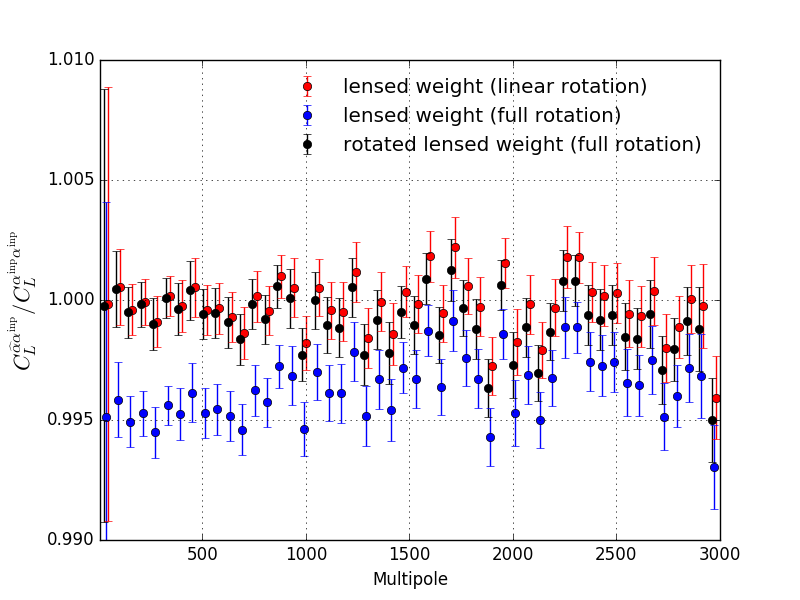
Figure 1: Cross power spectrum between the input and reconstructed cosmic-rotation fluctuations, divided by the input cosmic-rotation spectrum with the Monte Carlo errors (the standard deviation of $100$ realizations divided by $\sqrt{100}$). The rotated CMB map is created according to Eq. (10) (linear) or Eq. (1) (full). The “lensed weight” and “rotated-lensed weight” denote the cases with the lensed and rotated-lensed CMB spectra in the weight function of Eq. (12), respectively.

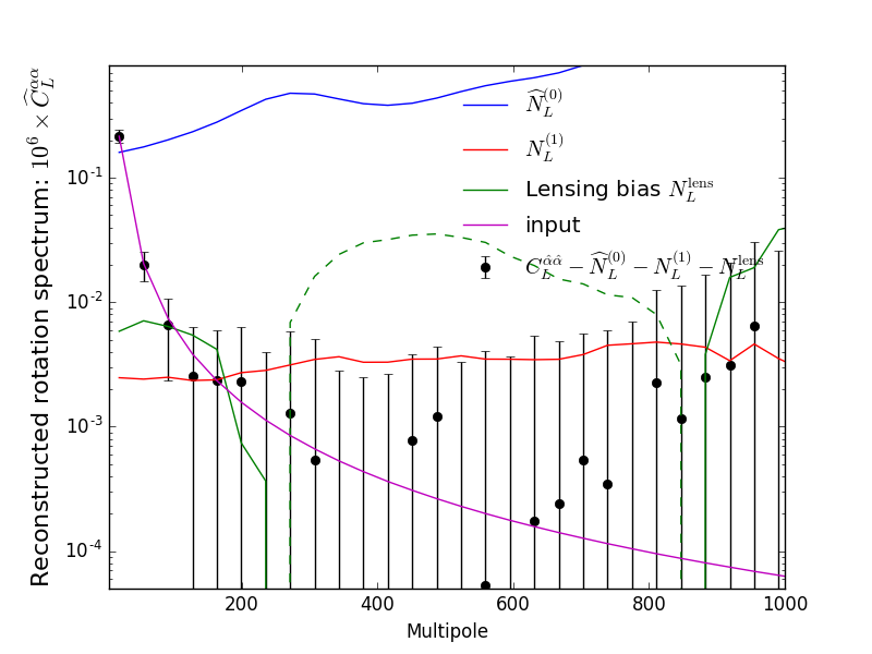
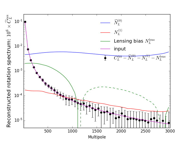
Figure 2: Angular power spectrum of the reconstructed cosmic rotation with subtraction of the disconnected bias, N1 term and lensing bias (black points) with the $1\sigma$ full-sky measured error in the reconstruction for one realization (Left: BK/LiteBIRD–like noise, Right: CMBS4-like noise). We use $100$ realizations of the simulated maps and the Monte Carlo error is $10\%$ of the error bars. We also show the disconnected bias (blue), N1 term (red), lensing bias (green), and the input rotation power spectrum (magenta). The dashed line shows the negative value.

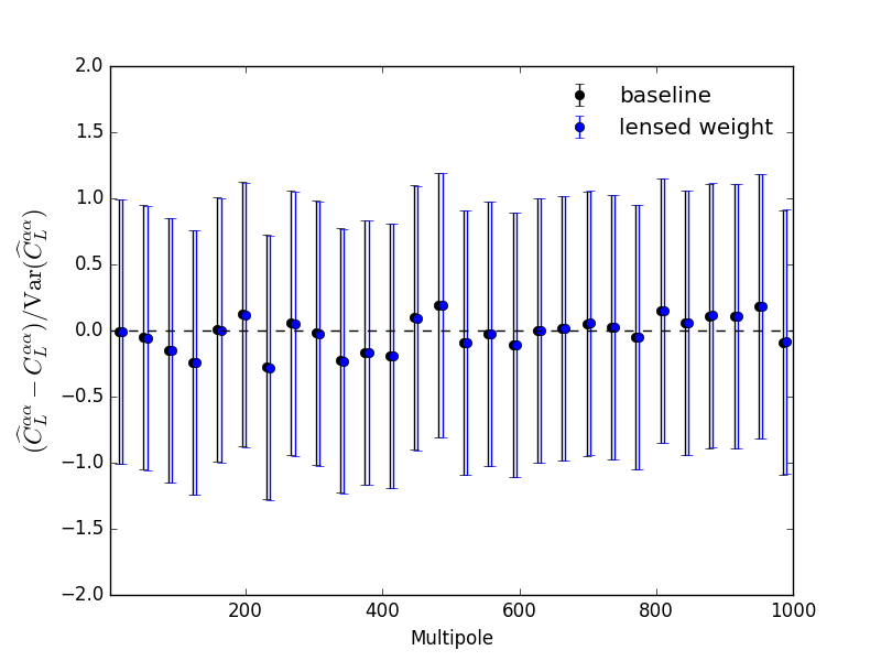
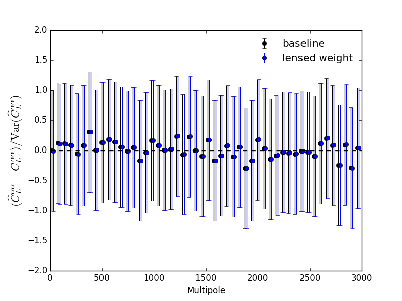
Figure 3: Angular power spectrum of the reconstructed cosmic rotation after the subtraction of the disconnected bias, N1 term, lensing bias and input cosmic-rotation power spectrum (black) with the $1\sigma$ full-sky measured error for one realization (Left: BK/LiteBIRD–like noise, Right: CMBS4-like noise). We use $100$ realizations of the simulated maps and the Monte Carlo error is $10\%$ of the error bars. We also show the case with the lensed CMB power spectrum in the weight function of Eq. (12) (lensed weight).

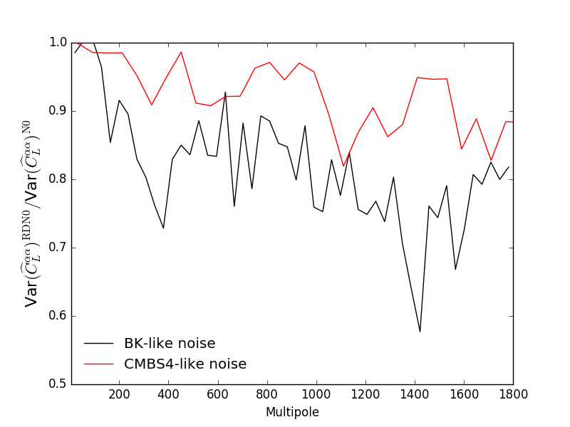
Figure 4: The variance of the reconstructed rotation spectrum with the realization-dependent disconnected bias (RDN0) divided by that with the analytic disconnected bias (N0). We show the cases with the BK/LiteBIRD–like and CMBS4-like noise.

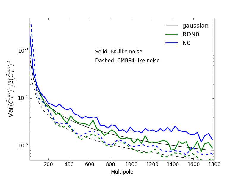
Figure 5: Test of the Gaussian variance. We show the variances of the reconstructed rotation spectrum with the realization-dependent disconnected bias (RDN0) and with the analytic disconnected bias (N0). They are divided by $2(\widehat{C}_{L}^{\alpha\alpha})^{2}$. The black lines show the case when the reconstructed power spectrum is described as a Gaussian statistics. Both the BK/LiteBIRD–like (solid) and CMBS4-like noise cases (dashed) are plotted.

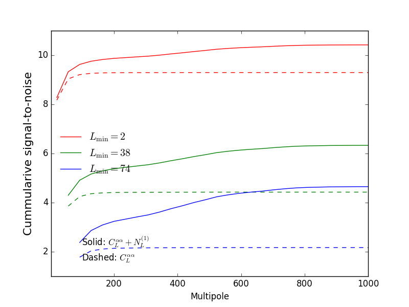
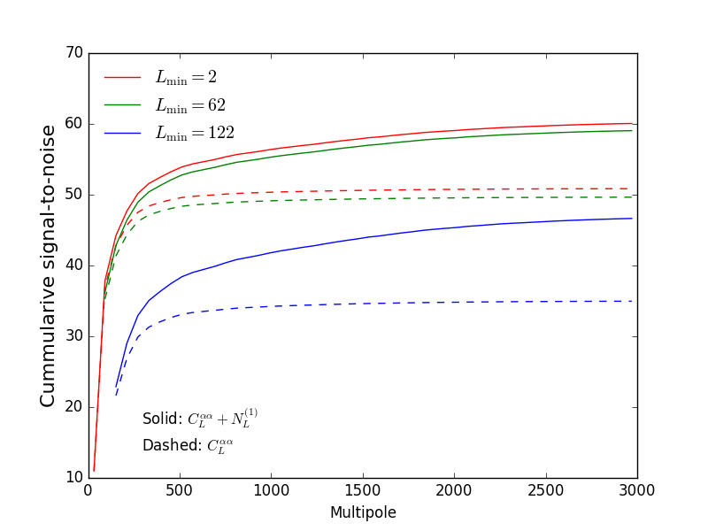
Figure 6: Cumulative signal-to-noise ratio of the cosmic-rotation power spectrum amplitude with and without the N1 term (Left: BK/LiteBIRD-like noise, Right: CMBS4-like noise). We show the cases with different minimum multipole of the rotation spectrum.

We first test the unbiasedness of the cosmic-rotation quadratic estimator given by Eq. (13). The reconstructed cosmic rotation anisotropies are cross-correlated with the input cosmic rotation fluctuations. This cross-power spectrum is then compared with the input cosmic rotation spectrum. The cross spectrum is given analytically by

$$(2\pi)^{2}\delta^{D}_{\bm{0}}C_{L}^{\widehat{\alpha}\alpha} =\int\!\!\frac{\,{\rm d}^{2}\bm{\ell}\,}{(2\pi)^{2}}\,\frac{w^{\alpha}_{\textit{{L}},\bm{\ell}}}{\widehat{C}^{\rm EE}_{\ell}\widehat{C}^{\rm BB}_{|\textit{{L}}-\bm{\ell}|}}\langle\widehat{E}_{\bm{\ell}}\widehat{B}_{\textit{{L}}-\bm{\ell}}\rangle_{\alpha}\alpha_{\textit{{L}}}$$

$$=(2\pi)^{2}\delta^{D}_{\bm{0}}C_{L}^{\alpha\alpha}+\mathcal{O}[(C_{L}^{\alpha\alpha})^{2}]\,.$$ (32)

If the CMB map is rotated by Eq. (10), the above cross spectrum contains up to third order of $\alpha$ and is equivalent to the input spectrum.

Fig. 1 shows the cross power spectrum between reconstructed and input cosmic rotation fluctuations. We show two cases; rotating the polarization map according to Eq. (10) (linear) or Eq. (1) (full). We assume the CMBS4-like noise and use $E$ and $B$ modes up to $\ell=3000$ in the reconstruction. In the linear case, the cross power spectrum is in good agreement with the input spectrum. If the higher order of $\alpha$ is included (full), we find that the cross power spectrum is smaller than the input spectrum at sub-percent level. To reduce the higher-order contributions, we follow the similar treatment of the lensing power reconstruction Lewis et al. (2011); i.e., we use the rotated-lensed power spectrum to the weight function in Eq. (12). The result is shown as “rotated-lensed weight”. The corrected cross-power spectrum becomes close to the input spectrum. As we show below, although the impact of the higher-order rotation on the power spectrum reconstruction is not significant, we use the rotated-lensed power spectrum in the baseline analysis.

III.3.2 Reconstructed power spectrum

Next we discuss the cosmic-rotation power spectrum reconstruction employing the simulated CMB maps described above. We perform the power spectrum reconstruction in the two cases of the instrumental noise specification, i.e., the BK/LiteBIRD–like noise and CMBS4-like noise.

Fig. 2 shows the power spectrum of the reconstructed cosmic rotation after subtracting the disconnected bias, N1 term and lensing bias, i.e.,

$$\widehat{C}_{L}^{\alpha\alpha}=C_{L}^{\widehat{\alpha}\widehat{\alpha}}-N_{L}^{(0)}-N_{L}^{(1)}-N_{L}^{\rm lens}\,.$$ (33)

Here $N_{L}^{\rm lens}$ is the lensing bias. This de-biased power spectrum is in good agreement with the input rotation power spectrum in both the BK/LiteBIRD–like and CMBS4-like noise cases. We also show the significance of the disconnected bias (blue), N1 term (red) and lensing bias (green). The most dominant contribution comes from the disconnected bias. The N1 term dominates over the input rotation spectrum at smaller scales ($L=200$ for the BK/LiteBIRD–like noise and $L=800$ for the CMBS4-like noise). Although the lensing bias is smaller than the disconnected bias in both the BK/LiteBIRD–like and CMBS4-like noise cases, the impact of the lensing bias is significant compared to the error bars. Note that the statistical errors are computed for $200\times 200$ deg², and the impact of the lensing bias is reduced for CMB observations at a small patch of sky (e.g., BK).

Fig. 3 shows difference between the reconstructed power spectrum shown in Fig. 2 and the input cosmic-rotation power spectrum, $\widehat{C}_{L}^{\alpha\alpha}-C_{L}^{\alpha\alpha}$. The difference is consistent with zero within at least sub percent level. This results mean that the reconstructed power spectrum is described by the sum of the disconnected bias, N1 term, lensing bias and the input cosmic-rotation spectrum. We also show that the choice of the weight function does not significantly affect the power spectrum reconstruction, and the reconstructed power spectrum is in good agreement with the sum of the disconnected bias, N1 term, lensing bias and the input cosmic-rotation spectrum. This result implies that, unlike the lensing reconstruction, the higher-order biases such as the “N2 bias” Hanson et al. (2011) is negligible in the experimental specifications considered here.

III.3.3 Realization-dependent disconnected bias and variance

The use of the realization-dependent disconnected bias could reduce the statistical uncertainties of the cosmic rotation power spectrum by suppressing the off-diagonal covariance of the reconstructed rotation power spectrum. Fig. 4 shows the variance in the case with the realization-dependent disconnected bias (RDN0) divided by that with the realization-independent disconnected bias (N0). We show the cases with the BK/LiteBIRD–like noise and CMBS4-like noise. In both cases, using the realization-dependent disconnected bias, the statistical uncertainty of the reconstructed power spectrum decreases and is improved by roughly $10$%–$20$% compared to the case with the disconnected bias estimated from the simulation alone.

Fig. 5 shows a test of the Gaussian variance by plotting the following quantity:

$$N_{b}\equiv\frac{{\rm Var}(\widehat{C}_{b}^{\alpha\alpha})^{2}}{2(\widehat{C}_{b}^{\alpha\alpha})^{2}}\,.$$ (34)

If the reconstructed power spectrum is Gaussian, $N_{b}$ coincides with the number of multipoles at the $b$th bin. We find that the realization-dependent bias reduces the non-Gaussian variance of the reconstructed power spectrum. The variance of the reconstructed power spectrum with the realization-dependent bias is consistent with the Gaussian variance.

III.3.4 Signal-to-noise

Since the N1 term is considered as a signal, here we discuss the benefit of adding the N1 term to constrain the comic rotation. We quantify the impact of the inclusion of the N1 term on the cosmic rotation constraints by the following signal-to-noise ratio:

$$\left(\frac{S}{N}\right)_{<b}=\sqrt{\sum_{b}\frac{(C_{b}^{\alpha\alpha}+N_{b}^{(1)})^{2}}{{\rm Var}(C_{b}^{\widehat{\alpha}\widehat{\alpha}})^{2}}}\,.$$ (35)

Here $b$ denotes the bin center of the multipole binning and Var$(C_{b}^{\widehat{\alpha}\widehat{\alpha}})$ is the variance of the reconstructed rotation spectrum obtained from simulations.

Fig. 6 plots the above signal-to-noise with and without the N1 term. In practice, if CMB data is obtained at some region of sky, CMB analysis is usually performed within the partial sky region and the minimum multipole we can extract is limited. Therefore, we also show the impact of the minimum multipole on the signal-to-noise with varying the minimum multipoles of $C_{b}^{\alpha\alpha}$. Since the cosmic rotation power spectrum becomes large at low multipoles, the signal-to-noise decreases as the minimum multipole becomes large. The impact of the N1 term becomes significant as the minimum multipole increases. The results indicate that, in ongoing and future CMB experiments, to quantify the constraints on the overall amplitude of the cosmic rotation anisotropies, the N1 term is needed to be included.

IV Summary

We have investigated the reconstruction of the cosmic rotation power spectrum from CMB polarization anisotropies, assuming the ongoing and future CMB experiments such as BK, CMBS4, and LiteBIRD. The cosmic rotation power spectrum is assumed to be the scale-invariant spectrum which is motivated by the inflationary origin of the cosmic rotation anisotropies. We found that the N1 term dominates over the original input rotation spectrum at small scales and increases the total signal-to-noise of the amplitudes of the cosmic rotation power spectrum. The lensing bias is significant compared to the statistical error in the case of LiteBIRD and CMBS4, but the impact of the lensing bias becomes negligible for CMB observations at a small patch of sky. The higher-order biases beyond the N1 term is found to be not significant. We showed that the sum of the disconnected bias, N1 term, lensing bias and input rotation spectrum is in good agreement with the power spectrum of the quadratic estimator. We also found that the use of the realization-dependent disconnected bias decreases the statistical uncertainties of the reconstructed rotation power spectrum by $10$%–$20$% depending on experimental specifications.

For high-sensitivity CMB experiments, the lensing $B$ mode degrades the sensitivity to the cosmic rotation Yadav et al. (2009). Since such high-sensitivity experiments can significantly suppress the contributions of the lensing $B$ mode by the so-called delensing technique (e.g., Kesden et al. (2002)). However, the $B$ mode delensing at small scales suffers from the delensing bias Seljak and Hirata (2004), and demonstration of the cosmic rotation reconstruction from the delensed $B$ modes is required. We leave the analysis including the delensing to future work.

Appendix A Disconnected bias estimation

Here we briefly summarize the derivation of the realization-dependent disconnected bias in the case of the cosmic rotation as described in Eq. (27). The derivation is similar to that in the case of the lensing reconstruction which is given in, e.g., the Appendix of Ref. Bicep2 / Keck Array Collaboration (2016).

The disconnected bias of Eq. (27) emerges naturally when deriving the optimal trispectrum estimator from the CMB polarization likelihood. The optimal trispectrum estimator is derived from the Edgeworth expansion of the CMB polarization likelihood;

$$\mathcal{L}\propto\left[\prod_{i=1}^{4}\int\!\!\frac{\,{\rm d}^{2}\bm{\ell}_{i}\,}{(2\pi)^{2}}\,\right]\langle E_{\bm{\ell}_{1}}B_{\bm{\ell}_{2}}E_{\bm{\ell}_{3}}B_{\bm{\ell}_{4}}\rangle_{\rm C}\dfrac{\partial}{\partial E_{\bm{\ell}_{1}}}\dfrac{\partial}{\partial B_{\bm{\ell}_{2}}}\dfrac{\partial}{\partial E_{\bm{\ell}_{3}}}\dfrac{\partial}{\partial B_{\bm{\ell}_{4}}}\mathcal{L}_{\rm g}\,.$$ (36)

Here $\mathcal{L}_{\rm g}$ is the Gaussian likelihood of the $E$ and $B$ mode. The trispectrum induced by the cosmic rotation is given as

$$\langle E_{\bm{\ell}_{1}}B_{\bm{\ell}_{2}}E_{\bm{\ell}_{3}}B_{\bm{\ell}_{4}}\rangle_{\rm C}\propto\delta^{D}_{\bm{\ell}_{1}+\bm{\ell}_{2}+\bm{\ell}_{3}+\bm{\ell}_{4}}[w^{\alpha}_{\bm{\ell}_{1}+\bm{\ell}_{2},\bm{\ell}_{1}}w^{\alpha}_{\bm{\ell}_{3}+\bm{\ell}_{4},\bm{\ell}_{3}}C_{|\bm{\ell}_{1}+\bm{\ell}_{2}|}^{\alpha\alpha}+w^{\alpha}_{\bm{\ell}_{1}+\bm{\ell}_{4},\bm{\ell}_{1}}w^{\alpha}_{\bm{\ell}_{2}+\bm{\ell}_{3},\bm{\ell}_{2}}C_{|\bm{\ell}_{1}+\bm{\ell}_{4}|}^{\alpha\alpha}]\,,$$ (37)

where $w^{\alpha}_{\textit{{L}},\bm{\ell}}$ is defined in Eq. (12). The approximate formula of the estimator which is numerically tractable is proportional to the derivative of the log-likelihood with respect to $C_{L}^{\alpha\alpha}$. The derivative is given by

$$\dfrac{\partial\mathcal{L}}{\partial C^{\alpha\alpha}_{L}}\propto\left[\prod_{i=1}^{2}\int\!\!\frac{\,{\rm d}^{2}\bm{\ell}_{i}\,}{(2\pi)^{2}}\,\right]w^{\alpha}_{\textit{{L}},\bm{\ell}_{1}}w^{\alpha}_{-\textit{{L}},\bm{\ell}_{2}}\dfrac{\partial}{\partial E_{\bm{\ell}_{1}}}\dfrac{\partial}{\partial B_{\textit{{L}}-\bm{\ell}_{1}}}\dfrac{\partial}{\partial E_{\bm{\ell}_{2}}}\dfrac{\partial}{\partial B_{-\textit{{L}}-\bm{\ell}_{2}}}\mathcal{L}_{\rm g}\simeq\left(|\overline{\alpha}^{EB}_{\textit{{L}}}|^{2}-\frac{\widehat{N}^{\alpha}_{\textit{{L}}}}{(A^{\alpha}_{\textit{{L}}})^{2}}\right)\mathcal{L}_{\rm g}\,.$$ (38)

After correcting the normalization, the above equations leads to an approximate formula of the optimal estimator for $C_{L}^{\alpha\alpha}$ with the subtraction of the disconnected bias.

References

- Bicep2 / Keck Array Collaboration (2015) Bicep2 / Keck Array Collaboration, Phys. Rev. Lett. 116, 031302 (2015), eprint 1510.09217.
- Carroll (1998) S. M. Carroll, Phys. Rev. Lett. 81, 3067 (1998), eprint astro-ph/9806099.
- Pospelov et al. (2009) M. Pospelov, A. Ritz, and C. Skordis, Phys. Rev. Lett. 103, 051302 (2009), eprint 0808.0673.
- Finelli and Galaverni (2009) F. Finelli and M. Galaverni, Phys. Rev. D 79, 063002 (2009), eprint 0802.4210.
- Shiraishi et al. (2016) M. Shiraishi, C. Hikage, R. Nambda, T. Namikawa, and M. Hazumi, Phys. Rev. D 94, 043506 (2016), eprint 1606.06082.
- Marsh (2016) D. J. E. Marsh, Phys. Rep. 643, 1 (2016), eprint 1510.07633.
- Kamionkowski (2010) M. Kamionkowski, Phys. Rev. D 82, 047302 (2010), eprint 1004.3544.
- Caldwell et al. (2011) R. R. Caldwell, V. Gluscevic, and M. Kamionkowski, Phys. Rev. D 84, 043504 (2011), eprint 1104.1634.
- Gluscevic et al. (2013) V. Gluscevic, M. Kamionkowski, and D. Hanson, Phys. Rev. D 87, 047303 (2013), eprint 1210.5507.
- Kosowsky and Loeb (1996) A. Kosowsky and A. Loeb, Astrophys. J. 469, 1 (1996), eprint astro-ph/9601055.
- Harari et al. (1997) D. D. Harari, J. D. Hayward, and M. Zaldarriaga, Phys. Rev. D 55, 1841 (1997), eprint astro-ph/9608098.
- Shaw and Lewis (2010) J. R. Shaw and A. Lewis, Phys. Rev. D 81, 043517 (2010), eprint 0911.2714.
- Yadav et al. (2012a) A. Yadav, L. Pogosian, and T. Vachaspati, Phys. Rev. D 86, 123009 (2012a), eprint 1207.3356.
- Pogosian (2014) L. Pogosian, Mon. Not. R. Astron. Soc. 438, 2508 (2014), eprint 1311.2926.
- Leon et al. (2017) D. Leon, J. Kaufman, B. Keating, and M. Mewes, Mod. Phys. Lett. A 32, 1730002 (2017), eprint 1611.00418.
- Gluscevic et al. (2009) V. Gluscevic, M. Kamionkowski, and A. Cooray, Phys. Rev. D 80, 023510 (2009), eprint 0905.1687.
- Lue et al. (1999) A. Lue, L. Wang, and M. Kamionkowski, Phys. Rev. Lett. 83, 1506 (1999), eprint astro-ph/9812088.
- Kamionkowski (2009) M. Kamionkowski, Phys. Rev. Lett. 102, 111302 (2009), eprint 0810.1286.
- G. Hinshaw et al. (2013) (WMAP Collaboration) G. Hinshaw et al. (WMAP Collaboration), Astrophys. J. 208, 19 (2013), eprint 1212.5226.
- Planck Collaboration (2016) Planck Collaboration, Astron. Astrophys. 596, A13 (2016), eprint 1605.08633.
- Liu and Ng (2017) G.-C. Liu and K.-W. Ng, Phys. Dark Univ. 16, 22 (2017), eprint 1612.02104.
- POLARBEAR Collaboration (2015) POLARBEAR Collaboration, Phys. Rev. D 92, 123509 (2015), eprint 1509.02461.
- Grayson and others (BICEP3 Collaboration) J. A. Grayson and others (BICEP3 Collaboration), Proc. SPIE Int. Soc. Opt. Eng. 9914, 99140S (2016), eprint 1607.04668.
- Matsumura et al. (2014) T. Matsumura et al., J. Low. Temp. Phys. 176, 733 (2014), eprint astro-ph/1311.2847.
- Yadav et al. (2009) A. Yadav, R. Biswas, M. Su, and M. Zaldarriaga, Phys. Rev. D 79, 123009 (2009), eprint 0902.4466.
- Planck Collaboration (2016) Planck Collaboration, Astron. Astrophys. 594, A13 (2016), eprint 1502.01589.
- Pogosian et al. (2011) L. Pogosian, P. S. A. Yadav, Y.-F. Ng, and T. Vachaspati, Phys. Rev. D 84, 043530 (2011), eprint 1106.1438.
- De et al. (2013) S. De, L. Pogosian, and T. Vachaspati, Phys. Rev. D 88, 063527 (2013), eprint 1305.7225.
- Yadav et al. (2012b) A. P. S. Yadav, M. Shimon, and B. G. Keating, Phys. Rev. D 86, 083002 (2012b), eprint 1010.1957.
- Namikawa et al. (2013) T. Namikawa, D. Hanson, and R. Takahashi, Mon. Not. R. Astron. Soc. 431, 609 (2013), eprint 1209.0091.
- Hanson et al. (2011) D. Hanson, A. Challinor, G. Efstathiou, and P. Bielewicz, Phys. Rev. D 83, 043005 (2011), eprint 1008.4403.
- Kesden et al. (2003) M. H. Kesden, A. Cooray, and M. Kamionkowski, Phys. Rev. D 67, 123507 (2003), eprint astro-ph/0302536.
- Hanson et al. (2009) D. Hanson, G. Rocha, and K. Gorski, Mon. Not. R. Astron. Soc. 400, 2169 (2009), eprint 0907.1927.
- Lewis et al. (2000) A. Lewis, A. Challinor, and A. Lasenby, Astrophys. J. 538, 473 (2000), eprint astro-ph/9911177.
- Louis et al. (2013) T. Louis, S. Naess, S. Das, J. Dunkeley, and B. Sherwin, Mon. Not. R. Astron. Soc. 435, 2040 (2013), eprint 1306.6692.
- Knox (1999) L. Knox, Phys. Rev. D 60, 103516 (1999), eprint astro-ph/9902046.
- Lewis et al. (2011) A. Lewis, A. Challinor, and D. Hanson, J. Cosmol. Astropart. Phys. 03, 018 (2011), eprint 1101.2234.
- Kesden et al. (2002) M. Kesden, A. Cooray, and M. Kamionkowski, Phys. Rev. Lett. 89, 011304 (2002), eprint astro-ph/0202434.
- Seljak and Hirata (2004) U. Seljak and C. M. Hirata, Phys. Rev. D 69, 043005 (2004), eprint astro-ph/0310163.
- Bicep2 / Keck Array Collaboration (2016) Bicep2 / Keck Array Collaboration, Astrophys. J. 833, 228 (2016), eprint 1606.01968.