Milne’s Equation revisited: Exact Asymptotic Solutions

Abstract

We present novel approaches for solving Milne’s equation, which was introduced in 1930 as an efficient numerical scheme for the Schrödinger equation. Milne’s equation appears in a wide class of physical problems, ranging from astrophysics and cosmology, to quantum mechanics and quantum optics. We show how a third order linear differential equation is equivalent to Milne’s non-linear equation, and can be used to accurately calculate Milne’s amplitude and phase functions. We also introduce optimization schemes to achieve a convenient, fast, and accurate computation of wave functions using an economical parametrization. These new optimization procedures answer the long standing question of finding non-oscillatory solutions of Milne’s equation. We apply them to long-range potentials and find numerically exact asymptotic solutions.

In 1930, Milne introduced a phase-amplitude approach Milne (1930) for tackling time-independent wave equations. The resulting equation for the amplitude $y(x)$, known as Milne’s equation, is a nonlinear differential equation of second order,

$$\partial_{x}^{2}y=U(x)y+\frac{q^{2}}{y^{3}},$$ (1)

where $U(x)$ is a function of the independent variable $x$, and $q$ is a constant. Replacing a linear wave equation with a nonlinear one for the amplitude is a price worth paying, as Milne’s approach can yield a very economical parametrization of highly oscillating wave functions. In addition, Eq. (1) allows for novel formalistic approaches, and is now used in many areas in physics, as well as being investigated for its mathematical properties Schief (1997).

In astrophysics, studies of stellar equilibrium for white dwarfs or neutron stars employ certain transformations to rewrite the Tolman-Oppenheimer-Volkoff equations in the form of Milne’s equation, which is more amenable for analyzing the stability of stellar objects Kaushal (1998). Milne’s equation is also used in scalar field cosmologies for deriving exact cosmological models Hawkins and Lidsey (2002), for establishing a dynamical correspondence between certain types of cosmologies and quasi-two-dimensional BEC Lidsey (2004), or to investigate the quantum effects of relic gravitons Bakke et al. (2009). Also, the problem of the quantized motion for free fall in a gravitational potential Rosu (2002) has been investigated using Milne’s equation. Moreover, Milne’s approach is used in conjunction with a simple gauge model for studying bilayer graphene Khmelnytskaya and Rosu (2008). Recent work on Berry’s phase in arbitrary dimensions Thilagam (2010), as well as studies of the propagation of quantized electromagnetic waves through nondispersive media de Lima et al. (2009); Pedrosa (2011) also make use of Milne’s equation.

In this Letter, we consider the original problem that led Milne to develop his equation, namely the one-dimensional differential equation,

$$\psi^{\prime\prime}(x)-U(x)\psi(x)=0.$$ (2)

By using two linearly independent solutions $u(x)$ and $v(x)$ of Eq. (2), and defining the function $y(x)=\sqrt{u^{2}+v^{2}}$, Milne showed Milne (1930) that Eq. (2) leads to the differential equation (1) where the constant $q=u^{\prime}v-uv^{\prime}$ is the Wronskian of $u$ and $v$. We emphasize that, assuming $q\neq 0$, any particular solution $y(x)$ of Eq. (1) can be used to construct the most general solution of Eq. (2) via the simple parametrization,

$$\psi(x)=Cy(x)\sin\left[\theta(x)-\theta_{0}\right],\quad\theta(x)=q\!\int_{x_{0}}^{x}\frac{d\tau}{y^{2}(\tau)},\\$$ (3)

where $C$ and $\theta_{0}$ are arbitrary constants.

Milne’s phase-amplitude method has been used extensively in atomic and molecular physics problems and also in physical chemistry Yuan and Light (1974); Lee and Light (1974). It is especially suitable in the multi-channel quantum defect theory framework Mies and Raoult (2000); Osséni et al. (2009); Yoo and Greene (1986a); Burke et al. (1998); Bohn (1994); Idziaszek et al. (2011); Bohn and Julienne (1999) because it makes it possible to construct optimal reference functions. We note that this simple parametrization of the wave function has been employed in other approaches, e.g., the WKB approximation and the variable phase method Calogero (1967). The latter is an exact approach, as is Milne’s. However, Milne’s approach is more advantageous, e.g., in the context of quantum defect theory, see Greene et al. Greene et al. (1982).

Although Milne’s method is very appealing, it presents some challenges. First, Eq. (1) is obviously nonlinear, though tractable numerically. Second, a more serious difficulty is finding the elusive optimally smooth solution among the infinite number of oscillatory solutions of Eq. (1), which was the original goal of Milne, i.e., replacing a rapidly oscillating wave function $\psi(x)$ by two slowly varying functions $y(x)$ and $\theta(x)$. As mentioned above, any solution $y(x)$ and its associated phase $\theta(x)$ can be used in Eq. (3) to parametrize $\psi(x)$, but an oscillatory behavior of $y(x)$ would render this approach inconvenient and computationally expensive. Numerous attempts have been made to find the optimal solution for Milne’s equation, yet they are either insufficiently optimal due to reliance on the WKB approximation Greene et al. (1982); Jungen et al. (2000); Sidky (2000), not robust enough with respect to iterations of WKB Seaton and Peach (1962); Rawitscher (2015), or not general enough Matzkin (2000). In the remainder of the Letter, we present two novel optimization schemes which are efficient, convenient, accurate, and general.

Linear differential equation for the envelope — To remove the non-linear term in Milne’s equation, we introduce a new quantity, namely $\rho(x)\equiv y^{2}(x)$, which we refer to as the envelope function. Simply substituting $y=\sqrt{\rho}$ in Eq. (1), we obtain

$$\rho^{\prime\prime}-2U\rho-\frac{2}{\rho}\left[q^{2}+\frac{1}{4}\left(\rho^{\prime}\right)^{2}\right]=0\;.$$ (4)

Next, we multiply Eq. (4) with $\rho$ and take the derivative Kiyokawa (2015); Schief (1997); Olver and Maximon (2010), yielding

$$\rho^{\prime\prime\prime}-4U\rho^{\prime}-2U^{\prime}\rho=0\;,$$ (5)

which is a linear differential equation, albeit of third order. We emphasize that, despite the obvious advantages of replacing Milne’s nonlinear equation (1) with the linear equation (5), difficulties in finding the non-oscillatory envelope persist. Thus, an optimization procedure is needed to isolate the smooth solution, which will provide the initial conditions of Eq. (5) for propagating $\rho(x)$ along the $x$-axis, with a numerical solver employing a spectral integration method based on Chebyshev polynomials El-gendi (1969); Greengard (1991); Mihaila and Mihaila (2002).

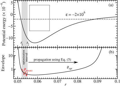
Figure 1: (a) Potential energy, Eq. (9), used for optimization. Rectangle corresponds the ranges of $r$ and $\varepsilon$ in Fig. 2. Shaded area marks the optimization interval. (b) Red line for $\rho_{\mathrm{ansatz}}=\phi^{2}+\chi^{2}$, corresponding to $A=B=1,\,C=0$, and black line for $\rho_{\mathrm{opt}}=A\phi^{2}+B\chi^{2}+2C\phi\chi$ with $A=0.8533850906254,\,B=1.245534003812,\,C=-0.2508388899674$, which was propagated outside the optimization interval using Eq. (5).

Optimization — We now introduce a simple optimization method for finding the smooth envelope in any classically allowed region. First we note that the solutions $u$ and $v$ in the original expression $y=\sqrt{u^{2}+v^{2}}$ can each be written as superpositions of other independent solutions $\phi(x)$ and $\chi(x)$, i.e., $u=a\phi+b\chi$ and $v=\alpha\phi+\beta\chi$. Thus we obtain

$$\rho=A\phi^{2}+B\chi^{2}+2C\phi\chi\;,$$ (6)

with $A=a^{2}+\alpha^{2}$, $B=b^{2}+\beta^{2}$, and $C=ab+\alpha\beta$. Similarly, the Wronskian $q=u^{\prime}v-uv^{\prime}$ yields

$$q^{2}=(\phi\chi^{\prime}-\chi\phi^{\prime})^{2}(AB-C^{2})\;.$$ (7)

If $\phi$ and $\chi$ are two linearly independent solutions of Eq. (2), it can be shown that $\phi^{2}$, $\chi^{2}$, and $\phi\chi$ are three linearly independent solutions of Eq. (5). Thus, if $A,\,B,\,C$ are regarded as arbitrary constants, Eq. (6) represents the most general solution of Eq. (5).

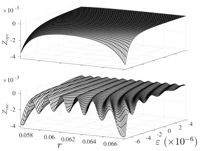
Figure 2: $Z(\varepsilon,r)$ using optimization (upper) and using the WKB-initialization (lower). See text for details. The range of the surface plot corresponds to the rectangle in Fig. 1a.

We first compute two linearly independent solutions $\phi$ and $\chi$ of Eq. (2) within a narrow interval $[x_{1},x_{2}]$ inside a classically allowed region. Note that, for the optimization to be effective, the interval $[x_{1},x_{2}]$ should cover one or two oscillations of $\phi$ and $\chi$. Moreover, by computing $\phi(x)$ and $\chi(x)$ with high accuracy, we ensure that $\rho(x)$ in Eq. (6) is numerically exact within $[x_{1},x_{2}]$, and we label it $\rho_{\rm exact}(x)$. We emphasize that for arbitrary parameters $A,\,B,\,C$, the envelope will be oscillatory. Next, we expand the exact envelope over the interval $[x_{1},x_{2}]$ in a small polynomial basis of size $N\lessapprox 20$, such that it cannot reproduce the oscillations of $\rho_{\rm exact}$, in effect downgrading it to an approximate envelope, $\rho_{\mathrm{approx}}$. For arbitrary parameters $(A,B,C)$, the latter will be a poor approximation, i.e., the error $\delta\rho=\lVert\rho_{\mathrm{exact}}-\rho_{\mathrm{approx}}\rVert$ will be large. However, when the parameters are precisely optimized such that the envelope has a non-oscillatory behavior, the error $\delta\rho$ vanishes because the small basis is sufficient to accurately reproduce the smooth envelope. A standard optimization subroutine is used to minimize the error function,

$$\delta\rho\equiv\underset{x\in[x_{1},x_{2}]}{\rm max}\big{|}\rho_{\rm exact}(Q;x)-\rho_{\mathrm{approx}}(Q;x)\big{|},$$ (8)

over the parameter space $Q\equiv(A,\,B,\,C|q)$. We remark that Eq. (7) represents a constraint for $A,\,B,\,C$, because $q$ is assumed fixed, and thus the parameter space $Q\equiv(A,\,B,\,C|q)$ is only two dimensional. Our implementation uses Chebyshev polynomials, $T_{n}(x)=\cos[n\,\mathrm{acos}(x)]$, for the interpolation $\rho_{\mathrm{approx}}=\sum_{n=0}^{N-1}c_{n}(Q)T_{n}(x)$. The optimized (smooth) envelope is then used as an initial condition for Eq. (5), and $\rho(x)$ is propagated on both sides of the initial working interval, to cover the entire $x$-domain.

As a first application, we consider the time-independent radial Schrödinger equation (2), with $0<x<\infty$ and $U(x)=\frac{2\mu}{\hbar^{2}}[V(x)-E]+\ell(\ell+1)/x^{2}$, where $\mu$ is the reduced mass, $V(x)$ the interaction potential, and $\ell(\ell+1)/x^{2}$ the centrifugal term for a given partial wave $\ell$. To simplify notations, we use dimensionless quantities, $r=x/x_{s}$ and $\varepsilon=E/E_{s}$ with $E_{s}=\hbar/2\mu x_{s}^{2}$. The length scale $x_{s}$ and the energy scale $E_{s}$ can be chosen arbitrarily, but for a potential with power-law tail $V(x)\sim C_{n}x^{-n}$, the van der Waals units with $x_{s}=(2\mu|C_{n}|/\hbar^{2})^{\frac{1}{n-2}}$ are most convenient. Thus, for the remainder of this Letter, we redefine $x_{s}^{2}U(x)\to U(r)$ such that it is dimensionless. As an illustrative example, we use $U(r)=-\varepsilon+V(r)$ with

$$V(r)=-\frac{1}{r^{6}}+V_{0}e^{-\gamma r},$$ (9)

where $V_{0}=1.55\times 10^{12}$ and $\gamma=200$, which mimics the a${}^{3}\Sigma_{u}^{+}$ potential curve for Cs₂. The shaded area in Fig. 1a between $r_{1}=0.052$ and $r_{2}=0.055$ marks the optimization interval for $\varepsilon=-2\times 10^{6}$. The solutions $\phi$ and $\chi$ are initialized at $r_{1}$ with $\phi=0,\ \phi^{\prime}=k_{1}=\sqrt{-U(r_{1})}$ and $\chi=1,\ \chi^{\prime}=0$, such that $\phi$ and $\chi$ are similar to sine and cosine respectively. Thus a good choice for the initial ansatz is $\rho_{\mathrm{ansatz}}=\phi^{2}+\chi^{2}$, shown as the oscillatory red curve in Fig. 1b. Finally, we minimize $\delta\rho$ and find the optimal values for $A,B,C$ which give the smooth envelope $\rho_{\mathrm{opt}}(r)$ shown as the black curve in Fig. 1b. We emphasize that this procedure is very robust with respect to the size of the optimization interval; namely, we obtain the same values of $A,B,C$, when the interval is enlarged to contain up to three oscillations.

Figure 2 compares our optimization procedure with the standard WKB-initialized scheme Yoo and Greene (1986b), which relies on using the WKB approximation to impose the initial condition for $\rho$ at the bottom of the potential ($r_{0}\approx 0.05856$). We use Eq. (5) to compute both the optimal envelope, $\rho_{\mathrm{opt}}(x)$, and WKB-initialized envelope denoted as $\rho_{\mathrm{osc}}(x)$ for a range of energies corresponding to $-7\times 10^{6}<\varepsilon<4\times 10^{6}$. For clarity, we make use of the WKB approximation $\rho_{\mathrm{wkb}}(r)\equiv q|U(r)|^{-1/2}$ to rescale both $\rho_{\mathrm{opt}}(r)$ and $\rho_{\mathrm{osc}}(r)$. Thus, we define $Z_{\mathrm{opt}}$ and $Z_{\mathrm{osc}}$ according to $Z(\varepsilon,r)=\frac{\rho(r)}{\rho_{\mathrm{wkb}}(r)}-1$, and plot them in Fig. 2. Note the oscillatory behavior of $Z_{\mathrm{osc}}$, while $Z_{\mathrm{opt}}$ obtained using our $\rho_{\mathrm{opt}}(r)$ is smooth.

The optimization method described above is applicable for all classically allowed regions, and it provides a smooth envelope which can be propagated efficiently by solving Eq. (5). Note that when the propagation enters a classically forbidden region, the envelope will take on an increasing behavior, e.g., for $\varepsilon=-\kappa^{2}<0$ and $r\to\infty$, $y(r)\sim e^{\kappa r}$. Thus, the solution $\psi=y(r)\sin\theta(r)$, with $\theta(r)=q\int_{0}^{r}\frac{d\tau}{\rho(\tau)}$, will diverge when $r\to\infty$, unless $\theta(\infty)$ is an integer number of $\pi$, in which case, $\sin\theta(r)\sim e^{-2\kappa r}$ guarantees that $\psi$ has the correct behavior of an eigenfunction corresponding to a bound state. However, for scattering solutions ($\varepsilon>0$), the asymptotic region ($r\to\infty$) can be tackled even more directly, as we show next.

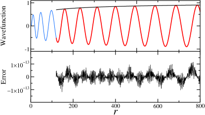
Figure 3: Accuracy test for an attractive Coulomb potential. Upper: blue line for $F_{\ell}$ computed using the radial equation (2); red line for $F_{\ell}$ obtained from the envelope $\rho$ computed using Eqs. (10) and (5); black line for the amplitude $y=\sqrt{\rho}$. Lower: the difference between the red and blue curves. See text for details.

Exact asymptotic solutions for scattering — For $E>0$, the usual numerical approach for the radial Schrödinger equation consists in propagating its solution far into the asymptotic region, where matching is performed using Bessel or Coulomb functions, and the S-matrix is extracted. Here we present a novel approach based on the phase-envelope method for efficiently computing highly accurate asymptotic solutions for any potential $V(r)$ which may contain Coulomb and centrifugal terms. First, the change of variable $z=1/r$ maps the infinite radial interval $[r_{\mathrm{max}},\infty]$ into a finite interval $[0,z_{\mathrm{max}}]$ with $z_{\mathrm{max}}=1/r_{\mathrm{max}}$, thus making it possible to enforce boundary conditions at $r=\infty$ ($z=0$) and to account for the entire tail of $V(r)$ without approximations. Secondly, the linear equation (5) allows for a simple implementation of a spectral integration method employing a small number of Chebyshev polynomials Greengard (1991); Mihaila and Mihaila (2002), which yields a highly accurate envelope. Rewriting Eq. (5) in the new variable $z$, we have

$$z^{4}\partial_{z}^{3}\rho+6z^{3}\partial_{z}^{2}\rho+6z^{2}\partial_{z}\rho-4U\partial_{z}\rho-2(\partial_{z}U)\rho=0.$$ (10)

Next, in order to impose the initial condition $\rho|_{z=0}=1$, Eq. (10) is integrated only one time, and the smooth envelope $\rho_{\infty}(z)$ is extracted as a unique solution of the newly obtained equation, without the need for an explicit optimization. Indeed, all other possible solutions of Eq. (10) oscillate infinitely fast near $z=0$ ($r=\infty$), and thus they exist outside the small subspace spanned by the Chebyshev basis, which is restricted to polynomials of degree $N\leq 20$. The use of a small basis is of critical importance, as it ensures a very effective suppression of oscillatory behavior, while it is nevertheless sufficient for a highly accurate smooth solution.

As an illustrative example, we use an attractive Coulomb potential with partial wave $\ell=2$ and $k=\sqrt{\varepsilon}=0.05$, specifically, $U(r)=-1/r+6/r^{2}-k^{2}$. For a Coulomb potential, it is well known that the asymptotic phase also contains a logarithmic term, which we separate explicitly: $\theta_{\infty}(r)=kr+\frac{\ln(2kr)}{2k}-\frac{\ell}{2}\pi+\tilde{\theta}(r)$. Correspondingly, it is necessary to decompose the envelope as $\rho_{\infty}(z)=1-\frac{z}{2k^{2}}+u(z)$. Hence the nontrivial phase $\tilde{\theta}$ reads

$$\tilde{\theta}(z)=k\int_{0}^{z}\frac{d\tau}{\tau^{2}}\frac{1}{\rho(\tau)}\left[u(\tau)+\frac{\tau}{2k^{2}}\left(u(\tau)-\frac{\tau}{2k^{2}}\right)\right],$$ (11)

which is computed using the Clenshaw–Curtis quadrature Clenshaw and Curtis (1960). Note that we used $q=k$ in Eq. (11).

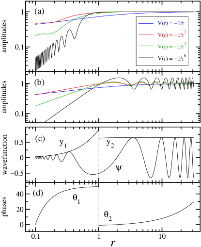
Figure 4: (a) Asymptotically optimized amplitudes for $\varepsilon=1$ and $V(r)=-1/r^{n}$, with $n=1,3,4,6$. (b) Amplitudes optimized at short range for the same cases. (c) Regular solution $\psi=y_{1}\sin\theta_{1}=y_{2}\sin\theta_{2}$ for $V(r)=-1/r^{6}$. (d) Phases $\theta_{1,2}$ corresponding to amplitudes $y_{1,2}$. See text for details.

We emphasize that accurate solutions for the envelope and phase can be obtained in the interval $[0,z_{\mathrm{max}}]$ without the need to further subdivide it into smaller sectors. Subsequently, it is convenient to revert to the original variable $r$, and then propagate the asymptotic envelope and phase inwards, from $r_{\mathrm{max}}$ to $r=0$, according to Eqs. (5) and (3). The amplitude $y_{\infty}(r)=\sqrt{\rho_{\infty}(r)}$ and the phase $\theta_{\infty}(r)$ can now be used to construct any solution of the radial Schrödinger equation. In particular, the regular solution obtained from the phase-envelope method can be compared with its version computed independently as a solution of Eq. (2). The former is expressed as $F_{\ell}(q,r)=y_{\infty}\sin(\theta_{\infty}+\sigma_{\ell})$, where $\sigma_{\ell}$ is the Coulomb phase shift, while the latter is initialized at $r=0$ with the appropriate behavior, $F_{\ell}\sim r^{\ell+1}$, and a suitable normalization factor Seaton and Peach (1962); Rawitscher (2015), and then it is propagated outwards. As shown in Fig. 3, the two independently computed wavefunctions agree to thirteen digits, nearly the full fifteen digits available in standard double-precision computer arithmetic. We emphasize that, apart from the appropriate factors used to initialize the solutions of Eqs. (2) and (10), no rescaling of the wavefunctions was necessary for the comparison in Fig. 3.

Combining locally optimized solutions — When two classically allowed regions are separated by a classically forbidden region due to a barrier, it is well known Lee and Light (1974) that a global envelope which is smooth in all regions cannot exist. In fact, this lack of global smoothness can also manifest within a single classically allowed region. Indeed, when the asymptotically optimized envelope is propagated inwards, it may develop oscillations at short range, as shown in Fig. 4a. Conversely, if the envelope is first optimized at short range, it may develop oscillations when propagated outwards into the asymptotic region, see Fig. 4b. This type of oscillatory behavior is directly related to quantum reflectionFriedrich and Jurisch (2004); Côté et al. (1997); Segev et al. (1997); Côté et al. (1998); Côté and Segev (2003); Kallush et al. (2005), which is very pronounced at low energy, but diminishes and eventually disappears at high energy. The results shown in Figs. 4(a) and (b) correspond to $\ell=0$ and $V(r)=-\frac{1}{r^{n}}$ with $n=1,3,4,6$. Note that the oscillations are more pronounced for high $n$, due to the more abrupt behavior of $V(r)$, while $n=1$ (Coulomb) is a special case which admits a globally smooth envelope for all energies.

In the absence of a globally smooth envelope, a simple partitioning scheme can be used to take advantage of regionally smooth phases and envelopes. To illustrate such an approach, we use $V(r)=-1/r^{6}$ with $\ell=0$ and $\varepsilon=1$. In the first region ($r\leq 1$) we employ the short range optimization to obtain $\psi=y_{1}\sin\theta_{1}$, with $\theta_{1}=0$ at $r_{0}=0.1$, where we placed a hard wall. In the asymptotic region ($r\geq 1$) we construct the solution $\psi=y_{2}\sin\theta_{2}$ with $y_{2}=cy_{\mathrm{\infty}}$ and $\theta_{2}=\theta_{\infty}+\delta$. Matching for $\psi$ and $\psi^{\prime}$ is imposed at $r=1$ to determine $c$ and $\delta$. The amplitudes $y_{1}(r)$ and $y_{2}(r)$ are shown in Fig. 4c and the phases $\theta_{1}(r)$ and $\theta_{2}(r)$ are shown in Fig. 4d. Note that $\theta^{\prime}_{1}\neq\theta^{\prime}_{2}$ and $\theta_{1}\neq\theta_{2}$ (mod $\pi$) at $r=1$. Thus, despite quantum reflection, any wavefunction $\psi(r)$ can still be parametrized economically by judiciously partitioning the $r$ domain and computing separately a smooth envelope and the corresponding phase for each region.

Conclusions — In this Letter, we derived a linear alternative, Eq. (5), to Milne’s nonlinear equation, and presented new approaches for solving Milne’s amplitude equation. For short and medium range, we developed a simple and practical recipe for optimization which provides a smooth envelope. For $E>0$ the non-oscillatory envelope and phase can be computed very easily for the entire asymptotic region for any type of potential. In turn, the optimized envelope allows for the computation of quantities which have a smooth energy dependence. We also showed that very high numerical precision can be obtained in a straightforward manner using the prescribed approaches. Finally, extension of this method to coupled channel problems is underway, where the applicability of Chebyshev-based solvers using the mapping $z=\frac{1}{r}$, is explored.

This work was partially supported by the MURI US Army Research Office Grant No. W911NF-14-1-0378 (IS) and by the US Army Research Office, Chemistry Division, Grant No. W911NF-13-1-0213 (DS and RC).

References

- Milne (1930) W. E. Milne, Phys. Rev. 35, 863 (1930), URL http://link.aps.org/doi/10.1103/PhysRev.35.863.
- Schief (1997) W. Schief, Appl. Math. Lett. 10, 13 (1997), URL http://www.sciencedirect.com/science/article/pii/S0893965997000268.
- Kaushal (1998) R. Kaushal, Class. Quantum Grav. 15, 197 (1998).
- Hawkins and Lidsey (2002) R. M. Hawkins and J. E. Lidsey, Phys. Rev. D 66, 023523 (2002), URL http://link.aps.org/doi/10.1103/PhysRevD.66.023523.
- Lidsey (2004) J. E. Lidsey, Class. Quantum Grav. 21, 777 (2004), URL http://stacks.iop.org/0264-9381/21/i=4/a=002.
- Bakke et al. (2009) K. Bakke, I. Pedrosa, and C. Furtado, J. Math. Phys. 50, 113521 (2009).
- Rosu (2002) H. C. Rosu, Phys. Scr. 65, 296 (2002), URL http://stacks.iop.org/1402-4896/65/i=4/a=002.
- Khmelnytskaya and Rosu (2008) K. V. Khmelnytskaya and H. C. Rosu, J. Phys. A 42, 042004 (2008).
- Thilagam (2010) A. Thilagam, J. Phys. A 43, 354004 (2010), URL http://stacks.iop.org/1751-8121/43/i=35/a=354004.
- de Lima et al. (2009) A. L. de Lima, A. Rosas, and I. Pedrosa, J. Mod. Opt. 56, 41 (2009), URL http://dx.doi.org/10.1080/09500340802428348.
- Pedrosa (2011) I. A. Pedrosa, Phys. Rev. A 83, 032108 (2011), URL http://link.aps.org/doi/10.1103/PhysRevA.83.032108.
- Yuan and Light (1974) J.-M. Yuan and J. C. Light, Int. J. Quantum Chem. 8, 305 (1974), URL http://dx.doi.org/10.1002/qua.560080835.
- Lee and Light (1974) S.-Y. Lee and J. Light, Chem. Phys. Lett. 25, 435 (1974), URL http://www.sciencedirect.com/science/article/pii/0009261474853388.
- Mies and Raoult (2000) F. H. Mies and M. Raoult, Phys. Rev. A 62, 012708 (2000), URL http://link.aps.org/doi/10.1103/PhysRevA.62.012708.
- Osséni et al. (2009) R. Osséni, O. Dulieu, and M. Raoult, J. Phys. B 42, 185202 (2009), URL http://stacks.iop.org/0953-4075/42/i=18/a=185202.
- Yoo and Greene (1986a) B. Yoo and C. H. Greene, Phys. Rev. A 34, 1635 (1986a), URL http://link.aps.org/doi/10.1103/PhysRevA.34.1635.
- Burke et al. (1998) J. P. Burke, C. H. Greene, and J. L. Bohn, Phys. Rev. Lett. 81, 3355 (1998), URL http://link.aps.org/doi/10.1103/PhysRevLett.81.3355.
- Bohn (1994) J. L. Bohn, Phys. Rev. A 49, 3761 (1994), URL http://link.aps.org/doi/10.1103/PhysRevA.49.3761.
- Idziaszek et al. (2011) Z. Idziaszek, A. Simoni, T. Calarco, and P. S. Julienne, New J. Phys. 13, 083005 (2011), URL http://stacks.iop.org/1367-2630/13/i=8/a=083005.
- Bohn and Julienne (1999) J. L. Bohn and P. S. Julienne, Phys. Rev. A 60, 414 (1999), URL http://link.aps.org/doi/10.1103/PhysRevA.60.414.
- Calogero (1967) F. Calogero, Variable phase approach to potential scattering (Academic Press, 1967).
- Greene et al. (1982) C. H. Greene, A. R. P. Rau, and U. Fano, Phys. Rev. A 26, 2441 (1982), URL http://link.aps.org/doi/10.1103/PhysRevA.26.2441.
- Jungen et al. (2000) C. Jungen, F. Texier, and C. Jungen, J. Phys. B 33, 2495 (2000), URL http://stacks.iop.org/0953-4075/33/i=13/a=310.
- Sidky (2000) E. Y. Sidky, Phys. Essays 13, 408 (2000).
- Seaton and Peach (1962) M. J. Seaton and G. Peach, Proc. Phys. Soc. 79, 1296 (1962), URL http://stacks.iop.org/0370-1328/79/i=6/a=127.
- Rawitscher (2015) G. Rawitscher, Comput. Phys. Commun. 191, 33 (2015), URL http://www.sciencedirect.com/science/article/pii/S001046551500034X.
- Matzkin (2000) A. Matzkin, Phys. Rev. A 63, 012103 (2000), URL http://link.aps.org/doi/10.1103/PhysRevA.63.012103.
- Kiyokawa (2015) S. Kiyokawa, AIP Advances 5, 087150 (2015), URL http://scitation.aip.org/content/aip/journal/adva/5/8/10.1063/1.4929399.
- Olver and Maximon (2010) F. W. J. Olver and L. C. Maximon, NIST Handbook of Mathematical Functions (Cambridge University Press, 2010), chap. 10, ISBN 9780521192255, URL https://books.google.com/books?id=3I15Ph1Qf38C.
- El-gendi (1969) S. E. El-gendi, Comput. J. 12, 282 (1969), URL http://comjnl.oxfordjournals.org/content/12/3/282.abstract.
- Greengard (1991) L. Greengard, SIAM J. Numer. Anal. 28, 1071 (1991), eprint http://dx.doi.org/10.1137/0728057, URL http://dx.doi.org/10.1137/0728057.
- Mihaila and Mihaila (2002) B. Mihaila and I. Mihaila, J. Phys. A 35, 731 (2002), URL http://stacks.iop.org/0305-4470/35/i=3/a=317.
- Yoo and Greene (1986b) B. Yoo and C. H. Greene, Phys. Rev. A 34, 1635 (1986b), URL http://link.aps.org/doi/10.1103/PhysRevA.34.1635.
- Clenshaw and Curtis (1960) C. W. Clenshaw and A. R. Curtis, Numer. Math. 2, 197 (1960), URL http://dx.doi.org/10.1007/BF01386223.
- Friedrich and Jurisch (2004) H. Friedrich and A. Jurisch, Phys. Rev. Lett. 92, 103202 (2004), URL http://link.aps.org/doi/10.1103/PhysRevLett.92.103202.
- Côté et al. (1997) R. Côté, H. Friedrich, and J. Trost, Phys. Rev. A 56, 1781 (1997), URL http://link.aps.org/doi/10.1103/PhysRevA.56.1781.
- Segev et al. (1997) B. Segev, R. Côté, and M. G. Raizen, Phys. Rev. A 56, R3350 (1997), URL http://link.aps.org/doi/10.1103/PhysRevA.56.R3350.
- Côté et al. (1998) R. Côté, B. Segev, and M. G. Raizen, Phys. Rev. A 58, 3999 (1998), URL http://link.aps.org/doi/10.1103/PhysRevA.58.3999.
- Côté and Segev (2003) R. Côté and B. Segev, Phys. Rev. A 67, 041604 (2003), URL http://link.aps.org/doi/10.1103/PhysRevA.67.041604.
- Kallush et al. (2005) S. Kallush, B. Segev, and R. Côté, Eur. Phys. J. D 35, 3 (2005), URL http://dx.doi.org/10.1140/epjd/e2005-00198-1.