Adaptive selection of sampling points for Uncertainty Quantification

Abstract

We present a simple and robust strategy for the selection of sampling points in Uncertainty Quantification. The goal is to achieve the fastest possible convergence in the cumulative distribution function of a stochastic output of interest. We assume that the output of interest is the outcome of a computationally expensive nonlinear mapping of an input random variable, whose probability density function is known. We use a radial function basis to construct an accurate interpolant of the mapping. This strategy enables adding new sampling points one at a time, adaptively. This takes into full account the previous evaluations of the target nonlinear function. We present comparisons with a stochastic collocation method based on the Clenshaw-Curtis quadrature rule, and with an adaptive method based on hierarchical surplus, showing that the new method often results in a large computational saving.

1 Introduction

We address one of the fundamental problems in Uncertainty Quantification (UQ): the mapping of the probability distribution of a random variable through a nonlinear function. Let us assume that we are concerned with a specific physical or engineering model which is computationally expensive. The model is defined by the map $g:\mathbb{R}\rightarrow\mathbb{R}$. It takes a parameter $X$ as input, and produces an output $Y$, $Y=g(X)$. In this paper we restrict ourselves to a proof-of-principle one-dimensional case. Let us assume that $X$ is a random variable distributed with probability density function (pdf) $P_{X}$. The Uncertainty Quantification problem is the estimation of the pdf $P_{Y}$ of the output variable $Y$, given $P_{X}$. Formally, the problem can be simply cast as a coordinate transformation and one easily obtains

$$P_{Y}(y)=\sum_{x\in\{x|g(x)=y\}}\frac{P_{X}(x)}{|\det J(x)|},$$ (1)

where $J(x)$ is the Jacobian of $g({x})$. The sum over all $x$ such that $g(x)=y$ takes in account the possibility that $g$ may not be injective. If the function $g$ is known exactly and invertible, Eq.(1) can be used straightforwardly to construct the pdf $P_{Y}(y)$, but this is of course not the case when the mapping $g$ is computed via numerical simulations.

Several techniques have been studied in the last couple of decades to tackle this problem. Generally, the techniques can be divided in two categories: intrusive and non-intrusive [1, 2, 3]. Intrusive methods modify the original, deterministic, set of equations to account for the stochastic nature of the input (random) variables, hence eventually dealing with stochastic differential equations, and employing specific numerical techniques to solve them. Classical examples of intrusive methods are represented by Polynomial Chaos expansion [4, 5, 6, 7], and stochastic Galerkin methods [8, 9, 10, 11].

On the other hand, the philosophy behind non-intrusive methods is to make use of the deterministic version of the model (and the computer code that solves it) as a black-box, which returns one deterministic output for any given input. An arbitrary large number of solutions, obtained by sampling the input parameter space, can then be collected and analyzed in order to reconstruct the pdf $P_{Y}(y)$.

The paradigm of non-intrusive methods is perhaps best represented by Monte Carlo (MC) methods [12, 13]: one can construct an ensemble of input parameters $\{X_{n}\,|\,n=1,\dots,N\}$ ($N$ typically large) distributed according to the pdf $P_{X}(x)$, run the corresponding ensemble of simulations $g:X\rightarrow Y$, and process the outputs $\{Y_{n}\,|\,n=1,\dots,N\}$. MC methods are probably the most robust of all the non-intrusive methods. Their main shortcoming is the slow convergence of the method, with a typical convergence rate proportional to $\sqrt{N}$. For many applications quasi-Monte Carlo (QMC) methods [12, 14] are now preferred to MC methods, for their faster convergence rate. In QMC the pseudo-random generator of samples is replaced by more uniform distributions, obtained through so-called quasi-random generators [15, 16].

It is often said that MC and QMC do not suffer the ‘curse of dimensionality’[17, 18, 19], in the sense that the convergence rate (but not the actual error!) is not affected by the dimension $D$ of the input parameter space. Therefore, they represent the standard choice for large dimensional problems. On the other hand, when the dimension $D$ is not very large, collocation methods [20, 21, 22] are usually more efficient.

Yet a different method that focuses on deriving a deterministic differential equation for cumulative distribution functions has been presented, e.g., in [23, 24]. This method is however not completely black-box.

Collocation methods recast an UQ problem as an interpolation problem. In collocation methods, the function $g(x)$ is sampled in a small (compared to the MC approach) number of points (‘collocation points’), and an interpolant is constructed to obtain an approximation of $g$ over the whole input parameter space, from which the pdf $P_{Y}(y)$ can be estimated.

The question then arises on how to effectively choose the collocation points. Recalling that every evaluation of the function $g$ amounts to performing an expensive simulation, the challenge resides in obtaining an accurate approximation of $P_{Y}$ with the least number of collocation points. Indeed, a very active area of research is represented by collocation methods that use sparse grids, so to avoid the computation of a full-rank tensorial product, particularly for model order reduction (see, e.g., [25, 26, 27, 28, 29, 30, 31]
As the name suggests, collocation methods are usually derived from classical quadrature rules [32, 33, 34].

The type of pdf $P_{X}$ can guide the choice of the optimal quadrature rule to be used (i.e., Gauss-Hermite for a Gaussian probability, Gauss-Legendre for a uniform probability, etc. [20]). Furthermore, because quadratures are associated with polynomial interpolation, it becomes natural to define a global interpolant in terms of a Lagrange polynomial [35]. Also, choosing the collocation points as the abscissas of a given quadrature rule makes sense particularly if one is only interested in the evaluation of the statistical moments of the pdf (i.e., mean, variance, etc.) [36].

On the other hand, there are several applications where one is interested in the approximation of the full pdf $P_{Y}$. For instance, when $g$ is narrowly peaked around two or more distinct values, its mean does not have any statistical meaning. In such cases one can wonder whether a standard collocation method based on quadrature rules still represents the optimal choice, in the sense of the computational cost to obtain a given accuracy.

From this perspective, a downside of collocation methods is that the collocation points are chosen a priori, without making use of the knowledge of $g(x)$ acquired at previous interpolation levels. For instance, the Clenshaw-Curtis (CC) method uses a set of points that contains ’nested’ subset, in order to re-use all the previous computations, when the number of collocation points is increased. However, since the abscissas are unevenly spaced and concentrated towards the edge of the domain (this is typical of all quadrature rules, in order to overcome the Runge phenomenon [35, 37]), it is likely that the majority of the performed simulations will not contribute significantly in achieving a better approximation of $P_{Y}$. Stated differently, one would like to employ a method where each new sampling point is chosen in such a way to result in the fastest convergence rate for the approximated $P_{Y}$, in contrast to a set of points defined a priori.

As a matter of fact, because the function $g$ is unknown, a certain number of simulations will always be redundant, in the sense that they will contribute very little to the convergence of $P_{Y}$. The rationale for this work is to devise a method to minimize such a redundancy in the choice of sampling points while achieving fastest possible convergence of $P_{Y}$.

Clearly, this suggests to devise a strategy that chooses collocation points adaptively, making use of the knowledge of the interpolant of $g(x)$, which becomes more and more accurate as more points are added.

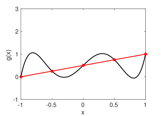
Figure 1: Example for which the algorithm based on hierarchical surplus fails. The function $g(x)=\frac{256}{30}x^{5}-\frac{32}{3}x^{3}+\frac{79}{30}x+\frac{1}{2}$ (in black) goes exactly through the red straight line at the points $x=-1,-0.5,0,0.5,1$. Calculating the piece-wise linear interpolant between two ($x=-1,1$), three ($x=-1,0,1$), and five ($x=-1,-\frac{1}{2},0,\frac{1}{2},1$) points would result in a null hierarchical surplus on these points.

A well known adaptive sampling algorithm is based on the calculation of the so-called hierarchical surplus [38, 28, 30, 39, see e.g]. This is defined as the difference, between two levels of refinement, in the solution obtained by the interpolant. Although this algorithm is quite robust, and it is especially efficient in detecting discontinuities, it has the obvious drawback that it can be prematurely terminated, whenever the interpolant happens to exactly pass through the true solution on a point where the hierarchical surplus is calculated, no matter how inaccurate the interpolant is in close-by regions (see Figure 1 for an example).

The goal of this paper is to describe an alternative strategy for the adaptive selection of sampling points. The objective in devising such strategy is to have a simple and robust set of rules for choosing the next sampling point. The paper is concerned with a proof-of-principle demonstration of our new strategy, and we will focus here on one dimensional cases and on the case of uniform $P_{X}$ only, postponing the generalization to multiple dimensions to future work. It is important to appreciate that the stated goal of this work is different from the traditional approach followed in the overwhelming majority of works that have presented sampling methods for UQ in the literature. Indeed, it is standard to focus on the convergence of the nonlinear unknown function $g(x)$, trying to minimize the interpolation error on $g(x)$, for a given number of sampling points. On the other hand, we will show that the convergence rates of $g(x)$ and of its cumulative distribution function can be quite different. Our new strategy is designed to achieve the fastest convergence on the latter quantity, which is ultimately the observable quantity of an experiment.

The paper is organized as follows. In Section 2 we define the mathematical methods used for the construction of the interpolant and show our adaptive strategy to choose a new collocation points. In Section 3 we present some numerical examples and comparisons with the Clenshaw-Curtis collocation method, and the adaptive method based on hierarchical surplus. Finally, we draw our conclusions in Section 4.

2 Mathematical methods

2.1 Clenshaw-Curtis (CC) quadrature rule

In Section 3, we compare our method with the CC method, which is the standard appropriate collocation method for a uniform $P_{X}$. Here, we recall the basic properties of CC, for completeness. The Clenshaw-Curtis (CC) quadrature rule uses the extrema of a Chebyshev polynomial (the so-called ‘extrema plus end-points’ collocation points in [40]) as abscissas. They are particularly appealing to be used as collocation points in UQ, because a certain subset of them are nested. Specifically, they are defined, in the interval $[-1,1]$ as:

$$x_{i}=-\cos\left(\frac{\pi(i-1)}{N-1}\right)\quad i=1,\dots,N.$$ (2)

One can notice that the the set of $N=2^{w}+1$ points is fully contained in the set of $N=2^{w+1}+1$ points (with $w$ an arbitrary integer, referred to as the level of the set). In practice this means that one can construct a nested sequence of collocation points with $N=3,5,9,17,33,65,129,\dots$, re-using all the previous evaluations of $g$.

Collocation points based on quadratures are optimal to calculate moments :

$$\mu_{Y}^{p}=\int y^{p}P_{Y}(y){\rm d}y=\int g(x)^{p}P_{X}(x){\rm d}x,$$ (3)

where we used the identity relation,

$$P_{Y}(y){\rm d}y=P_{X}(x){\rm d}x.$$ (4)

It is known that integration by quadrature is very accurate (for smooth enough integrand), and the moments can be readily evaluated, without the need to construct an interpolant:

$$\mu_{Y}^{p}\simeq\sum_{i}w_{i}(g(x_{i}))^{p},$$ (5)

where the weights $w_{i}$ can be computed with standard techniques (see, e.g. [36]). The interpolant for the CC method is the Lagrange polynomial.

2.2 Selection of collocation points based on hierarchical surplus

The hierarchical surplus algorithm is widely used for interpolation on sparse grids. It is generally defined as the difference between the value of an interpolant at the current and previous interpolation levels [38]:

$$\Delta^{n}=\tilde{g}^{n}-\tilde{g}^{n-1}$$ (6)

The simplest algorithm prescribes a certain tolerance and looks for all the point at the new level where the hierarchical surplus is larger than the tolerance. The new sampling points (at the next level, $n+1$) will be the neighbors (defined with a certain rule) of the points where this condition is met. In one-dimension, the algorithm is extremely simple because the neighbors are defined by only two points, that one can define in such a way that cells are always halved. In this work, we compare our new method with a slightly improved version of the hierarchical surplus algorithm. The reason is because we do not want our comparisons to be dependent on the choice of an arbitrary tolerance level, and we want to be able to add new points two at the time. Hence, we define a new interpolation level by adding only the two neighbors of the point with the largest hierarchical surplus. All the previous hierarchical surpluses that have been calculated, but for which new points have not been added yet are kept. The pseudo-code of the algorithm follows. The interpolant is understood to be piece-wise linear interpolation, and the grid is $x\in[-1,1]$.

Calculate the interpolant on the grid $x=\{-1,0,1\}$.

Define $x_{h}=\{-1/2,1/2\}$ and add them on the grid

while Not converged do

       Calculate the interpolant on the new grid

       Calculate the hierarchical surplus on the last two entries of $x_{h}$ and store them in the vector $h_{s}$

       Find the largest hierarchical surplus in $h_{s}$, remove it from $h_{s}$ and remove the corresponding $x$ from $x_{h}$

       Append the two neighbors to $x_{h}$ and add them to the grid

end while

Algorithm 1 Hierarchical surplus algorithm

2.3 Multiquadric biharmonic radial basis

We use a multiquadric biharmonic radial basis function (RBF) with respect to a set of points $\{x_{i}\}$, with $i=1,\dots,N$, defined as:

$$\Phi_{i}(x,c)=\sqrt{(x-x_{i})^{2}+c_{i}^{2}},$$ (7)

where $c_{i}$ are free parameters (referred to as shape parameters). The function $g(x)$ is approximated by the interpolant $\widetilde{g}(x)$ defined as

$$\widetilde{g}(x)=\sum_{i=1}^{N}\lambda_{i}\Phi_{i}(x,c).$$ (8)

The weights $\lambda_{i}$ are obtained by imposing that $g(x_{i})=\widetilde{g}(x_{i})$ for each sampling point in the set, namely the interpolation error is null at the sampling points. This results in solving a linear system for ${\bf\lambda}=(\lambda_{1},\dots,\lambda_{N})$ of the form $A{\bf\lambda}^{T}=g({\bf x})^{T}$, with $A$ a real symmetric $N\times N$ matrix. We note that, by construction, the linear system will become more and more ill-conditioned with increasing $N$, for fixed values of $c$. This can be easily understood because when two points become closer and closer the corresponding two rows in the matrix $A$ become less and less linearly independent. To overcome this problem one needs to decrease the corresponding values of $c$. In turns, this means that the interpolant $\widetilde{g}(x)$ will tend to a piece-wise linear interpolant for increasingly large $N$.

2.4 New adaptive selection of collocation points

We focus, as the main diagnostic of our method, on the cumulative distribution function (cdf) $C(y)$, which is defined as

$$C(y)=\int_{y_{\rm min}}^{y}P_{Y}(y){\rm d}y,$$ (9)

where $y_{\rm min}=\min g(x)$. As it is well known, the interpretation of the cumulative distribution function is that, for a given value $y^{*}$, $C(y^{*})$ is the probability that $g(x)\leq y^{*}$. Of course, the cdf $C(y)$ contains all the statistical information needed to calculate any moment of the distribution, and can return the probability density function $P_{Y}(y)$, upon differentiation. Moreover, the cdf is always well defined between 0 and 1. The following two straightforward considerations will guide the design of our adaptive selection strategy. A first crucial point, already evident from Eq. (1), is whether or not $g(x)$ is bijective. When $g(x)$ is bijective this translates to the cdf $C(y)$ being continuous, while a non-bijective function $g(x)$ produces a cdf $C(y)$ which is discontinuous. It follows that intervals in $x$ where $g(x)$ is constant (or nearly constant) will map into a single value $y=g(x)$ (or a very small interval in $y$) where the cdf will be discontinuous (or ‘nearly’ discontinuous). Secondly, an interval in $x$ with a large first derivative of $g(x)$ will produce a nearly flat cdf $C(y)$. This is again clear by noticing that the Jacobian $J$ in Eq. (1) (${\rm d}g(x)/{\rm d}x$ in one dimension) is in the denominator, and therefore the corresponding $P_{Y}(y)$ will be very small, resulting in a flat cdf $C(y)$.
Loosely speaking one can then state that regions where $g(x)$ is flat will produce large jumps in the cdf $C(y)$ and, conversely, regions where the $g(x)$ has large jumps will map in to a nearly flat cdf $C(y)$. From this simple considerations one can appreciate how important it is to have an interpolant that accurately capture both regions with very large and very small first derivative of $g(x)$. Moreover, since the cdf $C(y)$ is an integrated quantity, interpolation errors committed around a given $y$ will propagate in the cdf for all larger $y$ values. For this reason, it is important to achieve a global convergence with interpolation errors that are of the same order of magnitude along the whole domain.
The adaptive section algorithm works as follows. We work in the interval $x\in[-1,1]$ (every other interval where the support of $g(x)$ is defined can be rescaled to this interval). We denote with $\{x_{i}\}$ the sampling set which we assume is always sorted, such that $x_{i}<x_{i+1}$. We start with 3 points: $x_{1}=-1$, $x_{2}=0$, $x_{3}=1$. For the robustness and the simplicity of the implementation we choose to select a new sampling point always at equal distance between two existing points. One can decide to limit the ratio between the largest and smallest distance between adjacent points: $r=\max\{d_{i}\}/\min\{d_{i}\}$ (with $i=1,\dots,N-1$), where $d_{i}$ is the distance between the points $x_{i+1}$ and $x_{i}$. This avoids to keep refining small intervals when large intervals might still be under-resolved, thus aiming for the above mentioned global convergence over the whole support. At each iteration we create a list of possible new points, by halving every interval, excluding the points that would increase the value of $r$ above the maximum desired (note that $r$ will always be a power of 2). We calculate the first derivative of $\widetilde{g}(x)$ at these points, and alternatively choose the point with largest/smallest derivative as the next sampling point. Notice that, by the definition of the interpolant, Eq. (8), its first derivative can be calculated exactly as:

$$\frac{{\rm d}\widetilde{g}(x)}{{\rm d}x}=\sum_{i=1}^{N}\lambda_{i}\frac{{\rm d}\Phi_{i}(x,c)}{{\rm d}x}$$ (10)

without having to recompute the weights $\lambda_{i}$. At each iteration the shape parameters $c_{i}$ are defined at each points, as $c_{i}=0.85\cdot\min(d_{i-1},d_{i})$, i.e. they are linearly rescaled with the smallest distance between the point $x_{i}$ and its neighbors. The pseudo-code of the algorithm follows.

while Not converged do

       $x_{\rm guess}\leftarrow 0.5\cdot(x_{i}+x_{i+1})$

       Exclude points in $x_{\rm guess}$ such that $r=\max\{d_{i}\}/\min\{d_{i}\}>R$

       Calculate $\widetilde{g}^{n}(x)^{\prime}$ through (10) at $\{x_{\rm guess}\}$

       Alternatively choose $x_{\rm guess}$ with largest/smallest values of $|\widetilde{g}^{n}(x)^{\prime}|$ as new collocation point

       Calculate new weights $\lambda_{i}$

end while

Algorithm 2 Adaptive selection of sampling points

3 Numerical examples

In this section we present and discuss four numerical examples where we apply our adaptive selection strategy. In this work we focus on a single input parameter and the case of constant probability $P_{X}=1/2$ in the interval $x\in[-1,1]$, and we compare our results against the Clenshaw-Curtis, and the hierarchical surplus methods. We denote with $\widetilde{g}^{n}(x)$ the interpolant obtained with a set of $n$ points (hence the iterative procedure starts with $\widetilde{g}^{3}(x)$). A possible way to construct the cdf $C(y)$ from a given interpolant $\widetilde{g}^{n}(x)$ would be to generate a sample of points in the domain $[-1,1]$, randomly distributed according to the pdf $P_{X}(x)$, collecting the corresponding values calculated through Eq. (8), and constructing their cdf. Because here we work with a constant $P_{X}(x)$, it is more efficient to simply define a uniform grid in the domain $[-1,1]$ where to compute $\widetilde{g}^{n}(x)$. In the following we will use, in the evaluation of the cdf $C(y)$, a grid in $y$ with $N_{y}=10001$ points equally spaced in the interval $[\min\widetilde{g}^{n}(x),\max\widetilde{g}^{n}(x)]$, and a grid in $x$ with $N_{x}=1001$ points equally spaced in the interval $[-1,1]$. We define the following errors:

$$\varepsilon_{C}=\frac{||C(\widetilde{g}^{n}(x))-C(g(x))||_{2}}{\sqrt{N_{y}}}$$ (11)

$$\varepsilon_{g}=\frac{||\widetilde{g}^{n}(x)-g(x)||_{2}}{\sqrt{N_{x}}}$$ (12)

where $||\cdot||_{2}$ denotes the L₂ norm. It is important to realize that the accuracy of the numerically evaluated cdf $C(y)$ will always depend on the binning of $y$, i.e. the points at which the cdf is evaluated. As we will see in the following examples, the error $\varepsilon_{C}$ saturates for large $N$, which thus is an artifact of the finite bin size. We emphasize that, differently from most of the previous literature, our strategy focuses on converging rapidly in $\varepsilon_{C}$, rather than in $\varepsilon_{g}$. Of course, a more accurate interpolant will always result in a more accurate cdf, however the relationship between a reduction in $\varepsilon_{g}$ and a corresponding reduction in $\varepsilon_{C}$ is not at all trivial. This is because the relation between $P_{X}(x)$ and $P_{Y}(y)$ is mediated by the Jacobian of $g(x)$, and it also involves the bijectivity of $g$.
Finally, we study the convergence of the mean $\mu_{Y}$, see equation 3, and the variance $\sigma_{Y}^{2}$, which is defined as

$$\sigma_{Y}^{2}=\int_{-1}^{1}(\widetilde{g}(x)-\mu_{Y})^{2}P_{X}(x)\textrm{d}x.$$ (13)

These will be calculated by quadrature for the CC methods, and with an integration via trapezoidal method for the adaptive methods.
We study two analytical test cases:

• Case 1: $g(x)=\arctan(10^{3}x^{3})$;

• Case 2: $g(x)=\frac{1}{(2+\sin(3\pi x))^{2}}$;

and two test cases where an analytical solution is not available, and the reference $g(x)$ will be calculated as an accurate numerical solution of a set of ordinary differential equations:

• Case 3: Lotka-Volterra model (predator-prey);

• Case 4: Van der Pol oscillator.

While Case 1 and 2 are more favorable to the CC method, because the functions are smooth and analytical, hence a polynomial interpolation is expected to produce accurate results, the latter two cases mimic applications of real interest, where the model does not produce analytical results, although $g(x)$ might still be smooth (at least piece-wise, in Case 4).

3.1 Case 1: $g(x)=\arctan(10^{3}x^{3})$

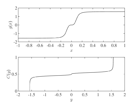
Figure 2: Case 1: $g(x)=\arctan(10^{3}x^{3})$. Top panel: $g(x)$; bottom panel: cdf $C(y)$.

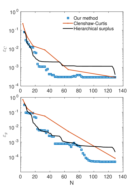
Figure 3: Case 1. Error $\varepsilon_{C}$ (top) $\varepsilon_{g}$ (bottom) as function of number of sampling points $N$. Blue squares: new adaptive selection method. Red dots: Clenshaw-Curtis. Black curve: adaptive method based on hierarchical surplus.

In this case $g(x)$ is a bijective function, with one point ($x=0$) where the first derivative vanishes. Figure 2 shows the function $g(x)$ (top panel) and the corresponding cdf $C(y)$ (bottom panel), which in this case can be derived analytically. Hence, we use the analytical expression of cdf $C(y)$ to evaluate the error $\varepsilon_{C}$. The convergence of $\varepsilon_{C}$ and $\varepsilon_{g}$ is shown in Figure 3 (top and bottom panels, respectively). Here and in all the following figures blue squares denote the new adaptive selection method, red dots are for the CC methods, and black line is for the hierarchical surplus method. We have run the CC method only for $N=3,5,9,17,33,65,129$ (i.e. the points at which the collocation points are nested), but for a better graphical visualization the red dots are connected with straight lines. One can notice that the error for the new adaptive method is consistently smaller than for the CC method. From the top panel, one can appreciate the saving in computer power that can be achieved with our new method. Although the difference with CC is not very large until $N=17$, at $N=33$ there is an order of magnitude difference between the two. It effectively means that in order to achieve the same error $\varepsilon_{C}\sim 10^{-5}$, the CC method would run at least twice the number of simulations. The importance of focusing on the convergence of the cdf, rather than on the interpolant, is clear in comparing our method with the hierarchical surplus method. For instance, for $N=80$, the two methods have a comparable error $\varepsilon_{g}$, but our method has achieved almost an order of magnitude more accurate solution in $C(y)$. Effectively, this means that our method has sampled the new points less redundantly. In this case $g(x)$ is an anti-symmetric function with zero mean. Hence, any method that chooses sampling points symmetrically distributed around zero would produce the correct first moment $\mu_{Y}$. We show in figure 4 the convergence of $\sigma_{Y}^{2}$, as the absolute value of the different with the exact value $\sigma_{an}$, in logarithmic scale. Blue, red, and black lines represent the new adaptive method, the CC, and the hierarchical surplus methods, respectively (where again for the CC, simulations are only performed where the red dots are shown). The exact value is $\sigma_{an}^{2}=2.102$. As we mentioned, the CC method is optimal to calculate moments, since it uses quadrature. Although in our method the error does not decrease monotonically, it is comparable with the result for CC.

3.2 Case 2: $g(x)=\frac{1}{(2+\sin(3\pi x))^{2}}$

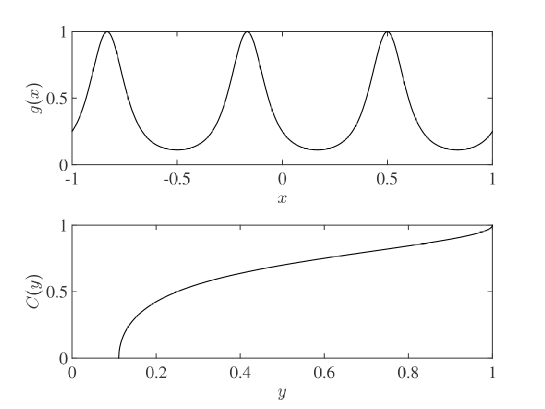
Figure 5: Case 2: $g(x)=\frac{1}{(2+\sin(3\pi x))^{2}}$. Top panel: $g(x)$; bottom panel: $C(y)$.

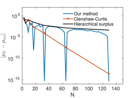
Figure 7: Case 2. Absolute error in the mean $\mu_{Y}$ versus number of sampling points $N$. Blue: new adaptive selection method. Red: Clenshaw-Curtis. Black: adaptive method based on hierarchical surplus.

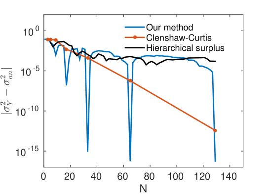
Figure 8: Case 2. Absolute error in the variance $\sigma_{Y}^{2}$ versus number of sampling points $N$. Blue: new adaptive selection method. Red: Clenshaw-Curtis. Black: adaptive method based on hierarchical surplus.

In this case the function $g(x)$ is periodic, and it presents, in the domain $x\in[-1,1]$ three local minima ($y=1/9$) and three local maxima ($y=1$). The function and the cdf $C(y)$ are shown in Figure 5 (top and bottom panel, respectively). Figure 6 shows the error for this case (from now on the same format of Figure 3 will be used). The first consideration is that the hierarchical surplus method is the less accurate of the three. Second, $\varepsilon_{g}$ is essentially the same for the CC and the new method, up to $N=65$. For $N=129$ the CC methods achieve a much accurate solution as compared to the new adaptive method, whose error has a much slower convergence. However, looking at the error in the cdf in top panel of Figure 6, the two methods are essentially equivalent. This example demonstrates that, in an UQ framework, the primary goal in constructing a good interpolant should not be to minimize the error of the interpolant with respect to the ’true’ $g(x)$, but rather to achieve the fastest possible convergence on the cdf $C_{Y}$. Although, the two effects are intuitively correlated, they are not into a linear relationship. In other words, not all sample points in $x$ count equally in minimizing $\varepsilon_{C}$. The convergence of $\mu_{Y}$ (exact value $\mu_{an}=0.385$) and $\sigma_{Y}^{2}$ (exact value $\sigma_{an}=0.087$) is shown in Figures 7 and 8, respectively. It is interesting to notice that our method presents errors that are always smaller than the CC method, although the errors degrade considerably in the regions between two CC points, where the two adaptive methods yield comparable results.

3.3 Case 3: Lotka-Volterra model (predator-prey)

The Lotka-Volterra model [41, 42, 43] is a well-studied model that exemplifies the interaction between two populations (predators and preys). This case is more realistic than Cases 1 and 2, as the solution of the model cannot be written in analytical form. As such, both the $g(x)$ and the cdf $C(y)$ used to compute the errors are calculated numerically. We use the following simple model:

$$\frac{{\rm d}h(t)}{{\rm d}t} = h(t)-(5x+6)h(t)l(t)$$ (14)

$$\frac{{\rm d}l(t)}{{\rm d}t} = h(t)l(t)-l(t)$$ (15)

where $h(t)$ and $l(t)$ denote the population size for each species (say, horses and lions) as function of time. The ODE is easily solved in MATLAB, with the ode45 routine, with an absolute tolerance set equal to $10^{-8}$. We use, as initial conditions, $h(t=0)=l(t=0)=1$, and we solve the equations for $t\in[0,10]$. Clearly, the solution of the model depends on the input parameter $x$. We define our test function $g(x)$ to be the result of the model for the $l$ population at time $t=10$:

$$g(x)=l(t=10,x).$$ (16)

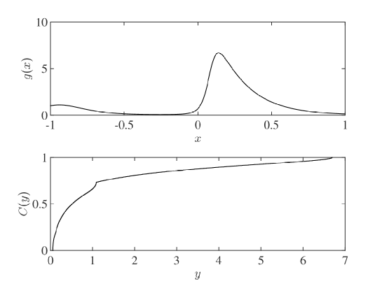
Figure 9: Case 3: Lotka-Volterra model. Top panel: $g(x)$; bottom panel: $C(y)$.

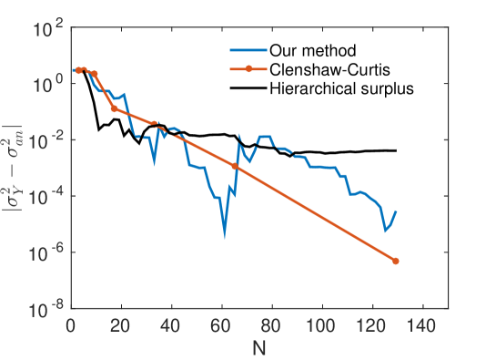
Figure 12: Case 3. Absolute error in the variance $\sigma_{Y}^{2}$ versus number of sampling points $N$. Blue: new adaptive selection method. Red: Clenshaw-Curtis. Black: adaptive method based on hierarchical surplus.

The resulting function $g(x)$, and the computed cdf $C(y)$ are shown in Figure 9 (top and bottom panel, respectively). We note that, although $g(x)$ cannot be expressed as an analytical function, it is still smooth, and hence it does not present particular difficulties in being approximated through a polynomial interpolant. Indeed the error $\varepsilon_{g}$ undergoes a fast convergence both for the adaptive methods and for the CC method (Figure 10). Once again, the new adaptive method is much more powerful than the CC method in achieving a better convergence rate, and thus saving computational power, while the hierarchical surplus method is the worst of the three. Convergence of $\mu_{Y}$ and $\sigma_{Y}^{2}$ are shown in Figures 11 and 12, respectively. Similar to previous cases, the CC presents a monotonic convergence, while this is not the case for the adaptive methods. Only for $N=129$, the CC method yields much better results than the new method.

3.4 Case 4: Van der Pol oscillator

Our last example is the celebrated Van der Pol oscillator[44, 7, 45, 46], which has been extensively studied as a textbook case of a nonlinear dynamical system. In this respect this test case is very relevant to Uncertainty Quantification, since real systems often exhibit a high degree of nonlinearity. Similar to Case 3, we define our test function $g(x)$ as the output of a set of two ODEs, which we solve numerically with MATLAB. The model for the Van der Pol oscillator is:

$$\frac{{\rm d}Q(t)}{{\rm d}t} = V(t)$$ (17)

$$\frac{{\rm d}V(t)}{{\rm d}t} = (-50+100(x+2))(1-Q(t)^{2})V(t)-Q(t).$$ (18)

The initial conditions are $Q(t=0)=2$, $V(t=0)=0$. The model is solved for time $t\in[0,300]$, and the function $g(x)$ is defined as

$$g(x)=V(t=300,x).$$ (19)

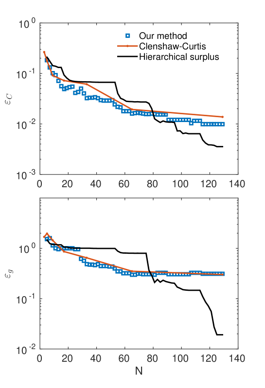
Figure 14: Case 4. Error $\varepsilon_{C}$ (top) $\varepsilon_{g}$ (bottom) as function of number of sampling points $N$. Blue squares: new adaptive selection method. Red dots: Clenshaw-Curtis. Black curve: adaptive method based on hierarchical surplus.

The so-called nonlinear damping parameter is rescaled such that for $x\in[-1,1]$, it ranges between 50 and 250. The function $g(x)$ and the corresponding cdf $C(y)$ are shown in Figure 13. This function is clearly much more challenging than the previous ones. It is divided in two branches, where it takes values $-2\leq y\leq-1$ and $1\leq y\leq 2$, and it presents discontinuities where it jumps from one branch to the other. Correspondingly, cdf $C(y)$ presents a flat plateau for $-1\leq y\leq 1$, which is the major challenge for both methods. In figure 14 we show the errors $\varepsilon_{g}$ and $\varepsilon_{C}$. The overall convergence rate of the CC and the new method is similar. For this case, the hierarchical surplus method yields a better convergence, but only for $N>80$. As we commented before, the mean $\mu_{Y}$ has no statistical meaning in this case, because the output is divided into two separate regions. The convergence for $\sigma_{Y}^{2}$ is presented in Figure 15.

4 Conclusions and future work

We have presented a new adaptive algorithm for the selection of sampling points for non-intrusive stochastic collocation in Uncertainty Quantification (UQ). The main idea is to use a radial basis function as interpolant, and to refine the grid on points where the interpolant presents large and small first derivative.
In this work we have focused on 1D and uniform probability $P_{X}(x)$, and we have shown four test cases, encompassing analytical and non-analytical smooth functions, which are prototype of a very wide class of functions. In all cases the new adaptive method improved the efficiency of both the (non-adaptive) Clenshaw-Curtis collocation method, and of the adaptive algorithm based on the calculation of the hierarchical surplus (note that the method used in this paper is a slight improvement of the classical algorithm). The strength of our method is the ability to select a new sampling point making full use of the interpolant resulting from all the previous evaluation of the function $g(x)$, thus seeking the most optimal convergence rate for the cdf $C(y)$. We have shown that there is no one-to-one correspondence between a reduction in the interpolation error $\varepsilon_{g}$ and a reduction in the cdf error $\varepsilon_{C}$. For this reason, collocation methods that choose the distribution of sampling points a priori can perform poorly in attaining a fast convergence rate in $\varepsilon_{C}$, which is the main goal of UQ. Moreover, in order to maintain the nestedness of the collocation points the CC method requires larger and larger number of simulations ($2^{w}$ moving from level $w$ to level $w+1$), which is in contrast with our new method where one can add one point at the time.
We envision many possible research directions to further investigate our method. The most obvious is to study multi-dimensional problems. We emphasize that the radial basis function is a mesh-free method and as such we anticipate that this will largely alleviate the curse of dimensionality that afflicts other collocation methods based on quadrature points (however, see [29] for methods related to the construction of sparse grids, which have the same aim). Moreover, it will be interesting to explore the versatility of RBF in what concerns the possibility of choosing an optimal shape parameter $c$ [47]. Recent work [48, 49] investigated the role of the shape parameter $c$ in interpolating discontinuous functions, which might be very relevant in the context of UQ, when the continuity of $g(x)$ cannot be assumed a priori. Finally, a very appealing research direction, would be to simultaneously exploit quasi-Monte Carlo and adaptive selection methods for extremely large dimension problems.

Figure 4: Case 1. Absolute error in the variance $\sigma_{Y}^{2}$ versus number of sampling points $N$. Blue: new adaptive selection method. Red: Clenshaw-Curtis. Black: adaptive method based on hierarchical surplus.

Figure 6: Case 2. Error $\varepsilon_{C}$ (top) $\varepsilon_{g}$ (bottom) as function of number of sampling points $N$. Blue squares: new adaptive selection method. Red dots: Clenshaw-Curtis. Black curve: adaptive method based on hierarchical surplus.

Figure 10: Case 3. Error $\varepsilon_{C}$ (top) $\varepsilon_{g}$ (bottom) as function of number of sampling points $N$. Blue squares: new adaptive selection method. Red dots: Clenshaw-Curtis. Black curve: adaptive method based on hierarchical surplus.

Figure 11: Case 3. Absolute error in the mean $\mu_{Y}$ versus number of sampling points $N$. Blue: new adaptive selection method. Red: Clenshaw-Curtis. Black: adaptive method based on hierarchical surplus.

Figure 13: Case 4: Van der Pol oscillator. Top panel: $g(x)$; bottom panel: $C(y)$.

Figure 15: Case 4. Absolute error in the variance $\sigma_{Y}^{2}$ versus number of sampling points $N$. Blue: new adaptive selection method. Red: Clenshaw-Curtis. Black: adaptive method based on hierarchical surplus.

- [1] Xiu, D., Fast numerical methods for stochastic computations: a review, Communications in computational physics, 5(2-4):242–272, 2009.
- [2] Eldred, M. and Burkardt, J., Comparison of non-intrusive polynomial chaos and stochastic collocation methods for uncertainty quantification, AIAA paper, 976(2009):1–20, 2009.
- [3] Onorato, G., Loeven, G., Ghorbaniasl, G., Bijl, H., and Lacor, C., Comparison of intrusive and non-intrusive polynomial chaos methods for cfd applications in aeronautics, In V European Conference on Computational Fluid Dynamics ECCOMAS, Lisbon, Portugal, pp. 14–17, 2010.
- [4] Xiu, D. and Karniadakis, G.E., The wiener–askey polynomial chaos for stochastic differential equations, SIAM journal on scientific computing, 24(2):619–644, 2002.
- [5] Crestaux, T., Le Maıˆtre, O., and Martinez, J.M., Polynomial chaos expansion for sensitivity analysis, Reliability Engineering & System Safety, 94(7):1161–1172, 2009.
- [6] Togawa, K., Benigni, A., and Monti, A., Advantages and challenges of non-intrusive polynomial chaos theory, In Proceedings of the 2011 Grand Challenges on Modeling and Simulation Conference, GCMS ’11, pp. 30–35, Vista, CA, 2011. Society for Modeling & Simulation International.
- [7] Eldred, M.S., Recent advances in non-intrusive polynomial chaos and stochastic collocation methods for uncertainty analysis and design, AIAA Paper, 2274:2009, 2009.
- [8] Tempone, I.B.I.R. and G.Zouraris, Galerkin finite element approximations of stochastic elliptic partial differential equations, SIAM Journal of Numerical Analysis, 42(2):800–825, 2004.
- [9] Grigoriu, M., Stochastic systems: uncertainty quantification and propagation, Springer Science & Business Media, 2012.
- [10] Xiu, D., Numerical methods for stochastic computations: a spectral method approach, Princeton University Press, 2010.
- [11] Le Maître, O. and Knio, O.M., Spectral methods for uncertainty quantification: with applications to computational fluid dynamics, Springer Science & Business Media, 2010.
- [12] Caflisch, R.E., Monte carlo and quasi-monte carlo methods, Acta Numerica, 7:1–49, 1998.
- [13] Kalos, M.H. and Whitlock, P.A., Monte carlo methods, John Wiley & Sons, 2008.
- [14] L’Ecuyer, P. and Owen, A.B., Monte Carlo and Quasi-Monte Carlo Methods 2008, Springer, 2009.
- [15] Niederreiter, H.G., Quasi-monte carlo methods and pseudo-random numbers, Bull. Amer. Math. Soc., 84(6):957–1041, 1978.
- [16] Kalos, M.H. and Whitlock, P.A., Pseudorandom numbers, Monte Carlo Methods, Second Edition, pp. 179–197, 2008.
- [17] Bellman, R., Dynamic programming, Courier Dover Publications, 2003.
- [18] Indyk, P. and Motwani, R., Approximate nearest neighbors: towards removing the curse of dimensionality, In Proceedings of the thirtieth annual ACM symposium on Theory of computing, pp. 604–613. ACM, 1998.
- [19] Kuo, F.Y. and Sloan, I.H., Lifting the curse of dimensionality, Notices of the AMS, 52(11):1320–1328, 2005.
- [20] Xiu, D. and Hesthaven, J.S., High-order collocation methods for differential equations with random inputs, SIAM J. Sci. Comput., 28:1167–1185, 2006.
- [21] Foo, J. and Karniadakis, G.E., Multi-element probabilistic collocation method in high dimensions, J. Comput. Phys., 229(5):1536–1557, March 2010.
- [22] Babuška, I., Nobile, F., and Tempone, R., A stochastic collocation method for elliptic partial differential equations with random input data, SIAM Journal on Numerical Analysis, 45(3):1005–1034, 2007.
- [23] Wang, P. and Tartakovsky, D.M., Uncertainty quantification in kinematic-wave models, Journal of computational Physics, 231(23):7868–7880, 2012.
- [24] Wang, P., Tartakovsky, D.M., Jarman Jr, K., and Tartakovsky, A.M., Cdf solutions of buckley–leverett equation with uncertain parameters, Multiscale Modeling & Simulation, 11(1):118–133, 2013.
- [25] Smolyak, S.A., Quadrature and interpolation formulas for tensor products of certain classes of functions, In Dokl. Akad. Nauk SSSR, Vol. 4, p. 123, 1963.
- [26] Ganapathysubramanian, B. and Zabaras, N., Sparse grid collocation schemes for stochastic natural convection problems, Journal of Computational Physics, 225(1):652–685, 2007.
- [27] Bieri, M., Andreev, R., and Schwab, C., Sparse tensor discretization of elliptic spdes, SIAM Journal on Scientific Computing, 31(6):4281–4304, 2009.
- [28] Ma, X. and Zabaras, N., An efficient bayesian inference approach to inverse problems based on an adaptive sparse grid collocation method, Inverse Problems, 25(3):035013, 2009.
- [29] Tempone, F.N.R. and Webster, C.G., A sparse grid stochastic collocation method for partial differential equations with random input data, SIAM J. Numer. Anal., 46(5):2309–2345, 2008.
- [30] Jakeman, J.D. and Roberts, S.G. Local and dimension adaptive stochastic collocation for uncertainty quantification. In Sparse grids and applications, pp. 181–203. Springer, 2012.
- [31] Nguyen, N.H., Willcox, K., and Khoo, B.C., Model order reduction for stochastic optimal control, In ASME 2012 11th Biennial Conference on Engineering Systems Design and Analysis, pp. 599–606. American Society of Mechanical Engineers, 2012.
- [32] Laurie, P.D., Computation of gauss-type quadrature formulas, J. Comp. Appl. Math., 127(1-2):201–217, 2001.
- [33] Gautschi, W., On the construction of gaussian quadrature rules from modified moments., Mathematics of Computation, 24(110):245–260, 1970.
- [34] Waldvogel, J., Fast construction of the fejér and clenshaw–curtis quadrature rules, BIT Numerical Mathematics, 46(1):195–202, 2006.
- [35] Berrut, J.P. and Trefethen, L.N., Barycentric lagrange interpolation, SIAM Rev., 46(3):501–517, 2004.
- [36] Trefethen, L.N., Spectral methods in matlab, SIAM: Society for Industrial and Applied Mathematics, 2000.
- [37] Epperson, J., On the runge example, Amer. Math. Monthly, 94:329–341, 1987.
- [38] Ma, X. and Zabaras, N., An adaptive hierarchical sparse grid collocation algorithm for the solution of stochastic differential equations, Journal of Computational Physics, 228(8):3084–3113, 2009.
- [39] Witteveen, J.A. and Iaccarino, G., Refinement criteria for simplex stochastic collocation with local extremum diminishing robustness, SIAM Journal on Scientific Computing, 34(3):A1522–A1543, 2012.
- [40] Boyd, J.P., Chebychev and fourier spectral methods, 2nd ed., Dover, New York, 2001.
- [41] Baruer, F. and Castillo-Chavez, C., Mathematical models in population biology and epidemiology, Springer-Verlag, 2000.
- [42] Stevens, M.H.H. Lotka–volterra interspecific competition. In A Primer of Ecology with R, pp. 135–159. Springer, 2009.
- [43] Wangersky, P.J., Lotka-volterra population models, Annual Review of Ecology and Systematics, pp. 189–218, 1978.
- [44] Geer, M.B.D.J. and Andersen, C.M., Perturbation analysis of the limit cycle of the free van der pol equation, SIAM Journal on Applied Mathematics, 44(5):881–895, 1984.
- [45] Yuan, R., Wang, X., Ma, Y., Yuan, B., and Ao, P., Exploring a noisy van der pol type oscillator with a stochastic approach, Phys. Rev. E, 87:062109, Jun 2013.
- [46] Liu, L., Dowell, E.H., and Hall, K.C., A novel harmonic balance analysis for the van der pol oscillator, International Journal of Non-Linear Mechanics, 42(1):2–12, 2007.
- [47] Fasshauer, G.E. and Zhang, J.G., On choosing “optimal” shape parameters for rbf approximation, Numer. Algor., 45:345–368, 2007.
- [48] Jung, J.H. and Durante, V.R., An iterative adaptive multiquadric radial basis function method for the detection of local jump discontinuities, Applied Numerical Mathematics, 59(7):1449–1466, 2009.
- [49] Wang, J. and Liu, G., On the optimal shape parameters of radial basis functions used for 2-d meshless methods, Computer methods in applied mechanics and engineering, 191(23):2611–2630, 2002.