How fast does the clock of Finance run? – A time-definition enforcing scale invariance and quantifying overnights

Abstract

A symmetry-guided definition of time may enhance and simplify the analysis of historical series with recurrent patterns and seasonalities. By enforcing simple-scaling and stationarity of the distributions of returns, we identify a successful protocol of time definition in Finance. The essential structure of the stochastic process underlying the series can thus be analyzed within a most parsimonious symmetry scheme in which multiscaling is reduced in the quest of a time scale additive and independent of moment-order in the distribution of returns. At the same time, duration of periods in which markets remain inactive are properly quantified by the novel clock, and the corresponding (e.g., overnight) returns are consistently taken into account for financial applications.

I Introduction

Relativity theory Wald (1984) provides a remarkable example of the construction of a nontrivial time scale on the basis of a symmetry principle; namely, the proper time of a moving body from the requirement of invariance of the laws of Nature for different observers. This example, in which symmetry lays at the very foundation of the physical theory, may suggest to look for other contexts in which symmetries could help in defining useful notions of time. Nonstationary time series are very frequently encountered in fields like Meteorology Ivanova et al. (1999), Seismology Corral (2004, 2006), Physiology Peng et al. (1995, 2001); Hausdorff et al. (1995), Economy and Finance Liu et al. (1997); Galluccio et al. (1997); Bassler et al. (2007). The nonstationary mark limits the applicability of statistical methods in the quest for the process characterizing the series Tsay (2002), and may convey spurious effects in the detection of correlations in the time series Peng et al. (1994); Kantelhardt et al. (2002). Depending on the quality of the stochastic process, different strategies can be applied to simplify the signals and to recover stationarity properties. For instance, various detrending procedures have been proposed Peng et al. (1994); Kantelhardt et al. (2002), although in the general case their success is not always guaranteed Chen et al. (2002); Bryce et al. (2012). Other approaches Dacorogna et al. (1996, 2001); Zumbach (2002); Corral (2004) are instead based on a reassessment of the time stamp in terms of which the series is recorded. In particular, in the case of seismology it has been recently advanced Corral (2004, 2006) that the distribution of interoccurrence times between earthquakes becomes scale-invariant under a proper redefinition of time; the latter renders interoccurrencies stationary on the basis of the Omori’s aftershock law Omori (1984).

Following inspiration provided by the example of relativity, within the context of time series affected by cyclic nonstationary behavior Gardner et al. (2006) we show here that one can promote the approximate fulfillment of a simple scaling symmetry to become an operative criterion for the definition of a novel time, which we call financial scaling time (FST). Our focus is on Finance, a field in which the very definition of time constitutes a long-standing problem, while the application of symmetry principles lacks a strong tradition. As one should expect, the symmetry enforcement leads to a distinct simplification of the analysis. Specifically we show that financial returns, which are nonstationary in physical time, become so in FST. Within the financial context, multiscaling has been largely reported as a “stylized fact” and has inspired the construction of multifractal models Frisch (1997); Mandelbrot (1998); Calvet and Fischer (2002); Borland et al. (2005); Di Matteo (2007); Bacry (2008). Although we prove in Appendix A that our time redefinition cannot completely remove multiscaling effects, we concurrently show that they are in fact reduced in FST; consistently, the probability density functions (PDF) of returns satisfy simple scaling to a good approximation in a rather wide range of time scales. The FST also offers a natural quantification of the time elapsing during markets closures, so that the associated returns can be consistently taken into account in financial applications. Albeit focused on Finance, our methodology could be of broader physical interest – for instance in the analysis of interoccurrence times Corral (2004, 2006); Bogachev et al. (2007) – exemplifying how a symmetry-based time transformation may render a stochastic process stationary, as required in many statistical approaches Chicheportiche et al. (2014, 2017).

A clock properly adjusted to financial activity is not easy to identify. Financial markets have to cope with human daily routines throughout the world and bursts and doldrums occur at various time scales. In addition, during nights, weekends, and festivities, transactions stop in most cases. These interruptions, at the end of which assets prices turn out to have changed anyhow, together with the recurrent patterns in the activity (seasonalities), immediately signal the inadequacy of “natural” physical time as the appropriate one in terms of which to describe the stochastic evolution of financial markets. Besides physical time, different alternatives have been studied Clark (1973); Dacorogna et al. (2001); Ané et al. (1999); Stanley (2000); Jensen et al. (2004); Gillemot et al. (2006), including trading time, volume time, and tick-by-tick time. A time definition (theta-time) has also been put forward with the specific intent of getting rid of the seasonalities in financial time series Dacorogna et al. (1996, 2001); Zumbach (2002). Theta-time is designed to record the progress of market activity through the increase of the volatility as measured by the average absolute return. For the latter a power-law behavior is assumed as a function of physical time, but no discussion of the univocity of this time definition and of its effectiveness in enforcing stationarity of the return PDF is made. In most theoretical studies, inactive market periods are cut from the analyzed dataset and the corresponding returns ignored Dacorogna et al. (2001). However, the practice of ignoring inactive periods destroys the correspondence between the sum of returns and the real asset price, and as such it is thus not suitable to many financial applications. Alternatively, one could assign an arbitrary time interval to overnight and similar returns, but this implies altering the time scaling properties of their PDFs. Hence, the appropriate duration to be ascribed to overnight and similar returns remains an open issue. In general, there is also little focus on the requirement that increments over intervals of equal span should be identically distributed in order to make statistical sampling (e.g., sliding-window) applicable.

Here we show that a solution to these problems is naturally suggested by the existence of an approximate symmetry which appears when the PDFs increments over different intervals are compared. Indeed, from days to several weeks, the empirical financial returns’ PDFs are found to be approximately scale-invariant, in a sense familiar from the Physics of critical phenomena Baldovin and Stella (2007). Defining financial returns $r$ over the time span $\Delta t$ (here $\Delta t$ is an integer number of days) as the log-difference of the asset price value $s$, $r\equiv\ln s(t)-\ln s(t-\Delta t)$, this means that the empirical PDFs of $r$ over different $\Delta t$’s can be approximately collapsed onto each other in force of the scaling law

$$p(r,\Delta t)\simeq\frac{1}{\Delta t^{H}}\;g\left(\frac{r}{\Delta t^{H}}\right),$$ (1)

where $H$ is called the Hurst exponent Hurst (1951), and $g$, which is not Gaussian, is a scaling function. It turns out that $H$ is close to $1/2$ for assets of developed markets Galluccio et al. (1997); Di Matteo et al. (2005).

As discussed in Appendix A, a natural way of defining time is that of referring to a specific $q$-th order moment of the return PDF’s, $\mathbb{E}[|r|^{q}]$ $(q>0)$, assuming that the time interval is directly measured by this moment. This definition promotes the stationarity of the PDF over intervals of equal duration in the new time scale. However, we shown in Appendix A that only if in the novel time the PDF satisfies a form of simple scaling like in Eq. (1) with $H=1/2$, the time definition is independent of the chosen moment order and the novel time is additive. On the contrary, a simple scaling with $H\neq 1/2$ would prevent additivity and, most important, in the case of multiscaling, when $H$ depends on the moment order $q$, the time scales are different for different orders and there is no more a unique additive time in terms of which one can describe the returns aggregation process.

The strict validity of Eq. (1) with $H=1/2$ in physical time would thus establish an univoque correspondence between returns’ PDFs and time intervals durations $\Delta t$’s and we could say that physical time provides the time scale we are in quest of. However, Eq. (1) definitely does not hold at the intraday time scales, where nonstationarities affect the PDFs for returns defined over intervals with equal physical time duration Galluccio et al. (1997); Bassler et al. (2007); Allez et al. (2011), and $H$ can be very different from $1/2$ in selected time windows Bassler et al. (2007); Baldovin et al. (2015). Even in the interday domain multiscaling effects Calvet and Fischer (2002); Borland et al. (2005); Di Matteo (2007) and a slow crossover to Gaussianity Cont (2001) prevent a full realization of the collapses implied by Eq. (1).

In view of the difficulties involved in the definition of time in Finance, specifying the returns’ PDFs in terms of a single, appropriate time scale remains a basic goal worth pursuing, also at the cost of relying on a symmetry scheme which can only be satisfied approximately. Here we show that if defined with respect to a suitable function of physical time – namely, the FST – returns’ PDFs become almost identical for intervals of the same FST duration. Moreover, when rescaled through an Hurst exponent equal to $1/2$, satisfactory collapses for PDFs related to different FST spans are exhibited. Thus enforcement of simple scaling allows to define a univoque time scale and to guarantee an optimal degree of stationarity for the whole return PDF, not just for one of its moments. Our approach relies on empirical data only and as such can be considered model-free; our results hold within a window ranging from few minutes to several days in physical time, hence bridging the intraday and interday regimes.

II Basic ideas and constraints

Our basic ansatz is that, once expressed in terms of FST, Eq. (1) turns into a scaling law with $H=1/2$:

$$p(r,\Delta\tau)=\frac{1}{\Delta\tau^{1/2}}\,\;g\left(\frac{r}{\Delta\tau^{1/2}}\right)\,,$$ (2)

where $\Delta\tau>0$ represents the FST duration of an interval and $g$ is a suitable scaling function. As clarified in Appendix A, Eq. (2) is not consistent with established multiscaling properties of financial time series Di Matteo (2007); Wang et al. (2015). However, our results clearly demonstrate that Eq. (2) is approximately valid within a window ranging from few minutes to several days, provided that the proper time scale, namely the FST, is suitably defined in order to enforce at best such scaling symmetry.

The FST construction exploits the fact that, in spite of the manifest nonstationarities at the intraday level Galluccio et al. (1997); Dacorogna et al. (2001); Bassler et al. (2007); Allez et al. (2011), the process of return aggregation appears compatible with the assumption of one-day ciclostationarity Gardner et al. (2006). In other words, the evolution of the aggregate return from the opening during each market day can be regarded as a realization of the same stochastic process Dacorogna et al. (2001); Bassler et al. (2007); Baldovin et al. (2015), and empirical averages can be taken over correspondent time windows within different days. The FST construction proceeds as follows: on the physical time axis we first operate a partition into intervals consistent with the one-day periodicity of the process of return formation. Intervals are arbitrary, except for the fact that their extrema should not fall within the periods of market closure, and that their duration should be above a lower cutoff (typically of the order of a few minutes, as we discuss below). It is convenient, but not necessary, to set the morning opening of the market as the lower extremum of the first partition interval, and to let the last interval of each day coincide with the full overnight (or weekend) closure. In the example treated below, we further choose to assign the same physical time span to all remaining intraday intervals. Intervals exceeding the duration of one day are then constructed as the union of a suitable number of intraday intervals pertaining to different days.

Our purpose is to associate an appropriate FST-duration to each interval with extrema belonging to the partition. Of course, as discussed in Appendix A, if we call $\Delta\tau_{1}$ and $\Delta\tau_{2}$ the FST duration of any two contiguous intervals, we require the span $\Delta\tau$ of their union to satisfy the measure property

$$\Delta\tau=\Delta\tau_{1}+\Delta\tau_{2}.$$ (3)

This allows us to consistently map the physical-time partition onto the $\tau$-axis. So, a $t$-axis partition possesses a $\tau$-axis partition image, and vice versa. Eq. (2) together with Eq. (3) immediately impose an important constraint which allows to easily locate a time lower limit for the applicability of the proposed scheme. Calling $r_{1}$ and $r_{2}$ the returns over the contiguous intervals of duration $\Delta\tau_{1}$ and $\Delta\tau_{2}$, respectively, we necessarily have $\mathbb{E}\left[(r_{1}+r_{2})^{2}\right]=(\Delta\tau_{1}+\Delta\tau_{2})\int\mathrm{d}x\,g(x)\,x^{2}=\mathbb{E}\left[r_{1}^{2}\right]+\mathbb{E}\left[r_{2}^{2}\right]$; whence

$$\mathbb{E}\left[r_{1}\,r_{2}\right]=0,$$ (4)

where $\mathbb{E}$ denotes ciclostationary averages in the sense specified above. This linear uncorrelation, which does not imply independence Cont (2001), corresponds to the martingale property for the stochastic process defining the price formation Bouchaud (2003) and is generally valid if the market is efficient and the interval duration is above a few minutes (in physical time) Cont (2001); Bouchaud (2003). This is the origin of the lower cutoff to be assumed in the duration of the partition intervals.

III Results

For convenience, we take as a reference sample the empirical PDF of a full day (opening-to-opening) return, and associate to this time interval the unit of FST: $1\;\mathrm{day}=1\;\mathrm{fst}$. To assess and quantify the validity of Eq. (2), we extensively apply the Kolmogorov-Smirnov (KS) two-sample test DeGroot (2010); Darling (1957): the scaling factor $\Delta\tau$ guaranteeing through Eq. (2) the best possible data-collapse with respect to the reference sample PDF, identifies the duration in $\mathrm{FST}$ units for the chosen returns’ interval.

Enforcing the validity of Eq. (2) gives a clear practical advantage over the option of defining FST with reference to, e.g., the second moment alone. In fact with our choice the FST turns out to be consistent with the simple scaling ansatz on a wider window (see Table 2). This is probably due to the fact that emphasizing the scaling constraints of a single moment risks to overlook the role played by other moments in the determination of a satisfactory time scale.

In the Methods Section we describe in detail the implementation of the above ideas to the S&P500 index, recorded at 1-minute frequency between 9:40 and 16:00 from September 1985 to June 2013 DataSetStatement . For this specific dataset (including entries of thirty years ago) a duration $\overline{\Delta t}$ over which contiguous returns can be considered linearly uncorrelated corresponds to 20-minutes (See Methods for details). Due to the impact of information technology on trading practice, the more recent the data are considered, the lower can be put this threshold Bouchaud (2003).

A partition of the physical-time axis is conveniently identified as $\{t_{l,m}\}_{l=0,1,\ldots;\;m=0,1,\ldots,m_{\rm max}}$, where $l$ labels the day after the one whose opening has been chosen as the origin ($t_{0,0}$), and $m$ singles out the time instant within day $l$ ($t_{0,0}<t_{0,1}<\ldots<t_{0,m_{\rm max}}<t_{1,0}<t_{1,1}<\ldots$). In view of the previous discussion, we require

$$t_{l,m+1}-t_{l,m}\geq\overline{\Delta t}\qquad\forall l\;\textrm{and for }m>0,$$ (5)

and $t_{l,0}$ and $t_{l,m_{\rm max}}$ to correspond to the daily opening and closure times, respectively. Below, a generic return at time $t$ [$\tau$] over the time-scale $\Delta t$ [$\Delta\tau$] will be indicated as $r_{\Delta t}(t)\equiv\ln s(t)-\ln s(t-\Delta t)$ [$r_{\Delta\tau}(\tau)\equiv\ln s(\tau)-\ln s(\tau-\Delta\tau)$], or, in terms of a partition $\{t_{l,m}\}$, $r_{l,m}^{l^{\prime},m^{\prime}}\equiv\ln s(t_{l^{\prime},m^{\prime}})-\ln s(t_{l,m})$, with $t_{l^{\prime},m^{\prime}}>t_{l,m}$.

Figure 1: FST vs. physical time. In (a) the integer $l$ labels the day after the chosen reference one and the integer $m$ the 20-minute multiple after the opening time. In (b) instants occurring at multiples of $\Delta\tau=0.037\;{\rm fst}$ from the opening (red circles) are plotted on the physical time axis.

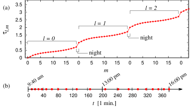
Independently of the day $l$, the KS two-sample test enables us to determine the duration in FST, $\Delta\tau_{m}$ (with $m>0$), of each of the $m_{\rm max}$ partition intervals occurring during a day. For instance, the first 20-minute interval of the day corresponds to $\Delta\tau_{1}=0.08\;\mathrm{fst}$, whereas twenty minutes at half and at the end of the day amount to $\Delta\tau_{11}=0.02\;\mathrm{fst}$ and $\Delta\tau_{19}=0.05\;\mathrm{fst}$, respectively (See Methods for details). Considering the close-to-open return $r_{m_{\rm max},0}^{0,1}$, we can also establish the duration of an overnight interval in the FST: $\Delta\tau_{\rm night}=0.29\;\mathrm{fst}$. Interestingly, the duration of overweekends (Friday-close-to-Monday-open) is about the same. Consistently with the requirement in Eq. (3), the FST scale is hence constructed as

$$\tau_{l,m}\equiv\sum_{n=1}^{m}\Delta\tau_{n}+l\,\left(\sum_{n=1}^{m_{\rm max}}\Delta\tau_{n}+\Delta\tau_{\rm night}\right)\;.$$ (6)

Notice that, assuming Eq. (2), returns over different intervals with the same $\Delta\tau$ are by construction identically distributed.

Figure 2: Empirical PDFs rescaled according to Eq. (1) in (a), and Eq. (2) in (b). While in the physical clock the rescaled PDFs do not satisfy a scaling symmetry since they do not collapse onto each other (a), when proper time is adopted (the FST) the scaling symmetry nicely emerges as rather satisfactory data-collapse (b).

In Fig. 1a we outline the identification of the FST for an equally-spaced partition, $t_{l,m+1}-t_{l,m}=\overline{\Delta t}=20\;{\rm min}$, $m_{\rm max}=19$. The result is obtained by averaging over all possible days in the dataset. Fig. 1a highlights the non-linear character of the FST vs. the physical one. If, reversely, one plots equally-spaced contiguous $\Delta\tau$-intervals as a function of the physical time (Fig. 1b), it becomes evident that the FST runs faster at the beginning and at the end of the day, and slower at noon, New York time.

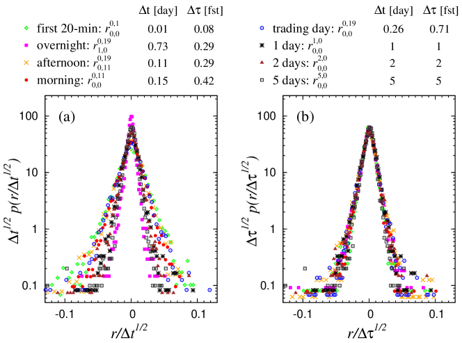
A qualitative inspection about how the FST definition emphasizes the simple scaling properties of the empirical PDFs is offered in Fig. 2 (Tables 1, 2 in the Method Section quantify these results). The comparison of Fig. 2a with Fig. 2b makes evident that only in terms of the FST the data-collapse implied by Eq. (2) can be assumed to hold from 20 min up to several days. As a side note, we observe that both the overnight and the afternoon duration lasts less than the morning interval.

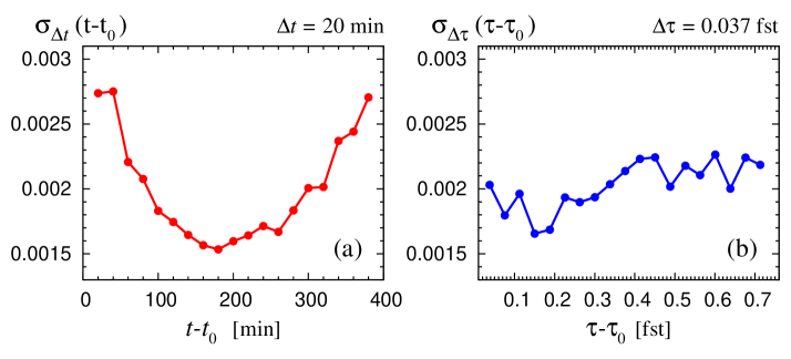
Volatility is a central quantity in financial practice, assessing the intensity of market fluctuations. It may be defined as $\sigma_{\Delta t}(t)\equiv{\mathbb{E}\left[\left|r_{\Delta t}(t)\right|\right]}$ – in FST: $\sigma_{\Delta\tau}(\tau)\equiv{\mathbb{E}\left[\left|r_{\Delta\tau}(\tau)\right|\right]}$. Clear evidence of the nonstationarity of returns in the physical time scale is given by the characteristic “U” shape assumed by the intraday volatility defined over the day-by-day ensemble of returns Bassler et al. (2007); Baldovin et al. (2015); Admati and Pfleiderer (1988); Andersen and Bollerslev (1997) (see Fig. 3a). Once analyzed in terms of FST, volatility stationarity is instead sensibly recovered (Fig. 3b). The availability of a time series with stationary increments, eliminating thus the seasonalities appearing in the physical time scale, conveys the methodological advantage that empirical analyses can be performed through ordinary, sliding-window techniques, hence extending considerably the sample size for statistical confidence.

Figure 3: Intraday volatility. Each market day is assumed to be an independent realization of the same stochastic process Bassler et al. (2007); Baldovin et al. (2015). Volatility over the scale $\Delta t$ (a) and $\Delta\tau$ (b) is plotted as a function of the time elapsing from the market opening ($t_{0}$ and $\tau_{0}$, respectively). While in physical time volatility is markedly nonstationary (a), apart from fluctuations it becomes stationary in FST (b).

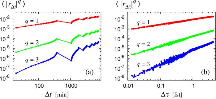
Let us now point out that from Eq. (2) straightforwardly descends $\mathbb{E}\left[|r_{\Delta\tau}|^{q}\right]=(\Delta\tau)^{q/2}\,\int\mathrm{d}x\,g(x)\,|x|^{q}$, or, in the presence of a general Hurst exponent $H$ like in Eq. (1),

$$\mathbb{E}\left[|r_{\Delta\tau}|^{q}\right]=(\Delta\tau)^{qH}\,\int\mathrm{d}x\,g(x)\,|x|^{q}.$$ (7)

One of the consequence of Eq. (7) is that a log-log plot of the $q$th-moment $\mathbb{E}\left[|r_{\Delta\tau}|^{q}\right]$ vs. $\Delta\tau$ should be a straight line with slope $qH$. The empirical analysis of the returns’ moment as a function of the time interval duration is particularly revealing about the meaning of the FST. Fig. 4 highlights that the recurrent patterns deviating from straight behavior in physical time (Fig. 4a) are wiped out in the FST (Fig. 4b).

Figure 4: Empirical moment-analysis. $\Delta t$ (a) and $\Delta\tau$ (b) are the duration of the time intervals over which returns $r_{\Delta t}$ and $r_{\Delta\tau}$ are defined, respectively.

The presence of multiscaling may be easily detected by analyzing the slopes of the log-log plots in Fig. 4. As expected, multiscaling features clearly detectable in physical time (Fig. 5a) are still present but become less pronounced when the FST is adopted (Fig. 5b).

Figure 5: Multiscaling analysis. Slopes of linear regression of the log-log plots in Fig. 4a,b over different ranges of the time interval are respectively reported as a function of the moment-order $q$.

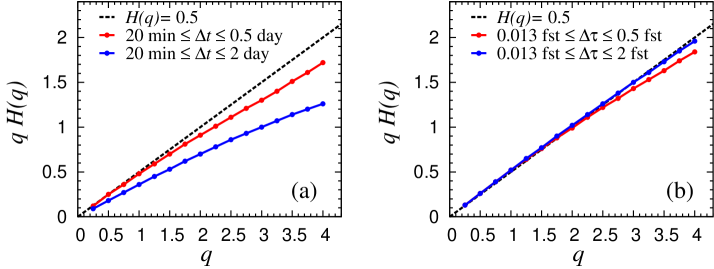
So far, results concern single-point statistics. In Finance, a fundamental two-point indicator is the volatility autocorrelation function Cont (2001); Bouchaud (2003); Dacorogna et al. (2001); Stanley (2000), i.e. the correlation between absolute values of two returns at a given lag. At variance with the linear one, the volatility autocorrelation is known to decay very slowly with the time lag Cont (2001); Bouchaud (2003); Dacorogna et al. (2001); Stanley (2000). In Fig. 6a the $\Delta t=20\;{\rm min}$ volatility autocorrelation at lag $t$, $c_{\sigma,\Delta t}(t)$ Volatility_def , is plotted; while Fig. 6b reports the analogous quantity in FST, $c_{\sigma,\Delta\tau}(\tau)$, for $\Delta\tau=0.037\;{\rm fst}$. In both cases, the autocorrelation has been evaluated through a sliding-window procedure. The ciclostationary quality of $c_{\sigma,\Delta t}(t)$ in physical time is a direct consequence of the “U” shape in Fig. 3a. In contrast, in FST-lag the periodic structure of $c_{\sigma,\Delta\tau}(\tau)$ is almost completely removed, pointing out the methodological advantage in such an empirical estimation.

Figure 6: Volatility autocorrelation as a function of the physical (a) and FST (b) lag. Plots have been realized taking into account all possible pairs of lagged returns in the dataset, with $t$ $(\tau)$ an integer multiple of $\Delta t$ ($\Delta\tau$). The ciclostationary character of the autocorrelation in physical time (a) is suppressed by the adoption of FST (b).

IV Conclusions

We have shown that the adoption as construction criteria of: (i) simple-scaling invariance with Hurst exponent $1/2$ for the return PDF, Eq. (2); (ii) validity of the measure property, Eq.(3); leads to a unique time scale for martingale processes in Finance, which renders stationary the PDFs of returns over identical spans. The construction of FST is based on the minimization of the KS distance of the PDF for the returns at a given scale, with respect to a reference one. It covers a wide range of physical time scales and opens interesting perspectives in the statistical analysis of financial time series. For instance, the attained increments stationarity may sensibly enrich empirical estimates enlarging dataset analyses from ciclostationary to sliding-window procedures. Moreover, we have solved the problem of including overnight and over-weekend returns in financial analysis, bridging intra and interday regimes. This makes markets with discontinuous trading activity closer to those not experiencing transaction interruptions Ghashghaie et. al. (1996), opening thus possibilities for meaningful comparisons.

Methodological approaches based on symmetries are not frequently discussed in Finance. However, some of the ingredients we employed have interesting precursors in the history of financial markets analysis. Indeed, stimulated by the discovery of fat tails Cont (2001); Mantegna and Stanley (1995); Mandelbrot (1963), previous studies Clark (1973); Mandelbrot (1973); Ané et al. (2000) attempted at modifying the returns PDFs through the introduction of a stochastic redefinition of time, in order to cast them into Gaussians. Here, no reference to probability models is made and our FST is not stochastic, but like in these earlier studies our time redefinition is intended to alter some fundamental property of the returns PDFs: in our case, it enforces a simple scaling symmetry. While the distribution of geometric Brownian motion of the standard model of Finance, or the Levy-stable distribution first suggested by Mandelbrot as an alternative Mandelbrot (1963), are invariant under time rescaling, more recent work on financial modeling has focused on multiscaling aspects and their evocative analogies with turbulence Borland et al. (2005); Frisch (1997); Bacry (2008); Mandelbrot (1998).

Along these lines a multifractal operational time has been assumed in the modelization of market evolution and multiscaling has been established as a solid stylized fact in the analysis of series where the interruption are absent or disregarded Bacry (2008); Mandelbrot (1998). One should also mention that the symmetry property expressed by Eq. (1) has been recently assumed as a main modeling ingredient for the stochastic dynamics of financial indexes Baldovin and Stella (2007); Stella and Baldovin (2010); Peirano and Challet (2012); Zamparo et al. (2013); Baldovin et al. (2015). Combining scaling with ideas of fine graining inspired by the renormalization group approach of statistical mechanics Kadanoff (2005), these models reproduce many stylized facts exposed by interday time series analysis, including multiscaling.

As we have shown here our simple scaling ansatz, besides trying to satisfy the exigence of a unique time definition, does not eliminate multiscaling but offers interesting practical advantages. Among these, as discussed in the Methods section with reference to Table 2, is the fact that enforcement of simple scaling appears to result in a better control of stationarity of the whole PDF of returns compared to time definitions related to a single moment.

Our construction, which does not amount to the proposal of a specific parameter dependent model of market dynamics, does not conflict with the possible presence of other stylized facts related to the breaking of time reversal invariance, like the leverage effect Bouchaud et al (2001) whereby a negative price change is on average followed by a volatility increase. Indeed, the FST scale-invariant distribution could, e.g., present skewness.

Time scales capable to conform complex behavior with relatively simple properties shared by ordinary stochastic processes should also be relevant in the study of collective assets dynamics, where time-related issues like e.g. the Epps effect Epps (1979); Renò (2003); Borghesi (2007) or the lead-lag Huth et al. (2000); Curme et al. (2015) question are a main focus of the current research. We believe that strategies similar to the one adopted here could be used in even broader contexts, in cases in which time series display recurrent patterns and scaling properties are at least approximately obeyed. One relevant candidate could be represented by the records of recurrence times Chicheportiche et al. (2014, 2017) either in Finance Bogachev et al. (2007) or in seismicity Corral (2004, 2006).

V Methods

Our FST construction is illustrated considering the S&P500 index recorded in one minute intervals between 9:40 am and 16:00 pm New York time and from 30 September 1985 to 28 June 2013 DataSetStatement . After excluding those days for which the records are not complete (e.g. holidays and market anticipated closures or delayed openings), the data-set includes $L=6852$ trading days. For each single day $l$ ($l=1,\ldots,L$) there is a total of $381$ index values $s(t_{l,n})$ ($n=0,\ldots,N$, with $N=380$). In order to work with zero empirical averages, returns are detrended: $r_{l,n}^{l^{\prime},n^{\prime}}\mapsto r_{l,n}^{l^{\prime},n^{\prime}}-\langle r_{l,n}^{l^{\prime},n^{\prime}}\rangle$, where the average is done over all possible returns with the same $n$, $n^{\prime}$ and same $\Delta l=l^{\prime}-l$, with $t_{l^{\prime},n^{\prime}}>t_{l,n}$. Overnights include single night returns, returns over weekends, returns over holidays and other market closures. Closures due to specific market reasons should be in principle treated differently from weekends and normal holidays (e.g., several days following the black Monday 1987 are missing in the dataset because of anticipated market close). Since we verified that they introduce only minor effects (see also below), in our analysis we do not make such distinctions.

In the construction of $\tau_{l,m}$ a key step consists in checking whether two random variables $X$ and $Y$ are identically distributed. A basic tool to establish this is the KS two-sample test DeGroot (2010); Darling (1957). Given two samples $\left\{x_{i}\right\}_{i=1}^{n_{x}}$, $\left\{y_{i}\right\}_{i=1}^{n_{y}}$, with empirical cumulative distribution functions $F_{x}$, $F_{y}$, respectively, the test is based on the rescaled supremum of the distributions difference:

$$D_{x,y}\equiv\left(\frac{n_{x}\;n_{y}}{n_{x}+n_{y}}\right)^{1/2}\;\sup_{z\in\mathbb{R}}\left\{F_{x}(z)-F_{y}(z)\right\}\,.$$ (8)

In those cases in which the samples refer to independent variables, the test can rely on the KS theorem to assign a significance level to any $D_{x,y}$, under the null hypothesis that $\left\{x_{i}\right\}$, $\left\{y_{i}\right\}$ come from the same distribution. If however samples are extracted from the same time series and data display long-range dependence like in the case examined in the present study, the mapping between $D_{x,y}$ and the associated significance level is expected to be strongly affected Chicheportiche and Bouchaud (2011), and only model-dependent statements can be produced. Still, $D_{x,y}$ quantifies how close the distributions $F_{x}$ and $F_{y}$ are, and here we just employ its minimization in order to determine $\tau_{l,m}$ within a variational strategy.

Table 1: Value of $D_{x,y}$ between different pairs of samples.

	1 night	3 nights	morning	afternoon	trading day	1 day	2 days
first 20 min	10.5	6.54	13.8	12.2	17.2	17.7	18.3
1 night	•	0.82	3.08	2.06	6.58	8.07	10.9
3 nights	•	•	1.77	1.74	3.83	5.25	6.96
morning	•	•	•	1.95	4.09	6.20	9.18
afternoon	•	•	•	•	5.85	7.95	10.4
trading day	•	•	•	•	•	2.81	6.17
1 day	•	•	•	•	•	•	6.96

In Table 1, we report $D_{x,y}$ calculated for different pairs of samples, relative to various intervals in physical time. We emphasize the particularly low value of $D_{x,y}$ if calculated between 1 and and 3 nights. As anticipated, this suggests that it is legitimate to make no distinction between nights and weekends.

Table 2: Outcome of the minimization procedure when the one day open-to-open return distribution is taken as $x$-sample ($n_{x}=6601$, $\Delta\tau_{x}=1\;{\rm fst}$). For $y=10,\;20,\;38\;{\rm min}$, the last two columns correspond in fact to the average of $\Delta\tau_{y}$ and $D_{x,y}$ over the $(380\;{\rm min}/y)$ contiguous time intervals existing within a trading day.

$y$	$n_{y}$	$\Delta\tau_{y}\;[{\rm fst}]$	$D_{x,y}$
10-min	$L$	$0.011$	$1.50$
20-min	$L$	$0.026$	$1.06$
38-min	$L$	$0.054$	$0.87$
morning	$L$	$0.336$	$0.70$
afternoon	$L$	$0.264$	$0.93$
trading day	$L$	$0.682$	$0.64$
overnights	$6601$	$0.213$	$0.82$
2 days	$6350$	$2.150$	$0.61$
3 days	$3235$	$3.308$	$0.79$
5 days	$1187$	$5.633$	$0.75$
10 days	$527$	$10.86$	$1.11$

Table 2 displays the minimal value of $D_{x,y}$ corresponding to the reported value of the FST $\Delta\tau_{y}$, taking as $x$-sample the open-to-open return distribution. While entries for $10$, $20$, $38$ min in Table 2 refer to averages over the whole day of intervals of the respective duration, Fig. 7 details the values of 20-min $\Delta\tau$ from day opening to closure.

Figure 7: Values of 20-min $\Delta\tau$, $\Delta\tau_{m}$ ($m=1,\ldots,19$), from day opening to closure.

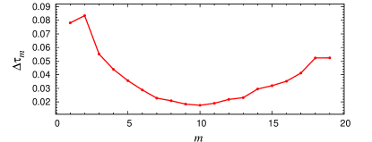
Table 2 clarifies the time-window width where Eq. (2) can be assumed to hold. The $10\;{\rm min}$ interval is the only case with $D_{x,y}$ significantly above $1$. To give a comparison, if in place of the 1-day distribution we take a zero-average Gaussian, the KS analysis returns $D_{x,y}$ values between $1.8$ and $4.2$, with the lower values corresponding to the larger time intervals $y$ as one would expect in accordance with the slow crossover to Gaussianity due to the progressive loss of dependence Cont (2001). It is also worth mentioning that if one computes $D_{x,y}$ rescaling two samples on the basis of their variance or of any specific moment of the PDF, a larger value of $D_{x,y}$ is obtained if compared with the one guaranteed by the KS procedure. Correspondingly, a time scale defined on a single-moment rescaling differs up to $25\%$ with respect to the FST (see Table III in Appendix B). In summary, referring to a single moment for the definition of time is a simpler but less efficient procedure to enforce the stationarity of the whole PDF, since not all information at all price-variation scales is employed.

Figure 8: Empirical linear correlation function between two contiguous intervals of span $\Delta t$.

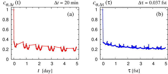
The $10$ min interval is excluded from the FST window not only in view of the large $D_{x,y}$, but also from an analysis of the linear correlations. Let us indicate with $[\Delta t]\equiv\Delta t/(1\;{\rm min})$ the number of minutes characterizing $\Delta t$ (for instance, $[10\;{\rm min}]=10$). The empirical linear correlation between two contiguous intervals of span $\Delta t$ may be calculated as

$$c_{r,\Delta t}(\Delta t) \equiv \frac{1}{{N-2[\Delta t]+1}}\sum_{n=[\Delta t]}^{N-[\Delta t]}\cdot$$

$$\cdot\dfrac{\frac{1}{L}\sum_{l=1}^{L}r^{l,n}_{l,n-[\Delta t]}\,r^{l,n+[\Delta t]}_{l,n}}{\sqrt{\frac{1}{L}\sum_{l=1}^{L}\left(r^{l,n}_{l,n-[\Delta t]}\right)^{2}}\,\sqrt{\frac{1}{L}\sum_{l=1}^{L}\left(r^{l,n+[\Delta t]}_{l,n}\right)^{2}}}\;,$$

and it is plotted in Fig. 8. Linear correlations decrease below our subjective threshold $0.05$ only for $\Delta t>10$ min. Correspondingly, we expect the additive property descending from requirement (ii) to be valid only for intervals duration above such lower bound. With the choice $\overline{\Delta t}=20\;{\rm min}$, we verified that the difference between the measured scaling factor and the one obtained by the additivity rule is always positive (consistently with the positive value of linear correlations) and does not exceed $25$% of the value of the scaling factor. For instance, $\Delta\tau_{\mbox{\scriptsize{1\;day}}}/(\Delta\tau_{\mbox{\scriptsize{morning}}}+\Delta\tau_{\mbox{\scriptsize{afternoon}}}+\Delta\tau_{\mbox{\scriptsize{night}}})\simeq 1.23$.

Appendix A

Here we discuss the limitations posed by multiscaling and simple scaling with Hurst exponent $H\neq 1/2$ to the possibility of defining a univoque time scale able to stationarize the PDF of returns and obeying natural additivity properties.

In the presence of multiscaling, $q$-order moments must obey the general expression

$$\mathbb{E}\left[|r|^{q}\right]=A_{q}\Delta t^{qH(q)}\;,$$ (10)

where $r$ are the returns in an interval of duration $\Delta t$, $A_{q}$ is a generic $q$-dependent amplitude and also the Hurst exponent becomes a function of $q$.

A natural strategy towards stationarization of the returns over equal time span is that of defining a time scale based on the choice of a particular moment-order $q$. If we indicate by $r$ the returns in an interval of duration $\Delta t$ and by $r_{0}$ the returns in an interval of duration $\Delta t_{0}$ (in our work we chose $\Delta t_{0}=1$ day), the new time duration $\Delta\tau(q)$ of a generic interval $\Delta t$ can be defined as

$$\Delta\tau(q)\equiv\dfrac{\mathbb{E}\left[|r|^{q}\right]^{\frac{2}{q}}}{\mathbb{E}\left[|r_{0}|^{q}\right]^{\frac{2}{q}}}\;.$$ (11)

Notice that in the case of a Wiener process, for which Eq. (2) is strictly valid with a Gaussian $g$, the new time does not depend on $q$ and is equivalent to the physical time.

However, from Eq. (10) and (11) one obtains

$$\Delta\tau(q)=\left(\dfrac{\Delta t}{\Delta t_{0}}\right)^{2H(q)}\;.$$ (12)

This immediately implies that this time definition is $q$-independent only if $H(q)$ is constant (no multiscaling). One could easily prove also the converse argument. Namely, that no $q$-independent time redefinition can completely eliminate the existence of nontrivial multiscaling effects.

Furthermore the time defined by Eq. (11) is not additive unless $H=1/2$. Indeed, consider $r_{1}$ and $r_{2}$ as the returns of two successive contiguous intervals $\Delta t_{1}$ and $\Delta t_{2}$ with $\Delta t=\Delta t_{1}+\Delta t_{2}$ and $r=r_{1}+r_{2}$ as their aggregate, then, with $H\neq 1/2$ we have

$$\Delta\tau_{1}(q)+\Delta\tau_{2}(q)\neq\Delta\tau(q)\;,$$ (13)

where $\Delta\tau$, $\Delta\tau_{1}$ and $\Delta\tau_{2}$ are the new time duration respectively associated to the PDF of $r$, $r_{1}$ and $r_{2}$.

The above considerations are at the basis of our ansatz scheme which assumes the validity of Eq. (2) as the starting point to construct FST as an additive time independent of moment order.

Appendix B

To better clarify the differences between fst and a time scale constructed starting from Eq. (11), we report in Table 3 the outcome of different moment $q$ choices.

Table 3: Outcome of a time definition procedure when the one day open-to-open return distribution is taken as $x$-sample. For $y=10,\;20,\;38\;{\rm min}$, the last two columns correspond in fact to the average of $\Delta\tau_{y}$ and $D_{x,y}$ over the $(380\;{\rm min}/y)$ contiguous time intervals existing within a trading day. Columns with “fst” title report data already presented in Table 2 coming from the KS minimization procedure while the other colums are obtained for a time definition based on a single moment $q$; see Eq. (11).

	fst		$q=1$		$q=2$		$q=3$
$y$	$\Delta\tau_{y}$	$D_{x,y}$	$\Delta\tau_{y}$	$D_{x,y}$	$\Delta\tau_{y}$	$D_{x,y}$	$\Delta\tau_{y}$	$D_{x,y}$
10-min	$0.011$	$1.50$	$0.013$	$2.26$	$0.015$	$2.83$	$0.014$	$2.77$
20-min	$0.026$	$1.06$	$0.031$	$2.26$	$0.031$	$1.90$	$0.032$	$2.12$
38-min	$0.054$	$0.87$	$0.066$	$1.38$	$0.061$	$1.52$	$0.069$	$1.84$
morning	$0.336$	$0.70$	$0.347$	$0.81$	$0.325$	$0.82$	$0.264$	$1.99$
afternoon	$0.264$	$0.93$	$0.305$	$1.57$	$0.353$	$2.38$	$0.392$	$3.00$
trading day	$0.682$	$0.64$	$0.707$	$0.87$	$0.733$	$1.06$	$0.784$	$1.47$
overnights	$0.213$	$0.82$	$0.238$	$1.24$	$0.248$	$1.41$	$0.214$	$0.86$
2 days	$2.150$	$0.61$	$2.074$	$0.64$	$2.164$	$0.62$	$2.294$	$0.87$
3 days	$3.308$	$0.79$	$3.033$	$1.00$	$2.889$	$1.09$	$2.755$	$1.24$
5 days	$5.633$	$0.75$	$5.186$	$0.91$	$4.946$	$1.00$	$4.724$	$1.12$
10 days	$10.86$	$1.11$	$9.318$	$1.13$	$9.615$	$1.13$	$9.541$	$1.11$

Results show that a time definition based on the second moment may differ up to about 25 % with respect to our fst, defined via the Kolmogorov-Smirnov test and that time scales defined on the other considered moments ($q=1,3$) do not perfom better as far as KS distance is concerned. Furthermore the Table shows that, to define a time scale which enforces the scaling symmetry Eq. (2), there is not a preferential moment since the best choice would depend on the considered time interval. For example in the case of overnight returns a time definition based on the third moment would perform much better in the attempt to satisfy Eq. (2). This shows that if the goal is to promote in the best possible way the stationarity of the return pdf’s (and this is our goal), the KS criterion on which we rely in our procedure is much more adequate than any moment based procedure.

References

- Wald (1984) See, e.g., R.M. Wald, General Relativity (University of Chicago Press, 1984).
- Ivanova et al. (1999) K. Ivanova and M. Ausloos, Physica A 274, 349 (1999).
- Corral (2004) Á. Corral, Phys. Rev. Lett. 92, 108501 (2004).
- Corral (2006) Á. Corral, Lecture notes in Physics 705, 191 (2006).
- Peng et al. (1995) C.-K. Peng, S. Havlin, H. E. Stanley, and A. L. Goldberger, Chaos 5, 82 (1995).
- Peng et al. (2001) Y. Ashkenazy, P. Ch. Ivanov, S. Havlin, Chung-K. Peng, A. L. Goldberger, and H. E. Stanley, Phys. Rev. Lett. 86, 1900 (2001).
- Hausdorff et al. (1995) J. M. Hausdorff, C.-K. Peng, Z. Ladin, J. Wei, and A. L. Goldberger, J. Appl. Physiol. 78, 349 (1995).
- Liu et al. (1997) Y. Liu, P. Cizeau, M. Meyer, C.-K. Peng, and H. E. Stanley, Physica A 245, 437 (1997).
- Galluccio et al. (1997) S. Galluccio, G. Caldarelli, M. Marsili, and Y.-C. Zhang, Phys. A 245, 423 (1997).
- Bassler et al. (2007) K. E. Bassler, J. L. McCauley, and G. H. Gunaratne, Proc. Natl. Acad. Sci. U.S.A. 104, 17287 (2007).
- Tsay (2002) R.S. Tsay, Analysis of Financial Time Series (John Wiley & Sons, New York, 2002).
- Peng et al. (1994) C.-K. Peng, S. V. Buldyrev, S. Havlin, M. Simons, H. E. Stanley, and A. L. Goldberger, Phys. Rev. E. 49, 1685 (1994).
- Kantelhardt et al. (2002) J. W. Kantelhardt, S. A. Zschiegner, E. Koscielny-Bunde, A. Bunde, S. Havlin, and H. E. Stanley, Physica A 316, 87 (2002).
- Chen et al. (2002) Z. Chen, P. Ch. Ivanov, K. Hu, and H. E. Stanley, Phys. Rev. E. 65, 041107 (2002).
- Bryce et al. (2012) R. M. Bryce and K. B. Sprague, Scient. Rep. 2, 315 (2012).
- Dacorogna et al. (1996) M.M. Dacorogna, C.L. Gauvreau, U.A. Müller, R.B. Olsen, O.V. Pictet, J. Forecasting 15, 203 (1996).
- Dacorogna et al. (2001) M.M. Dacorogna, R. Gençay, U.A. Müller, R.B. Olsen, O.V. Pictet, An Introduction to High-frequency Finance (Academic Press, San Diego, 2001).
- Zumbach (2002) G. Zumbach, in Econophysics: An Emergent Science. Proceedings of the 1st Workshop on Econophysics, Budapest, 1997 (ed. J. Kertész and I. Kondor http://newton.phy.bme.hu/ kullmann/Egyetem/toc.html, Budapest, 2002).
- Omori (1984) F. Omori, J. Coll. Sci. Imp. Univ. Tokyo 7, 111 (1984).
- Gardner et al. (2006) W. A. Gardner, A. Napolitano, and L. Paura, Signal Processing 86, 639 (2006).
- Calvet and Fischer (2002) L. Calvet and A. Fischer, The Rev. of Econom. and Stat. LXXXIV, 381 (2002).
- Borland et al. (2005) L. Borland, J.-P. Bouchaud, J.-F. Muzy, and G. Zumbach, Wilmott Magazine , (2005).
- Di Matteo (2007) T. Di Matteo, Quant. Fin. 7, 21 (2007).
- Frisch (1997) U. Frisch, Turbulence: The Legacy of A. Kolmogorov (Cambridge University Press, Cambridge, 1997).
- Bacry (2008) E. Bacry, A. Kozhemyak, J.F. Muzy, Journ. Econ. Dyn. and Control 32, 156 (2008).
- Mandelbrot (1998) B.B. Mandelbrot, L. Calvet, A. Fisher, Cowles Foundation Discussion Paper 1164, 156 (1998).
- Bogachev et al. (2007) M.I. Bogachev, and J.F. Eichner, and A. Bunde, Phys. Rev. Lett. 99, 240601 (2007).
- Chicheportiche et al. (2014) R. Chicheportiche, and A. Chakraborti, Phys. Rev. E. 89, 042117 (2014).
- Chicheportiche et al. (2017) R. Chicheportiche, and A. Chakraborti, Phys. A , In Press (2017).
- Clark (1973) P. K. Clark Econometrica 41, 135 (1973).
- Ané et al. (1999) T. Ané and H. Geman, J. Risk 1, 57 (1999).
- Stanley (2000) R.-N. Mantegna and H. E. Stanley, Introduction to Econophysics: Correlations and Complexity in Finance (Cambridge University Press, Cambridge, 2000).
- Jensen et al. (2004) M. H. Jensen, A. Johansen, F. Petroni, and I. Simonsen, Physica A 340, 678 (2004).
- Gillemot et al. (2006) L. Gillemot, J.D. Farmer, and F. Lillo, Quant. Fin 6, 371 (2006).
- Baldovin and Stella (2007) F. Baldovin and A. L. Stella, Proc. Natl. Acad. Sci. USA 104, 19741 (2007).
- Hurst (1951) H. E. Hurst Trans. Am. Soc. Civil Eng. 116, 770 (1951).
- Di Matteo et al. (2005) T. Di Matteo, T. Aste, and M. M Dacorogna, J. Bank & Fin. 29, 827 (2005).
- Allez et al. (2011) R. Allez and J. P. Bouchaud, New J. Phys. 13, 025010 (2011).
- Baldovin et al. (2015) F. Baldovin, F. Camana, M. Caporin, M. Caraglio, and A. L. Stella, Quant. Fin. 15, 231 (2015).
- Cont (2001) R. Cont, Quant. Fin. 1, 223 (2001).
- Wang et al. (2015) F. Wang, K. Yamasaki, K. Havlin, and H.E. Stanley, Phys. Rev. E 77, 016109 (2008).
- Bouchaud (2003) J.-P. Bouchaud and M. Potters, Theory of Financial Risk and Derivative Pricing (Cambridge University Press, Cambridge, 2003).
- DeGroot (2010) M. H. DeGroot and M. J. Schervish, Probability and Statistics (4th ed.) (Addison-Wesley, Boston, 2010).
- Darling (1957) D. A. Darling, Ann. Math. Stat. 28, 823 (1957).
- (45) Whereas New York market opens at 9:30 am, our dataset records start instead at 9:40 am.
- Admati and Pfleiderer (1988) A. Admati and P. Pfleiderer, Rev. Financ. Stud. 1, 3 (1988).
- Andersen and Bollerslev (1997) T. G. Andersen and T. Bollerslev, J. Empir. Finance 4, 115 (1997).
- (48) The volatility autocorrelation is defined as where is a sliding-window empirical average with respect to , performed over all available couples in the dataset. An analogous definition follows for in FST.
- Ghashghaie et. al. (1996) S. Ghashghaie, W. Breymann, J. Peinke, P. Talkner, and Y. Dodge, Nature 381, 767 (1996).
- Mantegna and Stanley (1995) R. Mantegna and H.E. Stanley, Nature 376, 46 (1995).
- Mandelbrot (1963) B. Mandelbrot, J. Business XXXVI, 392 (1963).
- Mandelbrot (1973) B. B. Mandelbrot, Econometrica 41, 157 (1973).
- Ané et al. (2000) T. Ané, and H. Geman, Journ. Fin. 55, 2259 (2000).
- Stella and Baldovin (2010) A. L. Stella and F. Baldovin, J. Stat. Mech., P02018 (2010).
- Peirano and Challet (2012) P. P. Peirano and D. Challet, Eur. Phys. J. B. 85, 276 (2012).
- Zamparo et al. (2013) M. Zamparo, F. Baldovin, M. Caraglio, and A. L. Stella, Phys. Rev. E 88, 062808 (2013).
- Baldovin et al. (2015) F. Baldovin, M. Caporin, M. Caraglio, A. L. Stella, and M. Zamparo, J. Econom. 187, 486 (2015).
- Kadanoff (2005) L.P. Kadanoff, Statistical Physics, Statics, Dynamics and Renormalization (World Scientific, Singapore, 2005).
- Bouchaud et al (2001) J.-P. Bouchaud, A. Matacz, M. Potters, Phys. Rev. Lett. 87, 228701 (2001).
- Epps (1979) T.W. Epps, Journ. Am. Stat. Ass. 74, 291 (1979).
- Renò (2003) R. Renò, Int. J. Theor. Appl. Finance 6, 87 (2003).
- Borghesi (2007) C. Borghesi, M. Marsili, S. Miccichè, Phys. Rev. E 76, 026104 (2007).
- Huth et al. (2000) N. Huth, and F. Abergel, J. Emp. Fin. 26, 41 (2014).
- Curme et al. (2015) C. Curme, M. Tumminello, R. N. Mantegna, H. E. Stanley, and D. Y. Kenett, Quant. Fin. 15, 1375 (2015).
- Chicheportiche and Bouchaud (2011) R. Chicheportiche and J.-P. Bouchaud, J. Stat. Mech., P09003 (2011).