The second law of thermodynamics from symmetry and unitarity

Abstract

The second law of thermodynamics states that for a thermally isolated system entropy never decreases. Most physical processes we observe in nature involve variations of macroscopic quantities over spatial and temporal scales much larger than microscopic molecular collision scales and thus can be considered as in local equilibrium. For a many-body system in local equilibrium a stronger version of the second law applies which says that the entropy production at each spacetime point should be non-negative. In this paper we provide a proof of the second law for such systems and a first derivation of the local second law. For this purpose we develop a general non-equilibrium effective field theory of slow degrees of freedom from integrating out fast degrees of freedom in a quantum many-body system and consider its classical limit. The key elements of the proof are the presence of a $Z_{2}$ symmetry, which can be considered as a proxy for local equilibrium and micro-time-reversibility, and a classical remnant of quantum unitarity. The $Z_{2}$ symmetry leads to a local current from a procedure analogous to that used in the Noether theorem. Unitarity leads to a definite sign of the divergence of the current. We also discuss the origin of an arrow of time, as well as the coincidence of causal and thermodynamical arrows of time. Applied to hydrodynamics, the proof gives a first-principle derivation of the phenomenological entropy current condition and provides a constructive procedure for obtaining the entropy current.

I Introduction

Ink dropped into a bowl of water spreads and does not regroup, a broken toy does not reassemble itself, heat does not pass spontaneously from a cooler to a hotter object; such irreversible phenomena are ubiquitous in nature. They are explained by the second law of thermodynamics, which associates a physical quantity called entropy with an equilibrium state of matter and states that for a thermally isolated system entropy never decreases. Heuristically speaking, entropy is a measure of manifest disorder. Ink molecules spreading uniformly in water is more disordered than concentrated in a single drop and thus has a higher entropy. The second law governs essentially all aspects of the universe, from molecular dynamics to star formations, from engines to biological systems, from cosmology to black holes and quantum gravity.

For many physical processes in nature, in fact a stronger version of the second law is in operation. Typical physical processes we observe involve variations of macroscopic quantities over spatial and temporal scales much larger than microscopic molecular collision scales. Thus for any region $V$ whose size is much larger than molecular scales but much smaller than the distance and time scales of variations can be considered as in local equilibrium. Going to a continuum description we can then introduce an entropy density $s(t,\vec{x})$ and an entropy flow vector $S^{i}$, to express the second law in a local form as

$$\partial_{t}\int_{V}d^{3}\vec{x}\,s(t,{\vec{x}})+\int_{\partial V}d\vec{\sigma}\cdot\vec{S}\geq 0,\quad\Rightarrow\quad\partial_{\mu}S^{\mu}\geq 0,\quad S^{\mu}=(s,S^{i})$$ (1)

We emphasize that local equilibrium does not mean near equilibrium as variations of macroscopical physical quantities can be big over large distances and long time periods, and in fact includes most far-from-equilibrium situations observed in nature.

While the second law was first formulated by Clausius more than one and a half centuries ago, understanding how it arises from basic laws of physics which are time symmetric, remains incomplete. In particular, while the local second law has played a central role in formulating many phenomenological theories including fluid mechanics LL , there has not been any derivation of it from first principle.

In this paper we provide a proof of the second law and the local second law (1) for the classical limit of any quantum many-body system in local equilibrium. The second law is proved in general while the local version is proved perturbatively in a derivative expansion. The basic idea is as follows. We start by formulating a general non-equilibrium effective field theory for a quantum many-body system obtained by integrating out fast degrees of freedom. Interestingly, unitarity of quantum time evolution imposes various constraints on the action which survive in the classical limit. For example, the action is in general complex and the imaginary part of the action is non-negative. We then impose a $Z_{2}$ symmetry janssen1 ; janssen2 ; Sieberer2 ; CGL ; CGL1 , which can be considered as a proxy for local equilibrium and micro-time-reversibility. It implies that the first law of thermodynamics, Onsager relations, as well as fluctuation-dissipation relations are satisfied locally. From a procedure analogous to that in the proof of Noether’s theorem, the $Z_{2}$ symmetry leads to a local current which is not conserved, but whose divergence can be expressed in terms of the imaginary part of the action, and is thus non-negative. At zeroth order in derivative expansion the current is conserved and recovers the standard thermodynamic entropy. We also discuss the origin of the arrow of time which can be attributed to whether the local equilibrium is established in the past or in the future.

Our proof of the second law complements the existing proofs and brings a number of immediate conceptual implications. The celebrated Boltzmann’s H theorem boltz applies to dilute gases, and the fluctuation theorems boch ; jarz1 ; crooks apply to classical Hamiltonian systems initially in thermal equilibrium perturbed by external mechanical forces. Ours applies to all systems in local equilibrium including liquids, critical systems, and quantum liquids such as superfluids and strongly correlated systems. While the H-theorem starts with a statistical definition of entropy, here the concept of thermodynamical entropy is emergent, arising from a $Z_{2}$ symmetry. The derivation only shows that there is a monotonic quantity, which turns out to coincide with our usual notion of thermodynamic entropy. Our derivation also highlights the importance of quantum unitarity in the monotonicity of entropy evolution. It implies that if one just writes down a most general classical effective action for a dissipative open system, entropy evolution may not be monotonic.

As with earlier derivations boltz ; boch ; jarz1 ; crooks , here a thermodynamic arrow of time arises with a choice of boundary condition in time. Without such an extra input the most one could get from an underlying time-symmetric system is the monotonicity of entropy evolution. Also as in other derivations microscopic time reversibility plays a key role.

Applied to the hydrodynamical action recently proposed in CGL ; CGL1 , our derivation of the local second law (1) gives a first-principle derivation of the phenomenological entropy current condition and a constructive procedure for obtaining the entropy current. Recent advances in understanding the entropy current condition in hydrodynamics include Banerjee:2012iz ; Jensen:2012jh ; Bhattacharyya:2013lha ; Bhattacharyya:2014bha . At ideal fluid level, entropy current arises as a topologically conserved current in the formulation of Dubovsky:2011sj ; Dubovsky:2005xd , while in deBoer:2015ija ; CGL it arises as the Noether current for an accidental continuous symmetry. In Haehl:2015pja entropy current is proposed at non-dissipative level as the Noether current associated to a $U(1)$ symmetry, which was further advocated in Haehl:2015uoc as a symmetry for full dissipative fluids.

The plan of the paper is as follows. In next section we formulate a general class of non-equilibrium effective field theories. We discuss constraints from unitarity and introduce a $Z_{2}$ symmetry to impose local equilibrium. In Sec. III we present a proof of the second law and a perturbative proof of its local second version. We conclude in Sec. IV with a discussion of the origin of an arrow of time. We have included a number of appendices which contain explicit examples as well as various background materials and technical details.

II Non-equilibrium effective theories

In this section we formulate a most general non-equilibrium effective theory obtained from consistently integrating out “fast” degrees of freedom in a state of local equilibrium. By fast degrees of freedom we mean either gapped modes or modes with a finite lifetime in the long wavelength limit (which can include gapless modes). This means that there is a separation of scales between the integrated-out fast and remaining “slow” degrees of freedom, and thus the effective action for the slow modes must be local, i.e. has a regular local expansion in terms of the number of derivatives. The expansion in derivatives is controlled by a small parameter $\epsilon/L\ll 1$ where $L$ is the characteristic wavelength (or inverse frequency) of the slow degrees of freedom while $\epsilon$ is some microscopic scale characterizing the life-times and correlation lengths of fast degrees of freedom.

Consider the path integral for describing expectation values in a quantum state, which can be defined on a closed time path (CTP) contour schwinger ; keldysh ; Feynman:1963fq ,

$$e^{W[\phi_{1},\phi_{2}]} =\mathop{\rm Tr}\left(U(+\infty,-\infty;\phi_{1})\rho_{0}U^{\dagger}(+\infty,-\infty;\phi_{2})\right)=\int_{\rho_{0}}D\psi_{1}D\psi_{2}\,e^{iS_{0}[\psi_{1},\phi_{1}]-iS_{0}[\psi_{2};\phi_{2}]}$$ (2)

where $\rho_{0}$ denotes the initial state of the system, and $U(t_{2},t_{1};\phi)$ is the evolution operator of the system from $t_{1}$ to $t_{2}$ in the presence of external sources collectively denoted by $\phi$. The sources are taken to be slowly varying functions and there are two copies of them, one for each leg of the CTP contour. The second equality is the “microscopic” path integral description, with $\psi_{1,2}$ denoting microscopic dynamical variables for the two copies of spacetime of the CTP and $S_{0}[\psi;\phi]$ the microscopic action. Now suppose in this system there is a natural separation of slow and fast degrees of freedom and integrate out fast variables, after which

$$e^{W[\phi_{1},\phi_{2}]}=\int D\chi_{1}D\chi_{2}\,e^{iI_{\rm eff}[\chi_{1},\phi_{1};\chi_{2},\phi_{2};\rho_{0}]}\$$ (3)

where $\chi_{1,2}$ denote slow variables and there are again two copies of them. It is convenient to introduce the so-called $r-a$ variables Chou:1984es

$$\chi_{r}={{\frac{1}{2}}}(\chi_{1}+\chi_{2}),\quad\chi_{a}=\chi_{1}-\chi_{2},\quad\phi_{r}={{\frac{1}{2}}}(\phi_{1}+\phi_{2}),\quad\phi_{a}=\phi_{1}-\phi_{2}\$$ (4)

where as usual $\chi_{r}$ correspond to physical observables while $\chi_{a}$ correspond to noises.

Unitarity of time evolution in (2) imposes nontrivial constraints on $I_{\rm eff}$. Taking the complex conjugate of (2) we find that $W$ satisfies $W^{*}[\phi_{1},\phi_{2}]=W[\phi_{2},\phi_{1}]$ which in turn requires that

$$I^{*}_{\rm eff}[\chi_{r},\phi_{r};\chi_{a},\phi_{a}]=-I_{\rm eff}[\chi_{r},\phi_{r};-\chi_{a},-\phi_{a}]\$$ (5)

where for definiteness we have taken $\chi_{1,2}$ and sources $\phi_{1,2}$ to be real. Equation (5) implies that terms in $I_{\rm eff}$ which are even in $a$-variables must be pure imaginary. Note that the original factorized form of the action in (2) is real and is odd in $a$-variables. Given that one expects even terms will generically be generated when integrating out fast variables, $I_{\rm eff}$ is thus generically complex. Now that $iI_{\rm eff}$ can be real, there is a danger that the integrand of (3) can be exponentially increasing with $\chi_{1,2}$ thus making the path integrals ill-defined. Note, however, that unitarity of evolution operator $U$ implies

$${\rm Im}\,I_{\rm eff}\geq 0\$$ (6)

for any dynamical variables $\chi_{1,2}$ and sources $\phi_{1,2}$. There is one further constraint from unitarity: in (2) taking $\phi_{1}=\phi_{2}=\phi$ and $\chi_{1}=\chi_{2}=\chi$, we should have

$$I_{\rm eff}[\chi,\phi;\chi,\phi]=0,\quad{\rm or}\quad I_{\rm eff}[\chi_{r}=\chi,\phi_{r}=\phi;\chi_{a}=0,\phi_{a}=0]=0\ .$$ (7)

Equation (7) implies that any term in the action must contain at least one factor of $a$-type variables ($\phi_{a}$ or $\chi_{a}$). We give a derivation of (5)–(7) in Appendix A.

There are three different regimes for (3). The first is the full quantum level where path integrations describe both quantum and classical statistical fluctuations. The second is the classical limit with $\hbar\to 0$ where the path integrals remain and describe classical statistical fluctuations. The third is the level of equations of motion from $I_{\rm eff}$ which corresponds to the thermodynamic limit with all classical and quantum fluctuations neglected. The consequences (5)–(7) of quantum unitarity concern with general structure of $I_{\rm eff}$ and thus survive in all regimes. In this paper we will work at the level of equations of motion.

It is straightforward to write down the most general effective action $I_{\rm eff}$ for slow modes corresponding to non-conserved quantities. For hydrodynamic modes associated with conserved quantities such as the energy-momentum tensor or charges of some internal symmetries, the problem is much trickier both in terms of identifying the appropriate dynamical variables $\chi$ and the symmetries that $I_{\rm eff}$ should obey, and has only been recently solved in CGL ; CGL1 (see also Dubovsky:2005xd ; Dubovsky:2011sj ; Grozdanov:2013dba ; Kovtun:2014hpa ; Harder:2015nxa ; Haehl:2015uoc for other recent discussions). Here we follow the formulation of the classical limit in CGL1 . For definiteness, let us consider a system with a $U(1)$ symmetry. The most general Lagrangian density for $I_{\text{eff}}=\int d^{d}x\,\mathcal{L}_{\text{eff}}$, including both non-conserved and hydrodynamic modes can be written as

$${{\mathcal{L}}}_{\rm eff}=\sum_{n=1}^{\infty}i^{\eta_{n}}f^{(n)}[\Lambda_{r}]\Phi_{a}^{n},\qquad\eta_{n}=\begin{cases}1&n\;{\rm even}\cr 0&n\;{\rm odd}\end{cases}\$$ (8)

where $\Lambda_{r}$ denotes the collection of $r$-variables while $\Phi_{a}$ denotes the collection of $a$-variables. The $n$-th term in (8) should be understood as

$$f^{(n)}[\Lambda_{r}]\Phi_{a}^{n}=f^{(n)}_{{\alpha}_{1}\cdots{\alpha}_{n}}(\Lambda_{r};\partial_{\mu})\,\Phi_{a{\alpha}_{1}}(x)\cdots\Phi_{a{\alpha}_{n}}(x)\$$ (9)

where $f^{(n)}_{{\alpha}_{1}\cdots{\alpha}_{n}}(\Lambda_{r};\partial_{\mu})$ is a function of $\Lambda_{r}$, their derivatives, as well as derivative operators acting on $\Phi_{a{\alpha}}$, with index ${\alpha}$ running over different $a$-variables. In (8) the sum starts at $n=1$ due to (7) and the even terms are pure imaginary due to (5). While in practice one only needs to keep the first few terms in (8) in powers of $a$-variables and derivatives, here we keep the full dependence for both. More explicitly, we can write $\Lambda_{r}=\{\chi_{r{\rm i}},\beta^{\mu},{\hat{\mu}}\}$ and $\Phi_{a}=\{\chi_{a{\rm i}},\partial_{\mu}X_{a\nu},\partial_{\mu}\varphi_{a}\}$, where $\chi_{r{\rm i}},\chi_{a{\rm i}}$ denote slow variables for non-conserved quantities with index ${\rm i}$ labeling different species. $\beta^{\mu}=\beta(x)u^{\mu}(x)$ and ${\hat{\mu}}=\beta(x)\mu(x)$ are hydrodynamical $r$-variables where $\beta(x),u^{\mu},\mu(x)$ are respectively local inverse temperature, local velocity field and local chemical potential. Hydrodynamical $a$-variables $X_{a}^{\mu},\varphi_{a}$ correspond to noises for the energy-momentum and the $U(1)$ charge, and must always be accompanied by derivatives as already indicated in $\Phi_{a}$. In particular, in derivative expansion, $\partial_{\mu}X_{a\nu},\partial_{\mu}\varphi_{a}$ should be counted as having zero derivatives. For definiteness we use the relativistic regime throughout the paper. For a non-relativistic system the discussion is completely parallel.

Let us now turn to equations of motion of $I_{\rm eff}$. Given that (8) contains at least one factor of $\Phi_{a}$, equations of motion from varying with respect to any $r$-variables can be consistently solved by setting all $a$-variables to zero. Thus nontrivial equations of motion come from varying with respect to $a$-variables and furthermore only $f^{(1)}$ are relevant. More explicitly let us write

$$f^{(1)}[\Lambda_{r}]\Phi_{a}=E_{{\rm i}}\chi_{a{\rm i}}+T^{\mu\nu}\partial_{\mu}X_{a\nu}+J^{\mu}\partial_{\mu}\varphi_{a}$$ (10)

where by using integration by parts we can move all derivatives on $\Phi_{a}=\{\chi_{a{\rm i}},\partial_{\mu}X_{a\nu},\partial_{\mu}\varphi_{a}\}$ to the other factors. Thus the equations of motion can be written as

$$E_{{\rm i}}=0,\qquad\partial_{\mu}T^{\mu\nu}=0,\qquad\partial_{\mu}J^{\mu}=0\ .$$ (11)

$T^{\mu\nu}$ and $J^{\mu}$ can be interpreted as the (macroscopic) energy momentum tensor and $U(1)$ current, and the second and third equations are simply the corresponding conservation equations. In Appendix D we discuss two explicit examples, model A for critical dynamics and fluctuating hydrodynamics for a relativistic charged fluid.

We now impose a $Z_{2}$ symmetry, to which we will refer as the dynamical KMS symmetry. More explicitly we require that

$$I_{\rm eff}[\Lambda_{r},\Phi_{a}]=I_{\rm eff}[\tilde{\Lambda}_{r},\tilde{\Phi}_{a}]$$ (12)

where in the classical limit $\hbar\to 0$

$$\tilde{\Lambda}_{r}(-x)=\Lambda_{r}(x),\qquad\tilde{\Phi}_{a}(-x)=\Phi_{a}(x)+i\Phi_{r}(x)$$ (13)

with $\Phi_{r}=\{\beta^{\mu}\partial_{\mu}\chi_{r{\rm i}},\partial_{\mu}\beta_{\nu},\partial_{\mu}{\hat{\mu}}\}$ respectively for $\Phi_{a}=\{\chi_{a{\rm i}},\partial_{\mu}X_{a\nu},\partial_{\mu}\varphi_{a}\}$. The dynamical KMS symmetry plays the role of imposing micro-time-reversibility and local equilibrium. In Appendix B we elaborate more on their motivations and in Appendix D we illustrate their physical implications using some examples. For non-conserved quantities $\chi_{r{\rm i}},\chi_{a{\rm i}}$ the transformation (13) generalizes to local equilibrium a previously known transformation characterizing a thermal ensemble janssen1 ; janssen2 ; Sieberer2 . Those for hydrodynamical variables have only been recently proposed in CGL ; CGL1 . The transformations (13), to which we will refer as dynamical KMS transformations below, are $Z_{2}$. This is obvious for $\Lambda_{r}$. For $\Phi_{a}$, we have

$$\tilde{\tilde{\Phi}}_{a}=\tilde{\Phi}_{a}(-x)+i\tilde{\Phi}_{r}(-x)=\Phi_{a}(x)+i\Phi_{r}(x)-i\Phi_{r}(x)=\Phi_{a}(x)$$ (14)

where we have used that $\tilde{\Phi}_{r}(-x)=-\Phi_{r}(x)$ due to the single derivative inside $\Phi_{r}$.

Since $\Phi_{r}$ contains one derivative, the dynamical KMS condition (12) relate $n$-th derivative terms in $f^{(1)}$ with $(n-1)$-th derivative terms in $f^{(2)}$, $(n-2)$-th derivative terms in $f^{(3)}$, etc., all the way to zeroth derivative terms in $f^{(n)}$. Thus even though the equations of motion (11) only involve $f^{(1)}$, all terms in (8) play a role through (12). Also note that the zero derivative part of $f^{(1)}$ should be invariant by itself, which we will see have interesting implications.

One can include external sources in (8). For $\phi_{1}=\phi_{2}=\phi$, i.e. $\phi_{r}=\phi,\phi_{a}=0$ one can simply replace $f^{(n)}$ in (8) by $f^{(n)}[\Lambda_{r},\phi]$, i.e. now becoming also local functions of $\phi$ and their derivatives. Turning on $\phi_{r}$ for the stress tensor corresponds to putting the system on a curved spacetime metric $g_{\mu\nu}$ in which case one should replace all derivatives by covariant derivatives associated with $g_{\mu\nu}$. Also note that the dynamical KMS transformation for $\phi$ is $\tilde{\phi}_{r}(-x)=\phi_{r}(x)$. We will not need to turn on $\phi_{a}$ for this paper.

III A theorem of local second law of thermodynamics

In this section we will prove a general theorem on the second law of thermodynamics.

Theorem: for any local effective theory (8) which satisfies (6) and the $Z_{2}$ dynamical KMS symmetry (12) there exists a local density $S^{0}$ which satisfies (given equations of motion)

$$\Delta S\equiv\int_{t=t_{2}}d^{d-1}x\,S^{0}-\int_{t=t_{1}}d^{d-1}x\,S^{0}\geq 0\ .$$ (15)

Furthermore perturbatively to all orders in derivative expansion there exists a local current $S^{\mu}$ satisfying

$$\partial_{\mu}S^{\mu}\geq 0\ .$$ (16)

Denote $S^{\mu}_{0}$ as the expression for $S^{\mu}$ at zeroth order in derivative expansion, then

$$\partial_{\mu}S^{\mu}_{0}=0\$$ (17)

and recovers the standard equilibrium thermodynamical entropy. The theorem can be straightforwardly generalized to include diagonal external sources $\phi$. In particular, in a curved spacetime metric $g_{\mu\nu}$ one should replace the derivatives in (16) and (17) by covariant derivatives associated with $g_{\mu\nu}$. Below for notational simplicity we will present the proof without external sources.

III.1 Proof of the second law

We start by deriving some general consequences of the dynamical KMS symmetry (12), which implies that

$${{\mathcal{L}}}_{\rm eff}=\tilde{{\mathcal{L}}}_{\rm eff}-\partial_{\mu}V^{\mu}$$ (18)

where $\tilde{{\mathcal{L}}}_{\rm eff}$ is obtained by plugging (13) into (8) and taking $x\to-x$, i.e.

$$\tilde{{\mathcal{L}}}_{\rm eff}=\sum_{n=1}^{\infty}i^{\eta_{n}}f^{(n)*}[\Lambda_{r}](\Phi_{a}+i\Phi_{r})^{n}\$$ (19)

with $f^{(n)*}_{{\alpha}_{1}\cdots{\alpha}_{n}}(\Lambda_{r}(x);\partial_{\mu})\equiv f^{(n)}_{{\alpha}_{1}\cdots{\alpha}_{n}}(\Lambda_{r}(x);-\partial_{\mu})$. Expanding $V^{\mu}$ in terms of the number of $a$-fields

$$V^{\mu}=\sum_{n=0}^{\infty}i^{\eta_{n}}V^{\mu}_{n}$$ (20)

with $V^{\mu}_{n}$ containing $n$ factors of $\Phi_{a}$, we find ($[x]$ denotes the integer part of $x$)

$$\sum_{n=1}^{\infty}(-1)^{[{n\over 2}]}f^{(n)*}[\Lambda_{r}]\Phi_{r}^{n}=\partial_{\mu}V^{\mu}_{0}$$ (21)

and for $k\geq 1$

$$f^{(k)}\Phi_{a}^{k}+\partial_{\mu}V^{\mu}_{k}=f^{(k)*}\Phi_{a}^{k}+\sum_{n=1}^{\infty}\epsilon_{nk}\sum_{j_{1},\cdots j_{n}}f^{(n+k)*}_{{\alpha}_{1}\cdots{\alpha}_{j_{1}}\cdots{\alpha}_{j_{n}}\cdots{\alpha}_{k+n}}\Phi_{a{\alpha}_{1}}\cdots\Phi_{r{\alpha}_{j_{1}}}\cdots\Phi_{r{\alpha}_{j_{n}}}\cdots\Phi_{a{\alpha}_{k+n}}$$ (22)

where $\Phi_{a{\alpha}_{1}}\cdots\Phi_{r{\alpha}_{j_{1}}}\cdots\Phi_{r{\alpha}_{j_{n}}}\cdots\Phi_{a{\alpha}_{k+n}}$ denotes that at $1\leq j_{1}<j_{2}<\cdots j_{n}\leq n+k$, $\Phi_{a{\alpha}}$ are replaced by the corresponding $\Phi_{r{\alpha}}$. We then sum over all possible replacements. In (22) $\epsilon_{nk}$ is given by

$$\epsilon_{nk}=\begin{cases}(-1)^{[{n\over 2}]}&k\;{\rm even}\cr(-1)^{[{n+1\over 2}]}&k\;{\rm odd}\end{cases}\ .$$ (23)

Since (22) should apply for any $\Phi_{a}$, by replacing $\Phi_{a{\alpha}}$ in (22) by the corresponding $\Phi_{r{\alpha}}$ we find that

$$f^{(k)}\Phi_{r}^{k}+\partial_{\mu}\hat{V}^{\mu}_{k}=f^{(k)*}\Phi_{r}^{k}+\sum_{n=1}^{\infty}\epsilon_{nk}C_{n+k}^{n}f^{(n+k)*}\Phi_{r}^{n+k}$$ (24)

where $\hat{V}^{\mu}_{k}$ is obtained from $V^{\mu}_{k}$ by replacing all $\Phi_{a}$ by the corresponding $\Phi_{r}$. It can be shown that in (22) $V_{k}^{\mu}$ for $k\geq 1$ can be set to zero by absorbing total derivative terms into the definition of ${{\mathcal{L}}}_{\rm eff}$ (see Appendix C). This is not possible for $V_{0}^{\mu}$ in (21) as ${{\mathcal{L}}}_{\rm eff}$ does not contain any term with no $\Phi_{a}$ factors. For $k=1$ we will need to perform a further integration by parts to write the Lagrangian in the form of (10), which can generate a nonzero $V_{1}^{\mu}$. Below for notational simplicity we assume such a “canonical” Lagrangian has been chosen (i.e. with only possible nonzero $V_{0}^{\mu}$ and $V_{1}^{\mu}$).

Using equation (24) to solve for $f^{(k)*}\Phi_{r}^{k}$ and substituting the resulting expressions into (21) we find that

$$\partial_{\mu}W^{\mu}=\sum_{k=1}^{\infty}\epsilon_{k}f^{(k)}\Phi_{r}^{k}$$ (25)

where

$$W^{\mu}=V^{\mu}_{0}-\hat{V}_{1}^{\mu},\qquad\epsilon_{k}=(-1)^{[{k-1\over 2}]}\ .$$ (26)

From (10), the $k=1$ term in (25) has the form

$$f^{(1)}[\Lambda_{r}]\Phi_{r}=E_{{\rm i}}\partial_{0}\chi_{r{\rm i}}+T^{\mu\nu}\partial_{\mu}\beta_{\nu}+J^{\mu}\partial_{\mu}{\hat{\mu}}=\partial_{\mu}\left(T^{\mu\nu}\beta_{\nu}+{\hat{\mu}}J^{\mu}\right)$$ (27)

where in the second equality we have used the equations of motion (11). We thus can write (25) as

$$\partial_{\mu}S^{\mu}=\sum_{k=2}^{\infty}\epsilon_{k}f^{(k)}\Phi_{r}^{k},\qquad S^{\mu}=V^{\mu}_{0}-\hat{V}_{1}^{\mu}-T^{\mu\nu}\beta_{\nu}-{\hat{\mu}}J^{\mu}\ .$$ (28)

Since the right hand side of (28) starts at second order in derivatives we immediately conclude that at zeroth order in derivatives

$$\partial_{\mu}S_{0}^{\mu}=0\ .$$ (29)

Equation (29) can also be understood as follows. At zeroth derivative order the $f^{(1)}$ term should be invariant under (13) by itself, and given that it is linear in $\Phi_{a}$, this implies that the $f^{(1)}$ term is invariant under a continuous “accidental” symmetry

$$\Phi_{a}(x)\to\Phi_{a}(x)+i\epsilon\Phi_{r}(x)$$ (30)

where $\epsilon$ is an arbitrary infinitesimal constant. $S_{0}^{\mu}$ can be then identified as the Noether current for this symmetry. For an ideal fluid this was observed earlier in CGL . This continuous symmetry has also been proposed to describe general non-dissipative Haehl:2015pja and dissipative fluids Haehl:2015uoc .

We will now show that the quantity on the right hand side of (28) is non-negative. Expanding both sides of (28) in derivatives, at $n$-th order we have

$$\partial_{\mu}S_{n-1}^{\mu}=\sum_{k=2}^{n}\epsilon_{k}f^{(k,n-k)}\Phi_{r}^{k}=\sum_{k=2}^{n}\epsilon_{k}F^{(k,n-k)},\quad F^{(m,k)}\equiv f^{(m,k)}\Phi_{r}^{m}$$ (31)

where the second upper index of $f$ denotes the number of derivatives. Note that $F^{(m,k)}$ has $m+k$ derivatives. Since from (6) only $f^{(k)}$ with $k$ even has non-negative properties, in (31) we would like now to express $f^{(k)}$ with odd $k\geq 3$ in terms of those with even $k$’s. This can be achieved by examining (24) with an odd $k=2m+1$ at each derivative order. More explicitly for $m\geq 1,l\geq 0$ we have

$$F^{(2m+1,2l+1)}+{{\frac{1}{2}}}\sum_{n=1}^{l}(-1)^{n}C_{2m+1+2n}^{2n}F^{(2m+1+2n,2l+1-2n)}={{\frac{1}{2}}}\sum_{n=0}^{l}(-1)^{n+1}C_{2m+2n+2}^{2n+1}F^{(2m+2n+2,2l-2n)}$$ (32)

$$\sum_{n=0}^{l}(-1)^{n}C_{2m+1+2n}^{2m-1}F^{(2m+1+2n,2l-2n)}=\sum_{n=0}^{l}(-1)^{n}C_{2m+2n}^{2m-1}F^{(2m+2n,2l-2n+1)}$$ (33)

where we have used $f^{(m,2l+1)}=-f^{(m,2l+1)*}$ and $f^{(m,2l)}=f^{(m,2l)*}$. One can also obtain two other sets of equations using (24) with even $k$. It can be checked they are equivalent to (32)–(33).

Equations (32)–(33) are two sets of linear equations which can be used to solve for $F^{(2m+1,2n+1)}$ and $F^{(2m+1,2n)}$ with $m\geq 1$ in terms of $F^{(2m,k)}$. Here we give the final answer leaving the details to Appendix E,

$$F^{(2m+1,2n+1)}={1\over 2m+1}\sum_{k=0}^{n}(-1)^{k}C_{2m+2k+2}^{2m}G_{2k+2}F^{(2m+2k+2,2n-2k)},$$ (34)

$$F^{(2m+1,2n)}={2\over 2m+1}\sum_{k=0}^{n}(-1)^{k}C_{2m+2k}^{2k}B_{2k}F^{(2m+2k,2n-2k+1)}\ .$$ (35)

where $B_{n}$ and $G_{n}$ are Bernoulli and Genocchi numbers respectively. Plugging (34)–(35) into (31) we find for $n\geq 1$ (see Appendix E for details)

$$\partial_{\mu}S_{2n-1}^{\mu}=\sum_{k=1}^{n}(-1)^{k}G_{2k}F^{(2k,2n-2k)},\qquad\partial_{\mu}S_{2n}^{\mu}=\sum_{k=1}^{n}2(-1)^{k+1}B_{2k}F^{(2k,2n-2k+1)}$$ (36)

where the subscript in $S^{\mu}$ denotes the number of derivatives.

Combining the above equations we find that

$$\partial_{\mu}S^{\mu}=\sum_{k=1}^{\infty}(-1)^{k}G_{2k}F^{(2k,{\rm even})}+\sum_{k=1}^{\infty}2(-1)^{k+1}B_{2k}F^{(2k,{\rm odd})}$$ (37)

where $F^{(2k,{\rm even})}=\sum_{n=k}^{\infty}F^{(2k,2n-2k)}$ denotes the sum of all even derivative terms in $F^{(2k)}$ and $F^{(2k,{\rm odd})}=\sum_{n=k}^{\infty}F^{(2k,2n-2k+1)}$ is the sum of odd derivative terms. Using the integral representations of $B_{2k},G_{2k}$, equation (37) can be written as (see Appendix E.2)

$$\begin{split}\partial_{\mu}S^{\mu}&=\pi\int_{-\infty}^{\infty}\frac{1}{\sinh^{2}(\pi z)}\left(\cosh(\pi z)f_{E}(z)+f_{O}(z)\right)dz\end{split}$$ (38)

with

$$f_{E}(z)\equiv\sum_{k=1}^{\infty}F^{(2k,\text{even})}z^{2k},\quad f_{O}(z)\equiv\sum_{k=1}^{\infty}F^{(2k,\text{odd})}z^{2k}\ .$$ (39)

Now introduce

$$F_{E}(z)=\int_{t_{1}}^{t_{2}}dt\int d^{d-1}x\,f_{E}(z),\qquad F_{O}(z)=\int_{t_{1}}^{t_{2}}dt\int d^{d-1}x\,f_{O}(z)\ .$$ (40)

Equation (6) and its more refined version (67) imply that $F_{E}(z)+F_{O}(z)\geq 0$. Since this holds for any $\Phi_{r}$, the same inequality holds with sign of derivatives flipped, $F_{E}(z)-F_{O}(z)\geq 0$. We thus conclude

$$F_{E}(z)\geq|F_{O}(z)|\geq 0\ .$$ (41)

Integrating (38) over spacetime then leads to

$$\Delta S \equiv \int_{t=t_{2}}d^{d-1}x\,S^{0}-\int_{t=t_{1}}d^{d-1}x\,S^{0}$$ (42)

$$= \pi\int_{-\infty}^{\infty}\frac{1}{\sinh^{2}(\pi z)}\left((\cosh(\pi z)-1)F_{E}(z)+F_{E}(z)+F_{O}(z)\right)dz\geq 0\ .$$ (43)

This proves the second law for a system in local equilibrium. Note that (43) does not rely on the derivative expansion nor $\Phi_{a}$ expansion perturbatively and should be applicable if one is able to resum these series.

III.2 Proof of the local second law

We now show that the local second law holds perturbatively in derivative expansion.

First from the discussion of Appendix F equation (6) implies that

$${\rm Im}\left({{\mathcal{L}}}_{\rm eff}\right)_{0}\geq 0$$ (44)

where $\left({{\mathcal{L}}}_{\rm eff}\right)_{0}$ denotes the zero derivative part of ${{\mathcal{L}}}_{\rm eff}$. From (8) we then find that

$$\sum_{n=1}^{\infty}f^{(2n,0)}\Phi_{a}^{2n}\geq 0$$ (45)

where again the second upper index of $f$ denotes the number of derivatives. Now replace $\Phi_{a}$ by $\Phi_{r}$. As $\Phi_{r}$ contains one derivative, equation (45) then implies that

$$f^{(2,0)}\Phi_{r}^{2}\geq 0\ .$$ (46)

We will assume below that the quadratic form $f^{(2,0)}$ is invertible.

We can now write (37) (or (28)) as

$$\partial_{\mu}S^{\mu}=f^{(2,0)}\Phi_{r}^{2}+H_{(3)}+H_{(4)}+\cdots\ ,$$ (47)

where $H_{(n)}$ denotes a scalar with $n$ derivatives. Note that all $H_{(n)}$ contain at least two factors of $\Phi_{r}$ (with possible derivatives acting on them). By integrating by parts we can always isolate a single factor of $\Phi_{r}$ with no derivative acting on it, i.e. we can write

$$H_{(n)}=2\Phi_{r}h_{(n-1)}+\partial_{\mu}K_{(n-1)}^{\mu},$$ (48)

where $h_{(n-1)}$ is a tensor of derivative order $n-1$, and $K_{(n-1)}^{\mu}$ is a vector of derivative order $n-1$. Now the total derivative derivative term of (48) can be absorbed into the left hand side by redefining $S^{\mu}$, while the first term of (48) can always be combined with $f^{(2,0)}\Phi_{r}^{2}$ into a square order by order in derivative expansion Bhattacharyya:2013lha . More explicitly

$$f^{(2,0)}\Phi_{r}^{2}+2\Phi_{r}h_{(2)}=f^{(2,0)}(\Phi_{r}+\tilde{h}_{(2)})^{2}-f^{(2,0)}\tilde{h}_{(2)}^{2},\quad\tilde{h}_{(2)}=\left(f^{(2,0)}\right)^{-1}h_{(2)}\$$ (49)

and the leftover term $f^{(2,0)}\tilde{h}_{(2)}^{2}$ again contains at least two factors of $\Phi_{r}$ (with possible derivatives acting on them) and can be absorbed to $H_{4}$. Carrying this procedure to $H_{n}$, the right hand side of (47) then becomes

$$f^{(2,0)}(\Phi_{r}+\tilde{h}_{(2)}+\cdots+\tilde{h}_{(n-1)})^{2}+H_{n+1}+\cdots\ .$$ (50)

We thus have proved that order by order in derivative expansion

$$\partial_{\mu}S^{\mu}\geq 0\ .$$ (51)

Note for this perturbative proof of (51) the detailed structure of (37) is not needed. It does not matter whether one starts from (37) or (28).

The above discussion provides a constructive procedure to obtain the explicit expression of the entropy current order by order in derivative expansion.

If instead of (44) we have

$${\rm Im}\,{{\mathcal{L}}}_{\rm eff}\geq 0$$ (52)

then using argument leading to (41) we have

$$f_{E}(z)\geq|f_{O}(z)|\geq 0\$$ (53)

which then leads to (51) non-perturbatively. As discussed in Appendix F, however, one in general cannot conclude (52) from (6). This still leaves the possibility for a given ${\rm Im}\,I_{\rm eff}$ whether one could always choose a particular ${\rm Im}\,{{\mathcal{L}}}_{\rm eff}$ by using the freedom of adding total derivatives such that (52) holds. It is not clear to us whether this is possible. Even if this is possible, it is not clear to us what the precise physical implication is. Note that neither our proof of (43) nor the perturbative proof of (51) depends on choice of such total derivatives.

As in the usual Noether procedure, the choice of $S^{\mu}$ is not unique since it can be modified by adding total derivatives to the Lagrangian. We stress that the equilibrium part of $S^{\mu}$, i.e. the part with zero derivatives, is unique, as this part of the Lagrangian is not affected by adding total derivatives.

Applying the explicit expression (28) for $S^{\mu}$ to explicit examples, at zeroth derivative orders, which means one can ignore spacetime variations, we find $S^{\mu}_{0}$ recovers the standard thermodynamic entropy density. In particular, applying it to hydrodynamics, we find the usual ideal fluid form $S_{0}^{\mu}=\beta p_{0}-T^{\mu\nu}\beta_{\mu}-J^{\mu}{\hat{\mu}}$ where $p_{0}$ is the pressure density. See Appendix D for more details.

IV Discussions

We have presented a derivation of the local second law of thermodynamics, which implies an arrow of time. The process of integrating out fast degrees of freedom, while generally generating dissipative terms, does not introduce an arrow of time, as the signs of the dissipative terms can be either way. So the arrow of time must be generated from the only other input of our proof, the $Z_{2}$ symmetry. Indeed instead of (13) let us consider

$$\tilde{\Lambda}_{r}(x)=\Lambda_{r}(-x),\qquad\tilde{\Phi}_{a}(-x)=\Phi_{a}(x)-i\Phi_{r}(x)$$ (54)

with a minus sign in the transformation of $\Phi_{a}$. With this change all our discussion in Sec. III goes through except that the explicit form of $S^{\mu}$ changes into a new $\hat{S}^{\mu}$, which still satisfies

$$\partial_{\mu}\hat{S}^{\mu}=Q\geq 0$$ (55)

where $Q$ denotes the quantity on the right hand side of (37) and is even under $\Phi_{r}\to-\Phi_{r}$. One finds, however, that at zeroth derivative order $\hat{S}^{\mu}_{0}=-S^{\mu}_{0}$. Thus in order to make connection to the standard equilibrium entropy we should identify the new entropy current as

$$S_{T}^{\mu}=-\hat{S}^{\mu},\quad\Rightarrow\quad\partial_{\mu}S_{T}^{\mu}=-Q\leq 0\ .$$ (56)

That is, the thermodynamical arrow of time is reversed. One can also further check that dissipative coefficients in ${{\mathcal{L}}}_{\rm eff}$ are non-negative for (13) but all switch signs for (54).

The choice of the sign in the $Z_{2}$ transformation can be traced to a boundary condition on local equilibrium; the sign in (13) corresponds to a local equilibrium established in the past, while that in (54) to a local equilibrium established in the future. See Appendix B for more discussions. This is entirely similar to previous derivations of the second law in other contexts: in derivation of the Boltzmann equation and thus Boltzmann’s H theorem from the microscopic Liouville equation, the arrow of time depends on whether the factorization condition of multiple-particle distribution function is imposed in the past or future bogo ; cohen ; wu ; in various fluctuation theorems, the second law follows from an initial equilibrium (see e.g. campisi ; Jarz for reviews).

In addition to the thermodynamic arrow of time, the system also has a causal arrow of time; under a disturbance, the response must come after the cause, not before. In our world the two arrows have always been observed to coincide, as emphasized in Evans96 . One can readily check that in our setup, for a thermodynamically stable system, the causal arrow and thermodynamical arrow of time do coincide. In particular, under a flip of sign in the $Z_{2}$ dynamical transformations, the causal arrow of time is also flipped. See Appendix D for examples.

The discussion here can be generalized to a number of directions, the most immediate of which is to explore the consequences of the $Z_{2}$ ${\rm dynamical}$ KMS symmetry inside the path integrals, i.e. to explore the implications of the corresponding “Ward identities” at both classical and quantum level. We expect they should lead to classical and quantum generalizations of fluctuation relations boch ; jarz1 ; crooks ; campisi1 .

Acknowledgements

We thank P. Gao, A. Guth, M. Kardar, L. Lussardi, J. Maldacena, J. Sonner, M. Spera, A. Yarom and J. Zaanen for discussion and conversations. Work supported in part by funds provided by the U.S. Department of Energy (D.O.E.) under cooperative research agreement DE-FG0205ER41360.

Appendix A Constraints from unitarity

Here we provide a derivation of (5)–(7). Let us consider the path integrals for fast degrees of freedom

$$A=\int_{\rho_{0}}D\psi_{1}D\psi_{2}\,e^{iS_{0}[\psi_{1},\chi_{1}]-iS_{0}[\psi_{2},\chi_{2}]}$$ (57)

where $\psi_{1,2}$ are fast variables to be integrated out and $\chi_{1,2}$ are remaining slow variables. We have suppressed external sources which can be trivially added. Let us first consider $\rho_{0}$ given by a pure state

$$\rho_{0}=\lvert{\Psi_{0}}\rangle\langle{\Psi_{0}}\rvert$$ (58)

where $\Psi_{0}$ has a wave functional $\Psi_{0}[\psi_{1}^{(0)},\chi_{1}^{(0)}]$, where $\psi_{1}^{(0)}$ and $\chi_{1}^{(0)}$ are the initial values of $\chi_{1}$ and $\psi_{1}$. The path integrals (57) can be written more explicitly as

$$\int D\psi_{1}^{(0)}D\psi_{2}^{(0)}\int_{\psi_{1}^{(0)},\psi_{2}^{(0)}}^{\psi_{1}(\infty)=\psi_{2}(\infty)}D\psi_{1}D\psi_{2}\,e^{iS_{0}[\psi_{1},\chi_{1}]-iS_{0}[\psi_{2},\chi_{2}]}\,\Psi_{0}[\psi_{1}^{(0)},\chi_{1}^{(0)}]\Psi_{0}^{*}[\psi_{2}^{(0)},\chi_{2}^{(0)}]\ .$$ (59)

Now in the above expression we view all $\chi$’s as external backgrounds for the $\psi$-system, i.e. we can write (59) as

$$A={\left\langle{\Psi_{2}|U^{\dagger}_{\rm fast}(\chi_{2})U_{\rm fast}(\chi_{1})|\Psi_{1}}\right\rangle}$$ (60)

where $\lvert{\Psi_{1}}\rangle$ has wave functional $\Psi_{1}[\psi^{(0)}_{1}]\equiv\Psi_{0}[\psi^{(0)}_{1},\chi_{1}^{(0)}]$ and similarly with $\Psi_{2}$. $U_{\rm fast}$ is the evolution operator acting on $\psi$-system with $\chi$ as a background. Note that

$${\left\langle{\Psi_{1}|\Psi_{1}}\right\rangle}=f^{2}[\chi_{1}^{(0)}],\qquad{\left\langle{\Psi_{2}|\Psi_{2}}\right\rangle}=f^{2}[\chi_{2}^{(0)}]$$ (61)

where $f$ is some functional of the boundary values of $\chi$ variables.

We now define $I_{\rm eff}$ as the “bulk” part of $A$

$$A\equiv\rho_{0}^{\rm eff}[\chi_{1}^{(0)},\chi_{2}^{(0)}]\,e^{iI_{\rm eff}[\chi_{1},\chi_{2}]},\qquad\rho_{0}^{\rm eff}[\chi_{1}^{(0)},\chi_{2}^{(0)}]=f[\chi_{1}^{(0)}]f[\chi_{2}^{(0)}]$$ (62)

where $\rho_{0}^{\rm eff}$ is interpreted as the effective initial density matrix for slow variables $\chi$. Now given the unitarity of $U$, we then immediately conclude from (60) and (62) that

$$|A|\leq\rho_{0}^{\rm eff}[\chi_{1}^{(0)},\chi_{2}^{(0)}]\quad\Rightarrow\quad\left|e^{iI_{\rm eff}[\chi_{1},\chi_{2}]}\right|\leq 1\ .$$ (63)

The derivation can be readily generalized to a general density matrix $\rho_{0}$ by writing it in a diagonal basis, i.e. $\rho_{0}=\sum_{n}c_{n}\lvert{\Psi_{n}}\rangle\langle{\Psi_{n}}\rvert$ with $\sum_{n}c_{n}=1,\;c_{n}\geq 0$. Then equation (60) becomes

$$A=\sum_{n}c_{n}{\left\langle{\Psi_{n2}|U^{\dagger}_{\rm fast}(\chi_{2})U_{\rm fast}(\chi_{1})|\Psi_{n1}}\right\rangle}$$ (64)

with $\Psi_{n1},\Psi_{n2}$ defined similarly as before and their normalizations given by $f_{n}[\chi^{(0)}_{1}],f_{n}[\chi^{(0)}_{2}]$ respectively. We again use the first equation of (62) to define $I_{\rm eff}$ with now $\rho_{0}^{\rm eff}$ defined as

$$\rho_{0}^{\rm eff}[\chi_{1}^{(0)},\chi_{2}^{(0)}]=\sum_{n}c_{n}\,f_{n}[\chi_{1}^{(0)}]f_{n}[\chi_{2}^{(0)}]\ .$$ (65)

Note that $\rho_{0}^{\rm eff}$ is properly normalized. From (60) we again have (63) which concludes the derivation of ${\rm Im}\;I_{\rm eff}\geq 0$.

One can further generalize the above argument by placing the density matrix $\rho_{0}$ in (57) at finite time $t=t_{1}$ instead of $t=-\infty$, and close the time path at time $t=t_{2}$ instead of $t=\infty$, so that the upper boundary condition in the path integrals in (59) becomes $\psi_{1}(t_{2})=\psi_{2}(t_{2})$. This leads to the effective action

$$I_{\text{eff}}=\int_{t_{1}}^{t_{2}}dt\int d^{d-1}x\,\mathcal{L}_{\text{eff}}\ ,$$ (66)

for which the above discussion gives

$$\int_{t_{1}}^{t_{2}}dt\int d^{d-1}x\,(\text{Im}\,\mathcal{L}_{\text{eff}})\geq 0\ .$$ (67)

Taking complex conjugate of (62) we obtain (5). Now taking $\chi_{1}=\chi_{2}=\chi$ (including their initial values $\chi^{(0)}_{1}=\chi^{(0)}_{2}=\chi^{(0)})$, then we find from (64) and (65)

$$A=\sum_{n}c_{n}f_{n}^{2}[\chi^{(0)}]=\rho_{0}^{\rm eff}[\chi^{(0)},\chi^{(0)}]$$ (68)

and thus from (62)

$$I_{\rm eff}[\chi,\chi]=0\$$ (69)

which gives (7).

Appendix B Motivation for dynamical KMS symmetry

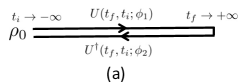
Figure 1: Closed time path contour in a state given by density matrix $\rho_{0}$. The two lines represent path integrals along two copies of spacetime with arrows indicating the direction of integrations. (a) and (b) correspond to having $\rho_{0}$ as the initial and final state respectively.

Here we discuss the motivations behind the $Z_{2}$ symmetry (12), and some simple examples.

Now consider CTP generating functional (2) with $\rho_{0}$ given by an initial thermal density matrix with inverse temperature $\beta_{0}$ (see Fig. 1(a)). Alternatively we can also consider the generating functional $W_{T}$ defined by Fig. 1(b) with density matrix $\rho_{0}$ imposed at $t=+\infty$ rather than at $t=-\infty$, i.e.

$$e^{W_{T}[\phi_{1i},\phi_{2i}]} =\mathop{\rm Tr}\left[U^{\dagger}(+\infty,-\infty;\phi_{2i})\rho_{0}U(+\infty,-\infty;\phi_{1i})\right]\ .$$ (70)

For a system with ${{\mathcal{P}}}{\mathcal{T}}$ symmetry then we have

$$W[\phi_{1i},\phi_{2i}]=W_{T}[\phi_{1i}^{PT},\phi_{2i}^{PT}],\qquad\phi_{i}^{PT}(x)\equiv\eta_{i}^{PT}\phi_{i}(-x)\$$ (71)

where $x$ denotes $x^{\mu}=(x^{0},x^{i})=(t,{\vec{x}})$. $W$ and $W_{T}$ are also related by the Kubo-Martin-Schwinger (KMS) condition kubo57 ; mart59 ; Kadanoff

$${W[\phi_{1i},\phi_{2i}]}=W_{T}[\phi_{1i}(t+i{\theta}),\phi_{2i}(t-i(\beta_{0}-{\theta}))]$$ (72)

for ${\theta}\in[0,\beta_{0}]$ (see Sec. IIC of CGL for more details). From (71) and (72) we thus find that

$$W[\phi_{1}(x),\phi_{2}(x)]=W[\tilde{\phi}_{1}(x);\tilde{\phi}_{2}(x)]$$ (73)

with

$$\begin{split}\tilde{\phi}_{1}(x)=\phi_{1}(-t+i{\theta},-{\vec{x}}),\qquad\tilde{\phi}_{2}(x)=\phi_{2}(-t-i(\beta_{0}-{\theta}),-{\vec{x}})\ \end{split}$$ (74)

where for simplicity we have taken $\eta^{PT}=1$. For a theory whose dynamical variables $\chi$ are non-conserved quantities, the couplings between dynamical variables $\chi$ and the sources $\phi$ can be written in a linear form

$$I_{\rm EFT}[\chi_{1},\phi_{1};\chi_{2},\phi_{2}]=\cdots+\int d^{d}x\,\left(\chi_{1}\phi_{1}-\chi_{2}\phi_{2}\right)\ .$$ (75)

It can be readily checked that (73) is satisfied if we require that $I_{\rm EFT}$ satisfy

$$I_{\rm EFT}[\chi_{1},\phi_{1};\chi_{2},\phi_{2}]=I_{\rm EFT}[\tilde{\chi}_{1},\tilde{\phi}_{1};\tilde{\chi}_{2},\tilde{\phi}_{2}]$$ (76)

where $\tilde{\phi}_{1,2}$ are given by (74) and

$$\begin{split}\tilde{\chi}_{1}(x)=\chi_{1}(-t+i{\theta},-{\vec{x}}),\qquad\tilde{\chi}_{2}(x)=\chi_{2}(-t-i(\beta_{0}-{\theta}),-{\vec{x}})\ .\end{split}$$ (77)

In the classical $\hbar\to 0$ limit $\phi_{a},\chi_{a}\to\hbar(\phi_{a},\chi_{a})$ and $\phi_{r},\chi_{r}\to\phi_{r},\chi_{r}$. Restoring the $\hbar$ in $\beta_{0}\hbar,{\theta}\hbar$ in (74) and (77) we then find (74) and (77) become

$$\tilde{\phi}_{r}(x)=\phi_{r}(-x),\qquad\tilde{\phi}_{a}(x)=\phi_{a}(-x)+i\beta_{0}\partial_{0}\phi_{r}(-x)$$ (78)

$$\tilde{\chi}_{r}(x)=\chi_{r}(-x),\qquad\tilde{\chi}_{a}(x)=\chi_{a}(-x)+i\beta_{0}\partial_{0}\chi_{r}(-x)\ .$$ (79)

Transformations for $\chi_{r{\rm i}},\chi_{a{\rm i}}$ in (13) are generalization of (79) to local equilibrium. The transformations (13) for hydrodynamical variables are discussed in detail in CGL1 .

Similarly from (71) and (72) we find for $W_{T}$ that

$$W_{T}[\phi_{1},\phi_{2}]=W[\phi_{1}^{PT},\phi_{2}^{PT}]=W_{T}[\phi_{1}(-t-i{\theta},-{\vec{x}}),\phi_{2}(-t+i(\beta_{0}-{\theta}),-{\vec{x}})]\$$ (80)

and equations (78) become

$$\tilde{\phi}_{r}(x)=\phi_{r}(-x),\qquad\tilde{\phi}_{a}(x)=\phi_{a}(-x)-i\beta_{0}\partial_{0}\phi_{r}(-x)\\$$ (81)

i.e. with a minus sign in the second second in the transformation of $\phi_{a}$. Accordingly the dynamical KMS transformation (79) should be replaced by

$$\tilde{\chi}_{r}(-x)=\chi_{r}(x),\qquad\tilde{\chi}_{a}(-x)=\chi_{a}(x)-i\beta_{0}\partial_{0}\chi_{r}(x)\ .$$ (82)

We thus conclude that the sign in transformation of $\Phi_{a}$ in (13) may be considered as for a local equilibrium established in the past, the sign in (54) may be considered as for a local equilibrium established in the future.

Appendix C Imposing the dynamical KMS condition

Here we elaborate a bit further on imposing the dynamical KMS conditions (21) and (22). We first note that there is a simple trick to impose conditions (22) with $k\geq 1$, which also makes manifest that one can set $V_{k}^{\mu}$ to zero by absorbing them into the definition of the Lagrangian. Consider a Lagrangian density ${{\mathcal{L}}}_{0}$ of the form (8). Due to $Z_{2}$ nature of the transformation,

$${{\mathcal{L}}}={{\frac{1}{2}}}\left({{\mathcal{L}}}_{0}+\tilde{{\mathcal{L}}}_{0}\right),$$ (83)

where $\tilde{{\mathcal{L}}}_{0}$ is obtained from ${{\mathcal{L}}}_{0}$ by acting transformations (13), automatically satisfies (22) without the need for any total derivatives. Note, however, that $\tilde{{\mathcal{L}}}_{0}$ in general contains terms with $r$-fields only, and we must then further require that such terms in $\tilde{{\mathcal{L}}}_{0}$ vanish, which is precisely (21).

For $k=1$ we will need to perform a further integration by parts to write $f^{(1)}$ terms in the Lagrangian in the form of (10), with no further derivatives on $a$-variables. This can generate a nonzero $V_{1}^{\mu}$. We now show that $\partial_{\mu}V_{1}^{\mu}$ contains only odd number of derivatives. Acting dynamical KMS transformation on both sides of (18) we have

$$\mathcal{L}-\tilde{\mathcal{L}}=-\partial_{\mu}\tilde{V}^{\mu},$$ (84)

where we used that the dynamical KMS transformation is $Z_{2}$, and that $\tilde{V}^{\mu}$ denotes the dynamical KMS transformed of $V^{\mu}$. Comparing (84) with (18) we find that $\tilde{V}^{\mu}=V^{\mu}$. Now given that $V^{\mu}=V_{0}^{\mu}+V_{1}^{\mu}$, we then conclude that $V_{1}^{\mu}$ can only contain even number of derivatives.

Appendix D Examples

Here we discuss some two explicit examples.

D.1 Model A

As an illustration of a system with no conservation laws, we consider the critical dynamics of a $n$-component real order parameter $\chi_{\rm i},{\rm i}=1,\cdots,n$ (i.e. model A hohenberg ; Folk ). We will ignore couplings to hydrodynamic modes, i.e. the system is at a fixed inverse temperature $\beta_{0}$ and $\beta^{\mu}=(\beta_{0},\vec{0})$. In (8) $\Lambda_{r}$ and $\Phi_{a}$ are then $\chi_{r{\rm i}}$ and $\chi_{a{\rm i}}$ respectively, and the dynamical KMS transformations (13) become

$$\tilde{\chi}_{r{\rm i}}(x)=\chi_{r{\rm i}}(-x),\qquad\tilde{\chi}_{a{\rm i}}(-x)=\chi_{a{\rm i}}(x)+{i\beta_{0}}\partial_{0}\chi_{r{\rm i}}(x)\ .$$ (85)

As (85) only involves time derivative we can treat time and spatial derivatives separately. For simplicity we consider the first two terms in (8) which can be written explicitly as

$${{\mathcal{L}}}=E^{\rm i}\chi_{a{\rm i}}+iX^{{\rm i}{\rm j}}\chi_{a{\rm i}}\chi_{a{\rm j}}+\cdots\$$ (86)

where one should keep in mind that $X^{{\rm i}{\rm j}}$ may include derivatives on $\chi_{a}$’s and thus do not have to be symmetric in exchanging ${\rm i},{\rm j}$ indices. We can expand $E$ and $X$ in the number of time derivatives as

$$E^{\rm i}=E_{0}^{\rm i}+E^{\rm i}_{1}+\cdots,\qquad X^{{\rm i}{\rm j}}=X^{{\rm i}{\rm j}}_{0}+X^{{\rm i}{\rm j}}_{1}+\cdots$$ (87)

and each term can be further expanded in terms of the number of spatial derivatives.

Applying (83) to (86) we can read the consequences of (22)

$$E_{1}^{\rm i}=-{{\frac{1}{2}}}(X^{{\rm i}{\rm j}}_{0}+X^{{\rm j}{\rm i}}_{0})\Phi_{{\rm j}},\quad\Phi_{\rm i}\equiv\beta_{0}\partial_{0}\chi_{r{\rm i}}\ .$$ (88)

Now for simplicity let us further restrict to zero spatial derivative in $X_{0}$, i.e.

$$X_{0}^{{\rm i}{\rm j}}=f^{{\rm i}{\rm j}}(\chi_{r})\quad\Rightarrow\quad E_{1}^{\rm i}=-f^{{\rm i}{\rm j}}(\chi_{r})\Phi_{{\rm j}}\ .$$ (89)

$f^{{\rm i}{\rm j}}$ is symmetric in its indices, which leads to the Onsager relations. Applying (21) to (86), we find

$$E^{\rm i}_{0}\Phi_{\rm i}=\partial_{\mu}V^{\mu}_{(0,0)},\qquad-E^{{\rm i}}_{1}\Phi_{\rm i}-X^{{\rm i}{\rm j}}_{0}\Phi_{\rm i}\Phi_{\rm j}=\partial_{\mu}V^{\mu}_{(0,1)}$$ (90)

where $V^{\mu}_{(0,n)}$ contains $n$ time derivatives. The second equation is automatically satisfied with $V^{\mu}_{(0,1)}=0$ due to (89). The first equation can be solved to all orders in spatial derivatives if there exists a local functional ${{\mathcal{F}}}(t;\chi_{r}]$ (in (91) there are only spatial integrations)

$${{\mathcal{F}}}(t;\chi_{r}]=\int d^{d-1}\vec{x}\,F(\chi_{r}(x),\partial_{i}\chi_{r}(x),\cdots)$$ (91)

from which

$$E_{0}^{\rm i}=-{{{\delta}}{{\mathcal{F}}}\over{{\delta}}\chi_{r{\rm i}}(x)}=-{\partial F\over\partial\chi_{r{\rm i}}}+\partial_{i}\left({\partial F\over\partial\partial_{i}\chi_{r{\rm i}}}\right)-\partial_{i}^{2}\left({\partial F\over\partial\partial_{i}^{2}\chi_{r{\rm i}}}\right)+\cdots$$ (92)

and accordingly

$$V^{0}_{(0,0)}=-\beta_{0}F,\qquad{1\over\beta_{0}}V^{i}_{(0,0)}={\partial F\over\partial\partial_{i}\chi_{r{\rm i}}}\partial_{0}\chi_{r{\rm i}}+{\partial F\over\partial\partial_{i}^{2}\chi_{r{\rm i}}}\partial_{i}\partial_{0}\chi_{r{\rm i}}-\partial_{i}{\partial F\over\partial\partial_{i}^{2}\chi_{r{\rm i}}}\partial_{0}\chi_{r{\rm i}}+\cdots\ .$$ (93)

Collecting various expressions above, we can write the Lagrangian as

$${{\mathcal{L}}}_{\rm eff}=\left(-{{{\delta}}{{\mathcal{F}}}\over{{\delta}}\chi_{r{\rm i}}}-\beta_{0}f^{{\rm i}{\rm j}}\partial_{0}\chi_{r{\rm j}}\right)\chi_{a{\rm i}}+{i}f^{{\rm i}{\rm j}}(\chi_{r})\chi_{a{\rm i}}\chi_{a{\rm j}}+\cdots\ .$$ (94)

Equation (6) also requires that for arbitrary $a_{\rm i}(x)$

$$f^{{\rm i}{\rm j}}(\chi_{r})a_{\rm i}(x)a_{\rm j}(x)\geq 0\ .$$ (95)

We can now readily write the entropy current to the order exhibited in (94) by applying equation (28), which gives

$$S^{\mu}=V^{\mu}_{0}\ .$$ (96)

More explicitly,

$$S^{0}=-\beta_{0}F,\qquad S^{i}=\beta_{0}\left({\partial F\over\partial\partial_{i}\chi_{r{\rm i}}}\partial_{0}\chi_{r{\rm i}}+{\partial F\over\partial\partial_{i}^{2}\chi_{r{\rm i}}}\partial_{i}\partial_{0}\chi_{r{\rm i}}-\partial_{i}{\partial F\over\partial\partial_{i}^{2}\chi_{r{\rm i}}}\partial_{0}\chi_{r{\rm i}}+\cdots\right)$$ (97)

and one can readily check after using equations of motion

$$\partial_{\mu}S^{\mu}=\beta_{0}^{2}f_{{\rm i}{\rm j}}\partial_{0}\chi_{r{\rm j}}\partial_{0}\chi_{r{\rm i}}\geq 0\ .$$ (98)

At zeroth order in time derivatives we have

$$S_{0}^{0}=-\beta_{0}F,\qquad S^{i}_{0}=0\$$ (99)

which has the standard form with $F$ interpreted as the (static) free energy density of the scalar system.

Let us now consider a phase whose equilibrium configuration has $\chi_{r{\rm i}}=0$ and $\chi_{r{\rm i}},\chi_{a{\rm i}}$ are small. Keeping only quadratic terms in (94), we can write

$$f^{{\rm i}{\rm j}}={1\over{{\Gamma}}_{0}}{{\delta}}^{{\rm i}{\rm j}},\qquad F={{\frac{1}{2}}}r\chi_{r{\rm i}}^{2}+{{\frac{1}{2}}}(\partial_{i}\chi_{{\rm i}})^{2}+\cdots$$ (100)

where we have only kept two spatial derivatives in $F$. ${{\Gamma}}_{0}$ should be non-negative due to (95). $F$ (and thus the constant $r$) should also be non-negative to ensure thermodynamic stability. With an external source $\phi_{r}$, the quadratic Lagrangian can be written as

$${{\mathcal{L}}}=\left(-r\chi_{r{\rm i}}+\partial_{i}^{2}\chi_{r{\rm i}}-{\beta_{0}\over{{\Gamma}}_{0}}\partial_{0}\chi_{r{\rm j}}\right)\chi_{a{\rm i}}+{i\over{{\Gamma}}_{0}}\chi_{a{\rm i}}\chi_{a{\rm i}}+\phi_{r{\rm i}}\chi_{a{\rm i}}\$$ (101)

and the equations of motion for $\chi_{r{\rm i}}$ are

$${{\gamma}}_{0}\partial_{0}\chi_{r{\rm i}}+r\chi_{r{\rm i}}-\partial_{i}^{2}\chi_{r{\rm i}}=\phi_{r{\rm i}}\$$ (102)

where the “friction” coefficient

$${{\gamma}}_{0}=\beta_{0}{{\Gamma}}_{0}\$$ (103)

is also non-negative, i.e. $\chi_{r{\rm i}}$ will be damped. Equivalently we find the response function in momentum space

$$\chi_{r{\rm i}}(\omega,{\vec{k}})={\phi_{r{\rm i}}(\omega,{\vec{k}})\over-i{{\gamma}}_{0}\omega+r+k^{2}}$$ (104)

has a pole in the lower half complex $\omega$-plane.

Now consider changing the sign of the second term in (85), which may be considered as taking $\beta_{0}\to-\beta_{0}$ we then find that the new current which we denotes as $\hat{S}^{\mu}$ has opposite signs to (97), but still satisfies

$$\partial_{\mu}\hat{S}^{\mu}=\beta_{0}^{2}f_{{\rm i}{\rm j}}\partial_{0}\chi_{r{\rm j}}\partial_{0}\chi_{r{\rm i}}\geq 0\ .$$ (105)

To match with the standard equilibrium expression for the entropy density, we then need to identify the new entropy current $S^{\mu}_{T}$ as $-\hat{S}^{\mu}$, which then satisfies

$$\partial_{\mu}S^{\mu}_{T}=-\beta_{0}^{2}f_{{\rm i}{\rm j}}\partial_{0}\chi_{r{\rm j}}\partial_{0}\chi_{r{\rm i}}\leq 0\ .$$ (106)

In (103), ${{\gamma}}_{0}$ also changes sign and now the pole of (104) lies in the upper half plane. Thus both thermodynamic and causal arrows of time switch.

D.2 Fluctuating hydrodynamics for relativistic charged fluids

We now briefly outline the story for fluctuating hydrodynamics of a relativistic charged fluids in the classical limit. More details can be found CGL1 .

The dynamical variables are then hydrodynamical modes associated with conserved quantities. The $r$-variables $\beta^{\mu}=\beta(x)u^{\mu}(x)$ and ${\hat{\mu}}=\beta(x)\mu(x)$ can be written in a uniform manner as $\beta_{M}=(\beta_{\mu},\hat{\mu})$. The $a$-variables can be written in a uniform manner as $X_{aM}=(X_{a\mu},\varphi_{a})$. Equation (13) can also be written uniformly as

$$\partial_{\mu}\tilde{X}_{aM}(-x)=\partial_{\mu}\tilde{X}_{aM}(x)+i\partial_{\mu}\beta_{M}(x)$$ (107)

and the first two terms of (8) can be written more explicitly as

$${{\mathcal{L}}}_{\rm eff}=T^{\mu M}\partial_{\mu}X_{aM}+iW^{\mu\nu,MN}\partial_{\mu}X_{aM}\partial_{\nu}X_{aN}+\cdots\ .$$ (108)

with $T^{\mu M}=(T^{\mu\nu},J^{\nu})$ the hydrodynamic stress tensor and $U(1)$ current. We will consider (108) to one derivatives in $T^{\mu M}$ and zero derivative in $W^{\mu\nu,MN}$.

Applying (83) we find

$$T^{\mu M}_{1}=-W^{\mu\nu,MN}_{0}\partial_{\nu}\beta_{N}$$ (109)

and equation (21) requires

$$T^{\mu M}_{0}\partial_{\mu}\beta_{M}=\partial_{\mu}V^{\mu}_{(0,0)},\quad T^{\mu M}_{1}\partial_{\mu}\beta_{M}+W^{\mu\nu,MN}_{0}\partial_{\mu}\beta_{M}\partial_{\nu}\beta_{N}=\partial_{\mu}V^{\mu}_{(0,1)}$$ (110)

where subscripts in $T$ and $W$ now denote the total number of derivatives and so does the second subscript of $V^{\mu}$. Note from (109) the second equation of (110) is automatically satisfied with $V^{\mu}_{(0,1)}=0$.

At zeroth derivative order, we can write $T^{\mu M}_{0}=(T_{0}^{\mu\nu},J^{\mu}_{0})$ as

$$T_{0}^{\mu\nu}=\varepsilon_{0}u^{\mu}u^{\nu}+p_{0}\Delta^{\mu\nu},\quad J^{\mu}_{0}=n_{0}u^{\mu}\$$ (111)

where $\epsilon_{0},p_{0},n_{0}$ are functions of $\beta$ and ${\hat{\mu}}$. The first equation of (110) then requires $\epsilon_{0},p_{0},n_{0}$ satisfy the standard thermodynamic relations

$$\epsilon_{0}+p_{0}=-\beta{\partial p_{0}\over\partial\beta},\qquad n_{0}=\beta{\partial p_{0}\over\partial{\hat{\mu}}},$$ (112)

with

$$V_{(0,0)}^{\mu}=p_{0}\beta^{\mu}\ .$$ (113)

In other words, the first law of thermodynamics is satisfied locally. Equation (109) ensures that $T^{\mu M}$ satisfies the Onsager relations due to $W^{\mu\nu,MN}_{0}=W^{\nu\mu,NM}_{0}$.

From (28) the entropy current to first derivative order can be written as

$$S^{\mu}=p_{0}\beta^{\mu}-T^{\mu\nu}\beta_{\mu}-J^{\mu}{\hat{\mu}}\$$ (114)

and one can readily check that by using equations of motion

$$\partial_{\mu}S^{\mu}=W_{0}^{\mu\nu,MN}\nabla_{\mu}\beta_{M}\nabla_{\nu}\beta_{N}\geq 0\ .$$ (115)

With a bit more effort the right hand side of the above equation can be expressed in a conventional form using conductivity, shear viscosity and bulk viscosity, see CGL1 , where we also generalize the above entropy current analysis to second order in derivative expansion.

Linear responses from the effective action (108) have been discussed in details in CGL . Here we only mention some key elements. The response functions have poles only in the lower half $\omega$-plane provided that the leading dissipative coefficients, which are conductivity $\sigma$, shear viscosity $\eta$, and bulk viscosity $\kappa$, are all non-negative. These dissipative coefficients are indeed non-negative as they can be expressed via (109) schematically as

$$\sigma=\beta A_{1},\qquad\eta=\beta A_{2},\qquad\kappa=\beta A_{3}$$ (116)

where $A_{1,2,3}$ are combinations coefficients of $W_{0}$ and are non-negative separately from (6).

Now let us consider reverse the sign in (107), which can be achieved by taking $\beta\to-\beta$ in various places. The resulting $\hat{S}^{\mu}_{0}$ has an opposite overall sign to (114) and satisfy $\partial_{\mu}\hat{S}^{\mu}\geq 0$. Matching with the standard thermodynamic entropy we should identify $S_{T}^{\mu}=-\hat{S}^{\mu}$, which then has a negative divergence. Similarly all the dissipative coefficients in (116) change signs and now the poles of response functions lie in upper half frequency plane.

Appendix E Details of proof

In this Appendix we provide details for the manipulations from (32) to (36). First we verify that (34)–(35) solve (32)–(33). Plugging (34) into (32) and rearranging the double sum of the second term on left hand side we find that

$${1\over 2m+1}\sum_{k=0}^{l}(-1)^{k}C_{2m+2k+2}^{2m}G_{2k+2}F^{(2m+2k+2,2l-2k)}$$ (117)

$${{\frac{1}{2}}}{1\over 2m+1}\sum_{k=1}^{l}(-1)^{k}C_{2m+2k+2}^{2m}F^{(2m+2k+2,2l-2k)}\left(\sum_{n=1}^{k}C_{2k+2}^{2n}G_{2n}\right)$$ (118)

$$={{\frac{1}{2}}}\sum_{k=0}^{l}(-1)^{k+1}C_{2m+2k+2}^{2k+1}F^{(2m+2k+2,2l-2k)}\ .$$ (119)

$k=0$ term in the above equation is satisfied as $G_{2}=-1$. The terms with $1\leq k\leq l$ are satisfied from the identities (equation (137) of Appendix E.1)

$$-G_{2k+2}-{1\over 2}\left(\sum_{n=1}^{k}C_{2k+2}^{2n}G_{2n}\right)=k+1,\qquad k=1,2,\cdots\ .$$ (120)

Similarly plugging (35) into (33) and rearranging the double sum on the left hand side we find

$${2\over 2m-1}\sum_{k=0}^{l}(-1)^{k}C_{2m+2k}^{2m-2}F^{(2m+2k,2l-2k+1)}\left(\sum_{n=0}^{k}C_{2k+2}^{2n}B_{2n}\right)=\sum_{k=0}^{l}(-1)^{k}C_{2m+2k}^{2m-1}F^{(2m+2k,2l-2k+1)}$$ (121)

which are indeed satisfied given the identities (equation (136) of Appendix E.1)

$${1\over k+1}\sum_{n=0}^{k}C_{2k+2}^{2n}B_{2n}=1,\qquad k=0,1,\cdots\ .$$ (122)

Now let us give intermediate steps leading to (36). Plugging (34)–(35) into (31), we find for $n\geq 1$

$$\partial_{\mu}S_{2n-1}^{\mu}=F^{(2,2n-2)}+\sum_{k=2}^{n}o_{k}F^{(2k,2n-2k)},\qquad\partial_{\mu}S_{2n}^{\mu}=\sum_{k=1}^{n}e_{k}F^{(2k,2n-2k+1)}$$ (123)

with

$$o_{k}=(-1)^{k+1}\left(1+{1\over 2k+1}\sum_{l=1}^{k-1}C_{2k+1}^{2l}G_{2l}\right),\quad e_{k}=(-1)^{k+1}\left(1-{2\over 2k+1}\sum_{l=0}^{k-1}C_{2k+1}^{2l}B_{2l}\right)\ .$$ (124)

Using the identities (138) and (135) of Appendix E.1 we find

$$o_{k}=(-1)^{k}G_{2k},\qquad e_{k}=2(-1)^{k+1}B_{2k}$$ (125)

which then give (36).

To conclude this subsection let us elucidate the structure of equations (32)–(33) which can be rewritten as two infinite families of upper triangular linear equations. More explicitly, for each integer $l\geq 1$, introducing column vectors

$$A^{(l)}=\left(\begin{matrix}F^{(3,2l-1)}\cr\vdots\cr F^{(2l+1,1)}\end{matrix}\right),\quad B^{(l)}=\left(\begin{matrix}F^{(4,2l-2)}\cr\vdots\cr F^{(2l+2,0)}\end{matrix}\right),\quad C^{(l)}=\left(\begin{matrix}F^{(3,2l-2)}\cr\vdots\cr F^{(2l+1,0)}\end{matrix}\right),\quad D^{(l)}=\left(\begin{matrix}F^{(2,2l-1)}\cr\vdots\cr F^{(2l,1)}\end{matrix}\right),$$ (126)

i.e. for $m=1,\cdots,l$

$$A_{m}^{(l)}=F^{(2m+1,2l-2m+1)},\quad B_{m}^{(l)}=F^{(2m+2,2l-2m)},\quad C_{m}^{(l)}=F^{(2m+1,2l-2m)},\quad D_{m}^{(l)}=F^{(2m,2l-2m+1)},$$ (127)

then we can write (32)–(33) as

$$K^{(l)}\cdot A^{(l)}=L^{(l)}\cdot B^{(l)},\qquad M^{(l)}\cdot C^{(l)}=N^{(l)}\cdot D^{(l)}$$ (128)

where $K^{(l)},L^{(l)},M^{(l)},N^{(l)}$ are $l\times l$ upper triangular matrices. Their non-vanishing matrix elements are given by

$$K^{(l)}_{m,m+k}={{\delta}}_{k,0}+{{\frac{1}{2}}}(-1)^{k}C_{2m+1+2k}^{2m+1},\quad L^{(l)}_{m,m+k}={{\frac{1}{2}}}(-1)^{k+1}C_{2m+2k+2}^{2m+1},$$ (129)

$$M^{(l)}_{m,m+k}=(-1)^{k+1}C_{2m+2k+1}^{2m-1},\quad N^{(l)}_{m,m+k}=(-1)^{k+1}C_{2m+2k}^{2m-1}$$ (130)

where $m=1,2,\cdots,l$ and $k=0,1,\cdots l-m$. The solution (34)–(35) implies the identities

$$(K^{(l)})^{-1}L^{(l)}=P^{(l)},\qquad(M^{(l)})^{-1}N^{(l)}=Q^{(l)}$$ (131)

where $P^{(l)},Q^{(l)}$ are upper triangular matrices with nonzero entries given by

$$P^{(l)}_{m,m+k}={(-1)^{k}\over 2m+1}C_{2m+2k+2}^{2m}G_{2k+2},\qquad Q^{(l)}_{m,m+k}={2(-1)^{k}\over 2m+1}C_{2m+2k}^{2k}B_{2k}$$ (132)

for $m=1,2,\cdots,l$ and $k=0,1,\cdots l-m$.

E.1 Bernoulli and Genocchi numbers

Here we collect some facts and identities regarding Bernoulli and Genocchi numbers. Firstly note the following recursion relations for Bernouli and numbers bernouli ; genocchi

$$B_{m}=1-\sum_{k=0}^{m-1}C_{m}^{k}{B_{k}\over m-k+1}=1-{1\over m+1}\sum_{k=0}^{m-1}C_{m+1}^{k}B_{k},\quad m\geq 1\quad{\rm with}\;B_{1}={{\frac{1}{2}}},$$ (133)

$$2G_{m}+\sum_{k=1}^{m-1}C_{m}^{k}G_{k}=0,\quad m\geq 2,\quad{\rm with}\;\;G_{1}=1\ .$$ (134)

Taking $m=2k$ and $m=2k+1$ respectively in (133) we have

$$B_{2k}={{\frac{1}{2}}}-{1\over 2k+1}\sum_{l=0}^{k-1}C_{2k+1}^{2l}B_{2l},\quad k=1,2,\cdots$$ (135)

$$0={{\frac{1}{2}}}-{1\over 2k}\sum_{l=0}^{k-1}C_{2k}^{2l}B_{2l},\quad k=1,2,\cdots\ .$$ (136)

Similarly taking $m=2k$ and $m=2k+1$ respectively in (134) we find

$$G_{2k}+k+{{\frac{1}{2}}}\sum_{l=1}^{k-1}C_{2k}^{2l}G_{2l}=0,\quad k=1,2,\cdots$$ (137)

$$\sum_{l=1}^{2k}C_{2k+1}^{l}G_{l}=0\quad\to\quad G_{2k}+1+{1\over 2k+1}\sum_{l=1}^{k-1}C_{2k+1}^{2l}G_{2l}=0,\quad k=1,2,\cdots\ .$$ (138)

E.2 Two identities

Consider the function

$$f(x)=\sum_{k=1}^{\infty}c_{2k}x^{2k},$$ (139)

such that $f(x)$ goes to zero sufficiently fast as $x\to\pm\infty$. Then

$$\sum_{k=1}^{\infty}(-1)^{k}G_{2k}c_{2k}=\pi\int_{-\infty}^{\infty}\frac{\cosh(\pi x)}{\sinh^{2}(\pi x)}f(x)dx,$$ (140)

$$2\sum_{k=1}^{\infty}(-1)^{k+1}B_{2k}c_{2k}=\pi\int_{-\infty}^{\infty}\frac{1}{\sinh^{2}(\pi x)}f(x)dx$$ (141)

which follow from the integral representations of the Bernoulli numbers wolfram

$$2(-1)^{k+1}B_{2k}=\pi\int_{-\infty}^{\infty}dx\,\frac{1}{\sinh^{2}(\pi x)}x^{2k},\quad(-1)^{k}G_{2k}=\pi\int_{-\infty}^{\infty}dx\,\frac{\cosh(\pi x)}{\sinh^{2}(\pi x)}x^{2k}\ .$$ (142)

Appendix F Non-negativity of zeroth order Lagrangian

Consider an action

$$S=\int d^{d}x\,{{\mathcal{L}}}\left(\phi(x),\partial_{\mu}\phi(x),\cdots\right)\ .$$ (143)

Now suppose we have

$$S\geq 0$$ (144)

for any choice of $\phi(x)$. We would like to show that

$${{\mathcal{L}}}_{0}\geq 0$$ (145)

for any $\phi$, where ${{\mathcal{L}}}_{0}$ denote the zero derivative part of ${{\mathcal{L}}}$.

Take $\phi(x)=\phi_{0}$ where $\phi_{0}$ is any constant, then we have

$$S=V{{\mathcal{L}}}_{0}(\phi_{0})\geq 0\quad\to\quad{{\mathcal{L}}}_{0}(\phi_{0})\geq 0$$ (146)

where $V$ here denotes the spacetime volume. We thus find

$${{\mathcal{L}}}_{0}(\phi(x))\geq 0$$ (147)

for any $x$.

One can also readily see from $S\geq 0$ one cannot conclude the full Lagrangian density to be non-negative. Consider adding to ${{\mathcal{L}}}$ a total derivative

$${{\mathcal{L}}}^{\prime}={{\mathcal{L}}}+\partial_{\mu}V^{\mu}\ .$$ (148)

$S$ does not change, but at a given point $x$ it appears that no matter what the value of ${{\mathcal{L}}}$ is we can always arrange $V^{\mu}$ to make ${{\mathcal{L}}}^{\prime}$ to be negative. Note that adding a total derivative does not change ${{\mathcal{L}}}_{0}$.

One could contemplate whether it is possible to use the freedom of adding total derivatives to choose to a Lagrangian ${{\mathcal{L}}}\geq 0$. It is not clear to us whether this is possible or not.

References

- (1) L. D. Landau and E. M. Lifshitz, “Fluid Mechanics,” Pergamon Press, Oxford (1987).
- (2) H. Janssen, Z. Phys. B23, 377 (1976).
- (3) R. Bausch, H. K. Janssen, and H. Wagner, Z. Phys. B24, 113 (1976).
- (4) L. M. Sieberer, A. Chiocchetta, A. Gambassi, U. C. Tauber, and S. Diehl, Phys. Rev. B 92 134307 (2015); arXiv:1505.00912.
- (5) M. Crossley, P. Glorioso and H. Liu, “Effective field theory of dissipative fluids,” arXiv:1511.03646 [hep-th].
- (6) P. Glorioso, M. Crossley, and H. Liu, “Effective field theory for dissipative fluids (II): classical limit, dynamical KMS symmetry and entropy current,” arXiv:1701.07817 [hep-th].
- (7) L. Boltzmann, “Lectures on Gas Theory,” Dover Publishing Co., New York (1995).
- (8) G. N. Bochkov and Y. E. Kuzovlev, Sov. Phys. JETP 45, 125 (1977).
- (9) C. Jarzynski, Phys. Rev. Lett. 78, 2690 (1997).
- (10) G. E. Crooks, Phys. Rev. E 60, 2721 (1999).
- (11) N. Banerjee, J. Bhattacharya, S. Bhattacharyya, S. Jain, S. Minwalla and T. Sharma, JHEP 1209, 046 (2012) [arXiv:1203.3544 [hep-th]].
- (12) K. Jensen, M. Kaminski, P. Kovtun, R. Meyer, A. Ritz and A. Yarom, Phys. Rev. Lett. 109, 101601 (2012) [arXiv:1203.3556 [hep-th]].
- (13) S. Bhattacharyya, JHEP 1408, 165 (2014) [arXiv:1312.0220 [hep-th]].
- (14) S. Bhattacharyya, JHEP 1407, 139 (2014) [arXiv:1403.7639 [hep-th]].
- (15) S. Dubovsky, T. Gregoire, A. Nicolis and R. Rattazzi, JHEP 0603, 025 (2006) [hep-th/0512260].
- (16) S. Dubovsky, L. Hui, A. Nicolis and D. T. Son, Phys. Rev. D 85, 085029 (2012) [arXiv:1107.0731 [hep-th]].
- (17) J. de Boer, M. P. Heller and N. Pinzani-Fokeeva, JHEP 1508, 086 (2015) [arXiv:1504.07616 [hep-th]].
- (18) F. M. Haehl, R. Loganayagam and M. Rangamani, Phys. Rev. Lett. 114, 201601 (2015) [arXiv:1412.1090 [hep-th]]. F. M. Haehl, R. Loganayagam and M. Rangamani, JHEP 1505, 060 (2015) [arXiv:1502.00636 [hep-th]].
- (19) F. M. Haehl, R. Loganayagam and M. Rangamani, JHEP 1604, 039 (2016) [arXiv:1511.07809 [hep-th]].
- (20) J. Schwinger, J. Math. Phys. 2, 407 (1961); Particles and Sources, vol. I., II., and III., Addison-Wesley, Cambridge, Mass. 1970-73.
- (21) L. V. Keldysh, Zh. Eksp. Teor. Fiz. 47, 1515 (1964) (Sov. Phys. JETP 20, 1018 (1965)).
- (22) R. P. Feynman and F. L. Vernon, Jr., Annals Phys. 24, 118 (1963) [Annals Phys. 281, 547 (2000)].
- (23) K. C. Chou, Z. B. Su, B. L. Hao and L. Yu, Phys. Rept. 118, 1 (1985).
- (24) S. Grozdanov and J. Polonyi, arXiv:1305.3670 [hep-th].
- (25) M. Harder, P. Kovtun and A. Ritz, JHEP 1507, 025 (2015) [arXiv:1502.03076 [hep-th]].
- (26) P. Kovtun, G. D. Moore and P. Romatschke, JHEP 1407 (2014) 123 [arXiv:1405.3967 [hep-ph]].
- (27) N. N. Bogoliubov, J. Phys. U.S.S.R. 10, 265 (1946).
- (28) E. G. D. Cohen and T. H. Berlin, Physica 26 717 (1960).
- (29) T.-Y. Wu, Int. J. Theor. Phys. 2, 325 (1969).
- (30) M. Campisi and P. Hänggi, Entropy, 13 2024 (2011).
- (31) C. Jarzynski, Ann. Rev. Condens. Matter. Phys. 2, 329 (2011).
- (32) D. J. Evans and D. J. Searles, Phys. Rev. E53, 5808 (1996).
- (33) M. Campisi, P. Hänggi and P. Talkner, Rev. Mod. Phys., 83 771 (2011).
- (34) R. Kubo, J. Math. Soc. Japan 12 570 (1957).
- (35) P. C. Martin and J. Schwinger, Phys. Rev. 115 1342 (1959).
- (36) L. P. Kadanoff and P. C. Martin, Ann. Phys. 24, 419 (1963).
- (37) P. C. Hohenberg and B. I. Halperin, Rev. Mod. Phys. 49, 435 (1977).
- (38) R. Folk and G. Moser, J. Phys. A39, R207 (2006).
- (39) Wikipedia page on Bernouli numbers
- (40) C.-H. Chang and C.-W. Ha, Bull. Austral. Math. Soc. 64 469 (2001).
- (41) The Wolfram Functions Site, http://functions.wolfram.com/IntegerFunctions/BernoulliB/07/