Minimal non-universal EW extensions of the Standard Model: a chiral multi-parameter solution

Abstract

We report the most general expression for the chiral charges of a non-universal $U(1)^{\prime}$ with identical charges for the first two families but different charges for the third one. The model is minimal in the sense that only standard model fermions plus right-handed neutrinos are required. By imposing anomaly cancellation and constraints coming from Yukawa couplings we obtain two different solutions. In one of these solutions, the anomalies cancel between fermions in different families. These solutions depend on four independent parameters which result very useful for model building. We build different benchmark models in order to show the flexibility of the parameterization. We also report LHC and low energy constraints for these benchmark models.

1 Introduction

In the present work we address the question: what is the minimal electroweak extension of the standard model (SM) with a minimal content of fermions? By itself, this question is interesting and deserves a dedicated and systematic study. The current literature on minimal models abounds in examples [1, 2, 3, 4, 5, 6, 7, 8, 9, 10] but a general parameterization of these models is not present in the literature, as far as we know. From a phenomenological point of view, owing to the absence of exotic fermions at low energies, the minimal models are useful to explain isolated anomalies at low energy experiments (for a recent example of these kind of anomalies see [11, 12, 13, 14]).

For universal models, that is, models in which the hypercharge quantum numbers are repeated for each family, only a trivial solution with charges proportional to the SM hypercharge is possible if exotic fermions are not considered [1, 4, 5, 6]. For non-universal models, as it is present in the literature [2, 3, 7, 8], the total number of parameters increases, given rise to a large variety of solutions.

The theoretical motivation to study the non-universal models comes from top-bottom approaches, especially in string theory derived constructions, where the $U(1)^{\prime}$ charges are family dependent [6]. Non-universal models have been also used to explain the number of families and the hierarchies in the fermion spectrum observed in the nature [15, 16, 17].

For gauge structures with an extended Electroweak (EW) sector [6], the heavy vector bosons $Z^{\prime}$ associated with new $U(1)^{\prime}$ symmetries are generic predictions of physics Beyond the Standard Model (BSM). The detection of one of these resonances at the LHC will shed light on the underlying symmetries of the BSM physics. For the high luminosity regime, the LHC will have sensitivity for $Z^{\prime}$ masses below 5 TeV [18, 19]; thus, a systematic and exhaustive study of the EW extensions of the SM with a minimal content of exotic ingredients is convenient. By imposing universality on the EW extensions of the SM (as it happens in the SM), the possible EW extensions are basically $E_{6}$ subgroups [5, 20, 21, 22]. It is well known that realistic scenarios for symmetry breaking in $E_{6}$ require large Higgs representations in order to explain the flavor phenomenology [23]. By relaxing the universality constraints it is possible to have small Higgs and fermion representations. In this case the anomaly cancellation can occur between fermions in different families; among the most known models for three families are those related to the local gauge structure $SU(3)_{c}\otimes SU(3)_{L}\otimes U(1)_{x}$ (3-3-1 for short) [15, 16, 24, 25, 26, 27, 28, 29, 30, 31, 32]. For flavor models without electric exotic charges, i.e., by restricting the values for the electric charges to those of the SM, the classification of 3-3-1 models was presented in [28]. By allowing any rational value for the electric charge an infinite number of models is allowed, as it was shown in [33, 34].

Universality must not be taken for granted in models with physics beyond the SM. In particular, under some suitable assumptions many non universal models are able to evade the Flavor Changing Neutral Currents (FCNC) constraints. In the present work we want to make a revision of the different $Z^{\prime}$ models with a minimum content of fermions and consistent with the SM phenomenology; owing to the fact that these models are nonuniversal, they result very useful to explain some of the recent flavor anomalies at the LHCb [12, 35, 36].

The paper is organized as follows: in Section 2 we derive the general expressions for the chiral charges of the models for two different scenarios, which correspond to two different ways to cancel anomalies; in Section 3 we define several benchmark models and it is pointed out which coordinates in the parameter space correspond to models previously studied in the literature. In Section 4 we derive the 95% C.L. allowed limits on the model parameters by the most recent LHC data and the corresponding limits by the low energy electroweak data. Section 5 summarizes our conclusions.

2 The $SU(2)_{L}\otimes U(1)\otimes U(1)^{\prime}$ gauge symmetry

The aim of the present work is to build the most general parameterization for the minimal electroweak extension of the SM, limiting ourselves to the SM fermions plus right handed neutrinos. In order to accomplish our purpose it is necessary to give up universality; with this in mind, let us consider the gauge group $SU(2)\otimes U(1)\otimes U(1)^{\prime}$ as a non-universal anomaly-free extension of the Electroweak sector of the Standard Model.

In what follows $\mathcal{T}_{1L}$, $\mathcal{T}_{2L}$ and $\mathcal{T}_{3L}$ denote the generators of $SU(2)_{L}$, while $\mathcal{Y}$ and $\mathcal{X}$ denote the generators of $U(1)$ and $U(1)^{\prime}$ respectively. For this gauge structure, the electric charge operator $Q$ must be a linear combination in the following way

$$Q=\mathcal{T}_{3L}+\dfrac{a}{2}\mathcal{Y}+\dfrac{b}{2}\mathcal{X},$$ (1)

where

$$a\mathcal{Y}+b\mathcal{X}=Y_{SM},$$ (2)

being $Y_{SM}$ the hypercharge of the SM and $a$ and $b$ are real parameters. Because $Y_{SM}$ is known for every multiplet of the SM, and we have not assumed the existence of exotic particles, except the right handed neutrino, from the above equation we can write $\mathcal{X}$ as a linear combination of $Y_{SM}$ and $\mathcal{Y}$, in such a way that the free parameters of the model are reduced to the $\mathcal{Y}$ values for the SM Fermions, the right handed neutrinos and the Higgs bosons. In what follows we can avoid any reference to the specific values of $\mathcal{X}$. The notation used for the $\mathcal{Y}$ values of the bosons and the fermions of the first and third families are shown in Table (1).

The covariant derivative for our model is given by

$$D_{\mu}=\partial_{\mu}-ig\overrightarrow{\mathcal{T}}_{L}\cdot\overrightarrow{A}_{\mu}-i\dfrac{g_{\mathcal{Y}}}{2}\mathcal{Y}B_{\mathcal{Y}\mu}-i\dfrac{g_{\mathcal{X}}}{2}\mathcal{X}B_{\mathcal{X}\mu},$$ (3)

where $g$, $g_{\mathcal{Y}}$ and $g_{\mathcal{X}}$ are the gauge couplings asociated to the gauge groups $SU(2)_{L}$, $U(1)$ and $U(1)^{\prime}$, respectively, and $\overrightarrow{A}_{\mu}$, $B_{\mathcal{Y}\mu}$ and $B_{\mathcal{X}\mu}$ stand for the corresponding gauge fields.

In order to avoid the strong constraints coming from FCNC, the first and second families have the same quantum numbers, but those of the third family are different (see Table (1)). Because of this, at least two Higgs doublets are required in order to give masses to the three families,

$$\left\langle\phi_{i}\right\rangle^{T}=(0,v_{i}/\sqrt{2}),\hskip 14.22636pti=1,2.$$ (4)

In the next section we shall establish the necessary conditions to obtain an anomaly-free model. To this end we shall consider the fermion content of the SM extended with three right-handed neutrinos (one per family).

	$\psi_{L}=(\nu,e)_{L}$	$\nu_{R}$	$e_{R}$	$\psi^{\prime}_{L}=(u,d)_{L}$	$u_{R}$	$d_{R}$	$\phi_{1,2}$
$Y_{SM}$	$-1$	$0$	$-2$	$1/3$	$4/3$	$-2/3$	$1$
$\mathcal{Y}$	$\mathcal{Y}^{1(3)}_{l_{L}}$	$\mathcal{Y}^{1(3)}_{\nu_{R}}$	$\mathcal{Y}^{1(3)}_{e_{R}}$	$\mathcal{Y}^{1(3)}_{q_{L}}$	$\mathcal{Y}^{1(3)}_{u_{R}}$	$\mathcal{Y}^{1(3)}_{d_{R}}$	$\mathcal{Y}_{\phi_{1,2}}$

Table 1: $U(1)$ charges for the chiral fields of the first (third) family and the two Higgs doublets. The charges for the second family are the same as those of the first one. SM hypercharges are also shown.

2.1 Anomaly cancellation

For the $SU(2)_{L}\otimes U(1)\otimes U(1)^{\prime}$ symmetry the non-trivial anomaly equations are:

$$[SU(2)]^{2}U(1):\hskip 5.69046pt2( \mathcal{Y}_{q_{L}}^{1}+\dfrac{1}{3}\mathcal{Y}_{l_{L}}^{1})+\mathcal{Y}_{q_{L}}^{3}+\dfrac{1}{3}\mathcal{Y}_{l_{L}}^{3}=0,$$

$$[SU(3)]^{2}U(1):\hskip 5.69046pt2( 2\mathcal{Y}_{q_{L}}^{1}-\mathcal{Y}_{u_{R}}^{1}-\mathcal{Y}_{d_{R}}^{1})+2\mathcal{Y}_{q_{L}}^{3}-\mathcal{Y}_{u_{R}}^{3}-\mathcal{Y}_{d_{R}}^{3}=0,$$

$$[\text{grav}]^{2}U(1):\hskip 5.69046pt2( 6\mathcal{Y}_{q_{L}}^{1}-3\mathcal{Y}_{u_{R}}^{1}-3\mathcal{Y}_{d_{R}}^{1}+2\mathcal{Y}_{l_{L}}^{1}-\mathcal{Y}_{\nu_{R}}^{1}-\mathcal{Y}_{e_{R}}^{1})$$

$$+ 6\mathcal{Y}_{q_{L}}^{3}-3\mathcal{Y}_{u_{R}}^{3}-3\mathcal{Y}_{d_{R}}^{3}+2\mathcal{Y}_{l_{L}}^{3}-\mathcal{Y}_{\nu_{R}}^{3}-\mathcal{Y}_{e_{R}}^{3}=0,$$

$$[U(1)^{\prime}]^{2}U(1):\hskip 5.69046pt2( \mathcal{Y}_{q_{L}}^{1}-8\mathcal{Y}_{u_{R}}^{1}-2\mathcal{Y}_{d_{R}}^{1}+3\mathcal{Y}_{l_{L}}^{1}-6\mathcal{Y}_{e_{R}}^{1})$$

$$+ \mathcal{Y}_{q_{L}}^{3}-8\mathcal{Y}_{u_{R}}^{3}-2\mathcal{Y}_{d_{R}}^{3}+3\mathcal{Y}_{l_{L}}^{3}-6\mathcal{Y}_{e_{R}}^{3}=0,$$

$$U(1)^{\prime}[U(1)]^{2}:\hskip 5.69046pt2[ (\mathcal{Y}_{q_{L}}^{1})^{2}-2(\mathcal{Y}_{u_{R}}^{1})^{2}+(\mathcal{Y}_{d_{R}}^{1})^{2}-(\mathcal{Y}_{l_{L}}^{1})^{2}+(\mathcal{Y}_{e_{R}}^{1})^{2}]$$

$$+ (\mathcal{Y}_{q_{L}}^{3})^{2}-2(\mathcal{Y}_{u_{R}}^{3})^{2}+(\mathcal{Y}_{d_{R}}^{3})^{2}-(\mathcal{Y}_{l_{L}}^{3})^{2}+(\mathcal{Y}_{e_{R}}^{3})^{2}=0,$$

$$[U(1)]^{3}:\hskip 5.69046pt2[ 6(\mathcal{Y}_{q_{L}}^{1})^{3}-3(\mathcal{Y}_{u_{R}}^{1})^{3}-3(\mathcal{Y}_{d_{R}}^{1})^{3}+2(\mathcal{Y}_{l_{L}}^{1})^{3}-(\mathcal{Y}_{\nu_{R}}^{1})^{3}-(\mathcal{Y}_{e_{R}}^{1})^{3}]$$

$$+ 6(\mathcal{Y}_{q_{L}}^{3})^{3}-3(\mathcal{Y}_{u_{R}}^{3})^{3}-3(\mathcal{Y}_{d_{R}}^{3})^{3}+2(\mathcal{Y}_{l_{L}}^{3})^{3}-(\mathcal{Y}_{\nu_{R}}^{3})^{3}-(\mathcal{Y}_{e_{R}}^{3})^{3}=0.$$ (5)

From these equations and from Eq. (2), it can be shown that the other possible equations; that is, those corresponding to $[SU(2)]^{2}U(1)^{\prime}$, $[SU(3)]^{2}U(1)^{\prime}$, $[\text{grav}]^{2}U(1)^{\prime}$ and $[U(1)^{\prime}]^{3}$ cancel out trivially. We also take into account the constraints coming from Yukawa couplings,

$$\mathcal{L}_{Y}\supset \overline{l}_{1_{L}}\tilde{\phi}_{1}\nu_{1_{R}}+\overline{l}_{1L}\phi_{1}e_{1_{R}}+\overline{q}_{1_{L}}\tilde{\phi}_{1}u_{1_{R}}+\overline{q}_{1_{L}}\phi_{1}d_{1_{R}}+$$

$$\overline{l}_{3_{L}}\tilde{\phi}_{2}\nu_{3_{R}}+\overline{l}_{3_{L}}\phi_{2}e_{3_{R}}+\overline{q}_{3_{L}}\tilde{\phi}_{2}u_{3_{R}}+\overline{q}_{3_{L}}\phi_{2}d_{3_{R}}+\text{h.c}.$$ (6)

The corresponding terms of the second family generate identical constraints as those of the first family, for this reason they have not been considered in the former equation. The corresponding constraints coming from the terms in the above Lagrangian are:

$$\mathcal{Y}_{\phi_{1}}-\mathcal{Y}_{\nu_{R}}^{1}+\mathcal{Y}_{l_{L}}^{1}=0,$$

$$\mathcal{Y}_{\phi_{1}}+\mathcal{Y}_{e_{R}}^{1}-\mathcal{Y}_{l_{L}}^{1}=0,$$

$$\mathcal{Y}_{\phi_{1}}-\mathcal{Y}_{u_{R}}^{1}+\mathcal{Y}_{q_{L}}^{1}=0,$$

$$\mathcal{Y}_{\phi_{1}}+\mathcal{Y}_{d_{R}}^{1}-\mathcal{Y}_{q_{L}}^{1}=0,$$

$$\mathcal{Y}_{\phi_{2}}-\mathcal{Y}_{\nu_{R}}^{3}+\mathcal{Y}_{l_{L}}^{3}=0,$$

$$\mathcal{Y}_{\phi_{2}}+\mathcal{Y}_{e_{R}}^{3}-\mathcal{Y}_{l_{L}}^{3}=0,$$

$$\mathcal{Y}_{\phi_{2}}-\mathcal{Y}_{u_{R}}^{3}+\mathcal{Y}_{q_{L}}^{3}=0,$$

$$\mathcal{Y}_{\phi_{2}}+\mathcal{Y}_{d_{R}}^{3}-\mathcal{Y}_{q_{L}}^{3}=0.$$ (7)

By solving simultaneously the Eqs. (2.1) and (2.1) we find two solutions (see Table (2)). One of them corresponds to what we call scenario ${\bf A}$, in which the anomaly cancellation occurs in each family, while in the another solution the anomaly cancellation takes place between fermions in different families; from now on, we will call this solution scenario ${\bf B}$. In both cases the $U(1)$ fermion charges can be written in terms of four free-parameters, which we choose by convenience as $\left\{\mathcal{Y}_{\nu_{R}}^{1},\mathcal{Y}_{\nu_{R}}^{3},\mathcal{Y}_{q_{L}}^{1},\mathcal{Y}_{q_{L}}^{3}\right\}$. As a particular feature we observe that in scenario B the $U(1)$ charges of the two Higgs-doublets turn out as a surprise be equal, for this reason, in this case only one doublet is necessary in order to provide mass to the fermion fields, although a singlet is needed in order to properly break the gauge symmetry.

As mentioned above, to break $SU(2)\otimes U(1)\otimes U(1)^{\prime}$ down to $U(1)_{Q}$, a minimal set of one $SU(2)$ doublet plus a singlet is required. But to properly generate viable quark masses and a CKM mixing matrix, at least a second doublet must be introduced. The generation of lepton (neutrino) masses is more involved and may require new scalars, but it is a highly model dependent subject [37]. However, there are two general cases of interest. The first one is the canonical type I seesaw where the $\nu_{R}$ charges are set to zero. As we will see later, this condition is realized in the $Z_{\text{min}}$ model. An alternative way would be to forbid the Dirac Yukawa coupling for the $\nu_{R}$. This would be relevant to models in which a Dirac mass is generated by higher-dimensional operators and/or loops. A detailed study of these extensions will be presented elsewhere.

In the next section we will calculate the chiral couplings of the SM fermions to the $Z^{\prime}$ boson.

	Scenario ${\bf A}$	Scenario ${\bf B}$
$\mathcal{Y}_{\phi_{1}}$	$3\mathcal{Y}_{q_{L}}^{1}+\mathcal{Y}_{\nu_{R}}^{1}$	$2\mathcal{Y}_{q_{L}}^{1}+\mathcal{Y}_{q_{L}}^{3}+\dfrac{1}{3}(2\mathcal{Y}_{\nu_{R}}^{1}+\mathcal{Y}_{\nu_{R}}^{3})$
$\mathcal{Y}_{\phi_{2}}$	$3\mathcal{Y}_{q_{L}}^{3}+\mathcal{Y}_{\nu_{R}}^{3}$	$2\mathcal{Y}_{q_{L}}^{1}+\mathcal{Y}_{q_{L}}^{3}+\dfrac{1}{3}(2\mathcal{Y}_{\nu_{R}}^{1}+\mathcal{Y}_{\nu_{R}}^{3})$
$\mathcal{Y}_{l_{L}}^{1}$	$-3\mathcal{Y}_{q_{L}}^{1}$	$-2\mathcal{Y}_{q_{L}}^{1}-\mathcal{Y}_{q_{L}}^{3}+\dfrac{1}{3}(\mathcal{Y}_{\nu_{R}}^{1}-\mathcal{Y}_{\nu_{R}}^{3})$
$\mathcal{Y}_{e_{R}}^{1}$	$-6\mathcal{Y}_{q_{L}}^{1}-\mathcal{Y}_{\nu_{R}}^{1}$	$-2(2\mathcal{Y}_{q_{L}}^{1}+\mathcal{Y}_{q_{L}}^{3})-\dfrac{1}{3}(\mathcal{Y}_{\nu_{R}}^{1}+2\mathcal{Y}_{\nu_{R}}^{3})$
$\mathcal{Y}_{u_{R}}^{1}$	$4\mathcal{Y}_{q_{L}}^{1}+\mathcal{Y}_{\nu_{R}}^{1}$	$3\mathcal{Y}_{q_{L}}^{1}+\mathcal{Y}_{q_{L}}^{3}+\dfrac{1}{3}(2\mathcal{Y}_{\nu_{R}}^{1}+\mathcal{Y}_{\nu_{R}}^{3})$
$\mathcal{Y}_{d_{R}}^{1}$	$-2\mathcal{Y}_{q_{L}}^{1}-\mathcal{Y}_{\nu_{R}}^{1}$	$-\mathcal{Y}_{q_{L}}^{1}-\mathcal{Y}_{q_{L}}^{3}-\dfrac{1}{3}(2\mathcal{Y}_{\nu_{R}}^{1}+\mathcal{Y}_{\nu_{R}}^{3})$
$\mathcal{Y}_{l_{L}}^{3}$	$-3\mathcal{Y}_{q_{L}}^{3}$	$-2\mathcal{Y}_{q_{L}}^{1}-\mathcal{Y}_{q_{L}}^{3}-\dfrac{2}{3}(\mathcal{Y}_{\nu_{R}}^{1}-\mathcal{Y}_{\nu_{R}}^{3})$
$\mathcal{Y}_{e_{R}}^{3}$	$-6\mathcal{Y}_{q_{L}}^{3}-\mathcal{Y}_{\nu_{R}}^{3}$	$-2(2\mathcal{Y}_{q_{L}}^{1}+\mathcal{Y}_{q_{L}}^{3})-\dfrac{1}{3}(4\mathcal{Y}_{\nu_{R}}^{1}-\mathcal{Y}_{\nu_{R}}^{3})$
$\mathcal{Y}_{u_{R}}^{3}$	$4\mathcal{Y}_{q_{L}}^{3}+\mathcal{Y}_{\nu_{R}}^{3}$	$2(\mathcal{Y}_{q_{L}}^{1}+\mathcal{Y}_{q_{L}}^{3})+\dfrac{1}{3}(2\mathcal{Y}_{\nu_{R}}^{1}+\mathcal{Y}_{\nu_{R}}^{3})$
$\mathcal{Y}_{d_{R}}^{3}$	$-2\mathcal{Y}_{q_{L}}^{3}-\mathcal{Y}_{\nu_{R}}^{3}$	$-2\mathcal{Y}_{q_{L}}^{1}-\dfrac{1}{3}(2\mathcal{Y}_{\nu_{R}}^{1}+\mathcal{Y}_{\nu_{R}}^{3})$

Table 2: Solutions to the anomally cancellation equations (2.1) and the Yukawa constraints (2.1). The first solution (Scenario ${\bf A}$) corresponds to a framework where the anomaly cancellation occurs in each family separately. For the another solution (Scenario ${\bf B}$) the anomaly cancellation takes place between fermions in different families. Notice that all the solutions are presented as functions of only the four parameters $\mathcal{Y}_{q_{L}}^{1}$, $\mathcal{Y}_{q_{L}}^{3}$, $\mathcal{Y}_{\nu_{R}}^{1}$ and $\mathcal{Y}_{\nu_{R}}^{3}$.

2.2 Chiral charges

The interaction between the fundamental fermions and the EW fields is given by the Lagrangian:

$$\mathcal{L}_{EW}=\sum_{f}i( \overline{f}_{L}\gamma^{\mu}D_{\mu}f_{L}+\overline{f}_{R}\gamma^{\mu}D_{\mu}f_{R}),$$ (8)

where $f$ runs over all fermions. By using equation (3) for the covariant derivative, and limiting ourselves to those terms corresponding to the neutral gauge bosons, the above expression can then be written as

$$\mathcal{L}_{NC}=gJ^{\mu}_{3L}\mathcal{A}_{3\mu}+g_{\mathcal{Y}}J^{\mu}_{\mathcal{Y}}B_{\mathcal{Y}\mu}+g_{\mathcal{X}}J^{\mu}_{\mathcal{X}}B_{\mathcal{X}\mu},$$ (9)

with

$$J^{\mu}_{\mathcal{Y}}= \dfrac{1}{2}\sum_{f}\overline{f}\gamma^{\mu}\left[\mathcal{Y}(f_{L})P_{L}+\mathcal{Y}(f_{R})P_{R}\right]f,\hskip 28.45274pt\text{and}$$

$$J^{\mu}_{\mathcal{X}}= \dfrac{1}{2}\sum_{f}\overline{f}\gamma^{\mu}\left[\mathcal{X}(f_{L})P_{L}+\mathcal{X}(f_{R})P_{R}\right]f.$$ (10)

The values of $\mathcal{Y}$ for the different chiral states can be read off from Table (1), and by using the relation (2) it is possible to know the corresponding values for $\mathcal{X}$.

At this point we carry out an orthogonal transformation to write the original gauge fields $(B_{\mathcal{Y}},B_{\mathcal{X}})$ in terms of the new gauge bosons $(B,Z^{\prime})$, that is,

$$B_{\mathcal{Y}\mu} =\cos\theta B_{\mu}-\sin\theta Z^{\prime}_{\mu},$$

$$B_{\mathcal{X}\mu} =\sin\theta B_{\mu}+\cos\theta Z^{\prime}_{\mu},$$ (11)

being $\theta$ the mixing angle and $B_{\mu}$ the gauge field associated with the SM hypercharge. In this new basis the neutral current Lagrangian Eq. (9) is:

$$\mathcal{L}_{NC}=gJ^{\mu}_{3L}\mathcal{A}_{3\mu}+g_{Y_{SM}}J^{\mu}_{Y_{SM}}B_{\mu}+g_{Z^{\prime}}J^{\mu}_{Z^{\prime}}Z^{\prime}_{\mu},$$ (12)

where

$$g_{Y_{SM}}J^{\mu}_{Y_{SM}}= \hskip 11.38092ptg_{\mathcal{Y}}J^{\mu}_{\mathcal{Y}}\cos\theta+g_{\mathcal{X}}J^{\mu}_{\mathcal{X}}\sin\theta,$$

$$g_{Z^{\prime}}J^{\mu}_{Z^{\prime}}= -g_{\mathcal{Y}}J^{\mu}_{\mathcal{Y}}\sin\theta+g_{\mathcal{X}}J^{\mu}_{\mathcal{X}}\cos\theta,$$

$$= \hskip 14.22636ptg_{Z^{\prime}}\sum_{f}\overline{f}\gamma^{\mu}\left[\epsilon_{L}(f)P_{L}+\epsilon_{R}(f)P_{R}\right]f.$$ (13)

In the last expression we have defined

$$g_{Z^{\prime}}\epsilon_{L}(f) =\dfrac{1}{2}\left[-g_{\mathcal{Y}}\sin\theta\mathcal{Y}(f_{L})+g_{\mathcal{X}}\cos\theta\mathcal{X}(f_{L})\right],$$

$$g_{Z^{\prime}}\epsilon_{R}(f) =\dfrac{1}{2}\left[-g_{\mathcal{Y}}\sin\theta\mathcal{Y}(f_{R})+g_{\mathcal{X}}\cos\theta\mathcal{X}(f_{R})\right].$$ (14)

Since Eq. (2) implies the relation $aJ^{\mu}_{\mathcal{Y}}+bJ^{\mu}_{\mathcal{X}}=J^{\mu}_{Y_{SM}}$, the Eq. (2.2) leads us to the following relations:

$$ag_{Y_{SM}}= \hskip 2.84544ptg_{\mathcal{Y}}\cos\theta,$$

$$bg_{Y_{SM}}= \hskip 2.84544ptg_{\mathcal{X}}\sin\theta.$$ (15)

By defining $\hat{g}_{\mathcal{Y}}\equiv g_{\mathcal{Y}}/a$ and $\hat{g}_{\mathcal{X}}\equiv g_{\mathcal{X}}/b$, the above expressions are equivalent to

$$\dfrac{\hat{g}_{\mathcal{Y}}}{\hat{g}_{\mathcal{X}}}= \tan\theta,$$

$$\dfrac{1}{(g_{Y_{SM}})^{2}}= \dfrac{1}{(\hat{g}_{\mathcal{Y}})^{2}}+\dfrac{1}{(\hat{g}_{\mathcal{X}})^{2}}.$$ (16)

As can be shown by an explicit calculation, the chiral charges in Eq. (2.2) can all be written as linear combinations of the following four new parameters

$$\mathcal{Z}_{l_{1}} \equiv\mathcal{Y}^{1}_{\nu_{R}}D,$$

$$\mathcal{Z}_{l_{3}} \equiv\mathcal{Y}^{3}_{\nu_{R}}D,$$

$$\mathcal{Z}_{q_{1}} \equiv C-3\mathcal{Y}^{1}_{q_{L}}D,$$

$$\mathcal{Z}_{q_{3}} \equiv C-3\mathcal{Y}^{3}_{q_{L}}D,$$ (17)

where

$$D= \hskip 2.84544pt\dfrac{a(\hat{g}_{\mathcal{X}})^{2}}{\sqrt{(\hat{g}_{\mathcal{X}})^{2}-g^{2}_{Y_{SM}}}},$$

$$C= \sqrt{(\hat{g}_{\mathcal{X}})^{2}-g^{2}_{Y_{SM}}}.$$ (18)

By adopting these definitions in Table (2), Eq.( 2.2) allowed us to obtain the chiral charges in scenarios ${\bf A}$ and ${\bf B}$, which are shown in Tables (3) and (4), respectively.

$f$	$g_{Z^{\prime}}\epsilon_{L}(f)$	$g_{Z^{\prime}}\epsilon_{R}(f)$	$g_{V}\epsilon^{V}_{L,R}$
$\nu_{\alpha}$	$-\frac{1}{2}\mathcal{Z}_{q_{\alpha}}$	$-\frac{1}{2}\mathcal{Z}_{l_{\alpha}}$	$-\frac{1}{2}\mathcal{Z}_{l_{\alpha}}$
$e_{\alpha}$	$-\frac{1}{2}\mathcal{Z}_{q_{\alpha}}$	$+\frac{1}{2}\left(\mathcal{Z}_{l_{\alpha}}-2\mathcal{Z}_{q_{\alpha}}\right)$	$-\frac{1}{2}\mathcal{Z}_{l_{\alpha}}$
$u_{\alpha}$	$+\frac{1}{6}\mathcal{Z}_{q_{\alpha}}$	$-\frac{1}{6}\left(3\mathcal{Z}_{l_{\alpha}}-4\mathcal{Z}_{q_{\alpha}}\right)$	$+\frac{1}{6}\mathcal{Z}_{l_{\alpha}}$
$d_{\alpha}$	$+\frac{1}{6}\mathcal{Z}_{q_{\alpha}}$	$+\frac{1}{6}\left(3\mathcal{Z}_{l_{\alpha}}-2\mathcal{Z}_{q_{\alpha}}\right)$	$+\frac{1}{6}\mathcal{Z}_{l_{\alpha}}$

Table 3: In the second and third columns are shown the chiral charges which are obtained by requiring anomaly cancellation in each family (scenario ${\bf A}$). By imposing that the left chiral charges be equal to the right ones we obtain the most general model with vector charges in scenario ${\bf A}$. $\mathcal{Z}_{l_{\alpha}}$ and $\mathcal{Z}_{q_{\alpha}}$ are arbitrary real parameters as can be seen in Eq. (2.2). For $\mathcal{Z}_{l_{1}}=\mathcal{Z}_{l_{2}}=\mathcal{Z}_{l_{3}}$ we obtain the universal $B-L$ model. $\alpha=1,2,3$ is a family index.

$f$	$g_{Z^{\prime}}\epsilon_{L}(f)$	$g_{Z^{\prime}}\epsilon_{R}(f)$
$\nu_{1}$	$-\frac{1}{6}\left(\mathcal{Z}_{l_{1}}-\mathcal{Z}_{l_{3}}+2\mathcal{Z}_{q_{1}}+\mathcal{Z}_{q_{3}}\right)$	$-\frac{1}{2}\mathcal{Z}_{l_{1}}$
$e_{1}$	$-\frac{1}{6}\left(\mathcal{Z}_{l_{1}}-\mathcal{Z}_{l_{3}}+2\mathcal{Z}_{q_{1}}+\mathcal{Z}_{q_{3}}\right)$	$+\frac{1}{6}\left(\mathcal{Z}_{l_{1}}+2\mathcal{Z}_{l_{3}}-4\mathcal{Z}_{q_{1}}-2\mathcal{Z}_{q_{3}}\right)$
$u_{1}$	$+\frac{1}{6}\mathcal{Z}_{q_{1}}$	$-\frac{1}{6}\left(2\mathcal{Z}_{l_{1}}+\mathcal{Z}_{l_{3}}-3\mathcal{Z}_{q_{1}}-\mathcal{Z}_{q_{3}}\right)$
$d_{1}$	$+\frac{1}{6}\mathcal{Z}_{q_{1}}$	$+\frac{1}{6}\left(2\mathcal{Z}_{l_{1}}+\mathcal{Z}_{l_{3}}-\mathcal{Z}_{q_{1}}-\mathcal{Z}_{q_{3}}\right)$
$\nu_{3}$	$+\frac{1}{6}\left(2\mathcal{Z}_{l_{1}}-2\mathcal{Z}_{l_{3}}-2\mathcal{Z}_{q_{1}}-\mathcal{Z}_{q_{3}}\right)$	$-\frac{1}{2}\mathcal{Z}_{l_{3}}$
$e_{3}$	$+\frac{1}{6}\left(2\mathcal{Z}_{l_{1}}-2\mathcal{Z}_{l_{3}}-2\mathcal{Z}_{q_{1}}-\mathcal{Z}_{q_{3}}\right)$	$+\frac{1}{6}\left(4\mathcal{Z}_{l_{1}}-\mathcal{Z}_{l_{3}}-4\mathcal{Z}_{q_{1}}-2\mathcal{Z}_{q_{3}}\right)$
$u_{3}$	$+\frac{1}{6}\mathcal{Z}_{q_{3}}$	$-\frac{1}{6}\left(2\mathcal{Z}_{l_{1}}+\mathcal{Z}_{l_{3}}-2\mathcal{Z}_{q_{1}}-2\mathcal{Z}_{q_{3}}\right)$
$d_{3}$	$+\frac{1}{6}\mathcal{Z}_{q_{3}}$	$+\frac{1}{6}\left(2\mathcal{Z}_{l_{1}}+\mathcal{Z}_{l_{3}}-2\mathcal{Z}_{q_{1}}\right)$

Table 4: In the second and third columns are shown the chiral charges which are obtained by requiring anomaly cancellation between fermions in different families (scenario ${\bf B}$). $\mathcal{Z}_{l_{\alpha}}$ and $\mathcal{Z}_{q_{\alpha}}$ are arbitrary real parameters as can be seen in Eq. (2.2).

3 Benchmark models

Model	Definition	Constraints on $\mathcal{Z}_{l_{\alpha}}$ and $\mathcal{Z}_{q_{\alpha}}$
$Z_{V}^{{\bf A}}$	$\epsilon(f)_{L}=\epsilon_{R}(f)$	$\mathcal{Z}_{q_{\alpha}}=\mathcal{Z}_{l_{\alpha}}$
$Z_{V}^{{\bf B}}$		$\mathcal{Z}_{l_{3}}=-2\mathcal{Z}_{l_{1}}+2\mathcal{Z}_{q_{1}}+\mathcal{Z}_{q_{3}}$
$Z_{\tau}^{{\bf A}}$	$\epsilon_{L,R}(e_{\beta})=\epsilon_{L,R}(\nu_{\beta})=0$	$\mathcal{Z}_{l_{\beta}}=\mathcal{Z}_{q_{\beta}}=0$
$Z_{\tau}^{{\bf B}}$		$\mathcal{Z}_{l_{3}}=2\mathcal{Z}_{q_{1}}+\mathcal{Z}_{q_{3}},\hskip 8.5359pt\mathcal{Z}_{l_{1}}=0$
$Z_{\cancel{L}}^{{\bf B}}$	$\epsilon_{L,R}(e_{\alpha})=\epsilon_{L,R}(\nu_{\alpha})=0$	$\mathcal{Z}_{l_{1}}=\mathcal{Z}_{l_{3}}=0,\hskip 8.5359pt\mathcal{Z}_{q_{3}}=-2\mathcal{Z}_{q_{1}}$
$Z_{\cancel{p}}^{{\bf A}}$	$2g_{V}(u)+g_{V}(d)=0$	$3\mathcal{Z}_{q_{1}}=\mathcal{Z}_{l_{1}}$
$Z_{\cancel{p}}^{{\bf B}}$		$\mathcal{Z}_{l_{3}}=-2\mathcal{Z}_{l_{1}}+8\mathcal{Z}_{q_{1}}+\mathcal{Z}_{q_{3}}$
$Z_{\cancel{n}}^{{\bf A}}$	$g_{V}(u)+2g_{V}(d)=0$	$\mathcal{Z}_{q_{1}}=-\mathcal{Z}_{l_{1}}$
$Z_{\cancel{n}}^{{\bf B}}$		$\mathcal{Z}_{l_{3}}=-2\mathcal{Z}_{l_{1}}-4\mathcal{Z}_{q_{1}}+\mathcal{Z}_{q_{3}}$
$Z_{t}^{{\bf B}}$	$\epsilon_{L,R}(u_{\beta})=\epsilon_{L,R}(d_{\beta})=0$	$\mathcal{Z}_{q_{1}}=0,\mathcal{Z}_{q_{3}}=2\mathcal{Z}_{l_{1}}+\mathcal{Z}_{l_{3}}$
$Z_{\cancel{B}}^{{\bf B}}$	$\epsilon_{L,R}(u_{\alpha})=\epsilon_{L,R}(d_{\alpha})=0$	$\mathcal{Z}_{q_{1}}=0,\hskip 8.5359pt\mathcal{Z}_{q_{3}}=0,\hskip 8.5359pt\mathcal{Z}_{l_{3}}=-2\mathcal{Z}_{l_{1}}$
$Z_{\text{min}}^{({\bf A,B})}$	$\epsilon_{R}(\nu_{\alpha})=0$	$\mathcal{Z}_{l_{\alpha}}=0$

Table 5: By imposing constraints on the chiral charges in Tables (3) and (4) it is possible to define benchmark models which result quite useful in the analysis of the experimental constraints. The parameters $\mathcal{Z}_{l_{\alpha}}$ and $\mathcal{Z}_{q_{\alpha}}$ are arbitrary real numbers as can be seen in Eq (2.2). $\alpha=1,2,3$ and $\beta=1,2$. In scenario ${\bf A}$ the charges of some benchmark models are equal to zero, for this reason, these possibilities are not shown here.

The most general solution of the anomaly equations which satisfy the constraints coming from the Yukawa couplings depends on four parameters. In general it is quite difficult to put constraints on this 4-dimensional space; however, it is possible to put very conservative constraints on some linear combinations of these parameters by using benchmark models, some of them already discussed in the literature. Let us see some examples (All the models considered in this work are presented in Table (5)).

$f$	$g_{V}\epsilon^{V}_{L,R}$	$g_{\tau}\epsilon^{\tau}_{L,R}$	$g_{\cancel{L}}\epsilon^{\cancel{L}}_{R}$	$g_{t}\epsilon^{t}_{L,R}$
$\nu_{1}$	$-\frac{1}{2}\mathcal{Z}_{l_{1}}$	$0$	$0$	$-\frac{1}{2}\mathcal{Z}_{l_{1}}$
$e_{1}$	$-\frac{1}{2}\mathcal{Z}_{l_{1}}$	$0$	$0$	$-\frac{1}{2}\mathcal{Z}_{l_{1}}$
$u_{1}$	$+\frac{1}{6}\mathcal{Z}_{q_{1}}$	$+\frac{1}{6}\mathcal{Z}_{q_{1}}$	$+\frac{1}{6}\mathcal{Z}_{q_{1}}$	$0$
$d_{1}$	$+\frac{1}{6}\mathcal{Z}_{q_{1}}$	$+\frac{1}{6}\mathcal{Z}_{q_{1}}$	$+\frac{1}{6}\mathcal{Z}_{q_{1}}$	$0$
$\nu_{3}$	$-\frac{1}{2}(2\mathcal{Z}_{q_{1}}+\mathcal{Z}_{q_{3}}-2\mathcal{Z}_{l_{1}})$	$-\frac{1}{2}(2\mathcal{Z}_{q_{1}}+\mathcal{Z}_{q_{3}})$	$0$	$-\frac{1}{2}(\mathcal{Z}_{q_{3}}-2\mathcal{Z}_{l_{1}})$
$e_{3}$	$-\frac{1}{2}(2\mathcal{Z}_{q_{1}}+\mathcal{Z}_{q_{3}}-2\mathcal{Z}_{l_{1}})$	$-\frac{1}{2}(2\mathcal{Z}_{q_{1}}+\mathcal{Z}_{q_{3}})$	$0$	$-\frac{1}{2}(\mathcal{Z}_{q_{3}}-2\mathcal{Z}_{l_{1}})$
$u_{3}$	$+\frac{1}{6}\mathcal{Z}_{q_{3}}$	$+\frac{1}{6}\mathcal{Z}_{q_{3}}$	$-\frac{1}{3}\mathcal{Z}_{q_{1}}$	$+\frac{1}{6}\mathcal{Z}_{q_{3}}$
$d_{3}$	$+\frac{1}{6}\mathcal{Z}_{q_{3}}$	$+\frac{1}{6}\mathcal{Z}_{q_{3}}$	$-\frac{1}{3}\mathcal{Z}_{q_{1}}$	$+\frac{1}{6}\mathcal{Z}_{q_{3}}$

Table 6: In the second column are shown the chiral charges for the most general model $Z_{V}$ with vector charges in scenario ${\bf B}$, from this model it is possible to get the chiral charges for the tauphilic $Z_{\tau}$, leptophobic $Z_{\cancel{L}}$ and the $Z_{t}$, which are shown in the third, fourth and fifth columns, respectively. Here the charges depend on three parameters $(\mathcal{Z}_{l_{1}},\mathcal{Z}_{q_{1}},\mathcal{Z}_{q_{3}})$, which are defined in Eq. (2.2).

	$Z_{\text{min}}^{{\bf B}}$		$Z_{\cancel{p}}^{{\bf B}}$
$f$	$g_{\text{min}}\epsilon^{\text{min}}_{L}$	$g_{\text{min}}\epsilon^{\text{min}}_{R}$	$g_{\cancel{p}}\epsilon^{\cancel{p}}_{L}$	$g_{\cancel{p}}\epsilon^{\cancel{p}}_{R}$
$\nu_{1}$	$-\frac{1}{6}(2\mathcal{Z}_{q_{1}}+\mathcal{Z}_{q_{3}})$	$0$	$-\frac{1}{2}(\mathcal{Z}_{l_{1}}-2\mathcal{Z}_{q_{1}})$	$-\frac{1}{2}\mathcal{Z}_{l_{1}}$
$e_{1}$	$-\frac{1}{6}(2\mathcal{Z}_{q_{1}}+\mathcal{Z}_{q_{3}})$	$-\frac{1}{3}(2\mathcal{Z}_{q_{1}}+\mathcal{Z}_{q_{3}})$	$-\frac{1}{2}(\mathcal{Z}_{l_{1}}-2\mathcal{Z}_{q_{1}})$	$-\frac{1}{2}(\mathcal{Z}_{l_{1}}-4\mathcal{Z}_{q_{1}})$
$u_{1}$	$+\frac{1}{6}\mathcal{Z}_{q_{1}}$	$+\frac{1}{6}(3\mathcal{Z}_{q_{1}}+\mathcal{Z}_{q_{3}})$	$+\frac{1}{6}\mathcal{Z}_{q_{1}}$	$-\frac{5}{6}\mathcal{Z}_{q_{1}}$
$d_{1}$	$+\frac{1}{6}\mathcal{Z}_{q_{1}}$	$-\frac{1}{6}(\mathcal{Z}_{q_{1}}+\mathcal{Z}_{q_{3}})$	$+\frac{1}{6}\mathcal{Z}_{q_{1}}$	$+\frac{7}{6}\mathcal{Z}_{q_{1}}$
$\nu_{3}$	$-\frac{1}{6}(2\mathcal{Z}_{q_{1}}+\mathcal{Z}_{q_{3}})$	$0$	$-\frac{1}{2}(6\mathcal{Z}_{q_{1}}+\mathcal{Z}_{q_{3}}-2\mathcal{Z}_{l_{1}})$	$-\frac{1}{2}(8\mathcal{Z}_{q_{1}}+\mathcal{Z}_{q_{3}}-2\mathcal{Z}_{l_{1}})$
$e_{3}$	$-\frac{1}{6}(2\mathcal{Z}_{q_{1}}+\mathcal{Z}_{q_{3}})$	$-\frac{1}{3}(2\mathcal{Z}_{q_{1}}+\mathcal{Z}_{q_{3}})$	$-\frac{1}{2}(6\mathcal{Z}_{q_{1}}+\mathcal{Z}_{q_{3}}-2\mathcal{Z}_{l_{1}})$	$-\frac{1}{2}(4\mathcal{Z}_{q_{1}}+\mathcal{Z}_{q_{3}}-2\mathcal{Z}_{l_{1}})$
$u_{3}$	$+\frac{1}{6}\mathcal{Z}_{q_{3}}$	$+\frac{1}{3}(\mathcal{Z}_{q_{1}}+\mathcal{Z}_{q_{3}})$	$+\frac{1}{6}\mathcal{Z}_{q_{3}}$	$-\frac{1}{6}(6\mathcal{Z}_{q_{1}}-\mathcal{Z}_{q_{3}})$
$d_{3}$	$+\frac{1}{6}\mathcal{Z}_{q_{3}}$	$-\frac{1}{3}\mathcal{Z}_{q_{1}}$	$+\frac{1}{6}\mathcal{Z}_{q_{3}}$	$+\frac{1}{6}(6\mathcal{Z}_{q_{1}}+\mathcal{Z}_{q_{3}})$

Table 7: In the second column, chiral charges for the minimal model $Z_{\text{min}}^{{\bf B}}$ are presented, and in the third column are the corresponding charges for the protonphobic model $Z_{\cancel{p}}^{{\bf B}}$. In both cases the models belong to scenario ${\bf B}$. Here the charges depend only on three real arbitrary parameters $(\mathcal{Z}_{l_{1}},\mathcal{Z}_{l_{3}},\mathcal{Z}_{q_{3}})$.

In order to cross-check our equations, it is convenient to calculate the charges for the most general $Z^{\prime}$ model with vector charges $Z_{V}^{\bf A,B}$, in our framework these charges are shown in Tables (3) and (6) for the scenarios ${\bf A}$ and ${\bf B}$ respectively. By using these charges it is possible to reproduce the $Z_{B-L}$ model by taking $\mathcal{Z}_{l_{1}}=\mathcal{Z}_{l_{3}}$ in scenario ${\bf A}$, and $\mathcal{Z}_{l_{1}}=\mathcal{Z}_{q_{1}}=\mathcal{Z}_{q_{3}}$ in scenario ${\bf B}$. The $Z_{B-L}$ model is the minimal universal model with right-handed neutrinos with a vector-like neutral current. Another model with a vector-like neutral current is the tau-philic model $Z_{\tau}$ which have zero couplings to the leptons of the first and the second families, and non-zero couplings for the $\tau$. In Tables (3) and (6) this condition is met by setting $\mathcal{Z}_{l_{1}}=0$. In this family, the model $B-3L_{\tau}$ is the best-known example in the literature [37, 38, 39]. Modulo a global normalization, the charges of the $Z_{\tau}$ reduce to those of $Z_{B-3L_{\tau}}$ by requiring $\mathcal{Z}_{q_{1}}=\mathcal{Z}_{q_{3}}$ in Table (6). This model was proposed to have radiative masses with acceptable phenomenological values for neutrino oscillations, by allowing an extended scalar sector  [37]. In reference [40] was pointed out that if there is a gauged $B-3L_{\tau}$ symmetry at low energy, it can prevent fast proton decay. This model is also able to provide dark matter candidates as has been studied in [41]. For the scenario ${\bf A}$ a chiral tau-philic model is also possible in a trivial way by making in Table (3) $\mathcal{Z}_{q_{\alpha}}=\mathcal{Z}_{l_{\alpha}}=0$ for the first and the second families (i.e., for $\alpha=1,2$) and $\mathcal{Z}_{q_{3}}\neq 0$ and $\mathcal{Z}_{l_{3}}\neq 0$. Other interesting family of models is the $Z_{t}$ which is defined to have zero couplings to the quarks of the first and second families but couplings different from zero for the top and the bottom quarks. An special subset of models in $Z_{t}$ are the hadrophobic models $Z_{\cancel{B}}$ which have zero couplings to the quarks of the three families. Indeed, $Z^{\prime}$ hadrophobic models attracted a lot of interest in connection with the $e^{\pm}$ excess in cosmic ray data observed by ATIC and PAMELA experiments [7, 42, 43, 44]. Another interesting model is the $Z_{\text{min}}^{({\bf A,B})}$ which has zero couplings to the right handed neutrinos, allowing a Majorana mass term.

For dark matter interacting with the SM fermions through a $Z^{\prime}$, an isospin violating interaction constitutes a possible solution to some challenges posed by some experimental results [45, 46, 47, 48, 49]. A maximal isospin violation is possible by requiring zero couplings to the proton but different from zero for the neutron or in the other way around. For a nucleus with $Z$ protons and $N$ neutrons the weak charge is given by

$$Q_{W}(N,Z)=Q_{W}(p)Z+Q_{W}(n)N,$$ (19)

Where $Q_{W}(p)=-2(2C_{1u}+C_{1d})$ and $Q_{W}(n)=-2(2C_{1d}+C_{1u})$ are the proton and neutron weak charges, respectively. Here (for the definitions see references [50, 51, 52])

$$C_{1q}=2g_{A}^{(1)}(e)g_{V}^{(1)}(q)+2\left(\frac{g^{\prime}M_{Z}}{g^{(1)}M_{Z^{\prime}}}\right)^{2}g_{A}^{\prime}(e)g_{V}^{\prime}(q),$$

$$C_{2q}=2g_{V}^{(1)}(e)g_{A}^{(1)}(q)+2\left(\frac{g^{\prime}M_{Z}}{g^{(1)}M_{Z^{\prime}}}\right)^{2}g_{V}^{\prime}(e)g_{A}^{\prime}(q),$$ (20)

where $g_{V,A}^{(1)}(f)$ and $g^{(1)}$ are the vector (axial) coupling and the coupling strength, respectively, of the fermion $f$ to the SM $Z$ boson and $g_{V,A}^{\prime}(f)$ and $g^{\prime}$ are the corresponding quantities for the interaction with the $Z^{\prime}$. The shift in the proton and neutron weak charges owing to the $Z^{\prime}$ couplings to the standard model fermions is

$$\Delta Q_{W}(p)=-4\left(\frac{g^{\prime}M_{Z}}{g^{(1)}M_{Z^{\prime}}}\right)^{2}g_{A}^{\prime}(e)\left(2g_{V}^{\prime}(u)+g_{V}^{\prime}(d)\right),$$

$$\Delta Q_{W}(n)=-4\left(\frac{g^{\prime}M_{Z}}{g^{(1)}M_{Z^{\prime}}}\right)^{2}g_{A}^{\prime}(e)\left(2g_{V}^{\prime}(d)+g_{V}^{\prime}(u)\right).$$ (21)

By requiring that $\Delta Q_{W}(p)=0$ (with $g_{A}(e)\neq 0$) we obtain the protonphobic model  $Z_{\cancel{p}}^{\bf A,B}$. The chiral charges for this model are shown in Table (7). In an identical way we proceed to obtain the corresponding charges of the neutronphobic model $Z_{\cancel{n}}^{\bf A,B}$.

4 LHC and low energy constraints

In this section we report the most recent constraints, from colliders and low energy experiments, on the $Z^{\prime}$ parameters for some benchmark models. For the time being, the strongest constraints come from the proton-proton collisions data, collected by the ATLAS experiment at the LHC with an integrated luminosity of 13.3 fb^-1 at a center of mass energy of 13 TeV. In particular, we used the upper limits at 95% C.L. on the total cross-section of the $Z^{\prime}$ decaying into dileptons [54] (i.e., $e^{+}e^{-}$ and $\mu^{+}\mu^{-}$). In Figure (1) the colored green regions correspond to the allowed regions for this data.

Even though the dilepton data put the strongest constraints on three of the four models in Figure (1) this data do not put limits on the parameters of the tauphilic model $Z_{\tau}$ because this model have zero couplings to the electron and the muon. For this model we used instead, the strongest constraints on the total cross-section $pp\rightarrow\tau^{+}\tau^{-}$ channel, which come from the proton-proton collisions data, collected by the ATLAS experiment, at a center of mass energy of 8 TeV and an integrated luminosity of 19.5-20.3 fb^-1 [55]. For this channel the most recent constraints, with a similar strength than those of ATLAS, come from the data collected by the CMS experiment at a center of mass energy of 13 TeV and an integrated luminosity of 2.2 fb^-1 [56, 57].. In figure (1) the 95% C.L. allowed regions by the ATLAS and CMS data, for the tauphilic parameters are shown.

There is also possible to put constraints by using data from low energy experiments. The low energy strongest constraints come from Atomic Parity Violation (APV), in particular from the cesium weak charge [58, 59] and the electron weak charge measurement by the SLAC-E158 collaboration [60]. The experimental values and the analytical expressions for these observables are shown in Table (8). The APV observables depend on the electron axial coupling to the $Z^{\prime}$ boson which is zero in the vector model $Z_{V}$ in consequence, there are not APV limits on this model in Figure (1). An important constraint on $Z_{V}$ comes from the limits on the violation of the first-row CKM unitarity [61, 62]. For this model the constraints on the $\mathcal{Z}_{q_{1}}$ parameter are dominated by the $pp\rightarrow l^{+}l^{-}$ channel; however, this channel do not put limits on the $\mathcal{Z}_{l_{1}}$ parameter for small values of $\mathcal{Z}_{q_{1}}$; as can be seen in Figure (1) in this case the CKM unitarity is able to put bounds even for $\mathcal{Z}_{q_{1}}=0$. This plot shows the importance of the low energy constraints in order to narrow the new physics parameters.

In order to show the complementarity of some experiments the constraints on the parameter space for the protonphobic and neutronphobic models are shown in Figure (1).

$\mathcal{Q}$	Value [63]	SM prediction [63]	$\Delta\mathcal{Q}$
$Q_{W}(\text{Cs})$	$-72.62\pm 0.43$	$-73.25\pm 0.02$	$Z\Delta Q_{W}(p)+N\Delta Q_{W}(n)$
$Q_{W}(e)$	$-0.0403\pm 0.0053$	$-0.0473\pm 0.0003$	$-4\left(\frac{g^{\prime}M_{Z}}{g^{(1)}M_{Z^{\prime}}}\right)^{2}g_{A}^{\prime}(e)g_{V}^{\prime}(e)$
$1-\sum_{q=d,s,b}|V_{uq}|^{2}$	$1-0.9999(6)$	0	$\Delta_{0}\epsilon_{L}(\mu)\left(\epsilon_{L}(\mu)-\epsilon_{L}(d)\right)$

Table 8: Experimental value and SM prediction of the Cesium and electron weak charges and the respective shift owed to the interaction with the $Z^{\prime}$. The third observable is the constraint on the violation of the first-row CKM unitarity [63] where $\Delta_{0}=\frac{3}{4\pi^{2}}\frac{M_{W}^{2}}{M_{Z^{\prime}}^{2}}\ln\frac{M_{Z^{\prime}}^{2}}{M_{W}^{2}}g^{\prime 2}$.

For some models, the low-energy observables can constrain one of the parameters in Eq. (2.2) independently of the values of the remaining ones. These results are shown in Table (9).

Model	$M_{Z^{\prime}}$ = 3 TeV	$M_{Z^{\prime}}$ = 5 TeV
$Z^{\bf A}_{V}$	$|\mathcal{Z}_{l_{1}}|\leq 3.112$	$|\mathcal{Z}_{l_{1}}|\leq 4.856$
$Z^{\bf A}_{\cancel{p}}$	$|\mathcal{Z}_{l_{1}}|\leq 3.558$	$|\mathcal{Z}_{l_{1}}|\leq 5.927$
$Z^{\bf A}_{\cancel{n}}$	$|\mathcal{Z}_{l_{1}}|\leq 0.856$	$|\mathcal{Z}_{l_{1}}|\leq 1.426$
$Z^{\bf A}_{\text{min}}$	$|\mathcal{Z}_{q_{1}}|\leq 1.180$	$|\mathcal{Z}_{q_{1}}|\leq 1.964$
$Z^{\bf B}_{t}$	$|\mathcal{Z}_{l_{1}}|\leq 3.594$	$|\mathcal{Z}_{l_{1}}|\leq 5.607$
$Z^{\bf B}_{\cancel{B}}$	$|\mathcal{Z}_{l_{1}}|\leq 3.594$	$|\mathcal{Z}_{l_{1}}|\leq 5.607$

Table 9: Bounds on models for which the low-energy observables can constrain one of the parameters in Eq. (2.2) independently of the values of the remaining ones.

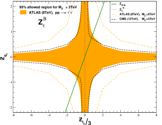
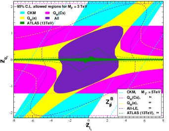
Figure 1: Colored regions correspond to the allowed parameter space at the 95% C.L for a $M_{Z^{\prime}}=3$TeV. The orange region in the left plot in the top panel corresponds to the 95% C.L. allowed by data from proton-proton collisions decaying to tau pairs in the ATLAS detector with an integrated luminosity of $19.5-20.3$ fb^-1. Contours are also shown for the same channel at 13TeV with a luminosity of 2.2 fb^-1 from CMS data. In the remaining plots the green region corresponds to the 95% C.L. allowed region by data proton-proton collisions decaying to electrons and dimuons with an integrated luminosity of 13.3 fb^-1, the magenta region corresponds to the 95% C.L. allowed region by the electron weak charge measurements in Moller scattering. The yellow region corresponds to the 95% C.L. allowed region by the cesium weak charge measurements. The cyan region corresponds to the allowed region by the constraints on the violation of the first-row CKM unitarity [63]. By combining all the data the 95% C.L. allowed parameter space corresponds to the indigo region. The region inside the dashed magenta, yellow, cyan and indigo correspond to the 95% allowed regions for a $M_{Z^{\prime}}=5$TeV. The $Z_{\text{min}}^{\bf B}$ model is basically excluded for a $M_{Z^{\prime}}=$3TeV, for this reason this contour is not shown.

5 Conclusions

In the present work, we presented the most general chiral charges of the minimal universal and non-universal $Z^{\prime}$ model with a minimal content of fermions. Even though, several minimal models have been reported before, the complete solution as a function of a set of continuous parameters and its corresponding collider and low energy constraints, as far as we know, is a new result in the literature.

In general, minimal models are of a great interest for the beyond SM phenomenology [2, 3, 7, 8, 64, 65, 66, 67, 68, 69]. In particle physics the Non-universal models are well motivated, especially in String theory derived constructions, where the $U(1)^{\prime}$ charges are family non-universal [6]. Non-universal models have also been used to explain the number of families and the hierarchies in the fermion spectrum in the SM [15, 16]. In our analysis we rule out some possibilities on phenomenological grounds limiting ourselves to a couple of scenarios to cancel the anomalies. In the simplest case or scenario A the anomalies cancel between fermions in every family. It is fairly obvious that from this scenario, it is possible to obtain, as a particular case, the charges of the minimal universal models which, as it is well known [6], can be written as a linear combination of the charges of the $Z_{B-L}$ model and the SM hypercharge.

In the second case or scenario B the anomalies cancel between fermions in different families. Although it is true that some particular models in this scenario have been reported before, to the best of our knowledge the full parameterization for this scenario is a new result in the literature. To prevent FCNC constraints the charges of the first and second familues were assumed to be identical, but different to the charges of the third family. Constraints from the SM Yukawa interactions were used to impose additional constraints in such a way that the number of free parameters associated with the chiral charges was reduced to four parameters. We also report the most recent LHC constraints on the parameter space for some benchmark models and compare them to those coming from experiments at low energies. From our analysis, we showed that the unitarity constraints on the CKM are able to exclude some regions in the parameter space which are difficult to exclude by using only LHC data.

References

• [1] W. A. Ponce, “Anomaly - Free Version of SU(2) X U(1) X U(1)-prime,” Phys. Rev. D36, 962–965 (1987)
• [2] X. G. He, Girish C. Joshi, H. Lew, and R. R. Volkas, “NEW Z-prime PHENOMENOLOGY,” Phys. Rev. D43, 22–24 (1991)
• [3] Xiao-Gang He, Girish C. Joshi, H. Lew, and R. R. Volkas, “Simplest Z-prime model,” Phys. Rev. D44, 2118–2132 (1991)
• [4] Thomas Appelquist, Bogdan A. Dobrescu, and Adam R. Hopper, “Nonexotic neutral gauge bosons,” Phys. Rev. D68, 035012 (2003), arXiv:hep-ph/0212073 [hep-ph]
• [5] Marcela Carena, Alejandro Daleo, Bogdan A. Dobrescu, and Timothy M. P. Tait, $Z^{\prime}$ gauge bosons at the Tevatron,” Phys. Rev. D70, 093009 (2004), arXiv:hep-ph/0408098 [hep-ph]
• [6] Paul Langacker, “The Physics of Heavy $Z^{\prime}$ Gauge Bosons,” Rev. Mod. Phys. 81, 1199–1228 (2009), arXiv:0801.1345 [hep-ph]
• [7] Ennio Salvioni, Alessandro Strumia, Giovanni Villadoro, and Fabio Zwirner, “Non-universal minimal Z’ models: present bounds and early LHC reach,” JHEP 03, 010 (2010), arXiv:0911.1450 [hep-ph]
• [8] Andreas Crivellin, Giancarlo D’Ambrosio, and Julian Heeck, “Addressing the LHC flavor anomalies with horizontal gauge symmetries,” Phys. Rev. D91, 075006 (2015), arXiv:1503.03477 [hep-ph]
• [9] Ernest Ma, “Progressive Gauge U(1) Family Symmetry for Quarks and Leptons,” Phys. Rev. D94, 031701 (2016), arXiv:1606.06679 [hep-ph]
• [10] Corey Kownacki, Ernest Ma, Nicholas Pollard, and Mohammadreza Zakeri, “Generalized Gauge U(1) Family Symmetry for Quarks and Leptons,” Phys. Lett. B766, 149–152 (2017), arXiv:1611.05017 [hep-ph]
• [11] Randolf Pohl et al.“The size of the proton,” Nature 466, 213–216 (2010)
• [12] R Aaij et al. (LHCb), “Measurement of Form-Factor-Independent Observables in the Decay $B^{0}\to K^{*0}\mu^{+}\mu^{-}$,” Phys. Rev. Lett. 111, 191801 (2013), arXiv:1308.1707 [hep-ex]
• [13] A. J. Krasznahorkay et al.“Observation of Anomalous Internal Pair Creation in Be8 : A Possible Indication of a Light, Neutral Boson,” Phys. Rev. Lett. 116, 042501 (2016), arXiv:1504.01527 [nucl-ex]
• [14] Arno Heister, “Observation of an excess at 30 GeV in the opposite sign di-muon spectra of ${\rm Z}\to b\overline{b}+{\rm X}$ events recorded by the ALEPH experiment at LEP,” (2016), arXiv:1610.06536 [hep-ex]
• [15] F. Pisano and V. Pleitez, “An SU(3) x U(1) model for electroweak interactions,” Phys. Rev. D46, 410–417 (1992), arXiv:hep-ph/9206242 [hep-ph]
• [16] P. H. Frampton, “Chiral dilepton model and the flavor question,” Phys. Rev. Lett. 69, 2889–2891 (1992)
• [17] S. F. Mantilla, R. Martinez, and F. Ochoa, “Neutrino and CP-even Higgs boson masses in a nonuniversal $\mathrm{U}(1)^{\prime}$ extension,” (2016), arXiv:1612.02081 [hep-ph]
• [18] Camilo Salazar, Richard H. Benavides, William A. Ponce, and Eduardo Rojas, “LHC Constraints on 3-3-1 Models,” JHEP 07, 096 (2015), arXiv:1503.03519 [hep-ph]
• [19] Stephen Godfrey and Travis Martin, “Z’ Discovery Reach at Future Hadron Colliders: A Snowmass White Paper,” in Proceedings, Community Summer Study 2013: Snowmass on the Mississippi (CSS2013): Minneapolis, MN, USA, July 29-August 6, 2013 (2013) arXiv:1309.1688 [hep-ph]https://inspirehep.net/record/1253126/files/arXiv:1309.1688.pdf
• [20] Jens Erler, Paul Langacker, Shoaib Munir, and Eduardo Rojas, “Improved Constraints on Z-prime Bosons from Electroweak Precision Data,” JHEP 08, 017 (2009), arXiv:0906.2435 [hep-ph]
• [21] Jens Erler, Paul Langacker, Shoaib Munir, and Eduardo Rojas, “Z’ Bosons at Colliders: a Bayesian Viewpoint,” JHEP 11, 076 (2011), arXiv:1103.2659 [hep-ph]
• [22] Oscar Rodríguez, Richard H. Benavides, William A. Ponce, and Eduardo Rojas, “Flipped versions of the universal 3-3-1 and the left-right symmetric models in $[SU(3)]^{3}$: a comprehensive approach,” Phys. Rev. D95, 014009 (2017), arXiv:1605.00575 [hep-ph]
• [23] K. S. Babu, Borut Bajc, and Vasja Susič, “A minimal supersymmetric E6 unified theory,” JHEP 05, 108 (2015), arXiv:1504.00904 [hep-ph]
• [24] J. C. Montero, F. Pisano, and V. Pleitez, “Neutral currents and GIM mechanism in SU(3)-L x U(1)-N models for electroweak interactions,” Phys. Rev. D47, 2918–2929 (1993), arXiv:hep-ph/9212271 [hep-ph]
• [25] Robert Foot, Oscar F. Hernandez, F. Pisano, and V. Pleitez, “Lepton masses in an SU(3)-L x U(1)-N gauge model,” Phys. Rev. D47, 4158–4161 (1993), arXiv:hep-ph/9207264 [hep-ph]
• [26] Robert Foot, Hoang Ngoc Long, and Tuan A. Tran, $SU(3)_{L}\otimes U(1)_{N}$ and $SU(4)_{L}\otimes U(1)_{N}$ gauge models with right-handed neutrinos,” Phys. Rev. D50, R34–R38 (1994), arXiv:hep-ph/9402243 [hep-ph]
• [27] Murat Ozer, “SU(3)-L x U(1)-x model of the electroweak interactions without exotic quarks,” Phys. Rev. D54, 1143–1149 (1996)
• [28] William A. Ponce, Juan B. Florez, and Luis A. Sanchez, “Analysis of SU(3)(c) x SU(3)(L) x U(1)(X) local gauge theory,” Int. J. Mod. Phys. A17, 643–660 (2002), arXiv:hep-ph/0103100 [hep-ph]
• [29] William A. Ponce, Yithsbey Giraldo, and Luis A. Sanchez, “Minimal scalar sector of 3-3-1 models without exotic electric charges,” Phys. Rev. D67, 075001 (2003), arXiv:hep-ph/0210026 [hep-ph]
• [30] Hiroshi Okada, Nobuchika Okada, and Yuta Orikasa, “Radiative seesaw mechanism in a minimal 3-3-1 model,” Phys. Rev. D93, 073006 (2016), arXiv:1504.01204 [hep-ph]
• [31] Qing-Hong Cao and Dong-Ming Zhang, “Collider Phenomenology of the 3-3-1 Model,” (2016), arXiv:1611.09337 [hep-ph]
• [32] Farinaldo S. Queiroz, Clarissa Siqueira, and José W. F. Valle, “Constraining Flavor Changing Interactions from LHC Run-2 Dilepton Bounds with Vector Mediators,” Phys. Lett. B763, 269–274 (2016), arXiv:1608.07295 [hep-ph]
• [33] Rodolfo A. Diaz, R. Martinez, and F. Ochoa, “SU(3)(c) x SU(3)(L) x U(1)(X) models for beta arbitrary and families with mirror fermions,” Phys. Rev. D72, 035018 (2005), arXiv:hep-ph/0411263 [hep-ph]
• [34] A. E. Carcamo Hernandez, R. Martinez, and F. Ochoa, “Z and Z’ decays with and without FCNC in 331 models,” Phys. Rev. D73, 035007 (2006), arXiv:hep-ph/0510421 [hep-ph]
• [35] R. Aaij et al. (LHCb), “Differential branching fraction and angular analysis of the decay $B^{0}\to K^{*0}\mu^{+}\mu^{-}$,” JHEP 08, 131 (2013), arXiv:1304.6325 [hep-ex]
• [36] Sebastian Jäger and Jorge Martin Camalich, “Reassessing the discovery potential of the $B\to K^{*}\ell^{+}\ell^{-}$ decays in the large-recoil region: SM challenges and BSM opportunities,” Phys. Rev. D93, 014028 (2016), arXiv:1412.3183 [hep-ph]
• [37] Ernest Ma, “Gauged B - 3L(tau) and radiative neutrino masses,” Phys. Lett. B433, 74–81 (1998), arXiv:hep-ph/9709474 [hep-ph]
• [38] Ernest Ma and D. P. Roy, “Phenomenology of the $B$ - 3L($\tau$) gauge boson,” Phys. Rev. D58, 095005 (1998), arXiv:hep-ph/9806210 [hep-ph]
• [39] Ernest Ma and Utpal Sarkar, “Gauged B - 3L(tau) and baryogenesis,” Phys. Lett. B439, 95–102 (1998), arXiv:hep-ph/9807307 [hep-ph]
• [40] Palash B. Pal and Utpal Sarkar, “Gauged B - 3L(tau), low-energy unification and proton decay,” Phys. Lett. B573, 147–152 (2003), arXiv:hep-ph/0306088 [hep-ph]
• [41] Hiroshi Okada, “Dark Matters in Gauged $B-3L_{i}$ Model,” (2012), arXiv:1212.0492 [hep-ph]
• [42] Marco Cirelli, Mario Kadastik, Martti Raidal, and Alessandro Strumia, “Model-independent implications of the e+-, anti-proton cosmic ray spectra on properties of Dark Matter,” Nucl. Phys. B813, 1–21 (2009), [Addendum: Nucl. Phys.B873,530(2013)], arXiv:0809.2409 [hep-ph]
• [43] Patrick J. Fox and Erich Poppitz, “Leptophilic Dark Matter,” Phys. Rev. D79, 083528 (2009), arXiv:0811.0399 [hep-ph]
• [44] Xiao-Jun Bi, Xiao-Gang He, and Qiang Yuan, “Parameters in a class of leptophilic models from PAMELA, ATIC and FERMI,” Phys. Lett. B678, 168–173 (2009), arXiv:0903.0122 [hep-ph]
• [45] Andriy Kurylov and Marc Kamionkowski, “Generalized analysis of weakly interacting massive particle searches,” Phys. Rev. D69, 063503 (2004), arXiv:hep-ph/0307185 [hep-ph]
• [46] F. Giuliani, “Are direct search experiments sensitive to all spin-independent WIMP candidates?.” Phys. Rev. Lett. 95, 101301 (2005), arXiv:hep-ph/0504157 [hep-ph]
• [47] Spencer Chang, Jia Liu, Aaron Pierce, Neal Weiner, and Itay Yavin, “CoGeNT Interpretations,” JCAP 1008, 018 (2010), arXiv:1004.0697 [hep-ph]
• [48] Zhaofeng Kang, Tianjun Li, Tao Liu, Chunli Tong, and Jin Min Yang, “Light Dark Matter from the $U(1)_{X}$ Sector in the NMSSM with Gauge Mediation,” JCAP 1101, 028 (2011), arXiv:1008.5243 [hep-ph]
• [49] Carlos E. Yaguna, “Isospin-violating dark matter in the light of recent data,” Phys. Rev. D95, 055015 (2017), arXiv:1610.08683 [hep-ph]
• [50] Paul Langacker and Ming-xing Luo, “Constraints on additional $Z$ bosons,” Phys. Rev. D45, 278–292 (1992)
• [51] Jens Erler, Paul Langacker, Shoaib Munir, and Eduardo Rojas, $Z^{\prime}$ Bosons from E(6): Collider and Electroweak Constraints,” in 19th International Workshop on Deep-Inelastic Scattering and Related Subjects (DIS 2011) Newport News, Virginia, April 11-15, 2011 (2011) arXiv:1108.0685 [hep-ph]https://inspirehep.net/record/921984/files/arXiv:1108.0685.pdf
• [52] Eduardo Rojas and Jens Erler, “Alternative Z bosons in E6,” JHEP 10, 063 (2015), arXiv:1505.03208 [hep-ph]
• [53] Jonathan L. Feng, Bartosz Fornal, Iftah Galon, Susan Gardner, Jordan Smolinsky, Tim M. P. Tait, and Philip Tanedo, “Protophobic Fifth-Force Interpretation of the Observed Anomaly in 8Be Nuclear Transitions,” Phys. Rev. Lett. 117, 071803 (2016), arXiv:1604.07411 [hep-ph]
• [54] The ATLAS collaboration (ATLAS), “Search for new high-mass resonances in the dilepton final state using proton-proton collisions at $\sqrt{s}$ = 13 TeV with the ATLAS detector,” (2016)
• [55] Georges Aad et al. (ATLAS), “A search for high-mass resonances decaying to $\tau^{+}\tau^{-}$ in $pp$ collisions at $\sqrt{s}=8$ TeV with the ATLAS detector,” JHEP 07, 157 (2015), arXiv:1502.07177 [hep-ex]
• [56] CMS Collaboration (CMS), “Search for new physics with high-mass tau lepton pairs in pp collisions at sqrt(s) = 13 TeV with the CMS detector,” (2016)
• [57] Carlos Felipe Gonzalez Hernandez (CMS), “Search for new physics with high-mass $\tau$-lepton pairs in pp collisions at 13 TeV with the CMS detector,” Proceedings, 4th Large Hadron Collider Physics Conference (LHCP 2016): Lund, Sweden, June 13-18, 2016, PoS LHCP2016, 220 (2016)
• [58] C. S. Wood, S. C. Bennett, D. Cho, B. P. Masterson, J. L. Roberts, C. E. Tanner, and Carl E. Wieman, “Measurement of parity nonconservation and an anapole moment in cesium,” Science 275, 1759–1763 (1997)
• [59] J. Guena, M. Lintz, and M. A. Bouchiat, “Measurement of the parity violating 6S-7S transition amplitude in cesium achieved within 2 x 10(-13) atomic-unit accuracy by stimulated-emission detection,” Phys. Rev. A71, 042108 (2005), arXiv:physics/0412017 [physics.atom-ph]
• [60] P. L. Anthony et al. (SLAC E158), “Precision measurement of the weak mixing angle in Moller scattering,” Phys. Rev. Lett. 95, 081601 (2005), arXiv:hep-ex/0504049 [hep-ex]
• [61] W. J. Marciano and A. Sirlin, “Constraint on Additional Neutral Gauge Bosons From Electroweak Radiative Corrections,” Phys. Rev. D35, 1672–1676 (1987)
• [62] Andrzej J. Buras, Fulvia De Fazio, and Jennifer Girrbach, “331 models facing new $b\to s\mu^{+}\mu^{-}$ data,” JHEP 02, 112 (2014), arXiv:1311.6729 [hep-ph]
• [63] K. A. Olive et al. (Particle Data Group), “Review of Particle Physics,” Chin. Phys. C38, 090001 (2014)
• [64] Alejandro Celis, Javier Fuentes-Martin, Martín Jung, and Hugo Serodio, “Family nonuniversal Z models with protected flavor-changing interactions,” Phys. Rev. D92, 015007 (2015), arXiv:1505.03079 [hep-ph]
• [65] F. M. L. Almeida, Jr., Yara do Amaral Coutinho, Jose Antonio Martins Simoes, J. Ponciano, A. J. Ramalho, Stenio Wulck, and M. A. B. Vale, “Minimal left-right symmetric models and new Z’ properties at future electron-positron colliders,” Eur. Phys. J. C38, 115–122 (2004), arXiv:hep-ph/0405020 [hep-ph]
• [66] Durmus A. Demir, Gordon L. Kane, and Ting T. Wang, “The Minimal U(1)’ extension of the MSSM,” Phys. Rev. D72, 015012 (2005), arXiv:hep-ph/0503290 [hep-ph]
• [67] Elena Accomando, Claudio Coriano, Luigi Delle Rose, Juri Fiaschi, Carlo Marzo, and Stefano Moretti, “Z, Higgses and heavy neutrinos in U(1) models: from the LHC to the GUT scale,” JHEP 07, 086 (2016), arXiv:1605.02910 [hep-ph]
• [68] Elena Accomando, Claudio Coriano, Luigi Delle Rose, Juri Fiaschi, Carlo Marzo, and Stefano Moretti, “Phenomenology of minimal Z’ models: from the LHC to the GUT scale,” Proceedings, 8th International Workshop on Quantum Chromodynamics - Theory and Experiment (QCD@Work 2016): Martina Franca, Italy, June 27-30, 2016EPJ Web Conf. 129, 00006 (2016), arXiv:1609.05029 [hep-ph]
• [69] Lorenzo Basso, “Minimal Z’ models and the 125 GeV Higgs boson,” Phys. Lett. B725, 322–326 (2013), arXiv:1303.1084 [hep-ph]